Triangular and $Y$-shaped hadrons with static sources

Abstract

The structure of hadrons consisting of three static color sources in fundamental (baryons) or adjoint (three-gluon glueballs) representations is studied. The static potentials of glueballs as well as gluon field distributions in glueballs and baryons are calculated in the framework of field correlator method.

1. The study of the gluon field structure in hadrons is important for the deep understanding of the strong interaction physics. Interesting results on the baryon flux structure were obtained recently in the maximally abelian gauge on the lattice [1]. We demonstrate below how to perform calculations in gauge invariant way using the field correlator method relyed directly on QCD.

The static potential in baryon was considered in detail in [2] at this conference, and we will extensively refer to this talk in what follows. We start with the calculations of static potentials in three-gluon glueballs. This part of the talk presents the results from [3]. In the rest of the talk the gluon field distributions in hadrons are discussed on the base of papers [4], [5], [6].

In contrast to baryons, the gauge-invariant extended wave function of glueballs may have both $Y$-type and triangular structure. In the former case it may be written as

$$G^{(f)}_{Y}(x,y,z,Y)=f^{abc}g_{a}(x,Y)g_{b}(y,Y)g_{c}(z,Y)\quad\mbox{ or}$$ (1)

$$G^{(g)}_{Y}(x,y,z,Y)=g^{abc}g_{a}(x,Y)g_{b}(y,Y)g_{c}(z,Y).$$ (2)

Here $g_{a}(x,Y)=g_{a}(x)\Phi^{ab}(x,Y)$ denotes the extended gluon operator, $g_{a}(x)$ is the valence gluon operator and $\Phi^{ab}(x,Y)=(\mathrm{P}\exp ig\int_{Y}^{x}A_{\mu}dz_{\mu})^{ab}$ is the parallel transporter or Schwinger line in the adjoint representation. The coordinates $x,y,z$ and $Y$ in (1) apply to the valence gluons and string junction positions respectively, $f^{abc}$ and $g^{abc}$ denote adjoint antisymmetric and symmetric symbols.

The wave function of the triangular glueball has the form

$$G_{\Delta}(x,y,z)=G_{\alpha}^{\beta}(x)\Phi_{\beta}^{\gamma}(x,y)G_{\gamma}^{\delta}(y)\Phi_{\delta}^{\varepsilon}(y,z)G_{\varepsilon}^{\rho}(z)\Phi_{\rho}^{\alpha}(z,x),$$ (3)

where $G_{\alpha}^{\beta}(x)=g^{a}(x)(t^{a})_{\alpha}^{\beta}$, $t$ is the generator of $SU(3)$, and $\Phi_{\alpha}^{\beta}$ is the parallel transporter in fundamental representation.

According to (1), (2), a Wilson loop of $Y$-type glueball has the same structure as in the case of baryon, see eq. (2) and Fig. 1 of [2]. The difference is that the adjoint transporters should be substituted for the fundamental ones and symbols $f^{abc}$ or $g^{abc}$ for $\epsilon_{\alpha\beta\gamma}$.

A Wilson loop of triangular glueball, induced by (3) in the limit of large $N_{c}$, is shown in Fig. 1. The trajectories of valence gluons are replaced here with two fundamental (quark) trajectories and the Wilson loop is reduced to three disconnected rectangular meson loops.

The static potential in baryon calculated in the field correlator method (MFC) is proportional to two-point gluon field strength correlators in fundamental representation, see e.g. (5), (6) from [2]. Therefore it is proportional to the fundamental Casimir operator, $C_{F}=4/3$, and the ratio of $Y$-type glueball and baryon potentials equals to the ratio of corresponding Casimir operators,

Figure 1: $\Delta$-type Wilson loop

$$\frac{V_{Y}^{(G)}}{V_{Y}^{(B)}}=\frac{C_{A}}{C_{F}}=\frac{9}{4},$$ (4)

where $C_{A}=3$ is the adjoint Casimir operator and nondiagonal (interference) terms are neglected. The diagonal part of the baryon potential in equilateral triangle has the form [3]

$$V_{Y}^{(B)}(R)=\frac{6\sigma}{\pi}\left\{R\int_{0}^{R/T_{g}}dx\,xK_{1}(x)-T_{g}\left(2-\frac{R^{2}}{T_{g}^{2}}K_{2}\left(\frac{R}{T_{g}}\right)\right)\right\}\equiv 3V^{(M)}(R),$$ (5)

where $R$ is the distance from quarks to string junction, $K_{1},~{}K_{2}$ are McDonald functions, $\sigma$=0.18 GeV² and $T_{g}=0.12\div 0.2$ fm are the string tension and the gluon field correlation length, and $V^{(M)}(R)$ is the static potential in meson.

Figure 2: Glueball potentials $V_{Y}^{(G)}(r)+V^{\mathrm{pert}}_{\mathrm{(adj)}}(r)$ (solid curve) and $V_{\Delta}^{(G)}(r)+V^{\mathrm{pert}}_{\mathrm{(adj)}}(r)$ (dashed curve) in equilateral triangle with the quark separations $r$ for $\alpha_{s}=0.3$, $\sigma$=0.18 GeV² and $T_{g}=0.12$ fm. The nondiagonal terms are neglected.

Now we turn to the triangular glueball, whose Wilson loop according to Fig. 1 is the product of three meson loops. Therefore, the potential $V_{\Delta}^{(G)}$, which is the logarithm of the Wilson loop, is the sum of three meson potentials. In the case of equilateral triangle with the side $r=\sqrt{3}R$

$$V_{\Delta}^{(G)}(r)=3V^{(M)}(r).$$ (6)

The perturbative potential for three-gluon glueballs reads as

$$V^{\mathrm{pert}}_{\mathrm{(adj)}}(r)=-\frac{3}{2}\,\frac{C_{2}(\mathrm{adj})\alpha_{s}}{r}.$$ (7)

The behavior of total potentials in $Y$-type and triangular glueballs are shown in Fig. 2. One can see that they are very close up to distances $r\approx 0.6$ fm. Note that the interference terms are to change this picture. They will be considered in subsequent publications.

2. We proceed now to the study of the gluon field structure using the connected probe [7], [8]. The connected probe consists of the probe plaquette joined to the Wilson loop by parallel transporters and forms the frame with the current in four-dimentional euclidian space, see Fig. 3. When the plaquette size is small enough, the connected probe affords to calculate the color-integrated gluon field in hadron, using the Wilson loop $\cal W^{H}$ of the latter,

$$F^{H}_{\mu\nu}(x)=-ig\,\frac{\langle{\cal W^{H}}^{\alpha}_{\beta}(x_{0})\Phi^{\beta}_{\gamma}(x_{0},x)(F_{\mu\nu}^{a}(x)t^{a})^{\gamma}_{\delta}(\Phi^{+})^{\delta}_{\alpha}(x,x_{0})\rangle}{\langle{\cal W^{H}}\rangle}.$$ (8)

The following expression is valid in the bilocal approximation of MFC in the case of mesons [5],

$$F^{M}_{\mu\nu}(x)=\int_{S}d\sigma_{\rho\sigma}(x^{\prime})\,{\cal D}_{\rho\sigma,\mu\nu}(x^{\prime}-x),$$ (9)

where the integration is taken over the surface of Wilson loop $S$ and ${\cal D}$ denotes the gauge-invariant bilocal gluon field strenth correlator, see e.g. (5) of [2] for details. Using the MFC parametrization of correlators [2], we calculate that the electric component of the $F^{M}$ has the form [6]

$$\mbox{\boldmath${\rm E}$}^{M}(\mbox{\boldmath${\rm x}$},\mbox{\boldmath${\rm R}$})=\mbox{\boldmath${\rm n}$}\,\frac{2\sigma}{\pi}\int_{0}^{R/T_{g}}dl\,\left|l\mbox{\boldmath${\rm n}$}-\frac{\mbox{\boldmath${\rm x}$}}{T_{g}}\right|K_{1}\left(\left|l\mbox{\boldmath${\rm n}$}-\frac{\mbox{\boldmath${\rm x}$}}{T_{g}}\right|\right),$$ (10)

while the magnetic one is absent.

The field $\mbox{\boldmath${\rm E}$}^{M}(\mbox{\boldmath${\rm x}$},\mbox{\boldmath${\rm R}$})$ (10), which we call the nonperturbative background gluon field in meson, is the force acting on the probe located at the point ${\rm x}$ while the quark situated at zero and antiquark at the point ${\rm R}$. It is related to the field acting on the quark as follows.

The force $\mbox{\boldmath${\rm F}$}^{M}$ acting on the quark in meson is defined by the static potential $V^{(M)}$ (5),

$$\mbox{\boldmath${\rm F}$}^{M}(\mbox{\boldmath${\rm r}$})=-\mbox{\boldmath${\rm\nabla}$}V^{(M)}(\mbox{\boldmath${\rm r}$}).$$ (11)

Figure 3: A connected probe in the case of meson

One can verify using (5), (10), (11) that the following relations are valid [6],

$$\mbox{\boldmath${\rm E}$}^{M}(0,\mbox{\boldmath${\rm R}$})=\mbox{\boldmath${\rm E}$}^{M}(\mbox{\boldmath${\rm R}$},\mbox{\boldmath${\rm R}$})=\mbox{\boldmath${\rm F}$}^{M}(\mbox{\boldmath${\rm R}$}),$$ (12)

$$\mbox{\boldmath${\rm E}$}^{M}(\mbox{\boldmath${\rm R}$},2\mbox{\boldmath${\rm R}$})=\mbox{\boldmath${\rm E}$}^{M}(0,\mbox{\boldmath${\rm R}$})+\mbox{\boldmath${\rm E}$}^{M}(\mbox{\boldmath${\rm R}$},\mbox{\boldmath${\rm R}$})=2\mbox{\boldmath${\rm F}$}^{M}(\mbox{\boldmath${\rm R}$}).$$ (13)

The relation (12) mean that when the locations of probe and quark (antiquark) coinside, the probe recombines with the latter, and that is why it is affected by the same force $\mbox{\boldmath${\rm F}$}^{M}$. One can conclude from the relation (13) that when the probe is situated in the middle of two sources, it interacts with both the quark and antiquark, and the total field becomes twice as big. If the point ${\rm x}$ is located on the line connecting the quark and antiquark, it is easy to check using (5), (10) that the generalization of (12), (13) has the form

$$\mbox{\boldmath${\rm E}$}^{M}(\mbox{\boldmath${\rm x}$},\mbox{\boldmath${\rm R}$})=\mbox{\boldmath${\rm F}$}^{M}(\mbox{\boldmath${\rm x}$})-\mbox{\boldmath${\rm F}$}^{M}(\mbox{\boldmath${\rm x}$}-\mbox{\boldmath${\rm R}$}).$$ (14)

According to (11), the force $\mbox{\boldmath${\rm F}$}^{M}(\mbox{\boldmath${\rm R}$})$ acting on the quark increases linearly with the slope $2\sigma/(\pi T_{g})$ at small distances $R\mathrel{\mathchoice{\lower 3.6pt\vbox{\halign{$\mathsurround=0pt\displaystyle\hfil#\hfil$\cr<\crcr\sim\crcr}}}{\lower 3.6pt\vbox{\halign{$\mathsurround=0pt\textstyle\hfil#\hfil$\cr<\crcr\sim\crcr}}}{\lower 3.6pt\vbox{\halign{$\mathsurround=0pt\scriptstyle\hfil#\hfil$\cr<\crcr\sim\crcr}}}{\lower 3.6pt\vbox{\halign{$\mathsurround=0pt\scriptscriptstyle\hfil#\hfil$\cr<\crcr\sim\crcr}}}}T_{g}$ and saturates with the value $\sigma$ at $R\mathrel{\mathchoice{\lower 3.6pt\vbox{\halign{$\mathsurround=0pt\displaystyle\hfil#\hfil$\cr>\crcr\sim\crcr}}}{\lower 3.6pt\vbox{\halign{$\mathsurround=0pt\textstyle\hfil#\hfil$\cr>\crcr\sim\crcr}}}{\lower 3.6pt\vbox{\halign{$\mathsurround=0pt\scriptstyle\hfil#\hfil$\cr>\crcr\sim\crcr}}}{\lower 3.6pt\vbox{\halign{$\mathsurround=0pt\scriptscriptstyle\hfil#\hfil$\cr>\crcr\sim\crcr}}}}0.7$ fm.

The field $\mbox{\boldmath${\rm E}$}^{M}$ in the saturated regime acquires the universal profile $E^{\mathrm{string}}$, which does not depend on the quark-antiquark separation,

$$E^{\mathrm{string}}(\rho)=2\sigma\left(1+\frac{\rho}{T_{g}}\right)\exp\left(-\frac{\rho}{T_{g}}\right),$$ (15)

where $\rho$ is the distance from the quark-antiquark axis. We apply now the Gauss law in the form

$$\int\mbox{\boldmath${\rm E}$}\,d\mbox{\boldmath${\rm S}$}=4\pi C_{F}\alpha_{s}$$ (16)

to the saturated field (15) and get the parameter relation

$$3\,\sigma T_{g}=C_{F}\alpha_{s}.$$ (17)

Taking the freezing value of the strong coupling $\alpha_{s}\approx 0.4$ [9] and the phenomenological value of the string tension $\sigma=0.18$ GeV², we determine from (17) the reasonable gluon correlation length value $T_{g}\approx 0.2$ fm (see [2]).

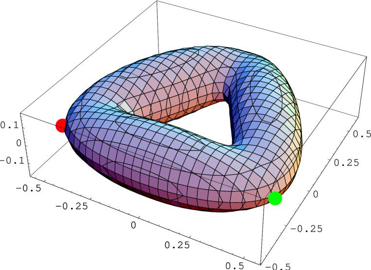
Figure 4: The contour plot of the field in the $\Delta$-type three-gluon glueball. The valence gluon separations are 1 fm, $\sigma=0.18$ GeV², $T_{g}=0.12$ fm.

Using the Maxwell equation with magnetic currents,

$$\mathrm{rot}\,\mbox{\boldmath${\rm E}$}^{M}=\mbox{\boldmath${\rm j}$}_{\mathrm{magn}},$$ (18)

we obtain that currents corresponding to the saturated field (15) form closed circles around the quark-antiquark axis, with the density

$$j_{\mathrm{magn}}(\rho)=\frac{\partial E^{\mathrm{string}}(\rho)}{\partial\rho}=\frac{2\sigma\rho}{T_{g}^{2}}\exp\left(-\frac{\rho}{T_{g}}\right).$$ (19)

One can verify using (9), (18) and nonabelian Bianchi identity that magnetic currents arise due to the three-point field strength correlator, which describes the emitting of the color-magnetic gluon field by the color-electric one.

The detailed study of these and other properties of the field $\mbox{\boldmath${\rm E}$}^{M}$ will be given elsewhere.

3. When the field distribution of the quark-antiquark pair is known, it is straightforward to calculate the field of triangular glueball (see Fig. 1). We join the connected probe to each of quark-antiquark loops and arrive at the expression

$$\mbox{\boldmath${\rm E}$}_{\Delta}^{(G)}(\mbox{\boldmath${\rm x}$},\mbox{\boldmath${\rm r}$}^{(1)},\mbox{\boldmath${\rm r}$}^{(2)},\mbox{\boldmath${\rm r}$}^{(3)})=\sum_{i=1}^{3}\mbox{\boldmath${\rm E}$}^{M}(\mbox{\boldmath${\rm x}$}-\mbox{\boldmath${\rm r}$}^{(i)},\mbox{\boldmath${\rm R}$}^{(i)}),$$ (20)

where $\mbox{\boldmath${\rm r}$}^{(i)}$ is the position of $i$-th valence gluon and $\mbox{\boldmath${\rm R}$}^{(i)}=\mbox{\boldmath${\rm r}$}^{(i+1)}-\mbox{\boldmath${\rm r}$}^{(i)}$. The surface defined by the condition $|\mbox{\boldmath${\rm E}$}_{\Delta}^{(G)}(\mbox{\boldmath${\rm x}$})|=\sigma$ at gluon separations 1 fm is shown in Fig. 4. Values of parameters $\sigma=0.18$ GeV², $T_{g}=0.12$ fm are used. The surface shown in the figure goes through the valence gluon locations. Indeed, one can verify using (20) that two forces of the value $\sigma$ having the angle $2\pi/3$ between them add to give the resulting force of the value $\sigma$.

The same procedure can be applied to the system of arbitrary number of mesons to obtain the field distributions in the leading order of $1/N_{c}$. The next order corrections can also be considered within the approach.

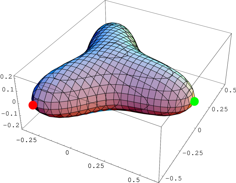
Figure 5: The contour plot of the field in the baryon. The quark separations are 1 fm, $\sigma=0.18$ GeV², $T_{g}=0.12$ fm.

4. The problem of baryon (or $Y$-type glueball) field calculations is more complicated. When we join the probe plaquette to the trajectory of the first quark and calculate the field distribution (8) using the bilocal approximation of MFC, we arrive at the following relation for the electric field,

$$\mbox{\boldmath${\rm E}$}^{B}_{(1)}(\mbox{\boldmath${\rm x}$},\mbox{\boldmath${\rm R}$}^{(1)},\mbox{\boldmath${\rm R}$}^{(2)},\mbox{\boldmath${\rm R}$}^{(3)})=\mbox{\boldmath${\rm E}$}^{M}(\mbox{\boldmath${\rm x}$},\mbox{\boldmath${\rm R}$}^{(1)})-\frac{1}{2}\,\mbox{\boldmath${\rm E}$}^{M}(\mbox{\boldmath${\rm x}$},\mbox{\boldmath${\rm R}$}^{(2)})-\frac{1}{2}\,\mbox{\boldmath${\rm E}$}^{M}(\mbox{\boldmath${\rm x}$},\mbox{\boldmath${\rm R}$}^{(3)})$$ (21)

(the magnetic field is absent just as in the meson case). The vector $\mbox{\boldmath${\rm R}$}^{(i)}$ here is directed from the string junction to the $i$-th quark, $\mbox{\boldmath${\rm E}$}^{M}$ is defined in (10). When we join the probe to the second and third quark trajectories, we will get analogous formulas with the corresponding index transpositions.

To obtain symmetric field distributions, we are to sum squares $(\mbox{\boldmath${\rm E}$}^{B}_{(i)})^{2}$,

$$(\mbox{\boldmath${\rm E}$}^{(B)})^{2}=\frac{2}{3}\,\left((\mbox{\boldmath${\rm E}$}^{B}_{(1)})^{2}+(\mbox{\boldmath${\rm E}$}^{B}_{(2)})^{2}+(\mbox{\boldmath${\rm E}$}^{B}_{(3)})^{2}\right),$$ (22)

The surface given by the condition $|\mbox{\boldmath${\rm E}$}^{(B)}(\mbox{\boldmath${\rm x}$})|=\sigma$ at quark separations 1 fm is shown in Fig. 4. It goes through the quark positions and has small convexity near the string junction.

The ratio of the energy density at the string junction position, $w_{\mathrm{sj}}$, to the density in the middle of the string with the saturated profile, $w_{\mathrm{string}}$, has to be equal to the corresponding field squares and according to (22), (15)

$$\frac{w_{\mathrm{sj}}}{w_{\mathrm{string}}}=\frac{(\mbox{\boldmath${\rm E}$}^{(B)}(0))^{2}}{(\mbox{\boldmath${\rm E}$}^{\mathrm{string}}(0))^{2}}=\frac{9}{8}.$$ (23)

To conclude, hadron static potentials and the gluon field distributions, which ensure the confinement of color sources, were calculated using the field correlator method. It is stressed that the mechanism of confinement is the emitting process of the color-magnetic gluon field by the color-electric one in the nonperturbative vacuum. The static potentials of three-gluon glueballs were reduced in the first approximation to the appropriate sum of quark-antiquark potentials. The nonperturbative gluon field induced by the static quark-antiquark pair was calculated using the connected probe, and its classical abelian properties were considered. Triangular gluon field distributions were calculated for glueballs and $Y$-type ones for baryons.

An extension of the method to the arbitrary number of colors is straightforward. It is also applicable to the nuclear structure study.

This work has been supported by RFBR grants 00-02-17836, 00-15-96786, and INTAS 00-00110, 00-00366.

References

• [1] H. Ichie, V. Bornyakov, T. Streuer, G. Schierholz, ITEP-LAT-2002-24, KANAZAWA-02-33, hep-lat/0212024.
• [2] D.S. Kuzmenko, this volume, hep-ph/0302067.
• [3] D.S. Kuzmenko and Yu.A.Simonov, Yad.Fiz. (in press), hep-ph/0202277.
• [4] D.S. Kuzmenko and Yu.A. Simonov, Phys.Lett. B494, 81 (2000).
• [5] D.S. Kuzmenko and Yu.A. Simonov, Yad.Fiz. 64, 110 (2001), hep-ph/0010114.
• [6] D.S. Kuzmenko, ITEP-2002-06 (in russian); Ph.D. thesis, Moscow (2002) (in russian).
• [7] A.Di Giacomo, M.Maggiore and S.Olejnik, Phys.Lett. B236 (1990) 199; Nucl.Phys. B347 (1990) 441
• [8] L.Del Debbio, A.Di Giacomo and Yu.A.Simonov, Phys.Lett. B332 (1994) 111
• [9] A.M. Badalian and D.S. Kuzmenko, Phys.Rev. D65, 016004 (2002).