Two-loop HTL Thermodynamics with Quarks

Abstract

We calculate the quark contribution to the free energy of a hot quark-gluon plasma to two-loop order using hard-thermal-loop (HTL) perturbation theory. All ultraviolet divergences can be absorbed into renormalizations of the vacuum energy and the HTL quark and gluon mass parameters. The quark and gluon HTL mass parameters are determined self-consistently by a variational prescription. Combining the quark contribution with the two-loop HTL perturbation theory free energy for pure-glue we obtain the total two-loop QCD free energy. Comparisons are made with lattice estimates of the free energy for $N_{f}=2$ and with exact numerical results obtained in the large-$N_{f}$ limit.

I Introduction

The current generation of relativistic heavy-ion collision experiments should exceed the energy density necessary for the formation of a quark-gluon plasma. It is therefore necessary to have a quantitative theoretical framework which can be used to calculate the properties of a quark-gluon plasma. The usual line of reasoning is that since QCD is asymptotically free, its running coupling constant $\alpha_{s}$ becomes weaker as the temperature increases and therefore the behavior of hadronic matter at sufficiently high temperature should be calculable using perturbative methods. Unfortunately, a straightforward perturbative expansion in powers of $\alpha_{s}$ does not seem to be of any quantitative use even at temperatures many orders of magnitude higher than those achievable in heavy-ion collisions.

The problem can be seen by looking at the perturbative expansion of the free energy ${\cal F}$ of a quark-gluon plasma, whose weak-coupling expansion has been calculated completely through order $\alpha_{s}^{5/2}$ AZ-95 ; KZ-96 ; BN-96

$${\cal F} = -{8\pi^{2}\over 45}T^{4}\,\left[{\cal F}_{0}\,+\,{\cal F}_{2}{\alpha_{s}\over\pi}\,+\,{\cal F}_{3}\left({\alpha_{s}\over\pi}\right)^{3/2}\right.$$ (1)

$$\left.\,+\,{\cal F}_{4}\left({\alpha_{s}\over\pi}\right)^{2}\,+\,{\cal F}_{5}\left({\alpha_{s}\over\pi}\right)^{5/2}\,+\,O(\alpha_{s}^{3}\log\alpha_{s})\right]\,,$$

with

$${\cal F}_{0} = 1+\textstyle{21\over 32}N_{f}\,,$$ (2)

$${\cal F}_{2} = -{15\over 4}\left(1+\textstyle{5\over 12}N_{f}\right)\;,$$ (3)

$${\cal F}_{3} = 30\left(1+\textstyle{1\over 6}N_{f}\right)^{3/2}\,,$$ (4)

$${\cal F}_{4} = 237.2+15.97N_{f}-0.413N_{f}^{2}$$ (5)

$$\hskip 5.69054pt+{135\over 2}\left(1+\textstyle{1\over 6}N_{f}\right)\log\left[{\alpha_{s}\over\pi}\left(1+\textstyle{1\over 6}N_{f}\right)\right]$$

$$\hskip 5.69054pt-{165\over 8}\left(1+{5\over 12}N_{f}\right)\left(1-{2\over 33}N_{f}\right)\log{\mu\over 2\pi T}\;,$$

$${\cal F}_{5} = -\left(1+\textstyle{1\over 6}N_{f}\right)^{1/2}\Bigg{[}799.2+21.96N_{f}+1.926N_{f}^{2}\Bigg{]}$$ (6)

$$\hskip 5.69054pt+{495\over 2}\left(1+{1\over 6}N_{f}\right)\left(1-{2\over 33}N_{f}\right)\log{\mu\over 2\pi T}\;,$$

where $\mu$ is the renormalization scale, $\alpha_{s}=\alpha_{s}(\mu)$ is the running coupling constant in the $\overline{\mbox{MS}}$ scheme, and we have set $N_{c}=3$. The coefficient of $\alpha_{s}^{3}\log\alpha_{s}$ has recently been computed KLRS-02 ; however, since there are unknown perturbative and non-perturbative contributions at $O(\alpha_{s}^{3})$ we do not include terms higher than $O(\alpha_{s}^{5/2})$ in Eq. (1).

In Fig. 1, the free energy with $N_{f}=2$ is shown as a function of the temperature $T/T_{c}$, where $T_{c}$ is the critical temperature for the deconfinement transition. In the plot we have scaled the free energy by the free energy of an ideal gas of quarks and gluons which for arbitrary $N_{c}$ and $N_{f}$ is

$${\cal F}_{\rm ideal}=-{\pi^{2}\over 45}T^{4}\left(N_{c}^{2}-1+{7\over 4}N_{c}N_{f}\right)\,.$$ (7)

The weak-coupling expansions through orders $\alpha_{s}$, $\alpha_{s}^{3/2}$, $\alpha_{s}^{2}$, and $\alpha_{s}^{5/2}$ are shown as bands that correspond to varying the renormalization scale, $\mu$, by a factor of two around the central value $\mu=2\pi T$. As successive terms in the weak-coupling expansion are added, the predictions change wildly and the sensitivity to the renormalization scale grows. It is clear that a reorganization of the perturbation series is essential if perturbative calculations are to be of any quantitative use at temperatures accessible in heavy-ion collisions.

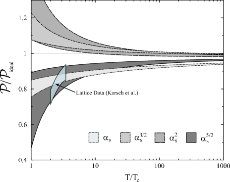
Figure 1: The perturbative free energy of QCD for $N_{f}=2$ massless quarks as a function of $T/T_{c}$. The weak-coupling expansions through orders $\alpha_{s}$, $\alpha_{s}^{3/2}$, $\alpha_{s}^{2}$, and $\alpha_{s}^{5/2}$ are shown as bands that correspond to varying the renormalization scale $\mu$ by a factor of two around $2\pi T$. Also shown is a lattice estimate by Karsch et al. klp for the free energy. The band indicates the estimated systematic error of their result which is reported as (15$\pm$5)%.

The free energy can also be calculated nonperturbatively using lattice gauge theory Karsch . The thermodynamic functions for pure-glue QCD have been calculated with high precision by Boyd et al. lattice-0 . There have also been calculations which include dynamical quarks klp ; lattice-Nf . In Fig. 1 we have included the latest lattice estimate of Karsch et al. klp for the free energy for $N_{f}=2$ flavors of light quarks. The band indicates the estimated systematic error of their result which is reported as (15$\pm$5)%. Note that the quarks in the simulations do have non-zero masses and that extrapolation to zero quark mass would require significant computing time. Due to the difficulty associated with the inclusion of light/massless dynamical quarks on the lattice it is therefore desirable to have analytic methods which can be used to estimate the thermodynamic functions.

The only rigorous method available for reorganizing perturbation theory in thermal QCD is dimensional reduction to an effective 3-dimensional field theory KLRS ; Kajantie-97 . The coefficients of the terms in the effective lagrangian are calculated using perturbation theory, but calculations within the effective field theory are carried out nonperturbatively using lattice gauge theory. Dimensional reduction has the same limitations as ordinary lattice gauge theory: it can be applied only to static quantities and only at zero baryon number density. Unlike in ordinary lattice gauge theory, light dynamical quarks do not require any additional computer power, because they only enter through the perturbatively calculated coefficients in the effective lagrangian. This method has been applied to the Debye screening mass for QCD Kajantie-97 as well as the pressure KLRS .

There are some proposals for reorganizing perturbation theory in QCD that are essentially just mathematical manipulations of the weak coupling expansion. The methods include Padé approximates Pade , Borel resummation Parwani , and self-similar approximates Yukalov . These methods are used to construct more stable sequences of successive approximations that agree with the weak-coupling expansion when expanded in powers of $\alpha_{s}$. These methods can only be applied to quantities for which several orders in the weak-coupling expansion are known, so they are limited in practice to the thermodynamic functions.

One promising approach for reorganizing perturbation theory in thermal QCD is to use a variational framework. The free energy ${\cal F}$ is expressed as the variational minimum of a thermodynamic potential $\Omega(T,\alpha_{s};m^{2})$ that depends on one or more variational parameters that we denote collectively by $m^{2}$:

$${\cal F}(T,\alpha_{s})\;=\;\Omega(T,\alpha_{s};m^{2})\bigg{|}_{\partial\Omega/\partial m^{2}=0}\,.$$ (8)

A particularly compelling variational formulation is the $\Phi$-derivable approximation, in which the complete propagator is used as an infinite set of variational parameters Phi . The $\Phi$-derivable thermodynamic potential $\Omega$ is the 2PI effective action, the sum of all diagrams that are 2-particle-irreducible with respect to the complete propagator CJT-74 . The $n$-loop $\Phi$-derivable approximations, in which $\Omega$ is the the sum of 2PI diagrams with up to $n$ loops, form a systematically improvable sequence of variational approximations. Until recently, $\Phi$-derivable approximations have proved to be intractable for relativistic field theories except for simple cases in which the self-energy is momentum-independent. However there has been some recent progress in solving the 3-loop $\Phi$-derivable approximation for scalar field theories. Braaten and Petitgirard have developed an analytic method for solving the 3-loop $\Phi$-derivable approximation for the massless $\phi^{4}$ field theory BP-01 . Van Hees and Knoll have developed numerical methods for solving the 3-loop $\Phi$-derivable approximation for the massive $\phi^{4}$ field theory vHK-01 . They also investigated renormalization issues associated with the $\Phi$-derivable approximation. These issues have recently been studied in detail by Blaizot, Iancu, and Reinosa BIR-03 .

The application of the $\Phi$-derivable approximation to QCD was first discussed by McLerran and Freedman FM-77 . One problem with this approach is that the thermodynamic potential $\Omega$ is gauge dependent, and so are the resulting thermodynamic functions. The gauge dependence is the same order in $\alpha_{s}$ as the truncation error when evaluated off the stationary point and twice the order in $\alpha_{s}$ when evaluated at the stationary point AS-02 . However the most serious problem is that even the application of 2-loop $\Phi$-derivable approximation to gauge theories has proved to be intractable.

The 2-loop $\Phi$-derivable approximation for QCD has been used as the starting point for HTL resummations of the entropy by Blaizot, Iancu and Rebhan BIR-99 and of the pressure by Peshier Peshier-00 . The thermodynamic potential $\Omega_{\rm 2-loop}$ is a functional of the complete gluon propagator $D_{\mu\nu}(P)$. However, in order to make the problem tractable the authors in Refs. BIR-99 and Peshier-00 were forced to make a variational ansatz for the exact gluon propagator which they took as the HTL gluon propagator in the infrared and free in the ultraviolet with an aribitrary momentum scale separating the two momentum regions. Using this ansatz they were able to calculate the QCD thermodynamic functions; however, a first-principles calculation of the corrections to their results for gauge theories would require the inclusion of exact vertices as well as exact propagators thus making the problem intractable.

The difficulties in calculating quantities using $\Phi$-derivable approximations in gauge theories motivates the use of simpler variational approximations. One such strategy that involves a single variational parameter $m$ has been called optimized perturbation theory Stevenson-81 , variational perturbation theory varpert , or the linear $\delta$ expansion deltaexp . This strategy was applied to the thermodynamics of the massless $\phi^{4}$ field theory by Karsch, Patkos and Petreczky under the name screened perturbation theory KPP-97 . The method has also been applied to spontaneously broken field theories at finite temperature CK-98 . The calculations of the thermodynamics of the massless $\phi^{4}$ field theory using screened perturbation theory have been extended to 3 loops ABS-01 . The calculations can be greatly simplified by using a double expansion in powers of the coupling constant and $m/T$ AS-01 .

HTL perturbation theory (HTLpt) is an adaptation of this strategy to thermal QCD ABS-99 . The exactly solvable theory used as the starting point is one whose propagators are the HTL quark and gluon propagators. The variational mass parameters $m_{D}$ and $m_{q}$ are identified with the Debye screening mass and the induced quark mass. The one-loop free energy in HTLpt was calculated for QCD in Ref. ABS-99 and for QCD with massless quarks in Ref. ABS-00 . At this order, the parameters $m_{D}$ and $m_{q}$ could not be determined variationally, so their perturbative limits were used. The resulting thermodynamic functions had errors of order $\alpha_{s}$, but the terms of order $\alpha_{s}^{3/2}$ associated with Debye screening were correct. A two-loop calculation is required to reduce the errors to order $\alpha_{s}^{2}$.

In a previous paper we calculated the thermodynamic functions of pure-glue QCD to next-to-leading order in HTLpt ABPS-02 . In that paper we showed that it was possible to renormalize the resulting expressions for the thermodynamic potential at next-to-leading order using only vacuum and mass counterterms and we also showed that the corrections to the thermodynamic functions in going from leading-order to next-to-leading order were small down to temperatures on the order of $10\,T_{c}$. In this paper we calculate the thermodynamic functions of QCD to next-to-leading order in HTLpt including the contributions from quark and quark-gluon interaction diagrams.

We begin with a brief summary of HTL perturbation theory including quarks in Section II. In Section III, we give the expressions for the one-loop and two-loop diagrams for the thermodynamic potential. In Section IV, we reduce those diagrams to scalar sum-integrals. We are unable to compute those sum-integrals exactly, so in Section V we evaluate them by treating $m_{D}$ and $m_{q}$ as $O(g)$ quantities and expand them in $m_{D}/T$ and $m_{q}/T$ keeping all terms that contribute up to $O(g^{5})$. The diagrams are combined in Section VII to obtain the final result for the two-loop thermodynamic potential up to $O(g^{5})$. In Section VIII, we present our numerical results for the free energy of QCD at leading and next-to-leading order in HTLpt. In Section IX we evaluate the free energy in the large $N_{f}$ limit where exact numerical results have been obtained moore ; ipp .

There are several appendices that contain technical details of the calculations. In Appendix A, we give the Feynman rules for HTL perturbation theory in Minkowski space to facilitate the application of this formalism to signatures of the quark-gluon plasma. The most difficult aspect of these calculations was the evaluation of the sum-integrals obtained from the expansion in $m_{D}/T$ and $m_{q}/T$. We give the results for these sum-integrals in Appendix B. The evaluation of some difficult thermal integrals that were required to obtain the sum-integrals is described in Appendix C.

II HTL perturbation theory

The lagrangian density that generates the perturbative expansion for QCD can be expressed in the form

$${\cal L}_{\rm QCD} = -{1\over 2}{\rm Tr}\left(G_{\mu\nu}G^{\mu\nu}\right)+i\bar{\psi}\gamma^{\mu}D_{\mu}\psi$$ (9)

$$\hskip 25.60747pt+{\cal L}_{\rm gf}+{\cal L}_{\rm ghost}+\Delta{\cal L}_{\rm QCD}\;.$$

The gauge potential is $A_{\mu}=A_{\mu}^{a}t^{a}$, with generators $t^{a}$ of the fundamental representation of SU($N_{c}$) normalized so that ${\rm Tr}\,t^{a}t^{b}=\delta^{ab}/2$. The field strength tensor is $G_{\mu\nu}=\partial_{\mu}A_{\nu}-\partial_{\nu}A_{\mu}-ig[A_{\mu},A_{\nu}]$. In the quark term there is an implicit sum over the $N_{f}$ quark flavors and $D_{\mu}=\partial_{\mu}-igA_{\mu}$ is the covariant derivative for the fundamental representation. The ghost term ${\cal L}_{\rm ghost}$ depends on the choice of the gauge-fixing term ${\cal L}_{\rm gf}$. Two choices for the gauge-fixing term that depend on an arbitrary gauge parameter $\xi$ are the general covariant gauge and the general Coulomb gauge:

$${\cal L}_{\rm gf} = -{1\over\xi}{\rm Tr}\left(\left(\partial^{\mu}A_{\mu}\right)^{2}\right)\hskip 31.2982pt\mbox{covariant}\;,$$ (10)

$$= -{1\over\xi}{\rm Tr}\left(\left(\nabla\cdot{\bf A}\right)^{2}\right)\hskip 28.45274pt\mbox{Coulomb}\;.$$ (11)

It is also convenient to introduce various invariants associated with the representations of the SU($N_{c}$) gauge group. Denoting the generators of the adjoint representation as $(F^{a})^{bc}=-if^{abc}$ and generators of the fundamental representation as $T^{a}$ we define the following group theory factors:

$$\left[F^{c}F^{c}\right]^{ab} = f^{adc}f^{bdc}=c_{A}\,\delta^{ab}\,,$$

$${\rm Tr}\,F^{a}F^{b} = s_{A}\,\delta^{ab}\,,$$

$$\delta^{aa} = d_{A}\,,$$

$$\left[T^{a}T^{a}\right]_{ij} = c_{F}\,\delta_{ij}\,,$$

$${\rm Tr}\,T^{a}T^{b} = s_{F}\,\delta^{ab}\,,$$

$$\delta^{ii} = d_{F}=s_{F}\,d_{A}/c_{F}\,.$$ (12)

With the standard normalization

$$c_{A}=s_{A} = N_{c}\,,$$

$$d_{A} = N_{c}^{2}-1\,,$$

$$c_{F} = (N_{c}^{2}-1)/(2N_{c})\,,$$

$$s_{F} = N_{f}/2\,,$$

$$d_{F} = N_{c}N_{f}\,.$$ (13)

The perturbative expansion in powers of $g$ generates ultraviolet divergences. The renormalizability of perturbative QCD guarantees that all divergences in physical quantities can be removed by renormalization of the coupling constant $\alpha_{s}=g^{2}/4\pi$. There is no need for wavefunction renormalization, because physical quantities are independent of the normalization of the field. There is also no need for renormalization of the gauge parameter, because physical quantities are independent of the gauge parameter.

Hard-thermal-loop perturbation theory (HTLpt) is a reorganization of the perturbation series for thermal QCD. The lagrangian density is written as

$${\cal L}=\left({\cal L}_{\rm QCD}+{\cal L}_{\rm HTL}\right)\Big{|}_{g\to\sqrt{\delta}g}+\Delta{\cal L}_{\rm HTL}.$$ (14)

The HTL improvement term is

$${\cal L}_{\rm HTL}=-{1\over 2}(1-\delta)m_{D}^{2}{\rm Tr}\left(G_{\mu\alpha}\left\langle{y^{\alpha}y^{\beta}\over(y\cdot D)^{2}}\right\rangle_{\!\!y}G^{\mu}_{\;\;\beta}\right)$$

$$+(1-\delta)\,im_{q}^{2}\bar{\psi}\gamma^{\mu}\left\langle{y^{\mu}\over y\cdot D}\right\rangle_{\!\!y}\psi\,,$$ (15)

where in the first term $D_{\mu}$ is the covariant derivative in the adjoint representation, in the second term $D_{\mu}$ is the covariant derivative in the fundamental representation, $y^{\mu}=(1,\hat{{\bf y}})$ is a light-like four-vector, and $\langle\ldots\rangle_{y}$ represents the average over the directions of $\hat{{\bf y}}$. The term (II) has the form of the effective lagrangian that would be induced by a rotationally invariant ensemble of colored sources with infinitely high momentum. The parameter $m_{D}$ can be identified with the Debye screening mass and the parameter $m_{q}$ can be identified as the induced finite temperature quark mass. HTLpt is defined by treating $\delta$ as a formal expansion parameter.

The HTL perturbation expansion generates ultraviolet divergences. In QCD perturbation theory, renormalizability constrains the ultraviolet divergences to have a form that can be cancelled by the counterterm lagrangian $\Delta{\cal L}_{\rm QCD}$. We will demonstrate that renormalized perturbation theory can be implemented by including a counterterm lagrangian $\Delta{\cal L}_{\rm HTL}$ among the interaction terms in (14). There is no proof that the HTL perturbation expansion is renormalizable, so the general structure of the ultraviolet divergences is not known; however, it was shown in our previous paper ABPS-02 that it was possible to renormalize the next-to-leading order HTLpt prediction for the free energy of pure-glue QCD using only a vacuum counterterm and Debye mass counterterm. Here we show that when quarks are included it is also possible to renormalize the resulting expressions using only vacuum, Debye mass, and quark mass counterterms.

The leading term in the delta expansion of the vacuum energy, ${\cal E}_{0}$, counterterm $\Delta{\cal E}_{0}$ was deduced in Ref. ABS-99 by calculating the free energy to leading order in $\delta$. The ${\cal E}_{0}$ counterterm $\Delta{\cal E}_{0}$ must therefore have the form

$$\Delta{\cal E}_{0}\;=\;\left({d_{A}\over 128\pi^{2}\epsilon}+O(\delta\alpha_{s})\right)(1-\delta)^{2}m_{D}^{4}\,.$$ (16)

To calculate the free energy to next-to-leading order in $\delta$, we need the counterterm $\Delta{\cal E}_{0}$ to order $\delta$ and the counterterms $\Delta m_{D}^{2}$ and $\Delta m_{q}^{2}$ to order $\delta$. We will show that there is a nontrivial cancellation of the ultraviolet divergences if the mass counterterms have the form

$$\Delta m_{D}^{2}\; = \;-{\alpha_{s}\over 3\pi\epsilon}\left[{11\over 4}c_{A}-s_{F}\right]m_{D}^{2}\;,$$ (17)

$$\Delta m_{q}^{2}\; = -{\alpha_{s}\over 3\pi\epsilon}\left[{9\over 8}{d_{A}\over c_{A}}\right]m_{q}^{2}\;.$$ (18)

Physical observables are calculated in HTLpt by expanding them in powers of $\delta$, truncating at some specified order, and then setting $\delta=1$. This defines a reorganization of the perturbation series in which the effects of the $m_{D}^{2}$ and $m_{q}^{2}$ terms in (II) are included to all orders but then systematically subtracted out at higher orders in perturbation theory by the $\delta m_{D}^{2}$ and $\delta m_{q}^{2}$ terms in (II). If we set $\delta=1$, the lagrangian (14) reduces to the QCD lagrangian (9). If the expansion in $\delta$ could be calculated to all orders, all dependence on $m_{D}$ and $m_{q}$ should disappear when we set $\delta=1$. However, any truncation of the expansion in $\delta$ produces results that depend on $m_{D}$ and $m_{q}$. Some prescription is required to determine $m_{D}$ and $m_{q}$ as a function of $T$ and $\alpha_{s}$. We choose to treat both as variational parameters that should be determined by minimizing the free energy. If we denote the free energy truncated at some order in $\delta$ by $\Omega(T,\alpha_{s},m_{D},m_{q},\delta)$, our prescription is

$${\partial\ \ \over\partial m_{D}}\Omega(T,\alpha_{s},m_{D},m_{q},\delta=1) = 0\,,$$

$${\partial\ \ \over\partial m_{q}}\Omega(T,\alpha_{s},m_{D},m_{q},\delta=1) = 0\,.$$ (19)

Since $\Omega(T,\alpha_{s},m_{D},m_{q},\delta=1)$ is a function of the variational parameters $m_{D}$ and $m_{q}$, we will refer to it as the thermodynamic potential. We will refer to the variational equations (19) as the gap equations. The free energy ${\cal F}$ is obtained by evaluating the thermodynamic potential at the solution to the gap equations (19). Other thermodynamic functions can then be obtained by taking appropriate derivatives of ${\cal F}$ with respect to $T$.

III Diagrams for the thermodynamic potential

The thermodynamic potential at leading order in HTL perturbation theory for an $SU(N_{c})$ gauge theory with $N_{f}$ massless quarks is

$$\Omega_{\rm LO}=d_{A}{\cal F}_{g}+d_{F}{\cal F}_{q}+\Delta_{0}{\cal E}_{0}\;,$$ (20)

where ${\cal F}_{g}$ is the contribution from each of the color states of the gluon:

$${\cal F}_{g} = -{1\over 2}\hbox{$\sum$}\!\!\!\!\!\!\!\int_{P}\left\{(d-1)\log[-\Delta_{T}(P)]\;+\;\log\Delta_{L}(P)\right\}\;.$$ (21)

The transverse and longitudinal HTL propagators $\Delta_{T}(P)$ and $\Delta_{L}(P)$ are given in (A.120) and (A.121). The quark contribution is

$${\cal F}_{q}=-\hbox{$\sum$}\!\!\!\!\!\!\!\int_{\{P\}}\log\det\left[P\!\!\!\!/-\Sigma(P)\right]\;,$$ (22)

where $\Sigma(P)$ is the HTL fermion self-energy. The leading order counterterm $\Delta_{0}{\cal E}_{0}$ was determined in Ref. ABS-99

$$\Delta_{0}{\cal E}_{0}={d_{A}\over 128\pi^{2}\epsilon}m_{D}^{4}\;.$$ (23)

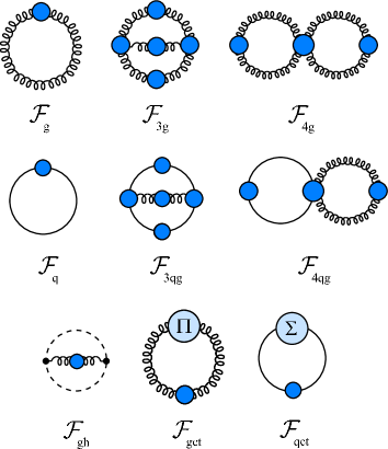
Figure 2: Diagrams contributing through NLO in HTLpt. Shaded circles indicate dressed HTL propagators and vertices.

The thermodynamic potential at next-to-leading order in HTL perturbation theory can be written as

$$\Omega_{\rm NLO} = \Omega_{\rm LO}+d_{A}\left[{\cal F}_{3g}+{\cal F}_{4g}+{\cal F}_{gh}+{\cal F}_{gct}\right]$$ (24)

$$+d_{A}s_{F}\left[{\cal F}_{3qg}+{\cal F}_{4qg}\right]+d_{f}{\cal F}_{qct}+\Delta_{1}{\cal E}_{0}$$

$$+\Delta_{1}m_{D}^{2}{\partial\over\partial m_{D}^{2}}\Omega_{\rm LO}+\Delta_{1}m_{q}^{2}{\partial\over\partial m_{q}^{2}}\Omega_{\rm LO}\;,$$

where $\Delta_{1}{\cal E}_{0}$ and $\Delta_{1}m_{D}^{2}$ are the terms of order $\delta$ in the vacuum energy density and mass counterterms. The contributions from the two-loop diagrams with the three-gluon and four-gluon vertices are

$${\cal F}_{3g} = {c_{A}\over 12}g^{2}\hbox{$\sum$}\!\!\!\!\!\!\!\int_{PQ}\Gamma^{\mu\lambda\rho}(P,Q,R)$$ (25)

$$\times\Gamma^{\nu\sigma\tau}(P,Q,R)\Delta^{\mu\nu}(P)\Delta^{\lambda\sigma}(Q)\Delta^{\rho\tau}(R)\;,$$

$${\cal F}_{4g} = {c_{A}\over 8}g^{2}\hbox{$\sum$}\!\!\!\!\!\!\!\int_{PQ}\Gamma^{\mu\nu,\lambda\sigma}(P,-P,Q,-Q)$$ (26)

$$\times\Delta^{\mu\nu}(P)\Delta^{\lambda\sigma}(Q)\;,$$

where $R=-Q-P$.

The contribution from the ghost diagram depends on the choice of gauge. The expressions in the covariant and Coulomb gauges are

$${\cal F}_{gh} = {c_{A}\over 2}g^{2}\hbox{$\sum$}\!\!\!\!\!\!\!\int_{PQ}{1\over Q^{2}}{1\over R^{2}}Q^{\mu}R^{\nu}\Delta^{\mu\nu}(P)\hskip 5.69046pt\mbox{covariant}\;,$$ (28)

$$= {c_{A}\over 2}g^{2}\hbox{$\sum$}\!\!\!\!\!\!\!\int_{PQ}{1\over q^{2}}{1\over r^{2}}\left(Q^{\mu}-Q\!\cdot\!n\;n^{\mu}\right)\left(R^{\nu}-R\!\cdot\!n\;n^{\nu}\right)$$

$$\times\Delta^{\mu\nu}(P)\hskip 93.89418pt\mbox{Coulomb}\;.$$

The contribution from the HTL gluon counterterm diagram is

$${\cal F}_{\rm gct} = {1\over 2}\hbox{$\sum$}\!\!\!\!\!\!\!\int_{P}\Pi^{\mu\nu}(P)\Delta^{\mu\nu}(P)\;.$$ (29)

The contributions from the two-loop diagrams with the quark-gluon three and four vertices are given by

$${\cal F}_{3qg} = {1\over 2}g^{2}\hbox{$\sum$}\!\!\!\!\!\!\!\int_{P\{Q\}}\mbox{Tr}\left[\Gamma^{\mu}(P,Q,R)S(Q)\right.$$ (30)

$$\left.\hskip 28.45274pt\times\Gamma^{\nu}(P,Q,R)S(R)\right]\Delta^{\mu\nu}(P)$$

$${\cal F}_{4qg} = {1\over 2}g^{2}\hbox{$\sum$}\!\!\!\!\!\!\!\int_{P\{Q\}}\mbox{Tr}\left[\Gamma^{\mu\nu}(P,-P,Q,Q)S(Q)\right]$$ (31)

$$\hskip 28.45274pt\times\Delta^{\mu\nu}(P)\;,$$

where Tr implies taking the trace over $\gamma$-matrices. The contribution from the HTL quark counterterm is

$${\cal F}_{\rm qct}=-\hbox{$\sum$}\!\!\!\!\!\!\!\int_{\{P\}}\mbox{Tr}\left[\Sigma(P)S(P)\right]\;.$$ (32)

Provided that HTL perturbation theory is renormalizable, the ultraviolet divergences at any order in $\delta$ can be cancelled by renormalizations of the vacuum energy density ${\cal E}_{0}$, the HTL mass parameters $m_{D}^{2}$ and $m_{q}^{2}$, and the coupling constant $\alpha_{s}$. Renormalization of the coupling constant does not enter until order $\delta^{2}$. We will calculate the thermodynamic potential as a double expansion in powers of $m_{D}/T$ and $m_{q}/T$, ad $g$ including all terms through 5^th order. The $\delta\alpha_{s}$ term in $\Delta{\cal E}_{0}$ does not contribute until 6^th order in this expansion, so the term of order $\delta$ in $\Delta{\cal E}_{0}$ can be obtained simply by expanding Eq. (23) to first order in $\delta$:

$$\Delta_{1}{\cal E}_{0}=-{d_{A}\over 64\pi^{2}\epsilon}m_{D}^{4}\;.$$ (33)

The remaining ultraviolet divergences must be removed by renormalization of the mass parameters $m_{D}$ and $m_{q}$. We will show below that, at order $\delta$, all remaining divergences can be removed by the quark and Debye mass counterterms. This provides nontrivial evidence for the renormalizability of HTL perturbation theory at this order in $\delta$.

The sum of the 3-gluon, 4-gluon, and ghost contributions is gauge invariant. By using the Ward identities, one can easily show that the sum of these three diagrams is independent of the gauge parameter $\xi$. With more effort, one can show the equivalence of the covariant gauge expression with $\xi=0$ and the Coulomb gauge expression with $\xi=0$. In a similar manner, it can be shown that the sum of (30) and (31) is independent of $\xi$ within the class of covariant and Coloumb gauges, as well as the equivalence of the two with $\xi=0$.

IV Reduction to scalar sum-integrals

The first step in calculating the quark contribution to the free energy is to reduce the sum of the diagrams to scalar-sum-integrals. The leading-order quark contribution can be rewritten as

$${\cal F}_{q}=-2\hbox{$\sum$}\!\!\!\!\!\!\!\int_{\{P\}}\log P^{2}-2\hbox{$\sum$}\!\!\!\!\!\!\!\int_{\{P\}}\log\left[{A_{S}^{2}-A_{0}^{2}\over P^{2}}\right]\;,$$ (34)

where

$$A_{0}(P) = iP_{0}-{m_{q}^{2}\over iP_{0}}{\cal T}_{P}\;,$$ (35)

$$A_{S}(P) = |{\bf p}|+{m^{2}_{q}\over|{\bf p}|}\left[1-{\cal T}_{P}\right]\;.$$ (36)

The HTL quark counterterm can be rewritten as

$${\cal F}_{qct}=-4\hbox{$\sum$}\!\!\!\!\!\!\!\int_{\{P\}}{P^{2}+m^{2}_{q}\over A_{S}^{2}-A_{0}^{2}}\;.$$ (37)

We proceed to simplify the sum of (30) and (31) in Landau gauge. Using the Ward identities (A.114) and (A.117) the sum of (30) and (31) becomes

$${\cal F}_{3qg+4qg} = {1\over 2}g^{2}\hbox{$\sum$}\!\!\!\!\!\!\!\int_{P\{Q\}}\Bigg{\{}\Delta_{X}(P)\mbox{Tr}\left[\Gamma^{00}S(Q)\right]-\Delta_{T}(P)\mbox{Tr}\left[\Gamma^{\mu}S(Q)\Gamma^{\mu}S(R^{\prime})\right]+\Delta_{X}(P)\mbox{Tr}\left[\Gamma^{0}S(Q)\Gamma^{0}S(R^{\prime})\right]\Bigg{\}}\;,$$ (38)

where $S$ is the quark propagator, $\Delta_{T}$ is the transverse gluon propagator, $\Delta_{X}$ is a combinaiton of the transverse and longitudinal gluon propagators defined in (A.96), and $R^{\prime}=Q-P$.

Performing the traces of $\gamma$-matrices gives

$${\cal F}_{3qg+4qg} = -g^{2}\hbox{$\sum$}\!\!\!\!\!\!\!\int_{P\{Q\}}{1\over A_{S}^{2}(Q)-A_{0}^{2}(Q)}\Bigg{\{}2(d-1)\Delta_{T}(P){\hat{\bf q}\!\cdot\!\hat{\bf r}A_{S}(Q)A_{S}(R)-A_{0}(Q)A_{0}(R)\over A_{S}^{2}(R)-A_{0}^{2}(R)}$$ (39)

$$\;\;-2\Delta_{X}(P){A_{0}(Q)A_{0}(R)+A_{S}(Q)A_{S}(R)\hat{\bf q}\!\cdot\!\hat{\bf r}\over A_{S}^{2}(R)-A_{0}^{2}(R)}-4m_{q}^{2}\Delta_{X}(P)\Bigg{\langle}{A_{0}(Q)-A_{s}(Q)\hat{{\bf q}}\!\cdot\!\hat{{\bf y}}\over(P\!\cdot\!Y)^{2}-(Q\!\cdot\!Y)^{2}}{1\over(Q\!\cdot\!Y)}\Bigg{\rangle}_{\!\!\bf\hat{y}}$$

$$\;\;+{8m_{q}^{2}\Delta_{T}(P)\over A_{S}^{2}(R)-A_{0}^{2}(R)}\Bigg{\langle}{(A_{0}(Q)-A_{S}(Q)\hat{\bf q}\!\cdot\!\hat{\bf y})(A_{0}(R)-A_{S}(R)\hat{\bf r}\!\cdot\!\hat{\bf y})\over(Q\!\cdot\!Y)(R\!\cdot\!Y)}\bigg{\rangle}_{\!\!\bf\hat{y}}$$

$$\;\;+{4m_{q}^{2}\Delta_{X}(P)\over A_{S}^{2}(R)-A_{0}^{2}(R)}\Bigg{\langle}{2A_{0}(R)A_{S}(Q)\hat{\bf q}\!\cdot\!\hat{\bf y}-A_{0}(Q)A_{0}(R)-A_{S}(Q)A_{S}(R)\hat{\bf q}\!\cdot\!\hat{\bf r}\over(Q\!\cdot\!Y)(R\!\cdot\!Y)}\Bigg{\rangle}_{\!\!\bf\hat{y}}\Bigg{\}}+O(g^{2}m_{q}^{4})\;,$$

where $A_{0}$ and $A_{S}$ are defined in (A.109) and (A.110), respectively.

V High-temperature Expansion

The free energy has been reduced to scalar sum-integrals. If we tried to evaluate the 2-loop HTL free energy exactly, there are terms that could at best be reduced to 5-dimensional integrals which would have to be evaluated numerically. We will therefore evaluate the sum-integrals approximately by expanding them in powers of $m_{D}/T$ and $m_{q}/T$. We will carry out the expansion to high enough order to include all terms through order $g^{5}$ if $m_{D}$ and $m_{q}$ are taken to be of order $g$.

The free energy can be divided into contributions from hard and soft momenta. We proceed to calculate the hard-hard and hard-soft contributions. There is no soft-soft contribution since one of the momenta in the loop is always fermionic and therefore hard.

V.1 One-loop sum-integrals

The one-loop sum-integrals include the leading quark contribution (22) and the HTL quark counterterm (32). The leading order free energy must be expanded to order $m_{q}^{4}$ to include all terms through order $g^{5}$ if $m_{q}$ is taken to be of order $g$.

V.1.1 Hard contributions

The hard contribution from the LO gluon term (21) was given in ABPS-02 and reads

$${\cal F}_{g}^{(h)} = -{\pi^{2}\over 45}T^{4}+{1\over 24}\left[1+\left(2+2{\zeta^{\prime}(-1)\over\zeta(-1)}\right)\epsilon\right]$$ (40)

$$\times\left({\mu\over 4\pi T}\right)^{2\epsilon}m_{D}^{2}T^{2}-{1\over 128\pi^{2}}\left({1\over\epsilon}-7+2\gamma+{2\pi^{2}\over 3}\right)$$

$$\times\left({\mu\over 4\pi T}\right)^{2\epsilon}m_{D}^{4}\,.$$

The hard contribution from the HTL counterterm (29) was given in ABPS-02 and reads

$${\cal F}_{gct}^{(h)} = -{1\over 24}m_{D}^{2}T^{2}+{1\over 64\pi^{2}}\left({1\over\epsilon}-7+2\gamma+{2\pi^{2}\over 3}\right)$$ (41)

$$\times\left({\mu\over 4\pi T}\right)^{2\epsilon}m_{D}^{4}\,.$$

The sum-integrals over $P$ involve two momentum scales $m_{q}$ and $T$. Since $P_{0}=(2n+1)\pi T$, the momentum is always hard. We can therefore expand in powers of $m_{q}^{2}$. To second order in $m_{q}^{2}$, we obtain

$${\cal F}^{(h)}_{q} = -2\hbox{$\sum$}\!\!\!\!\!\!\!\int_{\{P\}}\log P^{2}-4m_{q}^{2}\hbox{$\sum$}\!\!\!\!\!\!\!\int_{\{P\}}{1\over P^{2}}$$ (42)

$$+2m_{q}^{4}\hbox{$\sum$}\!\!\!\!\!\!\!\int_{\{P\}}\left[{2\over P^{4}}-{1\over p^{2}P^{2}}+{2\over p^{2}P^{2}}{\cal T}_{P}-{1\over p^{2}P_{0}^{2}}\left({\cal T}_{P}\right)^{2}\right]\;.$$

Note that the function ${\cal T}_{P}$ cancels from the $m_{q}^{2}$ term. The values of the sum-integrals are given in Appendix B. Inserting those expressions, the hard quark contributions to the free energy reduce to

$${\cal F}_{q}^{(h)} = -{7\pi^{2}\over 180}T^{4}+{1\over 6}\left[1+\left(2-2\log 2+2{\zeta^{\prime}(-1)\over\zeta(-1)}\right)\epsilon\right]$$ (43)

$$\times\left({\mu\over 4\pi T}\right)^{2\epsilon}m_{q}^{2}T^{2}+{1\over 12\pi^{2}}\left(\pi^{2}-6\right)m_{q}^{4}\;.$$

Note that this contribution is finite and so the leading order counterterm $\Delta_{0}{\cal E}_{0}$ is the same as in the pure-glue case. The HTL quark counterterm is given in (37). Expanding this term to second order in $m_{q}^{2}$ yields

$${\cal F}^{(h)}_{\rm qct} = 4m_{q}^{2}\hbox{$\sum$}\!\!\!\!\!\!\!\int_{\{P\}}{1\over P^{2}}-4m_{q}^{4}\hbox{$\sum$}\!\!\!\!\!\!\!\int_{\{P\}}\left[{2\over P^{4}}-{1\over p^{2}P^{2}}\right.$$ (44)

$$\left.+{2\over p^{2}P^{2}}{\cal T}_{P}-{1\over p^{2}P_{0}^{2}}\left({\cal T}_{P}\right)^{2}\right]\;.$$

The values of the sum-integrals are given in Appendix B. Inserting those expressions, the hard contributions to the HTL quark counterterm reduce to

$${\cal F}^{(h)}_{\rm qct}=-{1\over 6}m_{q}^{2}T^{2}-{1\over 6\pi^{2}}\left(\pi^{2}-6\right)m_{q}^{4}\;.$$ (45)

Note that the first term in Eq. (45) cancels the order-$\epsilon^{0}$ term in coefficient of $m_{q}^{2}$ in Eq. (43)

V.1.2 Soft contributions

The soft contribution comes from the $P_{0}=0$ term in the sum-integral. At soft momentum $P=(0,{\bf p})$, the HTL self-energy functions reduce to $\Pi_{T}(P)=0$ and $\Pi_{L}(P)=m_{D}^{2}$. The transverse term vanishes in dimensional regularization because there is no momentum scale in the integral over ${\bf p}$. Thus the soft contribution comes from the longitudinal term only.

The soft contribution to the leading order free energy (21) was given in Ref. ABPS-02 and reads

$${\cal F}_{g}^{(s)} = -{1\over 12\pi}\left[1+{8\over 3}\epsilon\right]\left({\mu\over 2m_{D}}\right)^{2\epsilon}m_{D}^{3}T\,.$$ (46)

The soft contribution to the HTL gluon counterterm (29) given in Ref. ABPS-02 and reads

$${\cal F}_{gct}^{(s)} = {1\over 8\pi}m_{D}^{3}T\,.$$ (47)

There are no soft contribution from the leading-order quark term (34) or from the HTL quark counterterm (37).

V.2 Two-loop sum-integrals

The sum of the two-loop sum-integrals is given in (38). Since these integrals have an explicit factor of $g^{2}$, we need only to expand the sum-integrals to order $m_{q}^{2}m_{D}/T^{3}$ and $m_{D}^{3}/T^{3}$ to include all terms through order $g^{5}$.

The sum-integrals involve two momentum scales $m_{q},m_{D}$ and $T$. In order to expand them in powers of.., we separate them into contributions from hard loop momenta and soft loop momenta. This gives two separate regions which we will denote $(hh)$ and $(hs)$. In the $(hh)$ region, all three momenta $P$, $Q$, and $R$ are hard. In the $(hs)$ region, two of the three momenta are hard and the other soft.

V.2.1 Contributions from the (hh) region

For hard momenta, the self-energies are suppressed by $m_{D}^{2}/T^{2}$ or $m_{q}^{2}/T^{2}$ relative to the propagators, so we can expand in powers of $\Pi_{T}$, $\Pi_{L}$, and $\Sigma$.

The $(hh)$ contribution from (25)–(28) was given in Ref. ABPS-02 and reads

$${\cal F}_{3g+4g+gh}^{(hh)} = {\pi^{2}\over 12}{c_{A}\alpha_{s}\over 3\pi}T^{4}\;-\;{7\over 96}\left[{1\over\epsilon}+4.621\right]{c_{A}\alpha_{s}\over 3\pi}$$ (48)

$$\left({\mu\over 4\pi T}\right)^{4\epsilon}m_{D}^{2}T^{2}\,.$$

The $(hh)$ contribution from (30) and (31) can be written as

$${\cal F}_{3qg+4qg}^{(hh)} = (d-1)g^{2}\left[\hbox{$\sum$}\!\!\!\!\!\!\!\int_{\{PQ\}}{1\over P^{2}Q^{2}}-\hbox{$\sum$}\!\!\!\!\!\!\!\int_{P\{Q\}}{2\over P^{2}Q^{2}}\right]+2m_{D}^{2}g^{2}\hbox{$\sum$}\!\!\!\!\!\!\!\int_{P\{Q\}}\left[{1\over p^{2}P^{2}Q^{2}}{\cal T}_{P}+{1\over(P^{2})^{2}Q^{2}}-{d-2\over d-1}{1\over p^{2}P^{2}Q^{2}}\right]$$ (49)

$$+m_{D}^{2}g^{2}\hbox{$\sum$}\!\!\!\!\!\!\!\int_{\{PQ\}}\left[{d+1\over d-1}{1\over P^{2}Q^{2}r^{2}}-{4d\over d-1}{q^{2}\over P^{2}Q^{2}r^{4}}-{2d\over d-1}{P\!\cdot\!Q\over P^{2}Q^{2}r^{4}}\right]{\cal T}_{R}$$

$$+m_{D}^{2}g^{2}\hbox{$\sum$}\!\!\!\!\!\!\!\int_{\{PQ\}}\left[{3-d\over d-1}{1\over P^{2}Q^{2}R^{2}}+{2d\over d-1}{P\!\cdot\!Q\over P^{2}Q^{2}r^{4}}-{d+2\over d-1}{1\over P^{2}Q^{2}r^{2}}+{4d\over d-1}{q^{2}\over P^{2}Q^{2}r^{4}}-{4\over d-1}{q^{2}\over P^{2}Q^{2}r^{2}R^{2}}\right]$$

$$+2m_{q}^{2}g^{2}(d-1)\hbox{$\sum$}\!\!\!\!\!\!\!\int_{\{PQ\}}\left[{1\over P^{2}Q_{0}^{2}Q^{2}}+{p^{2}-r^{2}\over P^{2}q^{2}Q_{0}^{2}R^{2}}\right]{\cal T}_{Q}+2m_{q}^{2}g^{2}(d-1)\hbox{$\sum$}\!\!\!\!\!\!\!\int_{P\{Q\}}\left[{2\over P^{2}(Q^{2})^{2}}-{1\over P^{2}Q_{0}^{2}Q^{2}}{\cal T}_{Q}\right]$$

$$+2m_{q}^{2}g^{2}(d-1)\hbox{$\sum$}\!\!\!\!\!\!\!\int_{\{PQ\}}\left[{d+3\over d-1}{1\over P^{2}Q^{2}R^{2}}-{2\over P^{2}(Q^{2})^{2}}+{r^{2}-p^{2}\over q^{2}P^{2}Q^{2}R^{2}}\right].$$

Using the expressions for the sum-integrals in Appendix B, this reduces to

$${\cal F}_{3qg+4qg} = {5\pi^{2}\over 72}{\alpha_{s}\over\pi}T^{4}-{1\over 72}\left[{1\over\epsilon}+1.2963\right]{\alpha_{s}\over\pi}\left({\mu\over 4\pi T}\right)^{4\epsilon}m_{D}^{2}T^{2}+{1\over 8}\left[{1\over\epsilon}+8.96751\right]{\alpha_{s}\over\pi}\left({\mu\over 4\pi T}\right)^{4\epsilon}m_{q}^{2}T^{2}\;.$$ (50)

V.2.2 The (hs) contribution

In the $(hs)$ region, the momentum $P$ is soft. The momenta $Q$ and $R$ are always hard. The function that multiplies the soft propagator $\Delta_{T}(0,{\bf p})$ or $\Delta_{X}(0,{\bf p})$ can be expanded in powers of the soft momentum ${\bf p}$. In the case of $\Delta_{T}(0,{\bf p})$, the resulting integrals over ${\bf p}$ have no scale and they vanish in dimensional regularization. The integration measure $\int_{\bf p}$ scales like $m_{D}^{3}$, the soft propagator $\Delta_{X}(0,{\bf p})$ scales like $1/m_{D}^{2}$, and every power of $p$ in the numerator scales like $m_{D}$.

The $(hs)$ contribution from (25)–(28) was given in Ref. ABPS-02 and reads

$${\cal F}_{3g+4g+gh}^{(hs)} = -{\pi\over 2}{c_{A}\alpha_{s}\over 3\pi}m_{D}T^{3}\;-\;{11\over 32\pi}\left({1\over\epsilon}+{27\over 11}+2\gamma\right){c_{A}\alpha_{s}\over 3\pi}\left({\mu\over 4\pi T}\right)^{2\epsilon}\left({\mu\over 2m_{D}}\right)^{2\epsilon}m_{D}^{3}T\,.$$ (51)

The only terms that contribute through order $g^{2}m_{D}^{3}T$ and $m_{q}^{2}m_{D}g^{3}T$ from  (30) and (31) are

$${\cal F}_{3qg+4qg}^{(hs)} = g^{2}T\int_{\bf p}{1\over p^{2}+m^{2}_{D}}\hbox{$\sum$}\!\!\!\!\!\!\!\int_{\{Q\}}\left[{2\over Q^{2}}-{4q^{2}\over(Q^{2})^{2}}\right]+2m_{D}^{2}g^{2}T\int_{\bf p}{1\over p^{2}+m_{D}^{2}}\hbox{$\sum$}\!\!\!\!\!\!\!\int_{\{Q\}}\left[{1\over(Q^{2})^{2}}-(3+d){2\over d}{q^{2}\over(Q^{2})^{3}}+{8\over d}{q^{4}\over(Q^{2})^{4}}\right]$$ (52)

$$-4m_{q}^{2}g^{2}T\int_{\bf p}{1\over p^{2}+m_{D}^{2}}\hbox{$\sum$}\!\!\!\!\!\!\!\int_{\{Q\}}\left[{3\over(Q^{2})^{2}}-{4q^{2}\over(Q^{2})^{3}}-{4\over(Q^{2})^{2}}{\cal T}_{Q}-{2\over Q^{2}}\bigg{\langle}{1\over(Q\!\cdot\!Y)^{2}}\bigg{\rangle}_{\!\!\bf\hat{y}}\right]\;.$$

In the terms that are already of order $g^{2}m_{D}^{3}T$, we can set $R=-Q$. In the terms of order $g^{2}m_{D}T^{3}$, we must expand the sum-integrand to second order in ${\bf p}$. After averaging over angles of ${\bf p}$, the linear terms in ${\bf p}$ vanish and quadratic terms of the form $p^{i}p^{j}$ are replaced by $p^{2}\delta^{ij}/d$. We can set $p^{2}=-m_{D}^{2}$, because any factor proportional to $p^{2}+m_{D}^{2}$ will cancel the denominator of the integral over ${\bf p}$, leaving an integral with no scale. This gives

$${\cal F}_{3qg+4qg}^{(hs)} = -{1\over 6}\alpha_{s}m_{D}T^{3}+{\alpha_{s}\over 24\pi^{2}}\left[{1\over\epsilon}+1+2\gamma+4\log 2\right]$$

$$\times\left({\mu\over 4\pi T}\right)^{2\epsilon}\left({\mu\over 2m_{D}}\right)^{2\epsilon}m_{D}^{3}T-{\alpha_{s}\over 2\pi^{2}}m_{q}^{2}m_{D}T\;.$$

V.2.3 The $(ss)$ contributions

The $(ss)$ contribution from (25)–(28) was given in Ref. ABPS-02 and reads

$${\cal F}_{3g+4g+gh}^{(ss)} = {3\over 16}\left[{1\over\epsilon}+3\right]{c_{A}\alpha_{s}\over 3\pi}\left({\mu\over 2m_{D}}\right)^{4\epsilon}m_{D}^{2}T^{2}\,.$$ (54)

There is no $(ss)$ contribution from the diagrams involving fermions.

VI HTL-Improved Thermodynamics

The free energy at second order in HTL perturbation theory defines a function $\Omega(T,\alpha_{s},m_{D},m_{q},\delta=1)$. We will refer to this function as the thermodynamic potential. To obtain the free energy $F(T)$ as a function of the temperature, we need to specify a prescription for the mass parameter $m_{D}$ as a function of $T$ and $\alpha_{s}$.

VII Thermodynamic Potential

In this section, we calculate the thermodynamic potential $\Omega(T,\alpha_{s},m_{D},m_{q},\delta=1)$ explicitly, first to leading order in the $\delta$ expansion and then to next-to-leading order.

VII.1 Leading order

The complete expression for the leading order thermodynamic potential is the sum of the contributions from 1-loop diagrams and the leading term (23) in the vacuum energy counterterm. The contributions from the 1-loop diagrams, including all terms through order $g^{5}$, is the sum of (40), (43), and (46)

$$\Omega_{1-{\rm loop}} = -d_{A}{\pi^{2}T^{4}\over 45}\left\{1+{7\over 4}{d_{F}\over d_{A}}-{15\over 2}\hat{m}_{D}^{2}-30{d_{F}\over d_{A}}\hat{m}_{q}^{2}\right.$$ (55)

$$\left.+30\hat{m}_{D}^{3}+{45\over 8}\left({1\over\epsilon}+2\log{\hat{\mu}\over 2}-7+2\gamma+{2\pi^{2}\over 3}\right)\hat{m}_{D}^{4}\right.$$

$$\left.-60{d_{F}\over d_{A}}\left(\pi^{2}-6\right)\hat{m}_{q}^{4}\right\}\;,$$

where $\hat{m}_{D}$, $\hat{m}_{q}$ and $\hat{\mu}$ are dimensionless variables:

$$\hat{m}_{D} = {m_{D}\over 2\pi T}\;,$$ (56)

$$\hat{m}_{q} = {m_{q}\over 2\pi T}\;,$$ (57)

$$\hat{\mu} = {\mu\over 2\pi T}\;.$$ (58)

Adding the counterterm (23), we obtain the thermodynamic potential at leading order in the delta expansion:

$$\Omega_{\rm LO} = -d_{A}{\pi^{2}T^{4}\over 45}\left\{1+{7\over 4}{d_{F}\over d_{A}}-{15\over 2}\hat{m}_{D}^{2}-30{d_{F}\over d_{A}}\hat{m}_{q}^{2}\right.$$ (59)

$$\left.+30\hat{m}_{D}^{3}+{45\over 4}\left(\log{\hat{\mu}\over 2}-{7\over 2}+\gamma+{\pi^{2}\over 3}\right)\hat{m}_{D}^{4}\right.$$

$$\left.-60{d_{F}\over d_{A}}\left(\pi^{2}-6\right)\hat{m}_{q}^{4}\right\}\;,$$

VII.2 Next-to-leading order

The complete expression for the next-to-leading order correction to the thermodynamic potential is the sum of the contributions from all 2-loop diagrams, the quark and gluon counterterms, and renormalization counterterms. The contributions from the 2-loop diagrams, including all terms though order $g^{5}$ is the sum of (48), (50), (51), (LABEL:F2loop-qhs), and (54) multiplied by the appropriate group structure constants listed in (24):

$$\Omega_{\rm 2-loop} = -d_{A}{\pi^{2}T^{4}\over 45}{\alpha_{s}\over\pi}\Bigg{\{}-{5\over 4}\left(c_{A}+{5\over 2}s_{F}\right)+15(c_{A}+s_{F})\hat{m}_{D}-{55\over 8}\bigg{[}\left(c_{A}-{4\over 11}s_{F}\right)\left({1\over\epsilon}+4\log{\hat{\mu}\over 2}\right)$$ (60)

$$-c_{A}\left({72\over 11}\log\hat{m}_{D}-1.96869\right)-0.4714\,s_{F}\bigg{]}\hat{m}_{D}^{2}-{45\over 2}s_{F}\left[{1\over\epsilon}+4\log{\hat{\mu}\over 2}+8.96751\right]\hat{m}_{q}^{2}+180\,s_{F}\hat{m}_{D}\hat{m}_{q}^{2}$$

$$+{165\over 4}\bigg{[}\left(c_{A}-{4\over 11}s_{F}\right)\left({1\over\epsilon}+4\log{\hat{\mu}\over 2}-2\log\hat{m}_{D}\right)+c_{A}\left({27\over 11}+2\gamma\right)-{4\over 11}s_{F}\left(1+2\gamma+4\log 2\right)\bigg{]}\hat{m}_{D}^{3}\Bigg{\}}\;.$$

The HTL gluon counterterm is the sum of (41) and (47)

$$\Omega_{\rm gct} = -d_{A}{\pi^{2}T^{4}\over 45}\left\{{15\over 2}\hat{m}_{D}^{2}-45\hat{m}_{D}^{3}-{45\over 4}\left({1\over\epsilon}+2\log{\hat{\mu}\over 2}-7+2\gamma+{2\pi^{2}\over 3}\right)\hat{m}_{D}^{4}\right\}\;.$$ (61)

The HTL quark counterterm is given by (45)

$$\Omega_{\rm qct} = -d_{F}{\pi^{2}T^{4}\over 45}\left\{30\hat{m}_{q}^{2}+120\left(\pi^{2}-6\right)\hat{m}_{q}^{4}\right\}\;.$$ (62)

The ultraviolet divergences that remain after these 3 terms are added can be removed by renormalization of the vacuum energy density ${\cal E}_{0}$ and the HTL mass parameter $m_{D}$. The renormalization contributions at first order in $\delta$ are

$$\Delta\Omega\;=\;\Delta_{1}{\cal E}_{0}+\Delta_{1}m_{D}^{2}{\partial\ \ \over\partial m_{D}^{2}}\Omega_{\rm LO}+\Delta_{1}m_{q}^{2}{\partial\ \ \over\partial m_{q}^{2}}\Omega_{\rm LO}\;.$$ (63)

Using the results listed in Eqs. (17), (18), and (33) the complete contribution from the counterterm at first order in $\delta$ is

$$\Delta\Omega = -d_{A}{\pi^{2}T^{4}\over 45}\Bigg{\{}{45\over 4\epsilon}\hat{m}_{D}^{4}+{\alpha_{s}\over\pi}\Bigg{[}{55\over 8}\left(c_{A}-{4\over 11}s_{F}\right)\left({1\over\epsilon}+2\log{\hat{\mu}\over 2}+2{\zeta^{\prime}(-1)\over\zeta(-1)}+2\right)\hat{m}_{D}^{2}$$

$$-{165\over 4}\left(c_{A}-{4\over 11}s_{F}\right)\left({1\over\epsilon}+2\log{\hat{\mu}\over 2}-2\log\hat{m}_{D}+2\right)\hat{m}_{D}^{3}+{45\over 2}s_{F}\left({1\over\epsilon}+2+2\log{\hat{\mu}\over 2}-2\log 2+2{\zeta^{\prime}(-1)\over\zeta(-1)}\right)\hat{m}_{q}^{2}\Bigg{]}\Bigg{\}}\;.$$

Adding the contributions from the two-loop diagrams in (60), the HTL gluon and quark counterterms in (61) and (62), the contribution from vacuum and mass renormalizations in (LABEL:OmegaVMct), and the leading order thermodynamic potential in (59) we obtain the complete expression for the QCD thermodynamic potential at next-to-leading order in HTLpt:

$$\Omega_{\rm NLO} = -d_{A}{\pi^{2}T^{4}\over 45}\Bigg{\{}1+{7\over 4}{d_{F}\over d_{A}}-15\hat{m}_{D}^{3}-{45\over 4}\left(\log\hat{\mu\over 2}-{7\over 2}+\gamma+{\pi^{2}\over 3}\right)\hat{m}_{D}^{4}+60{d_{F}\over d_{A}}\left(\pi^{2}-6\right)\hat{m}_{q}^{4}$$ (65)

$$+{\alpha_{s}\over\pi}\Bigg{[}-{5\over 4}\left(c_{A}+{5\over 2}s_{F}\right)+15\left(c_{A}+s_{F}\right)\hat{m}_{D}-{55\over 4}\bigg{\{}c_{A}\left(\log{\hat{\mu}\over 2}-{36\over 11}\log\hat{m}_{D}-2.001\right)-{4\over 11}s_{F}\left(\log{\hat{\mu}\over 2}-2.337\right)\!\!\bigg{\}}\hat{m}_{D}^{2}$$

$$-45\,s_{F}\left(\log{\hat{\mu}\over 2}+2.192\right)\hat{m}_{q}^{2}+{165\over 2}\bigg{\{}c_{A}\left(\log{\hat{\mu}\over 2}+{5\over 22}+\gamma\right)-{4\over 11}s_{F}\left(\log{\hat{\mu}\over 2}-{1\over 2}+\gamma+2\log 2\right)\!\!\bigg{\}}\hat{m}_{D}^{3}+180\,s_{F}\hat{m}_{D}\hat{m}_{q}^{2}\Bigg{]}\Bigg{\}}\;.$$

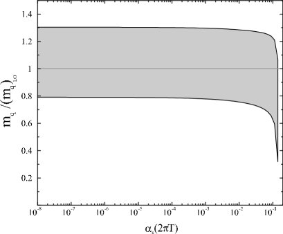
Figure 3: Numerical solution of gap equations for (a) $m_{D}$ (69) and (b) $m_{q}$ (68) as a function of $\alpha_{s}(2\pi T)$ for $N_{c}=3$ and $N_{f}=3$. The shaded band corresponds to varying the renormalization scale $\mu$ by a factor of two around $\mu=2\pi T$.

VII.3 Gap Equation

The quark and gluon mass parameters, $m_{q}$ and $m_{D}$, are determined variationally by requiring that the derivative of $\Omega_{\rm NLO}$ with respect to each parameter taken holding the other constant vanishes

$${\partial\over\partial m_{q}}\Omega_{\rm NLO}(T,\alpha_{s},m_{D},m_{q}) = 0\;,$$ (66)

$${\partial\over\partial m_{D}}\Omega_{\rm NLO}(T,\alpha_{s},m_{D},m_{q}) = 0\;.$$ (67)

The first equation above results in the following equation for $m_{q}$

$$8{d_{F}\over d_{A}}(\pi^{2}-6)\hat{m}_{q}^{2}={\alpha_{s}s_{F}\over\pi}\Bigg{[}3\left(\log{\hat{\mu}\over 2}+2.192\right)-12\hat{m}_{D}\Bigg{]}\,.$$ (68)

In the limit of small $\alpha_{s}$ the above gap equation does not go to the perturbative limit for the quark mass which is $\hat{m}_{q,\rm pert}^{2}=c_{F}\,\alpha_{s}/8\pi$. The fact that $m_{q}$ does not go to the perturbative value in the small $\alpha_{s}$ limit is due to the fact that the perturbative limit of the quark gap equation results from terms which are $O(\alpha_{s}^{2})$ and these terms are not included completely at NLO in HTLpt. One might hope that going to the next order in HTLpt would cure this problem; however, this will in fact not happen since the fermion sector is infrared safe and therefore only even powers of $\hat{m}_{q}$ will appear at each order. At NNLO all terms contributing at $O(\alpha_{s}^{2})$ at NLO will be replaced by explicit powers of $\alpha_{s}$ and all $\hat{m}_{q}$ dependence will be pushed up to $O(\alpha_{s}^{3})$. This behavior will persist at all orders in HTLpt so that at any order the weak-coupling limit of the gap equation quark mass will be scale dependent. In order to circumvent this problem we can consider other possible prescriptions for choosing $\hat{m}_{q}$ which include requiring that $\hat{m}_{q}$ be equal to its perturbative value for all $\alpha_{s}$ or requiring that $\hat{m}_{q}$ be proportional to $\hat{m}_{D}$ with the proportionality constant fixed in the weak-coupling limit.

Performing the derivative with respect to $m_{D}$ while holding $m_{q}$ fixed results in the following gap equation for $m_{D}$

$$45\hat{m}_{D}^{2}\left[1+\left(\log\hat{\mu\over 2}-{7\over 2}+\gamma+{\pi^{2}\over 3}\right)\hat{m}_{D}\right]$$

$$={\alpha\over\pi}\Bigg{\{}15\left(c_{A}+s_{F}\right)-{55\over 2}\bigg{[}c_{A}\left(\log{\hat{\mu}\over 2}-{36\over 11}\log\hat{m}_{D}-3.637\right)$$

$$-{4\over 11}s_{F}\left(\log{\hat{\mu}\over 2}-2.337\right)\!\!\bigg{]}\hat{m}_{D}+{495\over 2}\bigg{[}c_{A}\left(\log{\hat{\mu}\over 2}+{5\over 22}+\gamma\right)$$

$$-{4\over 11}s_{F}\left(\log{\hat{\mu}\over 2}-{1\over 2}+\gamma+2\log 2\right)\!\!\bigg{]}\hat{m}_{D}^{2}+180\,s_{F}\hat{m}_{q}^{2}\Bigg{\}}\;.$$ (69)

The last term in Eq. (69) proportional to $\hat{m}_{q}^{2}$ can be written in terms of $\hat{m}_{D}$ using Eq. (68). In Fig. 3 we plot the solutions to the gap equations for $m_{D}$ and $m_{q}$ for $N_{c}=3$ and $N_{f}=2$. The solution for $m_{D}$ goes to the perturbative value in the limit of small $\alpha_{s}$, decreases below the perturbative value as $\alpha_{s}$ increases, and becomes larger than the perturbative value at $\alpha_{s}\sim 0.11$. The solution for $m_{q}$ does not go to the perturbative value in the limit of small $\alpha_{s}$ and is instead scale dependent even at lowest order as dicussed above. As $\alpha_{s}$ increases the value of $m_{q}$ remains very flat regardless of the scale, changing significantly only near $\alpha_{s}\sim 0.10$.

VIII Free energy

The free energy is obtained by evaluating the leading and next-to-leading order thermodynamic potentials, (59) and (65), at the solution to the gap equations (68) and (69). In Fig. 4 we plot the leading and next-to-leading order HTLpt predictions for the free energy of QCD with $N_{c}=3$ and $N_{f}=2$. We have studied the alternative prescriptions for the quark mass discussed in the previous section and find that the NLO free energy obtained using these prescriptions is numerically indistinguishable from that obtained using the quark gap equations. As can be seen from this figure the corrections in going from LO to NLO are small over the entire temperature range, especially when compared to convergence of the perturbative result. Additionally, the scale variation of the NLO HTLpt result for the free energy is much smaller than the LO showing that the partial resummation of the scale dependent logarithms reduces the scale variation of the final results significantly.

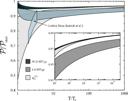
Figure 4: LO and NLO HTLpt predictions for the free energy of QCD with $N_{c}=3$ and $N_{f}=2$ together with the perturbative prediction accurate to $g^{5}$. The shaded bands correspond to varying the renormalization scale $\mu$ by a factor of two around $\mu=2\pi T$. Also shown is a lattice estimate by Karsch et al. klp for the free energy. The band indicates the estimated systematic error of their result which is reported as (15$\pm$5)%.

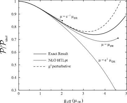
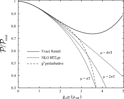
Figure 5: NLO HTLpt prediction for the $O(N_{f}^{0})$ contribution to the free energy, the numerical result of Ref. ipp , and the perturbative prediction accurate to $g^{5}$ as a function of $g_{\rm eff}(\mu_{\rm DR})=\sqrt{s_{f}}g(\mu_{\rm DR})=2\pi\sqrt{s_{f}\alpha_{s}(\mu_{\rm DR})}$ where $\mu_{\rm DR}=\pi e^{-\gamma}T$. Dots indicate the point at which there is no longer a real-valued solution to the gap equation for $m_{D}$. In (a) the renormalization scale $\mu$ is varied by a factor of $e$ around $\mu_{\rm DR}$. In (b) the renormalization scale $\mu$ is varied by a factor of $2$ around $2\pi T$. In both (a) and (b) the perturbative $g^{5}$ result is evaluated at the central scale.

However, as was the case in pure-glue QCD ABPS-02 , the results seem to lie significantly above the lattice data which is available below $5\,T_{c}$. There are several reasons for why HTLpt might fail to describe the lattice data in this temperature range. One is that the hard modes are not resummed properly within HTLpt and that a description using a $\Phi$-derivable approach which explicitly separates the hard and soft modes as done in Ref. BIR-99 is better. A second is that HTLpt discards some important physics like topological modes or the $Z_{N}$ symmetry of QCD near the phase transition.

A third possibility is that the expansion in $m_{D}/T$ and $m_{q}/T$ breaks down at these temperatures. Numerically, $m_{D}/T\sim 1.2$ and $m_{q}/T\sim 0.5$ at $5\,T_{c}$ and $m_{D}/T\sim 1.6$ and $m_{q}/T\sim 0.6$ at $2\,T_{c}$, which casts doubt on the applicability of the expansion in this temperature range. However, in the case of pure-glue we have been able to compare the LO HTLpt result expanded to $O(\hat{m}_{D}^{6})$ with the non-truncated LO expression which is accurate to all orders in $\hat{m}_{D}$ and find that the expansions converge very rapidly. Numerically we find that at $m_{D}/T=5$ truncations of the LO order result accurate to $\hat{m}_{D}^{4}$ and $\hat{m}_{D}^{6}$ reproduce the exact result to 5% and 0.2%, respectively. There have also been studies of the convergence of the mass expansions of the three-loop free energy for a massless scalar field theory using screened perturbation theory AS-01 and the $\Phi$-derivable approach BP-01 which demonstrated that mass expansions also converge very rapidly at NLO and NNLO. This gives us some confidence that the truncated NLO solutions are numerically reliable.

Figure 6: NLO HTLpt prediction for $m_{D}$ in the large $N_{f}$ limit and the exact numerical result tonyprivate as a function of $g_{\rm eff}(\mu_{\rm DR})=\sqrt{s_{f}}g(\mu_{\rm DR})=2\pi\sqrt{s_{f}\alpha_{s}(\mu_{\rm DR})}$ where $\mu_{\rm DR}=\pi e^{-\gamma}T$. In (a) the renormalization scale $\mu$ is varied by a factor of $e$ around $\mu_{\rm DR}$. In (b) the renormalization scale $\mu$ is varied by a factor of $2$ around $2\pi T$.

IX Large $N_{f}$

In the limit that $N_{f}$ is taken large while holding $g^{2}N_{f}$ fixed it is possible to solve for the $O(N_{f}^{0})$ contribution to the free energy exactly moore ; ipp . In Fig. 5 we plot the NLO HTLpt prediction for the $O(N_{f}^{0})$ contribution to the free energy along with the numerical result of Ref. ipp and the perturbative prediction which is accurate to $O(\alpha_{s}^{5/2})$. In Fig. 6 we plot the NLO HTLpt prediction for $m_{D}$ in the large $N_{f}$ limit and the exact numerical result tonyprivate . The HTLpt predictions for both the free energy and the Debye mass seem diverge from the exact result around $g_{\rm eff}\sim 2$ regardless of the scale which is chosen; however, for both quantities, choosing the scale to be $\mu=\mu_{\rm DR}=\pi e^{-\gamma}T$ seems to provide a reasonable reproduction of the exact results. This result is comparable to the performance of the $\Phi$-derivable approach in the large $N_{f}$ limit rebhan-03 .

X Conclusions

In this paper we have extended our previous HTLpt calculation of the thermodynamic functions in pure-glue QCD to include the contribution of $N_{f}$ massless quarks. We have presented results for the leading- and next-to-leading-order HTLpt predictions for the QCD free energy for arbitrary $N_{f}$. Using the NLO HTLpt expression for the thermodynamic potential we were able to find variational solutions for both the quark and gluon mass parameters allowing a first-principles prediction of the QCD free energy. As in the case of pure-glue we find that the NLO HTLpt prediction lies significantly above the available lattice data below $5\,T_{c}$; however, the problem of oscillation of successive approximations and large scale dependence of the perturbative results is eliminated by using this reorganization.

The failure of HTLpt to describe the lattice data in this region could be attributed to the failure of the expansion performed in $\hat{m}_{D}$ and $\hat{m}_{q}$; however, a study of the convergence of the truncated LO expressions to a numerical evaluation of the exact LO expression shows that these expansions converge very rapidly. Therefore, we are steered towards the conclusion that a systematic description of QCD thermodynamics using HTLpt is not appropriate below $5\,T_{c}$. The $\Phi$-derivable approach seems to agree better with the lattice data in this range so perhaps HTLpt is not resumming the hard modes properly and an explicit separation of hard and soft scales is required. However, we should point out that some authors believe that a description of QCD thermodynamics near the phase transition in terms of Polyakov loops is necessary pisarski-00 .

We have also compared the NLO HTLpt free energy and Debye mass with exact results which are available in the large $N_{f}$ limit. This comparison shows that, in the large $N_{f}$ limit, NLO HTLpt agrees with the exact result only out to $g_{\rm eff}\sim 2$ and has large scale dependence after this point. The large scale dependence is not surprising given the fact that in the large $N_{f}$ limit the running of the coupling constant is driven by the presence of the Landau singularity and even the exact results are sensitive to this beyond $g_{\rm eff}\sim 5$. The poor performance of NLO HTLpt, however, is comparable to recent large $N_{f}$ predictions within the $\Phi$-derivable approach. The failure of both approaches to agree better with the exact result for large values of $g_{\rm eff}$ is an indication that a description of strongly-coupled QCD thermodynamics solely in terms of HTL quasiparticles is perhaps inappropriate. However, it is possible that the physics of large-$N_{f}$ QCD is so different from that of QCD with a small number of flavors that it cannot serve as a definitive testing ground for the applicability of the quasiparticle approach to the physical case peshier-03 .

Appendix A HTL Feynman Rules

In this appendix, we present Feynman rules for HTL perturbation theory in QCD. We give explicit expressions for the propagators and for the quark-gluon 3 and 4 vertices. The Feynman rules are given in Minkowski space to facilitate applications to real-time processes. A Minkowski momentum is denoted $p=(p_{0},{\bf p})$, and the inner product is $p\cdot q=p_{0}q_{0}-{\bf p}\cdot{\bf q}$. The vector that specifies the thermal rest frame is $n=(1,{\bf 0})$.

A.1 Gluon Self-energy

The HTL gluon self-energy tensor for a gluon of momentum $p$ is

$$\Pi^{\mu\nu}(p)=m_{D}^{2}\left[{\cal T}^{\mu\nu}(p,-p)-n^{\mu}n^{\nu}\right]\;.$$ (A.70)

The tensor ${\cal T}^{\mu\nu}(p,q)$, which is defined only for momenta that satisfy $p+q=0$, is

$${\cal T}^{\mu\nu}(p,-p)=\left\langle y^{\mu}y^{\nu}{p\!\cdot\!n\over p\!\cdot\!y}\right\rangle_{\bf\hat{y}}\;.$$ (A.71)

The angular brackets indicate averaging over the spatial directions of the light-like vector $y=(1,\hat{\bf y})$. The tensor ${\cal T}^{\mu\nu}$ is symmetric in $\mu$ and $\nu$ and satisfies the “Ward identity”

$$p_{\mu}{\cal T}^{\mu\nu}(p,-p)=p\!\cdot\!n\;n^{\nu}\;.$$ (A.72)

The self-energy tensor $\Pi^{\mu\nu}$ is therefore also symmetric in $\mu$ and $\nu$ and satisfies

$$p_{\mu}\Pi^{\mu\nu}(p) = 0\;,$$ (A.73)

$$g_{\mu\nu}\Pi^{\mu\nu}(p) = -m_{D}^{2}\;.$$ (A.74)

The gluon self-energy tensor can be expressed in terms of two scalar functions, the transverse and longitudinal self-energies $\Pi_{T}$ and $\Pi_{L}$, defined by

$$\Pi_{T}(p) = {1\over d-1}\left(\delta^{ij}-\hat{p}^{i}\hat{p}^{j}\right)\Pi^{ij}(p)\;,$$ (A.75)

$$\Pi_{L}(p) = -\Pi^{00}(p)\;,$$ (A.76)

where ${\bf\hat{p}}$ is the unit vector in the direction of ${\bf p}$. In terms of these functions, the self-energy tensor is

$$\Pi^{\mu\nu}(p)\;=\;-\Pi_{T}(p)T_{p}^{\mu\nu}-{1\over n_{p}^{2}}\Pi_{L}(p)L_{p}^{\mu\nu}\;,$$ (A.77)

where the tensors $T_{p}$ and $L_{p}$ are

$$T_{p}^{\mu\nu} = g^{\mu\nu}-{p^{\mu}p^{\nu}\over p^{2}}-{n_{p}^{\mu}n_{p}^{\nu}\over n_{p}^{2}}\;,$$ (A.78)

$$L_{p}^{\mu\nu} = {n_{p}^{\mu}n_{p}^{\nu}\over n_{p}^{2}}\;.$$ (A.79)

The four-vector $n_{p}^{\mu}$ is

$$n_{p}^{\mu}\;=\;n^{\mu}-{n\!\cdot\!p\over p^{2}}p^{\mu}$$ (A.80)

and satisfies $p\!\cdot\!n_{p}=0$ and $n^{2}_{p}=1-(n\!\cdot\!p)^{2}/p^{2}$. The equation (A.74) reduces to the identity

$$(d-1)\Pi_{T}(p)+{1\over n^{2}_{p}}\Pi_{L}(p)\;=\;m_{D}^{2}\;.$$ (A.81)

We can express both self-energy functions in terms of the function ${\cal T}^{00}$ defined by (A.71):

$$\Pi_{T}(p) = {m_{D}^{2}\over(d-1)n_{p}^{2}}\left[{\cal T}^{00}(p,-p)-1+n_{p}^{2}\right]\;,$$ (A.82)

$$\Pi_{L}(p) = m_{D}^{2}\left[1-{\cal T}^{00}(p,-p)\right]\;,$$ (A.83)

In the tensor ${\cal T}^{\mu\nu}(p,-p)$ defined in (A.71), the angular brackets indicate the angular average over the unit vector $\hat{\bf y}$. In almost all previous work, the angular average in (A.71) has been taken in $d=3$ dimensions. For consistency of higher order radiative corrections, it is essential to take the angular average in $d=3-2\epsilon$ dimensions and analytically continue to $d=3$ only after all poles in $\epsilon$ have been cancelled. Expressing the angular average as an integral over the cosine of an angle, the expression for the $00$ component of the tensor is

$${\cal T}^{00}(p,-p) = {w(\epsilon)\over 2}\int_{-1}^{1}dc\;(1-c^{2})^{-\epsilon}{p_{0}\over p_{0}-|{\bf p}|c}\;,$$ (A.84)

where the weight function $w(\epsilon)$ is

$$w(\epsilon)={\Gamma(2-2\epsilon)\over\Gamma^{2}(1-\epsilon)}2^{2\epsilon}={\Gamma({3\over 2}-\epsilon)\over\Gamma({3\over 2})\Gamma(1-\epsilon)}\;.$$ (A.85)

The integral in (A.84) must be defined so that it is analytic at $p_{0}=\infty$. It then has a branch cut running from $p_{0}=-|{\bf p}|$ to $p_{0}=+|{\bf p}|$. If we take the limit $\epsilon\rightarrow 0$, it reduces to

$${\cal T}^{00}(p,-p) = {p_{0}\over 2|{\bf p}|}\log{p_{0}+|{\bf p}|\over p_{0}-|{\bf p}|}\;,$$ (A.86)

which is the expression that appears in the usual HTL self-energy functions.

The Feynman rule for the gluon propagator is

$$i\delta^{ab}\Delta_{\mu\nu}(p)\;,$$ (A.87)

where the gluon propagator tensor $\Delta_{\mu\nu}$ depends on the choice of gauge fixing. We consider two possibilities that introduce an arbitrary gauge parameter $\xi$: general covariant gauge and general Coulomb gauge. In both cases, the inverse propagator reduces in the limit $\xi\rightarrow\infty$ to

$$\Delta^{-1}_{\infty}(p)^{\mu\nu} = -p^{2}g^{\mu\nu}+p^{\mu}p^{\nu}-\Pi^{\mu\nu}(p)\;.$$ (A.88)

This can also be written

$$\Delta^{-1}_{\infty}(p)^{\mu\nu} = -{1\over\Delta_{T}(p)}T_{p}^{\mu\nu}+{1\over n_{p}^{2}\Delta_{L}(p)}L_{p}^{\mu\nu}\;,$$ (A.89)

where $\Delta_{T}$ and $\Delta_{L}$ are the transverse and longitudinal propagators:

$$\Delta_{T}(p) = {1\over p^{2}-\Pi_{T}(p)}\;,$$ (A.90)

$$\Delta_{L}(p) = {1\over-n_{p}^{2}p^{2}+\Pi_{L}(p)}\;.$$ (A.91)

The inverse propagator for general $\xi$ is

$$\Delta^{-1}(p)^{\mu\nu} = \Delta^{-1}_{\infty}(p)^{\mu\nu}-{1\over\xi}p^{\mu}p^{\nu}\hskip 5.69046pt\mbox{covariant}\;,$$ (A.93)

$$= \Delta^{-1}_{\infty}(p)^{\mu\nu}-{1\over\xi}\left(p^{\mu}-p\!\cdot\!n\;n^{\mu}\right)\left(p^{\nu}-p\!\cdot\!n\;n^{\nu}\right)$$

$$\hskip 105.2751pt\mbox{Coulomb}\;.$$

The propagators obtained by inverting the tensors in (A.93) and (A.93) are

$$\Delta^{\mu\nu}(p) = -\Delta_{T}(p)T_{p}^{\mu\nu}+\Delta_{L}(p)n_{p}^{\mu}n_{p}^{\nu}-\xi{p^{\mu}p^{\nu}\over(p^{2})^{2}}$$ (A.95)

$$\hskip 105.2751pt\mbox{covariant}\;,$$

$$= -\Delta_{T}(p)T_{p}^{\mu\nu}+\Delta_{L}(p)n^{\mu}n^{\nu}-\xi{p^{\mu}p^{\nu}\over\left(n_{p}^{2}p^{2}\right)^{2}}$$

$$\hskip 105.2751pt\mbox{Coulomb}\;.$$

It is convenient to define the following combination of propagators:

$$\Delta_{X}(p) = \Delta_{L}(p)+{1\over n_{p}^{2}}\Delta_{T}(p)\;.$$ (A.96)

Using (A.81), (A.90), and (A.91), it can be expressed in the alternative form

$$\Delta_{X}(p) = \left[m_{D}^{2}-d\,\Pi_{T}(p)\right]\Delta_{L}(p)\Delta_{T}(p)\;,$$ (A.97)

which shows that it vanishes in the limit $m_{D}\to 0$. In the covariant gauge, the propagator tensor can be written

$$\Delta^{\mu\nu}(p)=\left[-\Delta_{T}(p)g^{\mu\nu}+\Delta_{X}(p)n^{\mu}n^{\nu}\right]$$

$$-{n\!\cdot\!p\over p^{2}}\Delta_{X}(p)\left(p^{\mu}n^{\nu}+n^{\mu}p^{\nu}\right)$$

$$+\left[\Delta_{T}(p)+{(n\!\cdot\!p)^{2}\over p^{2}}\Delta_{X}(p)-{\xi\over p^{2}}\right]{p^{\mu}p^{\nu}\over p^{2}}\;.$$ (A.98)

This decomposition of the propagator into three terms has proved to be particularly convenient for explicit calculations. For example, the first term satisfies the identity

$$\left[-\Delta_{T}(p)g_{\mu\nu}+\Delta_{X}(p)n_{\mu}n_{\nu}\right]\Delta^{-1}_{\infty}(p)^{\nu\lambda}=$$

$${g_{\mu}}^{\lambda}-{p_{\mu}p^{\lambda}\over p^{2}}+{n\!\cdot\!p\over n_{p}^{2}p^{2}}{\Delta_{X}(p)\over\Delta_{L}(p)}p_{\mu}n_{p}^{\lambda}\;.$$ (A.99)

A.2 Quark Self-energy

The HTL self-energy of a quark with momentum $p$ is given by

$$\Sigma(P)=m_{q}^{2}/\!\!\!\!{\cal T}(p)\;,$$ (A.100)

where

$${\cal T}^{\mu}(p)=\left\langle{y^{\mu}\over p\cdot y}\right\rangle_{\hat{\bf y}}\;.$$ (A.101)

Expressing the angular average as an integral over the cosine of an angle, the expression is

$${\cal T}^{\mu}(p)={w(\epsilon)\over 2}\int_{-1}^{1}dc\;(1-c^{2})^{-\epsilon}{y^{\mu}\over p_{0}-|{\bf p}|c}\;,$$ (A.102)

The integral in (A.102) must be defined so that it is analytic at $p_{0}=\infty$. It then has a branch cut running from $p_{0}=-|{\bf p}|$ to $p_{0}=+|{\bf p}|$. In three dimensions, this reduces to

$$\Sigma(P) = {m_{q}^{2}\over 2|{\bf p}|}\gamma_{0}\log{p_{0}+|{\bf p}|\over p_{0}-|{\bf p|}}$$ (A.103)

$$+{m_{q}^{2}\over|{\bf p}|}{\bf\gamma}\cdot\hat{\bf p}\left(1-{p_{0}\over 2|{\bf p}|}\log{p_{0}+|{\bf p}|\over p_{0}-|{\bf p|}}\right)\;.$$

A.3 Quark Propagator

The Feynman rule for the quark propagator is

$$i\delta^{ab}S(p)\;.$$ (A.104)

The quark propagator can be written as

$$S(p)={1\over/\!\!\!p-\Sigma(p)}\;,$$ (A.105)

where the quark self-energy is given by (A.100). The inverse quark propagator can be written as

$$S^{-1}(p)=/\!\!\!p-\Sigma(p)\;.$$ (A.106)

This can be written as

$$S^{-1}(p)=/\!\!\!\!{\cal A}(p)\;,$$ (A.107)

where we have organized $A_{0}(p)$ and $A_{S}(p)$ into:

$$A_{\mu}(p)=(A_{0}(p),A_{S}(p)\hat{\bf p})\;.$$ (A.108)

The functions $A_{0}(p)$ and $A_{S}(p)$ are defined

$$A_{0}(p) = p_{0}-{m_{q}^{2}\over p_{0}}{\cal T}_{p}\;,$$ (A.109)

$$A_{S}(p) = |{\bf p}|+{m_{q}^{2}\over|{\bf p}|}\left[1-{\cal T}_{p}\right]\;.$$ (A.110)

A.4 Quark-gluon vertex

The quark-gluon vertex with outgoing gluon momentum $p$, incoming fermion momentum $q$, and outgoing quark momentum $r$, Lorentz index $\mu$ and color index $a$ is

$$\Gamma^{\mu}_{a}(p,q,r)=gt_{a}\left(\gamma^{\mu}-m_{q}^{2}\tilde{{\cal T}}^{\mu}(p,q,r)\right)\;.$$ (A.111)

The tensor in the HTL correction term is only defined for $p-q+r=0$:

$$\tilde{{\cal T}}^{\mu}(p,q,r)=\left\langle y^{\mu}\left({y\!\!\!/\over q\!\cdot\!y\;\;r\!\cdot\!y}\right)\right\rangle_{\hat{\bf y}}\;.$$ (A.112)

This tensor is even under the permutation of $q$ and $r$. It satisfies the “Ward identity”

$$p_{\mu}\tilde{\cal T}^{\mu}(p,q,r)=\tilde{\cal T}^{\mu}(q)-\tilde{\cal T}^{\mu}(r)\;.$$ (A.113)

The quark-gluon vertex therefore satisfies the Ward identity

$$p_{\mu}\Gamma^{\mu}(p,q,r)=S^{-1}(q)-S^{-1}(r)\;.$$ (A.114)

A.5 Quark-gluon four-vertex

We define the quark-gluon four-point vertex with outgoing gluon momenta $p$ and $q$, incoming fermion momentum $r$, and outgoing fermion momentum $s$. Generally this vertex has both adjoint and fundamental indices, however, for this calculation we will only need the quark-gluon four-point vertex traced over the adjoint color indices. In this case

$$\delta^{ab}\Gamma^{\mu\nu}_{abij}(p,q,r,s) = -g^{2}m_{q}^{2}c_{F}\delta_{ij}\tilde{\cal T}^{\mu\nu}(p,q,r,s)$$ (A.115)

$$\equiv g^{2}c_{F}\delta_{ij}\Gamma^{\mu\nu}\,,$$

where $c_{F}=(N_{c}^{2}-1)/(2N_{c})$. There is no tree-level term. The tensor in the HTL correction term is only defined for $p+q-r+s=0$

$$\tilde{{\cal T}}^{\mu\nu}(p,q,r,s) = \left\langle y^{\mu}y^{\nu}\left({1\over r\!\cdot\!y}+{1\over s\!\cdot\!y}\right)\right.$$ (A.116)

$$\times\left.{y\!\!\!/\over[(r-p)\!\cdot\!y]\;[(s+p)\!\cdot\!y]}\right\rangle\;.$$

This tensor is symmetric in $\mu$ and $\nu$ and is traceless. It satisfies the Ward identity:

$$p_{\mu}\Gamma^{\mu\nu}(p,q,r,s)=\Gamma^{\nu}(q,r-p,s)-\Gamma^{\nu}(q,r,s+p)\;.$$ (A.117)

A.6 HTL Quark Counterterm

The Feynman rule for the insertion of an HTL quark counterterm into a quark propagator is

$$i\delta^{ab}\Sigma(p)\;,$$ (A.118)

where $\Sigma(p)$ is the HTL quark self-energy given in (A.108).

A.7 Imaginary-time formalism

In the imaginary-time formalism, Minkoswski energies have discrete imaginary values $p_{0}=i(2\pi nT)$ and integrals over Minkowski space are replaced by sum-integrals over Euclidean vectors $(2\pi nT,{\bf p})$. We will use the notation $P=(P_{0},{\bf p})$ for Euclidean momenta. The magnitude of the spatial momentum will be denoted $p=|{\bf p}|$, and should not be confused with a Minkowski vector. The inner product of two Euclidean vectors is $P\cdot Q=P_{0}Q_{0}+{\bf p}\cdot{\bf q}$. The vector that specifies the thermal rest frame remains $n=(1,{\bf 0})$.

The Feynman rules for Minkowski space given above can be easily adapted to Euclidean space. The Euclidean tensor in a given Feynman rule is obtained from the corresponding Minkowski tensor with raised indices by replacing each Minkowski energy $p_{0}$ by $iP_{0}$, where $P_{0}$ is the corresponding Euclidean energy, and multipying by $-i$ for every $0$ index. This prescription transforms $p=(p_{0},{\bf p})$ into $P=(P_{0},{\bf p})$, $g^{\mu\nu}$ into $-\delta^{\mu\nu}$, and $p\!\cdot\!q$ into $-P\!\cdot\!Q$. The effect on the HTL tensors defined in (A.71), (A.112), and (A.116) is equivalent to substituting $p\!\cdot\!n\to-P\!\cdot\!N$ where $N=(-i,{\bf 0})$, $p\!\cdot\!y\to-P\!\cdot\!Y$ where $Y=(-i,{\bf\hat{y}})$, and $y^{\mu}\to Y^{\mu}$. For example, the Euclidean tensor corresponding to (A.71) is

$${\cal T}^{\mu\nu}(P,-P)=\left\langle Y^{\mu}Y^{\nu}{P\!\cdot\!N\over P\!\cdot\!Y}\right\rangle\;.$$ (A.119)

The average is taken over the directions of the unit vector ${\bf\hat{y}}$.

Alternatively, one can calculate a diagram by using the Feynman rules for Minkowski momenta, reducing the expressions for diagrams to scalars, and then make the appropriate substitutions, such as $p^{2}\to-P^{2}$, $p\cdot q\to-P\cdot Q$, and $n\cdot p\to in\cdot P$. For example, the propagator functions (A.90) and (A.91) become

$$\Delta_{T}(P) = {-1\over P^{2}+\Pi_{T}(P)}\;,$$ (A.120)

$$\Delta_{L}(P) = {1\over p^{2}+\Pi_{L}(P)}\;.$$ (A.121)

The expressions for the HTL self-energy functions $\Pi_{T}(P)$ and $\Pi_{L}(P)$ are given by (A.82) and (A.83) with $n_{p}^{2}$ replaced by $n_{P}^{2}=p^{2}/P^{2}$ and ${\cal T}^{00}(p,-p)$ replaced by

$${\cal T}_{P} = {w(\epsilon)\over 2}\int_{-1}^{1}dc\;(1-c^{2})^{-\epsilon}{iP_{0}\over iP_{0}-pc}\;.$$ (A.122)

Note that this function differs by a sign from the 00 component of the Euclidean tensor corresponding to (A.71):

$${\cal T}^{00}(P,-P)=-{\cal T}^{00}(p,-p)\bigg{|}_{p_{0}\to iP_{0}}=-{\cal T}_{P}\;.$$ (A.123)

A more convenient form for calculating sum-integrals that involve the function ${\cal T}_{P}$ is

$${\cal T}_{P} = \left\langle{P_{0}^{2}\over P_{0}^{2}+p^{2}c^{2}}\right\rangle_{\!\!c}\,,$$ (A.124)

where the angular brackets represent an average over $c$ defined by

$$\left\langle f(c)\right\rangle_{\!c}\equiv w(\epsilon)\int_{0}^{1}dc\,(1-c^{2})^{-\epsilon}f(c)$$ (A.125)

and $w(\epsilon)$ is given in (A.85).

Appendix B Sum-integrals

In the imaginary-time formalism for thermal field theory, the 4-momentum $P=(P_{0},{\bf p})$is Euclidean with $P^{2}=P_{0}^{2}+{\bf p}^{2}$. The Euclidean energy $p_{0}$ has discrete values: $P_{0}=2n\pi T$ for bosons and $P_{0}=(2n+1)\pi T$ for fermions, where $n$ is an integer. Loop diagrams involve sums over $P_{0}$ and integrals over ${\bf p}$. With dimensional regularization, the integral is generalized to $d=3-2\epsilon$ spatial dimensions. We define the dimensionally regularized sum-integral by

$$\hbox{$\sum$}\!\!\!\!\!\!\int_{P} \;\equiv\; \left(\frac{e^{\gamma}\mu^{2}}{4\pi}\right)^{\epsilon}\;T\sum_{P_{0}=2n\pi T}\>\int{d^{3-2\epsilon}p\over(2\pi)^{3-2\epsilon}}\;,$$ (B.1)

$$\hbox{$\sum$}\!\!\!\!\!\!\int_{\{P\}} \;\equiv\; \left(\frac{e^{\gamma}\mu^{2}}{4\pi}\right)^{\epsilon}\;T\sum_{P_{0}=(2n+1)\pi T}\>\int{d^{3-2\epsilon}p\over(2\pi)^{3-2\epsilon}}\;,$$ (B.2)

where $3-2\epsilon$ is the dimension of space and $\mu$ is an arbitrary momentum scale. The factor $(e^{\gamma}/4\pi)^{\epsilon}$ is introduced so that, after minimal subtraction of the poles in $\epsilon$ due to ultraviolet divergences, $\mu$ coincides with the renormalization scale of the $\overline{\rm MS}$ renormalization scheme.

B.1 One-loop sum-integrals

The simple one-loop sum-integrals required in our calculations can be derived from the formulas

$$\hbox{$\sum$}\!\!\!\!\!\!\!\int_{P}{p^{2m}\over(P^{2})^{n}} = \left({\mu\over 4\pi T}\right)^{2\epsilon}{2\Gamma({3\over 2}+m-\epsilon)\Gamma(n-{3\over 2}-m+\epsilon)\over\Gamma(n)\Gamma(2-2\epsilon)}$$ (B.3)

$$\;\times\,\Gamma(1-\epsilon)\zeta(2n-2m-3+2\epsilon)e^{\epsilon\gamma}$$

$$\;\;\;\;\times\,T^{4+2m-2n}(2\pi)^{1+2m-2n}\;,$$

$$\hbox{$\sum$}\!\!\!\!\!\!\!\int_{\{P\}}{p^{2m}\over(P^{2})^{n}} = (2^{2n-2m-d}-1)\hbox{$\sum$}\!\!\!\!\!\!\!\int_{P}{p^{2m}\over(P^{2})^{n}}\;.$$ (B.4)

The specific bosonic one-loop sum-integrals needed are

$$\hbox{$\sum$}\!\!\!\!\!\!\!\int_{P}{1\over P^{2}} = {T^{2}\over 12}\left({\mu\over 4\pi T}\right)^{2\epsilon}\Bigg{[}1+\left(2+2{\zeta^{\prime}(-1)\over\zeta(-1)}\right)\epsilon$$ (B.5)

$$+\left(4+{\pi^{2}\over 4}+4{\zeta^{\prime}(-1)\over\zeta(-1)}+2{\zeta^{\prime\prime}(-1)\over\zeta(-1)}\right)\epsilon^{2}\Bigg{]}\;,$$

$$\hbox{$\sum$}\!\!\!\!\!\!\!\int_{P}{p^{2}\over(P^{2})^{2}} = {1\over 8}T^{2}\;,$$ (B.6)

$$\hbox{$\sum$}\!\!\!\!\!\!\!\int_{P}{1\over(P^{2})^{2}} = {1\over(4\pi)^{2}}\left({\mu\over 4\pi T}\right)^{2\epsilon}$$ (B.7)

$$\;\times\,\left[{1\over\epsilon}+2\gamma+\left({\pi^{2}\over 4}-4\gamma_{1}\right)\epsilon\right]\;,$$

$$\hbox{$\sum$}\!\!\!\!\!\!\!\int_{P}{1\over p^{2}P^{2}} = {1\over(4\pi)^{2}}\left({\mu\over 4\pi T}\right)^{2\epsilon}2\left[{1\over\epsilon}+2\gamma+2\right.$$ (B.8)

$$\left.+\left(4+4\gamma+{\pi^{2}\over 4}-4\gamma_{1}\right)\epsilon\right]\;.$$

The specific fermionic one-loop sum-integrals needed are

$$\hbox{$\sum$}\!\!\!\!\!\!\!\int_{\{P\}}\log P^{2} = {7\pi^{2}\over 360}T^{4}\;,$$ (B.9)

$$\hbox{$\sum$}\!\!\!\!\!\!\!\int_{\{P\}}{1\over P^{2}} = -{T^{2}\over 24}\left({\mu\over 4\pi T}\right)^{2\epsilon}$$ (B.10)

$$\times\bigg{[}1+\bigg{(}2-2\log 2+2{\zeta^{\prime}(-1)\over\zeta(-1)}\bigg{)}\epsilon$$

$$+\left(4+{\pi^{2}\over 4}-4\log 2-2\log^{2}2\right.$$

$$\left.+4(1-\log 2){\zeta^{\prime}(-1)\over\zeta(-1)}+2{\zeta^{\prime\prime}(-1)\over\zeta(-1)}\right)\epsilon^{2}\bigg{]}\;,$$

$$\hbox{$\sum$}\!\!\!\!\!\!\!\int_{\{P\}}{1\over(P^{2})^{2}} = {1\over(4\pi)^{2}}\left({\mu\over 4\pi T}\right)^{2\epsilon}\bigg{[}{1\over\epsilon}+2\gamma+4\log 2\bigg{]},\hskip 14.22636pt$$ (B.11)

$$\hbox{$\sum$}\!\!\!\!\!\!\!\int_{\{P\}}{p^{2}\over(P^{2})^{2}} = -{T^{2}\over 16}\left({\mu\over 4\pi T}\right)^{2\epsilon}$$ (B.12)

$$\times\bigg{[}1+\bigg{(}{4\over 3}-2\log 2+2{\zeta^{\prime}(-1)\over\zeta(-1)}\bigg{)}\epsilon\bigg{]},$$

$$\hbox{$\sum$}\!\!\!\!\!\!\!\int_{\{P\}}{p^{2}\over(P^{2})^{3}} = {1\over(4\pi)^{2}}\left({\mu\over 4\pi T}\right)^{2\epsilon}$$ (B.13)

$$\times\,{3\over 4}\bigg{[}{1\over\epsilon}+2\gamma-{2\over 3}+4\log 2\bigg{]},$$

$$\hbox{$\sum$}\!\!\!\!\!\!\!\int_{\{P\}}{p^{4}\over(P^{2})^{3}} = -{5T^{2}\over 64}\left({\mu\over 4\pi T}\right)^{2\epsilon}$$ (B.14)

$$\times\bigg{[}1+\bigg{(}{14\over 15}-2\log 2+2{\zeta^{\prime}(-1)\over\zeta(-1)}\bigg{)}\epsilon\bigg{]}\;,$$

$$\hbox{$\sum$}\!\!\!\!\!\!\!\int_{\{P\}}{p^{4}\over(P^{2})^{4}} = {1\over(4\pi)^{2}}\left({\mu\over 4\pi T}\right)^{2\epsilon}$$ (B.15)

$$\hskip 8.53581pt\times{5\over 8}\bigg{[}{1\over\epsilon}+2\gamma-{16\over 15}+4\log 2\bigg{]}\;,$$

$$\hbox{$\sum$}\!\!\!\!\!\!\!\int_{\{P\}}{1\over p^{2}P^{2}} = {1\over(4\pi)^{2}}\left({\mu\over 4\pi T}\right)^{2\epsilon}2\bigg{[}{1\over\epsilon}+2+2\gamma+4\log 2$$ (B.16)

$$+\bigg{(}4+8\log 2+4\log^{2}2+4\gamma(1+2\log 2)$$

$$\hskip 73.97716pt+{\pi^{2}\over 4}-4\gamma_{1}\bigg{)}\epsilon\bigg{]}\;.$$

The errors are all of one order higher in $\epsilon$ than the smallest term shown. The number $\gamma_{1}$ is the first Stieltjes gamma constant defined by the equation

$$\zeta(1+z)={1\over z}+\gamma-\gamma_{1}z+O(z^{2})\;.$$ (B.17)

B.2 One-loop HTL sum-integrals

We also need some more difficult one-loop sum-integrals that involve the HTL function defined in (A.102).

The specific bosonic sum-integrals needed are

$$\hbox{$\sum$}\!\!\!\!\!\!\!\int_{P}{1\over p^{4}}{\cal T}_{P} = {1\over(4\pi)^{2}}\left({\mu\over 4\pi T}\right)^{2\epsilon}$$ (B.18)

$$\times(-1)\left[{1\over\epsilon}+2\gamma+2\log 2\right]\ \;,$$

$$\hbox{$\sum$}\!\!\!\!\!\!\!\int_{P}{1\over p^{2}P^{2}}{\cal T}_{P} = {1\over(4\pi)^{2}}\left({\mu\over 4\pi T}\right)^{2\epsilon}$$ (B.19)

$$\times\left[2\log 2\left({1\over\epsilon}+2\gamma\right)+2\log^{2}2+{\pi^{2}\over 3}\right]\;,$$

$$\hbox{$\sum$}\!\!\!\!\!\!\!\int_{P}{1\over(P^{2})^{2}}{\cal T}_{P} = {1\over(4\pi)^{2}}\left({\mu\over 4\pi T}\right)^{2\epsilon}{1\over 2}\left[{1\over\epsilon}+2\gamma+1\right].\hskip 8.53581pt$$ (B.20)

The specific fermionic sum-integrals needed are

$$\hbox{$\sum$}\!\!\!\!\!\!\!\int_{\{P\}}{1\over(P^{2})^{2}}{\cal T}_{P} = {1\over(4\pi)^{2}}\left({\mu\over 4\pi T}\right)^{2\epsilon}$$ (B.21)

$$\times{1\over 2}\bigg{[}{1\over\epsilon}+2\gamma+1+4\log 2\bigg{]}\;,$$

$$\hbox{$\sum$}\!\!\!\!\!\!\!\int_{\{P\}}{1\over p^{2}P^{2}}{\cal T}_{P} = {2\over(4\pi)^{2}}\left({\mu\over 4\pi T}\right)^{2\epsilon}$$ (B.22)

$$\times\left[\log 2\left({1\over\epsilon}+2\gamma\right)+5\log^{2}2+{\pi^{2}\over 6}\right]\;,$$

$$\hbox{$\sum$}\!\!\!\!\!\!\!\int_{\{P\}}{1\over P^{2}P_{0}^{2}}{\cal T}_{P} = {1\over(4\pi)^{2}}\left({\mu\over 4\pi T}\right)^{2\epsilon}$$ (B.23)

$$\times\Bigg{[}{1\over\epsilon^{2}}+2(\gamma+2\log 2){1\over\epsilon}+{\pi^{2}\over 4}$$

$$+4\log^{2}2+8\gamma\log 2-4\gamma_{1}\Bigg{]}\;,$$

$$\hbox{$\sum$}\!\!\!\!\!\!\!\int_{\{P\}}{1\over p^{2}P_{0}^{2}}\left({\cal T}_{P}\right)^{2} = {4\over(4\pi)^{2}}\left({\mu\over 4\pi T}\right)^{2\epsilon}$$ (B.24)

$$\times\bigg{[}\log 2\left({1\over\epsilon}+2\gamma\right)+5\log^{2}2\bigg{]}\;,$$

$$\hbox{$\sum$}\!\!\!\!\!\!\!\int_{\{P\}}{1\over P^{2}}\bigg{\langle}{1\over(Q\!\cdot\!Y)^{2}}\bigg{\rangle}_{c} = {1\over(4\pi)^{2}}\left({\mu\over 4\pi T}\right)^{2\epsilon}\hskip 62.59596pt$$ (B.25)

$$\times(-1)\bigg{[}{1\over\epsilon}-1+2\gamma+4\log 2\bigg{]}\;.$$

The errors are all of order $\epsilon$

It is straightforward to calculate the sum-integrals (B.21)–(B.24) using the representation (A.124) of the function ${\cal T}_{P}$. For example, the sum-integral (B.18) can be written

$$\hbox{$\sum$}\!\!\!\!\!\!\!\int_{P}{1\over p^{4}}{\cal T}_{P}=\hbox{$\sum$}\!\!\!\!\!\!\!\int_{P}{1\over p^{4}}\left\langle{P_{0}^{2}\over P_{0}^{2}+p^{2}c^{2}}\right\rangle_{\!\!c}\,,$$ (B.26)

where the angular brackets denote an average over $c$ as defined in (A.125).

$$\hbox{$\sum$}\!\!\!\!\!\!\!\int_{P}{1\over p^{4}}{\cal T}_{P}=\hbox{$\sum$}\!\!\!\!\!\!\!\int_{P}{1\over p^{4}}\left[1-\left\langle{p^{2}c^{2}\over P_{0}^{2}+p^{2}c^{2}}\right\rangle_{c}\right].$$ (B.27)

The first term in the square brackets vanishes with dimensional regularization, while after rescaling the momentum by ${\bf p}\rightarrow{\bf p}/c$, the second term reads

$$\hbox{$\sum$}\!\!\!\!\!\!\!\int_{P}{1\over p^{4}}{\cal T}_{P}=-\left\langle c^{1+2\epsilon}\right\rangle_{c}\hbox{$\sum$}\!\!\!\!\!\!\!\int_{P}{1\over p^{2}P^{2}}\;.$$ (B.28)

Evaluating the average over $c$, using the expression (B.8) for the sum-integral, and expanding in powers of $\epsilon$, we obtain the result (B.18). Following the same strategy, all the sum-integrals (B.21)–(B.24) can be reduced to linear combinations of simple sum-integrals with coefficients that are averages over $c$. The only difficult integral is the double average over $c$ that arises from (B.24):

$$\left\langle{c_{1}^{1+2\epsilon}-c_{2}^{1+2\epsilon}\over c_{1}^{2}-c_{2}^{2}}\right\rangle_{c_{1},c_{2}}=2\log 2+2\left(\log^{2}2-2\log 2\right)\epsilon\;.$$

B.3 Simple two-loop sum-integrals

The simple two-loop sum-integrals that are needed are

$$\hbox{$\sum$}\!\!\!\!\!\!\!\int_{\{PQ\}}{1\over P^{2}Q^{2}R^{2}} = 0\;,$$ (B.30)

$$\hbox{$\sum$}\!\!\!\!\!\!\!\int_{\{PQ\}}{1\over P^{2}Q^{2}r^{2}} = {T^{2}\over(4\pi)^{2}}\left({\mu\over 4\pi T}\right)^{4\epsilon}$$ (B.31)

$$\times\left(-{1\over 6}\right)\left[{1\over\epsilon}+4-2\log 2+4{\zeta^{\prime}(-1)\over\zeta(-1)}\right]\;,$$

$$\hbox{$\sum$}\!\!\!\!\!\!\!\int_{\{PQ\}}{q^{2}\over P^{2}Q^{2}r^{4}} = {T^{2}\over(4\pi)^{2}}\left({\mu\over 4\pi T}\right)^{4\epsilon}\hskip 68.28644pt$$ (B.32)

$$\times\left(-{1\over 12}\right)\left[{1\over\epsilon}+{11\over 3}+2\gamma-2\log 2+2{\zeta^{\prime}(-1)\over\zeta(-1)}\right]\;,$$

$$\hbox{$\sum$}\!\!\!\!\!\!\!\int_{\{PQ\}}{q^{2}\over P^{2}Q^{2}r^{2}R^{2}} = {T^{2}\over(4\pi)^{2}}\left({\mu\over 4\pi T}\right)^{4\epsilon}$$ (B.33)

$$\times\left(-{1\over 72}\right)\bigg{[}{1\over\epsilon}-7.002\bigg{]}\;,$$

$$\hbox{$\sum$}\!\!\!\!\!\!\!\int_{\{PQ\}}{P\cdot Q\over P^{2}Q^{2}r^{4}} = {T^{2}\over(4\pi)^{2}}\left({\mu\over 4\pi T}\right)^{4\epsilon}$$ (B.34)

$$\times\left(-{1\over 36}\right)\left[1-6\gamma+6{\zeta^{\prime}(-1)\over\zeta(-1)}\right]\;,$$

$$\hbox{$\sum$}\!\!\!\!\!\!\!\int_{\{PQ\}}{p^{2}\over q^{2}P^{2}Q^{2}R^{2}} = {T^{2}\over(4\pi)^{2}}\left({\mu\over 4\pi T}\right)^{4\epsilon}$$ (B.35)

$$\times\left({5\over 72}\right)\left[{1\over\epsilon}+9.5667\right]\;,$$

$$\hbox{$\sum$}\!\!\!\!\!\!\!\int_{\{PQ\}}{r^{2}\over q^{2}P^{2}Q^{2}R^{2}} = {T^{2}\over(4\pi)^{2}}\left({\mu\over 4\pi T}\right)^{4\epsilon}$$ (B.36)

$$\times\left(-{1\over 18}\right)\left[{1\over\epsilon}+8.1420\right]\;,$$

where $R=-(P+Q)$ and $r=|{\bf p}+{\bf q}|$. The corrections are all of order $\epsilon$. To motivate the integration formula we will use to evaluate the two-loop sum-integrals, we first present the analogous integration formula for one-loop sum-integrals. In a one-loop sum-integral, the sum over $P_{0}$ can be replaced by a contour integral in $p_{0}=-iP_{0}$:

$$\hbox{$\sum$}\!\!\!\!\!\!\!\int_{P}F(P) = \lim_{\eta\to 0^{+}}\int{dp_{0}\over 2\pi i}\int_{\bf p}\left[F(-ip_{0},{\bf p})-F(0,{\bf p})\right]$$ (B.37)

$$\hskip 71.13188pt\times e^{\eta p_{0}}n(p_{0})\;,$$

where $n(p_{0})=1/(e^{\beta p_{0}}-1)$ is the Bose-Einstein thermal distribution and the contour runs from $-\infty$ to $+\infty$ above the real axis and from $+\infty$ to $-\infty$ below the real axis. This formula can be expressed in a more convenient form by collapsing the contour onto the real axis and separating out those terms with the exponential convergence factor $n(|p_{0}|)$. The remaining terms run along contours from $-\infty\pm i\varepsilon$ to 0 and have the convergence factor $e^{\eta p_{0}}$. This allows the contours to be deformed so that they run from 0 to $\pm i\infty$ along the imaginary $p_{0}$ axis, which corresponds to real values of $P_{0}=-ip_{0}$. Assuming that $F(-ip_{0},{\bf p})$ is a real function of $p_{0}$, i.e. that it satisfies $F(-ip_{0}^{*},{\bf p})=F(-ip_{0},{\bf p})^{*}$, the resulting formula for the sum-integral is

$$\hbox{$\sum$}\!\!\!\!\!\!\!\int_{P}F(P) = \int_{P}F(P)$$ (B.38)

$$+\int_{p}\epsilon(p_{0})n(|p_{0}|)\,2{\rm Im}F(-ip_{0}+\varepsilon,{\bf p})\;,$$

where $\epsilon(p_{0})$ is the sign of $p_{0}$. The first integral on the right side is over the $(d+1)$-dimensional Euclidean vector $P=(P_{0},{\bf p})$ and the second is over the $(d+1)$-dimensional Minkowskian vector $p=(p_{0},{\bf p})$.

The two-loop sum-integrals can be evaluated by using a generalization of the one-loop formula (B.38):

$$\hbox{$\sum$}\!\!\!\!\!\!\!\int_{\{PQ\}}F(P)G(Q)H(R) = \int_{PQ}F(P)G(Q)H(R)-\int_{p}\epsilon(p_{0})n_{F}(|p_{0}|)\,2\,{\rm Im}F(-ip_{0}+\varepsilon,{\bf p})\,{\rm Re}\int_{Q}G(Q)H(R)\bigg{|}_{P_{0}=-ip_{0}+\varepsilon}$$ (B.39)

$$-\int_{p}\epsilon(p_{0})n_{F}(|p_{0}|)\,2\,{\rm Im}G(-ip_{0}+\varepsilon,{\bf p})\,{\rm Re}\int_{Q}H(Q)F(R)\bigg{|}_{P_{0}=-ip_{0}+\varepsilon}$$

$$+\int_{p}\epsilon(p_{0})n_{B}(|p_{0}|)\,2\,{\rm Im}H(-ip_{0}+\varepsilon,{\bf p})\,{\rm Re}\int_{Q}F(Q)G(R)\bigg{|}_{P_{0}=-ip_{0}+\varepsilon}$$

$$+\int_{p}\epsilon(p_{0})n_{F}(|p_{0}|)\,2\,{\rm Im}F(-ip_{0}+\varepsilon,{\bf p})\,\int_{q}\epsilon(q_{0})n_{F}(|q_{0}|)\,2\,{\rm Im}G(-iq_{0}+\varepsilon,{\bf q})\,{\rm Re}H(R)\bigg{|}_{R_{0}=i(p_{0}+q_{0})+\varepsilon}$$

$$-\int_{p}\epsilon(p_{0})n_{F}(|p_{0}|)\,2\,{\rm Im}G(-ip_{0}+\varepsilon,{\bf p})\,\int_{q}\epsilon(q_{0})n_{B}(|q_{0}|)\,2\,{\rm Im}H(-iq_{0}+\varepsilon,{\bf q})\,{\rm Re}F(R)\bigg{|}_{R_{0}=i(p_{0}+q_{0})+\varepsilon}$$

$$-\int_{p}\epsilon(p_{0})n_{B}(|p_{0}|)\,2\,{\rm Im}H(-ip_{0}+\varepsilon,{\bf p})\,\int_{q}\epsilon(q_{0})n_{F}(|q_{0}|)\,2\,{\rm Im}F(-iq_{0}+\varepsilon,{\bf q})\,{\rm Re}G(R)\bigg{|}_{R_{0}=i(p_{0}+q_{0})+\varepsilon}\;.$$

This formula can be derived in 3 steps. First, express the sum over $P_{0}$ as the sum of two contour integrals over $p_{0}$, one that encloses the real axis ${\rm Im}\,p_{0}=0$ and another that encloses the line ${\rm Im}\,p_{0}=-{\rm Im}\,q_{0}$. Second, express the the sum over $q_{0}$ as a contour integral that encloses the real-$q_{0}$ axis. The resulting terms can be combined into the expression (B.39). The integrals of the imaginary parts that enter into our calculation can be reduced to

$$\int_{p}\epsilon(p_{0})n(|p_{0}|)\,2{\rm Im}{1\over P^{2}}\bigg{|}_{P_{0}=-ip_{0}+\varepsilon}f(-ip_{0}+\varepsilon,{\bf p})$$

$$=\int_{\bf p}{n(p)\over p}{1\over 2}\sum_{\pm}f(\pm ip+\varepsilon,{\bf p})\,,$$ (B.40)

$$\int_{p}\epsilon(p_{0})n(|p_{0}|)\,2{\rm Im}{\cal T}_{P}\bigg{|}_{P_{0}=-ip_{0}+\varepsilon}f(-ip_{0}+\varepsilon,{\bf p})$$

$$=-\int_{\bf p}p\,n(p){1\over 2}\sum_{\pm}\left\langle c^{-3+2\epsilon}f(\pm ip+\varepsilon,{\bf p}/c)\right\rangle_{\!\!c}\;.$$ (B.41)

The latter equation is obtained by inserting the expression (A.124) for ${\cal T}_{P}$, using (B.40), and then making the change of variable ${\bf p}\rightarrow{\bf p}/c$ to put the thermal integral into a standard form.

As a simple illustration, we apply the formula (B.39) to the sum-integral (B.31). The nonvanishing terms are

$$\hbox{$\sum$}\!\!\!\!\!\!\!\int_{\{PQ\}}{1\over P^{2}Q^{2}r^{2}} = -2\int_{p}n_{F}(|p_{0}|)\,2\pi\delta(p_{0}^{2}-p^{2})\int_{Q}{1\over Q^{2}r^{2}}$$ (B.42)

$$\;+\;\int_{p}n_{F}(|p_{0}|)\,2\pi\delta(p_{0}^{2}-p^{2})$$

$$\times\int_{q}n_{F}(|q_{0}|)\,2\pi\delta(q_{0}^{2}-q^{2}){1\over r^{2}}\,.$$

The delta functions can be used to evaluate the integrals over $p_{0}$ and $q_{0}$. The integral over $Q$ is given in (C.177) up to corrections of order $\epsilon$. This reduces the sum-integral to

$$\hbox{$\sum$}\!\!\!\!\!\!\!\int_{\{PQ\}}{1\over P^{2}Q^{2}r^{2}} = -{4\over(4\pi)^{2}}\left[{1\over\epsilon}+4-2\log 2\right]\mu^{2\epsilon}$$ (B.43)

$$\times\int_{\bf p}{n_{F}(p)\over p}p^{-2\epsilon}+\int_{\bf pq}{n_{F}(p)n_{F}(q)\over pq}{1\over r^{2}}\,.$$

The momentum integrals are evaluated in (C.68) and (C.69). Keeping all terms that contribute through order $\epsilon^{0}$, we get the result (B.31). The sum-integral (B.32) can be evaluated in the same way:

$$\hbox{$\sum$}\!\!\!\!\!\!\!\int_{\{PQ\}}{q^{2}\over P^{2}Q^{2}r^{4}} = -{2\over(4\pi)^{2}}\left[{1\over\epsilon}-2\log 2\right]\mu^{2\epsilon}\int_{\bf p}{n_{F}(p)\over p}p^{-2\epsilon}$$ (B.44)

$$\;+\;\int_{\bf pq}{n_{F}(p)n_{F}(q)\over pq}{q^{2}\over r^{4}}\,.$$

The sum-integral (B.34) can be reduced to a linear combination of (B.31) and (B.32) by expressing the numerator in the form $P\!\cdot\!Q=P_{0}Q_{0}+(r^{2}-p^{2}-q^{2})/2$ and noting that the $P_{0}Q_{0}$ term vanishes upon summing over $P_{0}$ or $Q_{0}$.

The sum-integral (B.33) is a little more difficult. After applying the formula (B.39) and using the delta functions to integrate over $p_{0}$, $q_{0}$, and $r_{0}$, it can be reduced to

$$\hbox{$\sum$}\!\!\!\!\!\!\!\int_{\{PQ\}}{q^{2}\over P^{2}Q^{2}r^{2}R^{2}}=\int_{\bf p}{n_{B}(p)\over p}\int_{Q}{q^{2}\over p^{2}Q^{2}R^{2}}\bigg{|}_{P=-ip}$$

$$-\int_{\bf p}{n_{F}(p)\over p}\int_{Q}{1\over Q^{2}R^{2}}\left({q^{2}\over r^{2}}+{p^{2}\over q^{2}}\right)\bigg{|}_{P=-ip}$$

$$+\int_{\bf pq}{n_{F}(p)n_{F}(q)\over pq}{p^{2}\over r^{2}}{r^{2}-p^{2}-q^{2}\over\Delta(p,q,r)}$$

$$-\int_{\bf pq}{n_{F}(p)n_{B}(q)\over pq}\left({p^{2}\over q^{2}}+{r^{2}\over q^{2}}\right){r^{2}-p^{2}-q^{2}\over\Delta(p,q,r)}\,,$$ (B.45)

where $\Delta(p,q,r)$ is the triangle function that is negative when $p$, $q$, and $r$ are the lengths of 3 sides of a triangle:

$$\Delta(p,q,r)=p^{4}+q^{4}+r^{4}-2(p^{2}q^{2}+q^{2}r^{2}+r^{2}p^{2})\,.$$ (B.46)

After using (C.183)–(C.3) to integrate over $Q$, the first term on the right side of (B.45) is evaluated using (C.68). The 2-loop thermal integrals on the right side of (B.45) are given in (C.73)–(C.76). Adding together all the terms, we get the final result (B.33). The sum-integrals (B.35) and (B.36) are evaluated in a similar manner.

B.4 Two-loop HTL sum-integrals

We also need some more difficult two-loop sum-integrals that involve the functions ${\cal T}_{P}$ defined in (A.102)

$$\hbox{$\sum$}\!\!\!\!\!\!\!\int_{\{PQ\}}{1\over P^{2}Q^{2}r^{2}}{\cal T}_{R} = {T^{2}\over(4\pi)^{2}}\left({\mu\over 4\pi T}\right)^{4\epsilon}\left(-{1\over 48}\right)\Bigg{[}{1\over\epsilon^{2}}+\left(2+12\log 2+4{\zeta^{\prime}(-1)\over\zeta(-1)}\right){1\over\epsilon}+136.362\Bigg{]}\;,$$ (B.47)

$$\hbox{$\sum$}\!\!\!\!\!\!\!\int_{\{PQ\}}{q^{2}\over P^{2}Q^{2}r^{4}}{\cal T}_{R} = {T^{2}\over(4\pi)^{2}}\left({\mu\over 4\pi T}\right)^{4\epsilon}\left(-{1\over 576}\right)\Bigg{[}{1\over\epsilon^{2}}+\left({26\over 3}+52\log 2+4{\zeta^{\prime}(-1)\over\zeta(-1)}\right){1\over\epsilon}+446.438\Bigg{]}\;,$$ (B.48)

$$\hbox{$\sum$}\!\!\!\!\!\!\!\int_{\{PQ\}}{P\!\cdot\!Q\over P^{2}Q^{2}r^{4}}{\cal T}_{R} = {T^{2}\over(4\pi)^{2}}\left({\mu\over 4\pi T}\right)^{4\epsilon}\left(-{1\over 96}\right)\Bigg{[}{1\over\epsilon^{2}}+\left(4\log 2+4{\zeta^{\prime}(-1)\over\zeta(-1)}\right){1\over\epsilon}+69.174\Bigg{]}\;,$$ (B.49)

$$\hbox{$\sum$}\!\!\!\!\!\!\!\int_{\{PQ\}}{r^{2}-p^{2}\over P^{2}q^{2}Q^{2}_{0}R^{2}}{\cal T}_{Q} = -{T^{2}\over(4\pi)^{2}}\left({\mu\over 4\pi T}\right)^{4\epsilon}{1\over 8}\Bigg{[}{1\over\epsilon^{2}}+\left(2+2\gamma+{10\over 3}\log 2+2{\zeta^{\prime}(-1)\over\zeta(-1)}\right){1\over\epsilon}+46.8757\Bigg{]}\;.$$ (B.50)

The errors are all of order $\epsilon$. To calculate the sum-integral (B.47), we begin by using the representation (A.124) of the function ${T}_{R}$:

$$\hbox{$\sum$}\!\!\!\!\!\!\!\int_{\{PQ\}}{1\over P^{2}Q^{2}r^{2}}{\cal T}_{R} = \hbox{$\sum$}\!\!\!\!\!\!\!\int_{\{PQ\}}{1\over P^{2}Q^{2}r^{2}}$$ (B.51)

$$-\hbox{$\sum$}\!\!\!\!\!\!\!\int_{\{PQ\}}{1\over P^{2}Q^{2}}\left\langle{c^{2}\over R_{0}^{2}+r^{2}c^{2}}\right\rangle_{c}\;.$$

The first sum-integral on the right hand side is given by (B.31). To evaluate the second sum-integral, we apply the sum-integral formula (B.39):

$$\hbox{$\sum$}\!\!\!\!\!\!\!\int_{\{PQ\}}{1\over P^{2}Q^{2}(R_{0}^{2}+r^{2}c^{2})}$$ (B.52)

$$=-\int_{\bf p}{n_{F}(p)\over p}2{\rm Re}\int_{Q}{1\over Q^{2}(R_{0}^{2}+r^{2}c^{2})}\bigg{|}_{P_{0}=-ip+\varepsilon}$$

$$+c^{-3+2\epsilon}\int_{\bf p}{n_{B}(p)\over p}\int_{Q}{1\over Q^{2}R^{2}}\bigg{|}_{P\to(-ip,{\bf p}/c)}\,$$

$$+\int_{\bf pq}{n_{F}(p)n_{F}(q)\over pq}{\rm Re}{r^{2}c^{2}-p^{2}-q^{2}\over\Delta(p+i\varepsilon,q,rc)}$$

$$-2c^{-3+2\epsilon}\,\int_{\bf pq}{n_{F}(p)n_{B}(q)\over pq}{\rm Re}{r_{c}^{2}-p^{2}-q^{2}\over\Delta(p+i\varepsilon,q,r_{c})}\;,$$

where $r_{c}=|{\bf p}+{\bf q}/c|$. In the terms on the right side with a single thermal integral, the appropriate averages over $c$ of the integrals over $Q$ are given in (C.181) and (C.189).

The subsequent integrals over ${\bf p}$ are special cases of (C.68) and (C.69):

$$\int_{\bf p}n_{B}(p)\,p^{-1-2\epsilon} = 2^{8\epsilon}{(1)_{-4\epsilon}({1\over 2})_{2\epsilon}\over(1)_{-2\epsilon}({3\over 2})_{-\epsilon}}\,{\zeta(-1+4\epsilon)\over\zeta(-1)}\hskip 34.1433pt$$ (B.53)

$$\hskip 14.22636pt\times(e^{\gamma}\mu^{2})^{\epsilon}(4\pi T)^{-4\epsilon}\,{T^{2}\over 12}\,,$$

$$\int_{\bf p}n_{F}(p)\,p^{-1-2\epsilon} = \left[1-2^{-1+4\epsilon}\right]\int_{\bf p}n_{B}(p)\,p^{-1-2\epsilon}\;,$$ (B.54)

This yields

$$-2\int_{\bf p}{n_{F}(p)\over p}\,{\rm Re}\int_{Q}{1\over Q^{2}}\left\langle{c^{2}\over R_{0}^{2}+r^{2}c^{2}}\right\rangle_{\!\!c}\bigg{|}_{P_{0}=-ip+\varepsilon}$$

$$+\int_{\bf p}{n_{B}(p)\over p}\left\langle c^{-1+2\epsilon}\int_{Q}{1\over Q^{2}R^{2}}\bigg{|}_{P\to(-ip,{\bf p}/c)}\right\rangle_{\!\!c}\,$$

$$\;=\;{T^{2}\over(4\pi)^{2}}\left({\mu\over 4\pi T}\right)^{4\epsilon}{1\over 48}\Bigg{[}{1\over\epsilon^{2}}$$

$$\hskip 5.69054pt-\left(6-12\log 2-4{\zeta^{\prime}(-1)\over\zeta(-1)}\right){1\over\epsilon}+70.122\Bigg{]}\;.$$ (B.55)

For the two terms in (B.51) with a double thermal integral, the averages weighted by $c^{2}$ are given in (C.82) and (C.86). Adding them to (B.55), the final result is

$$\hbox{$\sum$}\!\!\!\!\!\!\!\int_{\{PQ\}}{1\over P^{2}Q^{2}}\left\langle{c^{2}\over R_{0}^{2}+r^{2}c^{2}}\right\rangle_{\!\!c}={T^{2}\over(4\pi)^{2}}\left({\mu\over 4\pi T}\right)^{4\epsilon}\left({1\over 48}\right)$$

$$\times\Bigg{[}{1\over\epsilon^{2}}-\left(6-12\log 2-4{\zeta^{\prime}(-1)\over\zeta(-1)}\right){1\over\epsilon}+51.9307\Bigg{]}\;.$$ (B.56)

Inserting this into (B.51), we obtain the final result (B.47).

The sum-integral (B.48) is evaluated in a similar way to (B.47). Using the representation (A.124) for ${\cal T}_{R}$, we get

$$\hbox{$\sum$}\!\!\!\!\!\!\!\int_{\{PQ\}}{q^{2}\over P^{2}Q^{2}r^{4}}{\cal T}_{R} = \hbox{$\sum$}\!\!\!\!\!\!\!\int_{\{PQ\}}{q^{2}\over P^{2}Q^{2}r^{4}}$$ (B.57)

$$-\hbox{$\sum$}\!\!\!\!\!\!\!\int_{\{PQ\}}{q^{2}\over P^{2}Q^{2}r^{2}}\left\langle{c^{2}\over R_{0}^{2}+r^{2}c^{2}}\right\rangle_{\!\!c}\;.$$

The first sum-integral on the right hand side is given by (B.32). To evaluate the second sum-integral, we apply the sum-integral formula (B.39):

$$\hbox{$\sum$}\!\!\!\!\!\!\!\int_{\{PQ\}}{q^{2}\over P^{2}Q^{2}r^{2}(R_{0}^{2}+r^{2}c^{2})}$$ (B.58)

$$=-\int_{\bf p}{n_{F}(p)\over p}{\rm Re}\int_{Q}{p^{2}+q^{2}\over Q^{2}r^{2}(R_{0}^{2}+r^{2}c^{2})}\bigg{|}_{P_{0}=-ip+\varepsilon}$$

$$+c^{-1+2\epsilon}\int_{\bf p}{n_{B}(p)\over p}p^{-2}\;\int_{Q}{q^{2}\over Q^{2}R^{2}}\bigg{|}_{P\to(-ip,{\bf p}/c)}$$

$$+\int_{\bf pq}{n_{F}(p)n_{F}(q)\over pq}{q^{2}\over r^{2}}\,{\rm Re}{r^{2}c^{2}-p^{2}-q^{2}\over\Delta(p+i\varepsilon,q,rc)}$$

$$-c^{-1+2\epsilon}\int_{\bf pq}{n_{F}(p)n_{B}(q)\over pq}{p^{2}+r_{c}^{2}\over q^{2}}\,$$

$$\times{\rm Re}{r_{c}^{2}-p^{2}-q^{2}\over\Delta(p+i\varepsilon,q,r_{c})}\,.$$

In the terms on the right side with a single thermal integral, the weighted averages over $c$ of the integrals over $Q$ are given in (C.187), (C.192), and (C.193): After using (B.54) to evaluate the thermal integral, we obtain

$$-\int_{\bf p}{n_{F}(p)\over p}{\rm Re}\int_{Q}{p^{2}+q^{2}\over Q^{2}r^{2}}\left\langle{c^{2}\over R_{0}^{2}+r^{2}c^{2}}\right\rangle_{\!\!c}\bigg{|}_{P_{0}=-ip+\varepsilon}$$

$$+\int_{\bf p}{n_{B}(p)\over p}{1\over p^{2}}\left\langle c^{1+2\epsilon}\int_{Q}{q^{2}\over Q^{2}R^{2}}\bigg{|}_{P\to(-ip,{\bf p}/c)}\right\rangle_{\!\!c}$$

$$\;=\;{T^{2}\over(4\pi)^{2}}\left({\mu\over 4\pi T}\right)^{4\epsilon}\left({1\over 576}\right)\left[{1\over\epsilon^{2}}\right.$$

$$\left.-\left({34\over 3}-36\log 2-4{\zeta^{\prime}(-1)\over\zeta(-1)}\right){1\over\epsilon}+229.354\right]\,,$$ (B.59)

For the two terms in (B.58) with a double thermal integral, the averages weighted by $c^{2}$ are given in (C.84), (C.88), and (C.89). Adding them to (B.59), the final result is

$$\hbox{$\sum$}\!\!\!\!\!\!\!\int_{\{PQ\}}{q^{2}\over P^{2}Q^{2}r^{2}}\left\langle{c^{2}\over R_{0}^{2}+r^{2}c^{2}}\right\rangle_{\!\!c}={T^{2}\over(4\pi)^{2}}\left({\mu\over 4\pi T}\right)^{4\epsilon}\left({1\over 576}\right)$$

$$\times\Bigg{[}{1\over\epsilon^{2}}-\left({118\over 3}-52\log 2-4{\zeta^{\prime}(-1)\over\zeta(-1)}\right){1\over\epsilon}+91.002\Bigg{]}\;.$$

(B.60)

To evaluate (B.49), we use the expression (A.124) for ${\cal T}_{R}$ and the identity $P\!\cdot\!Q=(R^{2}-P^{2}-Q^{2})/2$ to write it in the form

$$\hbox{$\sum$}\!\!\!\!\!\!\!\int_{\{PQ\}}{P\!\cdot\!Q\over P^{2}Q^{2}r^{4}}{\cal T}_{R}=\hbox{$\sum$}\!\!\!\!\!\!\!\int_{\{PQ\}}{P\!\cdot\!Q\over P^{2}Q^{2}r^{4}}$$

$$-\hbox{$\sum$}\!\!\!\!\!\!\!\int_{\{P\}}{1\over P^{2}}\hbox{$\sum$}\!\!\!\!\!\!\!\int_{R}{1\over r^{4}}{\cal T}_{R}-{1\over 2}\langle c^{2}\rangle_{c}\hbox{$\sum$}\!\!\!\!\!\!\!\int_{\{PQ\}}{1\over P^{2}Q^{2}r^{2}}$$

$$-{1\over 2}\hbox{$\sum$}\!\!\!\!\!\!\!\int_{\{PQ\}}{1\over P^{2}Q^{2}}\left\langle{c^{2}(1-c^{2})\over R_{0}^{2}+r^{2}c^{2}}\right\rangle_{\!\!c}\,.$$ (B.61)

The sum-integrals in the first 3 terms on the right side of (B.61) are given in (B.10), (B.18), (B.31), and (B.34). The last sum-integral before the average weighted by $c$ is given in (B.52). The average weighted by $c^{2}$ is given in (B.56). The average weighted by $c^{4}$ can be computed in the same way. In the integrand of the single thermal integral, the weighted averages over $c$ of the integrals over $Q$ are given in (C.182) and (C.191): After using (B.54) to evaluate the thermal integral, we obtain

$$-2\int_{\bf p}{n_{F}(p)\over p}{\rm Re}\int_{Q}{1\over Q^{2}}\left\langle{c^{4}\over R_{0}^{2}+r^{2}c^{2}}\right\rangle_{\!\!c}\bigg{|}_{P_{0}=-ip+\varepsilon}$$

$$+\int_{\bf p}{n_{B}(p)\over p}\left\langle c^{1+2\epsilon}\int_{Q}{1\over Q^{2}R^{2}}\bigg{|}_{P\to(-ip,{\bf p}/c)}\right\rangle_{\!\!c}$$

$$\;=\;{T^{2}\over(4\pi)^{2}}\left({\mu\over 4\pi T}\right)^{4\epsilon}\bigg{[}-\left({7\over 72}-{1\over 6}\log 2\right){1\over\epsilon}+0.2150\bigg{]}\,,$$

(B.62)

For the two terms with a double thermal integral, the averages weighted by $c^{4}$ are given in (C.83) and (C.87). Adding them to (B.62), we obtain

$$\hbox{$\sum$}\!\!\!\!\!\!\!\int_{\{PQ\}}{1\over P^{2}Q^{2}}\left\langle{c^{4}\over R_{0}^{2}+r^{2}c^{2}}\right\rangle_{\!\!c}={T^{2}\over(4\pi)^{2}}\left({\mu\over 4\pi T}\right)^{4\epsilon}\hskip 28.45274pt$$

$$\hskip 56.9055pt\times\left[-\left({7\over 72}-{1\over 6}\log 2\right){1\over\epsilon}+0.1359\right]\,,$$ (B.63)

We finally need to evaluate (B.50). Applying (B.39) gives

$$\hbox{$\sum$}\!\!\!\!\!\!\!\int_{\{PQ\}}{r^{2}-p^{2}\over P^{2}q^{2}Q^{2}_{0}R^{2}}{\cal T}_{Q} = \left[\int_{\bf p}{n_{B}(p)\over p}+\int_{\bf p}{n_{F}(p)\over p}\right]$$ (B.64)

$$\times{\rm Re}\int_{Q}\left\langle{p^{2}-q^{2}\over Q^{2}r^{2}(R_{0}^{2}+r^{2}c^{2})}\right\rangle_{\!\!c}\bigg{|}_{P_{0}=-ip}$$

$$+\int_{\bf pq}{n_{F}(p)n_{F}(q)\over pq}{\rm Re}\left\langle{r_{c}^{2}-p^{2}\over q^{2}}{r^{2}_{c}-p^{2}-q^{2}\over\Delta(p+i\epsilon,q,r_{c})}c^{-1+2\epsilon}\right\rangle_{\!\!c}$$

$$+\int_{\bf pq}{n_{B}(p)n_{F}(q)\over pq}{\rm Re}\left\langle{r_{c}^{2}-p^{2}\over q^{2}}{r^{2}_{c}-p^{2}-q^{2}\over\Delta(p+i\epsilon,q,r_{c})}c^{-1+2\epsilon}\right\rangle_{\!\!c}$$

$$+\int_{\bf pq}{n_{F}(p)n_{B}(q)\over pq}{\rm Re}\left\langle{p^{2}-q^{2}\over r^{2}}{r^{2}c^{2}-p^{2}-q^{2}\over\Delta(p+i\epsilon,q,rc)}\right\rangle_{\!\!c}\;.$$

In the terms on the right side, with a single thermal factor, the weighted average is given in Eq. (C.194), After using Eq. (B.54) to evaluate the thermal integral, we obtain

$$\left[\int_{\bf p}{n_{B}(p)\over p}+\int_{\bf p}{n_{F}(p)\over p}\right]\int_{Q}\left\langle{p^{2}-q^{2}\over Q^{2}r^{2}(R_{0}^{2}+r^{2}c^{2})}\right\rangle_{\!\!c}$$

$$\hskip 113.81102pt={T^{2}\over(4\pi)^{2}}\left({\pi^{2}\over 24}\right)\;.$$ (B.65)

The terms with two thermal factors are given in Eqs. (C.85), (C.90) and (C.91). Adding them to (B.65), we finally obtain (B.50).

Appendix C Integrals

Dimensional regularization can be used to regularize both the ultraviolet divergences and infrared divergences in 3-dimensional integrals over momenta. The spacial dimension is generalized to $d=3-2\epsilon$ dimensions. Integrals are evaluated at a value of $d$ for which they converge and then analytically continued to $d=3$. We use the integration measure

$$\int_{\bf p}\;\equiv\;\left(\frac{e^{\gamma}\mu^{2}}{4\pi}\right)^{\epsilon}\,\int{d^{3-2\epsilon}p\over(2\pi)^{3-2\epsilon}}\,.$$ (C.66)

C.1 3-dimensional integrals

We require one integral that does not involve the Bose-Einstein distribution function. The momentum scale in these integrals is set by the mass $m=m_{D}$. The one-loop integral is

$$\int_{\bf p}{1\over p^{2}+m^{2}} = -{m\over 4\pi}\left({\mu\over 2m}\right)^{2\epsilon}\left[1+2\epsilon\right]\,.$$ (C.67)

The error is one order higher in $\epsilon$ than the smallest term shown.

C.2 Thermal integrals

The thermal integrals involve the Fermi-Dirac distribution $n_{F}(p)=1/(e^{\beta p}+1)$. The one-loop integrals can all be obtained from the general formula

$$\int_{\bf p}{n_{F}(p)\over p}p^{2\alpha} = \left(1-2^{-1-2\alpha+2\epsilon}\right){\zeta(2+2\alpha-2\epsilon)\over 4\pi^{2}}$$ (C.68)

$$\times{\Gamma(2+2\alpha-2\epsilon)\Gamma({1\over 2})\over\Gamma({3\over 2}-\epsilon)}\left(e^{\gamma}\mu^{2}\right)^{\epsilon}T^{2+2\alpha-2\epsilon}\;.$$

The simple two-loop thermal integrals are

$$\int_{\bf pq}{n_{F}(p)n_{F}(q)\over pq}{1\over r^{2}} = {T^{2}\over(4\pi)^{2}}{1\over 3}\left[1-\log 2\right]\;,$$ (C.69)

$$\int_{\bf pq}{n_{F}(p)n_{F}(q)\over pq}{q^{2}\over r^{4}} = {T^{2}\over(4\pi)^{2}}\left({\mu\over 4\pi T}\right)^{4\epsilon}$$ (C.70)

$$\times\left(-{1\over 36}\right)\bigg{[}5+6\gamma+6\log 2-6{\zeta^{\prime}(-1)\over\zeta(-1)}+3.076\epsilon\bigg{]}\;,$$

$$\int_{\bf pq}{n_{B}(p)n_{F}(q)\over pq}{p^{2}\over r^{4}} = {T^{2}\over(4\pi)^{2}}\left({\mu\over 4\pi T}\right)^{4\epsilon}\hskip 71.13188pt$$ (C.71)

$$\times\left(-{1\over 36}\right)\bigg{[}7-6\gamma-18\log 2+6{\zeta^{\prime}(-1)\over\zeta(-1)}+29.508\epsilon\bigg{]}\;,$$

$$\int_{\bf pq}{n_{B}(p)n_{F}(q)\over pq}{q^{2}\over r^{4}} = {T^{2}\over(4\pi)^{2}}\left({\mu\over 4\pi T}\right)^{4\epsilon}$$ (C.72)

$$\times\left({1\over 18}\right)\bigg{[}1-6\gamma-12\log 2+6{\zeta^{\prime}(-1)\over\zeta(-1)}+31.134\epsilon\bigg{]}\;.$$

We also need some more complicated 2-loop thermal integrals that involve the triangle function defined in Eq. (B.46):

$$\int_{\bf pq}{n_{F}(p)\over p}{n_{F}(q)\over q}{r^{4}\over q^{2}\Delta(p,q,r)} = {T^{2}\over(4\pi)^{2}}\left({\mu\over 4\pi T}\right)^{4\epsilon}\left(-{7\over 96}\right)\Bigg{[}{1\over\epsilon^{2}}+\left({22\over 7}+2\gamma+2\log 2+2{\zeta^{\prime}(-1)\over\zeta(-1)}-{7\over 20}\zeta(3)\right){1\over\epsilon}+47.2406\Bigg{]}\!,\hskip 17.07164pt$$ (C.73)

$$\int_{\bf pq}{n_{F}(p)\over p}{n_{F}(q)\over q}{r^{2}\over\Delta(p,q,r)} = {T^{2}\over(4\pi)^{2}}\left({\mu\over 4\pi T}\right)^{4\epsilon}\left(-{1\over 48}\right)\left[{1\over\epsilon^{2}}+2\left(1+\gamma+\log 2+{\zeta^{\prime}(-1)\over\zeta(-1)}\right){1\over\epsilon}\right.$$ (C.74)

$$\left.+4+4\gamma+{\pi^{2}\over 2}+4\gamma\log 2-6\log^{2}2+4\log 2-4\gamma_{1}+4(1+\gamma+\log 2){\zeta^{\prime}(-1)\over\zeta(-1)}+2{\zeta^{\prime\prime}(-1)\over\zeta(-1)}\right]\;,$$

$$\int_{\bf pq}{n_{F}(p)\over p}{n_{F}(q)\over q}{p^{4}\over q^{2}\Delta(p,q,r)} = {T^{2}\over(4\pi)^{2}}\left({\mu\over 4\pi T}\right)^{4\epsilon}\left({49\,\zeta(3)\over 1920}\right)\left[{1\over\epsilon}+2+2\log 2+2{\zeta^{\prime}(-3)\over\zeta(-3)}+2{\zeta^{\prime}(3)\over\zeta(3)}\right]\;,$$ (C.75)

$$\int_{\bf pq}{n_{F}(p)\over p}{n_{F}(q)\over q}{p^{2}(p^{2}+q^{2})\over r^{2}\Delta(p,q,r)} = {T^{2}\over(4\pi)^{2}}\left({\mu\over 4\pi T}\right)^{4\epsilon}\left(-{1\over 96}\right)\left[{1\over\epsilon^{2}}+\left({26\over 3}+10\gamma-6{\zeta^{\prime}(-1)\over\zeta(-1)}+10\log 2\right){1\over\epsilon}+41.1586\right]\;,$$ (C.76)

$$\int_{\bf pq}{n_{F}(p)\over p}{n_{F}(q)\over q}{p^{2}\over\Delta(p,q,r)} = {T^{2}\over(4\pi)^{2}}\left({\mu\over 4\pi T}\right)^{4\epsilon}\left(-{1\over 96}\right)\Bigg{[}{1\over\epsilon^{2}}+2\left(1+\gamma+\log 2+{\zeta^{\prime}(-1)\over\zeta(-1)}\right){1\over\epsilon}+37.0573\Bigg{]}\;,$$ (C.77)

$$\int_{\bf pq}{n_{F}(p)\over p}{n_{B}(q)\over q}{p^{2}\over\Delta(p,q,r)} = {T^{2}\over(4\pi)^{2}}\left({\mu\over 4\pi T}\right)^{4\epsilon}\left({1\over 96}\right)\Bigg{[}{1\over\epsilon^{2}}+2\left(1+\gamma-\log 2+{\zeta^{\prime}(-1)\over\zeta(-1)}\right){1\over\epsilon}+19.2257\Bigg{]}\;,$$ (C.78)

$$\int_{\bf pq}{n_{F}(p)\over p}{n_{B}(q)\over q}{p^{4}\over q^{2}\Delta(p,q,r)} = {T^{2}\over(4\pi)^{2}}\left({\mu\over 4\pi T}\right)^{4\epsilon}\left(-{7\,\zeta(3)\over 1920}\right)\Bigg{[}{1\over\epsilon}+2-{2\over 7}\log 2+2{\zeta^{\prime}(-3)\over\zeta(-3)}+2{\zeta^{\prime}(3)\over\zeta(3)}\Bigg{]}\;,$$ (C.79)

$$\int_{\bf pq}{n_{F}(p)\over p}{n_{B}(q)\over q}{r^{4}\over q^{2}\Delta(p,q,r)} = {T^{2}\over(4\pi)^{2}}\left({\mu\over 4\pi T}\right)^{4\epsilon}\left({1\over 24}\right)\Bigg{[}{1\over\epsilon^{2}}+\left(4+2\gamma-5\log 2-{7\zeta(3)\over 80}+2{\zeta^{\prime}(-1)\over\zeta(-1)}\right){1\over\epsilon}+18.1551\Bigg{]}\;,$$ (C.80)

$$\int_{\bf pq}{n_{F}(p)\over p}{n_{B}(q)\over q}{r^{2}\over\Delta(p,q,r)} = {T^{2}\over(4\pi)^{2}}\left({\mu\over 4\pi T}\right)^{4\epsilon}\left(-{1\over 96}\right)\Bigg{[}{1\over\epsilon^{2}}+2\left(1+\gamma+5\log 2+{\zeta^{\prime}(-1)\over\zeta(-1)}\right){1\over\epsilon}+84.2513\Bigg{]}\;.$$ (C.81)

The most difficult thermal integrals to evaluate involve both the triangle function and the HTL average defined in (A.125). There are 2 sets of these integrals. The first set is

$$\int_{\bf pq}{n_{F}(p)n_{F}(q)\over pq}\mbox{Re}\Bigg{\langle}c^{2}{r^{2}c^{2}-p^{2}-q^{2}\over\Delta(p+i\varepsilon,q,rc)}\Bigg{\rangle}_{c}$$

$$\hskip 56.9055pt={T^{2}\over(4\pi)^{2}}\left[1.458\times 10^{-2}\right]\;,$$ (C.82)

$$\int_{\bf pq}{n_{F}(p)n_{F}(q)\over pq}\mbox{Re}\Bigg{\langle}c^{4}{r^{2}c^{2}-p^{2}-q^{2}\over\Delta(p+i\varepsilon,q,rc)}\Bigg{\rangle}_{c}$$

$$\hskip 56.9055pt={T^{2}\over(4\pi)^{2}}\left[1.7715\times 10^{-2}\right]\;,$$ (C.83)

$$\int_{\bf pq}{n_{F}(p)n_{F}(q)\over pq}\mbox{Re}\Bigg{\langle}{q^{2}\over r^{2}}c^{2}{r^{2}c^{2}-p^{2}-q^{2}\over\Delta(p+i\varepsilon,q,rc)}\Bigg{\rangle}_{c}$$

$$={T^{2}\over(4\pi)^{2}}\left[-1.1578\times 10^{-2}\right]\;,$$ (C.84)

$$\int_{\bf pq}{n_{B}(p)\over p}{n_{F}(q)\over q}\mbox{Re}\left\langle{p^{2}-q^{2}\over r^{2}}{r^{2}c^{2}-p^{2}-q^{2}\over\Delta(p+i\epsilon,q,rc)}\right\rangle$$

$$\hskip 56.9055pt={T^{2}\over(4\pi)^{2}}\left[0.17811\right]\;.$$ (C.85)

The second set of these integrals involve the variable $r_{c}=|{\bf p}+{\bf q}/c|$:

$$\int_{\bf pq}{n_{F}(p)n_{B}(q)\over pq}{\rm Re}\left\langle c^{-1+2\epsilon}{r_{c}^{2}-p^{2}-q^{2}\over\Delta(p+i\varepsilon,q,r_{c})}\,\right\rangle_{\!\!c}$$

$$\hskip 51.21504pt={T^{2}\over(4\pi)^{2}}\left[0.19678\right]\;,$$ (C.86)

$$\int_{\bf pq}{n_{F}(p)n_{B}(q)\over pq}{\rm Re}\left\langle c^{1+2\epsilon}{r_{c}^{2}-p^{2}-q^{2}\over\Delta(p+i\varepsilon,q,r_{c})}\,\right\rangle_{\!\!c}$$

$$\hskip 51.21504pt={T^{2}\over(4\pi)^{2}}\left[4.8368\times 10^{-2}\right]\;,$$ (C.87)

$$\int_{\bf pq}{n_{F}(p)n_{B}(q)\over pq}{p^{2}\over q^{2}}{\rm Re}\left\langle c^{1+2\epsilon}{r_{c}^{2}-p^{2}-q^{2}\over\Delta(p+i\varepsilon,q,r_{c})}\,\right\rangle_{\!\!c}$$

$$\hskip 51.21504pt={T^{2}\over(4\pi)^{2}}\left({\mu\over 4\pi T}\right)^{4\epsilon}{1\over 96}\left[{1\over\epsilon}+7.7702\right]\,,$$ (C.88)

$$\int_{\bf pq}{n_{F}(p)n_{B}(q)\over pq}{\rm Re}\left\langle c^{1+2\epsilon}{r_{c}^{2}\over q^{2}}{r_{c}^{2}-p^{2}-q^{2}\over\Delta(p+i\varepsilon,q,r_{c})}\,\right\rangle_{\!\!c}$$

$$\hskip 11.38109pt={T^{2}\over(4\pi)^{2}}\left({\mu\over 4\pi T}\right)^{4\epsilon}{11-8\log 2\over 288}\left[{1\over\epsilon}+7.79693\right]\;,$$ (C.89)

$$\int_{\bf pq}{n_{F}(p)\over p}{n_{F}(p)\over q}\mbox{Re}\left\langle{r_{c}^{2}-p^{2}\over q^{2}}{r^{2}_{c}-p^{2}-q^{2}\over\Delta(p+i\epsilon,q,r_{c})}c^{-1+2\epsilon}\right\rangle_{\!\!c}$$

$$\hskip 8.53581pt=-{T^{2}\over(4\pi)^{2}}\left({1\over 24}\right)\left[{1\over\epsilon^{2}}+\left(2+2\gamma\right.\right.\left.\left.+2\log 2+2{\zeta^{\prime}(-1)\over\zeta(-1)}\right){1\over\epsilon}\right.$$

$$\left.\hskip 85.35826pt+40.316\right]\;,$$ (C.90)

$$\int_{\bf pq}{n_{B}(p)\over p}{n_{F}(p)\over q}\mbox{Re}\left\langle{r_{c}^{2}-p^{2}\over q^{2}}{r^{2}_{c}-p^{2}-q^{2}\over\Delta(p+i\epsilon,q,r_{c})}c^{-1+2\epsilon}\right\rangle_{\!\!c}$$

$$\hskip 8.53581pt=-{T^{2}\over(4\pi)^{2}}\left({1\over 12}\right)\bigg{[}{1\over\epsilon^{2}}+\left(2+2\gamma+4\log 2+2{\zeta^{\prime}(-1)\over\zeta(-1)}\right){1\over\epsilon}$$

$$\hskip 85.35826pt+52.953\bigg{]}\;.$$ (C.91)

The simplest way to evaluate integrals like (C.69)–(C.72) whose integrands factor into separate functions of $p$, $q$, and $r$ is to Fourier transform to coordinate space where they reduce to an integral over a single coordinate ${\bf R}$:

$$\int_{\bf pq}f(p)\,g(q)\,h(r) = \int_{\bf R}\tilde{f}(R)\,\tilde{g}(R)\,\tilde{h}(R)\,.$$ (C.92)

The Fourier transform is

$$\tilde{f}(R)=\int_{\bf p}e^{i{\bf p}\cdot{\bf R}}f(p)\;,$$ (C.93)

and the dimensionally regularized coordinate integral is

$$\int_{\bf R} = \left({e^{\gamma}\mu^{2}\over 4\pi}\right)^{-\epsilon}\int d^{3-2\epsilon}R\,.$$ (C.94)

The Fourier transforms we need are

$$\int_{\bf p}p^{2\alpha}\,e^{i{\bf p}\cdot{\bf R}} = {1\over 8\pi}{\Gamma({3\over 2}+\alpha-\epsilon)\over\Gamma({1\over 2})\Gamma(-\alpha)}\left(e^{\gamma}\mu^{2}\right)^{\epsilon}$$ (C.95)

$$\hskip 34.14322pt\times\left({2\over R}\right)^{3+2\alpha-2\epsilon}\;,$$

$$\int_{\bf p}{n(p)\over p}\,p^{2\alpha}\,e^{i{\bf p}\cdot{\bf R}} = {1\over 4\pi}{1\over\Gamma({1\over 2})}\left(e^{\gamma}\mu^{2}\right)^{\epsilon}\left({2\over R}\right)^{{1\over 2}-\epsilon}$$ (C.96)

$$\times\int_{0}^{\infty}dp\,p^{2\alpha+{1\over 2}-\epsilon}n(p)J_{{1\over 2}-\epsilon}(pR)\;.$$

If $\alpha$ is an even integer, the Fourier transform (C.96) is particularly simple in the limit $d\to 3$:

$$\int_{\bf p}{n_{F}(p)\over p}e^{i{\bf p}\cdot{\bf R}}={T\over 4\pi R}\left({1\over x}-\mbox{csch}x\right)\;,$$ (C.97)

$$\int_{\bf p}{n_{F}(p)\over p}p^{2}e^{i{\bf p}\cdot{\bf R}}={\pi T^{3}\over 2R}\left(\mbox{csch}^{3}x+{1\over 2}\mbox{csch}x-{1\over x^{3}}\right)\;,$$ (C.98)

where $x=\pi RT$

We can use these simple expressions only if the integral over the coordinate ${\bf R}$ in (C.92) converges for $d=3$. Otherwise, we must first make subtractions on the integrand to make the integral convergent.

The integrals (C.69)–(C.72) can be evaluated directly by applying the Fourier transform formula (C.92) in the limit $\epsilon\to 0$.

The integrals (C.73)–(C.75) can be evaluated by first averaging over angles. The triangle function can be expressed as

$$\Delta(p,q,r)=-4p^{2}q^{2}(1-\cos^{2}\theta)\;,$$ (C.99)

where $\theta$ is the angle between ${\bf p}$ and ${\bf q}$. For example, the angle average for (C.73) is

$$\left\langle{r^{4}\over\Delta(p,q,r)}\right\rangle_{\!\!{\bf\hat{p}}\cdot{\bf\hat{q}}} = -{w(\epsilon)\over 8}\int_{-1}^{+1}dx\,(1-x^{2})^{-1-\epsilon}$$ (C.100)

$$\times{(p^{2}+q^{2}+2pqx)^{2}\over p^{2}q^{2}}\;.$$

After integrating over $x$ and inserting the result into (C.73), the integral reduces to

$$\int_{\bf pq}{n_{F}(p)\over p}\,{n_{F}(q)\over q}\,{r^{4}\over q^{2}\Delta(p,q,r)}\hskip 99.58464pt$$

$$\hskip 5.69054pt=\int_{\bf pq}{n_{F}(p)\over p}\,{n_{F}(q)\over q}\left({1-2\epsilon\over 8\epsilon}\,{p^{2}\over q^{4}}+{7-6\epsilon\over 8\epsilon}\,{1\over q^{2}}\right)\,.$$ (C.101)

The integrals over ${\bf p}$ and ${\bf q}$ factor into separate integrals that can be evaluated using (C.68). After averaging over angles, the integrals (C.74) and (C.75) reduce to

$$\int_{\bf pq}{n_{F}(p)\over p}\,{n_{F}(q)\over q}{r^{2}\over\Delta(p,q,r)}$$

$$\hskip 34.14322pt={1-2\epsilon\over 4\epsilon}\int_{\bf p}{n_{F}(p)\over p}\int_{\bf q}{n_{F}(q)\over q}\,{1\over q^{2}}\;,$$ (C.102)

$$\int_{\bf pq}{n_{F}(p)\over p}\,{n_{F}(q)\over q}{p^{4}\over q^{2}\Delta(p,q,r)}$$

$$\hskip 34.14322pt={1-2\epsilon\over 8\epsilon}\int_{\bf p}{n_{F}(p)\over p}\,p^{2}\int_{\bf q}{n_{F}(q)\over q}\,{1\over q^{4}}\;.$$ (C.103)

The integral (C.76) can be evaluated by using the identity

$$\left\langle{p^{2}+q^{2}\over r^{2}\Delta(p,q,r)}\right\rangle_{\!\!{\bf\hat{p}}\cdot{\bf\hat{q}}}={1\over 2\epsilon}\left\langle{1\over r^{4}}\right\rangle_{\!\!{\bf\hat{p}}\cdot{\bf\hat{q}}}+{1-2\epsilon\over 8\epsilon}{1\over p^{2}q^{2}}\;.$$ (C.104)

The identity can be proved by expressing the angular averages in terms of integrals over the cosine of the angle between ${\bf p}$ and ${\bf q}$ as in (C.100), and then integrating by parts. Inserting the identity (C.104) into (C.76), the integral reduces to

$$\int_{\bf pq}{n_{F}(p)\over p}\,{n_{F}(q)\over q}\,{p^{2}(p^{2}+q^{2})\over r^{2}\Delta(p,q,r)} = {1\over 2\epsilon}\int_{\bf pq}{n_{F}(p)\over p}\,{n_{F}(q)\over q}\,{p^{2}\over r^{4}}$$ (C.105)

$$\,+\,{1-2\epsilon\over 8\epsilon}\int_{\bf p}{n_{F}(p)\over p}\int_{\bf q}{n_{F}(q)\over q}\,{1\over q^{2}}\,.$$

The integral in the first term on the right is given in (C.70), while the second term can be evaluated using (C.68).

The integral (C.82) can be evaluated directly in three dimensions by first averaging over $c$ and $x$, and then integrate the resulting functions numerically over $p$ and $q$.

To evaluate the weighted averages over $c$ of the thermal integrals in Eqs.(C.83)– (C.85), we first isolate the divergent parts, which come from the region $p-q\to 0$. We write the product of thermal functions in the form

$$n_{F}(p)n_{F}(q) = \left(n_{F}(p)n_{F}(q)-{s^{2}n_{F}^{2}(s)\over pq}\right)$$ (C.106)

$$\hskip 28.45274pt+{s^{2}n^{2}_{F}(s)\over pq}\;,$$

where $s=(p+q)/2$. In the difference term, the HTL average over $c$ and the angular average over $x=\hat{\bf p}\cdot\hat{\bf q}$ can be calculated in three dimensions:

$${\rm Re}\left\langle c^{4}{r^{2}c^{2}-p^{2}-q^{2}\over\Delta(p+i\varepsilon,q,rc)}\right\rangle_{\!\!c,x} = {2(p^{2}+q^{2})\over 3(p^{2}-q^{2})^{2}}$$

$$+{1\over 12pq}\log{p+q\over|p-q|}-{(3p^{2}+q^{2})(p^{2}+3q^{2})\over 6(p^{2}-q^{2})^{3}}\log(p/q)\;,$$

$${\rm Re}\left\langle c^{2}{q^{2}\over r^{2}}{r^{2}c^{2}-p^{2}-q^{2}\over\Delta(p+i\varepsilon,q,rc)}\right\rangle_{\!\!c,x} = {q^{2}\over 3(p^{2}-q^{2})^{2}}$$ (C.108)

$$\times\left[2-{1\over 2}\log{|p^{2}-q^{2}|\over pq}\right.$$

$$\left.\;-\;{p^{2}+q^{2}\over 4pq}\log{p+q\over|p-q|}-{p^{2}+q^{2}\over p^{2}-q^{2}}\log(p/q)\right]\,,$$

$$\mbox{Re}\left\langle{p^{2}-q^{2}\over r^{2}}{r^{2}c^{2}-p^{2}-q^{2}\over\Delta(p+i\epsilon,q,rc)}\right\rangle_{c,x} = {1\over 4pq(p^{2}-q^{2})}$$ (C.109)

$$\times\left[-(p^{2}+q^{2})\log{p+q\over|p-q|}-2pq\log{|p^{2}-q^{2}|\over pq}\right]\;.$$

The remaining 2-dimensional integral over $p$ and $q$ can then be evaluated numerically:

$$\int_{\bf pq}\left({n_{F}(p)n_{F}(q)\over pq}-{s^{2}n^{2}_{F}(s)\over p^{2}q^{2}}\right)$$

$$\times{\rm Re}\left\langle c^{4}{r^{2}c^{2}-p^{2}-q^{2}\over\Delta(p+i\varepsilon,q,rc)}\right\rangle_{\!\!c}={T^{2}\over(4\pi)^{2}}\left[8.980\times 10^{-3}\right]\,,$$ (C.110)

$$\int_{\bf pq}\left({n_{F}(p)n_{F}(q)\over pq}-{s^{2}n^{2}_{F}(s)\over p^{2}q^{2}}\right){q^{2}\over r^{2}}$$

$$\times{\rm Re}\left\langle c^{2}{r^{2}c^{2}-p^{2}-q^{2}\over\Delta(p+i\varepsilon,q,rc)}\right\rangle_{\!\!c}={T^{2}\over(4\pi)^{2}}\left[7.792\times 10^{-3}\right]\,,$$ (C.111)

$$\int_{\bf pq}\left({n_{B}(p)\over p}{n_{F}(q)\over q}-{s^{2}n_{B}(s)n_{F}(s)\over p^{2}q^{2}}\right)$$

$$\times\mbox{Re}\left\langle{p^{2}-q^{2}\over r^{2}}{r^{2}c^{2}-p^{2}-q^{2}\over\Delta(p+i\epsilon,q,rc)}\right\rangle_{c}={T^{2}\over(4\pi)^{2}}\left[0.17811\right]\,.$$ (C.112)

The integrals involving the $n^{2}_{F}(s)$ term in (C.106) are divergent, so the HTL average over $c$ and the angular average over $x=\hat{\bf p}\cdot\hat{\bf q}$ must be calculated in $3-2\epsilon$ dimensions. The first step in the calculation of the $n^{2}(s)$ term is to change variables from ${\bf p}$ and ${\bf q}$ to $s=(p+q)/2$, $\beta=4pq/(p+q)^{2}$, and $x=\hat{\bf p}\cdot\hat{\bf q}$:

$$\int_{\bf pq}{s^{2}n^{2}_{F}(s)\over p^{2}q^{2}}\,f(p,q,r)={64\over(4\pi)^{4}}\left[(e^{\gamma}\mu^{2})^{\epsilon}{\Gamma({3\over 2})\over\Gamma({3\over 2}-\epsilon)}\right]^{2}$$

$$\times\int_{0}^{\infty}ds\,s^{1-4\epsilon}n^{2}_{F}(s)s^{2}\int_{0}^{1}d\beta\,\beta^{-2\epsilon}(1-\beta)^{-1/2}$$

$$\hskip 22.76219pt\times\Big{\langle}f(s_{+},s_{-},r)+f(s_{-},s_{+},r)\Big{\rangle}_{\!\!x}\,,$$ (C.113)

where $s_{\pm}=s[1\pm\sqrt{1-\beta}]$ and $r=s[4-2\beta(1-x)]^{1/2}$. The 2 terms inside the average over $x$ come from the regions $p>q$ and $p<q$, respectively. The integral over $s$ is easily evaluated:

$$\int_{0}^{\infty}ds\,s^{1-4\epsilon}n^{2}_{F}(s)\;=\;\Gamma(2-4\epsilon)\left[-(1-2^{4\epsilon})\zeta(1-4\epsilon)\right.$$

$$\left.\hskip 22.76219pt+(1-2^{-1+4\epsilon})\zeta(2-4\epsilon)\right]T^{2-4\epsilon}\;,$$ (C.114)

$$\int_{0}^{\infty}ds\,s^{1-4\epsilon}n_{F}(s)n_{B}(s)$$

$$\hskip 22.76219pt=2^{-2+4\epsilon}\Gamma(2-4\epsilon)\zeta(2-4\epsilon)T^{2-4\epsilon}\;.$$ (C.115)

It remains only to evaluate the averages over $c$ and $x$ and the integral over $\beta$.

The first step in the calculation of the $n_{F}^{2}(s)$ term of (C.83) is to decompose the integrand into 2 terms:

$${r^{2}c^{2}-p^{2}-q^{2}\over\Delta(p+i\varepsilon,q,rc)}\;=\;-{1\over 2}\sum_{\pm}{1\over(p+i\varepsilon\pm q)^{2}-r^{2}c^{2}}\;.$$ (C.116)

The weighted averages over $c$ gives a hypergeometric function:

$$\left\langle{c^{4}\over(p+i\varepsilon\pm q)^{2}-r^{2}c^{2}}\right\rangle_{\!\!c}={3\over(3-2\epsilon)(5-2\epsilon)}\,$$

$$\hskip 2.84526pt\times{1\over(p+i\varepsilon\pm q)^{2}}\,F\left({{5\over 2},1\atop{7\over 2}-\epsilon}\Bigg{|}{r^{2}\over(p+i\varepsilon\pm q)^{2}}\right)\;.$$ (C.117)

In the $+q$ case of (C.117), the $i\varepsilon$ prescription is unnecessary. The argument of the hypergeometric function can be written $1-\beta y$, where $y=(1-x)/2$. After using a transformation formula to change the argument to $\beta y$, we can evaluate the angular average over $x$ to obtain hypergeometric functions with argument $\beta$. For example, the average over $x$ of (C.117) is

$$\left\langle F\left({{5\over 2},1\atop{7\over 2}-\epsilon}\Bigg{|}{r^{2}\over(p+q)^{2}}\right)\right\rangle_{\!\!x}=-{5-2\epsilon\over 2\epsilon}\left[F\left({1-\epsilon,{5\over 2},1\atop 2-2\epsilon,1+\epsilon}\Bigg{|}\beta\right)\right.$$

$$\left.\;-\;{(1)_{\epsilon}(1)_{-2\epsilon}(2)_{-2\epsilon}({5\over 2})_{-\epsilon}\over(1)_{-\epsilon}(2)_{-3\epsilon}}\beta^{-\epsilon}F\left({1-2\epsilon,{5\over 2}-\epsilon\atop 2-3\epsilon}\Bigg{|}\beta\right)\right]\,,$$ (C.118)

where $(a)_{b}$ is Pochhammer’s symbol which is defined in (C.212). Integrating over $\beta$, we obtain hypergeometric functions with argument 1:

$$s^{2}\int_{0}^{1}d\beta\,\beta^{-2\epsilon}(1-\beta)^{-1/2}\left\langle{c^{4}\over(p+q)^{2}-r^{2}c^{2}}\right\rangle_{\!\!c,x}\;=\;-{1\over 4\epsilon}$$

$$\times{(1)_{\epsilon}(2)_{-2\epsilon}\over(1)_{-\epsilon}}\left[{(1)_{-2\epsilon}(1)_{-\epsilon}\over({5\over 2})_{-2\epsilon}(2)_{-2\epsilon}(1)_{\epsilon}}F\left({1-2\epsilon,1-\epsilon,{5\over 2},1\atop{5\over 2}-2\epsilon,2-2\epsilon,1+\epsilon}\Bigg{|}1\right)\right.$$

$$\left.\;-\;{(1)_{-3\epsilon}(1)_{-2\epsilon}({5\over 2})_{-\epsilon}\over({5\over 2})_{-3\epsilon}(2)_{-3\epsilon}}F\left({1-3\epsilon,1-2\epsilon,{5\over 2}-\epsilon\atop{5\over 2}-3\epsilon,2-3\epsilon}\Bigg{|}1\right)\right]\;.$$ (C.119)

Expanding in powers of $\epsilon$, we obtain

$$s^{2}\int_{0}^{1}d\beta\,\beta^{-2\epsilon}(1-\beta)^{-1/2}\left\langle{c^{4}\over(p+q)^{2}-r^{2}c^{2}}\right\rangle_{\!\!c,x}$$

$$\hskip 56.9055pt={\pi^{2}\over 72}(1+10.8408\,\epsilon)\;.$$ (C.120)

In the $-q$ case of (C.117), the argument of the hypergeometric functions can be written $(1-\beta y)/(1-\beta\pm i\varepsilon)$, where $y=(1-x)/2$ and the prescriptions $+i\varepsilon$ and $-i\varepsilon$ correspond to the regions $p>q$ and $p<q$, respectively. These regions correspond to the two terms inside the average over $x$ in (C.113). In order to obtain an analytic result in terms of hypergeometric functions, it is necessary to integrate over $\beta$ before averaging over $x$. The integrals over $\beta$ can be evaluated by first using a transformation formula to change the argument of the hypergeometric function to $-\beta(1-y)/(1-\beta)$ and then using the integration formula (C.219) to obtain hypergeometric functions with arguments $y$ or $1-y$:

$$\int_{0}^{1}d\beta\,\beta^{-2\epsilon}(1-\beta)^{-3/2}F\left({{3\over 2},1\atop{5\over 2}-\epsilon}\Bigg{|}{1-\beta y\over 1-\beta+i\varepsilon}\right)$$

$$\;=\;{3-2\epsilon\over\epsilon}\,{(1)_{-2\epsilon}\over({1\over 2})_{-2\epsilon}}\,F\left({1-2\epsilon,1\atop 1+\epsilon}\Bigg{|}1-y\right)$$

$$-{3-2\epsilon\over\epsilon}\,{(1)_{\epsilon}\over({1\over 2})_{\epsilon}}\,(1-y)^{-1/2}F\left({{1\over 2}-2\epsilon,1\atop{1\over 2}+\epsilon}\Bigg{|}1-y\right)$$

$$+{3\over 2\epsilon(1-3\epsilon)}e^{i\pi\epsilon}\,(1)_{\epsilon}(\mbox{${5\over 2}$})_{-\epsilon}\,(1-y)^{-\epsilon}F\left({1-3\epsilon,{3\over 2}-\epsilon\atop 2-3\epsilon}\Bigg{|}y\right)\,.$$

After averaging over $x$, we obtain hypergeometric functions with argument 1:

$$s^{2}\int_{0}^{1}d\beta\,\beta^{-2\epsilon}(1-\beta)^{-1/2}\left\langle{c^{2}\over(p+i\varepsilon-q)^{2}-r^{2}c^{2}}\right\rangle_{\!\!c,x}$$

$$\;=\;{1\over 4\epsilon}\,{(1)_{-2\epsilon}\over({1\over 2})_{-2\epsilon}}\,F\left({1-\epsilon,1-2\epsilon,1\atop 2-2\epsilon,1+\epsilon}\Bigg{|}1\right)$$

$$-{1\over 2\epsilon}\,{(2)_{-2\epsilon}(1)_{\epsilon}({1\over 2})_{-\epsilon}\over(1)_{-\epsilon}({1\over 2})_{\epsilon}({3\over 2})_{-2\epsilon}}\,F\left({{1\over 2}-\epsilon,{1\over 2}-2\epsilon,1\atop{3\over 2}-2\epsilon,{1\over 2}+\epsilon}\Bigg{|}1\right)$$

$$+{1\over 8\epsilon(1-3\epsilon)}\,e^{i\pi\epsilon}{(2)_{-2\epsilon}(1)_{-2\epsilon}(1)_{\epsilon}({3\over 2})_{-\epsilon}\over(1)_{-\epsilon}(2)_{-3\epsilon}}\,$$

$$\hskip 28.45274pt\times F\left({1-\epsilon,1-3\epsilon,{3\over 2}-\epsilon\atop 2-3\epsilon,2-3\epsilon}\Bigg{|}1\right)\;.$$ (C.122)

Expanding in powers of $\epsilon$ and then taking the real parts, we obtain

$${\rm Re}\,s^{2}\int_{0}^{1}d\beta\,\beta^{-2\epsilon}(1-\beta)^{-1/2}\left\langle{c^{4}\over(p+i\varepsilon-q)^{2}-r^{2}c^{2}}\right\rangle_{\!\!c,x}$$

$$\hskip 56.9055pt=-{12+\pi^{2}\over 72}(1+1.10518\,\epsilon)\;.$$ (C.123)

To evaluate the subtraction in the integral (C.111), we use the identity $q^{2}=(r^{2}+q^{2}-p^{2}-2{\bf p}\cdot{\bf q})/2$. The integral with $q^{2}-p^{2}$ in the numerator is purely imaginary. Thus the real part of the integral can be expressed as

$$\int_{\bf pq}{s^{2}n^{2}(s)\over p^{2}q^{2}}{q^{2}\over r^{2}}{\rm Re}\left\langle c^{2}{r^{2}c^{2}-p^{2}-q^{2}\over\Delta(p+i\varepsilon,q,rc)}\right\rangle_{\!\!c}$$

$$\;=\;\int_{\bf pq}{s^{2}n^{2}(s)\over p^{2}q^{2}}\left({1\over 2}-{{\bf p}\cdot{\bf q}\over r^{2}}\right){\rm Re}\left\langle c^{2}{r^{2}c^{2}-p^{2}-q^{2}\over\Delta(p+i\varepsilon,q,rc)}\right\rangle_{\!\!c}\;.$$

(C.124)

The first term in Eq. (C.124) is decomposed into 2 terms:

$${r^{2}c^{2}-p^{2}-q^{2}\over\Delta(p+i\varepsilon,q,rc)}\;=\;-{1\over 2}\sum_{\pm}{1\over(p+i\varepsilon\pm q)^{2}-r^{2}c^{2}}\;.$$ (C.125)

The weighted averages over $c$ give hypergeometric functions:

$$\left\langle{c^{2}\over(p+i\varepsilon\pm q)^{2}-r^{2}c^{2}}\right\rangle_{\!\!c}$$

$$={1\over 3-2\epsilon}\,{1\over(p+i\varepsilon\pm q)^{2}}\,F\left({{3\over 2},1\atop{5\over 2}-\epsilon}\Bigg{|}{r^{2}\over(p+i\varepsilon\pm q)^{2}}\right)\,,$$ (C.126)

$$\left\langle{c^{4}\over(p+i\varepsilon\pm q)^{2}-r^{2}c^{2}}\right\rangle_{\!\!c}={3\over(3-2\epsilon)(5-2\epsilon)}\,$$

$$\hskip 2.84526pt\times{1\over(p+i\varepsilon\pm q)^{2}}\,F\left({{5\over 2},1\atop{7\over 2}-\epsilon}\Bigg{|}{r^{2}\over(p+i\varepsilon\pm q)^{2}}\right)\,.$$ (C.127)

In the $+q$ case of (C.126), the $i\varepsilon$ prescription is unnecessary. The argument of the hypergeometric function can be written $1-\beta y$, where $y=(1-x)/2$. After using a transformation formula to change the argument to $\beta y$, we can evaluate the angular average over $x$ to obtain hypergeometric functions with argument $\beta$. For example, the average over $x$ of (C.126) is

$$\left\langle F\left({{3\over 2},1\atop{5\over 2}-\epsilon}\Bigg{|}{r^{2}\over(p+q)^{2}}\right)\right\rangle_{\!\!x}=-{3-2\epsilon\over 2\epsilon}\left[F\left({1-\epsilon,{3\over 2},1\atop 2-2\epsilon,1+\epsilon}\Bigg{|}\beta\right)\right.$$

$$\left.-\;{(1)_{\epsilon}(1)_{-2\epsilon}(2)_{-2\epsilon}({3\over 2})_{-\epsilon}\over(1)_{-\epsilon}(2)_{-3\epsilon}}\beta^{-\epsilon}F\left({1-2\epsilon,{3\over 2}-\epsilon\atop 2-3\epsilon}\Bigg{|}\beta\right)\right]\;,$$ (C.128)

where $(a)_{b}$ is Pochhammer’s symbol which is defined in (C.212). Integrating over $\beta$, we obtain hypergeometric functions with argument 1:

$$s^{2}\int_{0}^{1}d\beta\,\beta^{-2\epsilon}(1-\beta)^{-1/2}\left\langle{c^{2}\over(p+q)^{2}-r^{2}c^{2}}\right\rangle_{\!\!c,x}$$ (C.129)

$$=-{1\over 4\epsilon}{(1)_{\epsilon}(2)_{-2\epsilon}\over(1)_{-\epsilon}}\left[{(1)_{-2\epsilon}(1)_{-\epsilon}\over({3\over 2})_{-2\epsilon}(2)_{-2\epsilon}(1)_{\epsilon}}\right.$$

$$\left.\times F\left({1-2\epsilon,1-\epsilon,{3\over 2},1\atop{3\over 2}-2\epsilon,2-2\epsilon,1+\epsilon}\Bigg{|}1\right)\;-\;{(1)_{-3\epsilon}(1)_{-2\epsilon}({3\over 2})_{-\epsilon}\over({3\over 2})_{-3\epsilon}(2)_{-3\epsilon}}\right.$$

$$\left.\hskip 14.22636pt\times F\left({1-3\epsilon,1-2\epsilon,{3\over 2}-\epsilon\atop{3\over 2}-3\epsilon,2-3\epsilon}\Bigg{|}1\right)\right]\;.$$ (C.130)

Expanding in powers of $\epsilon$, we obtain

$$s^{2}\int_{0}^{1}d\beta\,\beta^{-2\epsilon}(1-\beta)^{-1/2}\left\langle{c^{2}\over(p+q)^{2}-r^{2}c^{2}}\right\rangle_{\!\!c,x}$$

$$\hskip 56.9055pt={\pi^{2}\over 24}+O(\epsilon)\;.$$ (C.131)

In the $-q$ case of (C.126), the argument of the hypergeometric functions can be written $(1-\beta y)/(1-\beta\pm i\varepsilon)$, where $y=(1-x)/2$ and the prescriptions $+i\varepsilon$ and $-i\varepsilon$ correspond to the regions $p>q$ and $p<q$, respectively. These regions correspond to the two terms inside the average over $x$ in (C.113). In order to obtain an analytic result in terms of hypergeometric functions, it is necessary to integrate over $\beta$ before averaging over $x$. The integrals over $\beta$ can be evaluated by first using a transformation formula to change the argument of the hypergeometric function to $-\beta(1-y)/(1-\beta)$ and then using the integration formula (C.219) to obtain hypergeometric functions with arguments $y$ or $1-y$:

$$\int_{0}^{1}d\beta\,\beta^{-2\epsilon}(1-\beta)^{-3/2}F\left({{3\over 2},1\atop{5\over 2}-\epsilon}\Bigg{|}{1-\beta y\over 1-\beta+i\varepsilon}\right)$$

$$\;=\;{3-2\epsilon\over\epsilon}\,{(1)_{-2\epsilon}\over({1\over 2})_{-2\epsilon}}\,F\left({1-2\epsilon,1\atop 1+\epsilon}\Bigg{|}1-y\right)$$

$$\hskip 17.07164pt-{3-2\epsilon\over\epsilon}\,{(1)_{\epsilon}\over({1\over 2})_{\epsilon}}\,(1-y)^{-1/2}F\left({{1\over 2}-2\epsilon,1\atop{1\over 2}+\epsilon}\Bigg{|}1-y\right)$$

$$\hskip 17.07164pt+{3\over 2\epsilon(1-3\epsilon)}e^{i\pi\epsilon}\,(1)_{\epsilon}(\mbox{${5\over 2}$})_{-\epsilon}\,(1-y)^{-\epsilon}$$

$$\hskip 34.1433pt\times F\left({1-3\epsilon,{3\over 2}-\epsilon\atop 2-3\epsilon}\Bigg{|}y\right)\;.$$ (C.132)

After averaging over $x$, we obtain hypergeometric functions with argument 1:

$$s^{2}\int_{0}^{1}d\beta\,\beta^{-2\epsilon}(1-\beta)^{-1/2}\left\langle{c^{2}\over(p+i\varepsilon-q)^{2}-r^{2}c^{2}}\right\rangle_{\!\!c,x}$$

$$\;=\;{1\over 4\epsilon}\,{(1)_{-2\epsilon}\over({1\over 2})_{-2\epsilon}}\,F\left({1-\epsilon,1-2\epsilon,1\atop 2-2\epsilon,1+\epsilon}\Bigg{|}1\right)$$

$$\hskip 17.07164pt-{1\over 2\epsilon}\,{(2)_{-2\epsilon}(1)_{\epsilon}({1\over 2})_{-\epsilon}\over(1)_{-\epsilon}({1\over 2})_{\epsilon}({3\over 2})_{-2\epsilon}}\,F\left({{1\over 2}-\epsilon,{1\over 2}-2\epsilon,1\atop{3\over 2}-2\epsilon,{1\over 2}+\epsilon}\Bigg{|}1\right)$$

$$\hskip 17.07164pt+{1\over 8\epsilon(1-3\epsilon)}\,e^{i\pi\epsilon}{(2)_{-2\epsilon}(1)_{-2\epsilon}(1)_{\epsilon}({3\over 2})_{-\epsilon}\over(1)_{-\epsilon}(2)_{-3\epsilon}}\,$$

$$\hskip 34.1433pt\times F\left({1-\epsilon,1-3\epsilon,{3\over 2}-\epsilon\atop 2-3\epsilon,2-3\epsilon}\Bigg{|}1\right)\;.$$ (C.133)

Expanding in powers of $\epsilon$ and then taking the real parts, we obtain

$${\rm Re}\;s^{2}\int_{0}^{1}d\beta\,\beta^{-2\epsilon}(1-\beta)^{-1/2}\left\langle{c^{2}\over(p+i\varepsilon-q)^{2}-r^{2}c^{2}}\right\rangle_{\!\!c,x}$$

$$\hskip 85.35826pt=-{\pi^{2}\over 24}+O(\epsilon)\;.$$ (C.134)

Inserting the sum of the integrals (C.131) and (C.134) into the thermal integral (C.113), we obtain

$$\int_{\bf pq}{s^{2}n^{2}_{F}(s)\over p^{2}q^{2}}{\rm Re}\left\langle c^{2}{r^{2}c^{2}-p^{2}-q^{2}\over\Delta(p+i\varepsilon,q,rc)}\right\rangle_{\!\!c} = O(\epsilon)\;.$$ (C.135)

It remains only to evaluate the integral in Eq. (C.124) with ${\bf p}\cdot{\bf q}$ in the numerator. We begin by using the identity

$$\left\langle c^{2}\,{{\bf p}\cdot{\bf q}\over r^{2}}\,{r^{2}c^{2}-p^{2}-q^{2}\over\Delta(p+i\varepsilon,q,rc)}\right\rangle_{\!\!c,x}$$

$$=-{p^{2}+q^{2}\over(p^{2}-q^{2}+i\varepsilon)^{2}}\langle c^{2}\rangle_{c}\left\langle{{\bf p}\cdot{\bf q}\over r^{2}}\right\rangle_{\!\!x}$$

$$-\;{1\over 2}\sum_{\pm}{1\over(p+i\varepsilon\pm q)^{2}}\,\left\langle{{\bf p}\cdot{\bf q}\,c^{4}\over(p+i\varepsilon\pm q)^{2}-r^{2}c^{2}}\right\rangle_{\!\!c,x}.$$ (C.136)

In the first term on the right side, the average over $c$ is a simple multiplicative factor: $\langle c^{2}\rangle_{c}=1/(3-2\epsilon)$. The average over $x$ gives hypergeometric functions of argument $\beta$:

$$\left\langle{{\bf p}\cdot{\bf q}\over r^{2}}\right\rangle_{\!\!x}\;=\;{1\over 8}\beta\left[F\left({1-\epsilon,1\atop 3-2\epsilon}\Bigg{|}\beta\right)-F\left({2-\epsilon,1\atop 3-2\epsilon}\Bigg{|}\beta\right)\right]\;.$$ (C.137)

The integral over $\beta$ gives hypergeometric functions of argument 1:

$$s^{2}\int_{0}^{1}d\beta\,\beta^{-2\epsilon}(1-\beta)^{-1/2}{p^{2}+q^{2}\over(p^{2}-q^{2})^{2}}\left\langle{{\bf p}\cdot{\bf q}\over r^{2}}\right\rangle_{\!\!x}$$

$$=\;-{1\over 8}\,{(2)_{-2\epsilon}\over({3\over 2})_{-2\epsilon}}\,\left[F\left({2-2\epsilon,1-\epsilon,1\atop{3\over 2}-2\epsilon,3-2\epsilon}\Bigg{|}1\right)\right.$$

$$\left.-F\left({2-2\epsilon,2-\epsilon,1\atop{3\over 2}-2\epsilon,3-2\epsilon}\Bigg{|}1\right)\right]+{1\over 12}\,{(3)_{-2\epsilon}\over({5\over 2})_{-2\epsilon}}\,\left[F\left({1-\epsilon,1\atop{5\over 2}-2\epsilon}\Bigg{|}1\right)\right.$$

$$\left.\hskip 56.9055pt-F\left({2-\epsilon,1\atop{5\over 2}-2\epsilon}\Bigg{|}1\right)\right]\;.$$ (C.138)

Expanding in powers of $\epsilon$, we obtain

$$s^{2}\int_{0}^{1}d\beta\,\beta^{-2\epsilon}(1-\beta)^{-1/2}{p^{2}+q^{2}\over(p^{2}-q^{2})^{2}}\left\langle{{\bf p}\cdot{\bf q}\over r^{2}}\right\rangle_{\!\!x}\;=\;-{\pi^{2}\over 16}+O(\epsilon)\;.$$ (C.139)

In the second term of (C.136), the average over $c$ is given by (C.127). In the $+q$ term, the average over $x=\hat{\bf p}\cdot\hat{\bf q}$ is

$$\left\langle xF\left({1,{5\over 2}\atop{7\over 2}-\epsilon}\Bigg{|}{r^{2}\over(p+q)^{2}}\right)\right\rangle_{\!\!x}=\,{5-2\epsilon\over 4\epsilon}\,\left[F\left({2-\epsilon,1,{5\over 2}\atop 3-2\epsilon,1+\epsilon}\Bigg{|}\beta\right)\right.$$

$$\left.-F\left({1-\epsilon,1,{5\over 2}\atop 3-2\epsilon,1+\epsilon}\Bigg{|}\beta\right)\right]+{5\over 4\epsilon}\,{(1)_{\epsilon}(1)_{-2\epsilon}(3)_{-2\epsilon}({7\over 2})_{-\epsilon}\over(1)_{-\epsilon}(3)_{-3\epsilon}}\,\beta^{-\epsilon}$$

$$\times\left[F\left({1-2\epsilon,{5\over 2}-\epsilon\atop 3-3\epsilon}\Bigg{|}\beta\right)-{1-2\epsilon\over 1-\epsilon}F\left({2-2\epsilon,{5\over 2}-\epsilon\atop 3-3\epsilon}\Bigg{|}\beta\right)\right].$$

Integrating over $\beta$, we obtain hypergeometric functions of argument 1:

$$\int_{0}^{1}d\beta\,\beta^{-2\epsilon}(1-\beta)^{-1/2}\,\left\langle{{\bf p}\cdot{\bf q}\,c^{4}\over(p+q)^{2}-r^{2}c^{2}}\right\rangle_{\!\!c,x}$$

$$=\;{1\over 4\epsilon(3-2\epsilon)}\,{(2)_{-2\epsilon}\over({5\over 2})_{-2\epsilon}}\,\left[F\left({2-2\epsilon,2-\epsilon,1,{5\over 2}\atop{5\over 2}-2\epsilon,3-2\epsilon,1+\epsilon}\Bigg{|}1\right)\right.$$

$$\left.\hskip 28.45274pt-F\left({2-2\epsilon,1-\epsilon,1,{5\over 2}\atop{5\over 2}-2\epsilon,3-2\epsilon,1+\epsilon}\Bigg{|}1\right)\right]$$

$$\hskip 2.84526pt+\;{1\over 6\epsilon(2-3\epsilon)}\,{(1)_{\epsilon}(1)_{-2\epsilon}(3)_{-2\epsilon}({3\over 2})_{-\epsilon}\over(1)_{-\epsilon}({5\over 2})_{-3\epsilon}}\,$$

$$\times\left[F\left({2-3\epsilon,1-2\epsilon,{5\over 2}-\epsilon\atop{5\over 2}-3\epsilon,3-3\epsilon}\Bigg{|}1\right)\right.$$

$$\left.\hskip 22.76219pt-{1-2\epsilon\over 1-\epsilon}F\left({2-3\epsilon,2-2\epsilon,{5\over 2}-\epsilon\atop{5\over 2}-3\epsilon,3-3\epsilon}\Bigg{|}1\right)\right]\;.$$ (C.141)

Expanding in powers of $\epsilon$, we obtain

$$\int_{0}^{1}d\beta\,\beta^{-2\epsilon}(1-\beta)^{-1/2}\,\left\langle{{\bf p}\cdot{\bf q}\,c^{4}\over(p+q)^{2}-r^{2}c^{2}}\right\rangle_{\!\!c,x}={\pi^{2}-6\over 18}\;.$$

(C.142)

In the $-q$ term in the integral of the second term of (C.136), we integrate over $\beta$ before averaging over $x$. The integral over $\beta$ can be expressed in terms of hypergeometric functions of type ${}_{2}F_{1}$:

$$s^{2}\int_{0}^{1}d\beta\,\beta^{-2\epsilon}(1-\beta)^{-1/2}\,{4{\bf p}\cdot{\bf q}\over(p-q)^{2}}\left\langle{c^{4}\over(p+i\varepsilon-q)^{2}-r^{2}c^{2}}\right\rangle_{\!\!c}$$

$$\;=\;-{1\over 2(3-2\epsilon)\epsilon}\,{(2)_{-2\epsilon}\over({1\over 2})_{-2\epsilon}}\,(1-2y)\,F\left({2-2\epsilon,1\atop 1+\epsilon}\Bigg{|}1-y\right)$$

$$\hskip 8.53581pt-{1\over 4(3-2\epsilon)\epsilon}\,{(1)_{\epsilon}\over(-{1\over 2})_{\epsilon}}(1-2y)\,(1-y)^{-3/2}\,$$

$$\hskip 28.45274pt\times F\left({{1\over 2}-2\epsilon,1\atop-{1\over 2}+\epsilon}\Bigg{|}1-y\right)$$

$$\hskip 8.53581pt+{1\over 8(2-3\epsilon)\epsilon}e^{\mp i\pi\epsilon}(1)_{\epsilon}(\mbox{$3\over 2$})_{-\epsilon}\,(1-2y)\,(1-y)^{-\epsilon}\,$$

$$\hskip 28.45274pt\times F\left({2-3\epsilon,{5\over 2}-\epsilon\atop 3-3\epsilon}\Bigg{|}y\right)\;.$$ (C.143)

The phase in the last term is $e^{-i\pi\epsilon}$ for the $f(s_{+},s_{-},r)$ term of (C.113), which comes from the $p>q$ region of the integral, and $e^{i\pi\epsilon}$ for the $f(s_{-},s_{+},r)$ term, which comes from the $p<q$ region. The average over $x=\hat{\bf p}\cdot\hat{\bf q}$ can be expressed in terms of hypergeometric functions of type ${}_{3}F_{2}$ evaluated at 1:

$$s^{2}\int_{0}^{1}d\beta\,\beta^{-2\epsilon}(1-\beta)^{-1/2}\,\left\langle{4{\bf p}\cdot{\bf q}\over(p-q)^{2}}\,{c^{4}\over(p+i\varepsilon-q)^{2}-r^{2}c^{2}}\right\rangle_{\!\!c,x}$$

$$\;=\;{1\over 4(3-2\epsilon)\epsilon}\,{(2)_{-2\epsilon}\over({1\over 2})_{-2\epsilon}}\left[F\left({1-\epsilon,2-2\epsilon,1\atop 3-2\epsilon,1+\epsilon}\Bigg{|}1\right)\right.$$

$$\left.\hskip 28.45274pt-F\left({2-\epsilon,2-2\epsilon,1\atop 3-2\epsilon,1+\epsilon}\Bigg{|}1\right)\right]$$

$$-{1\over(3-2\epsilon)\epsilon}\,{(1)_{\epsilon}(3)_{-2\epsilon}(-{1\over 2})_{-\epsilon}\over(1)_{-\epsilon}(-{1\over 2})_{\epsilon}({3\over 2})_{-2\epsilon}}\left[F\left({-{1\over 2}-\epsilon,{1\over 2}-2\epsilon,1\atop{3\over 2}-2\epsilon,-{1\over 2}+\epsilon}\Bigg{|}1\right)\right.$$

$$\left.\hskip 28.45274pt+{1+2\epsilon\over 2(1-\epsilon)}F\left({{1\over 2}-\epsilon,{1\over 2}-2\epsilon,1\atop{3\over 2}-2\epsilon,-{1\over 2}+\epsilon}\Bigg{|}1\right)\right]$$

$$+{1\over 16(2-3\epsilon)\epsilon}\,e^{\mp i\pi\epsilon}\,{(1)_{\epsilon}(2)_{-2\epsilon}(2)_{-2\epsilon}({3\over 2})_{-\epsilon}\over(1)_{-\epsilon}(3)_{-3\epsilon}}$$

$$\hskip 28.45274pt\times\left[F\left({1-\epsilon,2-3\epsilon,{5\over 2}-\epsilon\atop 3-3\epsilon,3-3\epsilon}\Bigg{|}1\right)\right.$$

$$\left.\hskip 42.67912pt-{1-\epsilon\over 1-2\epsilon}F\left({2-\epsilon,2-3\epsilon,{5\over 2}-\epsilon\atop 3-3\epsilon,3-3\epsilon}\Bigg{|}1\right)\right]\;.$$ (C.144)

The expansion of the real part of the integral in powers of $\epsilon$ is

$$s^{2}\int_{0}^{1}d\beta\,\beta^{-2\epsilon}(1-\beta)^{-1/2}\,$$

$$\times\hskip 2.84526pt{\rm Re}\left\langle{4{\bf p}\cdot{\bf q}\over(p-q)^{2}}\,{c^{4}\over(p+i\varepsilon-q)^{2}-r^{2}c^{2}}\right\rangle_{\!\!c,x}={9-\pi^{2}\over 18}+O(\epsilon)\,.$$

(C.145)

Inserting (C.139), (C.142), and (C.145) into the thermal integral of (C.136), we obtain

$$\int_{\bf pq}{s^{2}n^{2}_{F}(s)\over p^{2}q^{2}}{{\bf p}\cdot{\bf q}\over r^{2}}{\rm Re}\left\langle c^{2}{r^{2}c^{2}-p^{2}-q^{2}\over\Delta(p+i\varepsilon,q,rc)}\right\rangle_{\!\!c}$$

$$\hskip 28.45274pt={T^{2}\over(4\pi)^{2}}{\pi^{2}-1\over 6\pi^{2}}\left[{\pi^{2}\over 12}-\log 2\right]\,.$$ (C.146)

Inserting this along with (C.135) into (C.124), we obtain

$$\int_{\bf pq}{s^{2}n_{F}^{2}(s)\over p^{2}r^{2}}{\rm Re}\left\langle c^{2}{r^{2}c^{2}-p^{2}-q^{2}\over\Delta(p+i\varepsilon,q,rc)}\right\rangle_{\!\!c}$$

$$\hskip 28.45274pt={T^{2}\over(4\pi)^{2}}{1-\pi^{2}\over 6\pi^{2}}\left[{\pi^{2}\over 12}-\log 2\right]\,.$$ (C.147)

Adding this integral to the subtracted integral in (C.111), we obtain the final result in (C.84). The subtracted integral appearing in (C.112) vanishes due to antisymmetry of the integrand. Thus the final result (C.85) is given by (C.112).

The integrals (C.86) and (C.87) can be computed directly in three dimensions, as described above. The integrals (C.88)– (C.91) are divergent and require subtractions to remove the divergences. We first isolate the divergent part which come from the region $q\rightarrow 0$. We need one subtraction:

$$n_{B}(q) = \left(n_{B}(q)-{T\over q}+{1\over 2}\right)+{T\over q}-{1\over 2}\;.$$ (C.148)

In the integral (C.89), it is convenient to first use the identity $r_{c}^{2}=p^{2}+2{\bf p}\cdot{\bf q}/c+q^{2}/c^{2}$ to expand it into 3 integrals, two of which are (C.86) and (C.88). In the third integral, the subtraction (C.148) is needed to remove the divergences.

For the convergent terms, the HTL average over $c$ and the angular average over $x=\hat{\bf p}\cdot\hat{\bf q}$ can be calculated in three dimensions:

$${\rm Re}\left\langle c{r_{c}^{2}-p^{2}-q^{2}\over\Delta(p+i\varepsilon,q,r_{c})}\,\right\rangle_{\!\!c,x}={1\over 6(4p^{2}-q^{2})}$$

$$+{q^{2}(4p^{2}+3q^{2})\over 3(4p^{2}-q^{2})^{3}}\log{2p\over q}+{(p+q)(4p^{2}+2pq+q^{2})\over 12pq(2p+q)^{3}}\log{p+q\over p}$$

$$\hskip 14.22636pt-{(p-q)(4p^{2}-2pq+q^{2})\over 12pq(2p-q)^{3}}\log{|p-q|\over p}\,,$$ (C.149)

$${\rm Re}\left\langle\hat{\bf p}\cdot\hat{\bf q}{r_{c}^{2}-p^{2}-q^{2}\over\Delta(p+i\varepsilon,q,r_{c})}\,\right\rangle_{\!\!c,x}={1\over 6pq}-{q(12p^{2}-q^{2})\over 6p(4p^{2}-q^{2})^{2}}\log{4p\over q}$$

$$\hskip 14.22636pt+{(p+q)(2p^{2}-2pq-q^{2})\over 12p^{2}q(2p+q)^{2}}\log{p+q\over 4p}$$

$$\hskip 14.22636pt+{(p-q)(2p^{2}+2pq-q^{2})\over 12p^{2}q(2p-q)^{2}}\log{|p-q|\over 4p}\;,$$ (C.150)

$$\mbox{Re}\left\langle{r_{c}^{2}-p^{2}\over q^{2}}{r^{2}_{c}-p^{2}-q^{2}\over\Delta(p+i\epsilon,q,r_{c})}c^{-1}-{1\over q^{2}}c^{-1}+{\log 2\over q^{2}}\right\rangle_{c,x}$$

$$\hskip 14.22636pt={1\over 4pq^{2}}\left[q\log{p+q\over|p-q|}+p\log{|p^{2}-q^{2}|\over p^{2}}\right]\;.$$ (C.151)

The remaining 2-dimensional integral over $p$ and $q$ can then be evaluated numerically:

$$\int_{\bf pq}{n_{F}(p)\over p}\left({n_{B}(q)\over q}-{T\over q^{2}}+{1\over 2q}\right){p^{2}\over q^{2}}\,$$

$$\times{\rm Re}\left\langle c{r_{c}^{2}-p^{2}-q^{2}\over\Delta(p+i\varepsilon,q,r_{c})}\,\right\rangle_{\!\!c}\;=\;{T^{2}\over(4\pi)^{2}}\left[1.480\times 10^{-2}\right]\;,$$

(C.152)

$$\int_{\bf pq}{n_{F}(p)\over p}\left({n_{B}(q)\over q}-{T\over q^{2}}+{1\over 2q}\right){{\bf p}\cdot{\bf q}\over q^{2}}\,$$

$$\times{\rm Re}\left\langle{r_{c}^{2}-p^{2}-q^{2}\over\Delta(p+i\varepsilon,q,r_{c})}\,\right\rangle_{\!\!c}={T^{2}\over(4\pi)^{2}}\left[-2.832\times 10^{-3}\right]\;,$$

(C.153)

$$\int_{\bf pq}{n_{F}(p)\over p}{n_{F}(q)\over q}\mbox{Re}\left\langle{r_{c}^{2}-p^{2}\over q^{2}}{r^{2}_{c}-p^{2}-q^{2}\over\Delta(p+i\epsilon,q,r_{c})}c^{-1}\right.$$

$$\hskip 14.22636pt\left.-{1\over q^{2}}c^{-1}+{\log 2\over q^{2}}\right\rangle_{\!\!c}={T^{2}\over(4\pi)^{2}}\left[4.134\times 10^{-2}\right]\;,$$ (C.154)

$$\int_{\bf pq}{n_{B}(p)\over p}{n_{F}(q)\over q}\mbox{Re}\left\langle{r_{c}^{2}-p^{2}\over q^{2}}{r^{2}_{c}-p^{2}-q^{2}\over\Delta(p+i\epsilon,q,r_{c})}c^{-1}\right.$$

$$\left.\hskip 14.22636pt-{1\over q^{2}}c^{-1}+{\log 2\over q^{2}}\right\rangle_{\!\!c}={T^{2}\over(4\pi)^{2}}\left[2.530\times 10^{-1}\right]\;.$$ (C.155)

The integrals involving the terms subtracted from $n(q)$ in (C.148) are divergent, so the HTL average over $c$ and the angular average over $x=\hat{\bf p}\cdot\hat{\bf q}$ must be calculated in $3-2\epsilon$ dimensions. The first step in the calculation of the subtracted terms is to replace the average over $c$ of the integral over $q$ by an average over $c$ and $x$:

$$\int_{\bf q}{1\over q^{n}}\,\left\langle f(c){r_{c}^{2}-p^{2}-q^{2}\over\Delta(p+i\varepsilon,q,r_{c})}\right\rangle_{\!\!c}$$

$$=(-1)^{n-1}{1\over 8\pi^{2}\epsilon}{(1)_{2\epsilon}(1)_{-2\epsilon}\over({3\over 2})_{-\epsilon}}(e^{\gamma}\mu^{2})^{\epsilon}(2p)^{1-n-2\epsilon}$$

$$\times\left\langle f(c)\,c^{3-n-2\epsilon}(1-c^{2})^{n-2+2\epsilon}\sum_{\pm}(x\mp c-i\varepsilon)^{1-n-2\epsilon}\right\rangle_{\!\!c,x}\!.$$

(C.156)

The integral over $p$ can now be evaluated easily using either (B.54) or

$$\int_{\bf p}n_{F}(p)\,p^{-2-2\epsilon}={1\over 2\pi^{2}}{(1)_{-4\epsilon}\over({3\over 2})_{-\epsilon}}(1-2^{4\epsilon})\zeta(1-4\epsilon)(e^{\gamma}\mu^{2})^{\epsilon}T^{1-4\epsilon}\;.$$ (C.157)

It remains only to calculate the averages over $c$ and $x$. The averages over $x$ give ${}_{2}F_{1}$ hypergeometric functions with argument $[(1\mp c)/2-i\varepsilon]^{-1}$:

$$\left\langle(x\mp c-i\varepsilon)^{-n-2\epsilon}\right\rangle_{\!\!x}=(1\mp c)^{-n-2\epsilon}$$

$$\times F\left({1-\epsilon,n+2\epsilon\atop 2-2\epsilon}\Bigg{|}[(1\mp c)/2-i\varepsilon]^{-1}\right)\;,$$ (C.158)

$$\left\langle x(x\mp c-i\varepsilon)^{-n-2\epsilon}\right\rangle_{\!\!x}={1\over 2}(1\mp c)^{-n-2\epsilon}$$

$$\times\left[F\left({1-\epsilon,n+2\epsilon\atop 3-2\epsilon}\Bigg{|}[(1\mp c)/2-i\varepsilon]^{-1}\right)\right.$$

$$\left.-F\left({2-\epsilon,n+2\epsilon\atop 3-2\epsilon}\Bigg{|}[(1\mp c)/2-i\varepsilon]^{-1}\right)\right]\;.$$ (C.159)

Using a transformation formula, the arguments can be changed to $(1\mp c)/2-i\varepsilon$. If the expressions (C.158) and (C.159) are averaged over $c$ with a weight that is an even function of $c$, the $+$ and $-$ terms combine to give ${}_{3}F_{2}$ hypergeometric functions with argument 1. For example,

$$\left\langle(1-c^{2})^{2\epsilon}\sum_{\pm}(x\mp c-i\varepsilon)^{-1-2\epsilon}\right\rangle_{\!\!c,x}$$

$$={1\over 3\epsilon}{(2)_{-2\epsilon}(1)_{\epsilon}({3\over 2})_{-\epsilon}\over(1)_{-\epsilon}(1)_{-\epsilon}}$$

$$\times\left\{-e^{-i\pi\epsilon}{(1)_{3\epsilon}(1)_{-2\epsilon}\over(1)_{2\epsilon}(2)_{-\epsilon}}F\left({1-2\epsilon,1-\epsilon,\epsilon\atop 2-\epsilon,1-3\epsilon}\Bigg{|}1\right)\right.$$

$$\left.+\;e^{i2\pi\epsilon}{(1)_{-3\epsilon}(1)_{\epsilon}\over(1)_{-4\epsilon}(2)_{2\epsilon}}F\left({1+\epsilon,1+2\epsilon,4\epsilon\atop 2+2\epsilon,1+3\epsilon}\Bigg{|}1\right)\right\}\,.$$ (C.160)

Upon expanding the hypergeometric functions in powers of $\epsilon$ and taking the real parts, we obtain

$${\rm Re}\left\langle(1-c^{2})^{2\epsilon}\sum_{\pm}(x\mp c-i\varepsilon)^{-1-2\epsilon}\right\rangle_{\!\!c,x}$$

$$\hskip 51.21495pt=\pi^{2}\left[-\epsilon+2(1-\log 2)\epsilon^{2}\right]\,,$$ (C.161)

$${\rm Re}\left\langle c^{2}(1-c^{2})^{2\epsilon}\sum_{\pm}(x\mp c-i\varepsilon)^{-1-2\epsilon}\right\rangle_{\!\!c,x}$$

$$\hskip 51.21495pt=\pi^{2}\left[-{1\over 3}\epsilon+{2\over 9}(2-3\log 2)\epsilon^{2}\right]\,,\;\;$$ (C.162)

$${\rm Re}\left\langle(1-c^{2})^{2+2\epsilon}\sum_{\pm}(x\mp c-i\varepsilon)^{-3-2\epsilon}\right\rangle_{\!\!c,x}$$

$$\hskip 51.21495pt=\pi^{2}\left[-{8\over 3}\epsilon^{2}\right]\,,$$ (C.163)

$${\rm Re}\left\langle x(1-c^{2})^{1+2\epsilon}\sum_{\pm}(x\mp c-i\varepsilon)^{-2-2\epsilon}\right\rangle_{\!\!c,x}$$

$$\hskip 51.21495pt=\pi^{2}\left[-{2\over 3}\epsilon+{2\over 9}(1-6\log 2)\epsilon^{2}\right]\;.$$ (C.164)

If the expressions (C.158) and (C.159) are averaged over $c$ with a weight that is an odd function of $c$, they reduce to integrals of ${}_{2}F_{1}$ hypergeometric functions with argument $y$. For example,

$$\left\langle c(1-c^{2})^{1+2\epsilon}\sum_{\pm}(x\mp c-i\varepsilon)^{-2-2\epsilon}\right\rangle_{\!\!c,x}={(2)_{-2\epsilon}({3\over 2})_{-\epsilon}\over(1)_{-\epsilon}(1)_{-\epsilon}}$$

$$\times\left\{-2e^{-i\pi\epsilon}{(1)_{3\epsilon}\over(2)_{2\epsilon}}\int_{0}^{1}dy\,y^{-2\epsilon}(1-y)^{1+\epsilon}|1-2y|\right.$$

$$\left.\hskip 56.9055pt\times F\left({1-\epsilon,\epsilon\atop-3\epsilon}\Bigg{|}y\right)\right.$$

$$\left.\hskip 5.69054pt-{8\over 3(1+3\epsilon)}e^{2i\pi\epsilon}{(1)_{-3\epsilon}\over(1)_{-4\epsilon}}\int_{0}^{1}dy\,y^{1+\epsilon}(1-y)^{1+\epsilon}|1-2y|\right.$$

$$\left.\hskip 56.9055pt\times F\left({2+2\epsilon,1+4\epsilon\atop 2+3\epsilon}\Bigg{|}y\right)\right\}\;.$$ (C.165)

The resulting expansions for the real parts of the averages over $c$ and $x$ are

$${\rm Re}\left\langle c(1-c^{2})^{1+2\epsilon}\sum_{\pm}(x\mp c-i\varepsilon)^{-2-2\epsilon}\right\rangle_{\!\!c,x}$$

$$\hskip 79.66771pt=-1+{14(1-\log 2)\over 3}\epsilon\;,$$ (C.166)

$${\rm Re}\left\langle xc(1-c^{2})^{2\epsilon}\sum_{\pm}(x\mp c-i\varepsilon)^{-1-2\epsilon}\right\rangle_{\!\!c,x}={2(1-\log 2)\over 3}$$

$$\hskip 22.76219pt+\left({4\over 9}+{8\over 9}\log 2-{4\over 3}\log^{2}2+{\pi^{2}\over 18}\right)\epsilon\;.$$ (C.167)

Multiplying each of these expansions by the appropriate factors from the integral over $q$ in (C.156) and the integral over $p$ in (C.157) or (B.54), we obtain

$$\int_{\bf pq}{n_{F}(p)\over p}{p^{2}\over q^{3}}{\rm Re}\left\langle c^{1+2\epsilon}{r_{c}^{2}-p^{2}-q^{2}\over\Delta(p+i\varepsilon,q,r_{c})}\,\right\rangle_{\!\!c}={T^{2}\over(4\pi)^{2}}\left({\mu\over 4\pi T}\right)^{4\epsilon}$$

$$\hskip 22.76219pt\times\left(-{1\over 48}\right)\left[{1\over\epsilon}-{2\over 3}-{4\over 3}\log 2+4{\zeta^{\prime}(-1)\over\zeta(-1)}\right]\,,$$ (C.168)

$$\int_{\bf pq}{n_{F}(p)\over p}{p^{2}\over q^{4}}{\rm Re}\left\langle c^{1+2\epsilon}{r_{c}^{2}-p^{2}-q^{2}\over\Delta(p+i\varepsilon,q,r_{c})}\,\right\rangle_{\!\!c}\;=\;O(\epsilon)\;,$$ (C.169)

$$\int_{\bf pq}{n_{F}(p)\over p}{{\bf p}\cdot{\bf q}\over q^{3}}{\rm Re}\left\langle c^{2\epsilon}{r_{c}^{2}-p^{2}-q^{2}\over\Delta(p+i\varepsilon,q,r_{c})}\,\right\rangle_{\!\!c}={T^{2}\over(4\pi)^{2}}\left({\mu\over 4\pi T}\right)^{4\epsilon}$$

$$\hskip 17.07164pt\times\left(-{1\over 36}\right)\Bigg{[}(1-\log 2)\left({1\over\epsilon}+{14\over 3}-4\log 2\right.$$

$$\hskip 113.81102pt\left.+4{\zeta^{\prime}(-1)\over\zeta(-1)}\right)+{\pi^{2}\over 12}\Bigg{]}\,,$$ (C.170)

$$\int_{\bf pq}{n_{F}(p)\over p}{{\bf p}\cdot{\bf q}\over q^{4}}{\rm Re}\left\langle c^{2\epsilon}{r_{c}^{2}-p^{2}-q^{2}\over\Delta(p+i\varepsilon,q,r_{c})}\,\right\rangle_{\!\!c}$$

$$\hskip 108.12047pt={T\over(4\pi)^{2}}\left(-{1\over 6}\log 2\right)\;.$$ (C.171)

Adding Eq. (C.169) to the subtracted integral (C.152) we obtain the final result in Eq. (C.88). Combining (C.153) with (C.170) and (C.171), we obtain

$$\int_{\bf pq}{n_{F}(p)n_{B}(q)\over pq}{{\bf p}\cdot{\bf q}\over q^{2}}{\rm Re}\left\langle c^{2\epsilon}{r_{c}^{2}-p^{2}-q^{2}\over\Delta(p+i\varepsilon,q,r_{c})}\,\right\rangle_{\!\!c}$$

$$={T^{2}\over(4\pi)^{2}}\left({\mu\over 4\pi T}\right)^{4\epsilon}\left({1-\log 2\over 72}\right)\left[{1\over\epsilon}-15.2566\right]\;.$$ (C.172)

The integral (C.89) is obtained from (C.86), (C.88) and (C.172). Finally consider (C.90) and (C.91). In order to evaluate them we need two subtractions for each integral

$$\int_{\bf pq}{n_{F}(p)\over p}{n_{F}(p)\over q}{1\over q^{2}}\langle c^{2\epsilon}\rangle_{c}={T^{2}\over(4\pi)^{2}}\left({\mu\over 4\pi T}\right)^{4\epsilon}$$

$$\times\left(-{1\over 12}\right)\left[{1\over\epsilon}+2+2\log 2+2\gamma+2{\zeta^{\prime}(-1)\over\zeta(-1)}\right]\;,$$ (C.173)

$$\int_{\bf pq}{n_{F}(p)\over p}{n_{F}(q)\over q}{1\over q^{2}}\langle c^{-1+2\epsilon}\rangle_{c}={T^{2}\over(4\pi)^{2}}\left({\mu\over 4\pi T}\right)^{4\epsilon}$$

$$\times\left(-{1\over 24}\right)\Bigg{[}{1\over\epsilon^{2}}+\left.(2+2\gamma+4\log 2+2{\zeta^{\prime}(-1)\over\zeta(-1)}\right){1\over\epsilon}$$

$$\hskip 119.50157pt+53.1064\Bigg{]}\;,$$ (C.174)

$$\int_{\bf pq}{n_{B}(p)\over p}{n_{F}(q)\over q}{1\over q^{2}}\langle c^{2\epsilon}\rangle_{c}={T^{2}\over(4\pi)^{2}}\left({\mu\over 4\pi T}\right)^{4\epsilon}$$

$$\times\left(-{1\over 6}\right)\left[{1\over\epsilon}+2+4\log 2+2\gamma+2{\zeta^{\prime}(-1)\over\zeta(-1)}\right]\;,$$ (C.175)

$$\int_{\bf pq}{n_{B}(p)\over p}{n_{F}(q)\over q}{1\over q^{2}}\langle c^{-1+2\epsilon}\rangle_{c}={T^{2}\over(4\pi)^{2}}\left({\mu\over 4\pi T}\right)^{4\epsilon}$$

$$\times\left(-{1\over 12}\right)\Bigg{[}{1\over\epsilon^{2}}+\left(2+2\gamma+6\log 2+2{\zeta^{\prime}(-1)\over\zeta(-1)}\right){1\over\epsilon}$$

$$\hskip 119.50157pt+69.7097\Bigg{]}\;.$$ (C.176)

The subtractions can be evaluated directly in three dimensions and the results are given in Eqs. (C.154)–(C.155) The integrals (C.90) and (C.91) are then given by the by the sum of the difference terms (C.154) and (C.155) and the subtraction terms (C.173)–(C.176).

C.3 4-dimensional integrals

In the sum-integral formula (B.39), the second term on the right side involves an integral over 4-dimensional Euclidean momenta. The integrands are functions of the integration variable $Q$ and $R=-(P+Q)$. The simplest integrals to evaluate are those whose integrands are independent of $P_{0}$:

$$\int_{Q}{1\over Q^{2}r^{2}} = {1\over(4\pi)^{2}}\mu^{2\epsilon}p^{-2\epsilon}\;2\left[{1\over\epsilon}+4-2\log 2\right]\;,$$ (C.177)

$$\int_{Q}{q^{2}\over Q^{2}r^{4}} = {1\over(4\pi)^{2}}\mu^{2\epsilon}p^{-2\epsilon}\;2\left[{1\over\epsilon}+1-2\log 2\right]\;,$$ (C.178)

$$\int_{Q}{1\over Q^{2}r^{4}} = {1\over(4\pi)^{2}}\mu^{2\epsilon}p^{-2-2\epsilon}\;(-2)\left[1+(-2-2\log 2)\epsilon\right]\,.$$

Another simple integral that is needed depends only on $P^{2}=P_{0}^{2}+p^{2}$:

$$\int_{Q}{1\over Q^{2}R^{2}}={1\over(4\pi)^{2}}(e^{\gamma}\mu^{2})^{\epsilon}(P^{2})^{-\epsilon}\;{1\over\epsilon}\,{(1)_{\epsilon}(1)_{-\epsilon}(1)_{-\epsilon}\over(2)_{-2\epsilon}}\,,$$ (C.180)

where $(a)_{b}$ is Pochhammer’s symbol which is defined in (C.212). We need the following weighted averages over $c$ of this function evaluated at $P=(-ip,{\bf p}/c)$:

$$\left\langle c^{-1+2\epsilon}\int_{Q}{1\over Q^{2}R^{2}}\bigg{|}_{P\to(-ip,{\bf p}/c)}\right\rangle_{\!\!c}={1\over(4\pi)^{2}}\mu^{2\epsilon}p^{-2\epsilon}$$

$$\hskip 19.91692pt\times{1\over 4}\left[{1\over\epsilon^{2}}+{2\log 2\over\epsilon}+2\log^{2}2+{3\pi^{2}\over 4}\right]\,,$$ (C.181)

$$\left\langle c^{1+2\epsilon}\int_{Q}{1\over Q^{2}R^{2}}\bigg{|}_{P\to(-ip,{\bf p}/c)}\right\rangle_{\!\!c}={1\over(4\pi)^{2}}\mu^{2\epsilon}p^{-2\epsilon}$$

$$\hskip 91.04881pt\times{1\over 2}\left[{1\over\epsilon}+2\log 2\right]\;.$$ (C.182)

The remaining integrals are functions of $P_{0}$ that must be analytically continued to the point $P_{0}=-ip+\varepsilon$. Several of these integrals are straightforward to evaluate:

$$\int_{Q}{q^{2}\over Q^{2}R^{2}}\bigg{|}_{P_{0}=-ip}=0\;,$$ (C.183)

$$\int_{Q}{q^{2}\over Q^{2}r^{2}R^{2}}\bigg{|}_{P_{0}=-ip}={1\over(4\pi)^{2}}\mu^{2\epsilon}p^{-2\epsilon}$$

$$\times(-1)\left[{1\over\epsilon^{2}}+{1-2\log 2\over\epsilon}+10-2\log 2\right.$$

$$\left.\hskip 91.04881pt+2\log^{2}2-{7\pi^{2}\over 12}\right]\;,$$ (C.184)

$$\int_{Q}{1\over Q^{2}r^{2}R^{2}}\bigg{|}_{P_{0}=-ip}={1\over(4\pi)^{2}}\mu^{2\epsilon}p^{-2-2\epsilon}\;\left[{1\over\epsilon}-2-2\log 2\right]\,.$$

We also need a weighted average over $c$ of the integral in (C.183) evaluated at $P=(-ip,{\bf p}/c)$. The integral itself is

$$\int_{Q}{q^{2}\over Q^{2}R^{2}}\bigg{|}_{P\to(-ip,{\bf p}/c)}={1\over(4\pi)^{2}}(e^{\gamma}\mu^{2})^{\epsilon}p^{2-2\epsilon}{(1)_{\epsilon}\over\epsilon}$$

$$\times{1\over 4}{(1)_{-\epsilon}(1)_{-\epsilon}\over(2)_{-2\epsilon}}\left({1\over 3-2\epsilon}+c^{2}\right)c^{-2+2\epsilon}(1-c^{2})^{-\epsilon}\,.$$ (C.186)

The weighted averages are

$$\left\langle c^{1+2\epsilon}\int_{Q}{q^{2}\over Q^{2}R^{2}}\bigg{|}_{P\to(-ip,{\bf p}/c)}\right\rangle_{\!\!c}={1\over(4\pi)^{2}}\mu^{2\epsilon}p^{2-2\epsilon}\,$$

$$\hskip 11.38109pt\times{1\over 48}\left[{1\over\epsilon^{2}}+{2(10+3\log 2)\over 3\epsilon}\right.$$

$$\hskip 22.76219pt\left.+{4\over 9}+{40\over 3}\log 2+2\log^{2}2+{3\pi^{2}\over 4}\right]\;.$$ (C.187)

$$\left\langle c^{-1+2\epsilon}\int_{Q}{q^{2}\over Q^{2}R^{2}}\bigg{|}_{P\to(-ip,{\bf p}/c)}\right\rangle_{\!\!c}={1\over(4\pi)^{2}}\mu^{2\epsilon}p^{2-2\epsilon}\,$$

$$\hskip 11.38109pt\times{1\over 16}\left[{1\over\epsilon^{2}}+{2\log 2\over\epsilon}+2\log^{2}2+{3\pi^{2}\over 4}\right]\;.$$ (C.188)

The most difficult 4-dimensional integrals to evaluate involve an HTL average of an integral with denominator $R_{0}^{2}+r^{2}c^{2}$:

$${\rm Re}\int_{Q}{1\over Q^{2}}\left\langle{c^{2}\over R_{0}^{2}+r^{2}c^{2}}\right\rangle_{\!\!c}={1\over(4\pi)^{2}}\mu^{2\epsilon}p^{-2\epsilon}$$

$$\times\left[{2-2\log 2\over\epsilon}+8-4\log 2+4\log^{2}2-{\pi^{2}\over 2}\right]\;,$$ (C.189)

$${\rm Re}\int_{Q}{1\over Q^{2}}\left\langle{c^{2}(1-c^{2})\over R_{0}^{2}+r^{2}c^{2}}\right\rangle_{\!\!c}{1\over(4\pi)^{2}}\mu^{2\epsilon}p^{-2\epsilon}$$

$$\hskip 76.82243pt={1\over 3}\left[{1\over\epsilon}+{20\over 3}-6\log 2\right]\,,$$ (C.190)

$${\rm Re}\int_{Q}{1\over Q^{2}}\left\langle{c^{4}\over R_{0}^{2}+r^{2}c^{2}}\right\rangle_{\!\!c}={1\over(4\pi)^{2}}\mu^{2\epsilon}p^{-2\epsilon}$$

$$\times\left[{5-6\log 2\over 3\epsilon}+{52\over 9}-2\log 2+4\log^{2}2-{\pi^{2}\over 2}\right]\;,$$ (C.191)

$${\rm Re}\int_{Q}{1\over Q^{2}r^{2}}\left\langle{c^{2}\over R_{0}^{2}+r^{2}c^{2}}\right\rangle_{\!\!c}={1\over(4\pi)^{2}}\mu^{2\epsilon}p^{-2-2\epsilon}$$

$$\hskip 54.06023pt\times\left(-{1\over 4}\right)\left[{1\over\epsilon}+{4\over 3}+{2\over 3}\log 2\right]\,,$$ (C.192)

$${\rm Re}\int_{Q}{q^{2}\over Q^{2}r^{2}}\left\langle{c^{2}\over R_{0}^{2}+r^{2}c^{2}}\right\rangle_{\!\!c}={1\over(4\pi)^{2}}\mu^{2\epsilon}p^{-2\epsilon}$$

$$\times\left[{13-16\log 2\over 12\epsilon}+{29\over 9}-{19\over 18}\log 2+{8\over 3}\log^{2}2-{4\over 9}\pi^{2}\right]\,,$$

(C.193)

$$\left\langle\int_{Q}{q^{2}-p^{2}\over Q^{2}r^{2}(R_{0}^{2}+r^{2}c^{2})}\right\rangle_{c}={1\over(4\pi)^{2}}\mu^{2\epsilon}p^{-2\epsilon}\left[-{\pi^{2}\over 3}\right]\;.$$ (C.194)

The analytic continuation to $P_{0}=-ip+\varepsilon$ is implied in these integrals and in all the 4-dimensional integrals in the remainder of this subsection.

We proceed to describe the evaluation of the integrals (C.189) and (C.191). The integral over $Q_{0}$ can be evaluated by introducing a Feynman parameter to combine $Q^{2}$ and $R_{0}^{2}+r^{2}c^{2}$ into a single denominator:

$$\int_{Q}{1\over Q^{2}(R_{0}^{2}+r^{2}c^{2})}={1\over 4}\int_{0}^{1}dx\int_{\bf r}\left[(1-x+xc^{2})r^{2}\right.$$

$$\hskip 19.91692pt\left.+2(1-x){\bf r}\!\cdot\!{\bf p}+(1-x)^{2}p^{2}-i\varepsilon\right]^{-3/2},$$ (C.195)

where we have carried out the analytic continuation to $P_{0}=-ip+\varepsilon$. Integrating over ${\bf r}$ and then over the Feynman parameter, we get a ${}_{2}F_{1}$ hypergeometric function with argument $1-c^{2}$:

$$\int_{Q}{1\over Q^{2}(R_{0}^{2}+r^{2}c^{2})}\;=\;{1\over(4\pi)^{2}}(e^{\gamma}\mu^{2})^{\epsilon}p^{-2\epsilon}{(1)_{\epsilon}\over\epsilon}$$

$$\times e^{i\pi\epsilon}{(1)_{-2\epsilon}(1)_{-\epsilon}\over(2)_{-3\epsilon}}(1-c^{2})^{-\epsilon}F\left({{3\over 2}-2\epsilon,1-\epsilon\atop 2-3\epsilon}\Bigg{|}1-c^{2}\right)\,.$$

(C.196)

The subsequent weighted averages over $c$ give ${}_{3}F_{2}$ hypergeometric functions with argument $1$:

$$\int_{Q}{1\over Q^{2}}\left\langle{c^{2}\over R_{0}^{2}+r^{2}c^{2}}\right\rangle_{\!\!c}={1\over(4\pi)^{2}}(e^{\gamma}\mu^{2})^{\epsilon}p^{-2\epsilon}{(1)_{\epsilon}\over\epsilon}$$

$$\times{1\over 3}e^{i\pi\epsilon}{({3\over 2})_{-\epsilon}(1)_{-2\epsilon}(1)_{-2\epsilon}\over({5\over 2})_{-2\epsilon}(2)_{-3\epsilon}}F\left({1-2\epsilon,{3\over 2}-2\epsilon,1-\epsilon\atop{5\over 2}-2\epsilon,2-3\epsilon}\Bigg{|}1\right),$$

(C.197)

$$\int_{Q}{1\over Q^{2}}\left\langle{c^{2}(1-c^{2})\over R_{0}^{2}+r^{2}c^{2}}\right\rangle_{\!\!c}={1\over(4\pi)^{2}}(e^{\gamma}\mu^{2})^{\epsilon}p^{-2\epsilon}{(1)_{\epsilon}\over\epsilon}$$

$$\times{2\over 15}e^{i\pi\epsilon}{({3\over 2})_{-\epsilon}(1)_{-2\epsilon}(2)_{-2\epsilon}\over({7\over 2})_{-2\epsilon}(2)_{-3\epsilon}}F\left({2-2\epsilon\;\;{3\over 2}-2\epsilon,1-\epsilon\atop{7\over 2}-2\epsilon,2-3\epsilon}\Bigg{|}1\right).$$

After expanding in powers of $\epsilon$, the real part is (C.191).

The integral (C.192) has a factor of $1/r^{2}$ in the integrand. After using (C.195), it is convenient to use a second Feynman parameter to combine $(1-x+xc^{2})r^{2}$ with the other denominator before integrating over ${\bf r}$:

$$\int_{Q}{1\over Q^{2}r^{2}(R_{0}^{2}+r^{2}c^{2})}\;=\;{3\over 8}\int_{0}^{1}dx\,(1-x+xc^{2})\int_{0}^{1}dy\,y^{1/2}$$

$$\hskip 11.38109pt\times\int_{\bf r}\left[(1-x+xc^{2})r^{2}+2y(1-x){\bf r}\!\cdot\!{\bf p}\right.$$

$$\left.\hskip 91.04881pt+y(1-x)^{2}p^{2}-i\varepsilon\right]^{-5/2}\;.$$ (C.199)

After integrating over ${\bf r}$ and then $y$, we obtain ${}_{2}F_{1}$ hypergeometric functions with arguments $x(1-c^{2})$. The integral over $x$ gives a ${}_{2}F_{1}$ hypergeometric function with argument $1-c^{2}$:

$$\int_{Q}{1\over Q^{2}r^{2}(R_{0}^{2}+r^{2}c^{2})}={1\over(4\pi)^{2}}(e^{\gamma}\mu^{2})^{\epsilon}p^{-2-2\epsilon}{(1)_{\epsilon}\over\epsilon}$$

$$\times\left\{{(-{1\over 2})_{-\epsilon}(1)_{-\epsilon}\over({1\over 2})_{-2\epsilon}}-{3\over 2(1+2\epsilon)}e^{i\pi\epsilon}{(1)_{-2\epsilon}(1)_{-\epsilon}\over(1)_{-3\epsilon}}(1-c^{2})^{-\epsilon}\right.$$

$$\left.\hskip 68.2866pt\times F\left({{1\over 2}-2\epsilon,-\epsilon\atop-3\epsilon}\Bigg{|}1-c^{2}\right)\right\}\;.$$ (C.200)

After averaging over $c$, we get a hypergeometric functions with argument 1:

$$\int_{Q}{1\over Q^{2}r^{2}}\left\langle{c^{2}\over R_{0}^{2}+r^{2}c^{2}}\right\rangle_{\!\!c}={1\over(4\pi)^{2}}(e^{\gamma}\mu^{2})^{\epsilon}p^{-2-2\epsilon}{(1)_{\epsilon}\over\epsilon}$$

$$\times\left\{{1\over 3-2\epsilon}\,{(-{1\over 2})_{-\epsilon}(1)_{-\epsilon}\over({1\over 2})_{-2\epsilon}}\;-\;{1\over 2}e^{i\pi\epsilon}\,{(-{1\over 2})_{-\epsilon}(1)_{-2\epsilon}(2)_{-2\epsilon}\over({5\over 2})_{-2\epsilon}(1)_{-3\epsilon}}\right.$$

$$\left.\hskip 54.06023pt\times F\left({1-2\epsilon,{1\over 2}-2\epsilon,-\epsilon\atop{5\over 2}-2\epsilon,-3\epsilon}\Bigg{|}1\right)\right\}\;.$$ (C.201)

$$\int_{Q}{1\over Q^{2}r^{2}}\left\langle{1\over R_{0}^{2}+r^{2}c^{2}}\right\rangle_{\!\!c}={1\over(4\pi)^{2}}(e^{\gamma}\mu^{2})^{\epsilon}p^{-2-2\epsilon}{(1)_{\epsilon}\over\epsilon}$$

$$\times\left\{{(-{1\over 2})_{-\epsilon}({3\over 2})_{-\epsilon}\over({1\over 2})_{-2\epsilon}}\;-\;{1\over 2}e^{i\pi\epsilon}\,{(1)_{-2\epsilon}^{2}(1)_{-\epsilon}\over({3\over 2})_{-2\epsilon}(1)_{-3\epsilon}}\right.$$

$$\left.\hskip 54.06023pt\times F\left({1-2\epsilon,{1\over 2}-2\epsilon,-\epsilon\atop{3\over 2}-2\epsilon,-3\epsilon}\Bigg{|}1\right)\right\}\;.$$ (C.202)

After expanding in powers of $\epsilon$, the real part is (C.192).

To evaluate the integral (C.193), it is convenient to first express it as the sum of 3 integrals by expanding the factor of $q^{2}$ in the numerator as $q^{2}=p^{2}+2{\bf p}\cdot{\bf r}+r^{2}$:

$$\int_{Q}{q^{2}\over Q^{2}r^{2}(R_{0}^{2}+r^{2}c^{2})}=\int_{Q}\left({p^{2}\over r^{2}}+2{{\bf p}\cdot{\bf r}\over r^{2}}+1\right)$$

$$\hskip 65.44133pt\times{1\over Q^{2}(R_{0}^{2}+r^{2}c^{2})}\;.$$ (C.203)

To evaluate the integral with ${\bf p}\cdot{\bf r}$ in the numerator, we first combine the denominators using Feynman parameters as in (C.199). After integrating over ${\bf r}$ and then $y$, we obtain ${}_{2}F_{1}$ hypergeometric functions with arguments $x(1-c^{2})$. The integral over $x$ gives ${}_{2}F_{1}$ hypergeometric functions with arguments $1-c^{2}$:

$$\int_{Q}{{\bf p}\cdot{\bf r}\over Q^{2}r^{2}(R_{0}^{2}+r^{2}c^{2})}={1\over(4\pi)^{2}}(e^{\gamma}\mu^{2})^{\epsilon}p^{-2\epsilon}{(1)_{\epsilon}\over 2\epsilon^{2}}$$

$$\times\left\{-{({3\over 2})_{-\epsilon}(1)_{-\epsilon}\over({3\over 2})_{-2\epsilon}}+e^{i\pi\epsilon}{(1)_{-2\epsilon}(1)_{-\epsilon}\over(1)_{-3\epsilon}}(1-c^{2})^{-\epsilon}\right.$$

$$\left.\hskip 56.9055pt\times F\left({{3\over 2}-2\epsilon,-\epsilon\atop 1-3\epsilon}\Bigg{|}1-c^{2}\right)\right\}\;.$$ (C.204)

After averaging over $c$, we get a hypergeometric function with argument 1:

$$\int_{Q}{{\bf p}\cdot{\bf r}\over Q^{2}r^{2}}\left\langle{c^{2}\over R_{0}^{2}+r^{2}c^{2}}\right\rangle_{\!\!c}={1\over(4\pi)^{2}}(e^{\gamma}\mu^{2})^{\epsilon}p^{-2\epsilon}{(1)_{\epsilon}\over 2\epsilon^{2}}$$

$$\times\left\{-{1\over 3-2\epsilon}\,{({3\over 2})_{-\epsilon}(1)_{-\epsilon}\over({3\over 2})_{-2\epsilon}}\;+\;{1\over 3}e^{i\pi\epsilon}{({3\over 2})_{-\epsilon}(1)_{-2\epsilon}(1)_{-2\epsilon}\over({5\over 2})_{-2\epsilon}(1)_{-3\epsilon}}\right.$$

$$\left.\hskip 56.9055pt\times F\left({1-2\epsilon,{3\over 2}-2\epsilon,-\epsilon\atop{5\over 2}-2\epsilon,1-3\epsilon}\Bigg{|}1\right)\right\}\;.$$ (C.205)

After expanding in powers of $\epsilon$, the real part is

$${\rm Re}\int_{Q}{{\bf p}\cdot{\bf r}\over Q^{2}r^{2}}\left\langle{c^{2}\over R_{0}^{2}+r^{2}c^{2}}\right\rangle_{\!\!c}={1\over(4\pi)^{2}}\mu^{2\epsilon}p^{-2\epsilon}\left[{-1+\log 2\over 3\epsilon}\right.$$

$$\left.\hskip 42.67912pt-{20\over 9}+{14\over 9}\log 2-{2\over 3}\log^{2}2+{\pi^{2}\over 36}\right]\;.$$ (C.206)

Combining this with (C.189) and (C.191), we obtain the integral (C.193).

To evaluate the integral (C.194), we first express the numerator as a sum of two integrals whose averages have been calculated:

$$\left\langle\int_{Q}{q^{2}-p^{2}\over Q^{2}r^{2}(R_{0}^{2}+r^{2}c^{2})}\right\rangle_{x}=\left\langle\int_{Q}{2{\bf p}\cdot{\bf r}+r^{2}\over Q^{2}r^{2}(R_{0}^{2}+r^{2}c^{2})}\right\rangle_{x}$$

$$={1\over(4\pi)^{2}}(e^{\gamma}\mu^{2})^{\epsilon}p^{-2\epsilon}{(1)_{\epsilon}\over\epsilon}\left\{-{1\over\epsilon}{({3\over 2})_{-\epsilon}(1)_{-\epsilon}\over({3\over 2})_{-2\epsilon}}\right.$$

$$\left.+\,e^{i\pi\epsilon}\,{(1)_{-\epsilon}(1)_{-2\epsilon}\over(1)_{-3\epsilon}}{1\over\epsilon}(1-c^{2})^{-\epsilon}F\left({-\epsilon,{3\over 2}-2\epsilon\atop 1-3\epsilon}\Bigg{|}1-c^{2}\right)\right.$$

$$\left.+\,e^{i\pi\epsilon}\,{(1)_{-\epsilon}(1)_{-2\epsilon}\over(2)_{-3\epsilon}}(1-c^{2})^{-\epsilon}\right.$$

$$\left.\hskip 62.59605pt\times F\left({1-\epsilon,{3\over 2}-2\epsilon\atop 2-3\epsilon}\Bigg{|}1-c^{2}\right)\right\}\;.$$ (C.207)

The two hypergeometric functions are now combined into a single hypergeometric functions, which yields

$$\left\langle\int_{Q}{2{\bf p}\cdot{\bf r}+r^{2}\over Q^{2}r^{2}(R_{0}^{2}+r^{2}c^{2})}\right\rangle_{x} = {1\over(4\pi)^{2}}(e^{\gamma}\mu^{2})^{\epsilon}p^{-2\epsilon}{(1)_{\epsilon}\over\epsilon^{2}}$$ (C.208)

$$\times\left\{-{({3\over 2})_{-\epsilon}(1)_{-\epsilon}\over({3\over 2})_{-2\epsilon}}+e^{i\pi\epsilon}\,{(1)_{-\epsilon}(2)_{-2\epsilon}\over(2)_{-3\epsilon}}(1-c^{2})^{-\epsilon}\right.$$

$$\left.\times F\left({-\epsilon,{3\over 2}-2\epsilon\atop 2-3\epsilon}\Bigg{|}1-c^{2}\right)\right\}\,.$$

Averaging over $c$, yields

$$\left\langle\int_{Q}{2{\bf p}\cdot{\bf r}+r^{2}\over Q^{2}r^{2}(R_{0}^{2}+r^{2}c^{2})}\right\rangle_{c,x}={1\over(4\pi)^{2}}(e^{\gamma}\mu^{2})^{\epsilon}p^{-2\epsilon}$$

$$\times\hskip 2.84526pt{1\over\epsilon^{2}}{(1)_{\epsilon}(1)_{-\epsilon}({3\over 2})_{-\epsilon}\over({3\over 2})_{-2\epsilon}}\left[-1+e^{i\pi\epsilon}{(1)_{-2\epsilon}\over(1)_{-\epsilon}^{2}}\right]\;.$$ (C.209)

Expansion in powers of $\epsilon$, yields Eq. (C.194).

C.4 Hypergeometric functions

The generalized hypergeometric function of type ${}_{p}F_{q}$ is an analytic function of one variable with $p+q$ parameters. In our case, the parameters are functions of $\epsilon$, so the list of parameters sometimes gets lengthy and the standard notation for these functions becomes cumbersome. We therefore introduce a more concise notation:

$$F\left({\alpha_{1},\alpha_{2},\ldots,\alpha_{p}\atop\beta_{1},\ldots,\beta_{q}}\Bigg{|}z\right)\;\equiv\;{}_{p}F_{q}(\alpha_{1},\alpha_{2},\ldots,\alpha_{p};\beta_{1},\ldots,\beta_{q};z)\;.$$ (C.210)

The generalized hypergeometric function has a power series representation:

$$F\left({\alpha_{1},\alpha_{2},\ldots,\alpha_{p}\atop\beta_{1},\ldots,\beta_{q}}\Bigg{|}z\right)\;=\;\sum_{n=0}^{\infty}{(\alpha_{1})_{n}(\alpha_{2})_{n}\cdots(\alpha_{p})_{n}\over(\beta_{1})_{n}\cdots(\beta_{q})_{n}n!}z^{n}\,,$$ (C.211)

where $(a)_{b}$ is Pochhammer’s symbol:

$$(a)_{b}={\Gamma(a+b)\over\Gamma(a)}\,.$$ (C.212)

The power series converges for $|z|<1$. For $z=1$, it converges if ${\rm Re}s>0$, where

$$s\;=\;\sum_{i=1}^{p-1}\beta_{i}-\sum_{i=1}^{p}\alpha_{i}\;.$$ (C.213)

The hypergeometric function of type ${}_{p+1}F_{q+1}$ has an integral representation in terms of the hypergeometric function of type ${}_{p}F_{q}$:

$$\int_{0}^{1}dt\,t^{\nu-1}(1-t)^{\mu-1}\,F\left({\alpha_{1},\alpha_{2},\ldots,\alpha_{p}\atop\beta_{1},\ldots,\beta_{q}}\Bigg{|}tz\right)$$

$$\hskip 2.84526pt=\,{\Gamma(\mu)\Gamma(\nu)\over\Gamma(\mu+\nu)}\,F\left({\alpha_{1},\alpha_{2},\ldots,\alpha_{p},\nu\atop\beta_{1},\ldots,\beta_{q},\mu+\nu}\Bigg{|}z\right)\;.$$ (C.214)

If a hypergeometric function has an upper and lower parameter that are equal, both parameters can be deleted:

$$F\left({\alpha_{1},\alpha_{2},\ldots,\alpha_{p},\nu\atop\beta_{1},\ldots,\beta_{q},\nu}\Bigg{|}z\right)\;=\;F\left({\alpha_{1},\alpha_{2},\ldots,\alpha_{p}\atop\beta_{1},\ldots,\beta_{q}}\Bigg{|}z\right)\;.$$ (C.215)

The simplest hypergeometric function is the one of type ${}_{1}F_{0}$. It can be expressed in an analytic form:

$${}_{1}F_{0}(\alpha;\,;z)\;=\;(1-z)^{-\alpha}\;.$$ (C.216)

The next simplest hypergeometric functions are those of type ${}_{2}F_{1}$. They satisfy transformation formulas that allow an ${}_{2}F_{1}$ with argument $z$ to be expressed in terms of an ${}_{2}F_{1}$ with argument $z/(z-1)$ or as a sum of two ${}_{2}F_{1}$’s with arguments $1-z$ or $1/z$ or $1/(1-z)$. The hypergeometric functions of type ${}_{2}F_{1}$ with argument $z=1$ can be evaluated analytically in terms of gamma functions:

$$F\left({\alpha_{1},\alpha_{2}\atop\beta_{1}}\Bigg{|}1\right)\;=\;{\Gamma(\beta_{1})\Gamma(\beta_{1}-\alpha_{1}-\alpha_{2})\over\Gamma(\beta_{1}-\alpha_{1})\Gamma(\beta_{1}-\alpha_{2})}\;.$$ (C.217)

The hypergeometric function of type ${}_{3}F_{2}$ with argument $z=1$ can be expressed as a ${}_{3}F_{2}$ with argument $z=1$ and different parameters 3F2 :

$$F\left({\alpha_{1},\alpha_{2},\alpha_{3}\atop\beta_{1},\beta_{2}}\Bigg{|}1\right)\,=\,{\Gamma(\beta_{1})\Gamma(\beta_{2})\Gamma(s)\over\Gamma(\alpha_{1}+s)\Gamma(\alpha_{2}+s)\Gamma(\alpha_{3})}\,$$

$$\hskip 39.83385pt\times F\left({\beta_{1}-\alpha_{3},\beta_{2}-\alpha_{3},s\atop\alpha_{1}+s,\alpha_{2}+s}\Bigg{|}1\right)\;,$$ (C.218)

where $s=\beta_{1}+\beta_{2}-\alpha_{1}-\alpha_{2}-\alpha_{3}$. If all the parameters of a ${}_{3}F_{2}$ are integers and half-odd-integers, this identity can be used to obtain equal numbers of half-odd-integers among the upper and lower parameters. If the parameters of a ${}_{3}F_{2}$ reduce to integers and half-odd-integers in the limit $\epsilon\to 0$ , the use of this identity simplifies the expansion of the hypergeometric functions in powers of $\epsilon$ .

The most important integration formulas involving ${}_{2}F_{1}$ hypergeometric functions is (C.214) with $p=2$ and $q=1$. Another useful integration formula is

$$\int_{0}^{1}dt\,t^{\nu-1}(1-t)^{\mu-1}\,F\left({\alpha_{1},\alpha_{2}\atop\beta_{1}}\Bigg{|}{t\over 1-t}z\right)$$

$$={\Gamma(\mu)\Gamma(\nu)\over\Gamma(\mu+\nu)}\,F\left({\alpha_{1},\alpha_{2},\nu\atop\beta_{1},1-\mu}\Bigg{|}-z\right)$$

$$\;+\;{\Gamma(\alpha_{1}+\mu)\Gamma(\alpha_{2}+\mu)\Gamma(\beta_{1})\Gamma(-\mu)\over\Gamma(\alpha_{1})\Gamma(\alpha_{2})\Gamma(\beta_{1}+\mu)}\,(-z)^{\mu}\,$$

$$\hskip 19.91692pt\times F\left({\alpha_{1}+\mu,\alpha_{2}+\mu,\nu+\mu\atop\beta_{1}+\mu,1+\mu}\Bigg{|}-z\right)\;.$$ (C.219)

This is derived by first inserting the integral representation for ${}_{2}F_{1}$ in (C.214) with integration variable $t^{\prime}$ and then evaluating the integral over $t$ to get a ${}_{2}F_{1}$ with argument $1+t^{\prime}z$. After using a transformation formula to change the argument to $-t^{\prime}z$, the remaining integrals over $t^{\prime}$ are evaluated using (C.214) to get ${}_{3}F_{2}$’s with arguments $-z$.

For the calculation of two-loop thermal integrals involving HTL averages, we require the expansion in powers of $\epsilon$ for hypergeometric functions of type ${}_{p}F_{p-1}$ with argument 1 and parameters that are linear in $\epsilon$. If the power series representation (C.211) of the hypergeometric function is convergent at $z=1$ for $\epsilon=0$, this can be accomplished simply by expanding the summand in powers of $\epsilon$ and then evaluating the sums. If the power series is divergent, we must make subtractions on the sum before expanding in powers of $\epsilon$. The convergence properties of the power series at $z=1$ is determined by the variable $s$ defined in (C.213). If $s>0$, the power series converges. If $s\to 0$ in the limit $\epsilon\to 0$, only one subtraction is necessary to make the sum convergent:

$$F\left({\alpha_{1},\alpha_{2},\ldots,\alpha_{p}\atop\beta_{1},\ldots,\beta_{p-1}}\Bigg{|}1\right)\;=\;{\Gamma(\beta_{1})\cdots\Gamma(\beta_{p-1})\over\Gamma(\alpha_{1})\Gamma(\alpha_{2})\cdots\Gamma(\alpha_{p})}\zeta(s+1)$$

$$\;+\;\sum_{n=0}^{\infty}\left({(\alpha_{1})_{n}(\alpha_{2})_{n}\cdots(\alpha_{p})_{n}\over(\beta_{1})_{n}\cdots(\beta_{q})_{n}n!}\right.$$

$$\left.\hskip 34.1433pt-{\Gamma(\beta_{1})\cdots\Gamma(\beta_{p-1})\over\Gamma(\alpha_{1})\Gamma(\alpha_{2})\cdots\Gamma(\alpha_{p})}(n+1)^{-s-1}\right)\;.$$ (C.220)

If $s\to-1$ in the limit $\epsilon\to 0$, two subtractions are necessary to make the sum convergent:

$$F\left({\alpha_{1},\alpha_{2},\ldots,\alpha_{p}\atop\beta_{1},\ldots,\beta_{p-1}}\Bigg{|}1\right)={\Gamma(\beta_{1})\cdots\Gamma(\beta_{p-1})\over\Gamma(\alpha_{1})\Gamma(\alpha_{2})\cdots\Gamma(\alpha_{p})}$$

$$\times\left[\zeta(s+1)+t\,\zeta(s+2)\right]\;+\;\sum_{n=0}^{\infty}\left({(\alpha_{1})_{n}(\alpha_{2})_{n}\cdots(\alpha_{p})_{n}\over(\beta_{1})_{n}\cdots(\beta_{q})_{n}n!}\right.$$

$$\left.-{\Gamma(\beta_{1})\cdots\Gamma(\beta_{p-1})\over\Gamma(\alpha_{1})\Gamma(\alpha_{2})\cdots\Gamma(\alpha_{p})}\left[(n+1)^{-s-1}+t\,(n+1)^{-s-2}\right]\right)\,,$$

where $t$ is given by

$$t\;=\;\sum_{i=1}^{p}{(\alpha_{i}-1)(\alpha_{i}-2)\over 2}-\sum_{i=1}^{p-1}{(\beta_{i}-1)(\beta_{i}-2)\over 2}\;.$$ (C.222)

The expansion of a ${}_{p}F_{p-1}$ hypergeometric function in powers of $\epsilon$ is particularly simple if in the limit $\epsilon\to 0$ all its parameters are integers or half-odd-integers, with equal numbers of half-odd-integers among the upper and lower parameters. If the power series representation for such a hypergeometric function is expanded in powers of $\epsilon$, the terms in the summand will be rational functions of $n$, possibly multiplied by factors of the polylogarithm function $\psi(n+a)$ or its derivatives. The terms in the sums can often be simplified by using the obvious identity

$$\sum_{n=0}^{\infty}\left[f(n)-f(n+k)\right]\;=\;\sum_{i=0}^{k-1}f(i)\;.$$ (C.223)

The sums over $n$ of rational functions of $n$ can be evaluated by applying the partial fraction decomposition and then using identities such as

$$\sum_{n=0}^{\infty}\left({1\over n+a}-{1\over n+b}\right) = \psi(b)-\psi(a)\;,$$ (C.224)

$$\sum_{n=0}^{\infty}{1\over(n+a)^{2}} = \psi^{\prime}(a)\;.$$ (C.225)

The sums of polygamma functions of $n+1$ or $n+{1\over 2}$ divided by $n+1$ or $n+{1\over 2}$ can be evaluated using

$$\sum_{n=0}^{\infty}\left({\psi(n+1)\over n+1}-{\log(n+1)\over n+1}\right)=-{1\over 2}\gamma^{2}-{\pi^{2}\over 12}-\gamma_{1}\;,$$

(C.226)

$$\sum_{n=0}^{\infty}\left({\psi(n+1)\over n+{1\over 2}}-{\log(n+1)\over n+1}\right)=-{1\over 2}(\gamma+2\log 2)^{2}$$

$$\hskip 153.64487pt+{\pi^{2}\over 12}-\gamma_{1}\;,$$ (C.227)

$$\sum_{n=0}^{\infty}\left({\psi(n+{1\over 2})\over n+1}-{\log(n+1)\over n+1}\right)=-{1\over 2}\gamma^{2}-4\log 2+2\log^{2}2$$

$$\hskip 153.64487pt-{\pi^{2}\over 12}-\gamma_{1}\;,$$ (C.228)

$$\sum_{n=0}^{\infty}\left({\psi(n+{1\over 2})\over n+{1\over 2}}-{\log(n+1)\over n+1}\right)=-{1\over 2}(\gamma+2\log 2)^{2}$$

$$\hskip 153.64487pt-{\pi^{2}\over 4}-\gamma_{1}\;,$$ (C.229)

where $\gamma_{1}$ is Stieltje’s first gamma constant defined in (B.17). The sums of polygamma functions of $n+1$ or $n+{1\over 2}$ can be evaluated using

$$\sum_{n=0}^{\infty}\left(\psi(n+1)-\log(n+1)+{1\over 2(n+1)}\right)$$

$$\hskip 68.2866pt={1\over 2}+{1\over 2}\gamma-{1\over 2}\log(2\pi)\;,$$ (C.230)

$$\sum_{n=0}^{\infty}\left(\psi(n+\mbox{$1\over 2$})-\log(n+1)+{1\over n+1}\right)$$

$$\hskip 56.9055pt={1\over 2}\gamma-\log 2-{1\over 2}\log(2\pi)\,.$$ (C.231)

We also need the expansions in $\epsilon$ of some integrals of ${}_{2}F_{1}$ hypergeometric functions of $y$ that have a factor of $|1-2y|$. For example, the following 2 integrals are needed to obtain (C.166):

$$\int_{0}^{1}dy\,y^{-2\epsilon}(1-y)^{1+\epsilon}|1-2y|\,F\left({1-\epsilon,\epsilon\atop-3\epsilon}\Bigg{|}y\right)$$

$$\hskip 73.97716pt={1\over 6}+\left({2\over 9}+{4\over 9}\log 2\right)\epsilon\;,$$ (C.232)

$$\int_{0}^{1}dy\,y^{1+\epsilon}(1-y)^{1+\epsilon}|1-2y|\,F\left({2+2\epsilon,1+\epsilon\atop 2+3\epsilon}\Bigg{|}y\right)$$

$$\hskip 68.2866pt={1\over 4}+\left({7\over 12}+{2\over 3}\log 2\right)\epsilon\;.$$ (C.233)

These integrals can be evaluated by expressing them in the form

$$\int_{0}^{1}dy\,y^{\nu-1}(1-y)^{\mu-1}|1-2y|\,F\left({\alpha_{1},\alpha_{2}\atop\beta_{1}}\Bigg{|}y\right)$$

$$=\,\int_{0}^{1}dy\,y^{\nu-1}(1-y)^{\mu-1}(2y-1)\,F\left({\alpha_{1},\alpha_{2}\atop\beta_{1}}\Bigg{|}y\right)$$

$$\;+\;2\int_{0}^{1\over 2}dy\,y^{\nu-1}(1-y)^{\mu-1}(1-2y)\;F\left({\alpha_{1},\alpha_{2}\atop\beta_{1}}\Bigg{|}y\right)\;.$$

The evaluation of the first integral on the right side gives ${}_{3}F_{2}$ hypergeometric functions with argument 1. The integrals from 0 to $1\over 2$ can be evaluated by expanding the power series representation (C.211) of the hypergeometric function in powers of $\epsilon$. The resulting series can be summed analytically and then the integral over $y$ can be evaluated.

References

- (1) P. Arnold and C. X. Zhai, Phys. Rev. D 50, 7603 (1994); Phys. Rev. D 51, 1906 (1995).
- (2) C. X. Zhai and B. Kastening, Phys. Rev. D 52, 7232 (1995).
- (3) E. Braaten and A. Nieto, Phys. Rev. Lett. 76, 1417 (1996); Phys. Rev. D 53, 3421 (1996).
- (4) K. Kajantie, M. Laine, K. Rummukainen, and Y. Schröder, arXiv:hep-ph/0211321.
- (5) F. Karsch, arXiv:hep-lat/0106019.
- (6) G. Boyd et al., Phys. Rev. Lett. 75, 4169 (1995); Nucl. Phys. B469, 419 (1996).
- (7) F. Karsch, E. Laermann, and A. Peikert, Phys. Lett. B396, 210 (2000).
- (8) S. Gottlieb et al., Phys. Rev. D55, 6852 (1997); C. Bernard et al., Phys. Rev. D55, 6861 (1997); J. Engels et al., Phys. Lett. B396, 210 (1997); A. Ali Khan, et al., Phys. Rev. D64, 074510 (2001).
- (9) K. Kajantie, M. Laine, K. Rummukainen and Y. Schröder, Phys. Rev. Lett. 86, 10 (2001).
- (10) K. Kajantie et al., Kajantie, M. Laine, J. Peisa, A. Rajantie, K. Rummukainen Phys. Rev. Lett. 79, 3130 (1997).
- (11) T. Hatsuda, Phys. Rev. D 56 (1997) 8111; B. Kastening, Phys. Rev. D 56 (1997) 8107.
- (12) R. R. Parwani, Phys. Rev. D 63 (2001) 054014; Phys. Rev. D 64 (2001) 025002.
- (13) V. I. Yukalov and E. P. Yukalova, arXiv:hep-ph/0010028.
- (14) J.M. Luttinger and J.C. Ward, Phys. Rev. 118 (1960) 1417; G. Baym, Phys. Rev. 127 (1962) 1391.
- (15) J. M. Cornwall, R. Jackiw and E. Tomboulis, Phys. Rev. D 10 (1974) 2428.
- (16) E. Braaten and E. Petitgirard, Phys. Rev. D 65, 041701 (2002); Phys.Rev. D 65, 085039 (2002).
- (17) H. van Hees and J. Knoll, Phys. Rev. D 65, 025010 (2002); arXiv:hep-ph/0111193; Phys.Rev. D 66, 025028 (2002).
- (18) J. P. Blaizot, E. Iancu and U. Reinosa, arXiv:hep-ph/0301201.
- (19) B. A. Freedman and L. D. McLerran, Phys. Rev. D 16, 1169 (1977).
- (20) A. Arrizabalaga and J. Smit, Phys. Rev. D 66, 065014 (2002).
- (21) J. P. Blaizot, E. Iancu and A. Rebhan, Phys. Rev. Lett. 83, 2906 (1999); Phys. Lett. B 470, 181 (1999); Phys. Rev. D 63, 065003 (2001).
- (22) A. Peshier, Phys. Rev. D 63, 105004 (2001).
- (23) P. M. Stevenson, Phys. Rev. D 23, 2916 (1981).
- (24) H. Kleinert, Path Integrals in Quantum Mechanics, Statistics, and Polymer Physics, 2nd edition, World Scientific Publishing Co., Singapore, (1995); A. N. Sisakian, I. L. Solovtsov, O. Shevchenko, Int. J. Mod. Phys. A9, 1929 (1994); W. Janke and H. Kleinert, quant-ph/9502019.
- (25) A. Duncan and M. Moshe, Phys. Lett. 215B, 352 (1988); A. Duncan, Phys. Rev. D 47, 2560, (1993).
- (26) F. Karsch, A. Patkos and P. Petreczky, Phys. Lett. B 401 (1997) 69.
- (27) S. Chiku and T. Hatsuda, Phys. Rev. D 58 (1998) 076001.
- (28) J. O. Andersen, E. Braaten and M. Strickland, Phys. Rev. D 63 (2001) 105008.
- (29) J. O. Andersen and M. Strickland, Phys. Rev. D 64, 105012 (2001).
- (30) J. O. Andersen, E. Braaten and M. Strickland, Phys. Rev. Lett. 83, 2139 (1999); Phys. Rev. D 61, 014017 (2000).
- (31) J. O. Andersen, E. Braaten and M. Strickland, Phys. Rev. D 61, 074016 (2000).
- (32) J. O. Andersen, E. Braaten, E. Petitgirard, and M. Strickland, Phys. Rev. D 66, 085016 (2002).
- (33) G. D. Moore, JHEP 0210, 055 (2002).
- (34) A. Ipp, G. D. Moore, and A. Rebhan, JHEP 0301, 037 (2003).
- (35) A. Rebhan, private communication.
- (36) A. Rebhan, arXiv:hep-ph/0301130.
- (37) R. Pisarski, Phys.Rev. D 62, 111501 (2000).
- (38) A. Peshier, JHEP 0301, 040 (2003).
- (39) W. Bühring, SIAM J. Math. Anal. 18,1227 (1987).