Abstract

Within a light-cone QCD formalism based on the Green function technique incorporating color transparency and coherence length effects we study nuclear shadowing in deep-inelastic scattering at moderately small Bjorken $x_{Bj}$. Calculations performed so far were based only on approximations leading to an analytical harmonic oscillatory form of the Green function. We present for the first time an exact numerical solution of the evolution equation for the Green function using realistic form of the dipole cross section and nuclear density function. We compare numerical results for nuclear shadowing with previous predictions and discuss differences.

Nuclear Shadowing in DIS:
Numerical Solution of the Evolution Equation
for the Green Function

1 Introduction

Nuclear shadowing in deep-inelastic scattering (DIS) off nuclei is intensively studied during the last two decades. It can be treated differently depending on the reference frame. In the rest frame of the nucleus this phenomenon looks like nuclear shadowing of the hadronic fluctuations of the virtual photon and is occurred due to their multiple scattering inside the target [1, 2, 3, 4, 5, 6, 7, 8, 9, 10]. In the infinite momentum frame of the nucleus it can be interpreted, however, as a result of parton fusion [11, 12, 13, 14] leading to a reduction of the parton density at low Bjorken $x_{Bj}$. Although these two physical interpretations are complementary, we will work in the rest frame of the nucleus, which is more intuitive and is well suited also for the study of the coherence effects [15].

Important phenomenon which controls the dynamics of nuclear shadowing in DIS is effect of quantum coherence. It results from destructive interference of the amplitudes for which the interaction takes place on different bound nucleons. It can be treated also as the lifetime of the $\bar{q}q$ fluctuation and estimated by relying on the uncertainty principle and Lorentz time dilation as,

$$t_{c}=\frac{2\,\nu}{Q^{2}+M_{\bar{q}q}^{2}}\ ,$$ (1)

where $\nu$ is the photon energy, $Q^{2}$ is photon virtuality and $M_{\bar{q}q}$ is the effective mass of the $\bar{q}q$ pair. It is usually called coherence time, but we also will use the term coherence length (CL), since light-cone kinematics is assumed, $l_{c}=t_{c}$. CL is related to the longitudinal momentum transfer $q_{c}=1/l_{c}$. The effect of CL is naturally incorporated in the Green function formalism already applied in DIS, Drell-Yan pair production [15, 16] and vector meson production [17, 18] (see also the next Section).

The nuclear shadowing in DIS was studied in [15, 16] using correct quantum mechanical treatment based on the Green function formalism. The Green function controls then not only the relative transverse motion of the $\bar{q}q$ pair but also an importance of the higher order multiple scatterings in the nucleus. The solution of the evolution equation for the Green function was performed so far analytically. This analytical solution requires, however, to implement several approximations into a rigorous quantum-mechanical approach like a constant nuclear density function (see Eq. (21)) and a specific quadratic form of the dipole cross section (see Eq. (20)). Consequently, obtained in a such way the harmonic oscillator Green function (see Eq. (22)) was used for calculation of nuclear shadowing. However, the following question naturally arises; how accurate is the evaluation of the nuclear shadowing in DIS using this Green function ? In order to clarify this one should solve the evolution equation for the Green function numerically. It does not bring any additional assumptions and does not force us to use supplementary approximations, which cause the theoretical uncertainties. Therefore the main goal of this paper is to present for the first time the predictions of nuclear shadowing in DIS at moderately small $x_{Bj}$ based on exact numerical solution of the evolution equation for the Green function. In addition, applying an algorithm described in the Appendix A we present also calculations of nuclear shadowing within the harmonic oscillator Green function approach using quadratic form of the dipole cross section (Eq. (20)) and a constant nuclear density function (Eq. (21)). We check whether they correspond to the results already presented in [15]. Finally we analyze and discuss the differences between the exact and approximate predictions for nuclear shadowing. Advantages of an exact numerical solution of the two-dimensional Schrödinger equation for the Green function (see Eq. (17)) presented in this paper provide a better baseline for the future study of the QCD dynamics not only in DIS off nuclei but also in further processes occurred in lepton (proton)-nucleus collisions.

Calculations of nuclear shadowing presented in the paper [15] were performed assuming only $\bar{q}q$ fluctuations of the photon and neglecting higher Fock components containing gluons and sea quarks. Performing realistic calculations, we include the effects of higher Fock states as the energy dependence of the dipole cross section, $\sigma_{\bar{q}q}(\vec{r},s)$. We use two realistic parametrizations of $\sigma_{\bar{q}q}(\vec{r},s)$ (see the next Section and Eqs. (5) and (6)), where the energy dependence is naturally included. However, we will neglect higher Fock states leading to gluon shadowing (GS) [19] assuming only low and medium values of the photon energy $\nu$ as was done also in [15].

The paper is organized as follows. In the next Section we present the light-cone dipole phenomenology for nuclear shadowing in DIS together with the Green function formalism. The Section 3 supplemented by Appendix A is devoted to description of an algorithm for numerical solution of the evolution equation for the Green function. Numerical results based on realistic calculations and a comparison with predictions within harmonic oscillator Green function approach are presented in Section 4. Finally, in Section 5 we summarize our main results and discuss differences between realistic and approximate [15, 16] calculations of nuclear shadowing in DIS.

2 Light-cone dipole phenomenology for nuclear shadowing

The main goal of the light-cone (LC) dipole approach to nuclear shadowing is a possibility to include the nuclear form factor in all multiple scattering terms. Derivation of the formula for nuclear shadowing can be found in [20]. The study of the difference between the correct quantum-mechanical treatment of nuclear shadowing and known approximations is given in [15] assuming only $\bar{q}q$ Fock components of the photon and neglecting higher Fock components containing gluons and sea quarks. The nuclear antishadowing effect was omitted as well because was assumed to be beyond the shadowing dynamics. The total photoabsorption cross section on a nucleus can be formally represented in the form

$$\sigma^{\gamma^{*}A}(x_{Bj},Q^{2})=A~{}\sigma^{\gamma^{*}N}(x_{Bj},Q^{2})-\Delta\sigma(x_{Bj},Q^{2})\,.$$ (2)

Here the Bjorken variable $x_{Bj}$ is given by

$$x_{Bj}=\frac{Q^{2}}{2\,m_{N}\,\nu}\approx\frac{Q^{2}}{Q^{2}+s}\,,$$ (3)

where $s$ is the $\gamma^{*}$-nucleon center of mass (c.m.) energy squared and $m_{N}$ is mass of the nucleon. $\sigma^{\gamma^{*}N}(x_{Bj},Q^{2})$ in (2) is total photoabsorption cross section on a nucleon

$$\sigma^{\gamma^{*}N}(x_{Bj},Q^{2})=\int d^{2}r\int_{0}^{1}d\alpha\,\Bigl{|}\Psi_{\bar{q}q}(\vec{r},\alpha,Q^{2})\,\Bigr{|}^{2}~{}\sigma_{\bar{q}q}(\vec{r},s)\,.$$ (4)

Here $\sigma_{\bar{q}q}({\vec{r}},s)$ is the dipole cross section which depends on the $\bar{q}q$ transverse separation $\vec{r}$ and the c.m. energy squared $s$ and $\Psi_{\bar{q}q}({\vec{r}},\alpha,Q^{2})$ is the LC wave function of the $\bar{q}q$ Fock component of the photon which depends also on the photon virtuality $Q^{2}$ and the relative share $\alpha$ of the photon momentum carried by the quark. Note that Bjorken $x_{Bj}$ is related with c.m. energy squared $s$ via Eq. (3). Consequently, hereafter we will write the energy dependence of variables in subsequent formulas also via $x_{Bj}$- dependence whenever convenient.

The first ingredient of the photoabsorption cross section on a nucleon (4) is the dipole cross section $\sigma_{\bar{q}q}(\vec{r},s)$ representing interaction of a $\bar{q}q$ dipole of transverse separation $\vec{r}$ with a nucleon [21]. It is a flavor independent universal function of $\vec{r}$ and energy and allows to describe various high energy processes in an uniform way. It is known to vanish quadratically $\sigma_{\bar{q}q}(r,s)\propto r^{2}$ as $r\rightarrow 0$ due to color screening (property of color transparency [21, 22, 23]) and cannot be predicted reliably because of poorly known higher order perturbative QCD (pQCD) corrections and nonperturbative effects. There are two popular parameterizations of $\sigma_{\bar{q}q}(\vec{r},s)$, GBW presented in [24] and KST suggested in [19]. Detailed discussion and comparison of these two parametrizations can be found for example in [25, 17]. Therefore, for completeness, we present here only the main features of both parametrizations because they are used in the realistic calculations of nuclear shadowing in DIS with the results shown in Section 4.

The GBW model [24] for the dipole cross section provides a very simple parametrization which saturates at large $\bar{q}q$ separations,

$$\sigma_{\bar{q}q}(r,x_{Bj})=\sigma_{0}\,\left[1-exp\left(-\frac{r^{2}}{R_{0}^{2}(x_{Bj})}\right)\right]\,,$$ (5)

where $R_{0}(x_{Bj})=0.395\,(x_{Bj}/x_{0})^{\lambda/2}\,\mbox{fm}$ and $\sigma_{0}=23.03\,\mbox{mb}$; $\lambda=0.288$; $x_{0}=0.0003$. This dipole cross section vanishes $\propto r^{2}$ at small dipole sizes as implied by color transparency (CT). It describes well the data for DIS at small $x_{Bj}$ and medium and large $Q^{2}$. However, it cannot be correct at small $Q^{2}$ since predicts energy-independent hadronic cross sections. Besides, $x_{Bj}$ is not any more a proper variable at small $Q^{2}$ and should be replaced by energy. This problem is removed by the KST parametrization [19] which keeps the form (5) but contains an explicit dependence on energy,

$$\sigma_{\bar{q}q}(r,s)=\sigma_{0}(s)\,\left[1-exp\left(-\frac{r^{2}}{R_{0}^{2}(s)}\right)\right]\,.$$ (6)

An explicit energy dependence in the parameter $\sigma_{0}(s)$ is introduced in a such way that guarantees the reproduction of the correct hadronic cross sections,

$$\sigma_{0}(s)=\sigma_{tot}^{\pi\,p}(s)\,\left(1+\frac{3\,R_{0}^{2}(s)}{8\,\langle r_{ch}^{2}\rangle_{\pi}}\right)\,,$$ (7)

where $\sigma_{tot}^{\pi\,p}(s)=23.6\,(s/s_{0})^{0.079}+1.432\,(s/s_{0})^{-0.45}\,\mbox{mb}$ is the Pomeron and Reggeon parts of the $\pi p$ total cross section [26], and $R_{0}(s)=0.88\,(s/s_{0})^{-\lambda/2}\,\mbox{fm}$ with $\lambda=0.28$ and $s_{0}=1000\,\mbox{GeV}^{2}$ is the energy-dependent radius. In Eq. (7) $\langle r_{ch}^{2}\rangle_{\pi}=0.44\,\mbox{fm}^{2}$ is the mean pion charge radius squared. The main advantage of the KST parametrization (7) is that it describes well the transition down to limit of real photoproduction, $Q^{2}=0$. However, the improvement compared to GBW model [24] at large separations (small values of $Q^{2}$) leads to a worse description of the short-distance part of the dipole cross section which is responsible for the behavior of the proton structure function at large $Q^{2}$. To satisfy Bjorken scaling, the dipole cross section at small dipole sizes $r$ must be a function of the product $s\,r$ which is not the case for the KST parametrization (6). The form of Eq. (6) successfully describes the data for DIS at small $x_{Bj}$ only up to $Q^{2}\approx 10\,\mbox{GeV}^{2}$ and does a poor job at larger values of $Q^{2}$.

Summarizing, the GBW model is suited better at medium and large $Q^{2}\mathrel{\hbox to0.0pt{\lower 4.0pt\hbox{\hskip 1.0pt$\sim$}\hss}\raise 1.0pt\hbox{$>$}}5\div 10\,\mbox{GeV}^{2}$ and at medium small and small $x_{Bj}\mathrel{\hbox to0.0pt{\lower 4.0pt\hbox{\hskip 1.0pt$\sim$}\hss}\raise 1.0pt\hbox{$<$}}0.01$ whereas the KST model prefers low and medium values of $Q^{2}\mathrel{\hbox to0.0pt{\lower 4.0pt\hbox{\hskip 1.0pt$\sim$}\hss}\raise 1.0pt\hbox{$<$}}5\div 10\,\mbox{GeV}^{2}$. Therefore, the difference of the realistic calculations for nuclear shadowing in DIS using these two models for the dipole cross section in the common kinematic region of their applicability can be treated as a measure of theoretical uncertainty.

The second ingredient of $\sigma^{\gamma^{*}N}(x_{Bj},Q^{2})$ in (4) is the perturbative distribution amplitude (“wave function”) of the $\bar{q}q$ Fock component of the photon and has the following form for transversely (T) and longitudinally (L) polarized photons [27, 28, 4],

$$\Psi_{\bar{q}q}^{T,L}({\vec{r}},\alpha,Q^{2})=\frac{\sqrt{N_{C}\,\alpha_{em}}}{2\,\pi}\,\,Z_{q}\,\bar{\chi}\,\hat{O}^{T,L}\,\chi\,K_{0}(\epsilon\,r)$$ (8)

where $\chi$ and $\bar{\chi}$ are the spinors of the quark and antiquark, respectively; $Z_{q}$ is the quark charge, $N_{C}=3$ is the number of colors. $K_{0}(\epsilon r)$ is a modified Bessel function with

$$\epsilon^{2}=\alpha\,(1-\alpha)\,Q^{2}+m_{q}^{2}\ ,$$ (9)

where $m_{q}$ is the quark mass. The operators $\widehat{O}^{T,L}$ read,

$$\widehat{O}^{T}=m_{q}\,\,\vec{\sigma}\cdot\vec{e}+i\,(1-2\alpha)\,(\vec{\sigma}\cdot\vec{n})\,(\vec{e}\cdot\vec{\nabla}_{r})+(\vec{\sigma}\times\vec{e})\cdot\vec{\nabla}_{r}\ ,$$ (10)

$$\widehat{O}^{L}=2\,Q\,\alpha(1-\alpha)\,(\vec{\sigma}\cdot\vec{n})\ .$$ (11)

Here $\vec{\nabla}_{r}$ acts on transverse coordinate $\vec{r}$; $\vec{e}$ is the polarization vector of the photon, $\vec{n}$ is a unit vector parallel to the photon momentum and $\vec{\sigma}$ is the three vector of the Pauli spin-matrices.

Matrix element (4) contains the LC wave function squared, which has the following form for T and L polarization,

$$\Bigl{|}\Psi^{T}_{\bar{q}q}(\vec{r},\alpha,Q^{2})\,\Bigr{|}^{2}=\frac{2\,N_{C}\,\alpha_{em}}{(2\pi)^{2}}\,\sum_{f=1}^{N_{f}}\,Z_{f}^{2}\left[m_{f}^{2}\,K_{0}(\epsilon,r)^{2}+[\alpha^{2}+(1-\alpha)^{2}]\,\epsilon^{2}\,K_{1}(\epsilon\,r)^{2}\right]\ ,$$ (12)

and

$$\Bigl{|}\Psi^{L}_{\bar{q}q}(\vec{r},\alpha,Q^{2})\,\Bigr{|}^{2}=\frac{8\,N_{C}\,\alpha_{em}}{(2\pi)^{2}}\,\sum_{f=1}^{N_{f}}\,Z_{f}^{2}\,Q^{2}\,\alpha^{2}(1-\alpha)^{2}\,K_{0}(\epsilon\,r)^{2}\ ,$$ (13)

where $K_{1}$ is the modified Bessel function,

$$K_{1}(z)=-\frac{d}{dz}\,K_{0}(z)\,.$$ (14)

Note that in the LC formalism the photon wave function contains also higher Fock states $|\bar{q}q\rangle$, $|\bar{q}qG\rangle$, $|\bar{q}q2G\rangle$, etc. The effects of higher Fock states are implicitly incorporated into the energy (Bjorken $x_{Bj}$- ) dependence of the dipole cross section $\sigma_{\bar{q}q}(\vec{r},s)$ as is given in Eq. (4). Note, that the energy dependence of the dipole cross section is naturally included in realistic parametrizations Eqs. (5) and (6).

In Eq. (2) the second term, $\Delta\sigma$, represents the shadowing correction and has the following form

$$\Delta\sigma(x_{Bj},Q^{2})=\frac{1}{2}~{}{Re}~{}\int d^{2}b\int_{-\infty}^{\infty}dz_{1}~{}\rho_{A}(b,z_{1})\int_{z_{1}}^{\infty}dz_{2}~{}\rho_{A}(b,z_{2})\int_{0}^{1}d\alpha~{}A(z_{1},z_{2},\alpha)\,,$$ (15)

with

$$A(z_{1},z_{2},\alpha)=\int d^{2}r_{2}~{}\Psi^{*}_{\bar{q}q}(\vec{r_{2}},\alpha,Q^{2})~{}\sigma_{\bar{q}q}(r_{2},s)\int d^{2}r_{1}~{}G_{\bar{q}q}(\vec{r_{2}},z_{2};\vec{r_{1}},z_{1})~{}\sigma_{\bar{q}q}(r_{1},s)~{}\Psi_{\bar{q}q}(\vec{r_{1}},\alpha,Q^{2})\,.$$ (16)

In Eq. (15) $\rho_{A}({b},z)$ represents the nuclear density function defined at the point with longitudinal coordinate $z$ and impact parameter $\vec{b}$.

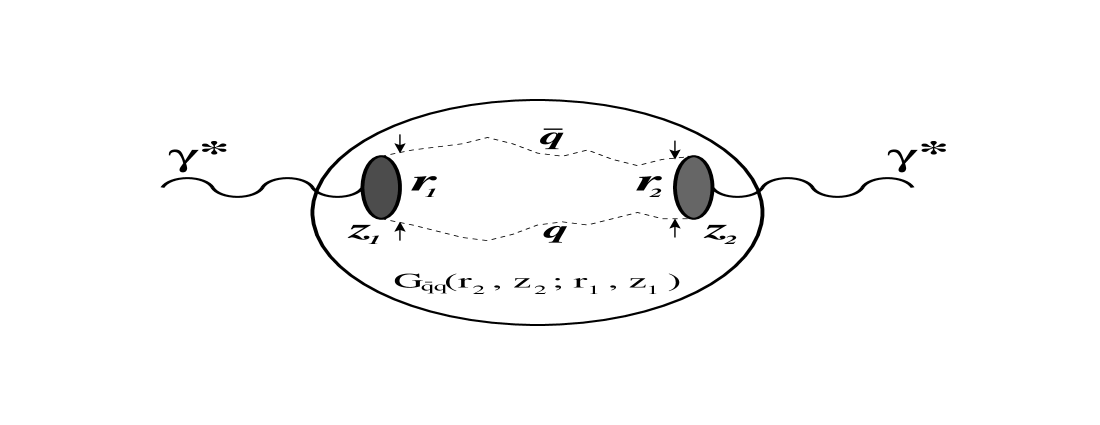
Figure 1: A cartoon for the shadowing term $\Delta\sigma$ in (2). Propagation of the $\bar{q}q$ pair through the nucleus is described by the Green function $G_{\bar{q}q}(\vec{r_{2}},z_{2};\vec{r_{1}},z_{1})$ which results from the summation over different paths of the $\bar{q}q$ pair.

The shadowing term in (2) is illustrated in Fig. 1. At the point $z_{1}$ the initial photon diffractively produces the $\bar{q}q$ pair ($\gamma^{*}N\to\bar{q}qN$) with transverse separation $\vec{r_{1}}$. The $\bar{q}q$ pair then propagates through the nucleus along arbitrary curved trajectories, which are summed over, and arrives at the point $z_{2}$ with a transverse separation $\vec{r_{2}}$. The initial and final separations are controlled by the LC wave function of the $\bar{q}q$ Fock component of the photon $\Psi_{\bar{q}q}(\vec{r},\alpha,Q^{2})$. During propagation through the nucleus the $\bar{q}q$ pair interacts with bound nucleons via dipole cross section $\sigma_{\bar{q}q}(r,s)$ which depends on the local transverse separation $\vec{r}$. The Green function $G_{\bar{q}q}(\vec{r_{2}},z_{2};\vec{r_{1}},z_{1})$ describes the propagation of the $\bar{q}q$ pair from $z_{1}$ to $z_{2}$.

The Green function $G_{\bar{q}q}(\vec{r_{2}},z_{2};\vec{r_{1}},z_{1})$ satisfies the time-dependent two-dimensional Schrödinger equation,

$$i\frac{d}{dz_{2}}\,G_{\bar{q}q}(\vec{r_{2}},z_{2};\vec{r_{1}},z_{1})=\left[\frac{\epsilon^{2}-\Delta_{r_{2}}}{2\,\nu\,\alpha\,(1-\alpha)}+V_{\bar{q}q}(z_{2},\vec{r}_{2},\alpha)\right]G_{\bar{q}q}(\vec{r_{2}},z_{2};\vec{r_{1}},z_{1})\ ,$$ (17)

with the boundary condition

$$G_{\bar{q}q}(\vec{r_{2}},z_{2};\vec{r_{1}},z_{1})|_{z_{2}=z_{1}}=\delta^{2}(\vec{r}_{1}-\vec{r}_{2})\,.$$ (18)

In Eq. (17) the Laplacian $\Delta_{r}$ acts on the coordinate $r$ and $\epsilon$ is given by (9).

The Green function $G_{\bar{q}q}(\vec{r_{2}},z_{2};\vec{r_{1}},z_{1})$ includes the phase shift between initial and final photons which is due to transverse and also longitudinal motion of the quarks. One can see the presence of the CL (1) in the kinetic term of the evolution Schrödinger equation (17), where the role of time is played by the longitudinal coordinate $z_{2}$. A part $\Delta_{r}/[2\nu\alpha(1-\alpha)]$ of this kinetic term takes care of the varying effective mass of the $\bar{q}q$ pair, $M_{\bar{q}q}^{2}=(m_{q}^{2}+k_{T}^{2})/\alpha(1-\alpha)$, and provides a proper phase shift. This is what the overall kinetic term consists when the transverse momentum squared of the quark is replaced by $k_{T}^{2}\rightarrow\Delta_{r}$. This dynamically varying effective mass controls CL defined by the Green function. The static part $Q^{2}+m_{q}^{2}/\alpha(1-\alpha)$ of the CL is connected with the longitudinal motion and is included in the Green function as well via the last phase shift factor (see Eq. (22) below). Consequently, the longitudinal momentum transfer is known and all the multiple interactions are included.

The imaginary part of the LC potential $V_{\bar{q}q}(z_{2},\vec{r}_{2},\alpha)$ in Eq. (17) is responsible for attenuation of the $\bar{q}q$ photon fluctuation in the medium, while the real part represents the interaction between the $q$ and $\bar{q}$. Because we are going to calculate the nuclear shadowing in DIS at medium and large $Q^{2}$ one can safely neglect this $\bar{q}$-$q$ interaction as was done also in [15].

In the LC Green function approach [15, 16, 17, 18] the physical photon $|\gamma^{*}\rangle$ is decomposed into different Fock states, namely, the bare photon $|\gamma^{*}\rangle_{0}$, $|\bar{q}q\rangle$, $|\bar{q}qG\rangle$, etc. As we mentioned above the higher Fock states containing gluons describe the energy dependence of the photoabsorption cross section on a nucleon. Besides, those Fock components lead also to GS as far as nuclear effects are concerned. However, these fluctuations are heavier and have a shorter coherence time (lifetime) than the lowest $|\bar{q}q\rangle$ state. Therefore, at medium energies only $|\bar{q}q\rangle$ fluctuations of the photon matter. Consequently, GS related to the higher Fock states will be dominated at high energies. Because we will calculate the nuclear shadowing at moderately small $x_{Bj}$ (medium values of $\nu$) we can neglect the GS for our purposes. This is supported also by the main goal of this paper which is based on comparison of the realistic calculations for nuclear shadowing with the results obtained within the harmonic oscillatory Green function approach and presented in the paper [15] where GS was neglected as well.

One can describe a propagation of a noninteracting $\bar{q}q$ pair in a nuclear medium by the Green function satisfying the evolution Eq. (17). The LC potential $V_{\bar{q}q}(z_{2},\vec{r},\alpha)$ in this case acquires only an imaginary part which represents absorption in the medium,

$$ImV_{\bar{q}q}(z_{2},\vec{r},\alpha)=-\frac{\sigma_{\bar{q}q}(\vec{r},s)}{2}\,\rho_{A}({b},z_{2})\,.$$ (19)

The analytical solution of Eq. (17) is known only for the harmonic oscillator potential $V(r)\propto r^{2}$. Consequently, one should use the dipole approximation

$$\sigma_{\bar{q}q}(r,s)=C(s)\,r^{2}\ ,$$ (20)

and uniform nuclear density

$$\rho_{A}(b,s)=\rho_{0}~{}\Theta(R_{A}^{2}-b^{2}-z^{2})\,,$$ (21)

in order to to obtain the Green function in an analytical form. In Eq. (21) $R_{A}$ is the nuclear radius. The solution in this case is the harmonic oscillator Green function [29],

$$G_{\bar{q}q}(\vec{r_{2}},z_{2};\vec{r_{1}},z_{1}) = \frac{b(\alpha)}{2\,\pi\,i\,{\rm sin}(\omega\,\Delta z)}\,{\rm exp}\left\{\frac{i\,b(\alpha)}{{\rm sin}(\omega\,\Delta z)}\,\Bigl{[}(r_{1}^{2}+r_{2}^{2})\,{\rm cos}(\omega\,\Delta z)-2\,\vec{r}_{1}\cdot\vec{r}_{2}\Bigr{]}\right\}$$

$$\times\, {\rm exp}\left[-\frac{i\,\epsilon^{2}\,\Delta z}{2\,\nu\,\alpha\,(1-\alpha)}\right]\ ,$$ (22)

where $\Delta z=z_{2}-z_{1}$ and

$$\omega=\frac{b(\alpha)}{\nu\;\alpha(1-\alpha)}\ ,$$ (23)

where

$$b^{2}(\alpha)=-i\,\rho_{A}({b},z)\,\nu\,\alpha\,(1-\alpha)\,C(s)\ .$$ (24)

The energy dependent factor $C(s)$ in Eq. (20) and the mean nuclear density $\rho_{0}$ in Eq. (21) can be adjusted by the procedure described in [16]. According this procedure the factor $C(s)$ is fixed by demanding that calculations employing the approximation Eq. (20) reproduce correctly the results based on the realistic cross section (given by KST parametrization Eq. (6) or by GBW model Eq. (5)) in the high-energy limit $l_{c}\gg R_{A}$ when the Green function takes the simple form (see Eq. (30) below). Consequently, the factor $C(s)$ is fixed by the relation,

$$\frac{\int d^{2}\,b\,\int d^{2}\,r\,\Bigl{|}\Psi_{\bar{q}q}^{T,L}(\vec{r},\alpha,Q^{2})\Bigr{|}^{2}\,\left\{1-\exp\,\Bigl{[}-\frac{1}{2}\,C(s)\,r^{2}\,T_{A}(b)\Bigr{]}\,\right\}}{\int d^{2}\,r\,\Bigl{|}\Psi_{\bar{q}q}^{T,L}(\vec{r},\alpha,Q^{2})\Bigr{|}^{2}\,C(s)\,r^{2}}$$

$$=\frac{\int d^{2}\,b\,\int d^{2}\,r\,\Bigl{|}\Psi_{\bar{q}q}^{T,L}(\vec{r},\alpha,Q^{2})\Bigr{|}^{2}\,\left\{1-\exp\,\Bigl{[}-\frac{1}{2}\,\sigma_{\bar{q}q}(r,s)\,T_{A}(b)\Bigr{]}\,\right\}}{\int d^{2}\,r\,\Bigl{|}\Psi_{\bar{q}q}^{T,L}(\vec{r},\alpha,Q^{2})\Bigr{|}^{2}\,\sigma_{\bar{q}q}(r,s)}\,,$$ (25)

where

$$T_{A}(b)=\int_{-\infty}^{\infty}\,dz\,\rho_{A}(b,z)\,$$ (26)

is the nuclear thickness calculated with the realistic Wood-Saxon form of the nuclear density with parameters taken from [30]. This procedure is performed separately for T and L polarized photons and for each value of $\alpha$. The value for the mean nuclear density $\rho_{0}$ in Eq. (21) is determined in a similar way using relation

$$\int\,d^{2}\,b\,\Biggl{[}1-exp\,\Biggl{(}-\sigma_{0}\,\rho_{0}\,\sqrt{R_{A}^{2}-b^{2}}\,\Biggr{)}\,\Biggr{]}=\int\,d^{2}\,b\,\Biggl{[}1-exp\,\Biggl{(}-\frac{1}{2}\,\sigma_{0}\,T_{A}(b)\,\Biggr{)}\,\Biggr{]}\,.$$ (27)

The value of $\rho_{0}$ turns out to be practically independent of the cross section $\sigma_{0}$ from 1 to 50 mb as was checked in [16, 25].

We would like to emphasize that only in the high energy limit, $l_{c}\gg R_{A}$, it is possible to resum the whole multiple scattering series in an eikonal-formula. Correspondingly, the transverse separation $r$ between $\bar{q}$ and $q$ does not vary during propagation through the nucleus (Lorentz time dilation). Then the total photoabsorption cross section on a nucleus reads [21]

$$\sigma^{\gamma^{*}A}(s,Q^{2}) = 2\,\int d^{2}b\,\int d^{2}r\,\int_{0}^{1}d\alpha\,|\Psi_{\bar{q}q}(\vec{r},\alpha,Q^{2})|^{2}\,\left\{1-\exp\,\Bigl{[}-\frac{1}{2}\,\sigma_{\bar{q}q}(r,s)\,T_{A}(b)\Bigr{]}\,\right\}$$ (28)

$$\equiv 2\,\int d^{2}b\,\left\{1-\Biggl{\langle}\,\exp\,\Bigl{[}-\frac{1}{2}\,\sigma_{\bar{q}q}(r,s)\,T_{A}(b)\Bigr{]}\,\Biggr{\rangle}\,\right\}\,.$$

Note that the averaging of the whole exponential in (28) makes this expression different from the Glauber eikonal approximation where $\sigma(r,s)$ is averaged in the exponent,

$$\sigma^{\gamma^{*}A}_{Glauber}(s,Q^{2})=2\,\int d^{2}b\,\left\{1-\,\exp\,\Bigl{[}-\frac{1}{2}\,\sigma^{\gamma^{*}N}(s,Q^{2})\,T_{A}(b)\Bigr{]}\,\right\}\,.$$ (29)

The difference is known as Gribov’s inelastic corrections [31]. In the case of DIS the Glauber approximation does not make sense (because of a small value of $\sigma^{\gamma^{*}p}$, which is at most of the order of $100\,\mu b$ for real photons) and the whole cross section is due to the inelastic shadowing.

The eikonal formula (28) for the total photoabsorption cross section on a nucleus can be obtained as a limiting case of the Green function formalism. Indeed, in the high energy limit, $\nu\rightarrow\infty$ the kinetic term in Eq. (17) can be neglected and the Green function reads

$$G_{\bar{q}q}(\vec{r_{2}},z_{2};\vec{r_{1}},z_{1})|_{\nu\to\infty}=\delta(\vec{r_{2}}-\vec{r_{1}})\,\exp\Biggl{[}-\frac{1}{2}\,\sigma_{\bar{q}q}(r_{2},s)\,\int_{z_{1}}^{z_{2}}\,dz\,\rho_{A}(b,z)\Biggr{]}\,.$$ (30)

After substitution of this expression into Eqs. (2), (15) and (16) one arrives at the result (28).

For smaller energies when $l_{c}\sim R_{A}$, one has to take into account the variation of the transverse size $r$ during propagation of the $\bar{q}q$ pair through the nucleus. This transverse size variation is naturally included using correct quantum-mechanical treatment based on the Green function formalism presented above.

The overall total photoabsorption cross section on a nucleus is given as a sum of T and L polarizations, $\sigma^{\gamma^{*}A}=\sigma_{T}^{\gamma^{*}A}+\epsilon^{\prime}\,\sigma_{L}^{\gamma^{*}A}$, assuming that the photon polarization $\epsilon^{\prime}=1$. If one takes into account only $\bar{q}q$ Fock component of the photon the full expression after summation over all flavors, colors, helicities and spin states has the following form [32]

$$\sigma^{\gamma^{*}A}(x_{Bj},Q^{2}) = A\,\sigma^{\gamma^{*}N}(x_{Bj},Q^{2})-\Delta\,\sigma(x_{Bj},Q^{2})$$

$$= A\,\int\,d^{2}r\,\int_{0}^{1}\,d\alpha\,\sigma_{\bar{q}q}(r,s)\,\Biggl{(}\Bigl{|}\Psi^{T}_{\bar{q}q}(\vec{r},\alpha,Q^{2})\Bigr{|}^{2}+\Bigl{|}\Psi^{L}_{\bar{q}q}(\vec{r},\alpha,Q^{2})\Bigr{|}^{2}\Biggr{)}$$

$$- \frac{3\,\alpha_{em}}{(2\pi)^{2}}\,\sum_{f=1}^{N_{f}}\,Z_{f}^{2}\,Re\,\int\,d^{2}b\,\int_{-\infty}^{\infty}\,dz_{1}\,\int_{z_{1}}^{\infty}\,dz_{2}\,\int_{0}^{1}\,d\alpha\,\int\,d^{2}r_{1}\,\int\,d^{2}r_{2}$$

$$\times\,\rho_{A}(b,z_{1})\,\rho_{A}(b,z_{2})\,\sigma_{\bar{q}q}(r_{2},s)\,\sigma_{\bar{q}q}(r_{1},s)$$

$$\times\,\Biggl{\{}\Bigl{[}\,\alpha^{2}+(1-\alpha)^{2}\,\Bigr{]}\,\epsilon^{2}\,\frac{\vec{r_{1}}\,\cdot\,\vec{r_{2}}}{r_{1}\,r_{2}}\,K_{1}(\epsilon\,r_{1})\,K_{1}(\epsilon\,r_{2})$$

$$\,\,\,\,\,\,\,\,\,\,\,\,\,\,\,+\,\Bigl{[}\,m_{f}^{2}+4\,Q^{2}\,\alpha^{2}\,(1-\alpha)^{2}\,\Bigr{]}\,K_{0}(\epsilon\,r_{1})\,K_{0}(\epsilon\,r_{2})\Biggr{\}}\,G_{\bar{q}q}(\vec{r_{2}},z_{2};\vec{r_{1}},z_{1})\,.$$

Here $\Bigl{|}\,\Psi^{T,L}_{\bar{q}q}(\vec{r},\alpha,Q^{2})\,\Bigr{|}^{2}$ are the absolute squares of the LC wave functions for the $\bar{q}q$ fluctuation of T and L polarized photons summed over all flavors with the form given by Eqs. (12) and (13), respectively.

In the high energy limit after substitution of expression (30) for the Green function into Eq. (2) one arrives at the following results, which corresponds to Eq. (28) after inclusion of a sum of T and L polarizations :

$$\sigma^{\gamma^{*}A}(x_{Bj},Q^{2}) = 2\,\int\,d^{2}b\,\int\,d^{2}r\,\int_{0}^{1}\,d\alpha\left\{1-\exp\,\Bigl{[}-\frac{1}{2}\,\sigma_{\bar{q}q}(r,s)\,T_{A}(b)\Bigr{]}\,\right\}$$

$$\times\,\frac{2\,N_{C}\,\alpha_{em}}{(2\pi)^{2}}\,\sum_{f=1}^{N_{f}}\,Z_{f}^{2}\,\Biggl{\{}\Bigl{[}\,\alpha^{2}+(1-\alpha)^{2}\,\Bigr{]}\,\epsilon^{2}\,K_{1}^{2}(\epsilon\,r)\,$$

$$\,\qquad\qquad\qquad\qquad+\,\Bigl{[}\,m_{f}^{2}+4\,Q^{2}\,\alpha^{2}\,(1-\alpha)^{2}\,\Bigr{]}\,K_{0}^{2}(\epsilon\,r)\,\Biggr{\}}\,.$$

At photon polarization parameter $\epsilon^{\prime}=1$ the structure function ratio $F_{2}^{A}(x_{Bj},Q^{2})/F_{2}^{N}(x_{Bj},Q^{2})$ can be expressed via ratio of the total photoabsorption cross sections

$$\frac{F_{2}^{A}(x_{Bj},Q^{2})}{F_{2}^{N}(x_{Bj},Q^{2})}=\frac{\sigma_{T}^{\gamma^{*}A}(x_{Bj},Q^{2})+\sigma_{L}^{\gamma^{*}A}(x_{Bj},Q^{2})}{\sigma_{T}^{\gamma^{*}N}(x_{Bj},Q^{2})+\sigma_{L}^{\gamma^{*}N}(x_{Bj},Q^{2})}\,,$$ (33)

where the numerator on right-hand side (r.h.s.) is given by Eq. (2), whereas denominator can be expressed as the first term of Eq. (2) divided by the mass number $A$.

Finally we would like to emphasize that $\bar{q}q$ Fock component of the photon represents the higher twist shadowing correction [16]. This correction vanishes at large quark masses as $1/m_{f}^{2}$. Not so for the higher Fock states containing gluons and leading to GS. GS represents the leading twist shadowing correction [19, 33]. Besides, a steep energy dependence of the dipole cross section $\sigma_{\bar{q}q}(r,s)$ (see Eqs. (5) and (6)) especially at smaller dipole sizes $r$ causes a steep energy rise of both corrections.

3 Algorithm for numerical solution of the evolution equation for the Green function

As we mentioned in the previous section, an explicit analytical expression for the Green function $G_{\bar{q}q}(\vec{r_{2}},z_{2};\vec{r_{1}},z_{1})$ (22) can be found only for the quadratic form (20) of the dipole cross section and for uniform nuclear density function (21). It was already analyzed in [15, 16] that such an approximation should have a reasonable accuracy, especially for heavy nuclei. We also discussed in the previous Section that the higher accuracy can be achieved taking into account the fact that the expression (28) in the high energy limit can be easily calculated using realistic parametrizations of the dipole cross section (see Eqs. (5) and (6)) and a realistic nuclear density function $\rho_{A}(b,z)$ [30]. Consequently, one needs to know the full Green function only in the transition region from non-shadowing ($x_{Bj}\sim 0.1$) to a fully developed shadowing given by Eq. (28). Therefore the value of the energy dependent factor $C(s)$ in Eq. (20) was fixed [15, 16] separately for T and L photon polarizations (see Eq. (25)) in a such way that the asymptotic nuclear shadowing in DIS is the same for the realistic parametrizations of the dipole cross section Eqs. (5) and (6) and for approximation (20). Correspondingly, the value $\rho_{0}$ of the uniform nuclear density (21) was fixed in an analogical way as given by Eq. (27) and described shortly in the previous Section. Such a procedure for determination of the factor $C(s)$ and $\rho_{0}$ was applied also in [17, 18] with respect to incoherent and coherent production of vector mesons off nuclei.

In order to remove the above mentioned uncertainties one should solve the evolution equation for the Green function numerically for arbitrary parametrization of the dipole cross section and for realistic nuclear density function. However, the tax for this general solution is that one does not obtain a nice analytical form for the Green function. First we present an algorithm for the exact numerical solution of the evolution equation. Using this algorithm we will calculate the nuclear shadowing in DIS and study how the new results change in comparison with predictions [15] based on above mentioned approximations leading to harmonic oscillator Green function (22).

In the process of numerical solution of the Schrödinger equation (17) for the Green function $G_{\bar{q}q}(\vec{r_{2}},z_{2};\vec{r_{1}},z_{1})$ it is not very convenient to treat the initial condition (18) with two-dimensional Delta function on the r.h.s. In order to remove this problem one should use the following substitutions

$$g_{1}(\vec{r_{2}},z_{2};z_{1})=\int\,d^{2}r_{1}\,K_{0}(\epsilon\,r_{1})\,\sigma_{\bar{q}q}(r_{1},s)\,G_{\bar{q}q}(\vec{r_{2}},z_{2};\vec{r_{1}},z_{1})\,,$$ (34)

and

$$\frac{\vec{r_{2}}}{r_{2}}\,g_{2}(\vec{r_{2}},z_{2};z_{1})=\int\,d^{2}r_{1}\,K_{1}(\epsilon\,r_{1})\,\sigma_{\bar{q}q}(r_{1},s)\,\frac{\vec{r_{1}}}{r_{1}}\,G_{\bar{q}q}(\vec{r_{2}},z_{2};\vec{r_{1}},z_{1})\,.$$ (35)

Consequently, after some algebra with Eq. (17) one can introduce new functions $g_{1}(\vec{r_{2}},z_{2};z_{1})$ and $g_{2}(\vec{r_{2}},z_{2};z_{1})$ which satisfy now the following evolution equations

$$i\frac{d}{dz_{2}}\,g_{1}(\vec{r_{2}},z_{2};z_{1})=\left\{\frac{1}{2\,\mu_{\bar{q}q}}\left[\epsilon^{2}-\frac{\partial^{2}}{\partial\,r_{2}^{2}}-\frac{1}{r_{2}}\,\frac{\partial}{\partial\,r_{2}}\right]+V_{\bar{q}q}(z_{2},\vec{r}_{2},\alpha)\right\}g_{1}(\vec{r_{2}},z_{2};z_{1})\$$ (36)

and

$$i\frac{d}{dz_{2}}\,g_{2}(\vec{r_{2}},z_{2};z_{1})=\left\{\frac{1}{2\,\mu_{\bar{q}q}}\left[\epsilon^{2}-\frac{\partial^{2}}{\partial\,r_{2}^{2}}-\frac{1}{r_{2}}\,\frac{\partial}{\partial\,r_{2}}+\frac{1}{r_{2}^{2}}\right]+V_{\bar{q}q}(z_{2},\vec{r}_{2},\alpha)\right\}g_{2}(\vec{r_{2}},z_{2};z_{1})\ ,$$ (37)

with the boundary conditions

$$g_{1}(\vec{r_{2}},z_{2};z_{1})|_{z_{2}=z_{1}}=K_{0}(\epsilon\,r_{2})\,\sigma_{\bar{q}q}(r_{2},s)$$ (38)

and

$$g_{2}(\vec{r_{2}},z_{2};z_{1})|_{z_{2}=z_{1}}=K_{1}(\epsilon\,r_{2})\,\sigma_{\bar{q}q}(r_{2},s)\,.$$ (39)

In Eqs. (36) and (37) the quantity

$$\mu_{\bar{q}q}=\nu\,\alpha\,(1-\alpha)$$ (40)

plays the role of the reduced mass of the $\bar{q}q$ pair. Consequently, the expression (2) for total photoabsorption cross section on a nucleus now reads

$$\sigma^{\gamma^{*}A}(x_{Bj},Q^{2}) = A\,\sigma^{\gamma^{*}N}(x_{Bj},Q^{2})-\Delta\,\sigma(x_{Bj},Q^{2})$$

$$= A\,\int\,d^{2}r\,\int_{0}^{1}\,d\alpha\,\sigma_{\bar{q}q}(r,s)\,\Biggl{(}\Bigl{|}\Psi^{T}_{\bar{q}q}(\vec{r},\alpha,Q^{2})\Bigr{|}^{2}+\Bigl{|}\Psi^{L}_{\bar{q}q}(\vec{r},\alpha,Q^{2})\Bigr{|}^{2}\Biggr{)}$$

$$- \frac{3\,\alpha_{em}}{(2\pi)^{2}}\,\sum_{f=1}^{N_{f}}\,Z_{f}^{2}\,Re\,\int\,d^{2}b\,\int_{-\infty}^{\infty}\,dz_{1}\,\int_{z_{1}}^{\infty}\,dz_{2}\,\int_{0}^{1}\,d\alpha\,\int\,d^{2}r_{2}$$

$$\times\,\rho_{A}(b,z_{1})\,\rho_{A}(b,z_{2})\,\sigma_{\bar{q}q}(r_{2},s)\,$$

$$\times\,\Biggl{\{}\Bigl{[}\,\alpha^{2}+(1-\alpha)^{2}\,\Bigr{]}\,\epsilon^{2}\,K_{1}(\epsilon\,r_{2})\,g_{2}(\vec{r_{2}},z_{2};z_{1})$$

$$\,\,\,\,\,\,\,\,\,\,\,\,\,\,\,+\,\Bigl{[}\,m_{f}^{2}+4\,Q^{2}\,\alpha^{2}\,(1-\alpha)^{2}\,\Bigr{]}\,K_{0}(\epsilon\,r_{2})\,g_{1}(\vec{r_{2}},z_{2};z_{1})\Biggr{\}}\,.$$

There are several approaches for solving the time-dependent one-dimensional Schrödinger equation (see for example [34, 35, 36, 37]). One can not adopt directly these approaches for our purposes because one needs to treat the time-dependent two-dimensional Schrödinger equation (see Eq. (17)). Therefore, we will consider a modification of the method based on the Crank-Nicholson algorithm [38]. Details of this method for numerical solution of Eqs. (36) and (37) are presented in the Appendix A.

4 Numerical results

As we mentioned above the main goal of this paper is to present for the first time the realistic predictions for nuclear shadowing based on exact numerical solutions of the evolution equation for the Green function. These predictions will be confronted with approximate results obtained using harmonic oscillatory form of the Green function (22). The proposed algorithm (see Appendix A) for numerical solution of the evolution equation for the Green function gives a possibility to calculate nuclear shadowing for arbitrary LC potential $V_{\bar{q}q}(z,\vec{r},\alpha)$ and nuclear density function. It allows to perform an independent cross-check whether the results calculated using quadratic form of the imaginary part, $Im\,V_{\bar{q}q}(z,\vec{r},\alpha)=-1/2\,\rho_{A}(b,z)\,C\,r^{2}$ ($C\approx 3$), of the LC potential and uniform density function $\rho_{A}(b,z)=\rho_{0}=0.16\,\mbox{fm}^{-3}$ correspond to predictions for nuclear shadowing taken from [15] calculated using Green function of the form (22). Therefore, we calculate nuclear shadowing for calcium and lead as was done in [15].

In order to realize one-to-one comparison with the results from the paper [15] we made a several assumptions. As was mentioned in Section (2) we neglect the real part of the LC potential $V_{\bar{q}q}(z_{2},\vec{r_{2}},\alpha)$ in the Schrödinger equation (17) analyzing DIS at medium and large values of $Q^{2}$. We neglect also the effects of nuclear antishadowing assuming that they are beyond the shadowing dynamics. The corresponding values of Bjorken $x_{Bj}$ cover medium and medium large values, $x_{Bj}\in(0.001,0.1)$. For this reason we omit the effects of GS which are important at small $x_{Bj}$ (large $\nu$). Although gluons can give some small (not negligible) contribution to nuclear shadowing at lower limit ($x_{Bj}\sim 0.001$) of investigated interval of $x_{Bj}$, for simplicity we do not include them in calculations as was done also in the paper [15].

We use an algorithm for numerical solution of the Schrödinger equation for the Green function described in Section (3) and Appendix A. Numerical solution of Schrödinger equation allows us to use realistic nuclear density function and realistic parametrizations of the dipole cross section, $\sigma_{\bar{q}q}(r,s)$. These parametrizations naturally incorporate the energy ($x_{Bj}-$ ) dependence of $\sigma_{\bar{q}q}(r,s)$ which was not included so far in calculations (see [15]). We took the nuclear density function in Woods-Saxon form [30]. The realistic calculations of nuclear shadowing were performed at two different parametrizations of the dipole cross section, GBW [24] given by Eq. (5) and KST [19] given by Eq. (6).

Nuclear shadowing effects were studied via $x_{Bj}$- behavior of the ratio of proton structure functions (33) divided by the mass number $A$. The proton structure functions $F_{2}^{N}(x_{Bj},Q^{2})$ and $F_{2}^{A}(x_{Bj},Q^{2})$ were calculated perturbatively (we fixed the quark masses at $m_{q}=0.3\,\mbox{GeV}$, $m_{s}=0.45\,\mbox{GeV}$ and $m_{c}=1.5\,\mbox{GeV}$) via total photoabsorption cross sections $\sigma^{\gamma^{*}N}(x_{Bj},Q^{2})$ and $\sigma^{\gamma^{*}A}(x_{Bj},Q^{2})$ given by Eqs. (4) and (3), respectively. The results of calculations are shown in Fig. 2. The dashed curves represent the predictions based on the harmonic oscillator Green function (22) approach corresponding to a constant nuclear density function $\rho_{0}=0.16\,fm^{-3}$ and quadratic form of the dipole cross section (20) with a constant factor $C(s)\approx 3$. The dotted curves correspond to calculations using the same quadratic form of the dipole cross section but realistic nuclear density function of the Woods-Saxon form [30]. The thin and thick solid curve corresponds to realistic calculations based on the exact numerical solution of the evolution equation (17) for the Green function using GBW (5) and KST (6) parametrization of the dipole cross section, respectively.

Figure 2: Nuclear shadowing for calcium and lead. The dashed curves are calculated using harmonic oscillator Green function approach (22) corresponding to constant nuclear density (21) and dipole cross section (20) with $C(s)\approx 3$ [15]. The dotted curves are calculated for the same quadratic form of the dipole cross section but for realistic nuclear density function of the Woods-Saxon form [30]. The thin and thick solid curves correspond to exact numerical solution of the evolution equation for the Green function using GBW [24] and KST [19] parametrization of the dipole cross section, respectively.

At low $x_{Bj}\mathrel{\hbox to0.0pt{\lower 4.0pt\hbox{\hskip 1.0pt$\sim$}\hss}\raise 1.0pt\hbox{$<$}}0.001$ one should expect a saturation of nuclear shadowing at level given by Eqs. (28) or (2). For parametrization (20) of the dipole cross section with constant $C(s)\approx 3$ [15], this saturation level is fixed at some value depending on $Q^{2}$ and the nuclear mass number $A$ (see the dashed and dotted lines in Fig. 2). However, it is not so for realistic parametrizations Eq. (5) and (6) where the saturation level is not fixed exactly due to energy (Bjorken $x_{Bj}$-) dependence of the dipole cross section $\sigma_{\bar{q}q}(r,s)$.

In the process of realistic calculations of nuclear shadowing (3) we tested the correctness of tremendous computations based on the numerical evaluations of the functions $g_{1}$ and $g_{2}$ from differential equations (36) and (37) in a such way that in the high energy limit the results for nuclear shadowing must be the same as obtained from the expression (2).

Results presented in Fig. 2 show quite a large deviation of the predictions within harmonic oscillator Green function approach (dashed lines) from realistic calculations performed for both parametrizations of the dipole cross section (thin and thick solid lines). This deviation depends on $Q^{2}$ and the nuclear mass number $A$ as a result of quadratic form of the dipole cross section (see Eq. (20) with $C(s)\approx 3$) and application of the constant nuclear density function, $\rho_{0}=0.16\,\mbox{fm}^{-3}$. There is even not negligible difference between predictions using constant and realistic form of the nuclear density function (compare dashed and dotted lines). It allows to make conclusion that the form of nuclear density function is also important for model predictions. Note, that the dashed curves correspond to predictions presented in the paper [15]. It is another cross-check for correctness of calculations using above presented algorithm for numerical solution of the evolution equation for the Green function.

As one can see from Fig. 2 at small and medium values of $Q^{2}$ ($Q^{2}=2$ and $6\,\mbox{GeV}^{2}$), the approximate calculations depicted by the dashed lines agree better with realistic calculations using KST parametrization [19] of the dipole cross section expressed by Eq. (6). At large $Q^{2}=18\,\mbox{GeV}^{2}$ and at $x_{Bj}\mathrel{\hbox to0.0pt{\lower 4.0pt\hbox{\hskip 1.0pt$\sim$}\hss}\raise 1.0pt\hbox{$<$}}0.005$, however, the dashed lines seem to be in better agreement with realistic calculations using GBW parametrization [24] given by Eq. (5). This fact confirms discussion presented in Section 2 that the GBW model is suited better at medium and large $Q^{2}\mathrel{\hbox to0.0pt{\lower 4.0pt\hbox{\hskip 1.0pt$\sim$}\hss}\raise 1.0pt\hbox{$>$}}5\div 10\,\mbox{GeV}^{2}$ and at medium small and small $x_{Bj}\mathrel{\hbox to0.0pt{\lower 4.0pt\hbox{\hskip 1.0pt$\sim$}\hss}\raise 1.0pt\hbox{$<$}}0.01$ whereas the KST model prefers low and medium values of $Q^{2}\mathrel{\hbox to0.0pt{\lower 4.0pt\hbox{\hskip 1.0pt$\sim$}\hss}\raise 1.0pt\hbox{$<$}}10\,\mbox{GeV}^{2}$.

Nevertheless, calculations of nuclear shadowing using harmonic oscillator Green function can be improved by determination of the energy-dependent factor $C(s)$ in approximation (20) by the procedure mentioned shortly above in Sect. 2 and described in details in [16, 25] for calculation of nuclear shadowing in DIS and in [17, 18] for calculation of nuclear transparency for coherent and incoherent vector meson production off nuclei. That procedure allows to evaluate the factor $C(s)$ for each c.m. energy squared $s$ depending on the values of $Q^{2}$ and $A$. As a result, at fixed $Q^{2}$ the parameter $C(s)$ rises with $s$ as a consequence of energy- ($x_{Bj}$- ) dependent realistic dipole cross section given by Eqs. (5) and (6). Thus, the value of $C(s)$ at $s$ corresponding to $x_{Bj}\in(0.001,0.01)$ exceeds so the fixed value $C(s)\approx 3$ used in predictions in [15]. This fact should lead to a larger nuclear shadowing at $x_{Bj}\in(0.001,0.01)$ in comparison with what is shown in Fig. 2 by the dashed lines.

As we mentioned above in Section 2 the difference between the thin and thick solid lines in Fig. 2 can be treated as a measure of the theoretical uncertainty in the kinematic region where the both realistic parametrizations GBW (5) and KST (6) are applicable. Therefore, it would be very useful for the future realistic calculations to connect advantages of both parametrizations in the modified model for dipole cross section which can be then safely used for all dipole sizes covering perturbative as well as nonperturbative region.

5 Summary and conclusions

We present a rigorous quantum-mechanical approach based on the light-cone QCD Green function formalism which naturally incorporates the interference effects of CT and CL. Within this approach [15, 20, 16] we study nuclear shadowing in deep-inelastic scattering at moderately small Bjorken $x_{Bj}$.

Calculations of nuclear shadowing performed so far were based only on the efforts to solve the evolution equation for the Green function analytically. Analytical harmonic oscillatory form of the Green function (22) could be obtained only taking into account additional approximations like a constant nuclear density function (21) and the dipole cross section of the quadratic form (20). It brings additional theoretical uncertainties in predictions for nuclear shadowing. In order to remove these uncertainties we solve the evolution equation for the Green function numerically.

We perform for the first time the exact numerical solution of the evolution equation for the Green function using two realistic parametrizations of the dipole cross section (GBW [24] and KST [19]) and realistic nuclear density function of the Woods-Saxon form [30]. This exact numerical solution does not require to put any additional approximations. Analyzing only medium and large values of $Q^{2}$ we neglect the real part of the LC potential $V_{\bar{q}q}(z_{2},\vec{r_{2}},\alpha)$ in the time-dependent two-dimensional Schrödinger equation (17) responsible for interaction between $\bar{q}$ and $q$. We neglect also the nuclear antishadowing effect as was done in [15] assuming that it is beyond the shadowing dynamics. Performing calculations at medium and medium large values of $x_{Bj}\in(0.001,0.1)$ we neglect for simplicity also the contribution of the higher Fock states leading to effects of GS. This is supported also by the one-to-one comparison of the realistic calculations with the predictions from the paper [15], where GS is neglected as well.

In order to compare the realistic calculations with data on nuclear shadowing, the effects of GS should be taken into account especially at $x_{Bj}\mathrel{\hbox to0.0pt{\lower 4.0pt\hbox{\hskip 1.0pt$\sim$}\hss}\raise 1.0pt\hbox{$<$}}0.001$. The same path integral technique [19] can be applied in this case. However, the calculations of GS (see [39], for example) were performed so far using analogical approximations as already mentioned above like a constant nuclear density function and the quadratic form (see Eq. (20)) of the dipole gluon-gluon-nucleon cross section, $\sigma_{gg}(r,s)=9/4\,\sigma_{\bar{q}q}(r,s)$ plus further assumptions which simplify the final expression for GS. Moreover, the GS was calculated from the shadowing of the $|\bar{q}qG\rangle$ Fock component of a longitudinally polarized photon at sufficiently large $Q^{2}$ where the three-body Green function, $G_{\bar{q}qG}$, is assumed to be factorized as a product of two-body ones [19]. Using the algorithm presented above one can calculate GS exactly for the general case of nuclear shadowing for a three-parton system, i.e. one can solve numerically the Schrödinger equation for the Green function $G_{\bar{q}qG}$ describing propagation of the $\bar{q}qG$ system through a nuclear medium. We are going to calculate numerically the gluon contribution to nuclear shadowing in a forthcoming paper.

We present analogical numerical results of nuclear shadowing in DIS with correct quantum-mechanical treatment of multiple interaction of the virtual photon fluctuations and of the nuclear form factor as was done in [15, 16]. We found quite large differences (see Fig. 2) between realistic predictions and the approximate results obtained within harmonic oscillator Green function approach (22). At small and medium values of $Q^{2}$ the approximate predictions agree better with realistic calculations using KST parametrization [19] of the dipole cross section Eq. (6). At large $Q^{2}$, however, they seem to be in better agreement with realistic calculations using GBW parametrization [24] given by Eq. (5). It confirms the fact that the GBW model is well suited at medium and large $Q^{2}$ and at medium small and small $x_{Bj}$, whereas the KST model prefers low and medium values of $Q^{2}$. Therefore, the future realistic calculations require to revise existing parametrizations for dipole cross section in order to be used for whole region of dipole sizes.

Concluding, the universality of the LC dipole approach based on the Green function formalism allows us to apply the presented algorithm for the exact numerical solution of the evolution equation for the Green function also for calculations of other processes like Drell-Yan production, vector meson production etc. including the effects of gluon shadowing at high energies as well.

Acknowledgments: We are grateful to Alexander Tarasov for stimulating discussions. This work has been supported in part by the Slovak Funding Agency, Grant No. 2/2099/22 and Grant No. 2/1169/21.

Appendix A Description of the method for numerical solution of the time-dependent Schrödinger equation

We treat here only differential equation (36) for the function $g_{1}(\vec{r_{2}},z_{2};z_{1})$ and describe in details the method for its numerical solution. This method is then analogically applicable for numerical solution of Eq. (37) for the function $g_{2}(\vec{r_{2}},z_{2};z_{1})$.

Looking at Eq. (36), one needs to solve numerically the following time-dependent Schrödinger equation

$$i\,\frac{d}{dt}\,g_{1}(\vec{r},t)=\hat{H}\,g_{1}(\vec{r},t)\,,$$ (A.1)

where $\hat{H}$ is the Hamiltonian operator defined by

$$\hat{H}=\frac{1}{2\,\mu_{\bar{q}q}}\,\Biggl{[}\epsilon^{2}-\frac{\partial^{2}}{\partial r^{2}}-\frac{1}{r}\,\frac{\partial}{\partial r}\,\Biggr{]}+V_{\bar{q}q}(r,t)\,.$$ (A.2)

Here the complex LC potential $V_{\bar{q}q}(r,t)$ is assumed to have only the imaginary part responsible for absorption of $\bar{q}q$ photon fluctuation in the nuclear medium (see discussion in Section 2 and Eq. (19)),

$$V_{\bar{q}q}(r,t)=-\frac{i}{2}\,\sigma_{\bar{q}q}(r,s)\,\rho_{A}(b,t)\,,$$ (A.3)

where $b$ is the nuclear impact parameter and $r$ is the transverse separation between $\bar{q}$ and $q$ at the point $z_{2}$. The longitudinal coordinate $z_{2}$ plays the role of time $t$ for the $\bar{q}q$ pair propagation from the point $z_{1}$. In Eq. (A.2) the quantity $\mu_{\bar{q}q}$ is expressed by Eq. (40).

Ignoring for a moment the fact that $\hat{H}$ is an operator, Eq. (A.1) has the formal solution,

$$g_{1}(\vec{r},t)=exp\,(-i\,t\,\hat{H})\,g_{1}(\vec{r},0)\,,$$ (A.4)

where $g_{1}(\vec{r},0)$ is the function at $t=0$. Thus, if one knows $g_{1}(\vec{r},0)$, one can formally calculate the behavior at all future times using Eq. (A.4). Unfortunately, this formal solution is not of much practical use since the Taylor expansion of the exponential factor in Eq. (A.4) involves a very large (infinite) number of terms. However, it does suggest a way to proceed numerically. Let us consider a formal solution applying over a very small time interval. After time discretization in steps $\Delta t$ using Eq. (A.4) we obtain

$$g_{1}(\vec{r},t+\Delta t)=exp\,(-i\,\Delta t\,\hat{H})\,g_{1}(\vec{r},t)\,.$$ (A.5)

Consequently, at sufficiently small time intervals $\Delta t$ the higher order terms in Taylor expansion of the exponential factor in (A.4) are small enough and can be neglected. Then we can include only the term linear in $\hat{H}$,

$$exp\,(-i\,\Delta t\,\hat{H})\approx 1-i\,\Delta t\,\hat{H}\,.$$ (A.6)

However, this way of approximating the exponential factor is not correct with regard to maintaining unitarity [38]. In order to settle this problem one should use an approach that satisfy unitarity writing the exponential factor in Eq. (A.5) in what is known as the Cayley form

$$exp\,(-i\,\Delta t\,\hat{H})\approx\frac{1-\frac{1}{2}\,i\,\Delta t\,\hat{H}}{1+\frac{1}{2}\,i\,\Delta t\,\hat{H}}\,.$$ (A.7)

Using this approximation and Eq. (A.4) to propagate the function $g_{1}(\vec{r},t)$ forward in time we obtain

$$g_{1}(\vec{r},t+\Delta t)\approx\frac{1-\frac{1}{2}\,i\,\Delta t\,\hat{H}}{1+\frac{1}{2}\,i\,\Delta t\,\hat{H}}\,g_{1}(\vec{r},t)\,.$$ (A.8)

This expression will be the basis for numerical approach. From (A.8) we first obtain

$$\Biggl{[}1+\frac{1}{2}\,i\,\Delta t\,\hat{H}\,\Biggr{]}\,g_{1}(\vec{r},t+\Delta t)=\Biggl{[}1-\frac{1}{2}\,i\,\Delta t\,\hat{H}\,\Biggr{]}\,g_{1}(\vec{r},t)\,.$$ (A.9)

Given (A.9), a natural way to proceed is to discretize also space into units of size $\Delta r$ and write the function $g_{1}$ as $g_{1}(r,t)\equiv g_{1}(m\,\Delta r,n\,\Delta t)$. Then one can express the first and second derivatives included in the Hamiltonian operator (A.2) in the usual finite-difference form :

$$\frac{\partial}{\partial\,r}\,g_{1}(r,t)\approx\frac{g_{1}(r+\Delta r)-g_{1}(r,t)}{\Delta r}=\frac{g_{1}(m+1,n)-g_{1}(m,n)}{\Delta r}$$ (A.10)

and

$$\frac{\partial^{2}}{\partial\,r^{2}}\,g_{1}(r,t) \approx \frac{\partial}{\partial\,r}\,\Biggl{[}\frac{g_{1}(r+\Delta r)-g_{1}(r,t)}{\Delta r}\,\Biggr{]}=\frac{g_{1}(r+\Delta r,t)-2\,g_{1}(r,t)+g_{1}(r-\Delta r,t)}{(\Delta r)^{2}}$$ (A.11)

$$= \frac{g_{1}(m+1,n)-2\,g_{1}(m,n)+g_{1}(m-1,n)}{(\Delta r)^{2}}$$

If one replaces in Eq. (A.9) the Hamiltonian operator by (A.2), converting everything to finite-deference form using also Eqs. (A.10) and (A.11), and rearranging a few terms one obtains the following expression

$$g_{1}(m+1,n+1) + h(m)\,\Biggl{[}\,2\,i\,\lambda-2\,\mu_{\bar{q}q}\,(\Delta r)^{2}\,V(m,n+1)-\epsilon^{2}\,(\Delta r)^{2}-2-\frac{1}{m}\,\Biggr{]}\,g_{1}(m,n+1)$$

$$+ h(m)\,g_{1}(m-1,n+1)$$

$$=-g_{1}(m+1,n) + h(m)\,\Biggl{[}\,2\,i\,\lambda+2\,\mu_{\bar{q}q}\,(\Delta r)^{2}\,V(m,n)+\epsilon^{2}\,(\Delta r)^{2}+2+\frac{1}{m}\,\Biggr{]}\,g_{1}(m,n)$$ (A.12)

$$- h(m)\,g_{1}(m-1,n)\,,$$

where the function $h(m)$ is given by

$$h(m)=\frac{m}{1+m}$$ (A.13)

and

$$\lambda=\frac{2\,(\Delta r)^{2}\,\mu_{\bar{q}q}}{\Delta t}$$ (A.14)

with the reduced mass of $\bar{q}q$ pair defined by Eq. (40).

The algorithm very effective for solving the time-dependent Schrödinger equation in one dimension is known as the Crank-Nicholson method described in details in [38, 40]. However, in order to solve (A.12) one should modify this method for more complicated case of two dimensional Schrödinger equation. We begin by defining a shorthand for the r.h.s. of Eq. (A.12)

$$\Omega(m,n) \equiv -g_{1}(m+1,n)+h(m)\,\Biggl{[}\,2\,i\,\lambda+2\,\mu_{\bar{q}q}\,(\Delta r)^{2}\,V(m,n)+\epsilon^{2}\,(\Delta r)^{2}+2+\frac{1}{m}\,\Biggr{]}\,g_{1}(m,n)$$ (A.15)

$$- h(m)\,g_{1}(m-1,n)\,,$$

in order to rewrite Eq. (A.12) as

$$g_{1}(m+1,n+1) + h(m)\,\Biggl{[}\,2\,i\,\lambda-2\,\mu_{\bar{q}q}\,(\Delta r)^{2}\,V(m,n+1)-\epsilon^{2}\,(\Delta r)^{2}-2-\frac{1}{m}\,\Biggr{]}\,g_{1}(m,n+1)$$ (A.16)

$$+ h(m)\,g_{1}(m-1,n+1)\,\,=\,\,\Omega(m,n)\,.$$

For convenient numerical procedure one should write $g_{1}(m+1,n+1)$ as a function of just $g_{1}(m,n+1)$ in the following form

$$g_{1}(m+1,n+1)=e(m,n)\,g_{1}(m,n+1)+f(m,n)\,,$$ (A.17)

and so one can calculate $g_{1}(m+1,n+1)$ directly from $g_{1}(m,n+1)$.

If one inserts Eq. (A.17) into Eq. (A.16) and does a little arithmetic, one can find that the factors $e(m,n)$ and $f(m,n)$ must be given by the following implicit relations

$$e(m,n)=h(m)\,\Biggl{[}2+\frac{1}{m}+2\,\mu_{\bar{q}q}\,(\Delta r)^{2}\,V(m,n+1)+\epsilon^{2}\,(\Delta r)^{2}-2\,i\,\lambda-\frac{1}{e(m-1,n)}\Biggr{]}$$ (A.18)

and

$$f(m,n)=\Omega(m,n)+h(m)\,\frac{f(m-1,n)}{e(m-1,n)}\,.$$ (A.19)

One supposes that a propagation of $\bar{q}q$ pair in the nuclear medium is confined to some region of space so that spatial index runs from $m=0$ to $m=M$ and imposes the boundary conditions $g_{1}(0,n)=g_{1}(M,n)=0$. The expressions (A.18) and (A.19) for the factors $e(m,n)$ and $f(m,n)$ can be applied only in the interior of the system. Consequently, from the boundary condition for the function $g_{1}$ at $m=0$ together with Eqs. (A.15) and (A.17) one can find that at this end of the system

$$e(1,n)=h(1)\,\Biggl{[}3+2\,\mu_{\bar{q}q}\,(\Delta r)^{2}\,V(1,n+1)+\epsilon^{2}\,(\Delta r)^{2}-2\,i\,\lambda\,\Biggr{]}$$ (A.20)

and

$$f(1,n)=\Omega(1,n)\,.$$ (A.21)

For the first time step, $n=0$, the factors $\Omega(1,0)$, $e(1,0)$ and $f(1,0)$ can be explicitly calculated from the initial function, $g_{1}(m,0)=\sigma_{\bar{q}q}(m\,\Delta r,s)\,K_{0}(\epsilon\,m\,\Delta r)$, which is assumed to be given as an initial condition (see also Eq. (38)). Using known values of $e(1,0)$ and $f(1,0)$ one can calculate then the factors $e(2,0)$ and $f(2,0)$ from the implicit expressions Eqs. (A.18) and (A.19) and continue so for all values of $m$ along the system. Hence, we traverse the system from $m=0$ to $m=M$, to calculate $e(m,0)$ and $f(m,0)$ for all $m$.

For the further purposes, Eq. (A.17) can be rearranged in the following form

$$g_{1}(m,n+1)=\frac{g_{1}(m+1,n+1)-f(m,n)}{e(m,n)}\,.$$ (A.22)

As was mentioned above, at the end of the system $m=M$ the function $g_{1}$ vanishes. Consequently, one can write

$$g_{1}(M-1,n+1)=\frac{g_{1}(M,n+1)-f(M-1,n)}{e(M-1,n)}=-\,\frac{f(M-1,n)}{e(M-1,n)}\,,$$ (A.23)

since $g_{1}(M,n)=0$ for all values of $n$. One can thus use Eq. (A.23) to obtain $g_{1}(M-1,1)$, which is the value of the new function one spatial unit in from the ”right” boundary, $m=M$. Then one can use Eq. (A.22) to calculate the function $g_{1}$ at $m=M-2,M-3$, etc., as one traverses the system backward from large to small values of $m$.

Finally, the algorithm can be summarized in the following way (see also the schematic description in Fig. 3):

1. One begins with the initial function $g_{1}(m,0)$ given by Eq. (38).

2. The system is traversed from small to large values of $m$ and the functions $e(m,0)$ and $f(m,0)$ are calculated using Eqs. (A.20) and (A.21) initially and Eqs. (A.18) and (A.19) thereafter.

3. The system is traversed from large to small values of $m$ and $g_{1}(m,1)$ is calculated using Eq. (A.23) initially and Eq. (A.22) thereafter. This completes one iteration and yields the function $g_{1}$ at $n=1$ ($t=\Delta t$).

4. Steps (2) and (3) are repeated to obtain the function $g_{1}$ as a function of time ($n\geq 1$).

Figure 3: Schematic description of the Cranck-Nicholson algorithm.

References

- [1] T.H. Bauer, R.D. Spital, D.R. Yennie and F.M. Pipkin, Rev. Mod. Phys. 50 (1978) 261.
- [2] L.L. Frankfurt and M.I. Strikman, Phys. Rept. 160 (1988) 235.
- [3] S.J. Brodsky and H.J. Lu, Phys. Rev. Lett. 64 (1990) 1342.
- [4] N.N. Nikolaev and B.G. Zakharov, Z. Phys. C 49 (1991) 607.
- [5] W. Melnitchouk and A.W. Thomas, Phys. Lett. B 317 (1993) 437.
- [6] N.N. Nikolaev, G. Piller and B.G. Zakharov, JETP 81 (1995) 851.
- [7] G. Piller, W. Ratzka and W. Weise, Z. Phys. A 352 (1995) 427.
- [8] B.Z. Kopeliovich and B. Povh Phys. Lett. B 367 (1996) 329.
- [9] B.Z. Kopeliovich and B. Povh Z. Phys. A 356 (1997) 467.
- [10] G. Piller and W. Weise, Phys. Rept. 330 (2000) 1.
- [11] O.V. Kancheli, Sov. Phys. JETP Lett. 18 (1973) 274.
- [12] V.N. Gribov, E.M. Levin and M.G. Ryskin, Phys. Rept. 100 (1983) 1.
- [13] A.H. Mueller and J. Qiu, Nucl. Phys. B 268 (1986) 427.
- [14] J. Qiu, Nucl. Phys. B 291 (1987) 746.
- [15] B.Z. Kopeliovich, J. Raufeisen and A.V. Tarasov, Phys. Lett. B 440 (1998) 151.
- [16] B.Z. Kopeliovich, J. Raufeisen and A.V. Tarasov, Phys. Rev. C 62 (2000) 035204.
- [17] B.Z. Kopeliovich, J. Nemchik, A. Schaefer and A.V. Tarasov, Phys. Rev. C 65 (2002) 035201.
- [18] J. Nemchik, Phys. Rev. C 66 (2002) 045204.
- [19] B.Z. Kopeliovich, A. Schäfer and A.V. Tarasov, Phys. Rev. D 62 (2000) 054022.
- [20] J. Raufeisen, A.V. Tarasov and O.O. Voskresenskaya, Eur. Phys. J. A 5 (1999) 173.
- [21] A.B. Zamolodchikov, B.Z. Kopeliovich and L.I. Lapidus, Sov. Phys. JETP Lett. 33 (1981) 595.
- [22] G. Bertsch, S.J. Brodsky, A.S. Goldhaber and J.F. Gunion, Phys. Rev. Lett. 47 (1981) 297.
- [23] S.J. Brodsky and A. Mueller, Phys. Lett. B 206 (1988) 685.
- [24] K. Golec-Biernat and M. Wüsthoff, Phys. Rev. D 59 (1999) 014017; Phys. Rev. D 60 (1999) 114023.
- [25] J. Raufeisen, Ph.D. thesis, Heidelberg, 2000, hep-ph/0009358.
- [26] Review of Particle Physics, R.M. Barnett et al., Phys. Rev. D 54 (1996) 191.
- [27] J.B. Kogut and D.E. Soper, Phys. Rev. D 1 (1970) 2901.
- [28] J.M. Bjorken, J.B. Kogut and D.E. Soper, Phys. Rev. D 3 (1971) 1382.
- [29] R.P. Feynman and A.R. Gibbs, Quantum Mechanics and Path Integrals (McGraw-Hill, New York, 1965).
- [30] H.De Vries, C.W.De Jager and C.De Vries, Atomic Data and Nucl. Data Tables 36 (1987) 469.
- [31] V.N. Gribov, Sov. Phys. JETP 29 (1969) 483.
- [32] B.G. Zakharov, Phys. Atom. Nucl. 61 (1998) 838.
- [33] B.Z. Kopeliovich and A.V. Tarasov, Nucl. Phys. A710 (2002) 180.
- [34] M.A. Lee and K.E. Schmidt, Comp. Phys. 6 (1992) 192.
- [35] P.J. Reynolds, J. Tobochnik and H. Gould, Comp. Phys. Nov/Dec (1990) 662.
- [36] J. Tobochnik, G. Batrouni and H. Gould, Comp. Phys. 6 (1992) 673.
- [37] J. Tobochnik, H. Gould and K. Mulder, Comp. Phys. Jul/Aug (1990) 431.
- [38] N.J. Giordano, Computational Physics (Prentice Hall, New Jersey, 1997).
- [39] B.Z. Kopeliovich, J. Raufeisen, A.V. Tarasov and M.B. Jonson, Phys. Rev. C 67 (2003) 014903.
- [40] A. Goldberg, H.M. Schey and J.L. Schwartz, Am. J. Phys. 35 (1967) 177.