KamLAND, terrestrial heat sources and neutrino oscillations

Abstract

We comment on the first indication of geo-neutrino events from KamLAND and on the prospects for understanding Earth energetics. Practically all models of terrestrial heat production are consistent with data within the presently limited statistics, the fully radiogenic model being closer to the observed value ($\approx 9$ geo-events). In a few years KamLAND should collect sufficient data for a clear evidence of geo-neutrinos, however discrimination among models requires a detector with the class and size of KamLAND far away from nuclear reactors. We also remark that the event ratio from Thorium and Uranium decay chains is well fixed $N(Th)/N(U)\simeq 0.25$, a constraint that can be useful for determining neutrino oscillation parameters. We show that a full spectral analysis, including this constraint, further reduces the oscillation parameter space compared to an analysis with an energy threshold $E_{vis}>2.6\,MeV$.

I Introduction

Recently KamLAND presented the first results [1] on the search for oscillation of $\bar{\nu}_{e}$ emitted from distant power reactors. Electron antineutrinos are detected by means of inverse beta decay,

$$\bar{\nu}_{e}+p\rightarrow e^{+}+n-1.80\,MeV\quad,$$ (1)

by looking at the prompt energy deposited by the positron ($E_{vis}=2m_{e}+E_{kin}$, where the kinetic energy of the positron is $E_{kin}=E_{\bar{\nu}}-1.80\,MeV$ ) accompanied by the signal of the neutron from $n+p\rightarrow d+\gamma$. With an exposure of 162 ton$\cdot$yr a clear deficit has been observed, however various combinations of oscillation parameters describe well the shape of the positron spectrum. The best fit value reported in [1], including the geo-neutrino fluxes as free parameters, corresponds to $\sin^{2}2\theta\cong 0.91$ and $\Delta m^{2}\cong 6.9\cdot 10^{-5}\,eV^{2}$ .

Terrestrial antineutrinos, emitted by the $\beta$-decay of the progenies of ${}^{238}U$ and ${}^{232}Th$ in the Earth’s interior, contribute to the low energy part of the detected signal, the maximal $E_{vis}$ being 2.48 and 1.46 MeV respectively. From a fit to the experimental data the KamLAND collaboration reported 4 events associated to ${}^{238}U$ and 5 to ${}^{232}Th$ [1]. These numbers provide a direct insight on the radiogenic component of the terrestrial heat. In this paper we comment on the implications of this first result and on the prospects which it discloses for understanding the energetics of the Earth. We also discuss the constraints provided by geo-neutrinos for precise determinations of the neutrino oscillation parameters.

II KamLAND and terrestrial heat sources

Given the cross section of (1) and the antineutrino spectra one can immediately derive the relationship between the number of events and the antineutrino fluxes (see Appendix):

$$N(U) = 13.2\cdot P\cdot\epsilon(U)\cdot\Phi(U)$$ (2)

$$N(Th) = 4.0\cdot P\cdot\epsilon(Th)\cdot\Phi(Th)\quad,$$ (3)

where event numbers $N$ are calculated for an exposure of $10^{32}$ protons$\cdot$yr, $P$ is the averaged survival probability and $\epsilon$ are the detection efficiencies (from the values quoted in [1], we get $P=1-1/2\sin^{2}2\theta\cong 0.55$ and $\epsilon\cong 78.3\%$ for both $U$ and $Th$). $\Phi(X)$ are the produced fluxes in units of $10^{6}\,cm^{-2}\,s^{-1}$, i.e. the fluxes which one should observe in the absence of oscillation:

$$\Phi(X)=\int_{V_{\oplus}}d^{3}r\frac{\rho(\vec{r})}{4\pi|\vec{R}-\vec{r}|^{2}}\,\frac{C_{X}(\vec{r})n_{X}}{\tau_{X}m_{X}}\quad,$$ (4)

where $\vec{R}$ is the detector location, $\rho$ is the density, $C_{X}$, $\tau_{X}$ and $m_{X}$ are the concentration, lifetime and atomic mass of element $X$ and $n_{X}$ is the number of antineutrinos emitted per decay chain. The integration is performed over the Earth volume $V_{\oplus}$.

The radiogenic contribution to the terrestrial heat is not quantitatively understood. In ref. [2] three representative models have been considered:

a) a naive chondritic model, where one assumes for the Earth mass ratios typical of carbonaceous chondrites [3]: $[Th]/[U]=3.8$, $[K]/[U]=7\cdot 10^{4}$ and $[U]/[Si]=7.3\cdot 10^{-8}$. In this model the radiogenic heat production rate is about $30\,TW$, originating mainly from $K$ decays.

b) The Bulk Silicate Earth (BSE) model, which provides a description of geological evidence coherent with geochemical information and accounts for a radiogenic production of about $20\,TW$. In this model one has: $[Th]/[U]=3.8$, $[K]/[U]=10^{4}$ and $[U]/[Si]=9.4\cdot 10^{-8}$.

c) A fully radiogenic model, where the abundances of $Th,\,U$ and $K$ are rescaled with respect to b) so as to account for the full terrestrial heat flow of $40\,TW$.

Uranium mass in the crust $M_{crust}(U)=0.4\cdot 10^{17}\,kg$ has been fixed. By taking $M(Si)/M_{\oplus}=0.15$ all other masses in the crust and in the mantle are obtained from the above ratios. Uniform distributions within the crust and the mantle are assumed. For each model, from the fluxes of ref. [2] and eqs. (2,3) we obtain the number of events expected in the first exposure of KamLAND, see Table I.

In view of the limited statistics, it is useful to consider the sum of terrestrial events $N(U+Th)$. The measured value is essentially obtained from a total of $C=32$ counts with $E_{vis}<2.6\,MeV$, after subtraction of reactor events $R$ and background $B$: $N(U+Th)=C-R-B$. The statistical fluctuation is thus of order $\sqrt{C}=5.7$. Within this uncertainty all models are consistent with data, the fully radiogenic model being closer to the value reported in [1].

We remark that the ratio $N(Th)/N(U)$ is a significant indicator. In fact, the separate event numbers depend on the amount of radioactive materials, on their distribution inside the Earth, on the antineutrinos survival probability and on the detection efficiency. On the other hand, if one assumes an approximately uniform mass ratio $[Th]/[U]$ inside the Earth, the event ratio does not depend on material distribution and on the survival probability, as it is clear from eq. (14). Assuming $\epsilon(Th)=\epsilon(U)$, one has

$$N(Th)/N(U)=0.065\,[Th]/[U]\quad.$$ (5)

For most models of terrestrial composition one has $[Th]/[U]\cong 3.8$, giving

$$N(Th)/N(U)\cong 0.25\quad.$$ (6)

On the other hand, by considering both $N(Th)$ and $N(U)$ as independent parameters KamLAND obtains $N(Th)/N(U)\approx 1$. If confirmed with higher statistics, this would imply $[Th]/[U]\approx 16$, quite an unexpected value. However, a model with $[Th]/[U]=16$, $[K]/[U]=10^{4}$ and $M_{crust+mantle}(U)=0.8\cdot 10^{17}\,kg$ would provide the full observed heat flow, the main source being $Th$ at 28 TW. The model predicts about 5 events in KamLAND, half from $Th$ and half from $U$ decays.

In order to discuss the achievable improvements, we collect in Table II the predictions of several models, normalized to $10^{32}$ protons$\cdot$yr  ) and assuming 100% detection efficiency. We present the results following from [2], together with predictions obtained from the fluxes estimated in [6] and some estimates from [5], rescaled for a 0.55 survival probability (model IIb of [5] assumes that heat production is fully sustained by $U$ and $Th$, omitting any contribution from Potassium). From the various models, one estimates $Th+U$ events in the range 24-83 respectively.

At a site with negligible reactor flux $N(Th+U)$ could thus be measured with an accuracy of about 20-10% and the different models could be clearly discriminated. On the other hand, by rescaling the present KamLAND data, one expects that counts with $E_{vis}<2.6\,MeV$ will be $C^{{}^{\prime}}\simeq C\cdot 7.19/0.78=295$. This implies statistical fluctuations of about $\pm 17$ events, which possibly will allow for a clear evidence of geo-neutrinos, however they are too large for model discrimination.

All this calls for a detector with the class and the size of KamLAND, far away from nuclear reactors. We note that BOREXINO [7] will provide additional and complementary information in the future. Its target mass is about 300 tons and the reactor background corresponds to about 7 events per year below $2.6\,MeV$, thus providing a better signal to background ratio [5, 6].

III Geo-neutrinos and oscillation parameters

When KamLAND data at $E_{vis}\geq 2.6MeV$ are combined with solar and Chooz data, the solution to the solar neutrino problems is basically split in two near regions, called LMA-I and LMA-II [8, 9, 10, 11, 12, 13, 14]. The first region contains the global best fit point, corresponding to $(\Delta m^{2}/10^{-5}\,eV^{2},\sin^{2}\theta)=(7.3,0.315)$, whereas the second one is centered around $(15.4,0.300)$ [8]. A relevant question is thus if geo-neutrinos can be of some help for discriminating between the two solutions.

As previously remarked, although the total amounts of $U$ and $Th$ inside Earth are not well determined, the ratio of their abundances is rather constrained. Estimates for the solar system yield $[Th]/[U]=(3.7-3.9)$ [4], estimates for the primitive mantle are in the range $(3.6-4)$, measurements of the upper continental crust give $(3.8-4.2)$, estimates of the bulk continental crust are in the range $(3.8-5)$ [15, 16]. By assuming $[Th]/[U]=3.8\pm 0.7$, from eq. (5) we get for the ratio of geo-events:

$$r=N(Th)/N(U)=0.25\pm 0.05\quad.$$ (7)

We remark that this constraint, which has been derived by assuming an approximately uniform distribution of $[Th]/[U]$ and equal (distance averaged) survival probabibilities, has actually a larger validity.

Concerning the effect of regional $[Th]/[U]$ variations, from [6] we derive that $r$ is changed by less than 2% when the detector is placed at Kamioka, or Gran Sasso, or Tibet (on the top of a very thick continental crust) or at the Hawaii (sitting on the thin, $U$- and $Th$-poor oceanic crust). Coming to the effect of local variations, by assuming that within 100 $km$ from the detector the Uranium abundance is double, [Th]/[U]=2 , one gets $r=0.22$, whereas if its is halved, $[Th]/[U]=8$, one finds $r=0.28$. Neutrino oscillations clearly do not affect eq. (7) if the oscillation lenghts for both $U$ and $Th$ neutrinos are both very short or very long in comparison with some typical Earth dimension. We have checked that the effect of finite oscillation lengths does not change $r$ by more than 2In conclusion, all these effects are well within the estimated 20% uncertainty on $r$.

A A sum rule

In order to see the implications of this constraint, let us first divide the KamLAND signal below $2.6\,MeV$ in two regions: a) $0.9<E_{vis}(MeV)<1.75$ corresponding to the first two bins of [1] and b) $1.75<E_{vis}(MeV)<2.60$, corresponding to the next two bins.

All $Th$-events are contained in region a), whereas a fraction $s$ of $U$ events are in a) and in $(1-s)$ are in b). We find $s=0.6$. The number of geo-events $G_{a,b}$ in each region is thus:

$$G_{a}=(r+s)N(U)\quad;\quad G_{b}=(1-s)N(U)\quad.$$ (8)

By eliminating $N(U)$ from the two equations one obtains a sum rule:

$$(1-s)G_{a}-(r+s)G_{b}=0\quad.$$ (9)

For each solution, we can extract $G_{a,b}$ from KamLAND counts $C_{a,b}$, after subtracting the estimated background $B_{a,b}$ and the predicted reactor events $R_{a,b}$. One can then build the quantity $S=(1-s)G_{a}-(r+s)G_{b}$ and check if it is consistent with zero. We remark that $C_{a,b}$ are essentially independent observables and the statistical fluctuations are not correlated. This procedure is shown in Table III for the best fit points of LMA-I and LMA-II . The resulting values of $S$, calculated for $r=0.25$ and $s=0.6$,

$$S(LMA-I)=1.7\pm 3.7\quad;\quad S(LMA-II)=3.6\pm 3.7$$ (10)

show that both solutions are consistent with the sum rule. The constraint (9), which is practically unaffected if $r$ is varied within its assumed $\pm 20\%$ uncertainty, will become relevant when more data are available.

B Full spectral analysis

In addition to the algebraic approach described above, we performed a fit to the entire positron spectrum ($E_{vis}>0.9\,MeV$) including the geo-neutrino contribution with $[Th]/[U]$ fixed at 3.8. The fitting function includes then the reactor fluxes of the 16 main contributing power plants, as well as the geo-neutrino spectrum of ${}^{238}U$ and ${}^{232}Th$ [18] convoluted with the KamLAND energy resolution of 7.5%/$\sqrt{E(MeV)}$. Only the 5 first bins have a non-zero geo-neutrino contribution. According to [1] we included 2.9 background events; since the exact background distribution has not been published, we added 2 of them into bin 1 and 0.3 into bin 2, 3 and 4 respectively. We renormalised the no-oscillation spectrum to 86.9 events for $E_{vis}>2.6\,MeV$ in order to match the KamLAND integrated exposure. This leads to about $122$ expected reactor events for $E_{vis}>0.9\,MeV$ in the absence of oscillations. It is worth noting that in addition to the error of the overall normalisation (5.6 events), the lack of knowledge of the individual running time of the reactors adds another systematic error that we do not take into account. The $\chi^{2}$ function is taken as in [11] which accounts for bins with low statistics. Fitting of the KamLAND spectrum leads to two main minima which we label low-LMA and high-LMA. Both solutions remain stable when increasing the threshold to $E_{vis}>2.6\,MeV$; the best fit values do shift only slightly when including the additional geo-neutrino information. The detailed results of the fit are given in Table IV and displayed in Figs. 1 and 2. The best fit is obtained for the low-LMA solution ($\chi^{2}=6.0/14$) and the corresponding geo-neutrino contribution $N(U+Th)$ is found to be $9.9\pm 6.2$. The high-LMA solution is allowed at a one sigma level with $\Delta\chi^{2}=2.2$ and $N(U+Th)$ is $8.4\pm 5.9$. This result can be compared with 9 events obtained in [1].

We applied the algebraic method described in the previous section using the low-LMA and high-LMA solutions, and find $S_{low-LMA}=0.6\pm 3.7$ and $S_{high-LMA}=4.8\pm 5.0$. This shows that the sum rule can be applied to check the consistency of the data and the geo-neutrino predictions.

Finally we compare the constraints on oscillation parameters obtained from the analysis with $E_{vis}>2.6\,MeV$ and $E_{vis}>0.9\,MeV$. In the latter case we include geo-neutrinos with the ratio $[Th]/[U]$ fixed at 3.8 and background as described above. We calculate the values of $\chi^{2}$ in the 3-dimensional parameter space $[\Delta m^{2},\sin^{2}2\theta,N(U+Th)]$. To obtain the 95% C.L. for the subspace of interest, we then project the volumes which satisfy $\chi^{2}-\chi^{2}_{min}<5.99$ (joint estimation of 2 parameters) onto the $[\Delta m^{2},\sin^{2}2\theta]$ plane [20]. Fig. 3 shows the 95% contour lines of the full spectral analysis together with the contours obtained for $E_{vis}>2.6\,MeV$. The latter is in good agreement with [1], however we remark that our 90% C.L. contour is closer to their 95% C.L..

Even with the present limited statistics, the full spectral analysis further reduces the allowed oscillation parameter space compared to the analysis with $E_{vis}>2.6\,MeV$. We expect that with an increased statistics in the future, a full spectral analysis including geo-neutrinos will provide a severe consistency check of the data and moreover can help to break the degeneracy among the solutions, in particular, if a high-LMA solutions [19] were realized in nature.

Appendix: From flux to signal

The number of events $N(X)$ from the decay chain of element $X=U,Th$ is:

$$N(X)=N_{p}\,t\int dE_{\bar{\nu}}\epsilon(E_{\bar{\nu}})\sigma(E_{\bar{\nu}})\varphi_{X}^{(arr)}(E_{\bar{\nu}})$$ (11)

where $N_{p}$ is the number of free protons in the target, $t$ is the exposure time, $\epsilon$ is the detection efficiency and $\varphi_{X}^{(arr)}(E_{\bar{\nu}})$ is the differential flux of antineutrinos arriving into the detector:

$$\varphi_{X}^{(arr)}(E_{\bar{\nu}})=\int_{V_{\oplus}}d^{3}r\frac{\rho(\vec{r})}{4\pi|\vec{R}-\vec{r}|^{2}}\,\frac{C_{X}(r)n_{X}}{\tau_{X}m_{X}}\,f_{X}(E_{\bar{\nu}})\,p(E_{\bar{\nu}},|\vec{R}-\vec{r}|)$$ (12)

where $\rho$ is the density, $C_{X}$, $\tau_{X}$ and $m_{X}$ are the concentration, lifetime and atomic mass of element $X$ and $n_{X}$ is the number of antineutrinos emitted per decay chain. $f_{X}(E_{\bar{\nu}})$ is the energy distribution of emitted antineutrinos, normalized to unity, and $p$ is the survival probability for $\bar{\nu}_{e}$ produced at $\vec{r}$ to reach the detector at $\vec{R}$.

In view of the values of the oscillation length one can average the survival probability over a short distance and bring out of the integral the term:

$$P=\langle p\rangle=1-\frac{1}{2}\sin^{2}2\theta\quad.$$ (13)

In this way we are left with:

$$N(X)=N_{p}\,t\,P\,\int dE_{\bar{\nu}}\,\epsilon(E_{\bar{\nu}})\,\sigma(E_{\bar{\nu}})\,f_{X}(E_{\bar{\nu}})\,\int_{V_{\oplus}}d^{3}r\frac{\rho(\vec{r})}{4\pi|\vec{R}-\vec{r}|^{2}}\,\frac{C_{X}(r)n_{X}}{\tau_{X}m_{X}}\quad.$$ (14)

The second integral is the produced flux of antineutrinos $\Phi(X)$ of eq.(4). Also one can assume the detection efficiency as approximately constant over the small ($\approx 1\,MeV$) energy integration region. This leads to:

$$N(X)=N_{p}\,t\,P\,\epsilon(X)\Phi(X)\,\int dE_{\bar{\nu}}\sigma(E_{\bar{\nu}})f_{X}(E_{\bar{\nu}})$$ (15)

This integral is easily computed from the cross section given in Ref. [17] and the spectrum from Ref. [18].

TABLE I.: KamLAND results and theoretical predictions. Events are estimated from [2], for $1.39\cdot 10^{31}$ protons$\cdot$yr, 78.3% efficiency and 0.55 survival probability.

	$N(Th)$	$N(U)$	$N(Th+U)$
KamLAND	5	4	9
Chondritic	0.53	2.05	2.58
BSE	0.62	2.45	3.07
Fully radiogenic	1.03	4.03	5.06

TABLE II.: Estimated geo-neutrinos events for $10^{32}$ protons$\cdot$yr, 100% efficiency and 0.55 survival probability.

Model	[ref]	$N(Th)$	$N(U)$	$N(Th+U)$
Chondritic	[2]	4.8	18.9	23.7
BSE	[2]	5.7	22.5	28.2
Fully Radiogenic	[2]	9.5	37.0	46.5
from KamLAND data	[1]	45.9	36.7	82.6
from	[6]∗	5.5	21.1	26.6
Ia	[5]	8.6	32.5	41.1
Ib	[5]	5.7	21.6	27.3
IIb	[5]	14	54	68

^∗Values obtained from the fluxes of [6] and eqs.(2,3).

TABLE III.: Geo-events expected for LMA-I and LMA-II and the $[Th]/[U]$ constraint. The best fit parameters ($\Delta m^{2},\,\sin^{2}2\theta$) are from the combined analysis of KamLAND ($E_{vis}>2.6\,MeV$), solar and Chooz data from [8]. Survival probabilities $P_{a,b}$ of reactor antineutrinos from [8], counts $C_{a,b}$, estimates of no-oscillation reactor events $R_{a,b}(n.o.)$ and background $B_{a,b}$ from [1], Reactor events are estimated from $R=P\cdot R(n.o)$. The extracted geo-events are $G=C-R-B$. Errors on the measured counts $C_{a,b}$ correspond to statistical fluctuations.

Solution	LMA-I	LMA-II
$\Delta m^{2}\,(10^{-5}eV^{2})$	7.3	15.4
$\sin^{2}2\theta$	0.863	0.840
$P_{a}$	0.65	0.60
$P_{b}$	0.50	0.58
$R_{a}(n.o.)$	10	10
$R_{b}(n.o.)$	27	27
$R_{a}$	6.5	6
$R_{b}$	13.5	15.5
$C_{a}$	$17\pm 4.12$	$17\pm 4.12$
$C_{b}$	$15\pm 3.87$	$15\pm 3.87$
$B_{a}$	3	3
$B_{b}$	0	0
$G_{a}=C_{a}-B_{a}-R_{a}$	$7.5\pm 4.12$	$8.0\pm 4.12$
$G_{b}=C_{b}-B_{b}-R_{b}$	$1.5\pm 3.87$	$-0.5\pm 3.87$
$\mathbf{N(U+Th)=G_{a}+G_{b}}$	$\mathbf{9\pm 5.7}$	$\mathbf{7.5\pm 5.7}$
$\mathbf{S=0.4G_{a}-0.85G_{b}}$	$\mathbf{1.7\pm 3.7}$	$\mathbf{3.6\pm 3.7}$

TABLE IV.: Energy spectrum analysis with and without the geo-neutrinos constraint. Results from the full spectrum with $[Th]/[U]=3.8$ constraint are compared with those from $E_{vis}>2.6\,MeV$.

Range of fit	$E_{vis}>0.9\,MeV$		$E_{vis}>2.6\,MeV$
Solution	low-LMA	high-LMA	low-LMA	high-LMA
$\Delta m^{2}\,(10^{-5}\,eV^{2})$	6.8	14.8	6.8	14.8
$\sin^{2}2\theta$	0.91	0.84	0.92	0.78
$N(U+Th)$	9.9 $\pm$ 6.2	8.4 $\pm$ 5.9	-	-
$\chi^{2}$	6.0	8.2	5.1	6.9
Data points	17	17	13	13
d.o.f.	14	14	11	11

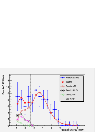
FIG. 1.: Best fit to KamLAND data including geo-neutrinos with $[Th]/[U]=3.8$ (low-LMA). The various contributions to the sum spectrum are shown as derived by the fit, which gives $N(U+Th)=9.9\pm 6.2$. The dotted vertical line corresponds to $2.6\,MeV$.

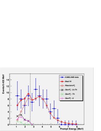
FIG. 2.: Second best fit to KamLAND data including geo-neutrinos with $[Th]/[U]=3.8$ (high-LMA). $N(U+Th)$ corresponds to $8.4\pm 5.9$.

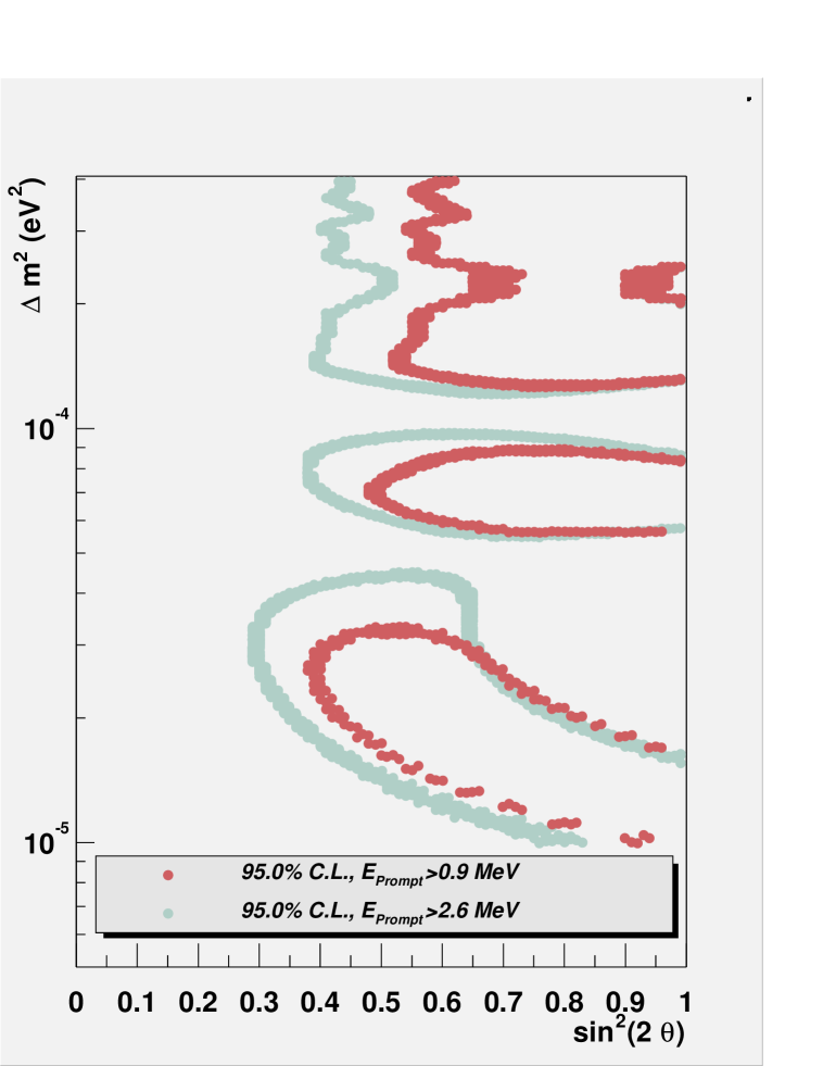
FIG. 3.: Comparison of the 95% C.L. allowed areas with and without geo-neutrinos constraint. The light-gray region is allowed analyzing the spectrum with an energy threshold of $2.6\,MeV$, while the dark-gray region is allowed including the full spectrum and constraining to $[Th]/[U]=3.8$.

REFERENCES

- [1] K. Eguchi et al., KamLAND Collaboration, hep-ex/0212021.
- [2] G. Fiorentini F. Mantovani and B. Ricci, nucl-ex/0212008.
- [3] Landolt-Börnstein, “Numerical data and functional relationships in science and technology”, New Series, Group IV vol. 3a, Springer-Verlag, Berlin 1993. http://www.landolt-boernstein.com/; http://ik3frodo.fzk.de/beer/pub/PB 198-203.pdf.
- [4] E. Anders and N. Grevesse, Geoch. Cosmoch. Acta, 53 (1989) 197.
- [5] R.S. Raghavan et al. , Phys. Rev. Lett. 80 (1998) 635.
- [6] C.G. Rothschild, M.C. Chen and F.P. Calaprice, nucl-ex/9710001. Geophy. Research Lett. 25 (1998) 1083.
- [7] G. Alimonti et al., BOREXINO Collaboration, Science and Technology of BOREXINO, Astropart.Phys. 16 (2002) 205-234.
- [8] G.L. Fogli et al., hep-ph/0112127.
- [9] M. Maltoni, T Schwetz and J.W.F. Valle, hep-ph/012129.
- [10] J.N. Bahcall, M.C. Gonzales-Garcia and C. Penya-Garay, hep-ph/0212147.
- [11] H. Nunokawa et al., hep-ph/0212202.
- [12] P. Aliani et al., hep-ph/0212212.
- [13] P.C. de Holanda and A.Yu. Smirnov, hep-ph/0212270.
- [14] V. Barger and D. Marfatia, hep-ph/0212126.
- [15] G.Harmann and K.H. Wedepohl, Geoch. et Cosm. Acta 57 (1993) 1761.
- [16] T.A. Ahrens ed, “Global Earth Physics: a handbook of physical constants”, American Geophysical Union, Washington, 1995.
- [17] P. Vogel and J. Beacom, Phys. Rev. D 60 (1999) 053003. C. Bemporad, G. Gratta, P. Vogel, Rev. Mod. Phys. 74 (2002) 297.
- [18] H. Behrens and J. Janecke, “Numerical tables for beta decay and electron capture”, Springer-Verlag, Berlin, 1969.
- [19] S. Schönert, T. Lasserre and L. Oberauer, hep-ex/0203013, Astrop. Phys. (2003) in print.
- [20] W.H. Press et al., “Numerical recipes”, Cambridge University Press, p. 689 (2002).