Deconstruction and Bilarge Neutrino Mixing

Abstract

We present a model for lepton masses and mixing angles using the deconstruction setup, based on a non-Abelian flavor symmetry which is a split extension of the Klein group $Z_{2}\times Z_{2}$. The symmetries enforce an approximately maximal atmospheric mixing angle $\theta_{23}$, a nearly vanishing reactor mixing angle $\theta_{13}$, and the hierarchy of charged lepton masses. The charged lepton mass spectrum emerges from the Froggatt-Nielsen mechanism interpreted in terms of deconstructed extra dimensions compactified on $\mathcal{S}^{1}$. A normal neutrino mass hierarchy arises from the coupling to right-handed neutrinos propagating in latticized $\mathcal{S}^{1}/Z_{2}$ orbifold extra dimensions. Here, the solar mass squared difference $\Delta m_{\odot}^{2}$ is suppressed by the size of the dynamically generated bulk manifold. Without tuning of parameters, the model yields the solar mixing angle $\theta_{12}={\rm arctan}\>1/\sqrt{2}$. Thus, the obtained neutrino masses and mixing angles are all in agreement with the Mikheyev–Smirnov–Wolfenstein large mixing angle solution of the solar neutrino problem.

1 Introduction

The standard model of elementary particle physics (SM), minimally extended by massive Majorana neutrinos, contains 22 fermion mass and mixing parameters (6 quark masses, 6 lepton masses, 3 CKM mixing angles [1, 2], 3 MNS mixing angles [3], 2 Dirac $\mathcal{CP}$ violation phases, and 2 Majorana phases). In four-dimensional (4D) gauge theories the fermion masses and mixing angles result from Yukawa couplings between fermions and scalars. However, even in 4D grand unified theories (GUTs) the Yukawa couplings are described by many free parameters and one therefore often assumes that the structure of the Yukawa coupling matrices is dictated by a sequentially broken flavor symmetry. Indeed, since the 4D Yukawa couplings become calculable in higher dimensional gauge theories [4], the effective fermion mass matrices emerging after dimensional reduction should actually be highly predictable from symmetries or the topology of internal space [5].

At first sight, the hierarchical structure of CKM angles and charged fermion masses suggests an underlying non-Abelian flavor symmetry group which essentially acts only on the first and second generations [6]. However, in these theories it is difficult to obtain exact predictions compatible with recent atmospheric [8, 9] and solar [10, 11] neutrino experimental results which prefer the Mikheyev-Smirnov-Wolfenstein (MSW) [12] large mixing angle (LMA) solution of the solar neutrino problem [13]. In fact, the KamLAND [14] reactor neutrino experiment has recently confirmed the MSW LMA solution at a significant level [15, 16, 17, 18]. In the “standard” parameterization, the MSW LMA solution tells us that the leptons obey a bilarge mixing in which the solar mixing angle $\theta_{12}$ is large, but not close to maximal, the atmospheric mixing angle $\theta_{23}$ is close to maximal, and the reactor mixing angle $\theta_{13}$ is small.

By assuming only Abelian $U(1)$ [19] or $Z_{n}$ [20] symmetries one finds that the atmospheric mixing angle may be large but cannot be enforced to be close to maximal. Thus, a natural close to maximal $\nu_{\mu}$-$\nu_{\tau}$-mixing can be interpreted as a strong hint for some non-Abelian flavor symmetry acting on the 2nd and 3rd generations [21, 22, 23]. Neutrino mass models which give large or maximal solar and atmospheric mixing angles by assigning the 2nd and 3rd generations quantum numbers of the symmetric groups $S_{2}$ [24] or $S_{3}$ [25] have, in general, difficulties to address the hierarchy of the charged lepton masses. This problem can be resolved in a supersymmetric model for degenerate neutrino masses by imposing the group $A_{4}$, the symmetry group of the tetrahedron [26]. In addition, this model predicts exactly $\theta_{23}=\frac{\pi}{4}$ from the $A_{4}$ symmetry and gives with some tuning of parameters the solar mixing angle $\theta_{12}$ of the MSW LMA solution. However, in unified field theories a normal hierarchical neutrino mass spectrum seems more plausible than an inverted or degenerate one [27]. A comparably simple way of accommodating the MSW LMA solution for normal hierarchical neutrino masses is provided in scenarios of single right-handed neutrino dominance [28].

Although unification in more than four dimensions can serve as a motivation for flavor symmetries, higher-dimensional gauge theories have dimensionful gauge couplings and are usually non-renormalizable. They require a truncation of Kaluza-Klein (KK) modes near some cut-off scale $M_{f}$ at which the perturbative regime of the higher-dimensional gauge theory breaks down. Recently, however, a new class of 4D gauge-invariant field theories for deconstructed or latticized extra dimensions has been proposed, which generate the physics of extra dimensions in their infrared limit [29, 30]. These theories are renormalizable and can thus be viewed as viable UV completions of some fundamental non-perturbative field theory, like string theory. In deconstruction, a number of replicated gauge groups is connected by fermionic or bosonic link variables. Since replicated gauge groups also frequently appear in models using the Froggatt-Nielsen mechanism [31, 32], it is straightforward to account for the generation of fermion mass matrices by deconstructed extra dimensional gauge symmetries.

In two previous works [33, 34] we have presented versions of a model for bilarge leptonic mixing based on a vacuum alignment mechanism for a strictly hierarchical charged lepton mass spectrum and an inverted neutrino mass hierarchy. As a result of the inverse hierarchical neutrino mass spectrum, we obtained the approximate relation $\theta_{12}=\frac{\pi}{4}-\theta_{13}$ and hence the lower bound $37^{\circ}\lesssim\theta_{12}$ on the solar mixing angle. In this paper, we now apply this vacuum alignment mechanism to a model for lepton masses and mixing angles which yields more comfortably the MSW LMA solution with normal hierarchical neutrino masses. Specifically, the lepton mass hierarchies are generated by deconstructed extra-dimensional $U(1)$ gauge symmetries where the lattice-link variables are themselves subject to a discrete non-Abelian flavor symmetry.

The paper is organized as follows: in Section 2, we introduce our example field theory by briefly reviewing the periodic and the aliphatic model for deconstructed extra dimensions. In Section 3, we first assign the horizontal $U(1)$ charges, then we discuss the non-Abelian discrete flavor symmetry and examine its normal structure. Next, in Section 4, we construct the potential for the scalar link-variables of the latticized extra dimensions from the representations of the dihedral group $\mathscr{D}_{4}$. The vacuum structure which results from minimizing the scalar potential is determined and analyzed in Section 5. In Section 6, we describe the generation of the charged lepton masses via the vacuum alignment mechanism. Then, in Section 7, we study the neutrino mass matrix, determine the neutrino mass and mixing parameters and match the types of latticizations of the orbifold extra dimensions onto the presently allowed ranges for $\Delta m_{\odot}^{2}$ implied by recent KamLAND results. Finally, we present in Section 8 our summary and conclusions. In addition, Appendix A gives a brief review of the dihedral group $\mathscr{D}_{4}$ and in Appendix B the minimization of the scalar potential is explicitly carried out.

2 Deconstruction setups

2.1 The periodic model

Consider a 4D gauge-invariant field theory for deconstructed or latticized extra dimensions [29, 30]. Let the field theory for $j=1,2,\ldots$ be described by products $G^{j}=\Pi^{N_{j}}_{i=1}G^{j}_{i}$ of $U(1)$ gauge groups $G^{j}_{i}$, where $N_{j}$ is the total number of “sites” corresponding to $G^{j}$. In the “periodic model” [29], one associates with each pair of groups $G^{j}_{i}\times G^{j}_{i+1}$ a link-Higgs field $Q^{j}_{i}$ with charge $(+1,-1)$ under $G^{j}_{i}\times G^{j}_{i+1}$, where $i$ is periodically identified with $i+N_{j}$. For our example field theory we will assume one periodic model for each of the gauge groups $G^{1}$ and $G^{2}$ where the number of sites is $N_{1}=2$ and $N_{2}=4$. This field theory is conveniently represented by the “moose” [35] or “quiver” [36] diagrams in Figs. 1 and 2.

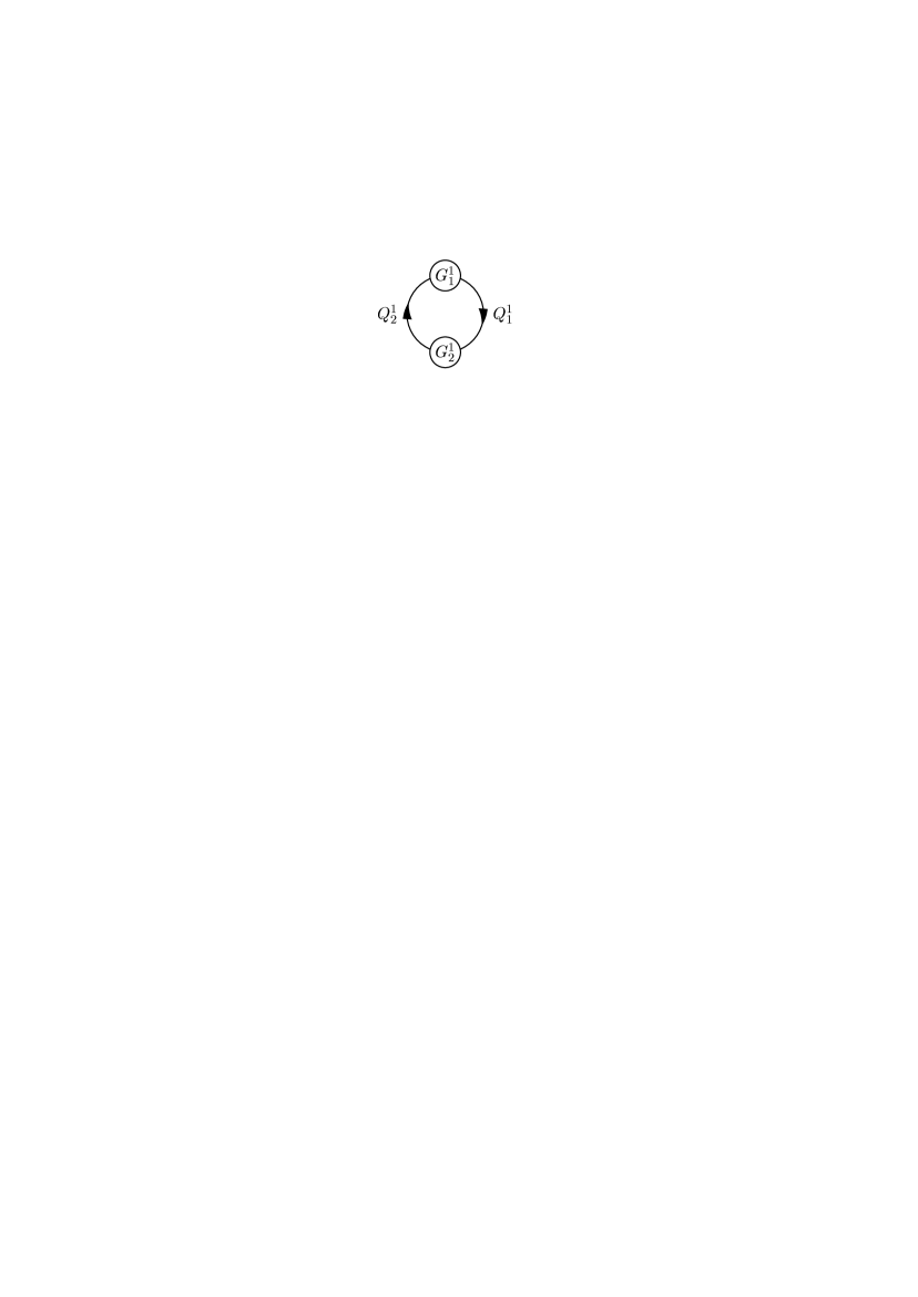
Figure 1: Moose diagram for the gauge group $G^{1}=\Pi^{2}_{i=1}G^{1}_{i}$.

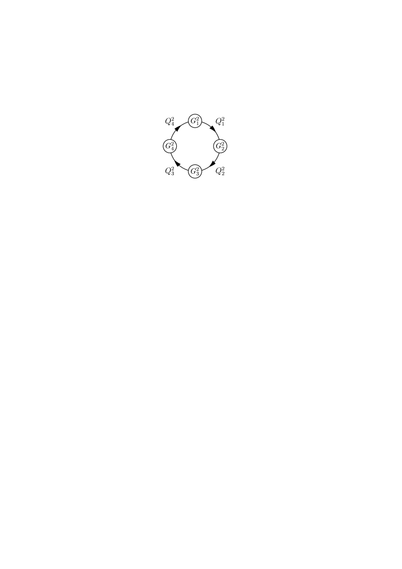
Figure 2: Moose diagram for the gauge group $G^{2}=\Pi_{i=1}^{4}G^{2}_{i}$.

Restricting for the present to a single product gauge group $G^{j}$ with $N_{j}=N$ sites, we can drop the index $j$ and write the Lagrangian in the periodic model as

$${\mathscr{L}}=-\frac{1}{4}\sum_{i=1}^{N}F_{i\mu\nu}F^{i\mu\nu}+\sum_{i=1}^{N}\left(D_{\mu}Q_{i}\right)^{\dagger}D^{\mu}Q_{i},$$ (1)

where $F_{i\mu\nu}=\partial_{\mu}A_{i\nu}-\partial_{\nu}A_{i\mu}$ is the 4D field strength and the covariant derivative is defined by

$$D_{\mu}Q_{i}=(\partial_{\mu}-{\rm i}g_{i}A_{i\mu}+{\rm i}g_{i+1}A_{(i+1)\mu})Q_{i}.$$ (2)

where $g_{i}$ is the dimensionless coupling constant of the gauge group $G$ at the $i$th site. For simplicity, it is assumed that all gauge couplings are equal,

$$g_{1}=g_{2}=\ldots=g_{N}\equiv g.$$ (3)

When the $Q_{i}$ aquire after spontaneous symmetry breaking (SSB) universal vacuum expectation values (VEVs) and each field becomes a non-linear $\sigma$-model field

$$Q_{i}\rightarrow v\>{\rm exp}({\rm i}\alpha_{i}/v),$$ (4)

the full gauge symmetry is higgsed to the diagonal $U(1)$ and it is seen that the Lagrangian in Eq. (1) describes a 4+1 dimensional $U(1)$ gauge theory on a flat background, where only the fifth dimension has been latticized. The lattice spacing $a$ and circumference $R$ of the fifth dimension are $a=1/(gv)$ and $R=N/(gv)$, whereas the 5D gauge coupling $g_{5}$ is given by $1/g_{5}^{2}=1/(ag^{2})$ [29, 37]. (In the model with free boundary conditions [30] generic gauge couplings and non-universal VEVs introduce an overall non-trivial warp factor [38, 39], resulting, e.g., in a Randall-Sundrum model [40].) Implicitly, we identify the link-Higgs fields with the continuum Wilson lines

$$Q_{i}(x^{\mu})={\rm exp}\left({\rm i}\int_{ia}^{(i+1)a}{{\rm d}x^{5}\>A_{5}(x^{\mu},x^{5})}\right),$$ (5)

where $(x^{\mu},x^{5})$ are the bulk coordinates and $A_{5}$ is the fifth component of the bulk gauge field associated with the gauge group $G$. The gauge boson mass matrix takes the form

$$\sum_{i=1}^{N}g^{2}v^{2}(A_{i\mu}-A_{(i+1)\mu})(A_{i}^{\mu}-A_{i+1}^{\mu})$$ (6)

and is of the type of a nearest neighbor coupled oscillator Hamiltonian. In the case of $N=4$, for example, the mass matrix for the gauge bosons reads

$$g^{2}v^{2}\left(\begin{matrix}2&-1&0&-1\\ -1&2&-1&0\\ 0&-1&2&-1\\ -1&0&-1&2\end{matrix}\right).$$ (7)

In general [29], the gauge boson mass matrix yields a mass spectrum labeled by an integer $k$ satisfying $-N/2<k\leq N/2$,

$$M_{k}^{2}=4g^{2}v^{2}{\rm sin}^{2}\left(\frac{\pi k}{N}\right)\equiv\left(\frac{2}{a}\right)^{2}{\rm sin}^{2}\left(\frac{p_{5}a}{2}\right),$$ (8)

where $p_{5}\equiv 2\pi k/R$ is the discrete 5D momentum. For small $|k|$ the masses are

$$M_{k}\simeq|p_{k}|=\frac{2\pi|k|}{R},\quad|k|\ll N/2,$$ (9)

which is exactly the KK spectrum of a 5D gauge theory compactified on $\mathcal{S}^{1}$ with circumference $R=N/(gv)$. The zero mode corresponds to the unbroken, diagonal $U(1)$. Hence, at energies $E\ll gv/N$ we observe an ordinary 4D gauge theory, in the range $gv/N<E<gv$ the physics is that of an extra dimension, and for $E\gg gv$ an unbroken $U(1)^{N}$ gauge theory in four dimensions is recovered.

2.2 The aliphatic model for fermions

The “aliphatic model” [30] for some product gauge group $G^{j}$ $(j=3,4,\ldots)$, as defined in Sec. 2.1, is obtained from the periodic model by setting $Q^{j}_{N_{j}}=0$ which yields a linear system with free boundary conditions. For this type of latticization we will consider $N_{j}$ SM singlet Dirac fermions $\Psi^{j}_{n}\>(n=1,\ldots,N_{j})$, each of which carries an associated $G^{j}_{n}$ charge $-1$. The SM singlet Higgs fields $Q^{j}_{n}\>(n=1,\ldots N_{j})$ which are assigned the $G^{j}_{n}\times G^{j}_{n+1}$ charges $(+1,-1)$ specify the allowed couplings between the fermions. Restricting here to a single product gauge group $G^{j}$ we may in this section drop the index $j$ for the rest of the discussion. The moose diagram for the aliphatic model is shown in Fig. 3.

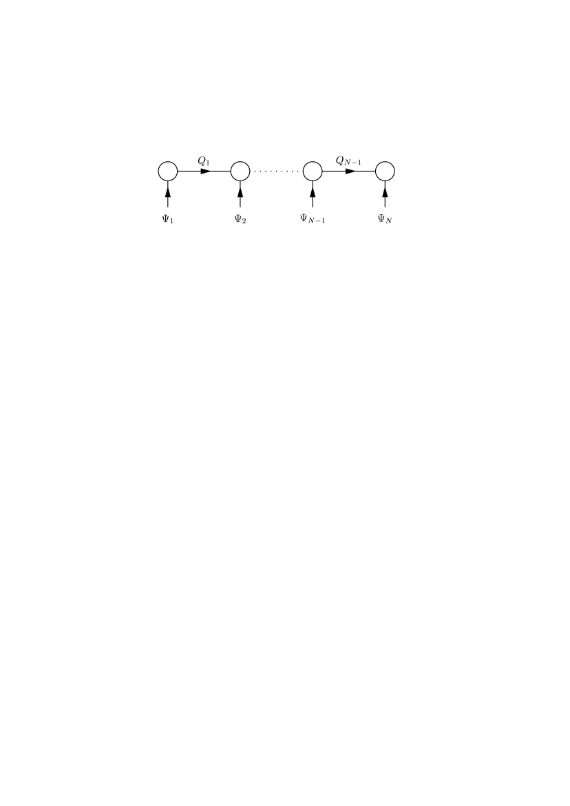
Figure 3: Moose diagram for bulk vector fields and fermions in the aliphatic model.

We will denote by $\Psi_{nL}$ and $\Psi_{nR}$ the left- and right-handed chiral components of $\Psi_{n}$ respectively. To engineer chiral fermion zero modes from compactification of the 5th dimension, one can impose discretized versions of the Neumann and Dirichlet boundary conditions $\Psi_{NL}-\Psi_{(N-1)L}=0$ and $\Psi_{1R}=\Psi_{NR}=0$ which explicitly break the Lorentz group in five dimensions. Using the transverse lattice technique [41, 42] the relevant mass and mixing terms of $\Psi_{nL}$ and $\Psi_{mR}$ then read [30, 38]

$${\mathscr{L}}_{1} = M_{f}\sum_{n=2}^{N-1}\left[\overline{\Psi}_{nL}\left(\frac{Q^{\dagger}_{n+1}}{v}\Psi_{(n+1)R}-\Psi_{nR}\right)-\overline{\Psi}_{nR}\left(\Psi_{nL}-\frac{Q_{n}}{v}\Psi_{(n-1)L}\right)\right]$$ (10)

$$+M_{f}\overline{\Psi}_{1L}\Psi_{2R}+{\rm h.c.},$$

where $v\equiv\langle Q_{n}\rangle$ for $n=1,\ldots,N-1$, i.e., we have universal VEVs. In fact, Eq. (10) is the Wilson-Dirac action [43] for a transverse extra dimension which reproduces the 5D continuum theory in the limit of vanishing lattice spacing. Clearly, this tacitly presupposes a specific functional measure for the link variables in question which may, however, no longer be a necessary choice when the lattice spacing is finite [42]. After SSB the mixed mass terms of the chiral fermions are

$${\mathscr{L}}_{\rm mass} = M_{f}\sum_{n=2}^{N-1}\left[\overline{\Psi}_{nL}(\Psi_{(n+1)R}-\Psi_{nR})-\overline{\Psi}_{nR}(\Psi_{nL}-\Psi_{(n-1)L})\right]$$ (11)

$$+M_{f}\overline{\Psi}_{1L}\Psi_{2R}+{\rm h.c.}$$

$$= (\overline{\Psi}_{1L},\ldots,\overline{\Psi}_{(N-1)L})^{T}{\mathcal{M}}_{1}(\Psi_{2R},\ldots,\Psi_{(N-1)R})+{\rm h.c.},$$

where the $(N-1)\times(N-2)$ fermion mass matrix ${\mathcal{M}}_{1}$ is on the form

$${\mathcal{M}}_{1}=M_{f}\left(\begin{matrix}1&0&0&\cdots&0&0\\ -1&1&0&\cdots&0&0\\ \vdots&\vdots&\vdots&&\vdots&\vdots\\ 0&0&0&\cdots&-1&1\\ 0&0&0&\cdots&0&-1\end{matrix}\right).$$ (12)

Diagonalizing the $(N-2)\times(N-2)$ matrix ${\mathcal{M}}_{1}^{\dagger}{\mathcal{M}}_{1}$ gives for the mass eigenvalues of the right-handed fermions

$$M_{nR}=2M_{f}\>{\rm sin}\left(\frac{n\pi}{2(N-1)}\right),\quad n=1,2,\ldots,N-2,$$ (13)

where the associated mass eigenstates $\tilde{\Psi}_{kR}$ are related to $\Psi_{nL}$ by [30]:

$$\Psi_{nR}=\sqrt{\frac{N-1}{2}}\sum_{k=1}^{N-2}{\rm sin}\left(n\frac{k\pi}{N-1}\right)\tilde{\Psi}_{kR}.$$ (14)

The diagonalization of the $(N-1)\times(N-1)$ matrix ${\mathcal{M}}_{1}{\mathcal{M}}_{1}^{\dagger}$ yields masses for the left-handed fermions, which are identical with the gauge boson masses,

$$M_{nL}=2M_{f}\>{\rm sin}\left(\frac{n\pi}{2(N-1)}\right),\quad n=0,1,\ldots,N-2,$$ (15)

and in terms of the associated the mass eigenstates $\tilde{\Psi}_{kL}$ we have [30]:

$$\Psi_{nL}=\sqrt{\frac{N-1}{2}}\sum_{k=0}^{N-2}{\rm cos}\left(\frac{2n+1}{2}\frac{k\pi}{N-1}\right)\tilde{\Psi}_{kL}.$$ (16)

Setting $M_{f}=\frac{N-1}{R}$ and taking the limit $n\ll N$ the linear KK spectrum of a 5D fermion in an orbifold extra dimension $\mathcal{S}^{1}/Z_{2}$ is reproduced. Up to an overall scale factor of 2, the periodic and the aliphatic model generate identical KK mass spectra for bulk vector fields, with the number of KK modes doubled in the periodic case [44].

3 Horizontal charges

In 5D continuum theories hierarchical Yukawa coupling matrix textures have been successfully generated [45]. Hierarchical Yukawa matrices have also been obtained in deconstructed warped geometries [46]. In our deconstruction setup of Sec. 2 let us now consider an extension of the SM, where the lepton masses arise from higher-dimensional operators [47], partly via the Froggatt-Nielsen mechanism.

3.1 $U(1)$ charges

We denote the left-handed SM lepton doublets as $L_{\alpha}=(\nu_{\alpha L}\>e_{\alpha L})^{T}$ and the right-handed charged leptons as $E_{\alpha}$, where $\alpha=e,\mu,\tau$ is the flavor index. For simplicity, we will assume the electroweak scalar sector to consist only of the SM Higgs doublet $H$. In order to account for the neutrino masses, we will additionally assume three SM singlet scalar fields $\xi_{0},\xi_{1},$ and $\xi_{2},$ as well as three heavy SM singlet Dirac neutrinos $F_{e},F_{\mu},$ and $F_{\tau}$. Since these Dirac neutrinos are supposed to have masses of the order of the GUT scale $\simeq 10^{15}\>{\rm GeV}$, they will account for the smallness of the neutrino masses via the seesaw mechanism [48, 49]. Furthermore, the standard Froggatt-Nielsen mechanism is implied in the charged lepton sector by the presence of heavy fundamental charged fermion messengers. The electron, muon, and tau masses will be denoted by $m_{e},m_{\mu},$ and $m_{\tau}$, respectively.

In models of inverted neutrino mass hierarchy, a small reactor mixing angle $\theta_{13}$ can be understood in terms of a softly broken $\tilde{L}_{e}-\tilde{L}_{\mu}-\tilde{L}_{\tau}$ lepton number [50]. Analogously, we assume that our example field theory contains a product $G_{L}\times G_{R}$ of two extra $U(1)$ gauge symmetries $G_{L}$ and $G_{R}$ which distinguish the 1st generation from the 2nd and 3rd generations, but act also on $\xi_{0},\xi_{1},\xi_{2},$ and the scalar link fields of the product gauge groups $G^{1}=\Pi^{2}_{i=1}G^{1}_{i}$ and $G^{2}=\Pi^{4}_{i=1}G^{2}_{i}$. The $G_{L}\times G_{R}$ charge assignment is shown in table 1.

	$G_{L}\times G_{R}$
$L_{e}$	$(+2,-2)$
$E_{e},F_{e},\xi_{0}$	$(-2,+2)$
$L_{\mu},L_{\tau},Q^{1}_{1},Q^{2}_{1},\xi_{1},\xi_{2}$	$(+1,0)$
$F_{\mu},F_{\tau}$	$(-1,0)$
$E_{\mu},E_{\tau}$	$(0,+1)$
$Q^{1}_{2},Q^{2}_{4}$	$(0,-1)$

Table 1: Assignment of the horizontal $U(1)^{2}$ charges to the different fields. The fields not shown here transform trivially under $G_{L}\times G_{R}$.

Note that the $G_{L}\times G_{R}$ symmetry is anomalous. However, anomalous $U(1)$ charges are expected to arise in string theory and must be canceled by the Green-Schwarz mechanism [51].

Let us now suppose that the charges of the product gauge groups $G_{L}\times G_{R}$, $G^{1}$, and $G^{2}$ are approximately conserved in the charged lepton sector, implying the generation of hierarchical charged lepton mass terms via the Froggatt-Nielsen mechanism. Furthermore, we assume that the fields $\xi_{0},\xi_{1},$ and $\xi_{2}$ carry nonzero $G^{3}$ and $G^{4}$ quantum numbers, respectively, while the fundamental charged Froggatt-Nielsen messengers transform only trivially under $G^{3}$ and $G^{4}$. As a consequence, the fields $\xi_{0},\xi_{1},$ and $\xi_{2}$ can be discarded in the discussion of the generation of the charged lepton masses (see also Sec. 7.1). Then, we conclude from table 1 that gauge-invariance under the product gauge group $G_{L}\times G_{R}\times G^{1}\times G^{2}$ allows in the $\mu$-$\tau$-subsector only two general types of non-renormalizable leading-order charged lepton mass terms: One operator of the dimension $4+N_{1}=6$ and one of the dimension $4+N_{2}=8$. The corresponding Froggatt-Nielsen-type diagrams are shown in Fig. 4. Note here, that the effective Yukawa couplings of the dimension-six and dimension-eight operators arise from the link fields of the deconstructed extra-dimensional gauge groups $G^{1}$ and $G^{2}$, respectively.

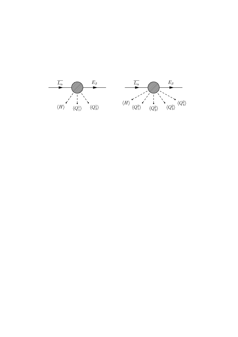
Figure 4: Lowest-dimensional Yukawa interactions generating for $\alpha,\beta=\mu,\tau$ the charged lepton mass terms in the $\mu$-$\tau$-subsector.

3.2 Discrete charges

It has been pointed out, that a naturally maximal $\nu_{\mu}$-$\nu_{\tau}$-mixing is a strong hint for an underlying non-Abelian flavor symmetry acting on the 2nd and 3rd generations [21, 22, 23]. Seemingly, this flavor symmetry is unlikely to be a continuous global symmetry because of the absence of such symmetries in string theory [52]. From the point of view of string theory, however, it is interesting to analyze conventional grand unification in connection with discrete symmetries since these might provide a solution to the doublet-triplet splitting problem [53, 54, 55]. Additionally, discrete symmetries can ensure an approximately flat potential for the GUT breaking fields in order to avoid fast proton decay [56]. Moreover, it has recently been demonstrated that the appropriate discrete symmetries of the low-energy theory can be naturally obtained in deconstructed models with very coarse latticization, when the lattice link variables are themselves subject to a discrete symmetry [55]. It is interesting to note, that although a classical lattice gauge theory based on a system of link fields which are elements of some discrete group has no continuum limit, this does not necessarily carry over to the quantum theory.

Among the discrete symmetries that have been proposed in the context of the MSW LMA solution as a possible origin of an approximately maximal atmospheric mixing angle $\theta_{23}$ are the symmetric groups $S_{2}$ and $S_{3}$ acting on the 2nd and 3rd generations of leptons [25, 24]. While this can indeed give an approximately maximal $\nu_{\mu}$-$\nu_{\tau}$-mixing, the hierarchical charged lepton mass spectrum is typically not produced in these types of models, since they rather yield masses of the muon and tau that are of the same order of magnitude. However, when we add to the regular representation of $S_{2}$ in the $\mu$-$\tau$-flavor basis the generator ${\rm diag}(-1,\>1)$, one obtains the vector representation of the dihedral group $\mathscr{D}_{4}$, which is non-Abelian (see App. A). Since the generator ${\rm diag}(-1,\>1)$ distinguishes between $L_{\mu}$ and $L_{\tau}$ it may serve as a possible source for the charged lepton mass hierarchy, which breaks the permutation symmetry $S_{2}\subset\mathscr{D}_{4}$ characteristic for the $\nu_{\mu}$-$\nu_{\tau}$-sector. Clearly, if the charged lepton masses arise from the Froggatt-Nielsen mechanism, we will have to expect that the underlying symmetry is actually equivalent to a group extension of some subgroup of $\mathscr{D}_{4}$, presumably a suitable subgroup of some replicated product of $\mathscr{D}_{4}$-factors.

Motivated by these general observations, we will take here the view, that an approximately maximal atmospheric mixing angle $|\theta_{23}-\frac{\pi}{4}|\ll 1$ is due to a non-Abelian discrete symmetry $\mathscr{G}$ which is a group extension based on the generators of the dihedral group $\mathscr{D}_{4}$ under which the leptons of the 2nd and 3rd generation, the scalars $\xi_{1},\xi_{2},$ and the scalar link variables of the deconstructed extra-dimensional gauge symmetries $G^{1}=\Pi^{2}_{i=1}G^{1}_{i}$ and $G^{2}=\Pi^{4}_{i=1}G^{2}_{i}$ transform non-trivially. Specifically, we suppose that in the defining representation $\mathcal{D}$ the group $\mathscr{G}$, which is a subgroup of the four-fold (external) product group $\mathscr{D}_{4}\times\mathscr{D}_{4}\times\mathscr{D}_{4}\times\mathscr{D}_{4}$, can be written as a sequence

$$\mathcal{D}(g)\equiv{\rm diag}\left[\begin{matrix}D_{1}(g),&D_{2}(g),&D_{3}(g),&D_{4}(g)\end{matrix}\right]\quad g\in\mathscr{G},$$ (17)

where each element $g\in\mathscr{G}$ is associated with four (in general different) $2\times 2$ charge operators $D_{i}(g)$ $(i=1,2,3,4)$ which have values in the vector representation of $\mathscr{D}_{4}$. Clearly, for given $i=1,2,3,4$ the set of all operators $\{D_{i}(g):g\in\mathscr{G}\}$ forms a subrepresentation of $\mathscr{G}$ which we will call $D_{i}$. Now, using the notation of App. A we suppose that $\mathscr{G}$ is represented by four generators with following $\mathscr{D}_{4}$-charge structure

$$\mathcal{D}(a_{1}) \equiv {\rm diag}\left[\begin{matrix}D(C_{b}),&D(E),&D(C_{b^{\prime}}),&D(C_{b^{\prime}})\end{matrix}\right],$$ (18a)

$$\mathcal{D}(a_{2}) \equiv {\rm diag}\left[\begin{matrix}D(C_{b^{\prime}}),&D(C_{b^{\prime}}),&D(C_{b}),&D(E)\end{matrix}\right],$$ (18b)

$$\mathcal{D}(a_{3}) \equiv {\rm diag}\left[\begin{matrix}D(E),&D(E),&D(C_{b}),&D(C_{b})\end{matrix}\right],$$ (18c)

$$\mathcal{D}(a_{4}) \equiv {\rm diag}\left[\begin{matrix}D(C_{b}),&D(C_{b}),&D(E),&D(E)\end{matrix}\right],$$ (18d)

where $a_{1},a_{2},a_{3},a_{4}\in\mathscr{G}$ are the corresponding abstract generators. Note that these operators are characterized by a one-to-one-correspondence $\mathcal{D}(a_{1})\leftrightarrow\mathcal{D}(a_{2})$ and $\mathcal{D}(a_{3})\leftrightarrow\mathcal{D}(a_{4})$ under the permutation of the upper-left and the lower-right $4\times 4$-matrices. As will be shown in Sec. 3.3, by factoring the subrepresentation $D_{i}$ for any $i=1,2,3,4$ with respect to its kernel $\mathcal{N}_{i}$ we obtain a representation of the factor group $\mathscr{G}/\mathcal{N}_{i}$ that is isomorphic with $\mathscr{D}_{4}$. This implies, of course, that all four subrepresentations $D_{1},D_{2},D_{3},$ and $D_{4}$ are two-dimensional irreducible representations (irreps) of $\mathscr{G}$. From App. A it is seen, that in an appropriate basis the generators of Eqs. (18) can be explicitly written as

$$\mathcal{D}(a_{1}) \equiv {\rm diag}\left[\begin{matrix}\left(\begin{matrix}-1&0\\ 0&1\end{matrix}\right),&\left(\begin{matrix}1&0\\ 0&1\end{matrix}\right),&\left(\begin{matrix}0&1\\ 1&0\end{matrix}\right),&\left(\begin{matrix}0&1\\ 1&0\end{matrix}\right)\end{matrix}\right],$$ (19a)

$$\mathcal{D}(a_{2}) \equiv {\rm diag}\left[\begin{matrix}\left(\begin{matrix}0&1\\ 1&0\end{matrix}\right),&\left(\begin{matrix}0&1\\ 1&0\end{matrix}\right),&\left(\begin{matrix}-1&0\\ 0&1\end{matrix}\right),&\left(\begin{matrix}1&0\\ 0&1\end{matrix}\right)\end{matrix}\right],$$ (19b)

$$\mathcal{D}(a_{3}) \equiv {\rm diag}\left[\begin{matrix}\left(\begin{matrix}1&0\\ 0&1\end{matrix}\right),&\left(\begin{matrix}1&0\\ 0&1\end{matrix}\right),&\left(\begin{matrix}-1&0\\ 0&1\end{matrix}\right),&\left(\begin{matrix}-1&0\\ 0&1\end{matrix}\right)\end{matrix}\right],$$ (19c)

$$\mathcal{D}(a_{4}) \equiv {\rm diag}\left[\begin{matrix}\left(\begin{matrix}-1&0\\ 0&1\end{matrix}\right),&\left(\begin{matrix}-1&0\\ 0&1\end{matrix}\right),&\left(\begin{matrix}1&0\\ 0&1\end{matrix}\right),&\left(\begin{matrix}1&0\\ 0&1\end{matrix}\right)\end{matrix}\right].$$ (19d)

With respect to $\mathcal{D}$ we will combine the left- and right-handed SM leptons as well as the Dirac neutrinos of the 2nd and 3rd generations into the $\mathscr{G}$-doublets $\mathbf{2}_{\ell}\equiv(L_{\mu},\>L_{\tau})^{T}$, $\mathbf{2}_{E}\equiv(E_{\mu},E_{\tau})^{T}$, and $\mathbf{2}_{F}\equiv(F_{\mu},\>F_{\tau})^{T}$, respectively. The fermionic doublets $\mathbf{2}_{\ell}$ and $\mathbf{2}_{F}$ as well as the scalars $\xi_{1}\equiv\left(\xi_{1a},\>\xi_{1b}\right)^{T}$ and $\xi_{2}\equiv\left(\xi_{2a},\>\xi_{2b}\right)^{T}$ are all put into the doublet representation $D_{1}$. Next, the generalized Wigner-Eckart theorem tells us that the effective Yukawa interaction matrix spanned by $\mathbf{2}_{\ell}$ and $\mathbf{2}_{E}$ in the $\mu$-$\tau$-subsector of the charged leptons is identical with a linear combination of sets of irreducible Yukawa tensor operators. If the irreducible Yukawa tensor operators take their values in the vector representation of $\mathscr{D}_{4}$, it is clear from App. A, that the hierarchy $m_{\mu}\ll m_{\tau}$ is only possible if $\mathbf{2}_{E}$ transforms according to an irrep of $\mathscr{G}$ which is inequivalent with $D_{1}$. We will therefore put $\mathbf{2}_{E}$ into the irrep $D_{2}$ which is inequivalent with $D_{1}$ and note that the large subgroup of $\mathscr{G}$ generated by $\mathcal{D}(a_{2}),\mathcal{D}(a_{3}),$ and $\mathcal{D}(a_{4})$ acts diagonally on $\mathbf{2}_{\ell}$ and $\mathbf{2}_{E}$.

In Sec. 3.1 we have seen that $G_{L}\times G_{R}\times G^{1}\times G^{2}$ gauge-invariance requires the possible lowest-dimensional effective Yukawa interactions between $\mathbf{2}_{\ell}$ and $\mathbf{2}_{E}$ to be identical with the dimension-six and dimension-eight Froggatt-Nielsen-type operators displayed in Fig. 4. In theory space, we can therefore identify the sets of irreducible Yukawa tensor operators spanned by $\mathbf{2}_{\ell}$ and $\mathbf{2}_{E}$ with the Wilson loops around the plaquettes associated with the deconstructed extra-dimensional gauge-symmetries $G^{1}$ and $G^{2}$: The dimension-six and dimension-eight operators correspond to the Wilson loops around the moose diagrams of $G^{1}$ (Fig. 5) and $G^{2}$ (Fig. 6), respectively.

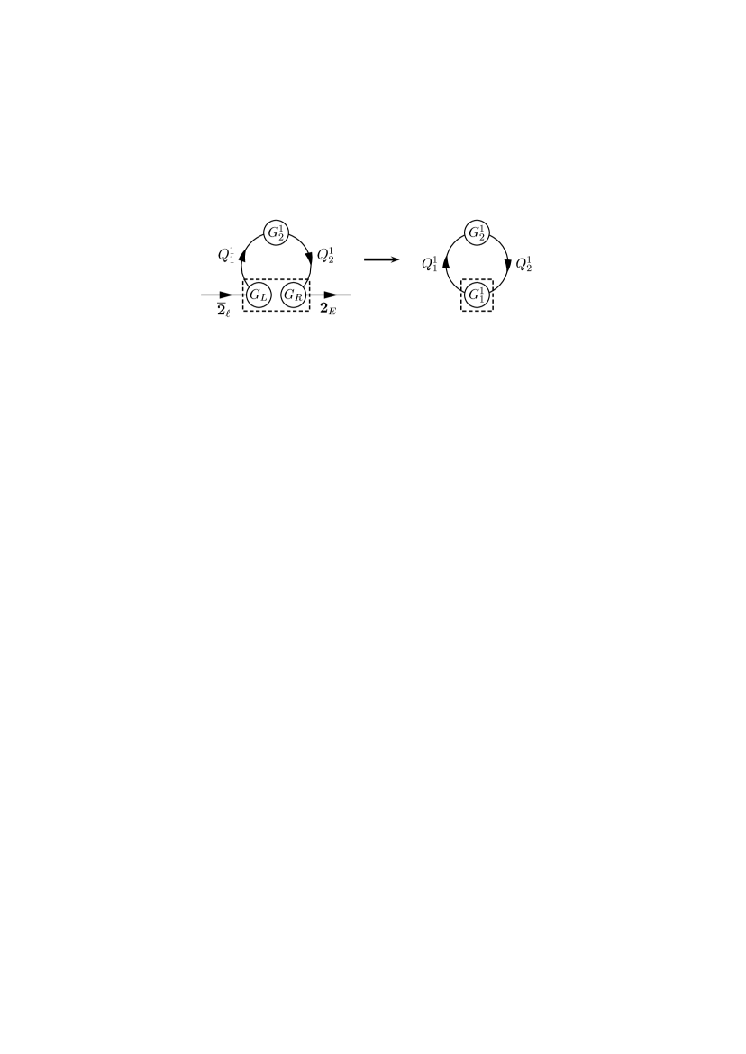
Figure 5: Contour in theory space which generates the dimension-six mass operator in Fig. 4 by connecting $\mathbf{2}_{\ell}$ and $\mathbf{2}_{E}$ via the link fields of $G^{1}$ (left panel). Formal contraction of the open fermion lines and $G_{L}\times G_{R}$ into $G^{1}_{1}$ (dashed boxes) exhibits the full $G^{1}$ gauge-invariance of the corresponding effective Yukawa couplings (right panel).

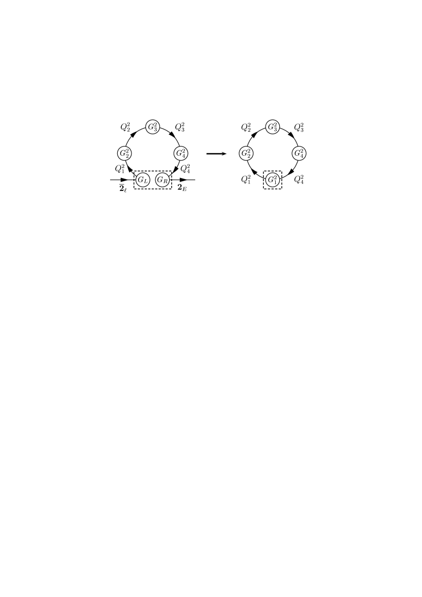
Figure 6: Contour in theory space which generates the dimension-eight mass operator in Fig. 4 by connecting $\mathbf{2}_{\ell}$ and $\mathbf{2}_{E}$ via the link fields of $G^{2}$ (left panel). Formal contraction of the open fermion lines and $G_{L}\times G_{R}$ into $G^{2}_{1}$ (dashed boxes) exhibits the full $G^{2}$ gauge-invariance of the corresponding effective Yukawa couplings (right panel).

Although the irreps $D_{1}$ and $D_{2}$ already determine the overall transformation properties of the Wilson loops under $\mathscr{G}$, there is still some ambiguity in the individual $\mathscr{G}$-charge assignment to the involved link-fields $Q^{1}_{1},Q^{1}_{2},$ and $Q^{2}_{1},Q^{2}_{2},Q^{2}_{3},Q^{2}_{4}$. Here, it is appealing to assume that all the scalar link fields of $G^{1}$ and $G^{2}$ transform according to some doublet subrepresentation of $\mathscr{G}$, which has the property that its lift is isomorphic with $\mathscr{D}_{4}$. Furthermore, a non-trivial Yukawa matrix structure requires that the products $\Pi_{i=1}^{2}Q^{1}_{i}$ and $\Pi_{i=1}^{4}Q^{2}_{i}$ are non-singlet representations of $\mathscr{G}$. Since each of the Wilson loops involves an even number of (two or four) link fields, we find from the multiplication rules in App. A that this can only be the case if each of the sets $\{Q^{1}_{1},Q^{1}_{2}\}$ and $\{Q^{2}_{1},Q^{2}_{2},Q^{2}_{3},Q^{2}_{4}\}$ contains at least two inequivalent irreps. This can be simply realized by putting, e.g., the 1st ($i=1$) link fields $Q^{1}_{1}$ and $Q^{2}_{1}$ into the doublet representation $D_{3}$ while the remaining link fields $Q^{1}_{2},Q^{2}_{2},Q^{2}_{3},$ and $Q^{2}_{4}$ all transform as doublets under $D_{4}$. Note again, that both $D_{3}$ and $D_{4}$ are characterized by a large common subgroup generated by $\mathcal{D}(a_{1}),\mathcal{D}(a_{3}),$ and $\mathcal{D}(a_{4}),$ which acts diagonally on all of the link fields. In component-form, the scalar ${\mathscr{G}}$-doublets will be written as $Q^{1}_{i}\equiv\left(q^{1}_{ia},\>q^{1}_{ib}\right)^{T}$, where $i=1,2,$ and $Q^{2}_{i}\equiv\left(q^{2}_{ia},\>q^{2}_{ib}\right)^{T}$, where $i=1,2,3,4$. To complete the $\mathscr{G}$-charge assignment, we suppose that the first generation fields $L_{e},E_{e},$ and $F_{e}$, as well as the scalar $\xi_{0}$ transform only trivially under $\mathscr{G}$, i.e., they are all put into the identity representation $I$ of $\mathscr{G}$. For the fermionic $\mathscr{G}$-singlets $L_{e},E_{e},$ and $F_{e}$ we will also choose the notation $\mathbf{1}_{e}\equiv L_{e}$, $\mathbf{1}_{E}\equiv E_{e}$, and $\mathbf{1}_{F}\equiv F_{e}$. The assignment of the fields to the irreps $D_{i}$ $(i=1,2,3,4)$ and $I$ is summarized in table 2.

$I$	$D_{1}$	$D_{2}$	$D_{3}$	$D_{4}$
$\mathbf{1}_{e},\mathbf{1}_{E},\mathbf{1}_{F},\xi_{0}$	$\mathbf{2}_{\ell},\mathbf{2}_{F},\xi_{1},\xi_{2}$	$\mathbf{2}_{E}$	$Q^{1}_{1},Q^{2}_{1}$	$Q^{1}_{2},Q^{2}_{2},Q^{2}_{3},Q^{2}_{4}$

Table 2: Assignment of the fermionic and scalar fields to the different irreps $D_{i}$ and $I$. Note that the scalar link fields transform according to their position in the “index space” of gauge groups.

In this subsection, we have presented the non-Abelian group $\mathscr{G}$ in terms of its generators which are motivated by phenomenology. In the following subsection we will examine in some more detail the structure of $\mathscr{G}$ through a descending series of normal subgroups, i.e., the normal structure.

3.3 Normal structure

In Sec. 3.2 the discrete group $\mathscr{G}$ has been constructed from the generators of the dihedral group $\mathscr{D}_{4}$. A standard way of gaining further information about $\mathscr{G}$ is to analyze a series of subgroups of $\mathscr{G}$, where each term is either normal in $\mathscr{G}$ or at least normal in the previous term. In general, if a subgroup $N$ of some group $G$ is normal in $G$ we will write $N\trianglelefteq G$.

We will denote by ${\mathcal{K}}_{1}$ the collection of all elements $g\in\mathscr{G}$ which obey $D_{1}(g)=\mathbbm{1}_{2}$, where $\mathbbm{1}_{2}$ is the $2\times 2$ unit matrix. Accordingly, we will define ${\mathcal{K}}_{2}$ as the set of all elements $g\in\mathscr{G}$ which obey $D_{1}(g)=D_{2}(g)=\mathbbm{1}_{2}$, and ${\mathcal{K}}_{3}$ as the set of all elements $g\in\mathscr{G}$ which obey $D_{1}(g)=D_{2}(g)=D_{3}(g)=\mathbbm{1}_{2}$. We therefore have the sequence

$${\mathcal{K}}_{3}\subset{\mathcal{K}}_{2}\subset{\mathcal{K}}_{1}\subset\mathscr{G},$$ (20)

where each subset is a group, actually an invariant subgroup of the embedding groups, for if $a\in{\mathcal{K}}_{i}$ $(i=1,2,3)$ is homomorphically mapped on the identity of the operator group $D_{1}\oplus\ldots\oplus D_{i}$, then so are all elements in its class. We therefore have $\mathcal{K}_{i+1}\trianglelefteq\mathcal{K}_{i}$ and $\mathcal{K}_{i}\trianglelefteq\mathscr{G}$ for every $i$, i.e., the subgroup series in Eq. (20) is in fact a normal series. From Eqs. (19) we find that for any $k\in{\mathcal{K}}_{2}$ the decomposition of $\mathcal{D}(k)$ into a product of the operators $\mathcal{D}(a_{i})$ $(i=1,2,3,4)$ necessarily involves each of the factors $\mathcal{D}(a_{1}),\mathcal{D}(a_{2}),$ and $\mathcal{D}(a_{4})$ an even number of times. In turn, this implies that the operators $D_{3}(k)$ and $D_{4}(k)$ are on diagonal form and can take their values only in the classes $E,C_{4}^{2},$ and $C_{2}(2)$ of the dihedral group $\mathscr{D}_{4}$ (see App. A). Since the number of elements in the classes $E,C^{2}_{4},$ and $C_{2}(2)$ is four, we conclude that the order of ${\mathcal{K}}_{2}$, which we will denote by $|\mathcal{K}_{2}|$, obeys $|\mathcal{K}_{2}|\leq 4$. Indeed, besides the unity, we find the three distinct elements $a_{3}$, $a_{1}a_{3}a_{1}$, and $(a_{1}a_{3})^{2}$ which are all contained in ${\mathcal{K}}_{2}$. Hence, $|\mathcal{K}_{2}|=4$ and we have

$${\mathcal{K}}_{2} \simeq \left\{{\rm diag}\left[D(E),D(E),D(E),D(E)\right],\right.$$ (21)

$$\>\>{\rm diag}\left[D(E),D(E),D(C_{a}),D(C_{a})\right],$$

$$\>\>{\rm diag}\left[D(E),D(E),D(C_{b}),D(C_{b})\right],$$

$$\>\>\left.{\rm diag}\left[D(E),D(E),D(C_{4}^{2}),D(C_{4}^{2})\right]\right\}.$$

Since ${\mathcal{K}}_{3}\subset{\mathcal{K}}_{2}$ the group ${\mathcal{K}}_{3}$ is trivial and contains only the identity of $\mathcal{D}$, as inspection of Eq. (21) shows. From Eq. (21) we find that $\mathcal{K}_{2}$ describes a 2-fold axis with a system of two 2-fold axes at right angle to it. Hence, $\mathcal{K}_{2}$ is isomorphic with the Klein group $Z_{2}\times Z_{2}\simeq\mathcal{K}_{2}$. In fact, the Klein group is one of the dihedral groups $Z_{2}\times Z_{2}\simeq\mathscr{D}_{2}$ (see App. A). With ${\mathcal{K}}_{2}$ explicitly given in Eq. (21) we can now easily construct a representation of the embedding group ${\mathcal{K}}_{1}\trianglerighteq\mathcal{K}_{2}$. First, note that for any $k\in{\mathcal{K}}_{1}$ the resolution of the operator $\mathcal{D}(k)$ into a product of the generators in Eq. (19) must involve $\mathcal{D}(a_{2})$ an even number of times. Hence, $D_{2}(k)$ is necessarily on diagonal form implying that the index of the subgroup ${\mathcal{K}}_{2}$ under the group ${\mathcal{K}}_{1}$ is at most four. In fact, the group ${\mathcal{K}}_{1}$ can be decomposed into (right) cosets in terms of

$${\mathcal{K}}_{1}\simeq{\mathcal{K}}_{2}+\sum_{i=1}^{3}{\mathcal{K}}_{2}\>b_{i},$$ (22)

where we can choose the different coset representatives to be $b_{1}=a_{1}a_{4}$, $b_{2}=a_{2}b_{1}a_{2}$, and $b_{3}=b_{2}b_{1}$. In other words, four elements of ${\mathcal{K}}_{1}$ are mapped on each element of the operator group corresponding to the representation of $\mathcal{K}_{1}$ subduced by $D_{2}$ (subduced representation) $D_{2}\downarrow\mathcal{K}_{1}$. Since the subgroup $\mathcal{K}_{2}\trianglelefteq\mathcal{K}_{1}$ is the kernel of $D_{2}\downarrow\mathcal{K}_{1}$, the operators $D_{2}(b_{i})$ $(i=1,2,3)$ from the (right) transversal allow us to identify the lift of $D_{2}\downarrow\mathcal{K}_{1}$ as the Klein group $Z_{2}\times Z_{2}$. As for the coset representatives don’t commute with the elements of ${\mathcal{K}}_{2}$ it follows that ${\mathcal{K}}_{1}$ is actually an (external) semi-direct product or split extension of $\mathcal{K}_{2}$ by $Z_{2}\times Z_{2}$. Hence, we can write

$${\mathcal{K}}_{1}\simeq(Z_{2}\times Z_{2})\rtimes_{\varphi}(Z_{2}\times Z_{2}),$$ (23)

where $\varphi$ is the mapping of $\mathcal{K}_{2}$ into the automorphism group of $\mathcal{K}_{2}$ which is determined by the particular choice of the generators in Eq. (18). The mapping $\varphi$ can be identified with the conjugation homomorphism of the corresponding internal semi-direct product describing the interaction of the two involved $Z_{2}\times Z_{2}$ subgroups inside $\mathscr{G}$. Now, the order of ${\mathcal{K}}_{1}$ is simply given by the product of the orders of the semi-direct factors, i.e., $|\mathcal{K}_{1}|=16$. Since we have $\mathscr{G}/{\mathcal{K}}_{1}\simeq\mathscr{D}_{4}$ the decomposition of $\mathscr{G}$ into right cosets with respect to ${\mathcal{K}}_{1}$ reads

$$\mathscr{G}\simeq{\mathcal{K}}_{1}+\sum_{i=1}^{7}{\mathcal{K}}_{1}\>c_{i},$$ (24)

where we can choose for the coset representatives $c_{1}=a_{1},$ $c_{2}=a_{2}a_{1}a_{2}$, $c_{3}=(a_{1}a_{2})^{2}$, $c_{4}=a_{2}$, $c_{5}=a_{1}a_{2}$, $c_{6}=a_{2}a_{1}$, and $c_{7}=a_{1}a_{2}a_{1}$. Here, the irrep $D_{1}$ maps 16 elements of $\mathscr{G}$ onto each element of $\mathscr{D}_{4}$ and hence $|\mathscr{G}|=128$. Again, the seven coset representatives don’t commute with the elements of ${\mathcal{K}}_{1}$ which shows that $\mathscr{G}$ is a split extension of $\mathcal{K}_{1}$ by $\mathscr{D}_{4}$, i.e.,

$$\mathscr{G}\simeq(Z_{2}\times Z_{2})\rtimes_{\varphi}(Z_{2}\times Z_{2})\rtimes_{\psi}\mathscr{D}_{4},$$ (25)

where $\psi$ is identified with the conjugation homomorphism describing the interaction of $\mathscr{D}_{4}$ with the involved $Z_{2}\times Z_{2}$ subgroups inside $\mathscr{G}$. By construction, the operator group associated with the irrep $D_{1}$ has $\mathcal{K}_{1}$ as its kernel. Hence, by factoring $D_{1}$ with respect to the subgroup $\mathcal{K}_{1}$ we see that the lift of $D_{1}$ is isomorphic with $\mathscr{D}_{4}$. Furthermore, by replacing $\mathcal{D}(a_{1})\rightarrow\mathcal{D}(a_{1})\mathcal{D}(a_{4})$, we confirm that the irreps $D_{1}$ and $D_{2}$ change their rôles in the above considerations. Taking, in addition, the exchange symmetry between $\mathcal{D}(a_{1})\leftrightarrow\mathcal{D}(a_{2})$ and $\mathcal{D}(a_{3})\leftrightarrow\mathcal{D}(a_{4})$ under permutation of the $4\times 4$ submatrices on the diagonal into account (see Sec. 3.2), one generally concludes that the lift of every subrepresentation $D_{i}$ $(i=1,2,3,4)$ is isomorphic with $\mathscr{D}_{4}$.

In this subsection we have analyzed the structure of the group $\mathscr{G}$ and its relation to the dihedral groups $\mathscr{D}_{2}$ and $\mathscr{D}_{4}$. Specifically, we have seen that the lift of any irrep $D_{i}$ $(i=1,2,3,4)$ is isomorphic with $\mathscr{D}_{4}$. This will allow us in the next section to apply the decomposition and multiplication rules of $\mathscr{D}_{4}$ in order to find the relevant $\mathscr{G}$-singlets in product representations.

4 Construction of the scalar potential

We will denote by $\Phi$ and $\Omega$ two arbitrary scalar ${\mathscr{G}}$-doublets which are listed in table 2 and write them in component-form as

$$\Phi\equiv\left(\phi_{a},\>\phi_{b}\right)^{T},\quad\Omega\equiv\left(\omega_{a},\>\omega_{b}\right)^{T},$$ (26)

where $\Phi,\Omega\in\{\xi_{1},\xi_{2},Q^{1}_{1},Q^{1}_{2},Q^{2}_{1},Q^{2}_{2},Q^{2}_{3},Q^{2}_{4}\}$. For definiteness, we will assume that $\Phi$ is put into the irrep $D_{i}$ and $\Omega$ is put into the irrep $D_{j}$, where $i,j=1,3,4$. Gauge-invariance under the $U(1)$ product groups $\Pi_{j=1}^{4}G^{j}$ and $G_{L}\times G_{R}$ tells us that any renormalizable term in the scalar potential which involves, e.g., the field $\Phi$ must actually contain the tensor product $\Phi\otimes\Phi^{\dagger}$. The lowest-dimensional $\mathscr{G}$-invariant operator-products of $\Phi$ in the multi scalar potential are therefore

$$V_{0}(\Phi)\>\equiv\>\Phi\otimes\Phi^{\dagger}|_{1_{A}}=A_{0}\left(|\phi_{a}|^{2}+|\phi_{b}|^{2}\right),$$ (27)

where $\Phi$ transforms under any of the irreps $D_{i}$ $(i=1,3,4)$ and $A_{0}$ is a real-valued number. Note that three-fold products of $\Phi$ and $\Phi^{\dagger}$ in the potential are forbidden by both the $U(1)$ charge assignment as well as by $\mathscr{G}$-invariance. Accordingly, any invariant term in the scalar potential which mixes the doublets $\Phi$ and $\Omega$ must be contained in the product representation $\Phi\otimes\Phi^{\dagger}\otimes\Omega\otimes\Omega^{\dagger}$. Since the liftings of the irreps $D_{i}$ and $D_{j}$ are isomorphic with $\mathscr{D}_{4}$ (see Sec. 3.3), the $\mathscr{G}$-invariant mixed terms of $\Phi$ and $\Omega$ are found by considering all combinations of the one-dimensional irreps of $\mathscr{D}_{4}$ in the product

$$\Phi\otimes\Phi^{\dagger}\otimes\Omega\otimes\Omega^{\dagger}=\left[\mathbf{1}_{\mathbf{A}}^{i}+\mathbf{1}_{\mathbf{B}}^{i}+\mathbf{1}_{\mathbf{C}}^{i}+\mathbf{1}_{\mathbf{D}}^{i}\right]\otimes\left[\mathbf{1}^{j}_{\mathbf{A}}+\mathbf{1}_{\mathbf{B}}^{j}+\mathbf{1}_{\mathbf{C}}^{j}+\mathbf{1}_{\mathbf{D}}^{j}\right],$$ (28)

where each of the sets $\mathbf{1}_{\mathbf{A}}^{i}$,$\mathbf{1}_{\mathbf{B}}^{i}$, $\mathbf{1}_{\mathbf{C}}^{i}$, $\mathbf{1}_{\mathbf{D}}^{i}$, and $\mathbf{1}_{\mathbf{A}}^{j}$,$\mathbf{1}_{\mathbf{B}}^{j}$, $\mathbf{1}_{\mathbf{C}}^{j}$,$\mathbf{1}_{\mathbf{D}}^{j}$ respectively denotes the $\mathscr{D}_{4}$-singlet representations associated with $D_{i}$ and $D_{j}$ (see App. A). In component form, the singlet representations are explicitly given in Eq. (62). In order to extract from Eq. (28) the relevant dimension-four terms we will first suppose that $\Phi$ and $\Omega$ are put into the same irrep $D_{i}=D_{j}$. Then, the decomposition of the product representations in Eq. (61) in conjunction with the multiplication rules in table 6 yield that the invariant mixed terms of $\Phi$ and $\Omega$ are in this case

$$V_{1}(\Phi,\Omega) \equiv (\Phi\otimes\Phi^{\dagger})\otimes(\Omega\otimes\Omega^{\dagger})|_{1_{A}}$$ (29a)

$$= A_{1}\left(|\phi_{a}|^{2}+|\phi_{b}|^{2}\right)\left(|\omega_{a}|^{2}+|\omega_{b}|^{2}\right)$$

$$+B_{1}\left(\phi_{a}\phi_{b}^{\dagger}-\phi_{a}^{\dagger}\phi_{b}\right)\left(\omega_{a}\omega_{b}^{\dagger}-\omega_{a}^{\dagger}\omega_{b}\right)$$

$$+C_{1}\left(|\phi_{a}|^{2}-|\phi_{b}|^{2}\right)\left(|\omega_{a}|^{2}-|\omega_{b}|^{2}\right)$$

$$+D_{1}\left(\phi_{a}\phi_{b}^{\dagger}+\phi_{a}^{\dagger}\phi_{b}\right)\left(\omega_{a}\omega_{b}^{\dagger}+\omega_{a}^{\dagger}\omega_{b}\right),$$

where we have labeled the real-valued coefficients $$A_{1},B_{1},C_{1}, D_{1} (\mathbf{1_{A}})^{2},(\mathbf{1_{B}})^{2},(\mathbf{1_{C}})^{2}, (\mathbf{1_{D}})^{2} \Phi \Omega D_{i}\neq D_{j} \Phi D_{3} \Omega D_{4} \mathcal{D}(a_{1}),\mathcal{D}(a_{2}), \mathcal{D}(a_{3}) i=3 j=4 \mathbf{1}_{\mathbf{A}}^{i}\otimes\mathbf{1}_{\mathbf{A}}^{j} \mathbf{1}_{\mathbf{C}}^{i}\otimes\mathbf{1}_{\mathbf{C}}^{j} \mathscr{G} \Phi \Omega$$ and of the invariants according to the sequence of products and . Let us now turn to the case, when and belong to different irreps . First, suppose that transforms under and transforms under . Application of the generators and yields that in Eq. (28) for and only the combinations and are -invariants. Hence, the most general invariant mixed term of and reads

$$V_{2}(\Phi,\Omega) \equiv A_{2}\left(|\phi_{a}|^{2}+|\phi_{b}|^{2}\right)\left(|\omega_{a}|^{2}+|\omega_{b}|^{2}\right)$$ (29b)

$$+C_{2}\left(|\phi_{a}|^{2}-|\phi_{b}|^{2}\right)\left(|\omega_{a}|^{2}-|\omega_{b}|^{2}\right),$$

where $$\Phi\in\{Q^{1}_{1},Q^{2}_{1}\} \Omega\in\{Q^{1}_{2},Q^{2}_{2},Q^{2}_{3},Q^{2}_{4}\} A_{2},C_{2} \Phi D_{1} \Omega D_{3} D_{4} \mathcal{D}(a_{i}) (i=1,2,3,4) \Phi \Omega \mathbf{1}_{\mathbf{A}}^{i}\otimes\mathbf{1}_{\mathbf{A}}^{j}$$, and the coefficients are real-valued numbers. Now, suppose that transforms under and transforms under one of the irreps or . In this case, subsequent application of the operators to Eq. (28) readily yields that the most general mixed term of the fields and is given by and hence

$$V_{3}(\Phi,\Omega)\>\equiv\>A_{3}\left(|\phi_{a}|^{2}+|\phi_{b}|^{2}\right)\left(|\omega_{a}|^{2}+|\omega_{b}|^{2}\right),$$ (29c)

where $\Phi\in\{\xi_{1},\xi_{2}\}$, $\Omega\in\{Q^{1}_{1},Q^{1}_{2},Q^{2}_{1},Q^{2}_{2},Q^{2}_{3},Q^{2}_{4}\}$ and the coefficient $A_{3}$ is a real-valued number. Putting everything together, the most general multi scalar potential $V$ of the SM singlet scalar fields decomposes into the terms $V_{0}(\Phi)$,$V_{1}(\Phi,\Omega)$, $V_{2}(\Phi,\Omega)$, and $V_{3}(\Phi,\Omega)$ of Eqs. (29), as follows

$$V \equiv \sum_{i,j,k}\left[V_{0}(\xi_{i})+V_{0}(Q^{1}_{j})+V_{0}(Q^{2}_{k})\right]+\sum_{i_{1},i_{2}=1,2}V_{1}(\xi_{i_{1}},\xi_{i_{2}})$$ (30)

$$+\sum_{X,Y=Q^{1}_{1},Q^{2}_{1}}V_{1}(X,Y)+\sum_{j_{1},j_{2}=2}^{4}\left[V_{1}(Q^{1}_{2},Q^{2}_{j_{1}})+V_{1}(Q^{2}_{j_{1}},Q^{2}_{j_{2}})\right]$$

$$+V_{1}(Q^{1}_{2},Q^{1}_{2})+\sum_{X=Q^{1}_{1},Q^{2}_{1}}\sum_{j_{1}=2}^{4}\left[V_{2}(X,Q^{1}_{2})+V_{2}(X,Q^{2}_{j_{1}})\right]$$

$$+\sum_{i,j,k}\left[V_{3}(\xi_{i},Q^{1}_{j})+V_{3}(\xi_{i},Q^{2}_{k})\right],$$

where $i=1,2;\>j=1,2$, and $k=1,2,3,4$. In Eq. (30) we have omitted $\xi_{0}$ and the $SU(2)$ Higgs doublet $H$. Actually, in any renormalizable terms of the full multi-scalar potential which mix the $\mathscr{G}$-singlets with the $\mathscr{G}$-doublets, the $\mathscr{G}$-singlet fields $\xi_{0}$ and $H$ are only allowed to appear in terms of their absolute squares $|\xi_{0}|^{2}$ and $|H|^{2}$. This is an immediate consequence of the $G_{L}\times G_{R}$ charge of $\xi_{0}$ and the electroweak quantum numbers of $H$. As a result, there exists a range of parameters in the multi-scalar potential where the vacuum alignment of the $\mathscr{G}$-doublet scalars is essentially independent from the details of the VEVs $\langle\xi_{0}\rangle$ and $\langle H\rangle$. Specifically, we can assume the standard electroweak symmetry breaking and allow the field $\xi_{0}$ to aquire an arbitrary VEV of the order $|\langle\xi_{0}\rangle|\simeq 10^{2}\>\rm{GeV}$. It is therefore sufficient to restrict our considerations concerning the vacuum alignment of the $\mathscr{G}$-doublet scalars to the potential $V$ in Eq. (30), in order to determine the range of parameters which leads to realistic lepton masses and mixing angles. This analysis will be carried out in the following section.

5 The vacuum alignment mechanism

We will now determine the vacuum structure emerging after SSB from the potential $V$ by minimizing each of the individual potentials $V_{1}(\Phi,\Omega)$ and $V_{2}(\Phi,\Omega)$ which appear in Eq. (30). For this purpose it is suitable to parameterize the VEVs of the doublets $\Phi$ and $\Omega$ as

$$\langle\Phi\rangle = \left(\begin{matrix}\langle\phi_{a}\rangle\\ \langle\phi_{b}\rangle\end{matrix}\right)\>\>=\>\>v_{1}\left(\begin{matrix}{\rm e}^{{\rm i}\varphi_{1}}\>{\rm cos}\>\alpha\\ {\rm e}^{{\rm i}\varphi_{1}^{\prime}}\>{\rm sin}\>\alpha\end{matrix}\right)\>\>\equiv\>\>v_{1}\left(\begin{matrix}{\rm e}^{{\rm i}\varphi_{1}}\>c_{\alpha}\\ {\rm e}^{{\rm i}\varphi_{1}^{\prime}}\>s_{\alpha}\end{matrix}\right),$$ (31a)

$$\langle\Omega\rangle = \left(\begin{matrix}\langle\omega_{a}\rangle\\ \langle\omega_{b}\rangle\end{matrix}\right)\>\>=\>\>v_{2}\left(\begin{matrix}{\rm e}^{{\rm i}\varphi_{2}}\>{\rm cos}\>\beta\\ {\rm e}^{{\rm i}\varphi_{2}^{\prime}}\>{\rm sin}\>\beta\end{matrix}\right)\>\>\equiv\>\>v_{2}\left(\begin{matrix}{\rm e}^{{\rm i}\varphi_{2}}\>c_{\beta}\\ {\rm e}^{{\rm i}\varphi_{2}^{\prime}}\>s_{\beta}\end{matrix}\right),$$ (31b)

where $v_{1},v_{2}$ are positive numbers and $\varphi_{1},\varphi_{1}^{\prime},\varphi_{2},\varphi_{2}^{\prime}$ denote the phases of the VEVs. For convenience, we will work with the relative phases $\varphi\equiv\varphi_{1}^{\prime}-\varphi_{1}$ and $\psi\equiv\varphi_{2}^{\prime}-\varphi_{2}$. For all potentials $V_{0}(\Phi)$ which appear in Eq. (30) we take the quadratic couplings $A_{0}$, defined in Eq. (27), to be negative. Furthermore, we assume for all potentials $V_{3}(\Phi,\Omega)$ in Eq. (30) the quartic couplings $A_{3}$, defined in Eq. (29c), to be positive and sufficiently large compared with the remaining quartic couplings in Eq. (30). This ensures non-vanishing VEVs $v_{1},v_{2}\neq 0$ and vacuum stability. Then, the possible physical vacua can be analyzed using the parameterization of Eqs. (31) where $v_{1}$ and $v_{2}$ are kept fixed, i.e., one can treat each of the fields $\Phi$ and $\Omega$ as a non-linear $\sigma$-model field and restrict the analysis to the $(\alpha,\beta,\varphi,\psi)$-parameter-subspace.

In Eqs. (27) and (29c) we observe that the potentials $V_{0}(\Phi)$ and $V_{3}(\Phi,\Omega)$ exhibit an accidental $U(1)_{\rm acc}^{4}$-symmetry where $U(1)_{\rm acc}^{4}\equiv U(1)_{\alpha}\times U(1)_{\beta}\times U(1)_{\varphi}\times U(1)_{\psi}$. As a consequence, the potentials $V_{0}(\Phi)$ and $V_{3}(\Phi,\Omega)$ which appear in Eq. (30) have no influence on the vacuum alignment of the SM singlet scalars. Therefore, we can without loss of generality discard them for the rest of our discussion.

Assume first that the fields $\Phi$ and $\Omega$ both transform according to the same irrep $D_{i}$ $(i=1,2,3,4)$. For the most general potential involving only these fields we will denote by $V_{\Delta}(\Phi,\Omega)$ the part which breaks the $U(1)_{\rm acc}^{4}$ symmetry. From Eq. (29a) we find that $V_{\Delta}(\Phi,\Omega)$ can be organized as a sum $V_{\Delta}(\Phi,\Omega)=V_{A}(\Phi,\Omega)+V_{B}(\Phi,\Omega)$ of two potentials which explicitly read

$$V_{A}(\Phi,\Omega) \equiv d_{1}|\phi_{a}^{\dagger}\phi_{b}|^{2}+d_{2}|\omega_{a}^{\dagger}\omega_{b}|^{2}+d_{3}(|\phi_{a}|^{2}-|\phi_{b}|^{2})(|\omega_{a}|^{2}-|\omega_{b}|^{2}),$$

$$V_{B}(\Phi,\Omega) \equiv d_{4}\left[(\phi_{a}^{\dagger}\phi_{b})^{2}+(\phi_{b}^{\dagger}\phi_{a})^{2}\right]+d_{5}\left[(\omega_{a}^{\dagger}\omega_{b})^{2}+(\omega_{b}^{\dagger}\omega_{a})^{2}\right]$$ (32)

$$+d_{6}(\phi_{a}^{\dagger}\phi_{b}+\phi_{b}^{\dagger}\phi_{a})(\omega_{a}^{\dagger}\omega_{b}+\omega_{b}^{\dagger}\omega_{a})$$

$$+d_{7}(\phi_{a}^{\dagger}\phi_{b}-\phi_{b}^{\dagger}\phi_{a})(\omega_{a}^{\dagger}\omega_{b}-\omega_{b}^{\dagger}\omega_{a}),$$

where the coefficients $d_{1},\ldots,d_{7}$ are some real-valued numbers. The potential $V_{A}(\Phi,\Omega)$ depends only on the angles $\alpha$ and $\beta$ whereas $V_{B}(\Phi,\Omega)$ is, in addition, also a function of $\varphi$ and $\psi$. If the fields satisfy $\Phi\in\{Q^{1}_{1},Q^{2}_{1}\}$ and $\Omega\in\{Q^{1}_{2},Q^{2}_{2},Q^{2}_{3},Q^{2}_{4}\}$ the analogous $U(1)^{4}_{\rm acc}$-breaking term $V_{B}(\Phi,\Omega)$ must have $d_{6}=d_{7}=0$. In this case, the relative phases $\varphi$ and $\psi$ are not correlated in the lowest energy state. In Eq. (30) we will assume for each of the different $U(1)^{4}_{\rm acc}$-symmetry breaking parts $V_{A}(\Phi,\Omega)$ that $d_{1},d_{2}<0$ and that the condition

$$d_{1}d_{2}>4d_{3}^{2},$$ (33a)

is satisfied. Additionally, we assume that for all possible terms $$V_{B}(\Phi,\Omega) d_{4} d_{5}$$ in Eq. (30) the coefficients and are negative and that they also obey the constraint

$$(-2d_{4}v_{1}^{4}+|d_{6}|v_{1}^{2}v_{2}^{2})(-2d_{5}v_{2}^{4}+|d_{6}|v_{1}^{2}v_{2}^{2})>d_{7}^{2}v_{1}^{4}v_{2}^{4}.$$ (33b)

As shown in Appendix B, the conditions formulated in Eqs. (33) enforce the nonzero VEVs of the component fields to satisfy the relations

$$\langle\xi_{ia}\rangle = \pm\>\langle\xi_{ib}\rangle\qquad(i=1,2),$$ (34a)

$$\langle q^{1}_{ja}\rangle = \pm\>\langle q^{1}_{jb}\rangle\qquad(j=1,2),$$ (34b)

$$\langle q^{2}_{ka}\rangle = \pm\>\langle q^{2}_{kb}\rangle\qquad(k=1,2,3,4),$$ (34c)

i.e., within each of the scalar $\mathscr{G}$-doublets the VEVs of the component fields are relatively real and exactly degenerate (up to a possible relative sign). Note that all terms in the potentials $V_{B}(\Phi,\Omega)$ which are multiplied by the coefficient $d_{7}$ must vanish in the lowest energy state and, hence, cannot contribute to the minimization of the scalar potential. For the potential $V$ we furthermore choose in both of the terms $V_{B}(Q^{1}_{1},Q^{2}_{1})$ and $V_{B}(\xi_{1},\xi_{2})$ the corresponding coefficients $d_{6}$ to be positive. In contrast to this, the non-vanishing coefficients $d_{6}$ in all of the remaining terms $V_{B}(\Phi,\Omega)$ of $V$ are all assumed to be negative. Then, the absolute minimum of the multi scalar potential is in addition to Eqs. (34) furthermore characterized by the relations

$$\frac{\langle\xi_{1a}\rangle}{\langle\xi_{1b}\rangle}=-\frac{\langle\xi_{2a}\rangle}{\langle\xi_{2b}\rangle},$$ (35a)

$$\frac{\langle q^{1}_{1a}\rangle}{\langle q^{1}_{1b}\rangle}=-\frac{\langle q^{2}_{1a}\rangle}{\langle q^{2}_{1b}\rangle},$$ (35b)

$$\frac{\langle q^{1}_{2a}\rangle}{\langle q^{1}_{2b}\rangle}=\frac{\langle q^{2}_{2a}\rangle}{\langle q^{2}_{2b}\rangle}=\frac{\langle q^{2}_{3a}\rangle}{\langle q^{2}_{3b}\rangle}=\frac{\langle q^{2}_{4a}\rangle}{\langle q^{2}_{4b}\rangle},$$ (35c)

i.e., the relative orientation of the VEVs of the component fields within a specific doublet is equal for all doublets transforming under the irrep $D_{4}$ and opposite for the pairs of doublets transforming under $D_{1}$ or $D_{3}$.

We suppose that the VEVs of the fields $\xi_{0},\xi_{1},$ and $\xi_{2}$, which are responsible for the generation of the neutrino masses, are all of the order of the electroweak scale

$$|\langle\xi_{0}\rangle|\simeq|\langle\xi_{1a}\rangle|\simeq|\langle\xi_{2a}\rangle|\simeq 10^{2}\>{\rm GeV}.$$ (36)

In contrast to this, we assume that the link fields of the deconstructed extra-dimensional gauge symmetries $G^{1}$ and $G^{2}$ all aquire VEVs of the same order of magnitude at some high mass scale somewhat below $M_{f}$ and thereby give rise to a small expansion parameter

$$\lambda\simeq\frac{|\langle q^{1}_{ja}\rangle|}{M_{f}}\simeq\frac{|\langle q^{2}_{ka}\rangle|}{M_{f}}\simeq 0.22,$$ (37)

where $j=1,2,$ and $k=1,2,3,4$. Small hierarchies of this type can emerge from large hierarchies in supersymmetric theories when the scalar fields aquire their VEVs along a D-flat direction [58]. Note in Eq. (37) that $\lambda$ is given by the Wolfenstein parameter [59] which approximately describes the mass ratios and CKM mixing angles in the down-quark sector [60] as well as the mass ratios in the charged lepton sector [61]. The mass and mixing parameters of the charged leptons are determined in the next section.

6 The charged lepton mass matrix

Consider the Yukawa interactions of the charged leptons

$$\mathscr{L}^{\ell}_{Y}=\overline{L_{\alpha}}H\mathscr{O}^{\ell}_{\alpha\beta}E_{\beta}+\rm{h.c.},$$ (38)

where $\mathscr{O}^{\ell}_{\alpha\beta}$ denotes an effective Yukawa operator and $\alpha,\beta=e,\mu,\tau$. The $G_{L}\times G_{R}$ charge structure of the charged lepton-antilepton pairs is shown in Table 3.

		$E_{e}$	$E_{\mu}$	$E_{\tau}$
	$G_{L}\times G_{R}$	$(-2,2)$	$(0,1)$	$(0,1)$
$\overline{L_{e}}$	$(-2,2)$	$(-4,4)$	$(-2,3)$	$(-2,3)$
$\overline{L_{\mu}}$	$(-1,0)$	$(-3,2)$	$(-1,1)$	$(-1,1)$
$\overline{L_{\tau}}$	$(-1,0)$	$(-3,2)$	$(-1,1)$	$(-1,1)$

Table 3: $G_{L}\times G_{R}$ charge structure of the charged lepton-antilepton pairs.

One of the possible lowest-dimensional contributions to the operator $\mathscr{O}^{\ell}_{ee}$ is given by

$$\mathscr{O}^{\ell}_{ee}\simeq(Q^{1}_{1}Q^{1}_{2})^{4}/(M_{f})^{8},$$ (39)

since it yields an invariant under both $G_{L}\times G_{R}$ and $\mathscr{G}$. Furthermore, invariance under application of the operator $\mathcal{D}(a_{4})$ requires $\mathscr{O}^{\ell}_{e\mu}=\mathscr{O}^{\ell}_{\mu e}=0$. Since the transformation $\mathcal{D}(a_{2})$ permutes $\mathscr{O}^{\ell}_{e\mu}\leftrightarrow\pm\mathscr{O}^{\ell}_{e\tau}$ and $\mathscr{O}^{\ell}_{\mu e}\leftrightarrow\pm\mathscr{O}^{\ell}_{\tau e}$ (a sign flip is possible due to $D_{3}(a_{2})=D(C_{b})$) it follows that $\mathscr{O}^{\ell}_{e\tau}=\mathscr{O}^{\ell}_{\tau e}=0$, i.e., in the first row and column of the charged lepton mass matrix only the $(1,1)$-element is non-vanishing. From $U(1)$ gauge-invariance we have seen in Sec. 3.1 that the lowest-dimensional mass terms in the $\mu$-$\tau$-subsector of the charged leptons are given by the dimension-six and dimension-eight operators shown in Fig. 4. In theory space, the effective Yukawa couplings of the dimension-six and dimension-eight operators are identified with the Wilson loops around the plaquettes associated with the deconstructed extra-dimensional gauge symmetries $G^{1}$ and $G^{2}$ (see Figs. 5 and 6). The generalized Wigner-Eckart theorem implies that each of these Wilson loops corresponds in $\mathscr{G}$-space to a set of irreducible Yukawa tensor operators spanned by the irreps $\mathbf{2}_{\ell}$ and $\mathbf{2}_{E}$. These operators can be quickly determined by first noting that under $\mathcal{D}(a_{4})$ the effective couplings $\mathscr{O}^{\ell}_{\mu\tau}$ and $\mathscr{O}^{\ell}_{\tau\mu}$ undergo a sign flip whereas all link fields of $\Pi^{2}_{i=1}G^{1}_{i}$ and $\Pi^{4}_{i=1}G^{2}_{i}$ transform trivially. As a result, we have $\mathscr{O}^{\ell}_{\mu\tau}=\mathscr{O}^{\ell}_{\tau\mu}=0$, i.e., the charged lepton mass matrix is diagonal. Then, testing for invariance under the action of $a_{1},a_{2},a_{3}\in\mathscr{G}$ gives that each set of irreducible Yukawa tensor operators transforms according to a representation $D_{5}$ of $\mathscr{G}$ which is in matrix-form defined by the generators

$$D_{5}(a_{1})=\left(\begin{matrix}0&1\\ 1&0\end{matrix}\right),\quad D_{5}(a_{2})=\left(\begin{matrix}-1&0\\ 0&1\end{matrix}\right),\quad D_{5}(a_{3})=D_{5}(a_{4})=\mathbbm{1}_{2}.$$ (40)

To leading order, the generators in Eq. (40) act on five independent doublets $(\psi_{a}^{(i)},\>\psi_{b}^{(i)})^{T}$ of product functions $\psi_{a}^{(i)}$ and $\psi_{b}^{(i)}$, where $i=0,1,\ldots,4$, which form the basis of five distinct carrier spaces $V^{(i)}$. Here, the $\mathscr{G}$-doublets $(\psi_{a}^{(i)},\>\psi_{b}^{(i)})^{T}$ correspond for $i=0$ and $i\geq 1$ to the Wilson loops around the plaquettes associated with $G^{1}$ and $G^{2}$, respectively. The basis functions for the different carrier spaces of $D_{5}$ are given in table 4.

$V^{(i)}$	$\psi_{a}^{(i)}$	$\psi_{b}^{(i)}$
$V^{(0)}$	$q^{1}_{1a}q^{1}_{2a}$	$q^{1}_{1b}q^{1}_{2b}$
$V^{(1)}$	$q^{2}_{1a}q^{2}_{2a}q^{2}_{3a}q^{2}_{4a}$	$q^{2}_{1b}q^{2}_{2b}q^{2}_{3b}q^{2}_{4b}$
$V^{(2)}$	$q^{2}_{1a}q^{2}_{2a}q^{2}_{3b}q^{2}_{4b}$	$q^{2}_{1b}q^{2}_{2b}q^{2}_{3a}q^{2}_{4a}$
$V^{(3)}$	$q^{2}_{1a}q^{2}_{2b}q^{2}_{3a}q^{2}_{4b}$	$q^{2}_{1b}q^{2}_{2a}q^{2}_{3b}q^{2}_{4a}$
$V^{(4)}$	$q^{2}_{1a}q^{2}_{2b}q^{2}_{3b}q^{2}_{4a}$	$q^{2}_{1b}q^{2}_{2a}q^{2}_{3a}q^{2}_{4b}$

Table 4: The basis functions $\psi_{a}^{(i)}$ and $\psi_{b}^{(i)}$ $(i=0,1,\ldots,4)$ of the leading-order set of irreducible Yukawa tensor operators $(\mathscr{O}^{\ell}_{kl})$, where $k,l=\mu,\tau$, in terms of the component fields of $Q^{1}_{i}=(q^{1}_{ia},\>q^{1}_{ib})^{T}$ $(i=1,2)$ and $Q^{2}_{i}=(q^{2}_{ia},\>q^{2}_{ib})^{T}$ $(i=1,2,3,4)$.

The allowed types of basis functions in table 4 follow from invariance under application of the transformations $\mathcal{D}(a_{3})$ and $\mathcal{D}(a_{1})$. First, application of $\mathcal{D}(a_{3})$ yields that in each basis function the number of the $a$-components is even. Second, for given $i=0,1,\ldots,4$ invariance under the transformation $\mathcal{D}(a_{1})$ requires the index structure of the basis functions $\psi^{(i)}_{a}$ and $\psi^{(i)}_{b}$ to be of such a form that $\psi^{(i)}_{a}$ and $\psi^{(i)}_{b}$ get interchanged when the indices $a$ and $b$ are permuted. Then, expressed in terms of the sets of irreducible Yukawa tensor operators, the effective Yukawa coupling matrix in the $\mu$-$\tau$-subsector of the charged leptons reads

$$(\mathscr{O}^{\ell}_{kl})=\sum_{i=0}^{4}Y^{(i)}_{\rm eff}\left[\left(\begin{matrix}1&0\\ 0&1\end{matrix}\right)\psi^{(i)}_{a}+\left(\begin{matrix}-1&0\\ 0&1\end{matrix}\right)\psi^{(i)}_{b}\right],$$ (41a)

where $$k,l=\mu,\tau Y^{(i)}_{\rm eff} i=0,1,\ldots,4$$ and for denotes the effective Yukawa couplings

$$Y^{(i)}_{\rm eff}=\left\{\begin{matrix}Y^{(0)}/(M_{f})^{2}&&(i=0)\qquad\>\>\>\\ &&\\ Y^{(i)}/(M_{f})^{4}&&(i=1,2,3,4)\end{matrix}\right\},$$ (41b)

where $Y^{(i)}$ $(i=0,1,\ldots,4)$ are order unity Yukawa couplings. The $2\times 2$ diagonal matrices in Eq. (41a) summarizing symmetry-related geometric factors, are the Clebsch-Gordan coefficients of the effective Yukawa coupling matrix $(\mathscr{O}^{\ell}_{kl})$. Furthermore, the effective Yukawa couplings $Y^{(i)}_{\rm eff}$, characterized by the outer multiplicity label $i$, are the reduced matrix elements of the Clebsch-Gordan coefficients and parameterize further information about the physics at the fundamental scale $M_{f}$. From Eqs. (34) we find that after SSB the vacuum alignment mechanism of Sec. 5 ensures that the VEVs of the basis functions in table 4 are - up to a possible relative sign - pairwise exactly degenerate

$$\langle\psi^{(i)}_{a}\rangle=\pm\langle\psi^{(i)}_{b}\rangle,$$ (42a)

where $$i=0,1,\ldots,4$$. In addition, Eqs. (35) relate the orientations of the VEVs by

$$\langle\psi^{(0)}_{a}\rangle/\langle\psi^{(0)}_{b}\rangle=-\langle\psi^{(i)}_{a}\rangle/\langle\psi^{(i)}_{b}\rangle,$$ (42b)

where $i=1,2,3,4$. Substituting Eqs. (42) into Eqs. (41) we observe that after SSB the set of irreducible Yukawa tensor operators $(\mathscr{O}^{\ell}_{kl})$ can take one of the following two forms

$$(\mathscr{O}^{\ell}_{kl})\rightarrow Y^{(0)}\lambda^{2}\left[\left(\begin{matrix}1&0\\ 0&1\end{matrix}\right)\pm\left(\begin{matrix}-1&0\\ 0&1\end{matrix}\right)\right]+\sum_{i=1}^{4}Y^{(i)}\lambda^{4}\left[\left(\begin{matrix}1&0\\ 0&1\end{matrix}\right)\mp\left(\begin{matrix}-1&0\\ 0&1\end{matrix}\right)\right],$$ (43)

where $k,l=\mu,\tau$ and the expansion parameter $\lambda\simeq 0.22$ of Eq. (37) has been used. In Eq. (43) it is important to note that the Clebsch-Gordan coefficients are added or subtracted depending on their outer multiplicity label: if the Clebsch-Gordan coefficients are added (subtracted) for $i=0$ then they are necessarily subtracted (added) for $i=1,2,3,4$. As a result, Eq. (43) shows that the vacuum alignment mechanism generates a hierarchical pattern in the $\mu$-$\tau$-subsector of the charged leptons via a cancellation of some of the Clebsch-Gordan coefficients in the lowest energy state. For definiteness, let us choose in Eq. (43) the solution with the signs “$+$” for $i=0$ and “$-$” for $i=1,2,3,4$. Taking everything into account, the full leading order charged lepton mass matrix $\mathcal{M}_{\ell}$ emerging after SSB is given by

$$\mathcal{M}_{\ell}\simeq m_{\tau}\left(\begin{matrix}\lambda^{6}&0&0\\ 0&\lambda^{2}&0\\ 0&0&1\end{matrix}\right),$$ (44)

where $m_{\tau}$ is the tau mass and only the orders of magnitude of the matrix elements have been indicated. The masses and the mixing of the charged leptons can be calculated by diagonalizing $\mathcal{M}_{\ell}\mathcal{M}_{\ell}^{\dagger}$. Denoting the electron and muon masses by $m_{e}$ and $m_{\mu}$, respectively, the mass spectrum described by $M_{\ell}$ is found to be

$$\frac{m_{e}}{m_{\tau}}\simeq\lambda^{6},\quad\frac{m_{\mu}}{m_{\tau}}\simeq\lambda^{2},$$ (45)

which approximately fits the experimentally observed values [61]. As for the mixing angles of the charged leptons practically vanish, the experimentally observed large leptonic mixing must stem from the neutrino sector. The neutrino mass and mixing parameters will be determined in the next section.

7 The neutrino mass matrix

7.1 Aliphatic models

So far, we have examined the connection between dynamically generated extra dimensions compactified on $\mathcal{S}^{1}$ and the hierarchical Yukawa coupling matrix of the charged leptons. In such a geometric approach to small Yukawa couplings it is generally interesting to relate the leptonic mass and mixing parameters to different topologies in theory space. For this purpose we will now, following Sec. 2.2, consider for each of the gauge groups $G^{3}=\Pi^{N_{3}}_{i=1}G^{3}_{i}$ and $G^{4}=\Pi^{N_{4}}_{i=1}G^{4}_{i}$ the aliphatic model for fermions in the latticized $\mathcal{S}^{1}/Z_{2}$ orbifold extra dimensions. Since these fermions are SM singlets, we can identify them with “right-handed” (i.e., $SU(2)_{L}$ singlet) neutrinos. We suppose that the fundamental Froggatt-Nielsen states of the charged lepton sector transform only trivially under $G^{3}$ and $G^{4}$ (see Sec. 3.1). Then, the orbifold extra dimensions are (at tree-level) completely decoupled from the charged leptons and can only be experienced by the neutrinos.

At this stage, we allow the number of sites $N_{3}$ of the gauge group $G^{3}$ to be large but leave it yet unspecified. For the gauge group $G^{4}$, however, we assume a very coarse latticization where the aliphatic “chain” of $G^{4}$ consists only of the $N_{4}=2$ sites $G^{4}_{1}$ and $G^{4}_{2}$. By assigning $\xi_{0}$ and $\xi_{1}$ the $G^{3}_{1}$ charge $+1$ these fields are put on the 1st site associated with $G^{3}$. Additionally, we assign $\xi_{2}$ the $G^{4}_{1}$ charge $+1$ which locates the field at the site representing $G^{4}_{1}$. The corresponding moose diagrams are shown in Fig. 7.

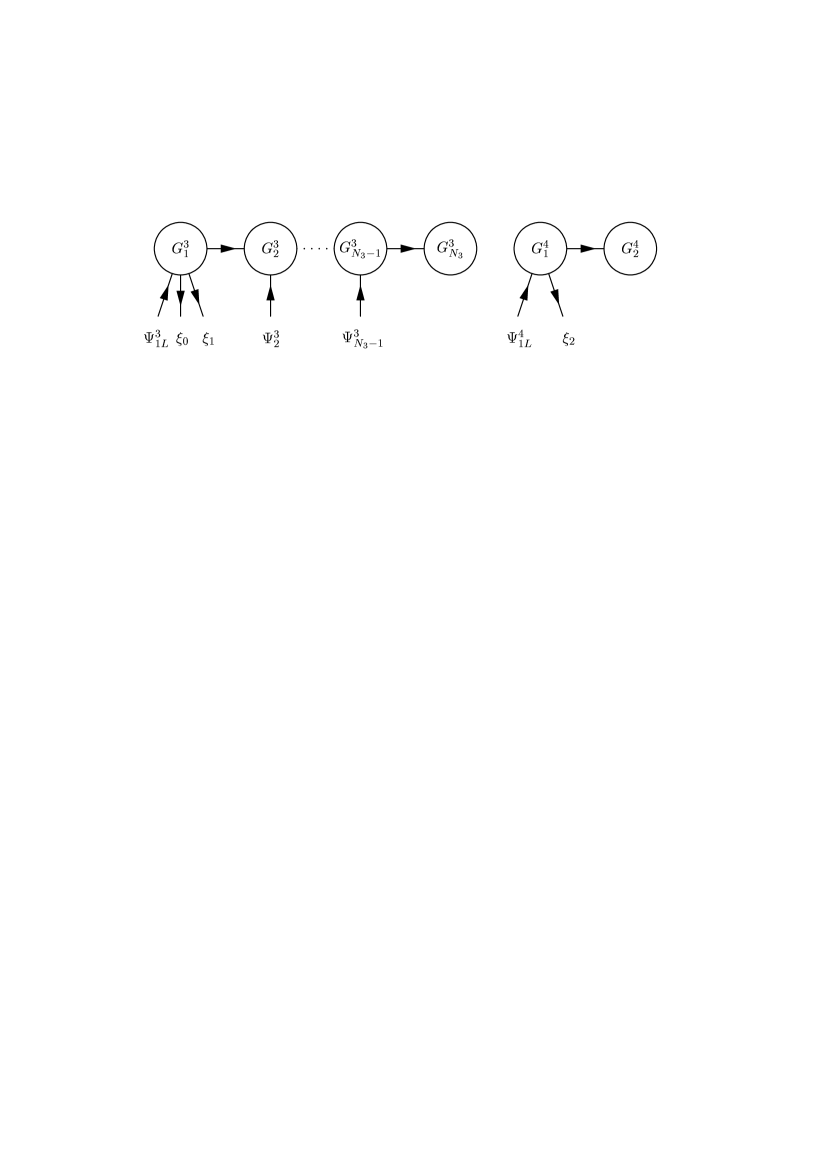
Figure 7: Moose diagram for the location of scalars and chiral fermions in the orbifold extra dimensions associated with the gauge groups $G^{3}$ and $G^{4}$.

Since the charged leptons cannot experience these topologies, the site-fields $\xi_{0},\xi_{1},$ and $\xi_{2}$ are now only relevant for the generation of the neutrino mass matrix and we can discard them in the discussion of the charged lepton mass matrix.

7.2 The one-generation-case

Let us first restrict to the case of one generation by considering the coupling of the $\mathscr{G}$-singlet neutrino $\nu_{e}$ to the fermionic site variables of the orbifold extra dimensions. From table 1 we conclude that $G_{L}\times G_{R}$ gauge-invariance requires the relevant effective Yukawa interaction of the electron lepton doublet $\mathbf{1}_{\ell}$ with the bulk-fermions to be of the type

$${\mathscr{L}}_{2} = Y_{1}\overline{\mathbf{1}^{c}_{\ell}}\tilde{H}^{\ast}\mathbf{1}_{FL}+Y_{2}\overline{\mathbf{1}}_{FR}\xi_{0}\Psi^{3}_{1L}+M_{1F}\overline{\mathbf{1}}_{FR}\mathbf{1}_{FL}+{\rm h.c.},$$ (46)

where $Y_{1}$ and $Y_{2}$ are order unity coefficients, $\tilde{H}$ is the charge-conjugated Higgs-field $\tilde{H}={\rm i}\sigma^{2}H^{\ast}$, and $M_{1F}\simeq 10^{15}\>{\rm GeV}$ denotes the seesaw scale. Suppressing the index $j=3$, the Lagrangian for the bulk and brane fields is given by $\mathscr{L}_{1}+\mathscr{L}_{2}$, where $\mathscr{L}_{1}$ has been defined in Eq. (10). As a result, the $N_{3}\times N_{3}$ mass matrix which emerges from ${\mathscr{L}}_{1}+{\mathscr{L}}_{2}$ after SSB is given by

$$\begin{matrix}&\begin{matrix}\mathbf{1}_{FL}&\Psi_{1L}&\Psi_{2L}&\Psi_{3L}&\cdots\end{matrix}\vspace{1mm}\\ \begin{matrix}\overline{\mathbf{1}^{c}_{\ell}}\\ \overline{\mathbf{1}}_{FR}\\ \overline{\Psi}_{2R}\\ \overline{\Psi}_{3R}\\ \vdots\end{matrix}&\left(\hskip 8.53581pt\begin{matrix}h_{1}&0&0&0&\cdots\\ M_{1F}&h_{2}&0&0&\cdots\\ 0&M_{f}&-M_{f}&0&\cdots\\ 0&0&M_{f}&-M_{f}&\cdots\\ \vdots&\vdots&\vdots&\vdots&\ddots\end{matrix}\hskip 8.53581pt\right)\end{matrix},$$ (47)

where we have introduced the VEVs $h_{1}\equiv Y_{1}\langle\tilde{H}^{\ast}\rangle$, $h_{2}\equiv Y_{2}\langle\xi_{0}\rangle$, and use $h_{1}\simeq h_{2}\simeq 10^{2}\>{\rm GeV}$, i.e., the associated mass terms are generated at the electroweak scale. Note that the mass matrix in Eq. (47) has been displayed in a basis where the active neutrinos have right-handed chirality. Integrating out the heavy $\mathscr{G}$-singlet $\mathbf{1}_{F}$, yields the effective $(N_{3}-1)\times(N_{3}-1)$ mass matrix

$${\mathcal{M}}_{2}\equiv\left(\begin{matrix}m_{\nu}&0&0&\cdots\\ M_{f}&-M_{f}&0&\cdots\\ 0&M_{f}&-M_{f}&\cdots\\ \vdots&\vdots&\vdots&\ddots\\ \end{matrix}\right),$$ (48)

where $m_{\nu}=h_{1}h_{2}/M_{1F}\simeq 10^{-3}\>{\rm eV}$ denotes the absolute neutrino mass scale. The mass $m_{\nu}$ lifts the zero eigenvalue in the KK mass spectrum of the left-handed fields to a small but non-vanishing value which can be determined by diagonalizing the $(N_{3}-1)\times(N_{3}-1)$ matrix

$${\mathcal{M}}_{2}{\mathcal{M}}_{2}^{\dagger}=\left(\begin{matrix}m_{\nu}^{2}&m_{\nu}M_{f}&0&\cdots\\ m_{\nu}M_{f}&2M_{f}^{2}&-M_{f}^{2}&\cdots\\ 0&-M_{f}^{2}&2M_{f}^{2}&\cdots\\ \vdots&\vdots&\vdots&\ddots\end{matrix}\right).$$ (49)

From Eq. (49) it is readily seen that the mixing of $\mathbf{1}^{c}_{\ell}$ with the right-handed fields $\Psi_{nR}$ is described by angles $\simeq m_{\nu}/M_{f}$ which vanish in the limit $M_{f}\rightarrow\infty$. For $m_{\nu}\ll M_{f}$ the non-zero heavy masses are approximately given by the KK spectrum in Eq. (15) where $n=1,\ldots,N_{3}-2$. The lightest eigenvalue $(m_{0})^{2}$ of ${\mathcal{M}}_{2}{\mathcal{M}}_{2}^{\dagger}$ can be determined by integrating out the invertible heavy $(N_{3}-2)\times(N_{3}-2)$ submatrix in the down-right corner of ${\mathcal{M}}_{2}{\mathcal{M}}_{2}^{\dagger}$ in Eq. (49). Taking into account that the $(1,1)$-element of the inverse of this submatrix is equal to $\frac{N_{3}-2}{N_{3}-1}M_{f}^{-2}$, we obtain in the limit $m_{\nu}\ll M_{f}$ for the lightest mass eigenvalue

$$m_{0}=m_{\nu}/\sqrt{N_{3}-1}=m_{\nu}/\sqrt{M_{f}R},$$ (50)

where the second equation matches onto the continuum limit. In the classical 5D continuum theory the mass (or volume) suppression factor $\sim\sqrt{M_{f}R}$ emerges from the normalization of the wave-function of the right-handed neutrino propagating in the bulk [63]. In our deconstruction setup, Eq. (50) states that for a given number of sites there is a non-decoupling of the deconstruction physics from the low-energy theory. Since, as already stated after Eq. (49), the mixing of the active SM lepton $\mathbf{1}^{c}_{\ell}$ with the right-handed fields $\Psi_{nR}$ vanishes in the limit $M_{f}\rightarrow\infty$, we can repeat the above construction for additional aliphatic models which, after integrating out the corresponding KK towers, give rise to further light Dirac neutrino masses. In this way, one can build up a Dirac neutrino mass matrix, which reflects the properties of the dynamically generated extra dimensions.

7.3 Inclusion of the 2nd and 3rd generations

The full neutrino mass matrix emerges by inclusion of the $SU(2)$ lepton doublets of the 2nd and 3rd generation, which are combined into the $\mathscr{G}$-doublet $\mathbf{2}_{\ell}$. Actually, gauge-invariance under $G_{L}\times G_{R}$ allows for the fields $\xi_{2}$ and $\xi_{3}$ Yukawa interactions with $\mathbf{2}_{\ell}$ which read

$${\mathscr{L}}_{3} = Y_{3}\overline{\mathbf{2}^{c}_{\ell}}\tilde{H}^{\ast}\mathbf{2}_{FL}+Y_{4}\overline{\mathbf{2}}_{FR}\xi_{1}\Psi^{3}_{1L}+Y_{5}\overline{\mathbf{2}}_{FR}\xi_{2}\Psi^{4}_{1L}+M_{2F}\overline{\mathbf{2}}_{FR}\mathbf{2}_{FL}+{\rm h.c.},$$ (51)

where $Y_{3},Y_{4},$ and $Y_{5}$ denote order unity Yukawa couplings, $\langle\xi_{1}\rangle\simeq\langle\xi_{2}\rangle\simeq 10^{2}\>{\rm GeV}$, and $M_{2F}\simeq 10^{15}\>{\rm GeV}$. In the construction of Sec. 2.2 we associate with the Weyl spinor $\Psi^{4}_{1L}$ a two-site model for $G^{4}$ where $\Psi^{4}_{1L}$ resides on the site corresponding to $G^{4}_{1}$ (see Fig.7). In complete analogy to the calculation of the light mass $m_{0}$ in Sec. 7.2, one can in the combined system $(\sum_{i=3,4}\mathscr{L}_{1})+{\mathscr{L}}_{2}+{\mathscr{L}}_{3}$, where $\sum_{i=3,4}\mathscr{L}_{1}$ summarizes the aliphatic chains of $G^{3}$ and $G^{4}$, integrate out the heavy vectorlike degrees of freedom. As a consequence, in the basis where the VEVs of $\xi_{1}$ and $\xi_{2}$ are described by Eqs. (34a) and (35a) the resulting $3\times 2$ light Dirac neutrino mass matrix can be written as

$${\mathcal{M}}_{D}=m_{\nu}\left(\begin{matrix}\rho\epsilon&0\\ \epsilon&1\\ -\epsilon&1\end{matrix}\right),$$ (52)

where the neutrino expansion parameter $\epsilon\simeq 1/\sqrt{N_{3}-1}$ and the order unity Yukawa coupling $\rho=\mathcal{O}(1)$ are both real quantities and $m_{\nu}$ denotes the absolute neutrino mass scale. In Eq. (52) all phases have been absorbed into the right-handed neutrino and charged lepton sectors implying the practical absence of $\mathcal{CP}$ violation in neutrino oscillations. The Dirac neutrino mass matrix $\mathcal{M}_{D}$ in Eq. (52) has the important property that within each column the flavor symmetry $\mathscr{G}$ enforces the 2nd and 3rd elements to be relatively real and exactly degenerate in their magnitudes. Thus, $\mathcal{M}_{D}$ describes an exactly maximal $\nu_{\mu}$-$\nu_{\tau}$-mixing. The structure of $\mathcal{M}_{D}$ is familiar from models of single right-handed neutrino dominance [28] which provide an understanding of normal hierarchical neutrino mass spectra in the context of the MSW LMA solution.

7.4 Neutrino masses and mixing angles

The neutrino masses and leptonic mixing angles are determined from Eq. (52) by diagonalizing the matrix

$${\mathcal{M}}_{D}{\mathcal{M}}_{D}^{\dagger}=m_{\nu}^{2}\left(\begin{matrix}\rho^{2}\epsilon^{2}&\rho\epsilon^{2}&-\rho\epsilon^{2}\\ \rho\epsilon^{2}&1+\epsilon^{2}&1-\epsilon^{2}\\ -\rho\epsilon^{2}&1-\epsilon^{2}&1+\epsilon^{2}\end{matrix}\right).$$ (53)

The matrix in Eq. (53) is brought on diagonal form by a rotation of the active neutrino fields in the 2-3-plane through an angle $\theta_{23}=\pi/4$ followed by a rotation in the 1-2-plane through an angle

$$\theta_{12}={\rm arctan}\left[(2\sqrt{2})^{-1}\left(\rho^{2}-2+\sqrt{(2-\rho)^{2}+8}\right)\right].$$ (54)

Hence, the reactor mixing angle $\theta_{13}$ exactly vanishes in agreement with the CHOOZ reactor neutrino data which sets the upper bound $|\theta_{13}|\lesssim 9.2^{\circ}$ [65]. The neutrino masses exhibit the normal hierarchy

$$m_{1}=0,\quad m_{2}=m_{\nu}\epsilon\sqrt{2+\rho^{2}},\quad m_{3}=\sqrt{2}m_{\nu},$$ (55)

which gives for the solar and atmospheric neutrino mass squared differences

$$\Delta m^{2}_{\odot}=m_{\nu}^{2}\epsilon^{2}(2+\rho^{2}),\quad\Delta m^{2}_{\rm atm}=2m_{\nu}^{2}-\Delta m^{2}_{\odot}.$$ (56)

Using the upper bound $\Delta m^{2}_{\odot}\lesssim 1.9\times 10^{-4}\>{\rm eV}^{2}$ [17] and the best-fit value $\Delta m_{\rm atm}^{2}\simeq 2.5\times 10^{-3}\>{\rm eV}^{2}$ [9] we obtain $m_{\nu}\simeq 0.04\>{\rm eV}$ which is consistent with the value $M_{F_{1}}\simeq M_{F_{2}}\simeq 10^{15}\>{\rm GeV}$ for the seesaw scale. Without tuning of parameters we have $\rho=1$ and $\epsilon=1/\sqrt{N_{3}-1}$ which gives for the solar neutrino parameters the values

$$\Delta m^{2}_{\odot}\simeq\frac{3}{2}\frac{\Delta m_{\rm atm}^{2}}{N_{3}-1},\quad\theta_{12}={\rm arctan}\>\frac{1}{\sqrt{2}}\simeq 35^{\circ},$$ (57)

where we have used in the first equation the hierarchy $\Delta m_{\odot}^{2}\ll\Delta m_{\rm atm}^{2}$. At $3\sigma$, the combined solar and KamLAND neutrino data allows for $\Delta m_{\odot}^{2}$ the two regions $5.1\times 10^{-5}\>{\rm eV}^{2}\lesssim\Delta m_{\odot}^{2}\lesssim 9.7\times 10^{-5}\>{\rm eV}^{2}$ (LMA-I) and $1.2\times 10^{-4}\>{\rm eV}^{2}\lesssim\Delta m_{\odot}^{2}\lesssim 1.9\times 10^{-4}\>{\rm eV}^{2}$ (LMA-II) [17]. Matching onto these values requires

$$N_{3}=57\pm 17\quad\text{LMA-I},\qquad N_{3}=27\pm 6\quad\text{LMA-II},$$ (58)

where we have set in Eq. (57) the atmospheric mass squared difference equal to the best-fit value $\Delta m_{\rm atm}^{2}=2.5\times 10^{-3}\>{\rm eV}^{2}$. In short, the presently allowed ratios $\Delta m_{\odot}^{2}/\Delta m_{\rm atm}^{2}$ implied by the LMA-I and LMA-II solutions already significantly discriminate between the associated radii $N_{3}/(2\pi gv)$ of the dynamically generated $\mathcal{S}^{1}/Z_{2}$ orbifold. At this level, the neutrino expansion parameter is $0.12\lesssim\epsilon\lesssim 0.16$ (LMA-I) or $0.18\lesssim\epsilon\lesssim 0.23$ (LMA-II), which is comparable with the Wolfenstein parameter $\lambda\simeq 0.22$ of the charged fermion sector. For the non-fine-tuned solar mixing angle $\theta_{12}={\rm arctan}\>1/\sqrt{2}$ in Eq. (57) we find from the analysis in Ref. [18] that a number of

$$55\pm 8\quad\text{LMA-I}\>\>(@\>90\%\>\text{C.L.})$$ (59)

lattice sites yields the MSW LMA-I solution within the 90% confidence level region. In general, for both the LMA-I and the LMA-II solution, the dynamical generation of the solar mass squared difference $\Delta m_{\odot}^{2}$ via deconstruction in a flat background requires a relatively fine-grained latticization of the associated $\mathcal{S}^{1}/Z_{2}$ orbifold with roughly $10^{1}-10^{2}$ lattice sites.

8 Summary and Conclusions

In conclusion, we have presented a model for lepton masses and mixing angles based on a non-Abelian discrete flavor symmetry and $U(1)$ charges in a deconstructed setup. The model applies the vacuum alignment mechanism of previous models[33, 34] in order to predict an exactly maximal $\nu_{\mu}$-$\nu_{\tau}$-mixing as well as the strict hierarchy $m_{\mu}\ll m_{\tau}$ between the muon and the tau mass. The non-Abelian discrete symmetry is identified as a split extension of the Klein group $Z_{2}\times Z_{2}$ where the lift of every fermion and scalar representation is equivalent with the dihedral group $\mathscr{D}_{4}$ of order eight. The charged lepton masses are generated by the Froggatt-Nielsen mechanism which is given a geometric interpretation in terms of deconstructed or latticized extra dimensions compactified on the circle $\mathcal{S}^{1}$. In theory space, the muon and tau masses correspond to Wilson loops around the plaquettes associated with the deconstructed extra-dimensional $U(1)$ gauge symmetries. As a result, the model gives the realistic charged lepton mass ratios $m_{e}/m_{\tau}\simeq\lambda^{6}$ and $m_{\mu}/m_{\tau}\simeq\lambda^{2}$, where $\lambda\simeq 0.22$ is the Wolfenstein parameter. Since the charged lepton mass matrix is of diagonal form, the leptonic mixing angles stem entirely from the neutrino sector. Enforced by the symmetries, the vacuum structure yields an exactly maximal atmospheric mixing angle $\theta_{23}=\pi/4$ and a vanishing reactor angle $\theta_{13}=0$. In addition, all $\mathcal{CP}$ violation phases vanish due to the symmetries. The model provides an order of magnitude understanding of the solar mixing angle $\theta_{12}$, which is predicted to be large but not necessarily close to maximal. Specifically, without tuning of parameters (i.e., by choosing universal values for all real Yukawa couplings of order unity) the model yields the solar mixing angle $\theta_{12}={\rm arctan}\>1/\sqrt{2}\simeq 35^{\circ}$. The neutrinos exhibit a normal mass hierarchy through single right-handed neutrino dominance which is realized by the propagation of right-handed neutrinos in latticized $\mathcal{S}^{1}/Z_{2}$ orbifold extra dimensions. Here, the solar mass squared difference $\Delta m_{\odot}^{2}$ is suppressed against the atmospheric mass squared difference $\Delta m_{\rm atm}^{2}$ by the discretized analogue of the volume factor, known from the classical theory. For a latticization of the orbifold with $10^{1}-10^{2}$ lattice sites the model yields without tuning of parameters the MSW LMA solution (LMA-I) of the solar neutrino problem within the 90% confidence level region.

Appendix A The dihedral group $\mathscr{D}_{4}$

The dihedral groups $\mathscr{D}_{n}$, where $n=2,3,\ldots$, are the point-symmetry groups with an $n$-fold axis and a system of 2-fold axes at right angle to it. The group $\mathscr{D}_{n}$ is therefore the symmetry group of a regular $n$-gon. These groups contain $2n$ elements and for $n>2$ they are non-Abelian ($\mathscr{D}_{2}$ is isomorphic with the Klein group $Z_{2}\times Z_{2}$). In Fig. 8 the horizontal plane is shown for the case $n=4$, where $a,a^{\prime},b,$ and $b^{\prime}$ denote the four two-fold axes and the 4-fold axis is perpendicular to the paper.

Figure 8: Horizontal plane with the system of two-fold axes for $\mathscr{D}_{4}$.

We denote by $C_{n}$ the operation of rotation through $2\pi/n$ about the principal axis. The $k$-fold application of this transformation will be written as $C_{n}^{k}$ and the identity transformation $C^{n}_{n}$ as $E$. The rotations through $\pi$ about the axes $a,a^{\prime},b,$ and $b^{\prime}$ will be referred to as $C_{a},C_{a^{\prime}},C_{b},$ and $C_{b^{\prime}}$, respectively. Then, the dihedral group ${\mathscr{D}}_{4}$ has eight elements in following five classes:

$$E;\quad C_{4},C_{4}^{3};\quad C_{4}^{2};\quad C_{a},C_{b};\quad C_{a^{\prime}},C_{b^{\prime}}.$$ (60)

Adopting the notation of Ref. [66] we will refer to the five classes which are associated with the sequence in Eq. (60) as $E,C_{4}(2),C_{4}^{2},C_{2}(2),$ and $C_{2^{\prime}}(2)$. Calling the 4 irreducible singlet representations $\mathbf{1_{A}},\mathbf{1_{B}},\mathbf{1_{C}},$ and $\mathbf{1_{D}}$ respectively, the decomposition of the product of the two-dimensional irrep $\mathbf{2}$ reads

$$\mathbf{2}\times\mathbf{2}=\mathbf{1_{A}}+\mathbf{1_{B}}+\mathbf{1_{C}}+\mathbf{1_{D}}.$$ (61)

The character table for the group ${\mathscr{D}}_{4}$ is given in table 5. Denoting $\mathbf{2}$ as $(a,b)$ we have for the singlet representations

$$\mathbf{1_{A}} = a_{1}a_{2}+b_{1}b_{2},$$ (62a)

$$\mathbf{1_{B}} = a_{1}b_{2}-a_{2}b_{1},$$ (62b)

$$\mathbf{1_{C}} = a_{1}a_{2}-b_{1}b_{2},$$ (62c)

$$\mathbf{1_{D}} = a_{1}b_{2}+a_{2}b_{1}.$$ (62d)

From the character table of $\mathscr{D}_{4}$ one determines the decomposition of the product of any two representations as shown in table 6.

$\mathscr{D}_{4}$	$E$	$C_{4}^{2}$	$C_{4}(2)$	$C_{2}(2)$	$C_{2^{\prime}}(2)$
$\mathbf{1_{A}}$	1	1	1	1	1
$\mathbf{1_{B}}$	1	1	1	-1	-1
$\mathbf{1_{C}}$	1	1	-1	1	-1
$\mathbf{1_{D}}$	1	1	-1	-1	1
$\mathbf{2}$	2	-2	0	0	0

Table 5: Character table for the group $\mathscr{D}_{4}$.

$\mathscr{D}_{4}$	$\mathbf{1_{A}}$	$\mathbf{1_{B}}$	$\mathbf{1_{C}}$	$\mathbf{1_{D}}$	$\mathbf{2}$
$\mathbf{1_{A}}$	$\mathbf{1_{A}}$	$\mathbf{1_{B}}$	$\mathbf{1_{C}}$	$\mathbf{1_{D}}$	$\mathbf{2}$
$\mathbf{1_{B}}$		$\mathbf{1_{A}}$	$\mathbf{1_{D}}$	$\mathbf{1_{C}}$	$\mathbf{2}$
$\mathbf{1_{C}}$			$\mathbf{1_{A}}$	$\mathbf{1_{B}}$	$\mathbf{2}$
$\mathbf{1_{D}}$				$\mathbf{1_{A}}$	$\mathbf{2}$

Table 6: Multiplication table for the group $\mathscr{D}_{4}$.

In the vector representation of ${\mathscr{D}}_{4}$, the $2\times 2$ representation matrices corresponding to the different classes can be written as

$$E \quad:\quad D(E)=\left(\begin{matrix}1&0\\ 0&1\end{matrix}\right),$$

$$C_{4}(2) \quad:\quad D(C_{4})=\left(\begin{matrix}0&1\\ -1&0\end{matrix}\right),\quad D(C_{4}^{3})=\left(\begin{matrix}0&-1\\ 1&0\end{matrix}\right),$$

$$C_{4}^{2} \quad:\quad D(C_{4}^{2})=\left(\begin{matrix}-1&0\\ 0&-1\end{matrix}\right),$$

$$C_{2}(2) \quad:\quad D(C_{a})=\left(\begin{matrix}1&0\\ 0&-1\end{matrix}\right),\quad D(C_{b})=\left(\begin{matrix}-1&0\\ 0&1\end{matrix}\right),$$

$$C_{2^{\prime}}(2) \quad:\quad D(C_{a^{\prime}})=\left(\begin{matrix}0&-1\\ -1&0\end{matrix}\right),\quad D(C_{b^{\prime}})=\left(\begin{matrix}0&1\\ 1&0\end{matrix}\right).$$ (63)

Before concluding this section, let us construct the dihedral groups from semi-direct products. For this purpose, let $N\simeq Z_{n}$ for any $n\in\mathbbm{N}$, let $H\simeq Z_{2}$, and let the map $\varphi:H\rightarrow\text{Aut}(N)$ send $h\in H$ to the automorphism in $\text{Aut}(N)$ sending each element of $N$ to its inverse. Then, the external semi-direct product $N\rtimes_{\varphi}H$ of $N$ by $H$ with respect to $\varphi$ is the dihedral group $\mathscr{D}_{n}$. One can also define the infinite dihedral group $\mathscr{D}_{\infty}=N\rtimes_{\varphi}H$, where $N\simeq Z$ and the group $H$ and the map $\varphi$ are as above.

Appendix B Minimization of the tree-level potential

We will rewrite the potential $V_{A}(\Phi,\Omega)$ in Eqs. (5) in terms of the parameterization in Eqs. (31) as follows

$$V_{A} = d_{1}v_{1}^{4}c_{\alpha}^{2}s_{\alpha}^{2}+d_{2}v_{2}^{4}c_{\beta}^{2}s_{\beta}^{2}+d_{3}v_{1}^{2}v_{2}^{2}(c_{\alpha}^{2}-s_{\alpha}^{2})(c_{\beta}^{2}-s_{\beta}^{2}),$$ (64)

where $s_{\alpha}\equiv{\rm sin}(\alpha)$ and $c_{\alpha}\equiv{\rm cos}(\alpha)$ (correspondingly for $\beta$). Hence, it is

$$\frac{\partial V_{A}}{\partial\alpha} = 2d_{1}v_{1}^{4}(c_{\alpha}^{3}s_{\alpha}-c_{\alpha}s_{\alpha}^{3})-4d_{3}v_{1}^{2}v_{2}^{2}c_{\alpha}s_{\alpha}(c_{\beta}^{2}-s_{\beta}^{2}),$$

$$\frac{\partial V_{A}}{\partial\beta} = 2d_{2}v_{2}^{4}(c_{\beta}^{3}s_{\beta}-c_{\beta}s_{\beta}^{3})-4d_{3}v_{1}^{2}v_{2}^{2}c_{\beta}s_{\beta}(c_{\alpha}^{2}-s_{\alpha}^{2}).$$

As a result, at $(\alpha,\beta)=(\frac{\pi}{4},\frac{\pi}{4})$ it is $(\partial_{\alpha},\partial_{\beta})V_{A}=(0,0)$, i.e., $(\alpha,\beta)=(\frac{\pi}{4},\frac{\pi}{4})$ is an extremum of the potential $V_{A}$. For the second derivatives it follows

$$\frac{\partial^{2}V_{A}}{\partial\alpha^{2}} = 2d_{1}v_{1}^{4}(s_{\alpha}^{4}+c_{\alpha}^{4}-6c_{\alpha}^{2}s_{\alpha}^{2})-4d_{3}v_{1}^{2}v_{2}^{2}(c_{\alpha}^{2}-s_{\alpha}^{2})(c_{\beta}^{2}-s_{\beta}^{2}),$$

$$\frac{\partial^{2}V_{A}}{\partial\beta^{2}} = 2d_{2}v_{2}^{4}(s_{\beta}^{4}+c_{\beta}^{4}-6c_{\beta}^{2}s_{\beta}^{2})-4d_{3}v_{1}^{2}v_{2}^{2}(c_{\beta}^{2}-s_{\beta}^{2})(c_{\alpha}^{2}-s_{\alpha}^{2}),$$

$$\frac{\partial^{2}V_{A}}{\partial\alpha\>\partial\beta} = 16d_{3}v_{1}^{2}v_{2}^{2}c_{\alpha}s_{\alpha}c_{\beta}s_{\beta}.$$

At $(\alpha,\beta)=(\frac{\pi}{4},\frac{\pi}{4})$ we therefore obtain for the matrix of second derivatives of the potential

$$\left(\frac{\partial^{2}V_{A}}{\partial\alpha\>\partial\beta}\right)=\left(\begin{matrix}-2d_{1}v_{1}^{4}&4d_{3}v_{1}^{2}v_{2}^{2}\\ 4d_{3}v_{1}^{2}v_{2}^{2}&-2d_{2}v_{2}^{4}\end{matrix}\right),$$ (65)

where, due to the choice $d_{1},d_{2}<0$, the diagonal elements are positive. Hence, if the parameters obey the condition

$$d_{1}d_{2}>4d_{3}^{2},$$ (66)

the matrix in Eq. (65) is positive definite, i.e., the modes which oscillate in the $(\alpha,\beta)$-subspace around $(\alpha,\beta)=(\frac{\pi}{4},\frac{\pi}{4})$ have positive masses and $(\alpha,\beta)=(\frac{\pi}{4},\frac{\pi}{4})$ is a minimum of the scalar potential $V_{A}$. Let us now rewrite the part of the multi-scalar potential $V_{B}(\Phi,\Omega)$ in Eqs. (5) using the parameterization in Eqs. (31) as follows

$$V_{B} = 2d_{4}v_{1}^{4}c_{\alpha}^{2}s_{\alpha}^{2}{\rm cos}(2\varphi)+2d_{5}v_{2}^{4}c_{\beta}^{2}s_{\beta}^{2}\>{\rm cos}(2\psi)$$ (67)

$$+4d_{6}v_{1}^{2}v_{2}^{2}c_{\alpha}s_{\alpha}c_{\beta}s_{\beta}\>{\rm cos}(\varphi)\>{\rm cos}(\psi)$$

$$-4d_{7}v_{1}^{2}v_{2}^{2}c_{\alpha}s_{\alpha}c_{\beta}s_{\beta}\>{\rm sin}(\varphi)\>{\rm sin}(\psi),$$

where we have used the notation of Eq. (64). Hence, one concludes

$$\frac{\partial V_{B}}{\partial\alpha} = 4d_{4}v_{1}^{4}(c_{\alpha}^{3}s_{\alpha}-c_{\alpha}s_{\alpha}^{3})\>{\rm cos}(2\varphi)+4d_{6}v_{1}^{2}v_{2}^{2}(c_{\alpha}^{2}-s_{\alpha}^{2})c_{\beta}s_{\beta}\>{\rm cos}(\varphi)\>{\rm cos}(\psi)$$

$$-4d_{7}v_{1}^{2}v_{2}^{2}(c_{\alpha}^{2}-s_{\alpha}^{2})c_{\beta}s_{\beta}\>{\rm sin}(\varphi)\>{\rm sin}(\psi),$$

$$\frac{\partial V_{B}}{\partial\beta} = 4d_{5}v_{2}^{4}(c_{\beta}^{3}s_{\beta}-c_{\beta}s_{\beta}^{3})\>{\rm cos}(2\psi)+4d_{6}v_{1}^{2}v_{2}^{2}(c_{\beta}^{2}-s_{\beta}^{2})c_{\alpha}s_{\alpha}\>{\rm cos}(\varphi)\>{\rm cos}(\psi)$$

$$-4d_{7}v_{1}^{2}v_{2}^{2}(c_{\beta}^{2}-s_{\beta}^{2})c_{\alpha}s_{\alpha}\>{\rm sin}(\varphi)\>{\rm sin}(\psi),$$

and

$$\frac{\partial V_{B}}{\partial\varphi} = -4d_{4}v_{1}^{4}c_{\alpha}^{2}s_{\alpha}^{2}{\rm sin}(2\varphi)-4d_{6}v_{1}^{2}v_{2}^{2}c_{\alpha}s_{\alpha}c_{\beta}s_{\beta}\>{\rm sin}(\varphi)\>{\rm cos}(\psi)$$

$$-4d_{7}v_{1}^{2}v_{2}^{2}c_{\alpha}s_{\alpha}c_{\beta}s_{\beta}\>{\rm cos}(\varphi)\>{\rm sin}(\psi),$$

$$\frac{\partial V_{B}}{\partial\psi} = -4d_{5}v_{2}^{4}c_{\beta}^{2}s_{\beta}^{2}{\rm sin}(2\psi)-4d_{6}v_{1}^{2}v_{2}^{2}c_{\alpha}s_{\alpha}c_{\beta}s_{\beta}\>{\rm cos}(\varphi)\>{\rm sin}(\psi)$$

$$-4d_{7}v_{1}^{2}v_{2}^{2}c_{\alpha}s_{\alpha}c_{\beta}s_{\beta}\>{\rm sin}(\varphi)\>{\rm cos}(\psi).$$

As a result, at the points $(\alpha,\beta)=(\frac{\pi}{4},\frac{\pi}{4})$, where $\varphi,\psi\in\{0,\pi\}$, it is

$$(\partial_{\alpha},\partial_{\beta},\partial_{\varphi},\partial_{\psi})V_{B}=(0,0,0,0),$$

i.e., these points are extrema of $V_{B}$. Furthermore, one finds at $(\alpha,\beta)=(\frac{\pi}{4},\frac{\pi}{4})$ vanishing mixed second derivatives

$$\frac{\partial^{2}V_{B}}{\partial\varphi\partial\alpha}=\frac{\partial^{2}V_{B}}{\partial\psi\partial\alpha}=\frac{\partial^{2}V_{B}}{\partial\varphi\partial\beta}=\frac{\partial^{2}V_{B}}{\partial\psi\partial\beta}=0,$$

implying that the matrix of the second derivatives of $V_{B}$ with respect to the parameters $\alpha,\beta,\varphi,\psi$ breaks up into a block-diagonal form with submatrices which respectively correspond to the subspaces $(\alpha,\beta)$ and $(\varphi,\psi)$. The second derivatives of $V_{B}$ with respect to $\alpha$ and $\beta$ are

$$\frac{\partial^{2}V_{B}}{\partial\alpha^{2}} = 4d_{4}v_{1}^{4}(s_{\alpha}^{4}+c_{\alpha}^{4}-6c_{\alpha}^{2}s_{\alpha}^{2})\>{\rm cos}(2\varphi)-16d_{6}v_{1}^{2}v_{2}^{2}c_{\alpha}s_{\alpha}c_{\beta}s_{\beta}\>{\rm cos}(\varphi)\>{\rm cos}(\psi)$$

$$+16d_{7}v_{1}^{2}v_{2}^{2}c_{\alpha}s_{\alpha}c_{\beta}s_{\beta}\>{\rm sin}(\varphi)\>{\rm sin}(\psi),$$

$$\frac{\partial^{2}V_{B}}{\partial\beta^{2}} = 4d_{5}v_{2}^{4}(s_{\beta}^{4}+c_{\beta}^{4}-6c_{\beta}^{2}s_{\beta}^{2})\>{\rm cos}(2\psi)-16d_{6}v_{1}^{2}v_{2}^{2}c_{\alpha}s_{\alpha}c_{\beta}s_{\beta}\>{\rm cos}(\varphi)\>{\rm cos}(\psi)$$

$$+16d_{7}v_{1}^{2}v_{2}^{2}c_{\alpha}s_{\alpha}c_{\beta}s_{\beta}\>{\rm sin}(\varphi)\>{\rm sin}(\psi),$$

$$\frac{\partial^{2}V_{B}}{\partial\alpha\partial\beta} = 4d_{6}v_{1}^{2}v_{2}^{2}(c_{\alpha}^{2}-s_{\alpha}^{2})(c_{\beta}^{2}-s_{\beta}^{2})\>{\rm cos}(\varphi)\>{\rm cos}(\psi)$$

$$-4d_{7}v_{1}^{2}v_{2}^{2}(c_{\alpha}^{2}-s_{\alpha}^{2})(c_{\beta}^{2}-s_{\beta}^{2})\>{\rm sin}(\varphi)\>{\rm sin}(\psi).$$

Therefore, at the points $(\alpha,\beta)=(\frac{\pi}{4},\frac{\pi}{4})$, where $\varphi,\psi\in\{0,\pi\}$, the matrix of the second order derivatives is

$$\left(\frac{\partial^{2}V_{B}}{\partial\alpha\>\partial\beta}\right)=4\left(\begin{matrix}-d_{4}v_{1}^{4}-\sigma d_{6}v_{1}^{2}v_{2}^{2}&0\\ 0&-d_{5}v_{2}^{4}-\sigma d_{6}v_{1}^{2}v_{2}^{2}\end{matrix}\right),$$ (68)

where $\sigma\equiv{\rm cos}(\varphi)\>{\rm cos(\psi)}=\pm 1$ can take either sign for $\varphi,\psi\in\{0,\pi\}$. However, from Eq. (67) it is seen that the product $d_{6}\sigma$ must be negative in the lowest energy state, i.e., the sign of $d_{6}$ determines whether $\varphi=\psi+k\cdot 2\pi$ or $\varphi=\psi+k\cdot\pi$ for some integer $k$. The matrix of second order derivatives can therefore be rewritten as

$$\left(\frac{\partial^{2}V_{B}}{\partial\alpha\>\partial\beta}\right)=4\left(\begin{matrix}-d_{4}v_{1}^{4}+|d_{6}|v_{1}^{2}v_{2}^{2}&0\\ 0&-d_{5}v_{2}^{4}+|d_{6}|v_{1}^{2}v_{2}^{2}\end{matrix}\right),$$ (69)

where $d_{4},d_{5}<0$, i.e., the matrix is positive definite. The second derivatives of $V_{B}$ with respect to $\varphi$ and $\psi$ are

$$\frac{\partial^{2}V_{B}}{\partial\varphi^{2}} = -8d_{4}v_{1}^{4}c_{\alpha}^{2}s_{\alpha}^{2}\>{\rm cos}(2\varphi)$$

$$-4d_{6}v_{1}^{2}v_{2}^{2}c_{\alpha}s_{\alpha}c_{\beta}s_{\beta}\>{\rm cos}(\varphi)\>{\rm cos}(\psi)+4d_{7}v_{1}^{2}v_{2}^{2}c_{\alpha}s_{\alpha}c_{\beta}s_{\beta}\>{\rm sin}(\varphi)\>{\rm sin}(\psi),$$

$$\frac{\partial^{2}V_{B}}{\partial\psi^{2}} = -8d_{5}v_{2}^{4}c_{\beta}^{2}s_{\beta}^{2}\>{\rm cos}(2\psi)$$

$$-4d_{6}v_{1}^{2}v_{2}^{2}c_{\alpha}s_{\alpha}c_{\beta}s_{\beta}\>{\rm cos}(\varphi)\>{\rm cos}(\psi)+4d_{7}v_{1}^{2}v_{2}^{2}c_{\alpha}s_{\alpha}c_{\beta}s_{\beta}\>{\rm sin}(\varphi)\>{\rm sin}(\psi),$$

$$\frac{\partial^{2}V_{B}}{\partial\psi\partial\varphi} = 4d_{6}v_{1}^{2}v_{2}^{2}c_{\alpha}s_{\alpha}c_{\beta}s_{\beta}\>{\rm sin}(\varphi)\>{\rm sin}(\psi)-4d_{7}v_{1}^{2}v_{2}^{2}c_{\alpha}s_{\alpha}c_{\beta}s_{\beta}\>{\rm cos}(\varphi)\>{\rm cos}(\psi).$$

At the points $(\alpha,\beta)=(\frac{\pi}{4},\frac{\pi}{4})$, where $\varphi,\psi\in\{0,\pi\}$, the matrix of the second derivatives of $V_{B}$ with respect to $\varphi$ and $\psi$ reads

$$\left(\frac{\partial^{2}V_{B}}{\partial\varphi\partial\psi}\right)=\left(\begin{matrix}-2d_{4}v_{1}^{4}+|d_{6}|v_{1}^{2}v_{2}^{2}&\pm d_{7}v_{1}^{2}v_{2}^{2}\\ \pm d_{7}v_{1}^{2}v_{2}^{2}&-2d_{5}v_{2}^{2}+|\sigma|d_{6}v_{1}^{2}v_{2}^{2}\end{matrix}\right),$$ (70)

where $d_{4},d_{5}<0$, i.e., the diagonal elements are positive. In Eq. (70) we have already used that the potential is minimized when $d_{6}\sigma$ is negative.

Taking everything into account, if the coefficients in the multi-scalar potential satisfy besides Eq. (66) also the condition

$$(-2d_{4}v_{1}^{4}+|d_{6}|v_{1}^{2}v_{2}^{2})(-2d_{5}v_{2}^{4}+|d_{6}|v_{1}^{2}v_{2}^{2})>d_{7}^{2}v_{1}^{4}v_{2}^{4},$$ (71)

then the matrix in Eq. (70) is positive definite, i.e., all modes oscillating in the $(\alpha,\beta,\varphi,\psi)$-subspace around the points $(\alpha,\beta)=(\frac{\pi}{4},\frac{\pi}{4})$, where $\varphi,\psi\in\{0,\pi\}$, have positive masses and hence these points are indeed local minima of both the potentials $V_{A}$ and $V_{B}$, i.e., they locally minimize the term $V_{\Delta}(\Phi,\Omega)$ which breaks the accidental $U(1)^{4}_{\rm acc}$-symmetry.

References

- [1] N. Cabibbo, Phys. Rev. Lett. 10 (1963) 531.
- [2] M. Kobayashi, T. Maskawa, Prog. Theor. Phys. 49 (1973) 652.
- [3] Z. Maki, M. Nakagawa, and S. Sakata, Prog. Theor. Phys. 28 (1962) 870.
-
[4]
C. Wetterich,
Nucl. Phys. B 260 (1985) 402;
C. Wetterich, Nucl. Phys. B 261 (1985) 461;
S. Hamidi and C. Vafa, Nucl. Phys. B 279 (1987) 465;
L. J. Dixon, D. Friedan, E. Martinec, and S. Shenker, Nucl. Phys. B 282 (1987) 13. -
[5]
A. Strominger,
Phys. Rev. Lett. 55 (1985) 2547;
A. Strominger and E. Witten, Commun. Math. Phys. 101 (1985) 341. -
[6]
R. Barbieri, L. J. Hall, and A. Romanino,
Phys. Lett. B 401 (1997) 47;
R. Barbieri, P. Creminelli, and A. Romanino, Nucl. Phys. B 559 (1999) 17;
P. H. Frampton and Adrija Ras̆in, Phys. Lett. B 478 (2000) 424;
Z. Berezhiani and A. Rossi, J. High Energy Phys. 9903 (1999) 002;
T. Blaz̆ek, S. Raby, and K. Tobe, Phys. Rev. D 62 (2000) 055001;
A. Aranda, C. D. Carone, and R. F. Lebed, Phys. Lett. B 474 (2000) 170;
A. Aranda, C. D. Carone, and R. F. Lebed, Phys. Rev. D 62 (2000) 016009. - [7] R. Kuchimanchi and R.N. Mohapatra, Phys. Rev. D 66 (2002) 051301.
-
[8]
Super-Kamiokande Collaboration, Y. Fukuda, et al.,
Phys. Rev. Lett. 81 (1998) 1562;
Super-Kamiokande Collaboration, S. Fukuda, et al., Phys. Rev. Lett. 85 (2000) 3999. - [9] Super-Kamiokande Collaboration, T. Toshito, et al., hep-ex/0105023.
-
[10]
Super-Kamiokande Collaboration, S. Fukuda, et al.,
Phys. Rev. Lett. 86 (2001) 5651;
Super-Kamiokande Collaboration, S. Fukuda, et al., Phys. Lett. B 539 (2002) 179. -
[11]
SNO Collaboration, Q. R. Ahmad , et al.,
Phys. Rev. Lett. 87 (2001) 071301;
SNO Collaboration, Q. R. Ahmad , et al., Phys. Rev. Lett. 89 (2002) 011302. -
[12]
S. P. Mikheyev and A. Y. Smirnov,
Yad. Fiz. 42 (1985) 1441;
S. P. Mikheyev and A. Y. Smirnov, Nuovo Cimento C 9 (1986) 17;
L. Wolfenstein, Phys. Rev. D 17 (1978) 2369. -
[13]
J. N. Bahcall, M. C. Gonzalez-Garcia, C. Peña-Garay,
J. High Energy Phys. 07 (2002) 054;
V. Barger, et al., Phys. Lett. B 537 (2002) 179;
A. Bandyopadhyay, et al., Phys. Lett. B 540 (2002) 14;
P. Aliani, et al., hep-ph/0205053;
P. C. de Holanda and A. Y. Smirnov, hep-ph/0205241. - [14] KamLAND Collaboration, K. Eguchi, et al., hep-ex/0212021.
- [15] V. Barger and D. Marfatia, hep-ph/0212126.
- [16] G. L. Fogli, E. Lisi, D. Montanino, A. Palazzo, and A. M. Rotunno, hep-ph/0212127.
- [17] M. Maltoni, T. Schwetz, and J. W. F. Valle, hep-ph/0212129.
- [18] J. N. Bahcall, M. C. Gonzalez-Garcia, C. Peña-Garay, hep-ph/0212147.
-
[19]
J. K. Elwood, N. Irges, and P. Ramond,
Phys. Rev. Lett 81 (1998) 5064;
N. Irges, S. Lavignac, and P. Ramond, Phys. Rev. D 58 (1998) 035003;
F. S. Ling and P. Ramond, Phys. Lett. B 543 (2002) 29;
Q. Shafi and Z. Tavartkiladze, Phys. Lett. B 459 (1999) 563;
Q. Shafi and Z. Tavartkiladze, Phys. Lett. B 482 (2000) 145;
J. Sato and T. Yanagida, Nucl. Phys. Proc. Suppl. 77 (1999) 293;
G. Altarelli, F. Feruglio, and I. Masina, J. High Energy Phys. 0011 (2000) 040;
N. Maekawa, Prog. Theor. Phys. 106 (2001) 401. -
[20]
Y. Grossman, Y. Nir, and Y. Shadmi,
J. High Energy Phys. 9810 (1998) 007;
M. S. Berger and K. Seyon, Phys. Rev. D 64 (2001) 053006;
G. C. Branco and J. I. Silva-Marcos, Phys. Lett. B 526 (2002) 104. - [21] R. N. Mohapatra and S. Nussinov, Phys. Rev. D 60 (1999) 013002.
- [22] C. Wetterich, Phys. Lett. B 451 (1999) 397.
- [23] S. F. King and G. G. Ross, Phys. Lett. B 520 (2001) 243.
-
[24]
W. Grimus and L. Lavoura,
J. High Energy Phys. 07 (2001) 045;
W. Grimus and L. Lavoura, hep-ph/0211334. - [25] R. N. Mohapatra, A. Pérez-Lorenzana, and C. A. de Sousa Pires, Phys. Lett. B 474 (2000) 355.
- [26] K. S. Babu, E. Ma, and J. W. F. Valle, hep-ph/0206292.
- [27] S. F. King, hep-ph/0208266.
-
[28]
S. F. King,
Nucl. Phys. B 562 (1999) 57;
S. F. King, J. High Energy Phys. 0209 (2002) 11. - [29] N. Arkani-Hamed, A. G. Cohen, and H. Georgi, Phys. Rev. Lett. 86 (2001) 4757.
- [30] C. T. Hill, S. Pokorski, and J. Wang, Phys. Rev. D 64 (2001) 105005.
- [31] C. D. Froggatt and H. B. Nielsen, Nucl. Phys. B 147 (1979) 277.
- [32] C. D. Froggatt, G. Lowe, and H. B. Nielsen, Nucl. Phys. B 420 (1994) 3.
- [33] T. Ohlsson and G. Seidl, Phys. Lett. B 537 (2002) 95.
- [34] T. Ohlsson and G. Seidl, Nucl. Phys. B 643 (2002) 247.
- [35] H. Georgi, Nucl. Phys. B 266 (1986), 274.
- [36] M. R. Douglas and G. Moore, hep-th/9603167.
- [37] N. Arkani-Hamed, A. G. Cohen, and H. Georgi, J. High. Energy Phys. 0207 (2002) 020.
- [38] H. C. Cheng, C. T. Hill, and J. Wang, Phys. Rev. D 64 (2001) 095003.
- [39] A. Falkowski and H. D. Kim, J. High Energy Phys. 0208 (2002) 052.
- [40] L. Randall and R. Sundrum, Phys. Rev. Lett. 83 (1999) 4690.
- [41] W. A. Bardeen and R. B. Pearson, Phys. Rev. D 14 (1976), 547.
- [42] W. A. Bardeen, R. B. Pearson, and E. Rabinovici, Phys. Rev. D 21 (1980) 1037.
- [43] K. G. Wilson, Phys. Rev. D 10 (1974) 2445.
- [44] H. C. Cheng, C. T. Hill, S. Pokorski, and J. Wang, Phys. Rev. D 64 (2001) 065007.
-
[45]
T. Gherghetta and A. Pomarol,
Nucl. Phys. B 586 (2000) 141;
S. J. Huber and Q. Shafi, Phys. Lett. B 498 (2001) 256. - [46] H. Abe, T. Kobayashi, N. Maru, and K. Yoshioka, hep-ph/0205344.
-
[47]
F. Wilczek and A. Zee,
Phys. Rev. Lett. 42 (1979) 421;
S. Weinberg, Phys. Rev. Lett. 43 (1979) 1566. - [48] T. Yanagida, in Proceedings of the Workshop on the Unified Theory and Baryon Number in the Universe, edited by O. Sawada and A. Sugamoto (KEK, Tsukuba, 1979), p. 79.
- [49] M. Gell-Mann, P. Ramond and R. Slansky, Complex Spinors and Unified Theories, in Supergravity, Proceedings of the Workshop on Supergravity, Stony Brook, New York, 1979, edited by P. van Nieuwenhuizen and D.Z. Freedman (North-Holland, Amsterdam, 1979), p. 315.
-
[50]
S. T. Petcov,
Phys. Lett. B 110 (1982) 245;
C. N. Leung and S. T. Petcov, Phys. Lett. B 125 (1983) 461;
R. Barbieri, L. J. Hall, D. Smith, A. Strumia, and N. Weiner, J. High Energy Phys. 9812 (1998) 017. - [51] M. B. Green and J. H. Schwarz, Phys. Lett. B. 149 (1984).
- [52] T. Banks and L. J. Dixon, Nucl. Phys. B 307 (1988) 93.
- [53] R. Barbieri, G. R. Dvali, and A. Strumina, Phys. Lett. B 333 (1994) 79.
- [54] S. M. Barr, Phys. Rev. D 55 (1997) 6775.
- [55] E. Witten, hep-ph/0201018.
- [56] M. Dine, Y. Nir, and Y. Shadmi, hep-ph/0206268.
- [57] M. Creutz, Quarks, Gluons and Lattices (Cambridge University Press, Cambridge, 1983).
-
[58]
E. Witten,
Phys. Lett. B 105 (1981), 267;
M. Leurer, Y. Nir, and N. Seiberg, Nucl. Phys. B 420 (1994) 468. - [59] L. Wolfenstein, Phys. Rev. Lett. 51 (1983) 1945.
- [60] R. Rosenfeld and J. L. Rosner, Phys. Lett. B 516 (2001), 408.
- [61] Particle Data Group, D.E. Groom et al., Eur. Phys. J. C 15 (2000) 1, http://pdg.lbl.gov/.
- [62] Z.-z. Xing, Phys. Lett. B 545 (2002) 352.
-
[63]
K. R. Dienes, E. Dudas, and T. Gherghetta,
Nucl. Phys. B 557 (1999) 25;
N. Arkani-Hamed, S. Dimopoulos, G. Dvali, and J. March-Russel, Phys. Rev. D 65 (2002). - [64] Q. Shafi and Z. Tavartkiladze, hep-ph/0210181.
-
[65]
CHOOZ Collaboration, M. Apollonio, et al.,
Phys. Lett. B 420 (1998) 397;
CHOOZ Collaboration, M. Apollonio, et al., Phys. Lett. B 466 (1999) 415. - [66] M. Hamermesh, Group Theory and Its Application to Physical Problems (Dover, New York, 1989).