Confinement Phenomenology in the Bethe-Salpeter Equation

Abstract

We consider the solution of the Bethe-Salpeter equation in Euclidean metric for a $\bar{q}q$ vector meson in the circumstance where the dressed quark propagators have time-like complex conjugate mass poles. This approximates features encountered in recent QCD modeling via the Dyson-Schwinger equations; the absence of real mass poles simulates quark confinement. The analytic continuation in the total momentum necessary to reach the mass shell for a meson sufficiently heavier than 1 GeV leads to the quark poles being within the integration domain for two variables in the standard approach. Through Feynman integral techniques, we show how the analytic continuation can be implemented in a way suitable for a practical numerical solution. We show that the would-be $\bar{q}q$ width to the meson generated from one quark pole is exactly cancelled by the effect of the conjugate partner pole; the meson mass remains real and there is no spurious $\bar{q}q$ production threshold. The ladder kernel we employ is consistent with one-loop perturbative QCD and has a two-parameter infrared structure found to be successful in recent studies of the light SU(3) meson sector.

I Introduction

QCD models based on the Dyson–Schwinger equations [DSEs] provide an excellent tool in the study of nonperturbative aspects of hadron properties in QCD Roberts and Schmidt (2000). Such models can implement quark and gluon confinement Roberts and Schmidt (2000); Burden et al. (1992); Krein et al. (1992); Maris (1995), generate dynamical chiral symmetry breaking Atkinson and Johnson (1988); Roberts and McKellar (1990), and maintain Poincaré covariance. It is straightforward to implement the correct one-loop renormalization group behavior of QCD Maris and Roberts (1997), and obtain agreement with perturbation theory in the ultraviolet region. Provided that the relevant Ward identities are preserved in the truncation of the DSEs, the corresponding currents are conserved. Axial current conservation induces the Goldstone nature of the pions and kaons Maris et al. (1998); electromagnetic current conservation produces the correct hadronic charge without fine-tuning Oettel et al. (2000).

Previous work Maris and Roberts (1997); Maris and Tandy (1999) has shown this model to provide an efficient description of the light-quark pseudoscalar and vector mesons via two infrared parameters within the rainbow truncation of the DSE for solution of the dressed quark propagators coupled to the ladder approximation for the Bethe-Salpeter equation [BSE]. Furthermore, in impulse approximation, the elastic charge form factors of the pseudoscalars Maris and Tandy (2000) and the electroweak transition form factors of the pseudoscalars and vectors Maris and Tandy (2002); Ji and Maris (2001) are in excellent agreement with data. As a collorary, the strong decays of the vector mesons are well-described in impulse approximation without parameter adjustment Jarecke et al. (2002).

Nonperturbative solutions of the DSEs are almost always implemented in the Euclidean metric for technical reasons and this work is no exception. A resulting complication is that the solution of the BSE for meson bound states requires an analytic continuation in the meson momentum to reach the on-mass-shell point $P^{2}=-M^{2}$. This causes the quark $p^{2}$ in the BSE to vary throughout a domain of the complex plane bounded by a parabola which widens in proportion to the mass $M$ of the meson. For low mass mesons, such as the $\pi$ and $K$ mesons, this excursion into the complex plane is simple to handle. Although the difficulties encountered in studies of ground state vector mesons are greater, they too may be overcome directly Maris and Tandy (1999). For mesons with masses greater than about $1~{}{\rm GeV}$, these excursions into the complex plane are deep enough to encounter singularities in the rainbow DSE solutions for the quark propagators. As a result, little is known about the implementation of the BSE in this situation or even whether a solution is well-defined. For this reason, DSE-BSE model studies of mesons have for the most part been restricted to light mesons. An exception is the study of Ref. Jain and Munczek (1993) in which the Ansatz adopted for the quark propagators in the non-Euclidean domain precluded singular behavior.

It has long been known that the rainbow approximation to the fermion DSE produces complex conjugate singularities on the timelike half of the complex-momentum plane (${\Re}(p^{2})<0$) in QED Fukuda and Kugo (1976); Atkinson and Blatt (1979). The phenomenon has been studied in detail within QED Maris and Holties (1992); Maris (1994) and in an Abelian-like model of QCD Stainsby and Cahill (1992). In these early studies the singularities were attributed to artifacts of the rainbow approximation. A connection between the generation of complex conjugate singularities and the possible absence of real mass poles was noticed in a QED study Fukuda and Kugo (1976). Later studies within QCD Burden et al. (1992); Krein et al. (1992); Gribov (1999) raised suggestions that complex singularities may not be artifacts of the approximation at all, but rather may be a property of the full theory, possibly related to confinement and the absence of real quark mass poles. Beyond the rainbow approximation, very little is known about DSE solutions and their singularity structure. These questions and the influence of approximations have yet to be completely resolved. However they are being addressed; for example, in one simple model calculation, the inclusion of the full dressing of the quark-gluon vertex in the DSE leads to the disappearence of all quark singularities in the complex plane save essential singularities at infinity Burden et al. (1992).

It has been well-established by Dyson-Schwinger studies that in order to obtain an acceptable amount of dynamical chiral symmetry breaking in agreement with empirical observations, the effective rainbow DSE kernel must have a significant infrared strength. This in turn tends to move mass poles away from the real timelike $p^{2}$ axis, at least for a domain characterized by several GeV. This suggests that quark propagators may be successfully modeled in terms of parametrizations based on entire functions Roberts (1996) or at least based on functions with singularities away from the real axis such as complex-conjugate poles.

If such an approach to modeling QCD is to be extended to include $\bar{q}q$ and $\bar{q}Q$ meson spectra beyond 1 or 2 GeV, then it is necessary to determine how solutions of the BSE are defined when complex singularities in the quark propagators may be encountered. This issue is addressed in the following using a simple parmetrization of the quark propagator. Although the method developed herein is first applied to the BSE, it has applications beyond meson spectroscopy. For example, in production processes at moderate momentum transfers, the use of complex mass pole representations for confined quarks has been suggested as a means to handle the sizable timelike momentum carried by the quarks in these processes Ahlig et al. (2001). One deals with these issues also in applications of the DSE-BSE approach to electromagnetic elastic Maris and Tandy (2000) and transition form factors Maris and Tandy (2002); Ji and Maris (2001) of light mesons at high-momentum transfer.

To simplify the analysis, we adopt a parameterization of the dressed quark propagator in terms of complex conjugate mass poles. In the standard approach to the meson BSE, two of the four integration variables are integrated numerically and it is during the integration of these variables that poles may be encountered as a result of analytic continuation. In this article, a clear implementation, based on Feynman integral techniques, is introduced to map the four-dimensional integration in the BSE onto a one-dimensional domain where numerical methods of evaluating Cauchy integrals are well-established. We find that when a complex conjugate mass pole parametrization of the quark propagators is employed, the would-be $\bar{q}q$ decay width of the meson generated from a particular mass pole is exactly cancelled by the contribution of the conjugate partner pole. As a result, the meson mass $M$ remains real valued, even above the pseudo-threshold $M^{2}>\Re(4m_{1}^{2})$ where $m_{1}$ is the lowest complex mass in the propagator representation.

The primary limitation of the method developed here is that it relies on an explicit parameterization of dressed quark propagators in terms of pairs of complex conjugate mass poles. However the limitation is offset by the finding that such a representation can provide excellent fits to both DSE solutions (as is shown in Sec. V) and also to recent lattice-QCD data Detmold (2002). Of course, use of such a phenomenological representation will not exactly preserve the dynamical relation between vertices and propagators necessary to satisfy the Ward Takahashi identities of QCD. In particular, without the axial vector Ward Takahashi identity, the chiral-limit pseudoscalar meson solutions will not obey Goldstone’s theorem Maris et al. (1998). As a result, the toy model introduced in Sec. V would not be recommended for studies of light pseudoscalar mesons; chiral-symmetry-preserving DSE approaches have already been well-established Maris and Roberts (1997); Maris and Tandy (1999) for that sector. Rather, the present work explores techniques for extending the present DSE-based approach to mesons with masses above 1 GeV where one expects to encounter complex conjugate singularities.

The article is organized as follows. In Sec. II, our notation for the ladder BSE for meson states is introduced, as is the complex mass pole representation of the quark propagators which will be employed. In Sec. III, a simplified BSE integral equation is used to illustrate the technique for analytic continuation of the BSE. The fact that the resulting bound state mass will be real is demonstrated explicitly. In Sec. IV, the method is extended to the general BSE for a vector meson. A simple model for the ladder BSE kernel is introduced in Sec. V and numerical results are presented. A discussion of this approach and outlook is presented in Sec. VI.

II The Bethe-Salpeter Equation

In the following the Euclidean metric is employed. The scalar product of two four vectors is then $a\cdot b=\sum_{\mu=1}^{4}a_{\mu}b_{\mu}$, and $a^{2}>0$ for a spacelike 4-vector $a_{\mu}$. The Dirac $\gamma$-matrices are Hermitian $\gamma_{\mu}^{\dagger}=\gamma_{\mu}$ and obey the anti-commutation relation $\{\gamma_{\mu},\gamma_{\nu}\}=2\delta_{\mu\nu}$. The dressed quark propagator $S(p)$ and meson Bethe-Salpeter (BS) amplitude $\Gamma(p;P)$ are solutions of the renormalized DSE,

$$S(p)^{-1}\!\! = \!Z_{2}\,i\,/\!\!\!p+Z_{4}\,m_{q}(\mu)\;$$ (1)

$$+Z_{1}\!\int^{\Lambda}_{q}\!\!\!g^{2}D_{\mu\nu}(p-q)\,\frac{\lambda^{i}}{2}\gamma_{\mu}\,S(q)\,\Gamma^{i}_{\nu}(q,p),$$

and the BSE,

$$\Gamma(p;P)\! = \!\!\int^{\Lambda}_{q}\!\!K(p,q;P)\odot\big{(}S(q_{+})\Gamma(q;P)S(q_{-})\big{)},\;\;$$ (2)

Here $D_{\mu\nu}(k)$ is the renormalized dressed-gluon propagator, $\Gamma^{i}_{\nu}(q,p)$ is the renormalized dressed quark-gluon vertex, $\Gamma(p;P)$ is the BS amplitude for a quark-antiquark bound-state meson, and $K(q,p;P)$ is the renormalized two-particle irreducible $q\bar{q}$ scattering kernel. We consider equal mass quarks with momenta $q_{\pm}=q\pm P/2$ where $q$ is the quark-antiquark relative momentum, and $P=q_{+}-q_{-}$ is the meson momentum which satisfies $P^{2}=-M^{2}$ where $M$ is the meson mass.

In Eq. (2) the double contraction of Dirac indices has been denoted by $\odot$. If the Dirac indices of the elements were reinstated in the BSE and written as parenthetic Roman letters $(a,b,\ldots)$, then Eq. (2) would appear as

$$\Gamma_{(ab)}(p;P)\! = \!\!\int^{\Lambda}_{q}\!\!K_{(ab;cd)}(p,q;P)S_{(de)}(q_{+})$$ (3)

$$\times\Gamma_{(ef)}(q;P)S_{(fc)}(q_{-})~{}~{}.$$

Use of the double contraction operator $\odot$ allows us to suppress Dirac indices, and simplify the forms of the equations appearing herein.

In Eqs. (1) and (2) $\int^{\Lambda}_{k}\equiv\int^{\Lambda}d^{4}k/(2\pi)^{4}$ denotes a translationally invariant ultraviolet regularization of the momentum space integral with mass-scale $\Lambda$. Lorentz covariance entails that the solution of Eq. (1) is of the form $S(p)^{-1}=i/\!\!\!pA(p^{2})+$ $B(p^{2})$. The Lorenz scalars $A(p^{2})$ and $B(p^{2})$ are renormalized at spacelike $p^{2}=\mu^{2}$ such that $A(\mu^{2})=1$ and $B(\mu^{2})=m_{q}(\mu)$, where $m_{q}(\mu)$ is the renormalized current quark mass. After renormalization, one is free to remove the regularization by taking the limit $\Lambda\to\infty$.

Recently, a successful model has been developed that provides an excellent description of the masses, decays and other properties of the light pseudoscalar and vector mesons Maris and Roberts (1997); Maris and Tandy (1999). The model consists of the rainbow-ladder truncations for the quark DSE (1) and meson BSE (2) and the use of an effective $\bar{q}q$ interaction constrained to coincide with perturbative QCD in the ultraviolet domain and containing a phenomenological infrared behavior. In this particular model, the DSE kernel in rainbow truncation is

$$Z_{1}g^{2}D_{\mu\nu}(k)\Gamma^{i}_{\nu}(q,p)\rightarrow 4\pi\alpha_{\rm eff}(k^{2})\,D_{\mu\nu}^{\rm free}(k)\,\gamma_{\nu}\frac{\lambda^{i}}{2}\,,$$ (4)

where $D_{\mu\nu}^{\rm free}(k=p-q)$ is the free gluon propagator in Landau gauge, and $\alpha_{\rm eff}(k^{2})$ is the effective running coupling. The ladder truncation of the BSE kernel is

$$K(p,q;P)\to-4\pi\alpha_{\rm eff}(k^{2})\,D_{\mu\nu}^{\rm free}(k){\frac{\lambda^{i}}{2}}\gamma_{\mu}\otimes{\frac{\lambda^{i}}{2}}\gamma_{\nu}\,,$$ (5)

where $k=p-q$ and $\otimes$ denotes the direct (or Cartesian) product of matrices. This truncation scheme is self-consistent in that it ensures that the dressing of the quark-antiquark vector and axial-vector vertices generated by Eqs. (4) and (5) satisfy their respective Ward-Takahashi identities. This feature is important since the axial-vector Ward-Takahashi identity guarantees that, in the chiral limit of zero current quark mass, the ground state pseudoscalar meson bound states are the massless Goldstone bosons arising from dynamical chiral symmetry breaking in accordance with the Goldstone’s theorem Maris and Roberts (1997); Maris et al. (1998). The vector Ward-Takahashi identity guarantees electromagnetic current conservation for mesons and nucleons if the impulse approximation is used to describe the current in terms of quarks Maris and Tandy (2000); Oettel et al. (2000). The rainbow-ladder truncation is particularly suitable for the flavor octets of light pseudoscalar and vector mesons where higher-order contributions to the quark-gluon skeleton-graph expansion have significant cancellations Bender et al. (1996, 2002) and so may be safely neglected.

With the ladder truncation from Eq. (5), the BSE for a light-quark vector meson is

$$\lambda(P^{2})\Gamma_{\rho}(p;P)=$$

$$\int^{\Lambda}_{q}K^{L}_{\mu\nu}(k)\,\gamma_{\mu}\,S(q_{+})\,\Gamma_{\rho}(q;P)\,S(q_{-})\,\gamma_{\nu}~{},$$

with $k=p-q$ and

$$K^{L}_{\mu\nu}(k)=-\frac{16\pi}{3}\,\alpha_{\rm eff}(k^{2})\,D_{\mu\nu}^{\rm free}(k)~{}.$$ (7)

Here $\Gamma_{\rho}$ is a transverse four vector. We will refer to the vector meson under study here as the $\rho$ meson although, due to a number of simplifications made for illustration purposes, the particular model solutions considered here should not be taken as physical representations of the $\rho$ meson.

A linear eigenvalue $\lambda(P^{2})$ has been introduced into Eq. (LABEL:BSE_ladder) so that it will yield solutions over a continuous range of $P^{2}$. A physical bound state of mass $M_{\rho}$ corresponds to an eigenvalue of $\lambda(P^{2}=-M_{\rho}^{2})=1$. To find such a solution, it is clear that Eq. (LABEL:BSE_ladder) must be analytically continued from Euclidean space where $P^{2}>0$ to Minkowski space where $P^{2}<0$ and the on-mass-shell condition $P^{2}=-M_{\rho}^{2}$ may be realized. In terms of the Euclidean four momentum $P_{\mu}$, such an analytic continuation would correspond to $P_{4}=$ $i\sqrt{\vec{P}^{2}+M_{\rho}^{2}}$, from which it follows that quark momenta $q_{\pm}^{2}=q^{2}$ $-M_{\rho}^{2}/4\pm i\,\sqrt{q^{2}}\,M_{\rho}\,z$ that enter the BSE are complex functions of the integration variables $q^{2}>0$ and the direction cosine $-1\leq z\leq+1$. Therefore, in order to carryout such an analytic continuation of the BSE (LABEL:BSE_ladder), the dressed quark propagators $S(q_{\pm}^{2})$ must be known in the complex-momentum plane within a parabolic region having the negative real (timelike) point $-M_{\rho}^{2}/4$ as the apex and extending symmetrically about the real axis.

Studies within the rainbow-ladder truncation Maris and Tandy (1999) find that the non-analytic points of $u$- and $d$-quark propagators that occur nearest to the origin $q^{2}=0$ are located at $q^{2}=-0.207\pm i0.331~{}{\rm GeV}^{2}$ while those of the $s$-quark propagator are found at $q^{2}=-0.376\pm i0.602~{}{\rm GeV}^{2}$ Jarecke et al. (2002). This finding also agrees with qualitative observations from an earlier study Frank and Roberts (1996). From the positions of these non-analytic points one can define a critical mass $M_{c}=\sqrt{-P^{2}}>0$ above which these singular points enter the domain of integration for the BSE. For the model of LABEL:Maris:1999nt, these critical masses are $M_{c}=1.09$ GeV for $\bar{u}u$ mesons and $M_{c}=1.47$ GeV for $\bar{s}s$ mesons. Clearly, the non-analytic points lie outside the domains of integration for ladder BSE calculations of ground state pseudoscalar and vector mesons, but may lie within the integration domain for heavier mesons. This observation provides one of the main reasons that many BSE studies of mesons focus primarily on light meson states.

The appearence of poles in the domain of integration of the BSE raises two questions: 1) does the analytic continuation of the BSE to timelike momenta $P^{2}<0$ yield physically meaningful quantities, and if so, 2) by what methods does one obtain the solutions of this singular integral equation? The goal of this article is to explore these questions. To facilitate an initial investigation, it is convenient to adopt a parametrization of the quark propagator $S(p)$ as a sum of $N$ pairs of complex conjugate mass poles,

$$S(p)=\sum_{n=1}^{N}\left\{\frac{z_{n}}{i/\!\!\!p+m_{n}}+\frac{z_{n}^{*}}{i/\!\!\!p+m_{n}^{*}}\right\}~{}~{},$$ (8)

where $m_{n}$ are complex-valued mass scales and $z_{n}$ are complex coefficients. Comparison with the general form $S(p)^{-1}=i/\!\!\!pA(p^{2})+$ $B(p^{2})$, allows identification of the amplitudes $A(p^{2})$, $B(p^{2})$, and the quark running-mass $M(p^{2})=B(p^{2})/A(p^{2})$. Equivalently, comparison with the general form $S(p)=-i/\!\!\!p\sigma_{V}(p^{2})+$ $\sigma_{S}(p^{2})$ allows identification of the scalar and vector amplitudes of the propagator, $\sigma_{S}(p^{2})$ and $\sigma_{V}(p^{2})$ respectively. These are needed for the BSE. For example, the quark propagator of Eq. (8) has a scalar amplitude of the form

$$\sigma_{S}(p^{2})=\sum_{n=1}^{N}\left\{\frac{z_{n}\,m_{n}}{p^{2}+m_{n}^{2}}+\frac{z_{n}^{*}\,m_{n}^{*}}{p^{2}+{m_{n}^{*}}^{2}}\right\}~{}~{},$$ (9)

and a vector amplitude $\sigma_{V}(p^{2})$ which is obtained by removing each of the $m_{n}$ and $m_{n}^{*}$ from the numerators.

It is shown in Sec. V that this form of quark propagator with $N=3$ provides an excellent fit to DSE solutions that employ realistic effective $q\bar{q}$ interactions. Furthermore, this form has been used recently to provide a parametric fit of the chiral-quark propagator Detmold (2002) obtained from lattice-QCD simulationsBowman et al. (2002); Bowman (2002).

III Analytic Continuation: A Simple Example

A general study of the analytic continuation of the BSE is quite involved and complicated by the Dirac algebra necessary to describe quark-antiquark states. It is prudent to first proceed by simplifying several of these complications and focus on the issue of analytic continuation of the eigenvalue $\lambda(P^{2})$ and the associated integrations over the complex-conjugate poles in the quark propagator. These restrictions are lifted in Sec. IV where the approach introduced here is extended to the general BSE.

In the following, assume that the quark propagator is well-represented by a single pair of complex conjugate poles (that is, $N=1$ in Eq. (8)). Furthermore, assume that the vector-meson BS amplitude may be represented by the single Dirac amplitude $\Gamma_{\rho}(p;P)=(\delta_{\rho\alpha}-P_{\rho}P_{\alpha}/P^{2})\gamma_{\alpha}\,V(q;P)$, where $P_{\rho}$ is the four momentum of the bound-state vector meson. After these simplifications, the BSE (LABEL:BSE_ladder) may be converted to a scalar eigenvalue equation for the amplitude $V(q;P)$ by multiplication from the left by $\gamma_{\rho}$ followed by a trace over the Dirac indices to obtain

$$\lambda(P^{2})V(p;P)=$$

$$\sum_{a,b=\pm 1}\int^{\Lambda}_{q}\!\!\frac{f_{ab}(p,q,P)\;V(q;P)}{(q_{+}^{2}+\mu^{2}+ia\Delta^{2})\,(q_{-}^{2}+\mu^{2}+ib\Delta^{2})}.~{}~{}$$ (10)

Observe that the kernel of this equation is bilinear in the propagator amplitudes $\sigma_{S}(q_{\pm}^{2})$ and $\sigma_{V}(q_{\pm}^{2})$ but only the denominators of these functions are displayed explicity in Eq. (10). The remaining factors from the quark propagators and effective $q\bar{q}$ interaction have been collected into the scalar function $f_{ab}$ whose detailed form is unimportant to the present discussion but may be derived following the discussion of Sec. IV. In addition, the denominators have been written in terms of $\mu^{2}=m_{R}^{2}-m_{I}^{2}$ and $\Delta^{2}=2m_{R}m_{I}$, where $m=m_{R}+im_{I}$ is the complex mass scale parameter in the quark propagator in Eq. (9). This form allows a parametrization of the square of the quark mass $m^{2}$ and its complex conjugate $m^{2*}$ in terms of the values $a=\pm 1$.

In principle, the $q$-dependence of the integrand in Eq. (10) is only known once the solution $V(q;P)$ has been obtained. For the present, consider the artificial situation in which the solution of the BSE is known to be of the form $V=g\,\phi(q^{2})\;U(z_{q})$ where $z_{q}=q\cdot P/\sqrt{q^{2}P^{2}}$ and $\phi(q^{2})$ and $U(z)$ are known functions. In this case, the constant $g$ may be eliminated from the BSE and following an integration over $d^{4}p$ one obtains,

$$\lambda(P^{2})=\sum_{a,b=\pm 1}\;\lambda_{ab}(P^{2}),$$ (11)

and

$$\lambda_{ab}(P^{2})=\int\!\!\!\frac{d^{4}q}{(2\pi)^{4}}\frac{F_{ab}(q,P)}{(q_{+}^{2}+\mu^{2}+ia\Delta^{2})\,(q_{-}^{2}+\mu^{2}+ib\Delta^{2})}~{}~{},$$ (12)

where $F_{ab}(q,P)$ is a non-singular, Lorentz invariant function of $q$ and $P$. The objective is then to evaluate the four integrals $\lambda_{ab}(P^{2})$ and show how they may be analytical continued to negative values of $P^{2}$. This is carried out explicitly in the remainder of this section.

When $P^{2}$ is continued to negative values, the quark momenta in Eq. (12) satisfy $q_{\pm}^{2}=(q_{\mp}^{2})^{*}$. The two factors in the denominator of $\lambda_{a,-a}(P^{2})$ (that is, $a=-b$ in Eq. (12)) will thus be complex conjugates. As a result, for $P^{2}$ sufficiently timelike, there will always be some value of the integration variable $q_{\mu}$ for which both factors in the denominator of $\lambda_{a,-a}(P^{2})$ vanish simultaneously. The result is a non-analytic point in $\lambda_{+-}(P^{2})$ and $\lambda_{-+}(P^{2})$. Such behavior would usually be indentified with the decay threshold for the vector meson into an asymptotically-free quark and antiquark pair. However, in the following, it is shown that when the integrals in Eq. (12) are added together the imaginary parts cancel exactly thereby eliminating the possibility of quark-antiquark production thresholds. In contrast to this, the two factors in the denominator of $\lambda_{aa}(P^{2})$ never vanish simultaneously and consequently there are no corresponding non-analytic points in either $\lambda_{++}(P^{2})$ or $\lambda_{--}(P^{2})$.

To analyze the behavior in detail, it is advantageous to restructure the integral in Eq. (12) so that the analytic continuation from the Euclidean domain $P^{2}>0$ to the timelike domain $P^{2}<0$ is straightforward. For values of $P^{2}>0$, one may combine the two factors in the denominator using the Feynman parametrization,

$$\frac{1}{AB}=\int_{0}^{1}\!d\alpha d\beta\;\frac{\delta(\alpha+\beta-1)}{(\alpha A+\beta B)^{2}}$$ (13)

and obtain

$$\lambda_{ab}(P^{2})\!\! = \!\!\!\int_{-1}^{+1}\!\!\frac{dy}{2}\int\!\!\!\frac{d^{4}q}{(2\pi)^{4}}\;\frac{F_{ab}(q,P)}{D(q,P,y)^{2}}~{},$$ (14)

where $y=\alpha-\beta$, and

$$D(q,P,y)=y(q\cdot P+i\frac{a\!-\!b}{2}\Delta^{2})+(q^{2}+\frac{P^{2}}{4}+\mu^{2}+i\frac{a\!+\!b}{2}\Delta^{2})~{}.$$ (15)

One then eliminates the term linear in $q$ in the denominator by a shift of the origin $q_{\nu}\rightarrow q_{\nu}-yP_{\nu}/2$. The resulting denominator depends on $P^{2}$, $q^{2}$, and $y$ but not on $q\cdot P$. After this shift, the function $F_{ab}(q,P)$ in the numerator still depends $q\cdot P$. All other variables save $q^{2}$ and $y$ can be integrated out yielding,

$$\lambda_{ab}(P^{2}) = \!\!\int_{-1}^{+1}\!\!\!dy\,\int_{0}^{\infty}\!\!\!dq^{2}\;\frac{q^{2}\,\tilde{F}_{ab}(q^{2},y;P^{2})}{[q^{2}-q^{2}_{ab}(P^{2},y)]^{2}},$$ (16)

where

$$q^{2}_{ab}(P^{2},y)=-\frac{P^{2}}{4}(1-y^{2})-\mu^{2}-\frac{i}{2}\left(y(a-b)+a+b\right)\Delta^{2},$$ (17)

is independent of $q^{2}$, and

$$\tilde{F}_{ab}(q^{2},y;P^{2})\!=\!\frac{1}{16\pi^{3}}\!\int_{-1}^{+1}\!\!\!\!dz_{q}\,\sqrt{1-z_{q}^{2}}\;F_{ab}(q-\frac{y}{2}P,P)~{}.$$ (18)

Here $z_{q}$ is the direction cosine defined by $q\cdot P=\sqrt{q^{2}P^{2}}\,z_{q}$. The singular behavior due to the propagators is now a single second-order pole in the variable $q^{2}$. Its location $q^{2}_{ab}(P^{2},y)$ is given in Eq. (17) and is not in the path of integration for spacelike $P^{2}>0$; the integral is regular in Euclidean space.

Figure 1: The trajectory of pole position $q^{2}_{+-}(y)$ given by Eq. (17) is shown as the dashed curve. The solid curve is the contour required to implement analytic continuation.

The $y$ integration is performed after the integration over $q^{2}$. Hence, for a given value of $y$, the $q^{2}$-integration domain is the positive real axis and the integrand has a pole in the complex $q^{2}$ plane whose location $q^{2}_{ab}(P^{2},y)$ moves with $P^{2}$. The location has a negative real part for $P^{2}>0$ and remains negative as $P^{2}$ passes through zero and becomes moderately timelike. Only when $P^{2}<-4\mu^{2}$ will the real part of the pole location become positive and have a chance of impinging upon the domain of the $q^{2}$-integration. For that to happen, the imaginary part of $q^{2}_{ab}(y)$ would have to vanish. As anticipated above, Eq. (17) shows that this never happens when $a=b$; for $\lambda_{++}(P^{2})$ and $\lambda_{--}(P^{2})$ the two factors in the denominator of Eq. (12) are never zero simultaneously. It is therefore trivial to carryout these integrations. However, for $a=-b$, the imaginary part of $q^{2}_{ab}(y)$ can become zero when the Feynman variable $y=0$ and care must be taken to properly handle such singular integrals.

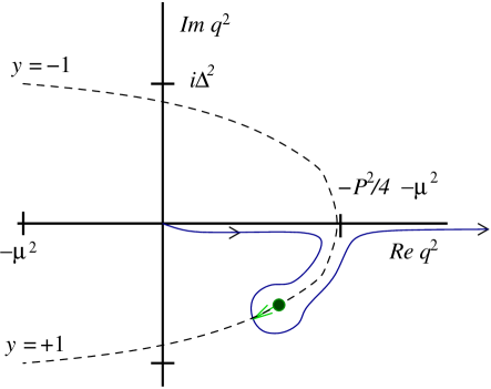
As a specific example, the trajectory of the pole location $q^{2}_{+-}(y)$ is shown in Fig. 1. It begins at $(-\mu^{2},\Delta^{2})$ when $y=-1$, moves along the dashed curve as $y$ increases, crossing the real axis when $y=0$, and terminates at $(-\mu^{2},-\Delta^{2})$ when $y=1$. For $y<0$, the calculation of the integral is straightforward. However for $y>0$, the pole in $q^{2}$ has crossed the real axis and the analytic continuation of the integral $\lambda_{+-}(P^{2})$ is defined by continuous deformation of the contour in a manner that ensures the pole does not cross the contour of integration. This is illustrated in Fig. 1, for the deformed contour corresponding to $y\approx+1/2$. Deformation of a integration contour in this manner is equivalent to adding the pole residue to the result of integration along the real $q^{2}$ axis. If the residue term were neglected, one would obtain a discontinuous result due to the crossing of a branch cut onto the wrong sheet.

For the integral $\lambda_{-+}(P^{2})$, the pole trajectory traces out the same path as in Fig. 1 but in the opposite direction; that is, $y>0$ corresponds to the upper half $q^{2}$-plane and the pole residue will be of opposite sign from $\lambda_{+-}(P^{2})$. After analytic continuation to $P^{2}<0$, the results for the four integrals can be expressed as

$$\lambda_{ab}(P^{2})= \int_{-1}^{+1}\!\!dy\,\int_{0}^{\infty}\!\!ds\frac{s\,\tilde{F}_{ab}(s,y;P^{2})}{[s-q^{2}_{ab}(y,P^{2})]^{2}}$$ (19)

$$+\frac{a-b}{2}\;2\pi i\;\Theta(-\frac{P^{2}}{4}-\mu^{2})$$

$$\times\int_{0}^{1}\!\!dy\frac{d}{ds}\big{(}s\;\tilde{F}_{ab}(s,y;P^{2})\big{)}\bigg{|}_{s=q^{2}_{ab}}~{},$$

where $\Theta(x)$ is the Heaviside step function.

In the timelike region, inspection of Eq. (19) shows that individual integrals $\lambda_{ab}(P^{2})$ are complex valued and satisfy

$$[\lambda_{a,b}(P^{2})]^{*} = \lambda_{-a,-b}(P^{2})~{}.$$ (20)

The imaginary parts cancel in pairs thereby producing a real result for the eigenvalue $\lambda(P^{2})=\sum_{a,b=\pm}\lambda_{ab}(P^{2})$. Notice that this does not mean that one may neglect the addition of residue terms required by the analytic continuation of the integrals. Rather, when $\Delta^{2}>0$ the residue (second) term of Eq. (19) is not purely imaginary and the sum of the real parts of the residues are required for the final result for $\lambda(P^{2})$. Of course, these residue terms appear only for $P^{2}$ more timelike than the pseudo-threshold point $P^{2}=-4\mu^{2}$, that is, for bound state masses $M_{\rho}>2\mu$.

Before extension of this treatment to the general problem, consider the connection between the above discussion of analytic continuation and the usual case encountered above physical two-body thresholds. In particular, consider the limiting case of infinitesimal $\Delta$ for the single integral $\lambda_{--}(P^{2})$. This corresponds to the standard case of employing elementary propagators with the conventional boundary conditions of a negative infinitesimal $-i\epsilon$ added to the real mass. Above the two-body threshold $P^{2}<-4\mu^{2}$, there would be $\bar{q}q$ production described by the residue term in $\lambda_{--}(P^{2})$. It follows that a bound state calculation, based on such an integral alone, would result in a complex mass describing an unstable meson with a finite $\bar{q}q$ decay width. However, in the present case the presence of conjugate quark poles ensures that the analytic continuation introduces both positive and negative would-be widths that cancel exactly. The resulting BSE eigenvalue $\lambda(P^{2})$ in Eq. (10) will be purely real and therefore bound state masses defined by $\lambda(P^{2}=-M_{\rho}^{2})=1$ will be real and will describe a meson with no $\bar{q}q$ decay width.

IV Generalization to the Bethe-Salpeter Equation

The technique described in the previous section is generalized to allow solutions to the homogeneous BSE for an arbitrary quark-antiquark bound state. To be specific, we consider an equal quark-antiquark vector meson bound state. One can write the most-general BS amplitude for a massive vector meson as a sum of eight Dirac covariants and Lorentz-scalar amplitudes $F_{\alpha}(q;P)$,

$$\Gamma_{\rho}(q;P) = \left(\delta_{\rho\mu}-\frac{P_{\rho}P_{\mu}}{P^{2}}\right)\big{(}\gamma_{\mu}\,F_{1}+q_{\mu}\not\!q\,F_{2}$$ (21)

$${}+q_{\mu}\not\!P\,F_{3}+\gamma_{5}\epsilon_{\mu\alpha\nu\beta}\gamma_{\alpha}q_{\nu}P_{\beta}\,F_{4}$$

$${}+q_{\mu}\,F_{5}+\sigma_{\mu\nu}q_{\nu}\,F_{6}+\sigma_{\mu\nu}P_{\nu}\,F_{7}$$

$${}+q_{\mu}\sigma_{\alpha\beta}q_{\alpha}P_{\beta}\,F_{8}\;\big{)}.$$

In a more concise form this is

$$\Gamma_{\rho}(q;P)=\sum_{\alpha=1}^{8}\;\Lambda^{\alpha}_{\rho}(q,P)\,F_{\alpha}(q;P)~{},$$ (22)

where $\Lambda^{\alpha}$ are the Dirac covariants in Eq. (21); for example, $\Lambda^{\alpha=1}_{\rho}=$ $(\delta_{\rho\mu}-P_{\rho}P_{\mu}/P^{2})\,\gamma_{\mu}$. When all indices of a product of two Dirac covariants are contracted in the manner corresponding to the usual trace operation, one obtains

$${\rm tr}_{\rm D}\left[\Lambda_{\mu}^{\alpha}(q,P)\;\Lambda_{\mu}^{\beta}(q,P)\right] = \Lambda_{\mu}^{\alpha}(q,P)\odot\Lambda_{\mu}^{\beta}(q,P),$$ (23)

$$= t_{\alpha\beta}(q,P),$$

where $t_{\beta\alpha}(q,P)$ is a Lorentz scalar function of $q^{2}$, $P^{2}$ and $q\cdot P$, and we have used the double-contraction product $\odot$ notation introduced in Eq. (2).

Of course, one is free to choose any other set of Dirac covariants $\Lambda^{\alpha}_{\rho}(q,P)$ as long as they are complete. In particular, one is free to choose a set of covariants for which $t_{\alpha\beta}\to\delta_{\alpha\beta}$ in which case the resulting set of coupled integral equations may be of a simpler form than those obtained herein. However, in practice the behavior of such covariants can be poorly behaved near $q=0$, and can lead to numerical difficulties Maris and Tandy (1999). Therefore, the set of covariants given by Eq. (21) is preferable and the lack of orthogonality is easily accommodated by $t_{\alpha\beta}(q,P)$.

In the previous section, it was shown that when the $q^{2}$ and $q\cdot P$ dependence of the BS amplitude $\Gamma_{\mu}(q;P)$ is known, the analytic continuation of the BSE may be carried out in a straight-forward manner. In practice, the functional form of the BS amplitude is known only after the solution to the BSE has been obtained. The approach outlined in the previous section may be generalized by expansion of the functional dependence of the BS amplitudes $F_{\alpha}(q;P)$ in terms of complete sets of known functions of $q^{2}$ and $z_{q}={q}\cdot{P}/\sqrt{q^{2}P^{2}}$. Consider the expansion

$$F_{\alpha}(q;P)=\sum_{s,i=0}^{\infty}\,U_{i}(z_{q})\,\phi_{s}(q^{2})\,g^{\alpha}_{si}(P^{2})~{},$$ (24)

where $U_{i}(z_{q})$ are Chebyshev polynomials of the second kind satisfying the ortho-normality condition

$$\frac{2}{\pi}\int_{-1}^{1}\,dz\,\sqrt{1-z^{2}}\,U_{i}(z)\,U_{j}(z)=\delta_{ij}~{},$$ (25)

and $\phi_{s}(q^{2})$ are a set of ortho-normal functions, that are specified later, and that satisfy

$$\int_{0}^{\infty}\!\!\!dq^{2}\;\phi_{s}(q^{2})\;\phi_{t}(q^{2})=\delta_{st}~{}.$$ (26)

The required number of basis terms will be determined by convergence of the BSE solution with respect to the meson observables of interest. For example, one particular choice of basis $\{\phi_{s}(q^{2})\}$ which proves to be efficient for observables dominated by infrared physics may be inefficient for observables sensitive to the ultraviolet. In the present work, we take convergence of the meson mass as the criterion.

For brevity, we define the operator ${\cal O}_{si}(p)$ which projects out the expansion coefficients $g^{\alpha}_{si}(P^{2})$ from the BS amplitude in Eq. (24). Using Eqs. (22) and (23), one finds

$$g^{\alpha}_{si}(P^{2})\! = \!{\cal O}_{si}(p)\;t^{-1}_{\alpha\alpha^{\prime}}(p,P)\Lambda^{\alpha^{\prime}}_{\rho}\odot\Gamma_{\rho}(p;P)$$ (27)

$$= \!\!\int_{0}^{\infty}\!\!\!\!dp^{2}\!\int_{-1}^{+1}\!\!\!\!dz_{p}\sqrt{1-z_{p}^{2}}\;U_{i}(z_{p})\,\phi_{s}(p^{2})$$

$$\times t^{-1}_{\alpha\alpha^{\prime}}(p,P)\,{\rm tr}_{\rm D}\left[\Lambda_{\rho}^{\alpha^{\prime}}(p,P)\;\Gamma_{\rho}(p;P)\right].$$

The set of coefficients $g^{\alpha}_{si}(P^{2})$ will be refered to as BS amplitudes since they are equivalent to the BS amplitude $\Gamma_{\rho}(p;P)$ in that they contain all the dynamical information regarding the solution of the BSE. The expansion coefficients $g^{\alpha}_{si}(P^{2})$ are functions of $P^{2}$ only. The operator ${\cal O}_{si}(p)$ is an integral operator that is introduced for brevity and notational convenience.

When both sides of the BSE (LABEL:BSE_ladder) are projected according to Eq. (27) one obtains

$$\lambda(P^{2})g^{\alpha}_{si} = {\cal O}_{si}(p)\!\!\int\!\!\!\frac{d^{4}q}{(2\pi)^{4}}t^{-1}_{\alpha\alpha^{\prime}}(p,P)\bigg{[}\Lambda_{\rho}^{\alpha^{\prime}}(p)$$ (28)

$$\odot K(p,q;P)\odot\big{(}S(q_{+})\Gamma_{\rho}(q;P)S(q_{-})\big{)}\bigg{]},$$

$$= \!\!\!\sum_{AB\beta tj}\!{\cal O}_{si}(p)\int\!\!\!\frac{d^{4}q}{(2\pi)^{4}}t^{-1}_{\alpha\alpha^{\prime}}(p,P)\bigg{[}\Lambda_{\rho}^{\alpha^{\prime}}(p)$$

$$\!\!\!\odot K(p,q;P)\odot\big{(}\widetilde{\Lambda}^{A}(q_{+})\Lambda_{\rho}^{\beta}(q;P)\widetilde{\Lambda}^{B}(q_{-})\big{)}\bigg{]}$$

$$\times\sigma_{A}(q^{2}_{+})\sigma_{B}(q_{-}^{2})\phi_{t}(q^{2})U_{j}(z_{q})g^{\beta}_{tj},$$

where the sums are over $\beta\in\{1,\ldots,8\}$, and $t,j\in\{0,1,\ldots\}$, and $A,B\in\{V,S\}$. The second equality follows by expanding the BS amplitude $\Gamma_{\rho}(q;P)$ according to Eqs. (22) and (24). In Eq. (28) another set of Dirac covariants, $\widetilde{\Lambda}^{A}(q)=\{-i\gamma\!\cdot\!q,\;1\}$ with $A=V,S$, have been introduced to allow the propagator representation $S(q)=\sum_{A=V,S}\widetilde{\Lambda}^{A}(q)\sigma_{A}(q^{2})$.

At this point, it is helpful to specify a coordinate system. We take $P_{\mu}=$ $\sqrt{P^{2}}(0,0,0,1)$, $p_{\mu}=$ $\sqrt{p^{2}}(0,0,\sqrt{1-z_{p}^{2}},z_{p})$, and the integration momentum $q_{\mu}$ is represented as

$$q_{\mu}=\sqrt{q^{2}}\left(\begin{array}[]{c}\cos\phi\sqrt{1-x_{q}^{2}}\sqrt{1-z_{q}^{2}}\\ \sin\phi\sqrt{1-x_{q}^{2}}\sqrt{1-z_{q}^{2}}\\ x_{q}\sqrt{1-z_{q}^{2}}\\ z_{q}\end{array}\right)~{}.$$ (29)

The integrand in Eq. (28) has no dependence upon angle $\phi$; the only dependence on direction cosine $x_{q}$ is through the $p\cdot q$ dependence of the BS kernel $K(p,q;P)$. In Eq. (28) we may therefore substitute

$$\int d^{4}q=\pi\int_{0}^{\infty}dq^{2}\,q^{2}\int_{-1}^{1}dz_{q}\,\sqrt{1-z_{q}^{2}}\,\int_{-1}^{1}\!\!\!dx_{q}~{}~{}.$$ (30)

The integration over $x_{q}$ in Eq. (28) produces a function of $p^{2},q^{2},z_{p},z_{q}$ and $P^{2}$ which can be expanded in the basis functions. That is, we define a quantity ${\cal V}$ by

$$\int_{-1}^{+1}\!\!\!dx_{q}\;\;t^{-1}_{\alpha\alpha^{\prime}}(p,P)\;\bigg{[}\Lambda^{\alpha^{\prime}}_{\rho}(p)\odot K(p,q;P)$$ (31)

$$\odot\big{(}\widetilde{\Lambda}^{A}(q_{+})\Lambda_{\rho}^{\beta}(q;P)\widetilde{\Lambda}^{B}(q_{-})\big{)}\bigg{]}$$

$$= \sum_{stij}\phi_{s}(p^{2})U_{i}(z_{p})\;{\cal V}^{\alpha A;\beta B}_{si;tj}(P^{2})\;\phi_{t}(q^{2})U_{j}(z_{q})~{}.$$

Upon substituting this back into Eq. (28) above, one obtains a discretized form of the BSE,

$$\lambda(P^{2})\;g_{si}^{\alpha}(P^{2})={\cal V}^{\alpha A;\beta B}_{si;w\ell}(P^{2})\;{\cal G}^{AB}_{w\ell,tj}(P^{2})\;g_{tj}^{\beta}(P^{2})~{},$$ (32)

where repeated indices are understood as being summed over. Here we have introduced the projection of the product of propagator amplitudes in the form

$${\cal G}^{AB}_{si,tj}(P^{2})\! = \!\frac{\pi}{(2\pi)^{4}}\!\int_{0}^{\infty}\!\!\!\!\!dq^{2}q^{2}\!\int_{-1}^{1}\!\!\!dz_{q}\,\sqrt{1-z_{q}^{2}}\phi_{s}(q^{2})U_{i}(z_{q})$$ (33)

$$\times\sigma_{A}(q_{+}^{2})\sigma_{B}(q_{-}^{2})\;\phi_{t}(q^{2})U_{j}(z_{q})~{}.$$

Thus far, the BSE has been reduced to the discrete eigenvalue problem given in Eq. (32). Physical solutions are at $\lambda(P^{2}=-M_{\rho}^{2})=1$ from which one identifies the existence of a bound state vector meson of mass $M_{\rho}$. The only task remaining is the determination of the elements in Eq. (32) that make up the kernel of the eigenvalue problem. These are ${\cal V}$ and ${\cal G}$. The generalized interaction ${\cal V}$ is determined in terms of the kernel by the projection in Eq. (31).

Consider the explicit form of ${\cal G}$. Clearly there is a strong similarity between the form of Eq. (33) and the simple integral whose analytic continuation was considered in Sec. III. This is clarified by the expansion of the quark propagator amplitudes in terms of the mass pole terms from Eq. (9) in the form

$$\sigma_{A}(q^{2})=\sum_{n=1}^{N}\;\sum_{a=\pm 1}\;\frac{Z_{n}^{Aa}}{q^{2}+\mu_{n}^{2}+ia\,\Delta_{n}^{2}}~{},$$ (34)

where $Z^{A\;a=+1}_{n}=z_{n}$ or $z_{n}m_{n}$ for $A=V$ or $S$, respectively, and $Z^{A\;a=-1}_{n}=z_{n}^{*}$ or $z_{n}^{*}m_{n}^{*}$, respectively. Then, Eq. (33) can be written as

$${\cal G}^{AB}_{st;ij}(P^{2})=\frac{1}{2}\sum_{n,m=1}^{N}\sum_{a,b=\pm 1}\;Z_{n}^{Aa}Z_{m}^{Bb}$$

$$\int\!\!\frac{d^{4}q}{(2\pi)^{4}}\;\frac{\phi_{s}(q^{2})U_{i}(z_{q})\,\phi_{t}(q^{2})U_{j}(z_{q})}{(q_{-}^{2}+\mu_{n}^{2}+ia\Delta^{2}_{n})(q_{+}^{2}+\mu_{m}^{2}+ib\Delta^{2}_{m})}.~{}{}$$ (35)

These integrals in Eq. (35) are of the type $\lambda_{ab}(P^{2})$ already explored in our discussion of analytic continuation in Sec. III. The only difference is that the number of integrals that have to be performed can be large since it depends on the number of basis terms for representation of the BS amplitudes via Eq. (24), and the number of conjugate pairs of mass poles for representation of the propagators.

The same methods employed in Sec. III may be used here to calculate the integrals ${\cal G}^{AB}_{st;ij}(P^{2})$ for all values of $P^{2}$ while accounting properly for the analytic continuation. In particular, the Feynman integral method used here will lead to a denominator $[q^{2}-q^{2}_{nmab}(P^{2},y)]^{2}$, where the pole location is

$${q}_{nmab}^{2}(y) = -\frac{P^{2}}{4}(1-y^{2})+y\frac{\mu^{2}_{n}-\mu^{2}_{m}}{2}+\frac{\mu^{2}_{n}+\mu^{2}_{m}}{2}$$ (36)

$$+iy\frac{a\Delta^{2}_{n}-b\Delta^{2}_{m}}{2}+i\frac{a\Delta^{2}_{n}+b\Delta^{2}_{m}}{2}~{}.$$

The integration over $q^{2}$ is carried out first, followed by the integration over the Feynman parameter $y$, and finally the integration over $z_{q}$. Integrations over the two remaining angles in Eq. (35) are trivial. In general, for a quark propagator parametrized in terms of $N$ pairs of complex-conjugate poles, there are $(2N)^{2}$ pole trajectories, half of which impinge on the $q^{2}$ integration domain and lead to residue additions. The imaginary parts of the integrals in Eq. (35) cancel in pairs as described in the previous section.

In ladder approximation, the determination of ${\cal V}$ is straight-forward. There are never any poles encountered when $P^{2}$ is analytically continued to negative values. Of course, singularities may be encountered when contributions beyond ladder are maintained in the BS kernel, and these must be treated in a way analogous to ${\cal G}$. This possibility is not addressed in the present work.

V Model Calculations

V.1 Ladder-Rainbow Kernel

Here we use a particular model for the DSE-BSE ladde-rainbow kernel to numerically implement the preceeding developments. The model is specified by the “effective coupling” $\alpha_{\rm eff}(k^{2})$ and we employ the Ansatz Maris and Tandy (1999)

$$\frac{4\pi\alpha_{\rm eff}(k^{2})}{k^{2}} = \frac{4\pi^{2}\,D\,k^{2}}{\omega^{6}}\,{\rm e}^{-k^{2}/\omega^{2}}$$ (37)

$${}+\frac{4\pi^{2}\,\gamma_{m}\;{\cal F}(k^{2})}{\textstyle{\frac{1}{2}}\ln\left[\tau+\left(1+k^{2}/\Lambda_{\rm QCD}^{2}\right)^{2}\right]}\;,$$

with $\gamma_{m}=12/(33-2N_{f})$ and ${\cal F}(s)=(1-\exp\frac{-s}{4m_{t}^{2}})/s$. The ultraviolet behavior matches that of the 1-loop QCD running coupling $\alpha_{s}(k^{2})$. The resulting solution of the ladder-rainbow DSE-BSE system of equations in the UV region generates the correct 1-loop perturbative QCD structure. The first term implements the strong infrared enhancement in the region $0<k^{2}<1\,{\rm GeV}^{2}$ phenomenologically required Hawes et al. (1998) to produce a realistic value for the chiral condensate. With $m_{t}=0.5\,{\rm GeV}$, $\tau={\rm e}^{2}-1$, $N_{f}=4$, $\Lambda_{\rm QCD}=0.234\,{\rm GeV}$, and a renormalization scale $\mu=19\,{\rm GeV}$, it has been found that $\omega=0.4\,{\rm GeV}$ and $D=0.93\,{\rm GeV}^{2}$ give a good description of $\langle\bar{q}q\rangle$, $m_{\pi/K}$ and $f_{\pi}$ with physically acceptable current quark masses, Maris and Roberts (1997); Maris and Tandy (1999). The propagator amplitudes from this rainbow DSE model have recently been shown Jarecke et al. (2002) to have the same qualitative features as lattice QCD simulations Bowman et al. (2002); Bowman (2002).

The vector meson masses and electroweak decay constants produced by this model are in good agreement with experiments Maris and Tandy (1999). Without any readjustment of the parameters, this model agrees remarkably well with the most recent Jlab data Volmer et al. (2001) for the pion charge form factor $F_{\pi}(Q^{2})$. Also the kaon charge radii and electromagnetic form factors are well described Maris and Tandy (2000); Maris (2000). The strong decays of the vector mesons into a pair of pseudoscalar mesons are also well-described within this model Maris and Tandy (2001); Jarecke et al. (2002).

V.2 Results

The DSE solution for the $u/d$ quark propagator from the model interaction given in Eq. (37) can be well fit with $N=3$ pairs of complex conjugate poles in the representation given in Eq. (8). The result displayed in Fig. 2 corresponds to the parameter set

$$m_{1} = 0.547+i0.303~{}{\rm GeV},$$

$$z_{1} = 0.200+i0.475,$$

$$m_{2} = -1.262+i0.570~{}{\rm GeV},$$

$$z_{2} = 0.142+i0.045,$$

$$m_{3} = 1.560+i0.564~{}{\rm GeV},$$

$$z_{3} = 0.160+i0.015~{}.$$ (38)

This parameterization was chosen so that $Z(p^{2})$ and $M(p^{2})$ were reproduced well at both $p^{2}=0$ and $p^{2}=100~{}{\rm GeV}^{2}$ while the main features of the momentum dependence are preserved. We imposed the constraint that $M(p^{2})$ should approach its UV limit from above. The pole locations are $p^{2}=-m_{i}^{2}$ where $m_{i}^{2}=$ $\mu_{i}^{2}+i\Delta_{i}^{2}$. Thus we have $\mu_{1}=$ $0.455~{}{\rm GeV}$, $\Delta_{1}=$ $0.576~{}{\rm GeV}$, $\mu_{2}=$ $1.13~{}{\rm GeV}$, $\Delta_{2}=$ $1.12~{}{\rm GeV}$, and $\mu_{3}=$ $1.46~{}{\rm GeV}$, $\Delta_{3}=$ $1.33~{}{\rm GeV}$.

With use of this propagator representation in the BSE, a $u/d$ quark meson bound state with mass greater than the lowest pseudo-threshold $2\mu_{1}=$0.910 GeV would be needed to test the method we have described. The model-exact $\rho$ meson mass from the kernel Eq. (37) is 0.742 GeV Maris and Tandy (1999) and is therefore not suitable. Heavier $u/d$ mesons have not been carefully studied within this model interaction due to the very singularity issue we are concerned with. In fact the evidence from exploratory studies is that, for example, $m_{a_{1}}$ in this ladder-rainbow model is only about 200 MeV above $m_{\rho}$ and also does not provide a clear test.

Figure 2: The quark propagator running mass $M(q^{2})$ and wave-function renormalization function $Z(q^{2})$. The DSE calculation Maris and Tandy (1999) (circles) is compared to the fit in terms of three pairs of complex conjugate mass poles given in Eq. (38). The toy model used to test the Bethe-Salpeter method uses two pairs of poles given in Eq. (39).

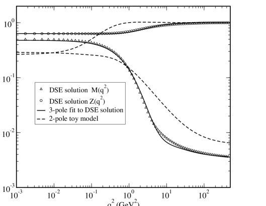
To test the present method, we artificially modify the pole parameterization of the quark propagator so that the lowest pseudo-threshold moves below the vector meson mass, and the latter moves to 0.770 GeV. We achieve this with the following parameterization in terms of $N=2$ pairs of conjugate mass poles

$$m_{1} = -0.400+i0.200~{}{\rm GeV},$$

$$z_{1} = 0.15,$$

$$m_{2} = 0.550+i0.350~{}{\rm GeV},$$

$$z_{2} = 0.35+i0.37~{}~{}.$$ (39)

The resulting propagator amplitudes are also shown in Fig. 2. This parameterization corresponds to $\mu_{1}=$ $0.346~{}{\rm GeV}$, $\Delta_{1}=$ $0.4~{}{\rm GeV}$, and $\mu_{2}=$ $0.424~{}{\rm GeV}$, $\Delta_{2}=$ $0.621~{}{\rm GeV}$. With this propagator, the lowest pseudo-threshold in the BSE is at $2\mu_{1}=$0.692 GeV. The subsequent BSE solution is not to be taken as a physical represenation of the $\rho$ meson; its purpose is to provide a test calculation where the propagator singularities are within the domain of integation.

Figure 3: The eigenvalue $\lambda(P^{2})$ for the vector meson BSE. The mass-shell at $\lambda(-m_{\rho}^{2})=1$, indicated by the vertical line, is above the lowest pseudothreshold set by the complex mass poles of the quark propagators. Proper analytic continuation of the integral produces the solid line; analytic continuation of just the integrand produces the dashed line.

The basis functions used to expand the $q^{2}$ dependence of the BS amplitudes are

$$\phi_{s}(q^{2})=\frac{N_{s}}{\Lambda}L_{s}(w)\;e^{-\frac{w^{2}}{2}}$$ (40)

where $w=q^{2}/\Lambda^{2}$, the typical hadron scale is $\Lambda=$ 0.800 GeV, $L_{s}(w)$ are Laguere polynomials, and $N_{s}$ is fixed by the normalization condition given in Eq. (26). To obtain better than 1% accuracy for the eigenvalue $\lambda(P^{2})$, we found that 7 terms in this basis were sufficient. The number of Chebyshev terms used for the angle basis was one. The first covariant from the set given in Eq. (21) is known to be dominant for the vector meson solution Maris and Tandy (1999) and this was the only one used here.

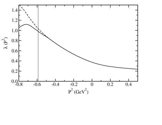
The resulting BSE eigenvalue $\lambda(P^{2})$ is given in Fig. 3 as the solid curve. In the spacelike region ($P^{2}>0$) the eigenvalue is a monotonically, decreasing function of $P^{2}$. When $P^{2}$ decreases below zero and becomes timelike, the eigenvalue $\lambda(P^{2})$ increases for a while then crosses unity, at $P^{2}=-M_{\rho}^{2}$, signifiying a bound state at $M_{\rho}=0.770$ GeV. In Fig. 3 this value of $P^{2}$ is shown as a thin, vertical line. On the timelike side of this line, the eigenvalue continues to increase, then begins to decrease and ultimately goes to zero for ($P^{2}\ll 0$). This is because the eigenvalue is a measure of the magnitude of the BSE kernel and the propagators therein falloff as the difference between the momentum arguments and the pole positions becomes larger than any mass scale in the interaction.

The solid curve in Fig. 3 represents the proper analytic continuation of the BSE from $P^{2}>0$ to $P^{2}<0$. The dashed line represents the result from a direct evaluation of the BSE integral without regard to the possibility of singularities and their movement as a function of $P^{2}$ in relation to the integration domain. That is, only a transcription from $P^{2}>0$ to $P^{2}<0$ has been made in the integrand of Eq. (35); the Feynman technique for combining the denominators and shifting the 4-momentum variable to complete the square has not been made. The integration variables are $q^{2}$ and $z_{q}=\hat{q}\cdot\hat{P}$. It is clear that for the spacelike domain ($P^{2}>0$), and for the limited timelike domain for which no poles move into the domain of integration ($-4\mu_{1}^{2}<P^{2}<0$, i.e., below the lowest pseudo-threshold), the two approaches give identical results. The dashed line represents the approach to the BSE that has usually been implemented; it has been limited to states light enough to avoid the propagator singularities.

With the parameters given above, the quark poles are first encountered within the BSE integration when the analytic continuation reaches $P^{2}=-4\mu_{1}^{2}$, that is, at $P^{2}=-0.48~{}{\rm GeV}^{2}$. Although the contibutions of the conjugate pair of poles to the imaginary part of the BS eigenvalue $\lambda(P^{2})$ cancel, their real contribution produces a discontinuity in the derivative $\lambda^{\prime}(P^{2})$ at that point. Careful inspection of the solid curve in Fig. 3 reveals that this cusp occurs at the precise value where the full calculation and the naïve calculation diverge.

VI Discussion

We have provided a method to obtain meson bound state solutions from the Bethe-Salpeter equation in Euclidean metric when the dressed quark propagators have time-like complex conjugate mass poles within the integration domain. This approximates features encountered in recent QCD modeling via the Dyson-Schwinger equations; the absence of real mass poles simulates quark confinement. For this exploratory study we represent the quark propagators as a sum of complex-conjugate mass poles, and project the BSE on to complete basis sets to represent the momentum and angle dependence. We use Feynman integral techniques to combine the propagator denominators and map the integration to a one-dimensional domain. This allows a clear analysis of the analytic continuation in total meson momentum needed to reach the mass shell and which causes the singularities to impinge upon the integration domain. The BSE linear eigenvalue remains real; in other words the eigenmass remains real. The would-be decay width from one pole is exactly cancelled by the effect of the partner pole; the meson is stable against decay into a quark-antiquark pair. This describes the confinement of quark and antiquark within the meson bound state, even though the meson mass is “above threshold”.

One of the limitations of the method presented here is that it relies upon the projection of the BSE on to a complete basis set of functions to represent the momentum dependence of the BS amplitudes. In general the behavior of the BS amplitudes is not known until after the BSE is solved. If the chosen basis set is an inefficient representation, one would expect this to result in a lack of convergence. The (vector) meson mass that we have studied here is an integrated quantity dominated by infrared physics; it is not surprizing that convergence is easily achieved with the basis states of Eq. (40) which fall off exponentially in the ultraviolet region. However, we know from studies such as Ref. Maris and Tandy (1999) that the leading ultraviolet power law behavior of the vector meson BS amplitudes is $1/q^{2}$. Clearly the present basis would be inefficient for applications that depend strongly on the BS amplitude in this domain, such as the asymptotic behavior of the pion charge form factor Maris and Roberts (1998). For such studies, appropriate basis sets would have to be utilized.

The principal reason that the BS amplitudes are expanded in terms of known basis functions is that the Feynman integral technique for handling the two propagator denominators requires a complex variable shift for the rest of the integrand. In principle, the analytic continuation of the BS amplitude into the complex plane is determined by the dynamics of the BSE and can be determined only through the solution. The implementation of the present method of solution requires a known analytic behavior for the BS amplitudes as expressed through the basis functions. One would expect an inadequacy of the basis in this respect to show up as poor convergence.

Future work using the BSE solution method presented here will include extension of the DSE modeling approach to SU(3) flavor meson states above 1 GeV and meson form factors for $Q^{2}>3~{}{\rm GeV}^{2}$.