Thermal Pions at Finite Isospin Chemical Potential

Abstract

The density corrections, in terms of the isospin chemical potential $\mu_{I}$, to the mass of the pions are studied in the framework of the $SU(2)$ low energy effective chiral lagrangian. The pion decay constant $f_{\pi}(T,\mu_{I})$ is also analized. As a function of temperature for $\mu_{I}=0$, the mass remains quite stable, starting to grow for very high values of $T$, confirming previous results. However, there are interesting corrections to the mass when both effects (temperature and chemical potential) are simultaneously present. At zero temperature the $\pi^{\pm}$ should condensate when $\mu_{I}=\mp m_{\pi}$. This is not longer valid anymore at finite $T$. The mass of the $\pi_{0}$ acquires also a non trivial dependence on $\mu_{I}$ due to the finite temperature.

Pions play a special role in the dynamics of hot hadronic matter since they are the lightest hadrons. Therefore, it is quite important to understand not only the temperature dependence of the pion’s Green functions but also their behavior as function of density, through the chemical potential. The dependence of the pion mass and decay constant on temperature $m_{\pi}(T)$, $f_{\pi}(T)$ has been studied in a variety of frameworks, such as thermal QCD-Sum Rules DFL , Chiral Perturbation Theory (low temperature expansion) GL , the Linear Sigma Model LCL , the Mean Field Approximation Bar1 , the Virial Expansion Schenk , etc. In fact, the pion propagation at finite temperature has been calculated at two loops in the frame of chiral perturbation theory Schenk2 ; T . There seems to be a reasonable agreement that $m_{\pi}(T)$ is essentially independent of $T$, except possibly near the critical temperature $T_{c}$ where $m_{\pi}(T)$ increases with $T$ and that $f_{\pi}(T)$ vanishes for the critical temperature.

The introduction of in-medium processes via isospin chemical potential has been studied at zero temperature son ; toublan ; splittorff in both phases ($|\mu_{I}|\lessgtr m_{\pi}$) at tree level. The problem with both, temperature and density, has been worked out for barionic chemical potential with Chiral Perturbation Theory AE-N . It is also possible to find certain region of the stable pion gas in which the pion number is locally conserved ayala .

Usually, there are two procedures to extract the information of $m_{\pi}$ and $f_{\pi}$ in the frame of chiral perturbation theory. The first one is to compute the Axial-Axial correlator which provides us with the decay constant and the mass corrections. GL ; GL2 ; Schenk2

$$\int d^{4}xe^{ip\cdot x}\langle 0|A_{\mu}^{a}(x)A_{\nu}^{b}(0)|0\rangle=\delta^{ab}\frac{p_{\mu}p_{\nu}f_{\pi}^{2}}{p^{2}-m_{\pi}^{2}}$$ (1)

In the second method, radiative corrections to the propagators are considered together with the realization of PCAC, $\langle 0|A_{\mu}^{a}|\pi^{b}(p)\rangle=ip_{\mu}\delta^{ab}f_{\pi}$ making then use of appropriate counterterms. The use of counterterms is not necessary in the Axial-Axial correlator method. We have checked that both methods leave the same answers. Let us proceed in the frame of the $SU(2)$ chiral perturbation theory. The most general chiral invariant expression for a QCD-extended lagrangian, GL2 ; pich under the presence of external hermitian-matrix auxiliary fields, has the form

$${\cal L}_{\tiny QCD}(s,p,v_{\mu},a_{\mu}) = {\cal L}_{\tiny QCD}^{0}$$ (2)

$$+ \bar{q}\gamma^{\mu}(v_{\mu}+\gamma_{5}a_{\mu})q$$

$$- \bar{q}(s-i\gamma_{5}p)q,$$

where $v_{\mu}$, $a_{\mu}$, $s$ and $p$ are vector, axial, scalar and pseudoscalar fields. The vector current is given by

$$J_{\mu}^{a}=\frac{1}{2}\bar{q}\gamma_{\mu}\tau^{a}q.$$ (3)

When $v,a,p=0$ and $s=M$, being $M=diag(m_{u},m_{d})$ the mass matrix, we obtain the usual $QCD$ lagrangian. This procedure is formal, in the sence that we reproduce the usual QCD lagrangian with current masses. However, we would like to notice that a scalar field in chiral lagrangian models the spontaneus break of chiral symmetry through a non vanishing vacuum expectation value. In this sense if we take for $s=M$, these masses should be actually constituent quark masses, while in the QCD lagrangian we have current masses. Nevertheless this is a formal step which tries only to motivate what follows in the context of effective pion lagrangian.

The effective action with finite isospin chemical potential is given by

$${\cal L}_{\tiny QCD}^{I} = {\cal L}_{\tiny QCD}(M,0,0,0)+\mu^{a}u^{\mu}J^{a}_{\mu}$$ (4)

$$= {\cal L}_{\tiny QCD}(M,0,\mu u_{\mu},0)$$

where $\mu^{a}=(0,0,\mu_{I})$ is the third isospin component, $\mu=\mu^{a}\tau^{a}/2$ and $u_{\mu}$ is the 4-velocity between the observer and the thermal heat bath. This is required in order to describe in a covariant way this system, where the Lorentz invariance is broken since the thermal heath bath represents a privileged frame of reference.

Proceeding in the same way, now in the low-energy description where only pion degrees of freedom are relevant, let us consider the most general chiral invariant lagrangian ordered in a series of powers of the external momentum. We will start with the ${\cal O}(p^{2})$ chiral lagrangian

$${\cal L}_{2} = \frac{f^{2}}{4}Tr\left[(D_{\mu}U)^{\dagger}D^{\mu}U+U^{\dagger}\chi+\chi^{\dagger}U\right]$$ (5)

with

$$D_{\mu}U = \partial_{\mu}U-i[v_{\mu},U]-i\{a_{\mu},U\}$$

$$\chi = 2B(s+ip)$$

$$U = \bar{U}^{\frac{1}{2}}(e^{i\pi^{a}\tau^{a}/f})\bar{U}^{\frac{1}{2}}$$ (6)

$\bar{U}$ is the vacuum expectation value of the field $U$ and $B$ in the previous equation is an arbitrary constant which will be fixed when the mass is identified setting $(m_{u}+m_{d})B=m^{2}$. The most general ${\cal O}(p^{4})$ chiral lagrangian has the form

$${\cal L}_{4} = \alpha_{1}\left(Tr\left[(D_{\mu}U)^{\dagger}D^{\mu}U\right]\right)^{2}$$ (7)

$$+ \alpha_{2}Tr\left[(D_{\mu}U)^{\dagger}D_{\nu}U\right]Tr\left[(D^{\mu}U)^{\dagger}D^{\nu}U\right]$$

$$+ \alpha_{3}\left(Tr\left[\chi U^{\dagger}+U\chi^{\dagger}\right]\right)^{2}$$

$$+ \alpha_{4}Tr\left[(D_{\mu}U)^{\dagger}D^{\mu}U\right]Tr\left[\chi U^{\dagger}+U\chi^{\dagger}\right]$$

$$+ \alpha_{5}\left[L_{\mu\nu}UR^{\mu\nu}U^{\dagger}\right]$$

$$+ i\alpha_{6}Tr\left[L_{\mu\nu}D^{\mu}U(D^{\nu}U)^{\dagger}+R_{\mu\nu}(D^{\mu}U)^{\dagger}D^{\nu}U\right]$$

$$+ \alpha_{7}\left(Tr\left[\chi U^{\dagger}-U\chi^{\dagger}\right]\right)^{2}$$

$$+ \alpha_{8}Tr\left[\chi U^{\dagger}\chi U^{\dagger}+U\chi^{\dagger}U\chi^{\dagger}\right]$$

$$+ \alpha_{9}Tr\left[L_{\mu\nu}L^{\mu\nu}+R_{\mu\nu}R^{\mu\nu}\right]$$

$$+ \alpha_{10}Tr[\chi^{\dagger}\chi]$$

with

$$L_{\mu\nu}=\partial_{\mu}l_{\nu}-\partial_{\nu}l_{\mu}+i[l_{\mu},l_{\nu}], \quad l_{\mu}=v_{\mu}-a_{\mu}$$

$$R_{\mu\nu}=\partial_{\mu}r_{\nu}-\partial_{\nu}r_{\mu}+i[r_{\mu},r_{\nu}], \quad r_{\mu}=v_{\mu}+a_{\mu}$$ (8)

The different coupling constants $\alpha_{i}$in the previous expression are related to the couplings introduced by GL1 . Here we use the prescription of Scherer .

The effective action with finite chemical potential in terms of pion degrees of freedom has the same form as eq.4, where the different external fields are defined in eq.6. In this paper we will consider one loop corrections, up to the fourth order in the fields, to the lagrangian ${\cal L}_{2}$ and the free part, i.e the tree level part of ${\cal L}_{4}$ with renormalized fields. This procedure is standard, GL2 ; holstein . We will concentrate on the phase where $\mu_{I}<m_{\pi}$, where the vacuum expectation value $\bar{U}=1$. The interacting part ${\cal L}_{4}$ involves higher powers in the momentum of the pion fields. The constants $\alpha_{i}$ present in ${\cal L}_{4}$ are known from decay and scattering measurements. Therefore, we have the following lagrangians ${\cal L}_{i,j}$

$${\cal L}_{2,2} = \frac{1}{2}\left[\left(\partial\pi_{0}\right)^{2}-m^{2}\pi_{0}^{2}\right]+\left|\partial_{I}\pi\right|^{2}-m^{2}\left|\pi\right|^{2}$$

$${\cal L}_{2,4} = \frac{1}{4!}\frac{m^{2}}{f^{2}}\pi_{0}^{4}+\frac{1}{6f^{2}}\left[-4\left|\partial_{I}\pi\right|^{2}\left|\pi\right|^{2}\right.$$

$$\qquad\qquad\qquad\left.+\left(\partial\left|\pi\right|^{2}\right)^{2}+m^{2}\left(\left|\pi\right|^{2}\right)^{2}\right]$$

$$+\frac{1}{6f^{2}}\left[-2\left|\partial_{I}\pi\right|^{2}\pi_{0}^{2}-2\left(\partial\pi_{0}\right)^{2}\left|\pi\right|^{2}\right.$$

$$\qquad\quad\left.+\partial\pi_{0}^{2}\cdot\partial\left|\pi\right|^{2}+m^{2}\pi_{0}^{2}\left|\pi\right|^{2}\right]$$

$${\cal L}_{4,2} = 2\frac{m^{2}}{f^{2}}\left[l_{4}\left|\partial_{I}\pi\right|^{2}-m^{2}(l_{3}+l_{4})\left|\pi\right|^{2}\right.$$ (9)

$$+\left.\frac{1}{2}l_{4}\left(\partial\pi_{0}\right)^{2}-\frac{1}{2}m^{2}(l_{3}+l_{4}-\epsilon_{ud}^{2}l_{7})\pi_{0}^{2}\right]$$

with $l_{i}$ the original parameters of Gasser & Leutwyler $SU(2)$ lagrangian

$$l_{4} = 8\alpha_{4}$$

$$l_{3} = 16\alpha_{3}+8\alpha_{8}-8\alpha_{4}$$

$$l_{7} = -16\alpha_{7}-8\alpha_{8}$$ (10)

where the subindexes ($i,j$) in the lagrangian denote the order in powers of momentum and fields, respectively, and

$$\partial_{I\pm}\equiv\partial\pm i\mu_{I}u.$$

This definition of the covariant derivative is natural, since we know weldon ; actor that the chemical potential is introduced as the zero component of an external “gauge” field. In the previous expression,

$$|\pi|^{2}\equiv\pi^{+}\pi^{-},\qquad|\partial_{I}\pi|^{2}=(\partial_{I}\pi)_{+}(\partial_{I}\pi)_{-}.$$

We will neglect $\epsilon_{ud}^{2}=(m_{u}-m_{d})^{2}/(m_{u}+m_{d})^{2}$ because it only shifts in a small quantity the neutral pion mass and we are interested in the thermal and density evolution of the masses.

For renormalizing with counterterms we introduce the following decomposition

$${\cal L}_{eff} = {\cal L}_{2,2}+{\cal L}_{2,4}^{r}+{\cal L}^{r}_{4,2}$$

$${\cal L}_{2,2} = {\cal L}^{r}_{2,2}+\delta{\cal L,}$$ (11)

where the $r$ index denote the lagrangian with renormalized fields.

Setting $\pi_{0}=\sqrt{Z_{0}}\pi_{0}^{r}$ and $\pi_{\pm}=\sqrt{Z_{\pm}}\pi_{\pm}^{r}$ in ${\cal L}_{2,2}$, we have

$$\delta{\cal L} = \frac{1}{2}\delta_{Z_{o}}\left[(\partial\pi_{0}^{r})^{2}-m^{2}(\pi_{0}^{r})^{2}\right]$$ (12)

$$+\delta_{Z_{\pm}}\left[\left|\partial_{I}\pi^{r}\right|^{2}-m^{2}\left|\pi^{r}\right|^{2}\right]$$

with $\delta_{Z_{i}}=Z_{i}-1$.

First, let us consider the temperature and density corrections to the pion propagator. Since our calculation will be at the one loop level, we do not need the full formalism of thermo field dynamics, including thermal ghosts and matrix propagators. The propagator

$$D_{\pm}(x)=D(x;\pm\mu_{I})+D_{\beta}(x;\pm\mu_{I})$$ (13)

for charged pions at the tree level will be given by an extension, for a non-vanishing chemical potential, of the well known Dolan-Jackiw propagators for scalar fields weldon . Note that since there is no chemical potential associated to the neutral pion, the thermal propagator $D_{0}$ will be the usual one

$$D_{0}(x)=D(x;0)+D_{\beta}(x;0)$$ (14)

where, in momentum space

$$\underline{\mathrm{D}}(k;\pm\mu_{I}) = \frac{i}{k_{\pm}^{2}-m^{2}+i\epsilon}$$

$$\underline{\mathrm{D}}_{\beta}(k;\pm\mu_{I}) = 2\pi n_{B}(|k\cdot u|)\delta(k_{\pm}^{2}-m^{2})$$ (15)

with

$$k_{\pm}\equiv k\mp\mu_{I}u,\qquad n_{B}(x)=\frac{1}{e^{\beta x}-1}$$

are the shifted momentum and the Bose-Einstein factor.

We will use the $\overline{MS}$-scheme, and we renormalize as usual at $T=0$, since the thermal corrections are finite. The self energy for charged and neutral pions including the counterterms has the form

$$\Sigma_{\pm}(p) = [A_{\pm}-\delta_{Z_{\pm}}]p_{\pm}^{2}-[A_{\pm}^{\prime}-\delta_{Z_{\pm}}]m^{2}+A_{\pm}^{\prime\prime}u\cdot p_{\pm}$$

$$\Sigma_{0}(p) = [A_{0}-\delta_{Z_{0}}]p^{2}-[A_{0}^{\prime}-\delta_{Z_{0}}]m^{2}$$ (16)

with

$$A_{\pm} = \frac{1}{3f^{2}}\left[D_{\pm}(0)+D_{0}(0)\right]-2\frac{m^{2}}{f^{2}}l_{4}$$

$$A_{\pm}^{\prime} = \frac{1}{6f^{2}}\left[2D_{\pm}(0)-D_{0}(0)\right]-2\frac{m^{2}}{f^{2}}(l_{3}+l_{4})$$

$$A_{\pm}^{\prime\prime} = \frac{2}{f^{2}}u\cdot\partial D_{\pm}(0)$$

$$A_{0} = \frac{2}{3f^{2}}D_{\pm}(0)-\frac{m^{2}}{f^{2}}l_{4}$$

$$A_{0}^{\prime} = \frac{1}{6f^{2}}\left[3D_{0}(0)-2D_{\pm}(0)\right]-\frac{m^{2}}{f^{2}}(l_{3}+l_{4})$$ (17)

Our prescription to fix the counterterm $\delta_{Z_{\pm}}$ is to impose that $\Sigma$ does not depend on $p^{2}$, so, $\delta_{Z_{i}}=A_{i}$. In this way, the renormalized propagators will take the form

$$i\underline{\mathrm{D}}_{\pm}^{r}(p)^{-1} = p_{\pm}^{2}-A_{\pm}^{\prime\prime}u\cdot p_{\pm}-m^{2}[1-A_{\pm}^{\prime}+A_{\pm}]$$

$$i\underline{\mathrm{D}}_{0}^{r}(p)^{-1} = p^{2}-m^{2}[1-A_{0}^{\prime}+A_{0}]$$ (18)

where $\alpha_{i}$ terms absorbs the divergences

$$\l_{i} = \frac{\gamma_{i}}{32\pi^{2}}\left[\bar{\l}_{i}+\ln\frac{4\pi m^{2}}{\Lambda^{2}}-\frac{2}{d-4}-\gamma+1\right]$$ (19)

in which the $\gamma_{i}$ terms are tabulated GL2 ; holstein , being $\Lambda$ a scale factor.

We identify $m_{\pi^{+}}$ and $m_{\pi^{-}}$ from the solution of $\underline{\mathrm{D}}_{\pm}^{r}(p)^{-1}|_{{\bf p}=0}=0$ in the frame where the heath bath is at rest ($u=(1,{\bf 0})$). We get the well known result for $T=\mu_{I}=0$

$$m_{\pi}=m\left(1-\alpha_{\pi}\bar{l}_{3}/4\right)$$ (20)

is identified with the physical mass. $\alpha_{\pi}=(m_{\pi}/4\pi f_{\pi})^{2}$ is the perturbative term that fixes the scale of energies in the theory (for energies below $4\pi f_{\pi}$) so we neglect the ${\cal O}(g^{2})$ factors. This allows us to set $m\approx m_{\pi}$ in all radiative corrections (and also $f\approx f_{\pi}$). The procedure is the same for $m_{\pi^{0}}$

It is important to remark that radiative corrections will leave a dependence on the chemical potential for the pion mass only for finite values of temperature. In a strict sense, this procedure does not allow us to say nothing new for an eventual chemical potential dependence of the masses at $T=0$ (cold matter) which is already included in ${\cal L}_{2}$. In this case, $T=0$, we have to follow the usual procedure, son ; toublan , of computing the minimum of the effective potential in ${\cal L}_{2}$ when the chemical potential is taken into account, without considering radiative corrections. This enables to identify a phase structure where a non trivial vacuum appears for higher values of $\mu_{I}$, $|\mu_{I}|>m_{\pi}$characterized by the appearance of a condensate $\langle\pi^{-}\rangle$. (The opposite occurs for negative values of the chemical potential, where the vacuum state is a condensate $\langle\pi^{+}\rangle$). At $T=0$ when $\mu_{I}=m_{\pi}$, the mass of $\pi^{-}$ vanishes.

For finite $T$ and $\mu_{I}$, we find the following expression for the masses

$$m_{\pi^{\pm}}(T,\mu_{I})\!\! = \!\!m_{\pi}\left[1+\alpha_{\pi}I_{0}\pm\left(\mu_{I}/m_{\pi}-4\alpha_{\pi}J\right)\right]$$

$$m_{\pi^{0}}(T,\mu_{I})\!\! = \!\!m_{\pi}\left[1+\alpha_{\pi}\left(2I-I_{0}\right)\right]$$ (21)

with

$$I = \int_{1}^{\infty}dx\sqrt{x^{2}-1}[n_{B}(m_{\pi}x-\mu_{I})+n_{B}(m_{\pi}x+\mu_{I})]$$

$$J = \int_{1}^{\infty}dxx\sqrt{x^{2}-1}[n_{B}(m_{\pi}x-\mu_{I})-n_{B}(m_{\pi}x+\mu_{I})]$$

$$I_{0} = I(\mu_{I}=0)$$ (22)

Note that our convention for the chemical potential sign is contrary to the one adopted in the paper by Kogut and Toublan toublan , who extended previous results by Son and Stephanov son .

If the chemical potential of the charged pions vanishes, i.e for symmetric matter, at finite T we get the well known result for $m_{\pi}(T)$ due to chiral perturbation theory GL , see also LCL . However, due to radiative corrections to the neutral pion propagator, its mass will acquire a non trivial chemical potential dependence for finite values of temperature. In the approach where the minimum of the effective potential is calculated (for finite $\mu_{I}$ and $T=0$), the mass of the neutral pion remains constant.

We show in Fig.1 a tridimensional picture for the behavior of the mass of the neutral pion. Note that when $\mu_{I}=0$, $m_{\pi_{0}}(T)=m_{\pi^{\pm}}(T)$.

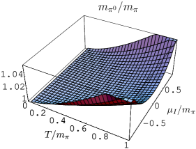
Figure 1: $m_{\pi^{0}}$ as function of $T$ and $\mu_{I}$ in units of $m_{\pi}$

From Fig.2 we see that at zero temperature, we agree with the usual prediction, $m_{\pi}^{+}=m_{\pi}+\mu_{I}$. In fact, at zero temperature the $\pi^{+}$ should condensate when $\mu_{I}=-m_{\pi}$ (the inverse situation occurs for $\pi^{-}$). Now, this situation changes if temperature starts to grow. The condensation point disappear at $\mu_{I}=-m_{\pi}$; in $\mu_{I}=m_{\pi}$ the mass start to decrease. For small $T$ (for example inside an neutron star), this effect is neglegible.

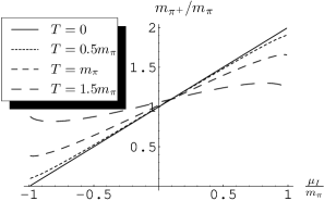
Figure 2: $m_{\pi^{+}}$ as function of $\mu_{I}$ for a fixed $T$

In connection with the behavior of $f_{\pi}(T,\mu_{I})$ when $\mu_{I}<m_{\pi}$, we have make used of PCAC, which provides us with a relation between the renormalized propagator and the pion decay constant.

The Axial current is obtained as the functional derivative of the action with respect to $a_{\mu}^{a}$, with $a_{\mu}=a_{\mu}^{a}\tau^{a}/2$

$$A_{\mu}^{a}=\frac{\delta{\cal S}}{\delta a_{\mu}^{a}}(M,0,\mu u_{\mu},0)$$ (23)

The axial current is

$$A_{(1,1)\mu}^{\pm} = -f(\partial_{\mu}^{I}\pi)^{\pm}$$

$$A_{(1,3)\mu}^{\pm} = \frac{2}{3f}\left\{\pi^{0}\left[\pi^{0}(\partial_{\mu}^{I}\pi)^{\pm}-\pi^{\pm}\partial_{\mu}\pi^{0}\right]\right.$$

$$\left.+\pi^{\pm}\left[\pi^{\mp}(\partial_{\mu}^{I}\pi)^{\pm}-\pi^{\pm}(\partial_{\mu}^{I}\pi)^{\mp}\right]\right\}$$

$$A_{(3,1)\mu}^{\pm} = -\frac{m^{2}}{f}2l_{4}(\partial_{\mu}^{I}\pi)^{\pm}$$

$$A_{(1,1)\mu}^{0} = -f\partial_{\mu}\pi^{0}$$

$$A_{(1,3)\mu}^{0} = \frac{2}{3f}\left\{2|\pi|^{2}\partial_{\mu}\pi^{0}-\pi^{0}\partial_{\mu}|\pi|^{2}\right\}$$

$$A_{(3,1)\mu}^{0} = -\frac{m^{2}}{f}2l_{4}\partial_{\mu}\pi^{0}$$ (24)

Now, the effective axial current at ${\cal O}(p^{3})$ will be

$$A_{\mu}^{i} \equiv A_{(1,1)\mu}^{i}+A_{(1,3)\mu}^{ir}+A_{(3,1)\mu}^{ir}$$ (25)

$$= \sqrt{Z_{i}}A_{(1,1)\mu}^{ir}+A_{(1,3)\mu}^{ir}+A_{(3,1)\mu}^{ir}$$

with $i=\{\pm,0\}$. We will take

$$\sqrt{Z_{i}}=\sqrt{1+\delta_{Z_{i}}}\simeq 1+\frac{1}{2}\delta_{Z_{i}}+{\cal O}(\delta_{Z_{i}}^{2}).$$

The value of the $\delta_{Z_{i}}$ are the same as those obtained in the mass renormalization.

After taking into account the different tadpole diagrams which correct the coupling of the current to one pion states, we find

$$\langle 0|A_{\mu}^{\pm}|\pi^{\mp}(p)\rangle = ip_{\pm\mu}\left[f_{\pi}-f2\alpha_{\pi}(I+I_{0})\right]$$

$$\pm iu_{\mu}f\alpha_{\pi}8J$$

$$\langle 0|A_{\mu}^{0}|\pi^{0}(p)\rangle = ip_{\mu}\left[f_{\pi}-f4\alpha_{\pi}I\right]$$ (26)

with

$$f_{\pi} = f\left(1+\alpha_{\pi}\bar{l}_{4}\right)$$ (27)

Now, we can set $f\simeq f_{\pi}$, $m\simeq m_{\pi}$ in all ${\cal O}(\alpha_{\pi})$ terms, since any correction will be of order $\alpha_{\pi}^{2}$ (including $\alpha_{\pi}$), then we define the effective decay constant as the part proportional to $p_{\mu}$, so

$$f_{\pi^{\pm}}(T,\mu_{I}) \equiv f_{\pi}[1-2\alpha_{\pi}(I+I_{0})]$$

$$f_{\pi^{0}}(T,\mu_{I}) \equiv f_{\pi}[1-4\alpha_{\pi}I]$$ (28)

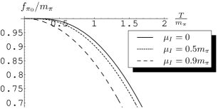
Figure 3: $f_{\pi_{0}}$ as function of $T$ for a fixed $\mu_{I}$

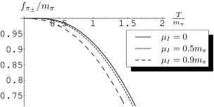
Figure 4: $f_{\pi^{\pm}}$ as function of $T$ for a fixed $\mu_{I}$

For $\mu_{I}=0$ we agree with the well known results of Gasser and Leutwyler GL . For an increasing finite chemical potential, the $f_{\pi}(T)$ couplings decrease faster. This effect is enhanced for $f_{\pi_{0}}(T)$ and is related to the fact that $f_{\pi_{0}}(T)$only receives radiative corrections from charged pion tadpoles.

In heavy ion collisions, a finite value of $\mu_{I}$ means that, at least locally, we would expect more pions with definite charge than in the symmetric case. According to this picture, the production rate of dileptons from pion annhilation should be supressed. Probably, the detection of such kind of effects will demand a higher center of mass energy.

Figure 5: $T$,$\mu_{I}$ phase diagram for pion condensation

In order to explore the region where $|\mu_{I}|>m_{\pi}$, associated to a new phase where the condensates occur, we need to redefine our fields as fluctuations around the configuration corresponding to a minima of the effective potential in ${\cal L}_{2}$. At present we are working on it, but it is possible to extrapolate, for $T\ll m_{\pi}$ and $\mu_{I}\sim m_{\pi}$ the condensation point in such a way that we actually remain in the first phase. However the curve in the $\mu_{I}-T$ plane that separates both phases is only reliable in the parameters region mentioned before where in the thermal factors in eq.(22), we have taken the approximation $n_{B}(m_{\pi}x\pm\mu_{I})\simeq exp[-\beta(m_{\pi}x\pm\mu_{I})]$. A complete analysis of the phase can be found in splittorff2 . The phase diagram is shown in Fig. 5 in accordance with son . However, for higher values of $\mu_{I}$ changes abruptly and our approximation is no longer valid.

Acknowledgements: The work of M.L. has been supported by Fondecyt (Chile) under grant No.1010976. C.V. acknowledges support from a Conicyt Ph.D fellowship (Beca Apoyo Tesis Doctoral).

References

(1) C. A. Dominguez, M. S. Fetea and M. Loewe, Phys. Lett. B 387
151 (1996) ; C. A. Dominguez, M. loewe, and J. C. Rojas, Phys. Lett. B 320 377 (1994)
(2) J. Gasser and H. Leutwyler, Phys. Lett. B 184 83 (1987) .
(3) A. Larsen, Z. Phys. C 33 291
(1986) ; C. Contreras and M. Loewe, Int. J. Mod. Phys. A 5
2297 (1990) .
(4) A. Barducci, R. Casalbuoni, S. DeCurtis, R. Gatto, and G.
Pettini, Physical Review D 46, 2203 (1992) .
(5) A. Schenk, Nucl. Phys. B 363 97 (1991) .
(6) A. Schenk, Phys. Rev. D 47, 5138 (1993).
(7) D. Toublan, Phys. Rev. D 56, 5629 (1997).
(8) D. T. Son and M. A. Stephanov, Phys. Rev. Lett. 86 592 (2001) ; QCD at
finite isospin density: from pion to quark-antiquark condensation,
published in Phys. Atom. Nucl. 64 834 (2001) , Yad. Fiz 64 899 (2001).
(9) J. B. Kogut and D. Toublan, Physical Review D 64, 034007 (2001).
(10) K. Splittorff, D Toublan, J.J.M.
Verbaarschot, Nucl. Phys B 620 290 (2002)
(11) J. Gasser and H. Leutwyler, Ann. Phys. 158 142 (1984).
(12) R. Alvarez-Estrada and A. Gómez Nicola, Phys
Lett. B 355 288 (1995)
(13) A. Ayala, P. Amore, A. Aranda, Phys. Rev. C 66, 045205 (2002).
A. Ayala, hep-ph/0212320
(14) S. Scherer, hep-ph/0210398
(15) R. D. Pisarski, Phys. Lett. B 110 155 (1982).
(16) H. Leutwyler and A. V. Smilga, Nucl. Phys. B 342
(1990) 302.
(17) C. A. Dominguez, M. Loewe, and J. C. Rojas,
Z. Phys. C 59 63 (1993).
(18) J. Gasser and H. Leutwyler, Nucl. Phys. B 250
465 (1985).
(19) A. Pich, Introduction to Chiral Perturbation Theory, CERN-TH. 6978/93,
Lectures given at the V Mexican School of Particles and Fields.
(20) J. F. Donoghue, E. Golowich, and B. R. Holstein, Dynamics of the Standard Model (Cambridge University Press, 1992).
(21) H. A. Weldon, Phys. Rev. D 26 1394
(1982), Nucl. Phys. B 270 79 (1986).
(22) A. Actor, Phys. Rev. D 27 2548 (1983), Phys. Lett. B 175 53
(1985).
(23)K. Splittorff, D Toublan, J.J.M.
Verbaarschot, Nucl.Phys. B 639 524(2002)