$B\rightarrow KK$ decays with the soft-gluon corrections

Abstract

We analyze the $B\rightarrow KK$ decays with the soft-gluon corrections by using the QCD light-cone sum rules (LCSR). Although QCD factorization approach calculates the leading order factorization parts and the radiative corrections from hard- gluon exchanges at $\alpha_{s}$ order, it is worthwhile to estimate the nonfactorizable soft-gluon contributions from all the tree and penguin diagrams systematically. Our results show that the soft-gluon effects always decrease the branching ratios and give a few percentage corrections at most in the $B\rightarrow KK$ decays.

Key Words: B meson decays, QCD light-cone sum rules, QCD factorization approach

I INTRODUCTION

Recently, A. Khodjamirian s1 has presented an approach to calculate the hadronic matrix elements of nonleptonic B meson decays within the framework of the light-cone sum rules, where the nonfactorizable soft contributions can be effectively dealt with. As we know, QCD factorization approach s2 provided that the hadronic matrix elements for $B\rightarrow\pi\pi,K\pi$ decays can be expanded in the powers of $\alpha_{s}$ and $\frac{\Lambda_{QCD}}{m_{b}}$ and exhibited a considerablly strong predicative potential. However, this approach can’t calculate $\frac{\Lambda_{QCD}}{m_{b}}$ corrections quantitatively, such as the nonfactorizable contributions from the soft-gluon exchanges. Thus it is interesting to evaluate the corrections from the soft-gluon exchanges by using light-cone QCD sum rules.

In the previous paper s3 , the role of the soft-gluon exchanges in $B\rightarrow\pi\pi$ has been studied by using the light-cone QCD sum rules. Compared to the Ref. s1 , the calculations are carried out not only for the tree operators but also for the penguin ones. Ref.s3 showed that the $\frac{\Lambda_{QCD}}{m_{b}}$ corrections from the soft-gluon exchanges are not always negligible in the process $B\rightarrow\pi\pi$ and the nonfactorizable soft contributions are almost as important as the $O(\alpha_{s})$ correction parts, and in some cases even have the same order effects as that of the factorization amplitude. Therefore it is worthwhile to evaluate the nonfactorizable soft-gluon contributions in the process $B\rightarrow KK$.

II CORRELATOR AND SUM RULES

Similar to the case of $B\rightarrow\pi\pi$, we can calculate the contributions from the soft-gluon exchanges in $B\rightarrow KK$ including the tree and penguin operators. We begin with the effective Hamiltonian $H_{eff}$ which is responsible for the $B\rightarrow KK$ decays s4 :

$${\cal H}_{eff}= \frac{G_{F}}{\sqrt{2}}[V_{ub}V_{uq}^{*}(c_{1}(\mu)O_{1}(\mu)+c_{2}(\mu)O_{2}(\mu))$$ (1)

$$-V_{tb}V_{tq}^{*}\sum\limits_{i=3}^{10}c_{i}O_{i}]+h_{.}c_{.}$$

where $O_{1,2}$ are the tree operators and $O_{3}-O_{10}$ denote the penguin ones. By applying the Fierz transformation, the operators which is related to the soft corrections to $B\rightarrow KK$ can be clearly presented in effective weak Hamiltonian:

$${\cal H}_{eff}=\frac{G_{F}}{\sqrt{2}}[V_{ub}V_{ud}^{*}(c_{1}(\mu)+\frac{c_{2}(\mu)}{3})O_{1}(\mu)+2c_{2}(\mu)\widetilde{O}_{1}(\mu)+\cdots],$$ (2)

where

$${O}_{1}=(\overline{s}\Gamma_{\mu}u)(\overline{u}\Gamma^{\mu}b),$$ (3)

and

$$\widetilde{O}_{1}=(\overline{s}\Gamma_{\mu}\frac{\lambda^{a}}{2}u)(\overline{u}\Gamma^{\mu}\frac{\lambda^{a}}{2}b),$$ (4)

the penguin operators are denoted by ellipses. In the above $\Gamma_{\mu}=\gamma_{\mu}(1-\gamma_{5})$, $Tr(\lambda^{a}\lambda^{b})=2\delta^{ab}$. To the operator $O_{1}$, we employ the results of QCD factorization approach directly to the contributions from the factorizaton and $\alpha_{s}$ corrections since the result of LCSR is consistent with the prediction of the QCD factorization approach.

In order to calculate the nonfactorizable matrix elements induced by the operator $\widetilde{O}_{1}$, we choose a proper vaccum-kaon correlation function:

$$F_{\alpha}^{(\widetilde{O}_{1})}(p,q,k)=-\int d^{4}xe^{-i(p-q)x}\int d^{4}ye^{i(p-k)}\langle 0|T\{j_{\alpha 5}^{(K)}(y)\widetilde{O}_{1}(0)j_{5}^{(B)}(x)\}|K^{-}(q)\rangle,$$ (5)

where $j_{\alpha 5}^{(K)}=\overline{u}\gamma_{\alpha}\gamma_{5}s$ and $j_{5}^{(B)}=m_{b}\overline{b}i\gamma_{5}d$ are the quark currents interpolating $K$ and $B$ mesons, respectively. The decomposition of the correlation function Eq.(5) in terms of independent momenta is straightforward and contains four invariant amplitudes:

$$F_{\alpha}^{(\widetilde{O}_{1})}=(p-k)_{\alpha}F^{(\widetilde{O}_{1})}+q_{\alpha}\tilde{F_{1}}^{(\widetilde{O}_{1})}+k_{\alpha}\tilde{F_{2}}^{(\widetilde{O}_{1})}+\epsilon_{\alpha\beta\lambda\rho}q^{\beta}p^{\lambda}k^{\rho}\tilde{F_{3}}^{(\widetilde{O}_{1})}.$$ (6)

In what follows only the amplitude $F^{(\widetilde{O}_{1})}$ is relevant. To obtain $F^{(\widetilde{O}_{1})}$, we calculate the correlation function by expanding the T-product of three operators, two currents and $\widetilde{O}_{1}$, near the light-cone $x^{2}\sim y^{2}\sim(x-y)^{2}\sim 0$. To stay away from hadronic thresholds in both channels of $K$ and $B$ currents, we choose the following kinematical region in Eq.(5):

$$q^{2}=p^{2}=k^{2}=0\quad\mbox{and}\quad|(p-k)^{2}|\sim|(p-q)^{2}|\sim|P^{2}|\gg{\Lambda_{QCD}}^{2},$$ (7)

where $P\equiv p-k-q$.

Following the standard procedure for QCD sum rule calculation, we can obtain:

$$A^{(\widetilde{O}_{1})}(B\rightarrow KK)= \langle K(p),K(-q)|\widetilde{O}_{1}|B(p-q)\rangle$$ (8)

$$=\frac{-i}{\pi^{2}f_{K}f_{B}{m_{B}}^{2}}\int_{0}^{s_{0}^{K}}dse^{\frac{-s}{M^{2}}}\int_{m_{b}^{2}}^{\bar{R}(s,m_{b}^{2},m_{B}^{2},s_{0}^{B})}ds^{\prime}$$

$$e^{\frac{m_{B}^{2}-s^{\prime}}{{M^{\prime}}^{2}}}Im_{s^{\prime}}Im_{s}F_{QCD}^{(\widetilde{O}_{1})}(s,s^{\prime},m_{B}^{2}),$$

where $s_{0}^{K}$ and $s_{0}^{B}$ are effective threshold parameters. A straightforward calculation gives the following results for the twist-3 and twist-4 contributions:

$$F^{(\widetilde{O}_{1})}_{QCD}=F_{tw3}^{(\widetilde{O}_{1})}+F_{tw4}^{(\widetilde{O}_{1})},$$ (9)

with

$$F_{tw3}^{(\widetilde{O}_{1})}= \frac{m_{b}f_{3{K}}}{4{\pi}^{2}}\int_{0}^{1}dv\int D\alpha_{i}$$ (10)

$$\times\frac{\varphi_{3K}(\alpha_{i})}{(m_{b}^{2}-(p-q)^{2}(1-\alpha_{1}))(-P^{2}v\alpha_{3}-(p-k)^{2}(1-v\alpha_{3}))}$$

$$\times[(2-v)(q\cdot k)+2(1-v)q\cdot(p-k)](q\cdot(p-k)),$$

and

$$F_{tw4}^{(\widetilde{O}_{1})}= -\frac{m_{b}^{2}f_{K}}{4{\pi}^{2}}\int_{0}^{1}dv\int D\alpha_{i}\widetilde{\varphi}_{\perp}(\alpha_{i})\frac{1}{m_{b}^{2}-(p-q+q\alpha_{1})^{2}}\frac{(4v-6)(p-k)q}{(p-k-qv\alpha_{3})^{2}}$$ (11)

$$+\frac{m_{b}^{2}f_{K}}{2{\pi}^{2}}\int_{0}^{1}dv\int d\alpha_{1}d\alpha_{3}\Phi_{1}(\alpha_{1},\alpha_{3})\frac{1}{[m_{b}^{2}-(p-q+q\alpha_{1})^{2}]^{2}}\frac{(2pq-2vqk)(p-k)q}{(p-k-qv\alpha_{3})^{2}}$$

$$-\frac{m_{b}^{2}f_{K}}{2{\pi}^{2}}\int_{0}^{1}dv\int d\alpha_{3}\Phi_{2}(\alpha_{3})\frac{1}{[m_{b}^{2}-(p-q\alpha_{3})^{2}]^{2}}\frac{(2pq-2vqk)(p-k)q}{(p-k-qv\alpha_{3})^{2}}$$

$$+\frac{m_{b}^{2}f_{K}}{2{\pi}^{2}}\int_{0}^{1}dv2v^{2}\int d\alpha_{3}\Phi_{2}(\alpha_{3})\frac{1}{pq[m_{b}^{2}-(p-q\alpha_{3})^{2}]}\frac{[(p-k)q]^{3}}{(p-k-qv\alpha_{3})^{4}}$$

$$-\frac{m_{b}^{2}f_{K}}{2{\pi}^{2}}\int_{0}^{1}dv(2v-2)v\int d\alpha_{3}\Phi_{2}(\alpha_{3})\frac{1}{m_{b}^{2}-(p-q\alpha_{3})^{2}}\frac{[(p-k)q]^{2}}{(p-k-qv\alpha_{3})^{4}},$$

where the definitions of $\varphi_{3K}(\alpha_{i})$, $\varphi_{\parallel}(\alpha_{i})$ and $\varphi_{\perp}(\alpha_{i})$ can be found in Ref.s5 .

By taking the duality approximation and applying Borel transformation, we get the following sum rule:

$$A^{(\widetilde{O}_{1})} (B\rightarrow KK)$$ (12)

$$=im_{B}^{2}(\frac{1}{4{\pi}^{2}f_{K}}\int_{0}^{s_{0}^{K}}dse^{-\frac{s}{M^{2}}})(\frac{m_{b}^{2}}{2f_{B}m_{B}^{4}}\int_{u_{0}^{B}}^{1}\frac{du}{u}e^{\frac{m_{B}^{2}}{{M^{\prime}}^{2}}-\frac{m_{b}^{2}}{u{M^{\prime}}^{2}}}$$

$$\times[\frac{m_{b}f_{3K}}{u}\int_{0}^{u}\frac{dv}{v}\varphi_{3K}(1-u,u-v,v)+f_{K}\int_{0}^{u}\frac{dv}{v}[3\widetilde{\varphi}_{\perp}(1-u,u-v,v)$$

$$-(\frac{m_{b}^{2}}{u{M^{\prime}}^{2}}-1)\frac{\Phi_{1}(1-u,v)}{u}]+f_{K}(\frac{m_{b}^{2}}{u{M^{\prime}}^{2}}-2)\frac{\Phi_{2}(u)}{u^{2}}]),$$

where the light-cone wave functions are introduced as the following:

$$\frac{\partial{\Phi_{1}}(w,v)}{\partial v}=\widetilde{\varphi}_{\perp}(w,1-w-v,v)+\widetilde{\varphi}_{\parallel}(w,1-w-v,v)$$

$$\frac{\partial{\Phi_{2}}(v)}{\partial v}=\Phi_{1}(1-v,v),$$ (13)

For the kaon distribution amplitudes in Eq.(12), we employ their asymptotic forms which were given by Ref.[5]:

$$\varphi_{3K}(\alpha_{i})=360\alpha_{1}\alpha_{2}\alpha_{3}^{2},\quad\widetilde{\varphi}_{\perp}(\alpha_{i})=10\delta^{2}\alpha_{3}^{2}(1-\alpha_{3}),$$

$$\widetilde{\varphi}_{\parallel}(\alpha_{i})=-40\delta^{2}\alpha_{1}\alpha_{2}\alpha_{3}.$$ (14)

III DECAY AMPLITUDES WITH THE SOFT-GLUON CORRECTIONS

The hadronic matrix elements of the penguin operator can be obtained from the same procedure. In fact, they can be represented by the tree diagram operator’s exactly. So the calculations are simplified relatively. Here, to compare with the calculated results, we write down the $B\rightarrow KK$ decay amplitudes for all decay channels in terms of the sum of three parts: the factorization part $M_{f}$, the $\alpha_{s}$ correction term $M_{\alpha_{s}}$ and the soft-gluon contribution $M_{nf}$:

$$M_{f+\alpha_{s}}(\bar{B}_{s}^{0}\rightarrow K^{0}\bar{K}^{0})= -i\frac{G_{F}}{\sqrt{2}}f_{K}F_{0}^{B\rightarrow K}(0)(m_{B}^{2}-m_{K}^{2})$$ (15)

$$\times\{V_{tb}V_{ts}^{*}[a_{4}-\frac{1}{2}a_{10}+(a_{8}-2a_{6})R_{1}]\},$$

$$M_{nf}(\bar{B}_{s}^{0}\rightarrow K^{0}\bar{K}^{0})=-\frac{G_{F}}{\sqrt{2}}[V_{tb}V_{ts}^{*}(2c_{3}-c_{9})]A^{(\widetilde{O}_{1})},$$ (16)

with $R_{1}=\frac{m_{K}^{2}}{(m_{s}+m_{d})(m_{d}-m_{b})}$.

$$M_{f+\alpha_{s}}(\bar{B}_{s}^{0}\rightarrow K^{+}K^{-})= i\frac{G_{F}}{\sqrt{2}}f_{K}F_{0}^{B\rightarrow K}(0)(m_{B}^{2}-m_{K}^{2})\{V_{ub}V_{us}^{*}a_{1}$$ (17)

$$-V_{tb}V_{ts}^{*}[a_{4}-2(a_{6}+a_{8})R_{2}+a_{10}]\}$$

$$M_{nf}(\bar{B}_{s}^{0}\rightarrow K^{+}K^{-})=\sqrt{2}G_{F}V_{ub}V_{us}^{*}c_{2}A^{(\widetilde{O}_{1})}-\sqrt{2}G_{F}V_{tb}V_{ts}^{*}(c_{3}+c_{9})A^{(\widetilde{O}_{1})},$$ (18)

with $R_{2}=\frac{m_{K}^{2}}{(m_{u}-m_{b})(m_{s}+m_{u})}$.

$$M_{f+\alpha_{s}}(B^{-}\rightarrow K^{-}K^{0})= -i\frac{G_{F}}{\sqrt{2}}f_{K}F_{0}^{B\rightarrow K}(0)(m_{B}^{2}-m_{K}^{2})$$ (19)

$$\times\{V_{tb}V_{td}^{*}[a_{4}-\frac{1}{2}a_{10}+(-2a_{6}+a_{8})R_{3}]\},$$

$$M_{nf}(B^{-}\rightarrow K^{-}K^{0})=-\frac{G_{F}}{\sqrt{2}}[V_{tb}V_{td}^{*}(2c_{3}-c_{9})]A^{(\widetilde{O}_{1})}.$$ (20)

with $R_{3}=\frac{m_{K}^{2}}{(m_{s}-m_{b})(m_{s}+m_{u})}$. In order to do the numerical calculation, we take s1 $f_{K}=160MeV,s_{0}^{K}=1.62GeV^{2}$ and $M^{2}=0.5-1.2GeV^{2}$ for the parameters of the kaon channel. For the B meson, we put $f_{B}=180MeV$, $m_{b}=4.7GeV$, $s_{0}^{B}=35GeV^{2}$, $\mu_{b}=\sqrt{m_{B}^{2}-m_{b}^{2}}\approx 2.4GeV$, ${M^{\prime}}^{2}=8-12GeV^{2}$, $f_{3K}(\mu_{b})=0.0035GeV^{2}$, ${\delta}^{2}(\mu_{b})=0.17GeV^{2}$, $f_{BK}^{+}=0.32$ s6 , and $f_{B_{s}K}^{+}=0.27$ s7 . The values of Wilson coefficients $c_{i}$, coefficients $a_{i}$, and scale parameter $\mu=\frac{m_{b}}{2}$ are taken from Ref. s8 .

Focusing on a numerical comparison of $M_{f}$, $M_{\alpha_{s}}$ and $M_{nf}$, we write down the numerical results for the decay amplitudes $M=M^{T}+M^{P}$ by defining the tree amplitudes $M^{T}=M_{f}^{T}+M^{T}_{\alpha_{s}}+M^{T}_{nf}$ and the penguin amplitudes $M^{P}=M_{f}^{P}+M^{P}_{\alpha_{s}}+M^{P}_{nf}$:

$$M(\bar{B}_{s}^{0}\rightarrow K^{0}\bar{K}^{0})=M^{P}(\bar{B}_{s}^{0}\rightarrow K^{0}\bar{K}^{0})$$

$$= V_{tb}V_{ts}^{*}\{[8.34568\times 10^{-7}i]+[-2.96515\times 10^{-7}-1.39319\times 10^{-7}i]+[-1.08188\times 10^{-8}i]\},$$

$$M(\bar{B}_{s}^{0}\rightarrow K^{+}K^{-})=M^{T}(\bar{B}_{s}^{0}\rightarrow K^{+}K^{-})+M^{P}(\bar{B}_{s}^{0}\rightarrow K^{+}K^{-})$$

$$= V_{ub}V_{us}^{*}\{[1.02213\times 10^{-5}i]+[-3.24748\times 10^{-7}+3.77232\times 10^{-7}i]+[-1.22115\times 10^{-7}i]\}$$

$$+ V_{tb}V_{ts}^{*}\{[8.4483\times 10^{-7}i]+[-2.97568\times 10^{-7}-1.56528\times 10^{-7}i]+[-4.44113\times 10^{-9}i]\},$$

$$M(B^{-}\rightarrow K^{0}K^{-})=M^{P}(B^{-}\rightarrow K^{0}K^{-})$$

$$= V_{tb}V_{td}^{*}\{[1.02012\times 10^{-6}i]+[-3.59909\times 10^{-7}-1.68011\times 10^{-7}i]+[-1.08188\times 10^{-8}i]\}.$$

Figure 1: Dependence of the branching ratio on the weak phase $\gamma$ in the $\bar{B_{s}}^{0}\rightarrow K^{0}\bar{K}^{0}$ channel. The dashed and solid lines correspond to the values obtained with $M_{f}+M_{\alpha_{s}}$ and $M_{f}+M_{\alpha_{s}}+M_{nf}$, respectively.

Figure 2: Dependence of the branching ratio on the weak phase $\gamma$ in the $\bar{B_{s}}^{0}\rightarrow K^{+}K^{-}$ channel. The dashed and solid lines correspond to the values obtained with $M_{f}+M_{\alpha_{s}}$ and $M_{f}+M_{\alpha_{s}}+M_{nf}$, respectively.

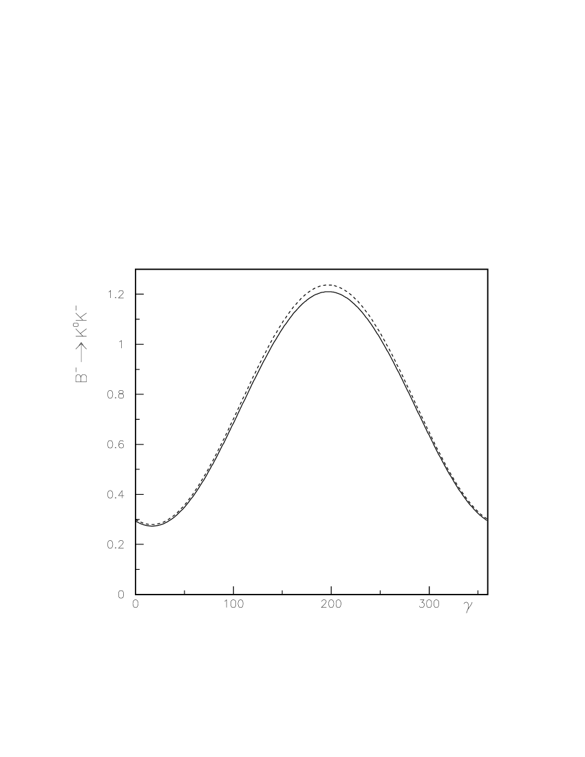
Figure 3: Dependence of the branching ratio on the weak phase $\gamma$ in the $B^{-}\rightarrow K^{0}K^{-}$ channel. The dashed and solid lines correspond to the values obtained with $M_{f}+M_{\alpha_{s}}$ and $M_{f}+M_{\alpha_{s}}+M_{nf}$, respectively.

For comparison, we plot the branching ratios (Br) for these decay modes as a function of $\gamma$ in Fig.1-Fig.3. Eqs.(21)-(23) show that the soft-gluon contributions to the decay amplitudes are much smaller than the factorization parts in $B\rightarrow KK$ decays. The contributions depend on different decay modes. In the case of $\bar{B_{s}}^{0}\rightarrow K^{0}\bar{K}^{0}$, there are only penguin diagram contributions and they come mainly from the factorization and $\alpha_{s}$ correction parts; soft-gluon contribution is suppressed by the order of $10^{-1}$ with respect to the former. The soft-gluon effects make the branching ratio smaller and the results are shown in Fig.1. The dashed and solid curves correspond to the values obtained from $M_{f}+M_{\alpha_{s}}$ and $M_{f}+M_{\alpha_{s}}+M_{nf}$, respectively. In the case of $\bar{B_{s}}^{0}\rightarrow K^{+}K^{-}$, the soft contribution has the same order as the $\alpha_{s}$ correction parts in the tree amplitudes. In the penguin amplitudes, it has the amplitude of order $10^{-9}$, which is smaller than those of factorization and $\alpha_{s}$ correction parts (of order $10^{-7}$). It is shown from Fig.2 that the total branching ratio is suppressed by soft-gluon effects. In the case of $B^{-}\rightarrow K^{0}K^{-}$, the soft-gluon amplitude is of order $10^{-8}$, which is obviously lower than that of the factorization (of order $10^{-6}$) and $\alpha_{s}$ correction (of order $10^{-7}$). Fig.3 show that the total branching ratio is decreased by soft-gluon effects, too.

IV SUMMARY

In this paper, we have analyzed the $B\rightarrow KK$ decays with the soft-gluon corrections by the QCD light-cone sum rules. The soft contributions depend on decay modes, and in most situations they have the amplitudes which are suppressed by the order of $10^{-1}$ or $10^{-2}$ of factorization and $\alpha_{s}$ correction amplitudes. Only in the case of $\bar{B}_{s}^{0}\rightarrow K^{+}K^{-}$, they have the same order amplitude with $\alpha_{s}$ correction parts which is smaller than the factorization amplitude. Our results show that the soft-gluon effects on $B\rightarrow KK$ are small and they always suppress the branching ratio values with 2-3 $\%$ corrections .

References

• (1) A.Khodjamirian, Nucl. Phys. B 605, 558 (2001).
• (2) M. Beneke, G. Buchalla, M. Neubert, C. T. Sachralda, Phys. Rev. Letter. B 83, 1914 (1999); Nucl. Phys. B 591, 313 (2000).
• (3) Wu xiang-Yao, Li Zuo-Hong, Cui Jian-Ying, Huang-Tao, Chin. Phys. Lett. 11, 1596, (2002).
• (4) G. Buchalla, A. J. Buras and M. E. Lautenbacher, Rev. Mod. Phys. 68, 1125 (1996).
• (5) P.Ball, JHEP 9809, 005 (1998).
• (6) Tao Huang, Zuo-Hong Li and Xiang-Yao Wu, Phys. Rev. D 63, 094001 (2001).
• (7) Dong Zhang, Zhen-Jun Xiao, Chong-Sheng Li, Phys. Rev. D 64,014014 (2001)
• (8) M. Beneke, G. Buchalla, M. Neubert, C. T. Sachralda, Nucl. Phys. B 606, 245 (2001). A. Ali, G. Kramer and C. D. Lu, Phys. Rev. D 58, 094009 (1998).