LBNL-51861

In the context of the brane-world scenarios with compactified large extra dimensions, we study the production of the possible massive brane oscillations (branons) in electron-positron colliders. We compute their contribution to the electroweak gauge bosons decay width and to the single-photon and single-Z processes. With LEP-I results and assuming non observation at LEP-II we present exclusion plots for the brane tension $\tau=f^{4}$ and the branon mass $M$. Prospects for the next generation of electron-positron colliders are also considered.

PACS: 11.25Mj, 11.10Lm, 11.15Ex

1 Introduction

In the last years a lot of attention has been paid to the so called brane world or ADD scenarios [1] where the Standard Model particles are confined to live in the world brane and only gravitons are free to move along the $D$ dimensional bulk space (see [2] for recent reviews). The phenomenological consequences of these real or virtual gravitons, described in terms of their corresponding Kaluza-Klein (KK) towers, in colliders or in astrophysical and cosmological scenarios, have been the object of many recent works (see [3] and references therein). However, in addition to the gravitons and the Standard Model (SM) particles, one has to consider in principle the possibility of having also brane oscillations (branons). In fact, it has been shown that these branons or, equivalently, the brane recoil, give rise to an exponential suppression of the couplings of the SM particles and the higher KK modes [4] in such a way that, in the $f\ll M_{F}$ regime (where $\tau=f^{4}$ is the brane tension and $M_{F}$ is the $D$ dimensional fundamental scale of gravity), the most important modes at low energies are the SM particles and the branons. Moreover branons can play a role in the solution of some problems appearing when the flexibility of the brane is not taken into account such as divergent virtual contributions from the KK tower or non-unitary graviton production cross-sections.

The effective action for the SM fields on the brane was obtained in [5]. The introduction of brane fluctuations was done in [6], where the interaction between branons and the SM particles, and the branons self interactions, were obtained including also the possibility of having non-vanishing branon masses due to the non-factorization of the extra dimension space.

The effects of brane recoil on real graviton production have been studied for example in [7], and on virtual gravitons and gauge bosons in [8, 9]. Some constraints from astrophysics on the brane tension were considered in [10] and the direct production of branons in colliders was discussed in [11], for massless branons in both cases.

In this work we are interested in the production rates of massive branons in electron-positron colliders, in order to get bounds on the brane tension and the branon mass in the above mentioned scenario where the brane tension scale $f$ is much smaller that the $D$ dimensional fundamental scale of gravity $M_{F}$. The paper is organized as follows: in Sec. II we define our set up and give the effective action for massive branons. In Sec. III we obtain their couplings to the SM particles and in Sec. IV we discuss the kind of bounds which is possible to set on the brane parameters, namely the number of branons $n$, their mass $M$ and the brane tension scale $f$. Sec. V is devoted to the analysis of the Z invisible width and Sec. VI to the $W$ decay. Direct searches based on single-photon and single-Z processes are considered in Sec. VII, and extended to future linear colliders in Sec VIII. Sec. IX offers the summary and the main conclusions of this work. In addition, the relevant Feynman rules are shown in App. A. In App. B the probability amplitudes are calculated for the relevant processes and in App. C, it is possible to find some two-body phase-space exact integrals which were used in this work. Finally, App. D contains some explicit expressions for the cross sections.

2 The effective action for massive brane fluctuations

We will consider a single-brane model in large extra dimensions. In such model, our four-dimensional space-time $M_{4}$ is embedded in a $D$-dimensional bulk space which, for simplicity, we will assume to be of the form $M_{D}=M_{4}\times B$. The $B$ space is a given N-dimensional compact manifold, so that $D=4+N$. The brane lies along $M_{4}$ and we neglect its contribution to the bulk gravitational field. The coordinates parametrizing the points in $M_{D}$ will be denoted by $(x^{\mu},y^{m})$, where the different indices run as $\mu=0,1,2,3$ and $m=1,2,...,N$. The bulk space $M_{D}$ is endowed with a metric tensor which we will denote by $G_{MN}$, with signature $(+,-,-...-,-)$. For simplicity, we will consider the following ansatz:

$$G_{MN} = \left(\begin{array}[]{cccc}\tilde{g}_{\mu\nu}(x)&0\\ 0&-\tilde{g}^{\prime}_{mn}(y)\end{array}\right).$$ (3)

The position of the brane in the bulk can be parametrized as $Y^{M}=(x^{\mu},Y^{m}(x))$, with $M=0,\dots,3+N$ and where we have chosen the bulk coordinates so that the first four are identified with the space-time brane coordinates $x^{\mu}$. We assume the brane to be created at a certain point in $B$, i.e. $Y^{m}(x)=Y^{m}_{0}$ which corresponds to its ground state.

The induced metric on the brane in such state is given by the four-dimensional components of the bulk space metric, i.e. $g_{\mu\nu}=\tilde{g}_{\mu\nu}=G_{\mu\nu}$. However, when brane excitations are present, the induced metric is given by

$$g_{\mu\nu}=\partial_{\mu}Y^{M}\partial_{\nu}Y^{N}G_{MN}(x,Y(x))=\tilde{g}_{\mu\nu}(x,Y(x))-\partial_{\mu}Y^{m}\partial_{\nu}Y^{n}\tilde{g}^{\prime}_{mn}(Y(x)).$$ (4)

Since the mechanism responsible for the creation of the brane is in principle unknown, we will assume that the brane dynamics can be described by an effective action. Thus, we will consider the most general expression which is invariant under reparametrizations of the brane coordinates. Following the philosophy of the effective Lagrangians technique, we will also organize the action as a series in the number of the derivatives of the induced metric over a dimensional constant, which can be identified with the brane tension scale $f$. From this point of view, to the lowest order in derivatives we find:

$$S_{B}=\int_{M_{4}}d^{4}x\sqrt{g}\left(-f^{4}+\dots\right),$$ (5)

where $d^{4}x\sqrt{g}$ is the volume element of the brane. Notice that this lowest order term is the usual Dirac-Nambu-Goto action. However, in certain circumstances the effect of the higher order terms must be taken into account [12].

In the absence of the 3-brane, the metric (3) possesses an isometry group which we will assume to be of the form $G(M_{D})=G(M_{4})\times G(B)$. If the brane ground state is $Y^{m}(x)=Y^{m}_{0}$, the presence of the brane will break spontaneously all the $B$ isometries, except those that leave the point $Y_{0}$ unchanged. In other words the group $G(B)$ is spontaneously broken down to $H(Y_{0})$, where $H(Y_{0})$ denotes the isotropy group (or little group) of the point $Y_{0}$. Therefore, we can introduce the coset space $K=G(M_{D})/(G(M_{4})\times H(Y_{0}))=G(B)/H(Y_{0})$.

Let $H_{i}$ be the $H(Y_{0})$ generators ($i=1,2,...\;h$), $X_{\alpha}$ ($\alpha=1,2,...\;k=\mbox{dim}\;G(B)-\mbox{dim}\;H$) the broken generators, and $T=(H,X)$ the complete set of generators of $G(B)$. A similar separation can be done with the Killing fields. We will denote $\xi_{i}$ those associated to the $H_{i}$ generators, $\xi_{\alpha}$ those corresponding to $X_{\alpha}$ and by $\xi_{a}(y)$ the complete set of Killing vectors on $B$. As shown in [6], the excitations of the brane along the directions of the broken generators of $B$ correspond to the zero modes and they are parametrized by the Goldstone bosons (branon fields) $\pi^{\alpha}(x)$, which can be understood as coordinates on the coset manifold $K$. When the $B$ space is homogeneous then the coset $K$ is isomorphic to $B$ and the isometries are just translations. In this case the branon fields ($\pi$) can be identified with properly chosen coordinates in the extra space ($Y$).

According to the previous discussion, we can write the induced metric on the brane in terms of branon fields as:

$$g_{\mu\nu}=\tilde{g}_{\mu\nu}(x)-\tilde{g}^{\prime}_{mn}\frac{\partial Y^{m}}{\partial\pi^{\alpha}}\frac{\partial Y^{n}}{\partial\pi^{\beta}}\partial_{\mu}\pi^{\alpha}\partial_{\nu}\pi^{\beta}.$$ (6)

Introducing the tensor $h_{\alpha\beta}(\pi)$ as

$$h_{\alpha\beta}(\pi)=f^{4}\tilde{g}^{\prime}_{mn}(Y(\pi))\frac{\partial Y^{m}}{\partial\pi^{\alpha}}\frac{\partial Y^{n}}{\partial\pi^{\beta}},$$ (7)

we have

$$g_{\mu\nu} = \tilde{g}_{\mu\nu}(x)-\frac{1}{f^{4}}h_{\alpha\beta}(\pi)\partial_{\mu}\pi^{\alpha}\partial_{\nu}\pi^{\beta}.$$ (8)

Branons are massless only if the isometry pattern introduced before is exact. However, in general, the symmetry is only approximately realized and branons will acquire mass. In order to show this mechanism explicitly, let us perturb the four-dimensional components of the background metric and let $\tilde{g}_{\mu\nu}$ depend, not only on the $x$ coordinates, but also on the $y$ ones:

$$G_{MN} = \left(\begin{array}[]{cccc}\tilde{g}_{\mu\nu}(x,y)&0\\ 0&-\tilde{g}^{\prime}_{mn}(y)\end{array}\right).$$ (11)

This has to be done in such a way that the $G(B)$ piece of the full isometry group is explicitly broken. Notice that the breaking of the $G(B)$ group by perturbing only the internal metric $\tilde{g}_{mn}^{\prime}(y)$ does not lead to a mass term for the branons.

In order to calculate the branon mass matrix, we need to know first the ground state around which the brane is fluctuating. With that purpose, we will consider for simplicity the lowest-order action, given by:

$$S_{eff}^{(0)}[\pi] = \int_{M_{4}}d^{4}x{\cal L}^{(0)}=-f^{4}\int_{M_{4}}d^{4}x\sqrt{\tilde{g}(x,Y(x))}$$ (12)

which will have an extremum provided

$$\delta S_{eff}^{(0)}[\pi]=0\Rightarrow\delta\sqrt{\tilde{g}}=\frac{1}{2}\sqrt{\tilde{g}}\tilde{g}^{\mu\nu}\delta\tilde{g}_{\mu\nu}=0\Rightarrow\tilde{g}^{\mu\nu}\partial_{m}\tilde{g}_{\mu\nu}=0,\forall y^{m}.$$ (13)

This is a set of equations whose solution $Y^{m}_{0}(x)$ determines the shape of the brane in its ground state for a given background metric $\tilde{g}_{\mu\nu}$. In addition, the condition for the energy to be minimum requires:

$$\left.\frac{\delta^{2}{\cal L}^{(0)}}{\delta Y^{m}\delta Y^{n}}\right|_{Y=Y_{0}} = \frac{-f^{4}}{4}\sqrt{\tilde{g}}\tilde{g}^{\mu\nu}(\partial_{n}\partial_{m}\tilde{g}_{\mu\nu}-2\tilde{g}^{\rho\sigma}\partial_{n}\tilde{g}_{\nu\sigma}\partial_{m}\tilde{g}_{\mu\rho})<0.$$ (14)

i.e. the eigenvalues of the above matrix should be negative. This implies that the static Lagrangian should have a maximum.

In order to obtain the explicit expression of the branon mass matrix, we expand $\tilde{g}_{\mu\nu}(x,y)$ around $y^{m}=Y^{m}_{0}$ in terms of the $\pi^{\alpha}$ fields:

$$\tilde{g}_{\mu\nu}(x,y) = \tilde{g}_{\mu\nu}(x,Y_{0})+\partial_{m}\tilde{g}_{\mu\nu}(x,Y_{0})(Y^{m}-Y^{m}_{0})$$

$$+ \frac{1}{2}\partial_{m}\partial_{n}\tilde{g}_{\mu\nu}(x,Y_{0})(Y^{m}-Y^{m}_{0})(Y^{n}-Y^{n}_{0})+...$$

$$= \tilde{g}_{\mu\nu}(x,Y_{0})+\frac{1}{f}V_{\alpha\mu\nu}^{(1)}\pi^{\alpha}+\frac{1}{f^{2}}V_{\alpha\beta\mu\nu}^{(2)}\pi^{\alpha}\pi^{\beta}+\frac{1}{f^{3}}V_{\alpha\beta\gamma\mu\nu}^{(3)}\pi^{\alpha}\pi^{\beta}\pi^{\gamma}+\dots$$

The linear term in branon fields is written as:

$$\frac{1}{f}V_{\alpha\mu\nu}^{(1)}=\left.\partial_{m}\tilde{g}_{\mu\nu}(x,y)\right|_{y=Y_{0}}\frac{\xi^{m}_{\alpha}}{kf^{2}},$$ (16)

while the quadratic term takes the general form:

$$\frac{1}{f^{2}}V_{\alpha\beta\mu\nu}^{(2)}=\frac{1}{2}\left.\partial_{m}\tilde{g}_{\mu\nu}(x,y)\right|_{y=Y_{0}}\left.\frac{\partial^{2}Y^{m}}{\partial\pi^{\alpha}\partial\pi^{\beta}}\right|_{\pi=0}+\frac{1}{2}\left.\partial_{m}\partial_{n}\tilde{g}_{\mu\nu}(x,y)\right|_{y=Y_{0}}\frac{\xi^{m}_{\alpha}\xi^{n}_{\beta}}{k^{2}f^{4}}$$ (17)

and we have not written the explicit expression for $V_{\alpha\beta\gamma\mu\nu}^{(3)}$ since it will play no role in the present work. Here, we have used the fact that the action of an element of $G(B)$ on $B$ will map $Y_{0}$ into some other point with coordinates:

$$Y^{m}(x)=Y^{m}(Y_{0},\pi^{\alpha}(x))=Y^{m}_{0}+\frac{1}{kf^{2}}\xi^{m}_{\alpha}(Y_{0})\pi^{\alpha}(x)+{\cal O}(\pi^{2})$$ (18)

where we have set the normalization of the branon and Killing fields with $k^{2}=16\pi/M_{P}^{2}$ being $M_{P}$ the four-dimensional Planck mass. Substituting the above expression back in (8), we get the expansion of the induced metric in branon fields:

$$g_{\mu\nu}=\tilde{g}_{\mu\nu}(x,Y_{0})-\frac{1}{f^{4}}\delta_{\alpha\beta}\partial_{\mu}\pi^{\alpha}\partial_{\nu}\pi^{\beta}+\frac{1}{f}V_{\alpha\mu\nu}^{(1)}\pi^{\alpha}+\frac{1}{f^{2}}V_{\alpha\beta\mu\nu}^{(2)}\pi^{\alpha}\pi^{\beta}+{\cal O}(\pi^{3}).$$ (19)

We have also used the fact that since $\pi^{\alpha}$ must be properly normalized scalar fields, the $Y^{m}$ coordinates should be normal and geodesic in a neighborhood of $Y^{m}_{0}$ and, in particular, they cannot be angular coordinates. This implies that we can write $h_{\alpha\beta}(\pi=0)=\delta_{\alpha\beta}$.

Assuming for concreteness that, in the ground state, the four-dimensional background metric is flat, i.e. $\tilde{g}_{\mu\nu}(x,Y_{0})=\eta_{\mu\nu}$, the appearance of the $V_{\alpha_{1}\alpha_{2}...\alpha_{i}\mu\nu}^{(i)}$ tensors in (2) could break Lorentz invariance, unless they factor out as $V_{\alpha_{1}\alpha_{2}...\alpha_{i}\mu\nu}^{(i)}=M_{\alpha_{1}\alpha_{2}...\alpha_{i}}^{(i)}\eta_{\mu\nu}/(4f^{2})$. With this assumption, the linear term $V_{\alpha\mu\nu}^{(1)}$ vanishes identically due to the condition of minimum for the brane energy (13), and the $M_{\alpha\beta}^{(2)}$ coefficient in the quadratic term can be identified with the branon mass matrix. Thus, in general and for the square root of the metric determinant we find:

$$\sqrt{g}=1-\frac{1}{2f^{4}}\eta^{\mu\nu}\delta_{\alpha\beta}\partial_{\mu}\pi^{\alpha}\partial_{\nu}\pi^{\beta}+\frac{1}{2f^{4}}M_{\alpha\beta}^{(2)}\pi^{\alpha}\pi^{\beta}+...$$ (20)

Notice that this expression requires that both $\partial\pi/f^{2}$ and $M^{2}\pi^{2}/f^{4}$ are small. This includes different types of expansions, such as low-energy expansions with small branon masses compared to $f$, or low-energy expansions with possible large masses and small $\pi/f$ factors.

The different terms in the effective action can be organized according to the number of branon fields:

$$S_{eff}[\pi]=S_{eff}^{(0)}[\pi]+S_{eff}^{(2)}[\pi]+...$$ (21)

where the zeroth order term is just a constant. The free action contains the terms with two branons:

$$S_{eff}^{(2)}[\pi]=\frac{1}{2}\int_{M_{4}}d^{4}x(\delta_{\alpha\beta}\partial_{\mu}\pi^{\alpha}\partial^{\mu}\pi^{\beta}-M^{2}_{\alpha\beta}\pi^{\alpha}\pi^{\beta}).$$ (22)

3 Couplings to the Standard Model fields

As we have shown in the previous sections, the induced metric on the brane depends on both the four-dimensional bulk metric components $\tilde{g}_{\mu\nu}$ and the branon fields $\pi^{\alpha}$. As noticed in [8], in the limit in which gravity decouples $M_{F}\rightarrow\infty$, the branon fields still survive. This implies that their effects can be studied independently of gravity. With that purpose, in the following, we will consider their couplings to the Standard Model fields in the absence of gravitational background field i.e. $\tilde{g}_{\mu\nu}=\eta_{\mu\nu}$. In order to obtain the general couplings, one can proceed as in [6], where the action on the brane, which is basically the SM action defined on a curved space-time $M_{4}$, is expanded in branon fields through the induced metric. For example, the complete action, including terms with two branons, contains the SM term, the kinetic term for the branons and the interaction terms between the SM particles and the branons:

$$S_{B} = \int_{M_{4}}d^{4}x\sqrt{g}[-f^{4}+{\cal L}_{SM}(g_{\mu\nu})]$$ (23)

$$= \int_{M_{4}}d^{4}x\left[-f^{4}+{\cal L}_{SM}(\eta_{\mu\nu})+\frac{1}{2}\eta^{\mu\nu}\delta_{\alpha\beta}\partial_{\mu}\pi^{\alpha}\partial_{\nu}\pi^{\beta}-\frac{1}{2}M^{2}_{\alpha\beta}\pi^{\alpha}\pi^{\beta}\right.$$

$$+ \left.\frac{1}{8f^{4}}(4\delta_{\alpha\beta}\partial_{\mu}\pi^{\alpha}\partial_{\nu}\pi^{\beta}-M^{2}_{\alpha\beta}\pi^{\alpha}\pi^{\beta}\eta_{\mu\nu})T^{\mu\nu}_{SM}(\eta_{\mu\nu})\right]+{\cal O}(\pi^{3}).$$

where $T^{\mu\nu}_{SM}(\eta_{\mu\nu})$ is the conserved energy-momentum tensor of the Standard Model evaluated in the background metric:

$$T^{\mu\nu}_{SM}=-\left.\left(\tilde{g}^{\mu\nu}{\cal L}_{SM}+2\frac{\delta{\cal L}_{SM}}{\delta\tilde{g}_{\mu\nu}}\right)\right|_{\tilde{g}_{\mu\nu}=\eta_{\mu\nu}}$$ (24)

It is interesting to note that there is no single branon interactions which, as commented above would be related to Lorentz invariance breaking. In addition the quadratic expression in (23) is valid for any internal $B$ space, regardless of the particular form of the metric $\tilde{g}^{\prime}_{mn}$. In fact, the form of the couplings only depends on the number of branon fields, their mass and the brane tension. The dependence on the geometry of the extra dimensions will appear only at higher orders.

Let us give the results for the different kinds of fields. The corresponding Feynman rules can be found in Appendix A (we will follow the notation in [6]):

Scalars

For a complex scalar field $\Phi$ with mass $m_{\Phi}$ in a certain representation of a gauge group with generators $T^{a}$, the Lagrangian is given by:

$${\cal{L}}_{S}=(D_{\mu}\Phi)^{\dagger}D^{\mu}\Phi-m_{\Phi}^{2}\Phi^{\dagger}\Phi,$$ (25)

whose energy-momentum tensor is given by:

$$T^{\mu\nu}_{S}=-\eta^{\mu\nu}((D_{\rho}\Phi)^{\dagger}D^{\rho}\Phi-m_{\Phi}^{2}\Phi^{\dagger}\Phi)+(D^{\mu}\Phi)^{\dagger}D^{\nu}\Phi+(D^{\nu}\Phi)^{\dagger}D^{\mu}\Phi$$ (26)

where the gauge covariant derivative has the usual form $D_{\mu}=\partial_{\mu}-hA^{a}_{\mu}T^{a}$. From this expression we find the Feynman rules for the following types of vertices: $\pi\pi\Phi^{\dagger}\Phi$, $\pi\pi\Phi^{\dagger}\Phi A$ and $\pi\pi\Phi^{\dagger}\Phi AA$.

Fermions

The Lagrangian for a Dirac fermion field with mass $m_{\psi}$ reads:

$${\cal{L}}_{f}=\bar{\psi}(i\gamma^{\mu}D_{\mu}-m_{\psi})\psi,$$ (27)

and its associated energy-momentum tensor is:

$$T^{\mu\nu}_{F} = \frac{i}{4}\{\bar{\psi}(\gamma^{\mu}D^{\nu}+\gamma^{\nu}D^{\mu})\psi\ -(D^{\nu}\bar{\psi}\gamma^{\mu}+D^{\mu}\bar{\psi}\gamma^{\nu})\psi\}$$ (28)

$$- \frac{1}{2}\eta^{\mu\nu}\{i(\bar{\psi}\gamma^{\rho}D_{\rho}-D_{\rho}\bar{\psi}\gamma^{\rho})\psi-2m_{\psi}\bar{\psi}\psi\}.$$

where again we assume the fermion field $\psi$ to be in a certain representation of a gauge group with generators $T^{a}$, and the covariant derivatives are defined as $D_{\mu}=\partial_{\mu}-hT^{a}A^{a}_{\mu}(c_{V}(a)-c_{A}(a)\gamma_{5})$, where, in general, the vector and axial couplings could be different. The Feynman rules will contain the following types of vertices: $\pi\pi\bar{\psi}\psi$ and $\pi\pi\bar{\psi}\psi A$.

Gauge bosons

For the Yang-Mills action on the brane we can follow similar steps. The Lagrangian is given by:

$${\cal{L}}_{A}=-\frac{1}{4}F^{a\,\mu\nu}F^{a}_{\mu\nu}+{\cal{L}}_{FP}$$ (29)

where:

$$F^{a}_{\mu\nu}=\partial_{\mu}A^{a}_{\nu}-\partial_{\nu}A^{a}_{\mu}-hC^{abc}A^{b}_{\mu}A^{c}_{\nu},$$ (30)

${\cal{L}}_{FP}$ is the Fadeev-Popov Lagrangian, which includes the gauge fixing and the ghost terms. The gauge symmetry can be spontaneously broken in such a way that the gauge fields acquire masses $M_{a}$ through their couplings to the scalar sector (25). In that case, a renormalizable gauge will be used in the calculations. It is interesting to notice that the metric used in the gauge fixing term could be either the induced metric or the flat background metric. Both choices give rise to valid gauge-fixing expressions. The second one is however simpler because it does not introduce new couplings between gauge or Goldstone bosons fields and branons. The same criterion has to be taken for the ghost Lagrangian, which will not be studied here since we are only interested in the tree-level analysis.

The energy-momentum tensor takes the form:

$$T^{\mu\nu}_{A} = F^{a}_{\rho\sigma}F^{a}_{\lambda\theta}(\eta^{\sigma\lambda}\eta^{\rho\mu}\eta^{\theta\nu}+\frac{1}{4}\eta^{\rho\lambda}\eta^{\sigma\theta}\eta^{\mu\nu})+T^{\mu\nu}_{FP}$$ (31)

and from this interaction action, one finds the Feynman rules for vertices like $\pi\pi AA$, $\pi\pi AAA$ and $\pi\pi AAAA$

We see that in all these vertices, branons always interact by pairs with the SM matter fields. In addition, due to their geometric origin, those interactions are very similar to the gravitational ones since the $\pi$ fields couple to all the matter fields through the energy-momentum tensor and with the same strength, which is suppressed by a $f^{4}$ factor. In fact, branons couple as gravitons do, with the following identification:

$$h_{\mu\nu} \longrightarrow -\frac{1}{kf^{4}}h_{\alpha\beta}(\pi)\partial_{\mu}\pi^{\alpha}\partial_{\nu}\pi^{\beta},$$ (32)

where $h_{\mu\nu}$ is the graviton field in linearized gravity.

4 Constraining brane-world models

In the brane-world scenario, with $f\ll M_{F}$, the relevant low-energy excitations on the brane correspond to the branons rather than to the Kaluza-Klein graviton excitations. In such case, and provided the energy scale of present accelerators is well below both the fundamental scale of gravity $M_{F}$ and the brane tension scale $f$, but is large compared to the branon mass $M$, such branon fields will be produced in the collision of SM particles. Moreover, the calculation of the corresponding production cross-sections could be performed by using the effective theory described in the previous section.

In principle, there would be new physics related to both the KK gravitons and the branons, but the dependence on $f$ in each case is completely different. For example, the behavior of typical cross sections for missing energy processes, i.e. KK graviton and branon production processes, becomes large for both small and large values of the brane tension $f$ [10]. The cross section for a small value of $f$ is governed by the branon production process, while for a large value, the KK gravitons production rate dominates. Therefore if the brane tension scale is smaller than the fundamental gravitational one, then the first indications of extra dimensions would be given by the production of branons. This would allow us to measure the brane tension and the branon mass or, if branons are not found, at least to set bounds on such parameters.

The effective couplings introduced in the previous section provide the necessary tools to compute the cross sections and the expected rates of new exotic events in terms of $f$ and the branons masses only. In fact, with a rotation in the coset space $K$, the branon mass matrix takes a diagonal form. We will assume that there are $n$ branons with the same mass $M$. If the branons masses are similar this would be a good approximation. In the opposite case, with very different masses, we could neglect the heavier fields and consider only the production of light branons. In these simple cases, all the cross sections will be parametrized by three unknown parameters:

$n$: number of branons.

$M$: mass of the branons.

$f$: brane tension scale.

In the following, we will compare the data coming from LEP with the predicted cross section for different processes in which we expect high sensitivity to new physics. In particular we will concentrate on the branon contribution to the invisible width of the Z boson, to the decay rate of the $W^{\pm}$ bosons and to direct searches with single-photon and single-Z vertices. This will allow us to set bounds on certain combinations of the above parameters.

5 Bounds from the Z invisible width

In the Standard Model, the full decay width of the Z boson has three types of contributions, coming from charged leptons, hadrons and neutrinos respectively. The third one corresponds to the so called invisible width, since neutrinos escape without producing any signal in the detectors. In principle, physics beyond the SM could also give rise to invisible decays of Z and therefore to deviations with respect to the SM predictions.

The precision measurements done mostly at LEP-I set stringent limits on the Z invisible decay width, which can be translated into strong bounds on the new channels contributing to such process. In fact in the following, we will show how it is possible to get lower bounds on the brane tension $f$ coming from light branons ($M<M_{Z}/2$) in which the Z could decay. Since branons are stable and chargeless particles, they would also avoid detection.

In this section we calculate the first order contribution from branons to this width, which is given by the decay of Z into two branons and two neutrinos:

$\Gamma_{Z}^{b}$: $Z\longrightarrow\bar{\nu}(p_{1}),\nu(p_{2})\pi(k_{1}),\pi(k_{2})$

We use the expression for the probability amplitudes in Appendix B Eq.(67) calculated with the Feynman rules given in Appendix A. We integrate over the branon two-body phase space making use of the formulae in Appendix C. The result is averaged over the three Z polarizations. In addition, such expression should be divided by two because the outgoing branons are indistinguishable. Thus we get:

$$\frac{d\Gamma_{Z}^{b}}{d^{3}\overrightarrow{p_{1}}d^{3}\overrightarrow{p_{2}}} = \frac{|h|^{2}}{4\pi}\frac{2M_{Z}n}{61440f^{8}3\pi^{6}t^{2}u^{2}(M_{Z}^{2}-t)(M_{Z}^{2}-u)(M_{Z}^{2}-s)^{2}}$$ (33)

$$\sqrt{1-\frac{4M^{2}}{k^{2}}}\{20M^{2}M_{Z}^{2}(2k^{2}-5M^{2})t^{2}u^{2}(M_{Z}^{2}(2s-k^{2})+tu)$$

$$+ (k^{2}-4M^{2})^{2}\{stu(s(k^{2}+M_{Z}^{2})+4tu)(2s(k^{2}+M_{Z}^{2})+t^{2}+u^{2})$$

$$+ (t^{2}+u^{2})(2s+2k^{2}+M_{Z}^{2})M_{Z}^{8}$$

$$- [6s(t^{3}+u^{3})+6s^{2}(t^{2}+u^{2}-tu)+3tu(t-u)^{2}+t^{4}+u^{4}]M_{Z}^{6}$$

$$+ M_{Z}^{4}[2s^{3}(2(t^{2}+u^{2})-5tu)+2s^{2}(3(t^{3}+u^{3})-5tu(t+u))$$

$$+ s(2(t^{4}+u^{4})+tu(t^{2}+u^{2}-8tu))+tu(t^{3}+u^{3}-7tu(t+u))]$$

$$- M_{Z}^{2}[s^{4}(t-u)^{2}-8t^{3}u^{3}+2s^{3}(t^{3}+u^{3}-2tu(t+u))$$

$$+ 2stu(t^{3}+u^{3}-3tu(t+u))$$

$$+ s^{2}(t^{4}+u^{4}+tu(t^{2}+u^{2}-14tu))]\}\}$$

where we have used equations (67) with $c_{V}=c_{A}=1$, $M_{a}=M_{Z}$ and the coupling constant $h=g/(4\cos\theta_{W})$, with $\theta_{W}$ the Weinberg angle. We have also made use of the Mandelstam variables: $s\equiv(p_{1}+p_{2})^{2}$, $t\equiv(p_{1}-q)^{2}$, $u\equiv(p_{2}-q)^{2}$ and $k^{2}\equiv(k_{1}+k_{2})^{2}$, although only three of them are independent because $s+t+u=k^{2}+M_{Z}^{2}$.

We can also compute the above differential cross section in terms of (non-covariant) variables with a more physical interpretation, namely, the energies of the outgoing neutrino and antineutrino, $p_{1}^{0}\equiv E_{1}$ and $p_{2}^{0}\equiv E_{2}$ respectively, and the angle between their three-momenta $\theta$. In terms of these variables we have:

$$s = 2p_{1}^{0}p_{2}^{0}(1-\cos\theta),$$

$$t = M_{Z}(M_{Z}-2p_{1}^{0}),$$

$$u = M_{Z}(M_{Z}-2p_{2}^{0}),$$ (34)

The total width is calculated by integrating the above expression with respect to the three variables within the following kinematic limits:

$$p_{1}^{0} \in I_{1}\equiv[0,\frac{M_{Z}^{2}-4M^{2}}{2M_{Z}}],$$ (35)

$$p_{2}^{0} \in I_{2}\equiv[0,\frac{M_{Z}(M_{Z}-2p_{1}^{0})-4M^{2}}{2(M_{Z}-(1-\cos\theta)p_{1}^{0})}],$$

$$\cos\theta \in I_{0}\equiv[-1,1].$$

The final result, depending on the three undetermined parameters reads:

$$\Gamma_{Z}^{b}(n,f,M)=\int_{I_{0}\times I_{1}\times I_{2}}\frac{d\Gamma_{Z}^{b}}{dp_{1}^{0}dp_{2}^{0}d\cos\theta}dp_{1}^{0}dp_{2}^{0}d\cos\theta.$$ (36)

The integration over the rest of angles has been done immediately because the decay rate does not depend of them. It is interesting to note that the dependence on the number of branons $n$ and brane tension $f$ factorizes, and only the dependence on $M$ is non-trivial:

$$\Gamma_{Z}^{b}(n,f,M)=\frac{nM_{Z}^{9}}{f^{8}}\times\Pi(M/M_{Z})$$ (37)

where $\Pi(x)$ is a dimensionless function, which depends on a single dimensionless variable, and which can be easily calculated from (36). For example, for massless branons a numerical integration gives:

$$\Gamma_{Z}^{b}(n,f,0)=\frac{nM_{Z}^{9}}{f^{8}}\times 6.15\times 10^{-13}.$$ (38)

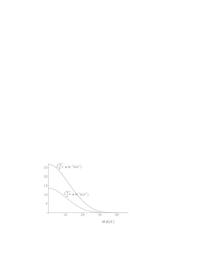
Figure 1: $W^{\pm}$ and Z widths as a function of the branon mass. Both plots correspond to a single channel. We have extracted the dependence on the brane tension and the number of branons in the factor $f^{8}/n$.

To show the dependence on the branon mass, we plot in the Figure 1, $\Gamma_{Z}^{b}(n,f,M)f^{8}/n$ against $M$. Finally, to get the total Z invisible width into branons, we have to multiply by a factor of 3 because there are three different neutrino families.

The key observation is that at the 95$\%$ confidence level, the variation of the Z invisible width cannot be larger than 2.0 MeV [13], i.e., the contribution from new physics satifies:

$$\Gamma_{Z}^{new}(n,f,M)\,<\,2.0\,\mbox{MeV},$$ (39)

It is then possible to find bounds for the different brane parameters just imposing the above limit on Eq.(37). For example, if branons are massless, the bound on $f$ depends only on the number of branons:

$$f\,>\,11.9\,n^{1/8}\,\mbox{GeV}.$$ (40)

On the other hand, in the case of one branon, we show the exclusion plot in the $f-M$ plane (see Figure 2).

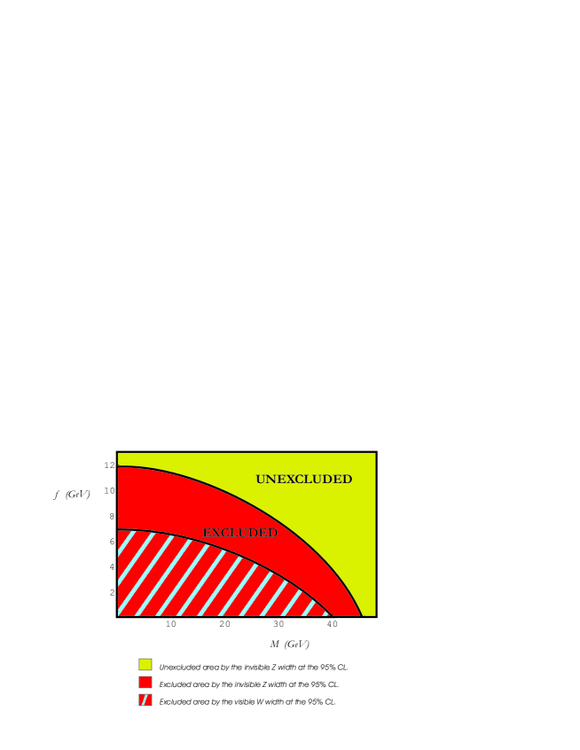
Figure 2: Exclusion plot in the $f-M$ plane for single-branon models from LEP-I data. The dark area is excluded by the measurement of the Z invisible width and the striped region is excluded by the measurement of the visible $W^{\pm}$ decay width.

6 Bounds from $W^{\pm}$ decay

There are mainly two channels contributing to this process. First, the decay of $W^{\pm}$ into two branons and two leptons:

$\Gamma_{W}^{b}$: $W^{-}\longrightarrow l^{-}(p_{1}),\bar{\nu}(p_{2}),\pi(k_{1}),\pi(k_{2})$

Such leptons can be an electron and an electron antineutrino for the $W^{-}$ decay, their antiparticles for $W^{+}$, or the analogue pairs of leptons in the rest of families. The results of the different decay rates agree in the limit in which the lepton masses are negligible. In fact this is a good approximation since the typical energy carried by the of outgoing particles will be comparable to the $W^{\pm}$ mass which is much larger than the leptons masses.

Second, we have the $W^{\pm}$ decay into two branons and a quark-antiquark pair:

$W\longrightarrow q(p_{1}),\bar{q}(p_{2}),\pi(k_{1}),\pi(k_{2})$

In principle there should be also a channel including gluons in the final state, however in the SM, such channel is suppressed by a coefficient $\alpha_{S}(M_{W})/\pi=0.04$ and for that reason we will also ignore it in the present case. In any case, the result we will obtain will be a strict lower bound to the true decay width into branons.

The calculation is totally similar to that of the Z decay and for that reason we will not repeat it here. The expressions for the Z decay in (33) are also valid for the $W^{\pm}$, the only changes, apart from the the different gauge-boson mass, are the $W^{\pm}$ couplings to leptons and quarks. Thus, in this case we have: $M_{a}=M_{W}$, $c_{V}=c_{A}=1$, $h=g/(2\sqrt{2})$ for leptons and $h=V_{ij}g/(2\sqrt{2})$ for quarks where $V_{ij}$ is the Cabbibo-Kobayashi-Maskawa (CKM) matrix element with $i=u,c,t$ and $j=d,s,b$. The differential decay rate has the same form as in the Z case, which is written again in terms of the energy of the two leptons or the quark-antiquark pair $p_{1}^{0}$, $p_{2}^{0}$ and the angle between their three momenta that we denote by $\theta$. Thus the corresponding Mandelstam variables are obtained from (34) just replacing $M_{Z}\rightarrow M_{W}$ The total integration over the leptons or quarks phase-space has to be done in a numerical form, with the analogous limits to those in (5) again replacing the gauge bosons masses.

The final result $\Gamma_{W}^{b}(n,f,M)$ depends on the three unknown parameters and is obtained from the differential rate by using the analogue expression to (36). We see that once again, the dependence on $n$ and $f$ factorizes, and the dependence on $M$ enters through the same dimensionless function $\Pi(x)$. Thus we can write for the leptonic decay:

$$\Gamma_{W}^{b}(n,f,M)=2\cos^{2}\theta_{W}\frac{nM_{W}^{9}}{f^{8}}\times\Pi(M/M_{W}).$$ (41)

For massless branons we obtain by numerical integration:

$$\Gamma_{W}^{b}(n,f,0)=\frac{nM_{W}^{9}}{f^{8}}\times 9.56\times 10^{-13}.$$ (42)

The results in the case of quarks can be obtained in a straightforward way from the leptonic one just multiplying by the modulus squared of the corresponding CKM matrix element.

To show the dependence on the branon mass, we have plotted $\Gamma_{W}^{b}f^{8}/n$ against the branon mass $M$ in Figure 1.

The most important difference with respect to the Z analysis arises from the experimental constraint on the $W^{\pm}$ width coming from new physics. In this case, the decay is visible and, for example, if the final decay products contain $e^{-}$ and $\bar{\nu}_{e}$, the process with branons could give a signal similar to the following Standard Model process: $\Gamma_{W}^{SM}$: $W^{-}\longrightarrow e^{-}(p_{1}),\bar{\nu}_{e}(p_{2}),\nu_{\tau}(p_{3}),\bar{\nu}_{\tau}(p_{4})$, in which, the $W^{-}$ decays into a $\tau^{-}$ and a $\bar{\nu}_{\tau}$, and then the $\tau^{-}$ decays finally into an $e^{-}$, $\bar{\nu}_{e}$ and $\nu_{\tau}$.

The behaviour of the $W^{\pm}$ decay width in terms of the visible lepton energy $E_{l}$ is plotted in Figure 3 for different branon masses.

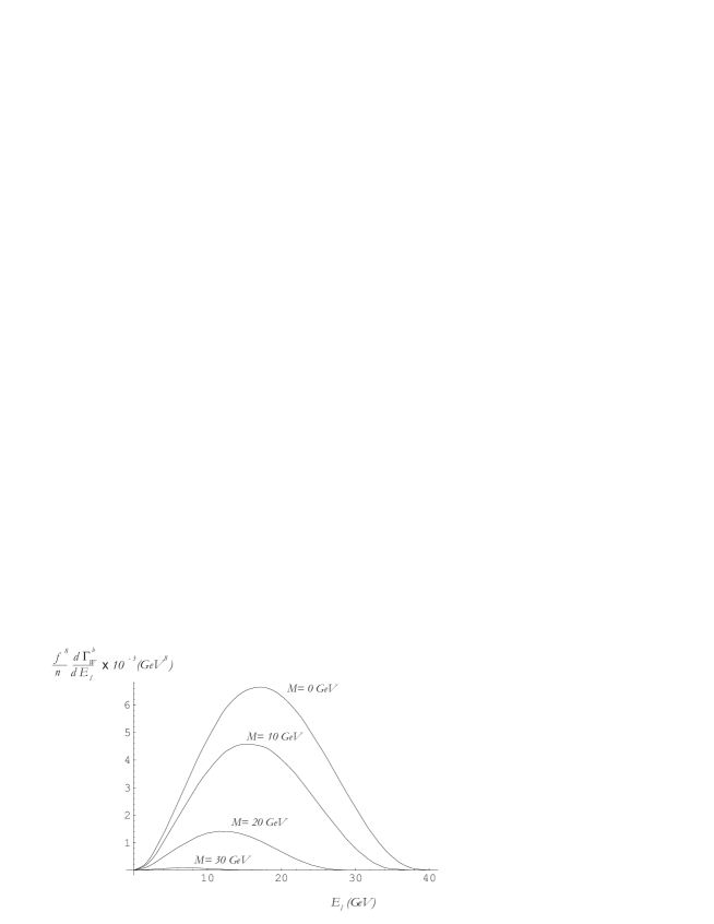
Figure 3: Behaviour of the $W^{\pm}$ decay width in terms of the visible lepton energy $E_{l}$ for different branon masses.

However in this work, we are only interested in the constraints on the theory parameters coming from the total $W^{\pm}$ width. The total leptonic decay is obtained multiplying (41) by a factor of 3, because there are three different kinds of processes corresponding to the three leptonic families. On the other hand, to calculate the hadronic decay we have to multiply by:

$$3\sum_{i=u,\,c\,;j=d,\,s,\,b}|V_{ij}|^{2}=6.117\pm 0.075,$$ (43)

where the factor of 3 comes from the numbers of colors and the sum is extended to the six CKM matrix elements which do not involve the top quark. The numerical result is taken from the combined LEP measurement of $Br(W\longrightarrow q\bar{q})$ [14]. The above approximation assumes that the mass of these five quarks is neglected when compared to the typical energy of the process ($M_{W}$), and the top contribution is neglected because of its large mass. We can thus estimate the total $W^{\pm}$ width just multiplying by $3+6.12$ the result in (41).

In order to get bounds on the contribution from new physics to the $W^{\pm}$ width, $\Gamma_{W}^{new}$, we take into account the uncertainties on the experimental measurement of the visible W width: $\Gamma_{W}^{LEP}=2.150\pm 0.091$ GeV [13], and the uncertainties in the SM calculation: $\Gamma_{W}^{SM}=2.093\pm 0.003$ GeV [14]. So that for the total allowed variation in the visible $W^{\pm}$ width we obtain at the $95\%$ confidence level:

$$\Gamma_{W}^{new}(n,f,M)\,<\,(\Gamma_{W}^{LEP}-\Gamma_{W}^{SM})+2\Delta\Gamma_{W}^{LEP}=240\,\mbox{MeV},$$ (44)

This limit translates into the following one for massless branons:

$$f\,>\,6.9\,n^{1/8}\,\mbox{GeV}.$$ (45)

The exclusion regions as a function of the variables $f$ and $M$ are shown in Figure 2 for the single branon case.

7 Branon bounds from direct searches

7.1 Cross section with a generic gauge boson

In this section we present the cross section of the process:

$$\sigma_{A}:\bar{\psi}(p_{1}),\psi(p_{2})\longrightarrow\pi(k_{1}),\pi(k_{2}),A^{a}_{\mu}(q)$$ (46)

The initial particles can be either leptons or quarks, although we will be mainly interested in the $e^{+}e^{-}$ case. There are three final particles, one arbitrary gauge boson (either Z or $\gamma$) together with the two branons. We are interested in the differential cross section with respect to the gauge boson phase-space parameters, i.e. energy and scattering angle.

We have integrated over the two-body phase space of branons. The probabilities are calculated as usual by doing the square of the amplitude module given in (66). We have also averaged over the spin of the initial particles and summed over polarizations of the outgoing boson. The probability has to be divided by two because the outgoing branons are indistinguishable.

We define the invariants: $s\equiv(p_{1}+p_{2})^{2}$, $t\equiv(p_{1}-q)^{2}$,$u\equiv(p_{2}-q)^{2}$ and $k^{2}\equiv(k_{1}+k_{2})^{2}$. Again only three of them are independent because $s+t+u=k^{2}+M_{a}^{2}$ ($M_{a}$ is the gauge boson mass and we are neglecting the fermion masses). In the CM system the probability should be divided by $2p_{1}^{0}2p_{2}^{0}|v_{1}-v_{2}|=2s$.

Again we can change to more physical variables, namely, the energy fraction of the emitted gauge boson $x=2q_{0}/\sqrt{s}$ and the scattering angle $\theta$. Thus we get:

$$t = -\sqrt{s}(q_{0}-|\overrightarrow{q}|\cos(\theta))+M_{a}^{2}$$

$$u = -\sqrt{s}(q_{0}+|\overrightarrow{q}|\cos(\theta))+M_{a}^{2}$$

$$k^{2} = s(1-x)+M_{a}^{2}$$ (47)

$$q_{0} = \frac{x\sqrt{s}}{2}$$

$$|\overrightarrow{q}| = \frac{1}{2}\sqrt{sx^{2}-4M_{a}^{2}}$$

and the phase-space volume takes the form:

$$\frac{d^{3}q}{2q_{0}(2\pi)^{3}} = \frac{dk^{2}dtd\phi}{4s(2\pi)^{3}}=\frac{dxd(\cos\theta)d\phi}{8(2\pi)^{3}}\sqrt{(sx)^{2}-4sM_{a}^{2}}.$$ (48)

Therefore, for $M_{a}\neq 0$ and arbitrary $c_{V}$ and $c_{A}$ parameters, we have:

$$\frac{d\sigma_{A}}{dxd\cos\theta} = \frac{|h|^{2}}{4\pi}\frac{(c_{V}^{2}+c_{A}^{2})n}{122880f^{8}\pi^{2}(s-M_{a}^{2})^{2}}\sqrt{1-\frac{4M^{2}}{s(1-x)+M_{a}^{2}}}$$

$$\sqrt{s(sx^{2}-4M_{a}^{2})}\{5M^{2}M_{a}^{2}(2(s(1-x)+M_{a}^{2})-5M^{2})$$

$$\{8M_{a}^{2}+(sx^{2}-4M_{a}^{2})\sin^{2}\theta\}$$

$$+ \frac{2(s(1-x)+M_{a}^{2}-4M^{2})^{2}}{(4M_{a}^{2}(M_{a}^{2}+s(1-x))+s(sx^{2}-4M_{a}^{2})\sin^{2}\theta)^{2}}$$

$$\{16M_{a}^{2}(s(1-x)+M_{a}^{2})^{2}[10M_{a}^{6}+M_{a}^{4}s(9-5x)$$

$$+ 2M_{a}^{2}s^{2}(4-3x+x^{2})+s^{3}(1-x)]$$

$$- 2[40M_{a}^{12}-2M_{a}^{10}s(-112+40x+5x^{2})$$

$$+ 4M_{a}^{8}s^{2}(78-70x-3x^{2}+5x^{3})+s^{6}x^{2}(-2+4x-3x^{2}+x^{3})$$

$$+ M_{a}^{6}s^{3}(216-272x+6x^{2}+66x^{3}-11x^{4})$$

$$+ M_{a}^{4}s^{4}(96-184x+62x^{2}+44x^{3}-21x^{4}+x^{5})$$

$$+ M_{a}^{2}s^{5}(8-16x-12x^{2}+42x^{3}-29x^{4}+6x^{5})]\sin^{2}\theta$$

$$+ s(sx^{2}-4M_{a}^{2})^{2}[7M_{a}^{6}+M_{a}^{4}s(17-7x)+M_{a}^{2}s^{2}(1-2x)$$

$$+ s^{3}(3(1-x)+2x^{2})]\sin^{4}\theta-s^{2}(sx^{2}-4M_{a}^{2})^{3}(s-M_{a}^{2})\sin^{6}\theta\}\}.$$

Notice that this expression is also applicable to quark-antiquark collisions just by choosing the appropriate couplings ($c_{V}$ and $c_{A}$ parameters together with $h$).

Also, for certain processes it is interesting to calculate the cross sections without summing over the polarizations ($\epsilon_{\mu}^{a}$) of the outgoing gauge boson. Again we consider the case $M_{a}\neq 0$ and arbitrary $c_{V}$ and $c_{A}$ parameters. The results can be found in Appendix D for longitudinal (76) and transverse (77) polarizations. It is interesting to note that the longitudinal cross secction vanishes in the limit in which the gauge boson mass goes to zero. Therefore, the total cross section (including the three polarizations) in the limit $M_{a}\longrightarrow 0$ has the same form as the total cross section for a massless gauge field ($M_{a}=0$), and it reads:

$$\frac{d\sigma_{A}}{dxd\cos\theta} = \frac{|h|^{2}}{4\pi}\frac{s(c_{V}^{2}+c_{A}^{2})(s(1-x)-4M^{2})^{2}n}{61440f^{8}\pi^{2}}\sqrt{1-\frac{4M^{2}}{s(1-x)}}$$

$$\left[x(3-3x+2x^{2})-x^{3}\sin^{2}\theta+\frac{2(1-x)(1+(1-x)^{2})}{x\sin^{2}\theta}\right]$$

As expected, the cross section is divergent for collinear outgoing boson ($\theta=0$) and also for a soft ($x=0$) massless gauge boson.

7.2 Bounds from single-photon processes

The differential cross section obtained in the previous section could be used in direct searches of branons in colliders. In this section we are going to calculate the contribution to the total cross section of processes involving a single photon in the final state. This will allow us to obtain new bounds on $M$ and $f$ assuming non observation at LEP-II.

To perform the angular integration over the polar angle $\cos\theta$ in (7.1), it is necessary to take into account the angular range covered by the detector $\cos\theta\in[-d,d]$. Thus we get:

$$\frac{d\sigma_{\gamma}}{dx} = \frac{|h|^{2}}{4\pi}\frac{s(c_{V}^{2}+c_{A}^{2})(s(1-x)-4M^{2})^{2}n}{184320\,f^{8}\,{\pi}^{2}\,x}\sqrt{1-\frac{4M^{2}}{s(1-x)}}$$

$$\left(2\,d\,x^{2}\,\left(9-9\,x+\left(3+d^{2}\right)\,x^{2}\right)\right.$$

$$+ \left.3\,\left(-2+4\,x-3\,x^{2}+x^{3}\right)\,\log\left(\frac{{\left(1-d\right)}^{2}}{{\left(1+d\right)}^{2}}\right)\right).$$

where $h=e$, $c_{V}=1$ and $c_{A}=0$.

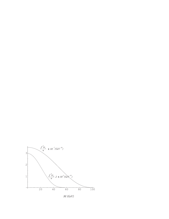
Figure 4: Total cross sections for single-photon and single-Z processes as a function of the branon mass. The dependence on the brane tension and the number of branons has been factorized out in the $f^{8}/n$ coefficient.

The integration in the $x$ variable is done within the following limits $x\in[E_{m}/(2\sqrt{s}),1-4M^{2}/s]$. The upper bound is fixed by kinematical constraints, but the lower one ($X=E_{m}/2\sqrt{s}$), imposing a minimum energy for the photons ($E_{m}$), depends on specific experimental conditions (trigger, noise, backgrounds, …). To perform the numerical study we take $d=0.96$ and $E_{m}=5$ GeV, which correspond to the typical boundary conditions of one of the LEP experiments (see [15]). We will also use $\sqrt{s}=206$ GeV to do the calculations. Although the maximum centre-of-mass energy was close to 209 GeV, most of the data at LEP-II taken in the last year of running were collected in the range between 205 and 207 GeV [13].

The total cross section can be calculated analytically, although it will not be shown here since the final expression is quite long. The result for massless branons (M=0) is much simpler, being just proportional to $s^{3}$:

$$\sigma_{\gamma}(M=0) = \frac{nA_{\gamma}s^{3}}{f^{8}}.$$ (51)

where the constant depends on the detection limits as follows:

$$A_{\gamma} = \frac{-\alpha_{EM}}{11059200\,{\pi}^{2}}\left[\,\left[2\,d\,{\left(-1+X\right)}^{3}\,[30\,\left(1+3\,X-3\,X^{2}+X^{3}\right)\right.\right.$$ (52)

$$+ \left.d^{2}\,\left(1+3\,X+6\,X^{2}+10\,X^{3}\right)\right]+3\,\log\left(\frac{{\left(d-1\right)}^{2}}{{\left(1+d\right)}^{2}}\right)\left(-247+480\,X\right.$$

$$- \,\left.\left.\left.390\,X^{2}+220\,X^{3}-75\,X^{4}+12\,X^{5}-120\,\log(X)\right)\right]\right]$$

with $\alpha_{EM}=e^{2}/(4\pi)$.

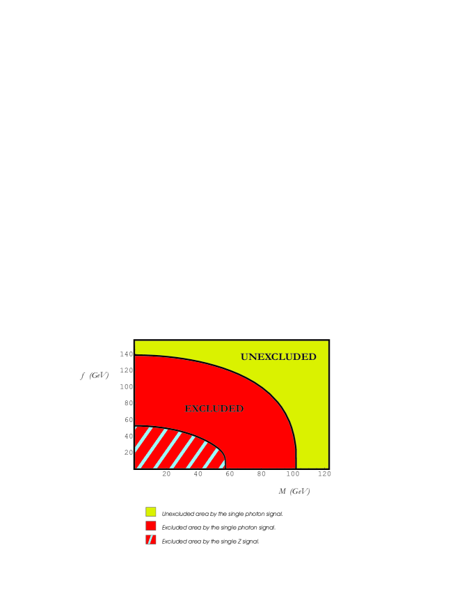
Figure 5: Exclusion regions in the $f-M$ plane coming from single-photon events (dark region) and single-Z processes (striped area), using LEP-II data.

For the limits mentioned before we get $A_{\gamma}=4.54\times 10^{-7}$. The branon mass dependence of the total cross section is plotted in Figure 4.

To obtain the bound on the theory parameters, we can consider the limit on the total cross section coming from new physics which could be added to the single photon channel without being detected. For LEP-II, this limit is approximately $\sigma_{new}\simeq 0.1$ pb, which is the typical experimental sensitivity observed in LEP searches [16]. The result for one branon assuming no observation is plotted in Figure 5. Thus the interior area limited by the bound curve is potentially excluded by the LEP-II experiment. In the case of massless branons, the limit depending on the number of branons reads:

$$f\geq 138n^{1/8}\mbox{GeV}.$$ (53)

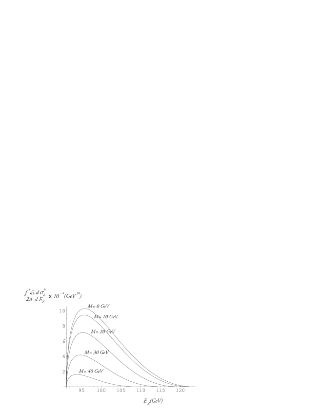
Figure 6: Differential cross section for single-Z processes as a function of the outgoing Z energy for different branon masses and for a center of mass energy $\sqrt{s}=206$ GeV. The dependence on $f$ and $n$ has been factorized out.

7.3 Bounds from single-Z processes

As in the single-photon case, the single-Z channel can be used to restrict the parameters of the theory. In this section we are going to calculate the total cross section summing over Z polarizations to estimate these bounds.

Again to implement the angular integration over the polar angle $\cos\theta$, we take into account the domain of the detector: $\cos\theta\in[-d,d]$, with $d=0.96$. The behavior of the cross section in terms of the outgoing Z energy is represented in Figure 6 for different branon masses (for $\sqrt{s}=206$ GeV). In this case, $h=g/(4\cos\theta_{W})$, $g=e/\sin\theta_{W}$, $c_{V}=-1+4\sin^{2}\theta_{W}$ and $c_{A}=1$.

The integration in the $x$ variable is done within the following limits $x\in[M_{Z}/(2\sqrt{s}),1+(M_{Z}^{2}-4M^{2})/s]$, where both the lower and the upper limits are kinematical.

To estimate a bound on the theory parameters, we will consider again the limit on the total cross section coming from new physics that can be added to the single Z channel without being detected. For LEP-II, the order of magnitude of this limit is approximately equal to that in the single photon case $\sigma_{new}\simeq 0.1$ pb.

The result for massless branons is:

$$f\geq 52n^{1/8}\mbox{GeV}.$$ (54)

and the exclusion plot can be found in Figure 5. The interior area limited by the bound curve, which is excluded, is smaller than in the single photon analysis. This is an expected result since the Z coupling to the electron field is smaller than that of the photon, and the Z mass restricts the avalaible phase space. In fact, this restricts the search only to branons with masses: $M\leq(\sqrt{s}-M_{Z})/2\simeq 57$ GeV. In the single-photon channel however, the kinematical range is larger $M\leq\sqrt{s}/2\simeq 103$ GeV. Despite this fact, the single Z channel analysis is still interesting since it provides a completely independent direct search method. In future colliders, working at very high centre-of-mass energy, the Z mass could be neglected $\sqrt{s}>>M_{Z}$, and the total cross section for the two channels will take the same form. The only difference will come from the ratio of couplings to the electron field, which is:

$$\frac{\sigma_{Z}}{\sigma_{\gamma}}(\sqrt{s}>>M_{Z})\simeq\frac{(4\sin^{2}{\theta_{W}}-1)^{2}+1}{16\cos^{2}{\theta_{W}}\sin^{2}{\theta_{W}}}\simeq 0.37,$$ (55)

where we have use the value $\sin^{2}{\theta_{W}}=0.22$. This implies that provided the rest of the analysis remains unchanged, the bounds on $f$ which come from these two processes are similar:

$$\frac{f(\sigma_{Z})}{f(\sigma_{\gamma})}(\sqrt{s}>>M_{Z})\simeq(0.37)^{1/8}\simeq 0.88,$$ (56)

Although, in general, the single-Z channel has more background compared to the single photon case, implying lower precision, however it allows us to perform analysis depending on the polarization which could improve the bounds.

Since branon effects grow strongly with energy, it is not surprising that the bounds from direct searches with ($\sqrt{s}\simeq 200$ GeV) are more constraining than the indirect ones, in which the energy scale is set by the Z mass ($M_{Z}\simeq 90$ GeV). However, because this is an effective theory the growth with energy of the cross sections will eventually violate unitarity. At that point the approximation will no longer be valid. It is also interesting to note that the present bounds improve the astrophysical ones for massless branons, coming from the 1987a supernova, from which $f>10$ GeV [10].

8 Prospects for future linear colliders

Several proposals for the construction of $e^{+}e^{-}$ linear colliders in the TeV range are currently under study. The TESLA (TeV Energy Superconducting Linear Accelerator) [17], the NLC (Next Linear Collider) [18] and the JLC (Japanese Linear Collider) [19] are examples of the first generation of these colliders, whereas the CLIC (Compact Linear Collider) [20] would correspond to the second generation. In this section we discuss the sensitivity of these colliders to a hypothetical branon signal. The study will be performed in terms of the brane tension, $f$, and the branon mass, $M$.

The physics programme of the new linear collider projects includes the measurement of electroweak parameters with improved precision, such as the invisible Z width or the $W^{\pm}$ width. However, and since the deviations due to the presence of branons increase dramatically with energy, the largest sensitivity to a branon signal is expected in direct searches like single-$\gamma$ and single-Z.

In order to estimate the sensitivity of future linear colliders to branon signals, the LEP-II study of the previous section is extended to higher center-of-mass energies. It is assumed that, at the time of construction of these accelerators, the theoretical and systematic uncertainties on Standard Model processes will be controlled at the level of the femtobarn. Under this assumption, we will estimate the sensitivity limit, $\sigma^{FLC}_{new}$, by scaling the LEP-II estimate by the expected gain in statistics:

$$\sigma^{FLC}_{new}=\sqrt{\frac{(TIL_{LEP-II})}{(TIL_{FLC})}}\,0.1~{}\mbox{pb}.$$ (57)

where $TIL_{LEP-II}\simeq 700~{}\mbox{pb}^{-1}$ is the LEP-II integrated luminosity and $0.1\,\mbox{pb}$ is the LEP-II sensitivity limit. We will consider the following values of the integrated luminosity at future colliders, $TIL_{FLC}$: $TIL_{1}\simeq 200$ fb^-1 for a first stage of TESLA, NLC or JLC, and $TIL_{2}\simeq 1000$ fb^-1 as a maximum value for a second stage. For CLIC we will assume the same total integrated luminosity: $TIL_{CLIC}=TIL_{2}\simeq 1000$ fb^-1. The cross section bounds for both luminosity choices are similar: $\sigma_{new}^{1}=6$ fb and $\sigma_{new}^{2}=\sigma^{CLIC}_{new}=3$ fb.

The critical parameter in the analysis is the center-of-mass energy, $E_{CM}$. In the single photon channel, this leads to limits on $f$ for any branon mass $M<E_{CM}/2$. In particular the limit for massless branons ($f_{0}$) increases proportionally to $E_{CM}^{3/4}$ according to Eq.(51). Assuming a center-of-mass energy for the first stage of the first generation of linear collider of approximately $500$ GeV, $1$ TeV for its second stage and $5$ TeV for CLIC, we obtain the following limits for $f_{0}$ in the case of a single branon: $f_{0\,\gamma}^{1}>398$ GeV, $f_{0\,\gamma}^{JLC}>758$ GeV and $f_{0\,\gamma}^{CLIC}>2.64$ TeV. The results of a full study in the $(f,M)$ plane and in different experimental contexts are presented in Figure 7.

For the single-Z channel, the bounds are less restrictive: $f_{0\,Z}^{1}>205$ GeV, $f_{0\,Z}^{2}>450$ GeV an $f_{0\,Z}^{CLIC}>1.87$ TeV. Obviously, the study in this case is only applicable to branon masses below $(E_{CM}-M_{Z})/2$, due to kinematic constraints. The excluded regions in the $(f,M)$ plane are also shown in Figure 7.

Figure 7: Predicted experimental accessible regions in the $f-M$ plane via single-photon and single-Z processes. Different center-of-mass energies ($E_{CM}$) and total integrated luminosities (TIL) at future $e^{+}e^{-}$ linear colliders are considered.

9 Summary and conclusions

In this work a brane-world scenario where the brane tension scale $f$ is much smaller than the fundamental gravitational scale $M_{F}$ has been considered. For this case, the relevant low-energy degrees of freedom are the brane SM particles and the brane oscillations or branons. From the corresponding effective action, and including also the effects of a possible branon non-zero mass, we have obtained the relevant Feynman rules for the couplings of branons to SM particles. They have allowed us to compute the decay rates and cross-sections for the different processes relevant for branon production in electron-positron colliders. We have used the information coming from LEP in order to get different exclusion plots on the branon mass and the tension scale plane. Single-photon production turns out to be the most efficient process in order to set bounds on the brane parameters $f$ and $M$. We have also extended the analysis to future electron-positron colliders. The corresponding exclusion plots that could be obtained in case that branons were not observed, have been also shown.

The work presented here should be complemented with a parallel analysis for electron-hadron colliders such as HERA and hadron-hadron colliders such as the Tevatron or the LHC, and with other bounds on $f$ and $M$ that could come from astrophysics and cosmology. Work is already in progress in these directions. In particular, concerning cosmology, it is interesting to notice that the allowed range of parameters suggests that branons could have weak couplings and large masses. This makes them natural dark matter candidates. In fact, an explicit calculation shows that their relic abundance can be cosmologically relevant and could account for the fraction of one third of the total energy density of the universe in the form of dark matter presently favoured by observations. These results will be presented elsewhere [21].

Acknowledgements: This work has been partially supported by the DGICYT (Spain) under the project numbers PB98-0782, AEN99-0305, FPA 2000-0956 and BFM2000-1326, and also by the director, Office of Science, Office of High Energy and Nuclear Physics of the U.S. Departament of Energy under Contract DE-AC03-76SF00098. A.D. acknowledges support from the Universidad Complutense del Amo Program.

Appendix A Branon vertices

We show the Feynman rules with leaving momenta for massive branons, including the interaction vertices between two branons and the SM particles. The dependence on the momenta of the different particles is explicitly written. We have used the notation in [6]. Different expressions in the case of massless branons have been derived in [11]. In that reference the fermionic equations of motion are imposed on the Feynman rules. In any case, as a consistency check, we have seen that our final results are the same in both cases.

A.1 $V1[p_{1},p_{2},p_{3},p_{4}]$

$\pi^{\alpha}(p_{3})$ $\pi^{\beta}(p_{4})$ $\bar{\psi}(p_{1})$ $\psi(p_{2})$	$\equiv$	$V1[p_{1},p_{2},p_{3},p_{4}]$

$$V1 = \frac{-i\delta^{\alpha\beta}}{4f^{4}}\{\gamma^{\mu}p_{4\mu}(p_{3},p_{1}-p_{2})+\gamma^{\mu}p_{3\mu}(p_{4},p_{1}-p_{2})$$ (58)

$$- \gamma^{\mu}(p_{1\mu}-p_{2\mu})(\frac{3}{2}M^{2}+2(p_{3},p_{4}))$$

$$+ 4m_{\psi}((p_{3},p_{4})+M^{2})\}.$$

A.2 $V2_{\mu\nu}^{ab}[p_{1},p_{2},p_{3},p_{4}]$

$\pi^{\alpha}(p_{3})$ $\pi^{\beta}(p_{4})$ $A^{b}_{\nu}(p_{2})$ $A^{a}_{\mu}(p_{1})$	$\equiv$	$V2_{\mu\nu}^{ab}[p_{1},p_{2},p_{3},p_{4}]$

$$V2_{\mu\nu}^{ab} = \frac{i\delta^{ab}\delta^{\alpha\beta}}{f^{4}}\{p_{1\nu}p_{3\mu}(p_{2},p_{4})+p_{3\nu}p_{2\mu}(p_{1},p_{4})$$

$$+ p_{1\nu}p_{4\mu}(p_{2},p_{3})+p_{4\nu}p_{2\mu}(p_{1},p_{3})$$

$$- \eta_{\mu\nu}((p_{1},p_{4})(p_{2},p_{3})+(p_{1},p_{3})(p_{2},p_{4})-(p_{1},p_{2})(p_{3},p_{4}))$$

$$- (p_{1},p_{2})(p_{4\nu}p_{3\mu}+p_{3\nu}p_{4\mu})-(p_{3},p_{4})(p_{1\nu}p_{2\mu})$$

$$- \frac{1}{2}M_{a}^{2}(2p_{4\nu}p_{3\mu}+2p_{3\nu}p_{4\mu}-2\eta_{\mu\nu}(p_{3},p_{4})-\eta_{\mu\nu}M^{2})\},$$

where we have used the flat background metric to contract indices in the Fadeev-Popov Lagrangian.

A.3 $V3^{a}_{\mu}[p_{3},p_{4}]$

$\pi^{\alpha}(p_{3})$ $\pi^{\beta}(p_{4})$ $\bar{\psi}(p_{1})$ $\psi(p_{2})$ $A^{a}_{\mu}(p_{5})$	$\equiv$	$V3^{a}_{\mu}[p_{3},p_{4}]$

$$V3^{a}_{\mu} = \frac{-hT^{a}\delta^{\alpha\beta}}{4f^{4}}\{2\gamma^{\nu}p_{4\nu}p_{3\mu}+2\gamma^{\nu}p_{3\nu}p_{4\mu}$$ (60)

$$+ \gamma_{\mu}(-3M^{2}-4(p_{3},p_{4})\}(c_{V}-c_{A}\gamma_{5}).$$

A.4 $V4_{\mu\nu\lambda}^{abc}[p_{1},p_{2},p_{3},p_{4},p_{5}]$

$\pi^{\alpha}(p_{3})$ $\pi^{\beta}(p_{4})$ $A^{b}_{\mu}(p_{1})$ $A^{c}_{\nu}(p_{2})$ $A^{a}_{\lambda}(p_{5})$	$\equiv$	$V4_{\mu\nu\lambda}^{abc}[p_{1},p_{2},p_{3},p_{4},p_{5}]$

$$V4_{\mu\nu\lambda}^{abc} = \frac{hC^{abc}\delta^{\alpha\beta}}{f^{4}}\{p_{1\nu}(p_{3\mu}p_{4\lambda}+p_{3\lambda}p_{4\mu})-p_{1\lambda}(p_{3\mu}p_{4\nu}+p_{3\nu}p_{4\mu})$$

$$+ p_{2\lambda}(p_{3\nu}p_{4\mu}+p_{3\mu}p_{4\nu})-p_{2\mu}(p_{3\nu}p_{4\lambda}+p_{3\lambda}p_{4\nu})$$

$$+ p_{5\mu}(p_{3\nu}p_{4\lambda}+p_{3\lambda}p_{4\nu})-p_{5\nu}(p_{3\mu}p_{4\lambda}+p_{3\lambda}p_{4\mu})$$

$$+ \eta_{\lambda\nu}((p_{3},p_{4})(p_{2\mu}-p_{5\mu})+p_{4\mu}(p_{5}-p_{2},p_{3})+p_{3\mu}(p_{5}-p_{2},p_{4}))$$

$$+ \eta_{\lambda\mu}((p_{3},p_{4})(p_{5\nu}-p_{1\nu})+p_{4\nu}(p_{1}-p_{5},p_{3})+p_{3\nu}(p_{1}-p_{5},p_{4}))$$

$$+ \eta_{\mu\nu}((p_{3},p_{4})(p_{1\lambda}-p_{2\lambda})+p_{4\lambda}(p_{2}-p_{1},p_{3})+p_{3\lambda}(p_{2}-p_{1},p_{3}))\}$$

A.5 $V5[p_{1},p_{2},p_{3},p_{4}]$

$\pi^{\alpha}(p_{3})$ $\pi^{\beta}(p_{4})$ $\phi^{\dagger}(p_{1})$ $\phi(p_{2})$	$\equiv$	$V5[p_{1},p_{2},p_{3},p_{4}]$

$$V5 = \frac{i\delta^{\alpha\beta}}{f^{4}}\left\{-[(p_{3},p_{4})+M^{2}][(p_{1},p_{2})+m_{\phi}^{2}]\right.$$ (62)

$$+ \left.(p_{1},p_{3})(p_{4},p_{2})+(p_{2},p_{3})(p_{4},p_{1})+\frac{1}{2}M^{2}(p_{1},p_{2})\right\}.$$

A.6 $V6^{a}_{\mu}[p_{3},p_{4}]$

$\pi^{\alpha}(p_{3})$ $\pi^{\beta}(p_{4})$ $\phi^{\dagger}(p_{1})$ $\phi(p_{2})$ $A^{a}_{\mu}(p_{5})$	$\equiv$	$V6^{a}_{\mu}[p_{3},p_{4}]$

$$V6^{a}_{\mu} = \frac{hT^{a}\delta^{\alpha\beta}}{f^{4}}\{(p_{1}-p_{2})_{\mu}[(p_{3},p_{4})+\frac{1}{2}M^{2}]$$ (63)

$$+ (p_{1}-p_{2},p_{3})p_{4\mu}+(p_{1}-p_{2},p_{4})p_{3\mu}\}.$$

A.7 $V7^{ab}_{\mu\nu}[p_{3},p_{4}]$

$\pi^{\alpha}(p_{3})$ $\pi^{\beta}(p_{4})$ $\phi^{\dagger}(p_{1})$ $\phi(p_{2})$ $A^{a}_{\mu}(p_{5})$ $A^{b}_{\nu}(p_{6})$	$\equiv$	$V7^{ab}_{\mu\nu}[p_{3},p_{4}]$

$$V7^{ab}_{\mu\nu} = \frac{-ih^{2}\{T^{a},T^{b}\}\delta^{\alpha\beta}}{f^{4}}\{[(p_{3},p_{4})+\frac{1}{2}M^{2}]\eta_{\mu\nu}-p_{3\mu}p_{4\nu}-p_{4\mu}p_{3\nu}\}.$$ (64)

A.8 $V8^{abcd}_{\mu\nu\rho\sigma}[p_{3},p_{4}]$

$\pi^{\alpha}(p_{3})$ $\pi^{\beta}(p_{4})$ $A^{c}_{\rho}(p_{5})$ $A^{d}_{\sigma}(p_{6})$ $A^{a}_{\mu}(p_{1})$ $A^{b}_{\nu}(p_{2})$	$\equiv$	$V8^{abcd}_{\mu\nu\rho\sigma}[p_{3},p_{4}]$

$$V8^{abcd}_{\mu\nu\rho\sigma}[p_{3},p_{4}] = \frac{ih^{2}\delta^{\alpha\beta}}{f^{4}}\{C^{eab}C^{ecd}[\eta_{\nu\sigma}(p_{3\rho}p_{4\mu}+p_{3\mu}p_{4\rho})$$ (65)

$$- \eta_{\nu\rho}(p_{3\sigma}p_{4\mu}+p_{3\mu}p_{4\sigma})$$

$$+ \eta_{\mu\sigma}(\eta_{\nu\rho}(p_{3},p_{4})-p_{3\rho}p_{4\nu}-p_{3\nu}p_{4\rho})$$

$$- \eta_{\mu\rho}(\eta_{\nu\sigma}(p_{3},p_{4})-p_{3\sigma}p_{4\nu}-p_{3\nu}p_{4\sigma})]$$

$$+ C^{eac}C^{ebd}[\eta_{\nu\mu}(p_{3\rho}p_{4\sigma}+p_{3\sigma}p_{4\rho})$$

$$- \eta_{\nu\rho}(p_{3\sigma}p_{4\mu}+p_{3\mu}p_{4\sigma})$$

$$+ \eta_{\mu\sigma}(\eta_{\nu\rho}(p_{3},p_{4})-p_{3\rho}p_{4\nu}-p_{3\nu}p_{4\rho})$$

$$- \eta_{\sigma\rho}(\eta_{\nu\mu}(p_{3},p_{4})-p_{3\mu}p_{4\nu}-p_{3\nu}p_{4\mu})]$$

$$+ C^{ead}C^{ebc}[\eta_{\nu\mu}(p_{3\rho}p_{4\sigma}+p_{3\sigma}p_{4\rho})$$

$$- \eta_{\nu\sigma}(p_{3\rho}p_{4\mu}+p_{3\mu}p_{4\rho})$$

$$+ \eta_{\mu\rho}(\eta_{\nu\sigma}(p_{3},p_{4})-p_{3\sigma}p_{4\nu}-p_{3\nu}p_{4\sigma})$$

$$- \eta_{\sigma\rho}(\eta_{\nu\mu}(p_{3},p_{4})-p_{3\mu}p_{4\nu}-p_{3\nu}p_{4\mu})]\}.$$

Appendix B Probability amplitudes

The probability amplitudes are easily calculated from the Feynman rules introduced before:

B.1 $M1$: $\bar{\psi}(p_{1}),\psi(p_{2})\longrightarrow\pi(k_{1})\pi(k_{2})A^{a}_{\mu}(q)$

There are four different diagrams that contribute to the tree-level amplitude of this process:

which is given by the following expression:

$$M1[p_{1},p_{2},k_{1},k_{2},q]=\bar{v}[p1]\{V3^{a}_{\mu}[k_{1},k_{2}]\varepsilon^{\mu,a}[q,\sigma 1]$$ (66)

$$+V11^{a}_{\mu}\varepsilon^{\mu,a}[q,\sigma 1]i\Delta_{(f)}[p_{1}-q]V1[-(p_{1}-q),-p_{2},k_{1},k_{2}]$$

$$+V1[-p_{1},-(p_{2}-q),k_{1},k_{2}]i\Delta_{(f)}[-(p_{2}-q)]V11^{a}_{\mu}\varepsilon^{\mu,a}[q,\sigma 1]$$

$$+V11^{c}_{\lambda}i\Delta^{\lambda\nu,cb}_{(A)}[(p_{1}+p_{2})]V2_{\mu\nu}^{ab}[q,-(p_{1}+p_{2}),k_{1},k_{2}]\varepsilon^{\mu,a}[q,\sigma 1]\}u[p2].$$

The fermion $(i\Delta_{(f)})$ and gauge boson $(i\Delta_{(A)})$ propagators have the usual expression in the Standard Model in renormalizable gauges, and we have used the standard vertex between gauge and fermions fields:

$A^{a}_{\mu}(p_{3})$ $\bar{\psi}(p_{1})$ $\psi(p_{2})$	$\equiv$	$V11^{a}_{\mu}\equiv h\gamma_{\mu}T^{a}(c_{V}-c_{A}\gamma_{5})$

B.2 $M2$: $A^{a}_{\mu}(q)\longrightarrow\pi(k_{1})\pi(k_{2})\bar{\psi}(p_{1}),\psi(p_{2})$

If there are massive gauge bosons in the theory, branons contribute to their decay through these processes, whose probability amplitude can be related to the previous one by:

$$M2[p_{1},p_{2},k_{1},k_{2},q]=M1[-p_{1},-p_{2},k_{1},k_{2},-q],$$ (67)

where in the right hand side, the spinors have been changed as follows $\bar{v}[p_{1}]\rightarrow\bar{u}[p_{1}]$ and $u[p_{2}]\rightarrow v[p_{2}]$.

Appendix C Integrals over two-body phase space

Integrals over the two-body phase space of branons can be easily performed using:

$$I_{\mu\nu\rho\sigma} \equiv \int d^{4}k_{1}d^{4}k_{2}\delta(k_{1}^{2}-M^{2})\delta(k_{2}^{2}-M^{2})\delta^{(4)}(k-k_{1}-k_{2})k_{1\mu}k_{1\nu}k_{2\rho}k_{2\sigma})$$

$$= C_{1}k_{\mu}k_{\nu}k_{\rho}k_{\sigma}+C_{2}k^{4}(\eta_{\mu\nu}\eta_{\rho\sigma}+\eta_{\mu\rho}\eta_{\nu\sigma}+\eta_{\mu\sigma}\eta_{\nu\rho})$$

$$+ C_{3}k^{2}(k_{\mu}k_{\nu}\eta_{\rho\sigma}+k_{\rho}k_{\sigma}\eta_{\mu\nu})$$

$$+ C_{4}k^{2}(k_{\mu}k_{\rho}\eta_{\nu\sigma}+k_{\nu}k_{\sigma}\eta_{\mu\rho}+k_{\mu}k_{\sigma}\eta_{\rho\nu}+k_{\rho}k_{\nu}\eta_{\mu\sigma})$$

$$I^{m}_{\mu\nu} \equiv \int d^{4}k_{1}d^{4}k_{2}\delta(k_{1}^{2}-M^{2})\delta(k_{2}^{2}-M^{2})\delta^{(4)}(k-k_{1}-k_{2})k_{1\mu}k_{2\nu}$$ (69)

$$= C^{m}_{1}k_{\mu}k_{\nu}+C^{m}_{2}k^{2}\eta_{\mu\nu}$$

$$I^{s}_{\mu\nu} \equiv \int d^{4}k_{1}d^{4}k_{2}\delta(k_{1}^{2}-M^{2})\delta(k_{2}^{2}-M^{2})\delta^{(4)}(k-k_{1}-k_{2})k_{1\mu}k_{1\nu}$$ (70)

$$= C^{s}_{1}k_{\mu}k_{\nu}+C^{s}_{2}k^{2}\eta_{\mu\nu}$$

And the same result by changing $k_{1}$ for $k_{2}$.

$$I^{0} \equiv \int d^{4}k_{1}d^{4}k_{2}\delta(k_{1}^{2}-M^{2})\delta(k_{2}^{2}-M^{2})\delta^{(4)}(k-k_{1}-k_{2})$$ (71)

$$= C_{0}$$

where

$$C_{0} = \frac{\pi}{2}\sqrt{1-\frac{4M^{2}}{k^{2}}}$$

$$C_{1} = \frac{\pi}{60k^{4}}\sqrt{1-\frac{4M^{2}}{k^{2}}}(k^{4}+2k^{2}M^{2}+6M^{4})$$

$$C_{1}^{m} = \frac{\pi}{12k^{2}}\sqrt{1-\frac{4M^{2}}{k^{2}}}(k^{2}+2M^{2})$$

$$C_{1}^{s} = \frac{\pi}{6k^{2}}\sqrt{1-\frac{4M^{2}}{k^{2}}}(k^{2}-M^{2})$$

$$C_{2} = \frac{\pi}{480k^{4}}\sqrt{1-\frac{4M^{2}}{k^{2}}}(k^{2}-4M^{2})^{2}$$

$$C_{2}^{m} = \frac{\pi}{24k^{2}}\sqrt{1-\frac{4M^{2}}{k^{2}}}(k^{2}-4M^{2})$$

$$C_{2}^{s} = -\frac{\pi}{24k^{2}}\sqrt{1-\frac{4M^{2}}{k^{2}}}(k^{2}-4M^{2})$$

$$C_{3} = -\frac{\pi}{240k^{4}}\sqrt{1-\frac{4M^{2}}{k^{2}}}(3k^{4}-14k^{2}M^{2}+8M^{4})$$

$$C_{4} = \frac{\pi}{120k^{4}}\sqrt{1-\frac{4M^{2}}{k^{2}}}(k^{4}-3k^{2}M^{2}-4M^{4})$$ (72)

Appendix D Polarized cross sections

In this section we give the expressions for the cross sections of the process:

$$\sigma_{A}:\bar{\psi}(p_{1}),\psi(p_{2})\longrightarrow\pi(k_{1}),\pi(k_{2}),A^{a}_{\mu}(q)$$ (73)

for the different polarizations of the outgoing gauge field. We have used the definition:

$$q^{\mu} = (q_{0},|\overrightarrow{q}|\sin\theta\cos\phi,|\overrightarrow{q}|\sin\theta\sin\phi,|\overrightarrow{q}|\cos\theta),$$ (74)

The polarization vectors read:

$$\epsilon^{\mu}_{0} = \frac{1}{M}(|\overrightarrow{q}|,q_{0}\sin\theta\cos\phi,q_{0}\sin\theta\sin\phi,q_{0}\cos\theta);$$ (75)

$$\epsilon^{\mu}_{\pm} = \frac{1}{\sqrt{2}}(0,-\cos\theta\cos\phi\pm i\sin\phi,-\cos\theta\sin\phi\mp i\cos\phi,\sin\theta).$$

For the longitudinal polarization ($\epsilon^{\mu}_{0}$), we get:

$$\frac{d\sigma_{A}}{dxd\cos\theta} = \frac{|h|^{2}}{4\pi}\frac{(c_{V}^{2}+c_{A}^{2})M_{a}^{2}n}{122880f^{8}\pi^{2}(s-M_{a}^{2})^{2}}\sqrt{1-\frac{4M^{2}}{s(1-x)+M_{a}^{2}}}$$ (76)

$$\sqrt{s(sx^{2}-4M_{a}^{2})}\{5M^{2}(2(s(1-x)+M_{a}^{2})-5M^{2})\{sx^{2}\sin^{2}\theta\}$$

$$+ \frac{(s(1-x)+M_{a}^{2}-4M^{2})^{2}}{(4M_{a}^{2}(M_{a}^{2}+s(1-x))+s(sx^{2}-4M_{a}^{2})\sin^{2}\theta)^{2}}$$

$$\{32(s(1-x)+M_{a}^{2})^{3}(M_{a}^{2}+s)^{2}-16(s(1-x)+M_{a}^{2})^{2}$$

$$[M_{a}^{6}+2M_{a}^{4}sx(1-x)+M_{a}^{2}s^{2}(9-2x^{2})$$

$$+ 2s^{3}(1-x-x^{2})]\sin^{2}\theta-4s[4M_{a}^{8}+M_{a}^{6}s(12-20x+15x^{2})$$

$$- M_{a}^{4}s^{2}(4+8x-37x^{2}+11x^{3}+4x^{4})$$

$$+ M_{a}^{2}s^{3}(-12+28x-7x^{2}-6x^{3}-10x^{4}+4x^{5})$$

$$+ s^{4}x^{2}(3-7x+2x^{2}+2x^{3})]\sin^{4}\theta$$

$$+ 2s^{3}(2+x^{2})(sx^{2}-4M_{a}^{2})^{2}\sin^{6}\theta\}\}.$$

The contributions of the transverse polarizations ($\epsilon_{\mu}^{+}$ or $\epsilon_{\mu}^{-}$) are the same and they are given by:

$$\frac{d\sigma_{A}}{dxd\cos\theta} = \frac{|h|^{2}}{4\pi}\frac{(c_{V}^{2}+c_{A}^{2})n}{122880f^{8}\pi^{2}(s-M_{a}^{2})^{2}}\sqrt{1-\frac{4M^{2}}{s(1-x)+M_{a}^{2}}}$$ (77)

$$\sqrt{s(sx^{2}-4M_{a}^{2})}\{10M^{2}M_{a}^{4}(2(s(1-x)+M_{a}^{2})-5M^{2})\{2-\sin^{2}\theta\}$$

$$+ \frac{(s(1-x)+M_{a}^{2}-4M^{2})^{2}}{(4M_{a}^{2}(M_{a}^{2}+s(1-x))+s(sx^{2}-4M_{a}^{2})\sin^{2}\theta)^{2}}$$

$$\{16M_{a}^{4}(s(1-x)+M_{a}^{2})^{2}[9M_{a}^{4}+M_{a}^{2}s(6-4x)+s^{2}(5-4x+2x^{2})]$$

$$+ 2[-36M_{a}^{12}+2M_{a}^{10}s(-108+40x+x^{2})$$

$$- 4M_{a}^{8}s^{2}(68-72x+6x^{2}+x^{3})$$

$$+ M_{a}^{6}s^{3}(-136+200x-54x^{2}-26x^{3}+3x^{4})$$

$$- M_{a}^{4}s^{4}(44-80x+34x^{2}+12x^{3}-13x^{4}+x^{5})$$

$$+ M_{a}^{2}s^{5}x(-8+28x-34x^{2}+21x^{3}-6x^{4})$$

$$- s^{6}x^{2}(-2+4x-3x^{2}+x^{3})]\sin^{2}\theta+s[120M_{a}^{10}$$

$$- 2M_{a}^{8}s(-148+76x+13x^{2})-M_{a}^{6}s^{2}(-8+48x+62x^{2}$$

$$- 34x^{3}+x^{4})+M_{a}^{4}s^{3}(24+8x+10x^{2}+4x^{3}-3x^{4}+x^{5})$$

$$+ M_{a}^{2}s^{4}x^{2}(-18+10x-11x^{2}+2x^{3})+s^{5}x^{4}(3(1-x)$$

$$+2x^{2})]\sin^{4}\theta-s^{2}(sx^{2}-4M_{a}^{2})^{2}[4M_{a}^{4}-2M_{a}^{2}s+s^{2}x^{2}]\sin^{6}\theta\}\}$$

References

-
[1]
N. Arkani-Hamed, S. Dimopoulos and G. Dvali,
Phys. Lett. B429, 263 (1998)
N. Arkani-Hamed, S. Dimopoulos and G. Dvali, Phys. Rev. D59, 086004 (1999)
I. Antoniadis, N. Arkani-Hamed, S. Dimopoulos and G. Dvali, Phys. Lett. B436 257 (1998) -
[2]
A. Perez-Lorenzana, AIP Conf.Proc. 562
53 (2001)
V.A. Rubakov, Phys.Usp. 44 (2001) 871, Usp.Fiz.Nauk 171, 913 (2001)
Y. A. Kubyshin hep-ph/0111027 - [3] J. Hewett and M. Spiropulu, Ann. Rev. Nucl. Part. Sci. 52, 397-424 (2002).
- [4] M. Bando, T. Kugo, T. Noguchi and K. Yoshioka, Phys. Rev. Lett. 83, 3601 (1999)
- [5] R. Sundrum, Phys. Rev. D59, 085009 (1999)
- [6] A. Dobado and A.L. Maroto Nucl. Phys. B592, 203 (2001)
-
[7]
H. Murayama and J. D. Wells Phys.Rev. D65
056011 (2002)
S. C. Park and H. S. Song, hep-ph/0109258 - [8] R. Contino, L. Pilo, R. Rattazzi and A. Strumia JHEP 0106,005 (2001)
- [9] Q. S. Yan and D.S. Du Phys.Rev., D65 094034(2002)
- [10] T. Kugo and K. Yoshioka, Nucl. Phys. B594, 301(2001)
- [11] P. Creminelli and A. Strumia, Nucl. Phys. B596 125 (2001)
- [12] J.A.R. Cembranos, A. Dobado and A.L. Maroto, Phys.Rev. D65:026005, (2002)
- [13] A Combination of Preliminary Electroweak Measurements and Constraints on the Standard Model. The LEP Collaborations, the LEP Electroweak Working Group and the SLD Heavy Flavour Group, LEPEWWG/2002-01, hep-ex/0112021.
- [14] E. Torrence, Proceedings of the Conference of Physics in Collisions, Seoul, South Korea, 28-30 June 2001, hep-ex/0110003.
- [15] L3 Collab., P. Achard et al., Phys. Lett. B531, 28-38 (2002).
- [16] Search for the Standard Model Higgs Boson at LEP. The ALEPH, DELPHI, L3 and OPAL Collaborations, and the LEP Working Group for Higgs Boson Searches, http://cern.ch/LEPHIGGS/www/, LHWG Note/2001-03, hep-ex/0107029.
- [17] The TESLA-N Collab., the ECFA/DESY LC Physics Working Group et al., TESLA Technical Design Report, DESY 2001-011, ECFA 2001-23 (2001).
- [18] The NLC Collab., 2001 Report on the Next Linear Collider, SLAC-R-571, FERMILAB-Conf-01-075-E, LBNL-PUB-47935, UCRL-ID-144077 (2001).
- [19] N. Akasaka et al., JLC Design Study, KEK-REPORT-97-1 (1997).
- [20] A 3 TeV Linear Colider Based on CLIC Technology, The CLIC Study Team, G. Guignard (editor), CERN-2000-008 (2000).
- [21] J.A.R. Cembranos, A. Dobado and A.L. Maroto, hep-ph/0302041.