LMA MSW solution of the solar neutrino problem and first KamLAND results

P. C. de Holanda¹ and A. Yu. Smirnov^2,3

(1) Instituto de Física Gleb Wataghin - UNICAMP, 13083-970 Campinas SP, Brasil
(2) The Abdus Salam International Centre for Theoretical Physics, I-34100 Trieste, Italy
(3) Institute for Nuclear Research of Russian Academy of Sciences, Moscow 117312, Russia

The first KamLAND results are in a very good agreement with the predictions made on the basis of the solar neutrino data and the LMA realization of the MSW mechanism. We perform a combined analysis of the KamLAND (rate, spectrum) and the solar neutrino data with a free boron neutrino flux $f_{B}$. The best fit values of neutrino parameters are $\Delta m^{2}=7.3\cdot 10^{-5}$ eV², $\tan^{2}\theta=0.41$ and $f_{B}=1.05$ with the $1\sigma$ intervals: $\Delta m^{2}=(6.2-8.4)\cdot 10^{-5}$ eV², $\tan^{2}\theta=0.33-0.54$. We find the $3\sigma$ upper bounds: $\Delta m^{2}<2.8\cdot 10^{-4}$ eV² and $\tan^{2}\theta<0.84$, and the lower bound $\Delta m^{2}>4\cdot 10^{-5}$ eV². At 99% C.L. the KamLAND spectral result splits the LMA region into two parts with the preferred one at $\Delta m^{2}<10^{-4}$ eV². The higher $\Delta m^{2}$ region is accepted at about $2\sigma$ level. We show that effects of non-zero 13-mixing, $\sin^{2}\theta_{13}\leq 0.04$, are small leading to a slight improvement of the fit in higher $\Delta m^{2}$ region. In the best fit point we predict for SNO: CC/NC $=0.33^{+0.05}_{-0.03}$ and $A_{DN}^{SNO}=2.8\pm 0.8\%$ (68% C.L.), and $A_{DN}^{SNO}<9\%$ at the $3\sigma$ level. Further improvements in the determination of the oscillation parameters are discussed and implications of the solar neutrino and KamLAND results are considered.

1 Introduction

The first KamLAND results [1] are the last (or almost last) step in resolution of the long-standing solar neutrino problem [2]. “In the context of two flavor neutrino oscillations with the CPT invariance, the KamLAND results exclude all oscillation solutions of this problem but the ‘Large mixing angle’ solution” [1]. In fact, KamLAND excludes also all non-oscillation solutions based on neutrino spin-flip in the magnetic fields of the Sun, on the non-standard neutrino interactions, etc.. More precisely, KamLAND excludes them as the dominant mechanisms of the solar neutrino conversion.

Soon after the suggestion of the MSW mechanism [3], the “MSW triangle” [4] had been constructed in the $\Delta m^{2}-\sin^{2}2\theta$ plane which corresponds to 1/4 - 1/3 suppression of the Argon production rate [5]. The region around the upper right corner of this triangle, or large $\sin^{2}2\theta$ part of its horizontal side (“the adiabatic solution”) is what we call now the LMA region.

Kamiokande [6], SAGE [7] and GALLEX [8] have disintegrated the triangle into pieces excluding some parts of oscillation parameter space. First, the results from Kamiokande (the absence of a strong spectrum distortion as well as the absence of strong Day-Night effect) have chipped off the LMA region. Then Gallium experiments SAGE and GALLEX, confirming LMA, have splitted the diagonal side of the triangle into SMA and LOW. Apart from that vacuum oscillation solutions (VO) were always present.

For a long time SMA was the favored solution and LMA was considered as an non excluded possibility. Things changed in 1998 when Super-Kamiokande [9] has testified against SMA (the flatness of spectrum and the absence of a peak in the zenith angle distribution of events in the Earth core bin). Soon after that, the analysis of the Super-Kamiokande data for 708 days of operation allowed us [10] to conclude that solar neutrino results provide hints that the LMA solution could be correct (see also analysis in [11]). Since that time LMA continuously reinforced its position.

Super-Kamiokande [9] and then SNO [12] have accomplished genesis of the triangle. They have practically excluded SMA, disfavored LOW and VO, and shifted the LMA region to larger $\Delta m^{2}$ (small Day-Night asymmetry at Super-Kamiokande) and smaller mixings (small ratio of CC/NC events at SNO).

By the time of the KamLAND announcement, the solar neutrino data [5, 7, 8, 9, 12, 13, 14] have definitely selected LMA as the most favorable solution based on neutrino mass and mixing [15, 16]. The best fit point from the free boron neutrino flux fit [16] is

$$\Delta m^{2}=6.15\cdot 10^{-5}{\rm eV}^{2},~{}~{}~{}\tan^{2}\theta=0.41,~{}~{}~{}f_{B}=1.05,$$ (1)

where $f_{B}\equiv F_{B}/F_{B}^{SSM}$ is the boron neutrino flux in the units of the Standard Solar Model predicted flux [17].

On basis of the solar neutrino results (and the assumption of the CPT invariance) predictions for the KamLAND experiment have been calculated. A significant suppression of the signal was expected in the case of the LMA solution. The predicted ratio of the numbers of events with the visible (prompt) energies, $E_{p}$, above 2.6 MeV with and without oscillations equals [16]:

$$R_{KL}^{LMA}=0.65^{+0.09}_{-0.40}~{}~{}~{}(3\sigma).$$ (2)

For other solutions of the solar neutrino problem one expected $R_{KL}=0.9-1$, where the deviation from 1 can be due to the effect of nonzero 1-3 mixing.

In the best fit point (1) the predicted spectrum has (i) a peak at $E_{p}\approx(3.0-3.6)$ MeV, (ii) a suppression of the number of events near the threshold energy $E_{p}\approx 2.6$ MeV and (iii) a significant suppression of the signal (with respect to the no-oscillation case) at the high energies: $E_{p}>(4-5)$ MeV [16]. No distortion of the spectrum is expected for the other solutions.

The first KamLAND results: both the total number of events and spectrum shape [1], are in a very good agreement with predictions:

$$R_{KL}^{exp}=0.611\pm 0.094~{}.$$ (3)

The spectral data (although not yet precise) reproduce well the features described above. As a result, the allowed “island” in the $\Delta m^{2}-\sin^{2}2\theta$ plane with the best fit KamLAND point covers the best fit point from the solar neutrino analysis [1].

In this paper we present our analysis of the KamLAND data as well as combined analysis of the solar neutrinos and KamLAND results. The impact of KamLAND on the LMA MSW solution is studied. We consider implications of the combined (solar neutrinos + KamLAND) analysis and make predictions for the future measurements.

During preparation of this paper, several studies of the first KamLAND results and solar neutrino data have been published [18] - [25]. Our conclusions are in a good agreement with results of those papers, although there are some differences. Detailed comparison of results will be done later.

2 KamLAND

In a given energy bin $a$ $(a=1,....13)$ the signal at KamLAND is determined by

$$N_{a}=A\sum_{i}\int_{E_{a}}^{E_{a}+\Delta E}dE_{p}\int dE_{p}^{\prime}P_{i}F_{i}\sigma f(E_{p},E_{p}^{\prime})~{},$$ (4)

where $\Delta E=0.425$ MeV,

$$P_{i}=\left(1-\sin^{2}2\theta_{12}\sin^{2}\frac{\Delta m^{2}_{12}L_{i}}{4E}\right)$$ (5)

is the vacuum oscillation survival probability for $i$ reactor situated at the distance $L_{i}$ from KamLAND, $F_{i}$ is the flux from $i$ reactor, $\sigma$ is the cross-section of $\bar{\nu}p\rightarrow e^{+}n$ reaction, $E_{p}$ is the observed prompt energy, $E_{p}^{\prime}$ is the true prompt energy, $f(E_{p},E_{p}^{\prime})$ is the energy resolution function, $A$ is the factor which takes into account the fiducial volume, the time of observation, etc.. We sum over all reactors contributing appreciable to the flux at KamLAND.

The suppression factor of the total number of (reactor neutrino) events above certain threshold is defined as:

$$R_{KL}(\Delta m^{2},\tan^{2}\theta)\equiv\frac{N(\Delta m^{2},\tan^{2}\theta)}{N_{0}}~{},$$ (6)

where $N=\sum_{a}N_{a}$, $N_{a}$ is given in (4) and $N_{0}$ is the total number of events in the absence of oscillations (following KamLAND we will call $N$ and $N_{0}$ the rates).

1). KamLAND spectrum. High threshold. We perform $\chi^{2}$ analysis of the KamLAND spectrum, defining

$$\chi^{2}_{spec}=\sum_{a=1...13}\sum_{b=1...13}(N_{a}-N_{a}^{th})\sigma^{-2}_{ab}(N_{b}-N_{b}^{th})~{},$$ (7)

where $\sigma_{ab}$ is the covariance matrix in which the systematic uncertainties were propagated to the spectral bins.

We find that for $E_{p}\geq 2.6$ MeV the minimum of $\chi^{2}_{spec}$ is achieved for

$$\Delta m^{2}=7.34\cdot 10^{-5}{\rm eV}^{2},~{}~{}~{}\tan^{2}\theta=0.453,$$ (8)

and in this point $\chi^{2}/d.o.f.=2.92/11$. Notice that in contrast with the KamLAND result [1] our best fit mixing deviates from the maximal mixing.

We present in fig. 1 the contours of constant confidence level with respect to the best fit point (8) in the $(\Delta m^{2}-\tan^{2}\theta)$ plane using relation: $\chi^{2}=\chi^{2}_{min}+\Delta\chi^{2}$, where $\Delta\chi^{2}=1,3.84$ and $6.63$ for $1\sigma$, $95\%$ and $99\%$ C.L. correspondingly.

The contours manifest an oscillatory pattern in $\Delta m^{2}$ in spite of a strong averaging effect which originates from large spread in distances from different reactors. The pattern can be described in terms of oscillations with certain effective distance, $L_{eff}$, and effective oscillation phase $\phi_{eff}$:

$$\phi_{eff}=\frac{\Delta m^{2}_{12}L_{eff}}{4E},~{}~{}~{}L_{eff}\approx 165~{}{\rm km}.$$ (9)

$L_{eff}$ corresponds to the distance between KamLAND and the closest set of reactors which provides the large fraction of the antineutrino flux. Notice that $L_{eff}$ is smaller than the average (weighted with power) distance 189 km.

Let us consider the 95% allowed regions.

(i) The lowest “island” allowed by KamLAND with $\Delta m^{2}<2\cdot 10^{-5}$ eV² corresponds to the oscillation phase $\phi_{eff}<\pi/2$. This region is excluded by the absence of significant day-night asymmetry of the Super-Kamiokande signal. In this domain, the predicted asymmetry at SNO, $A_{DN}^{SNO}>17\%$, is still consistent with data.

(ii) The second allowed region, $\Delta m^{2}=(5-10)\cdot 10^{-5}$ eV², corresponds to the first oscillation maximum, $\phi_{eff}\sim\pi$ (maximum of the survival probability). It contains the best fit point.

(iii) The third island is at $\Delta m^{2}=(13-23)\cdot 10^{-5}$ eV²: it corresponds to the oscillation maximum (second maximum of the survival probability) with $\phi_{eff}\sim 2\pi$.

There is a continuum of the allowed regions above $\Delta m^{2}\sim 3\cdot 10^{-4}$ eV². The third region merges with the continuum at 99% CL.

At the $1\sigma$ level the second island is the only allowed region.

2) KamLAND rate. In fig.1 we show the regions excluded by the KamLAND rate at $95\%$ C.L.. The borders of these regions coincide with contours of constant $R_{KL}^{max}=0.80$ and $R_{KL}^{min}=0.42$ obtained in [16]). The exclusion region at $\Delta m^{2}\sim(2-5)\cdot 10^{-5}$ eV² corresponds to the first oscillation minimum (minimum of the survival probability) at KamLAND ($\phi_{eff}\sim\pi/2$). Here the suppression of the signal is too strong. Another region of significant suppression (second oscillation minimum with $\phi_{eff}=3\pi/2$) is at $\Delta m^{2}\sim(9-12)\cdot 10^{-5}$ eV².

3). KamLAND spectrum. Low threshold. We analyze the spectrum with the threshold $E_{p}^{th}=0.9$ MeV, using the same prescription for the contribution of the geological neutrinos as in [1]. The best fit point shifts with respect to (8) to larger mixing and smaller mass squared difference:

$$\Delta m^{2}=6.86\cdot 10^{-5}{\rm eV}^{2},~{}~{}~{}\tan^{2}\theta=0.48\,.$$ (10)

In fig. 2 we show the allowed regions at 68 %, 95% and 99% confidence levels.

With lowering the threshold the sensitivity to the spectrum shape increases: the measurements become sensitive not only to the dominant oscillation peak but also to the lower energy oscillation maximum. As a result, the analysis leads to stronger exclusion of the oscillation parameter space. In particular, maximal and large mixing parts become less favored than in the case of high threshold.

4). KamLAND spectrum and rate. Following procedure in [1] we have performed also combined analysis of spectrum and rate introducing the free normalization parameter of the spectrum, $R_{KL}$, and defining the $\chi^{2}$ as

$$\chi^{2}_{spec,R}=\chi^{2}_{spec}+\chi^{2}_{R},$$ (11)

where

$$\chi^{2}_{R}=\left(\frac{R_{KL}-0.611}{0.094}\right)^{2}.$$ (12)

We find results which are very close to those from our spectrum analysis. In particular, the best fit value of mixing is $\tan^{2}\theta=0.48$ and $\Delta m^{2}=7.31\cdot 10^{-5}$ eV².

As it follows from our consideration here, the values of oscillation parameters extracted from the KamLAND data, $(\Delta m^{2},~{}~{}\tan^{2}\theta)_{KL}$, are in a very good agreement with the values from independent solar neutrino analysis $(\Delta m^{2},~{}~{}\tan^{2}\theta)_{sun}$, For the best fit points (1), (8) (10) we conclude that within $1\sigma$ (see fig. 1 and fig. 2)

$$(\Delta m^{2},~{}~{}\tan^{2}\theta)_{KL}=(\Delta m^{2},~{}~{}\tan^{2}\theta)_{sun}.$$ (13)

At the same time, the data do not exclude that the solar and KamLAND parameters are different, and moreover, the difference still can be large. For instance, $(\Delta m^{2},~{}~{}\tan^{2}\theta)_{KL}$ can coincide with the present best fit point or be in the high $\Delta m^{2}$ island, whereas $(\Delta m^{2},~{}~{}\tan^{2}\theta)_{sun}$ can be at lower $\Delta m^{2}$.

3 Solar Neutrinos

We use the same data set and the same procedure of analysis as in our previous publication [16]. Here the main ingredients of the analysis are summarized.

The data sample consists of

- 3 total rates: (i) the $Ar$-production rate, $Q_{Ar}$, from Homestake [5], (ii) the $Ge-$production rate, $Q_{Ge}$ from SAGE [7] and (iii) the combined $Ge-$production rate from GALLEX and GNO [8];

- 44 data points from the zenith-spectra measured by Super-Kamiokande during 1496 days of operation [9];

- 38 day-night spectral points from SNO [13, 14].

Altogether the solar neutrino experiments provide us with 81 data points.

All the solar neutrino fluxes, but the boron neutrino flux, are taken according to SSM BP2000 [17]. The boron neutrino flux is treated as a free parameter. For the $hep-$neutrino flux we take fixed value $F_{hep}=9.3\times 10^{3}$ cm^-2 s^-1 [17, 26] .

Thus, in our analysis of the solar neutrino data as well as in the combined analysis of the solar and KamLAND results we have three fit parameters: $\Delta m^{2}$, $\tan^{2}\theta$ and $f_{B}$.

We define the contribution of the solar neutrino data to $\chi^{2}$ as

$$\chi^{2}_{sun}=\chi^{2}_{rate}+\chi^{2}_{SK}+\chi^{2}_{SNO},$$ (14)

where $\chi^{2}_{rate}$, $\chi^{2}_{SK}$ and $\chi^{2}_{SNO}$ are the contributions from the total rates, the Super-Kamiokande zenith spectra and the SNO day and night spectra correspondingly. The main result of analysis performed in [16] is given here in Eq. (1).

4 Solar neutrinos and KamLAND

We have performed two different combined fits of the data from the solar neutrino experiments and KamLAND.

1) KamLAND rate and solar neutrino data. There are 81 (solar) + 1 (KamLAND) data points - 3 free parameters = 79 d.o.f.. We define the global $\chi^{2}$ for this case as

$$\chi^{2}_{sun,R}=\chi^{2}_{sun}+\chi^{2}_{R},$$ (15)

where $\chi^{2}_{sun}$ and $\chi^{2}_{R}$ are given in (14) and (12). The minimum $\chi^{2}_{sun,R}(min)/d.o.f.=65.2/79$ corresponds to the C.L. = 86.7% . It appears at

$$\Delta m^{2}=6.03\cdot 10^{-5}{\rm eV}^{2},~{}~{}~{}\tan^{2}\theta=0.411,~{}~{}~{}f_{B}=1.05.$$ (16)

This point practically coincides with what we have obtained from the solar neutrino analysis only.

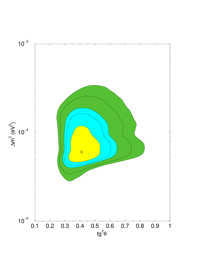
Figure 3: The allowed regions in $\tan^{2}\theta-\Delta m^{2}$ plane from a combined analysis of the solar neutrino data and the KamLAND rate, at 1$\sigma$, 90%, 95%, 99% and 3$\sigma$ C.L.. The best fit point is marked by star.

We construct the contours of constant confidence level in the $(\Delta m^{2}-\tan^{2}\theta)$ plot using the following procedure. We perform minimization of $\chi^{2}_{sun,R}$ with respect to $f_{B}$ for each point of the oscillation plane, thus getting $\chi^{2}_{sun,R}(\Delta m^{2},\tan^{2}\theta)$. Then the contours are defined by the condition $\chi^{2}_{sun,R}(\Delta m^{2},\tan^{2}\theta)=\chi^{2}_{sun,R}(min)+\Delta\chi^{2}$, where $\Delta\chi^{2}=2.3,\,4.61,\,5.99,\,9.21$ and $11.83$ are taken for $1\sigma,\,90\%,\,95\%$ and $99\%$ C.L. and $3\sigma$. The results are shown in fig. 3.

According to the figure, the main impact of the KamLAND rate is strengthening of bound on the allowed region from below due to strong suppression of the KamLAND rate at $\Delta m^{2}=(2-5)\cdot 10^{-5}$ eV² (see fig. 1) - region of the first oscillation minimum in KamLAND. The lines of constant confidence level are shifted to larger $\Delta m^{2}$. The KamLAND rate leads to a distortion (shift to smaller mixings) of contours at $\Delta m^{2}\sim 10^{-4}$ eV² where the second oscillation minimum at KamLAND is situated. The upper part of the allowed region is modified rather weakly.

2). KamLAND spectrum and solar neutrino data. We calculate

$$\chi^{2}_{global}=\chi^{2}_{sun}+\chi^{2}_{spec}~{},$$ (17)

where $\chi^{2}_{spec}$ has been defined in (7). In this case we have 81 (solar) + 13 (KamLAND) data points - 3 free parameters = 91 d.o.f.. The absolute minimum, $\chi^{2}_{global}(min)=68.2$ (which corresponds to a very high confidence level: $96.3\%$), is at

$$\Delta m^{2}=7.32\cdot 10^{-5}{\rm eV}^{2},~{}~{}~{}\tan^{2}\theta=0.409,~{}~{}~{}f_{B}=1.05.$$ (18)

The best fit value of $\Delta m^{2}$ is slightly higher than that from the solar data analysis. The solar neutrino data have higher sensitivity to mixing, whereas the KamLAND is more sensitive to $\Delta m^{2}$, as a result, in (18) the value of $\Delta m^{2}$ is close to the one determined from the KamLAND data only (8), whereas $\tan^{2}\theta$ coincides with mixing determined from the solar neutrino results (1).

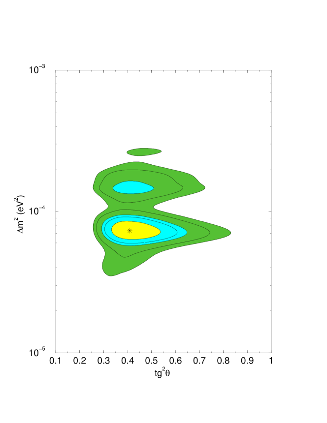
Figure 4: The allowed regions in $\tan^{2}\theta-\Delta m^{2}$ plane, from a combined analysis of the solar neutrino data and the KamLAND spectrum at 1$\sigma$, 90%, 95%, 99% and 3$\sigma$ C.L.. The best fit point is marked by star.

We construct the contours of constant confidence levels in the oscillation plane, similarly to what we did for the fit of the solar data and the KamLAND rate (fig. 4).

As compared with the solar data analysis, KamLAND practically has not changed the upper bound on mixing, but strengthened the bound on $\Delta m^{2}$. At the $3\sigma$ level we get:

$$\Delta m^{2}<2.8\cdot 10^{-4}{\rm eV}^{2},~{}~{}~{}\tan^{2}\theta<0.84,~{}~{}~{}99.73\%~{}{\rm C.L.}~{}.$$ (19)

The spectral data disintegrate the LMA region. At the $3\sigma$ level only a small spot is left in the range $\Delta m^{2}>2.5\cdot 10^{-4}$ eV².

At the 99% C.L. the rest of the region splits into two “islands” which we will refer to as the lower (l-) and higher (h-) LMA regions. (Existence of these two islands can be seen already from an overlap of the solar and KamLAND allowed regions in [1]). The l-region is characterized by

$$\Delta m^{2}=(4.7-10)\cdot 10^{-5}{\rm eV}^{2},~{}~{}~{}\tan^{2}\theta=0.27-0.75.$$ (20)

It contains the best fit point (18). The h-region is determined by

$$\Delta m^{2}=(12-20)\cdot 10^{-5}{\rm eV}^{2},~{}~{}~{}\tan^{2}\theta=0.29-0.63,$$ (21)

with best fit point at

$$\Delta m^{2}=14.5\cdot 10^{-5}{\rm eV}^{2},~{}~{}~{}\tan^{2}\theta=0.41.$$ (22)

This point is accepted with respect to the global minimum (18) at about $2\sigma$ level.

The excluded region between two islands corresponds to the second oscillation minimum ($\phi_{eff}\sim 3\pi/2$) at $E_{p}\sim(3-4)MeV$ which contradicts the spectral data.

Features of spectrum distortion. In the fig. 5 we show the prompt energy spectra of events for the best fit points in the l- and h-regions, $N_{l}(E_{p})$ and $N_{h}(E_{p})$. The spectra can be well understood in terms of the effective oscillation phase $\phi_{eff}$:

$$N(E_{p})\sim N_{0}(E_{p})\left[1+D(E_{p})\sin^{2}\phi_{eff}\right],$$ (23)

where $D(E_{p})$ is the averaging factor.

In the best fit point of l-region (18), the peak at $E_{p}\approx 3.6$ MeV corresponds to the oscillation maximum $\phi_{eff}=\pi$ (exact position of maximum of the survival probability is at $E_{p}=4.3{\rm MeV}$). The closest oscillation minimum (phase $\phi_{eff}=3\pi/2$) is at $E_{p}\approx 2.4$ MeV and the next maximum ($\phi_{eff}=2\pi$) is at $E_{p}\approx 1.8$ MeV. Due to strong averaging effect the structures below (in $E_{p}$) the main maximum are not profound and look more like a shoulder below the peak. The first oscillation minimum is at $E_{p}=7.2$ MeV.

In the case of h-region (22) the spectrum has similar structure but (due to larger $\Delta m^{2}$) the energy intervals between maxima and minima decrease. The main peak at $E_{p}\approx 3.4$ MeV corresponds now to the second oscillation maximum with $\phi_{eff}=2\pi$. One can calculate then that the next minimum ( $\phi_{eff}=5\pi/2$) is at $E_{p}\approx 2.7$ MeV and the next maximum ($\phi_{eff}=3\pi$) is at $E=2.2$ MeV. The higher energy oscillation minimum ($\phi_{eff}=3\pi/2$) is at $E=5$ MeV. This pattern can be seen in the fig. 5 which confirms validity of the effective phase consideration.

The measured spectrum, indeed, gives a hint of existence of the low energy shoulder. Evidently with the present data it is impossible to disentangle the l- and h- spectra. Substantial decrease of errors is needed. Also decrease of the energy threshold will help. According to fig. 5, $N_{l}(E_{p})>N_{h}(E_{p})$ at $E_{p}>3.5$ MeV, and $N_{l}(E_{p})<N_{h}(E_{p})$ at lower energies, especially in the interval $E_{p}=(2.0-2.5)$ MeV. Therefore for the low threshold the difference between $N_{l}(E_{p})$ and $N_{h}(E_{p})$ can not be eliminated by normalization (mixing angle). See similar discussion in [19].

Pull-off diagrams. To check the quality of the fit we have constructed the pull-off diagrams [32] which show deviations, $D_{K}$, of the predicted values of the observables $K_{bf}$ from the central experimental values, $K_{exp}$, in the units of the $1\sigma$ experimental errors, $\sigma_{K}$,:

$$D_{K}\equiv\frac{K_{bf}-K_{exp}}{\sigma_{K}},$$ (24)

where $K=Q_{Ar},~{}Q_{Ge},~{}CC/NC,~{}A_{DN}^{SNO},~{}A_{DN}^{SK},~{}R_{KL},~{}f_{B}$.

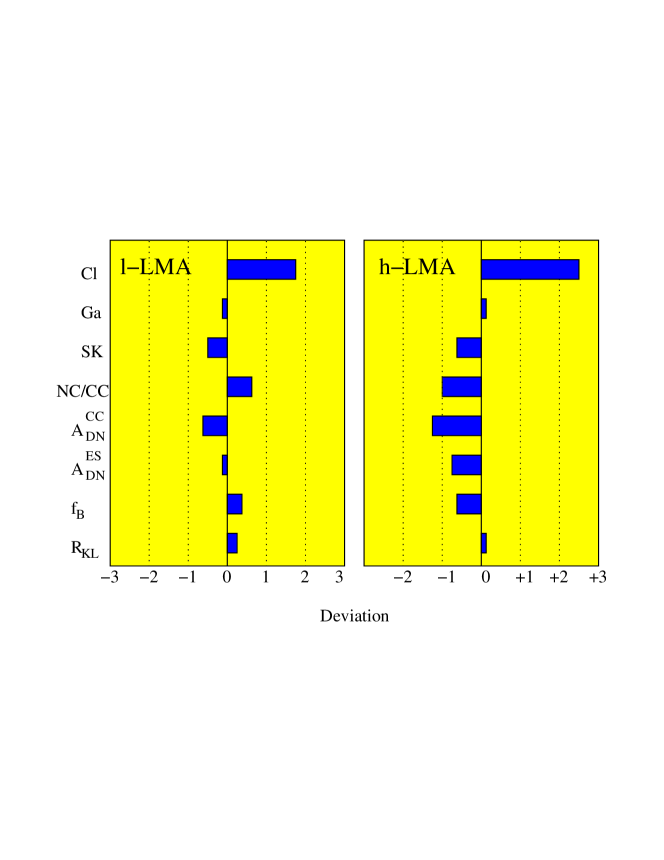
Figure 6: The pull-off diagrams for the best fit points in the l- and h- regions. Shown are deviations of the predicted values of different observables from the central experimental values in the units of $1\sigma$ (experimental).

In fig. 6 we show the pull-off diagrams for the best fit points from the l- and h-regions. In both regions the largest deviation is for the $Ar$-production rate. In the h-region: $Q_{Ar}>3.1$ SNU, which is $2.5\sigma$ above the Homestake result. In the l-region the $Q_{Ar}$ deviation is smaller: about $1.8\sigma$.

Other deviations are about $1\sigma$ or smaller; they are even smaller in the l-region. In the h-region a very small D-N asymmetry is expected. The l- and h-regions lead to the opposite sign deviations for the CC/NC ratio at SNO, and therefore future precise measurements of this ratio will discriminate among l- and h- solutions. Notice also that in h-region $f_{B}<1$.

5 Effect of 1-3 mixing

We assume that $\Delta m^{2}_{13}=\Delta m^{2}_{atm}=(2-3)\cdot 10^{-3}$ eV², and there is a non-zero admixture of $\nu_{e}$ in the third mass eigenstate described by the angle $\theta_{13}$. Both for KamLAND and for solar neutrinos the oscillations driven by $\Delta m^{2}_{13}$ are averaged out and signals are determined by the survival probabilities

$$P_{ee}=(1-\sin^{2}\theta_{13})^{2}{P}_{2}+\sin^{4}\theta_{13}\approx(1-2\sin^{2}\theta_{13}){P}_{2}.$$ (25)

Here $P_{2}=P_{2}(\Delta m^{2}_{12},\theta_{12})$ is the two neutrino vacuum oscillation probability for KamLAND and it is the two neutrino conversion probability for solar neutrinos. The factor $(1-\sin^{2}\theta_{13})^{2}$ leads to additional suppression of the KamLAND signal and shift of the allowed regions to smaller $\theta_{12}$ (see detailed study in [27]). The effect of $\theta_{13}$ on the solar neutrino analysis has been discussed in [16].

We have performed the combined analysis of the solar neutrino and KamLAND data for a fixed value of $\sin^{2}\theta_{13}$ taken at the upper bound given by the CHOOZ experiment [28]: $\sin^{2}\theta_{13}=0.04$. The number of degrees of freedom is the same as in the $2\nu$ fit and we follow procedure described in sect. 4 with survival probabilities modified according to (25).

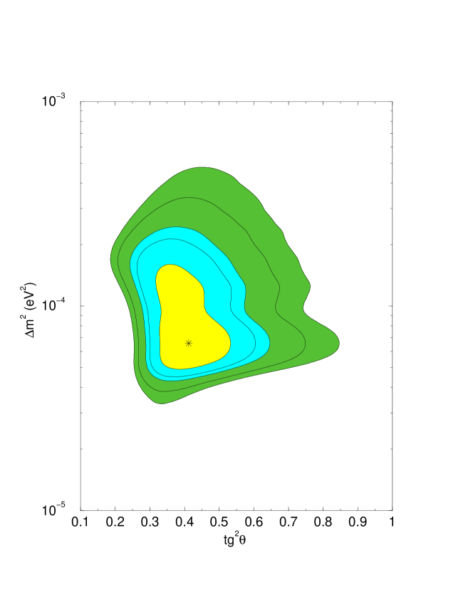
Figure 7: Three neutrino analysis with $\sin^{2}\theta_{13}=0.04$. The allowed regions in $\tan^{2}\theta-\Delta m^{2}$ from a combined fit of the solar neutrino data and the KamLAND rate at the 1$\sigma$, 90%, 95%, 99% and 3$\sigma$ C.L..

In fig. 7 we show results of the combined analysis of the solar data and the KamLAND rate. As can be concluded from comparison of fig. 3 and fig. 7, the main impact of non-zero 1-3 mixing is a slight shift of the allowed region to larger $\Delta m^{2}$ and smaller $\tan^{2}\theta$. In particular, we find that the best fit, $\chi^{2}_{min}/d.o.f.=66.21/79$, is at

$$\Delta m^{2}=6.60\cdot 10^{-5}{\rm eV}^{2},~{}~{}~{}\tan^{2}\theta=0.411~{}~{}~{}f_{B}=1.08.$$ (26)

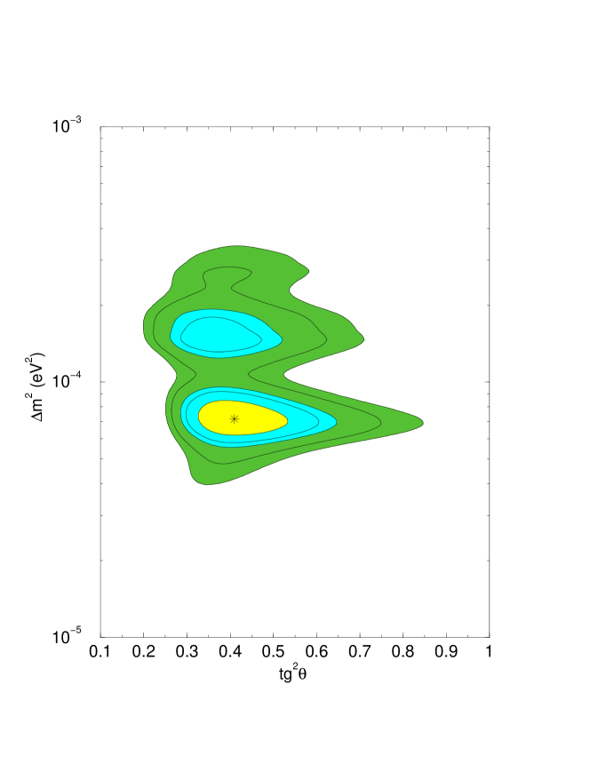
Figure 8: Three neutrino analysis with $\sin^{2}\theta_{13}=0.04$. The allowed regions in $\tan^{2}\theta-\Delta m^{2}$ plane from a combined analysis of the solar neutrino data and the KamLAND spectrum at the 1$\sigma$, 90%, 95%, 99% and 3$\sigma$ C.L..

In fig. 8 we show result of the combined analysis of the solar neutrino data and the KamLAND spectrum. From fig. 8 and fig. 4 we observe the same effect: 1-3 mixing leads to a shift of the allowed region to larger $\Delta m^{2}$ and smaller $\tan^{2}\theta$. In the best fit point we find $\chi^{2}_{min}/d.o.f.=69.24/91$ and

$$\Delta m^{2}=7.17\cdot 10^{-5}{\rm eV}^{2},~{}~{}~{}\tan^{2}\theta=0.41,~{}~{}f_{B}=1.07.$$ (27)

The introduction of the 1-3 mixing slightly worsen the fit: $\Delta\chi^{2}\approx 1$, it requires higher original boron neutrino flux, than in the $2\nu$- case. At the same time, the 1-3 mixing improves a fit in the h-region: It is accepted now at 90 % C.L. with respect to the best fit point (27). This region merges with the small spot at high $\Delta m^{2}$. The best fit point in the h-region is shifted to smaller mixing: $\tan^{2}\theta=0.36$.

For convenience, the results of different fits are summarized in the Table 1. It shows high stability of the extracted parameters with respect to a type of analysis.

Type of data fit	$\Delta m^{2}$	$\tan^{2}\theta$	$f_{B}$	$\chi^{2}_{min}$/d.o.f.
solar 2$\nu$	6.15	0.406	1.05	65.2/78
KL spectrum, 2$\nu$	7.34	0.453	-	2.92/11
solar + KL rate, 2$\nu$	6.03	0.411	1.05	65.3/79
solar + KL spectrum, 2$\nu$	7.32	0.409	1.05	68.2/91
solar + KL rate, 3$\nu$	6.60	0.411	1.08	66.2/79
solar + KL spectrum, 3$\nu$	7.17	0.409	1.07	69.2/91

Table 1: The parameters of the best fit points as well as $\chi^{2}_{min}/d.o.f.$ from different analyses of the data; $\Delta m^{2}$ is in the units $10^{-5}$ eV².

6 Next step

The key problems left after the first KamLAND results are

• more precise determination of the neutrino parameters: in particular, (i) precise determination of the deviation of 12-mixing from maximal mixing, (ii) strengthening of the upper bound on $\Delta m^{2}$ (iii) discrimination between the two existing regions;

• searches for effects beyond the single $\Delta m^{2}$ and single mixing approximation;

• searches for differences of the neutrino oscillation parameters determined from KamLAND and from the solar neutrino experiments.

Notice that precise knowledge of the parameters is crucial not only for the neutrinoless double beta decay searches, long baseline experiments, studies of the atmospheric and supernova neutrinos, etc., but also for understanding of physics of the solar neutrino conversion. In the region of the best fit point a dominating process (at least for $E>(0.5-1)$ MeV) is the adiabatic neutrino conversion (MSW), whereas in the high $\Delta m^{2}$ region allowed by KamLAND at the $2\sigma$ level, the effect is reduced to the averaged vacuum oscillations (a la Gribov-Pontecorvo) [29] with small matter corrections.

In this connection, we will discuss two questions.

How small $\Delta m^{2}$ can be? This is especially important question, e.g., for measurements of the earth regeneration effect. In the l-region we get

$$\Delta m^{2}>4\cdot 10^{-5}~{}~{}{\rm eV}^{2},~{}~{}~{}(3\sigma)$$ (28)

and it is difficult to expect that lower values will be allowed.

The bound (28) appears as an interplay of both the KamLAND rate and the shape. As it follows from the fig. 3, the KamLAND rate strengthens the lower bounds: $\Delta m^{2}\geq(3.0,~{}4.0,~{}4.7)\times 10^{-5}$ eV², at the $1\sigma$, $2\sigma$, $3\sigma$ correspondingly which should be compared with $\Delta m^{2}\geq(2.5,~{}3.2,~{}4.0)\times 10^{-5}$ eV² from the solar analysis only. Adding the spectral data results in the bounds $\Delta m^{2}\geq 3.3,~{}~{}5.5,~{}~{}6.2~{}~{}\times 10^{-5}$ eV²

With decrease of $\Delta m^{2}$ the oscillatory pattern of the spectrum shifts to lower energies. For $\Delta m^{2}=5\cdot 10^{-5}$ eV² the maximum of spectrum is at $E_{p}=2.7$ MeV and the oscillation suppression increases with energy [16]. The oscillation minimum is at $E_{p}\approx 5$ MeV. If $R_{KL}(2.7~{}{\rm MeV})=0.81$, then $R_{KL}(4.0~{}{\rm MeV})=0.47$. The KamLAND spectrum does not show such a fast decrease.

One can characterize the spectrum distortion by a relative suppression of signal at the high (say, above 4.3 MeV) and at the low (below 4.3 MeV) energies  . The energy interval (2.6 - 4.3) MeV contains KamLAND energy 4 bins. Introducing the suppression factors $R_{KL}(<4.3~{}{\rm MeV})$ and $R_{KL}(>4.3~{}{\rm MeV})$ we can define the ratio

$$k=\frac{1-R_{KL}(>4.3~{}{\rm MeV})}{1-R_{KL}(<4.3~{}{\rm MeV})}.$$ (29)

$k$ which we will call the shape parameter does not depend on the mixing angle and normalization of spectrum. It increases with increase of the oscillation suppression at high energies.

Using the KamLAND data we get the experimental value

$$k^{exp}=0.84^{+.42}_{-0.35},~{}~{}~{}1\sigma.$$ (30)

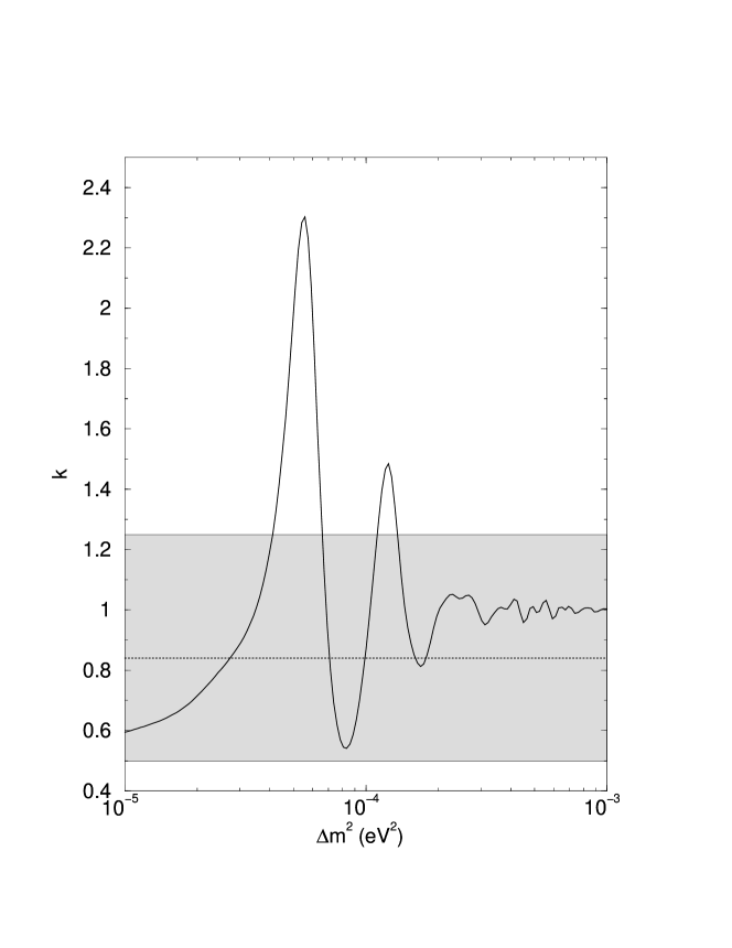
Figure 9: The dependence of the shape parameter $k$ on $\Delta m^{2}$ for $\tan^{2}\theta=0.41$. Shown are the central experimental value (dotted line) and the $1\sigma$ experimental band (shadowed).

In fig. 9 we present the dependence of the shape parameter $k$ on $\Delta m^{2}$ for fixed mixing: $\tan^{2}\theta=0.41$. For the spectrum which corresponds to the best combined fit we find $k=0.70$, whereas for $\Delta m^{2}=5\cdot 10^{-5}$ eV² the ratio equals $k=2.0$. For the h-region best point: $k=0.94$.

Notice that in the l-region below $\Delta m^{2}=8\cdot 10^{-5}$ eV², $k$ increases quickly with decrease of $\Delta m^{2}$, reaching a maximal value at $\Delta m^{2}=5.5\cdot 10^{-5}$ eV². Below that, the parameter $k$ decreases with $\Delta m^{2}$. In this region, however, the total event rate decreases fast giving the bound on $\Delta m^{2}$. This explains a shift of the allowed (at $3\sigma$) region to smaller mixings with decrease of $\Delta m^{2}$.

Notice also that the central experimental value of $k$ can be reproduced in the both allowed regions (l- and h-). Therefore future precise measurement of spectrum will further sharpen determination of $\Delta m^{2}$ within a given island. To discriminate among the islands one needs to use more elaborated criteria (not just $k$) or a complete spectral information.

How large is the large mixing? In contrast to [1] our best fit point is at non-maximal mixing $(\sin^{2}2\theta=0.86)$ being rather close to the best fit point from the solar neutrino analysis. Similar deviation from maximal mixing has been obtained in our rate+spectrum analysis. Notice that the KamLAND data have weak sensitivity to the mixing (weaker than the solar neutrino data). The allowed regions cover the interval

$$\tan^{2}\theta=0.12-1.00~{}~{}~{}~{}~{}(\theta<\pi/2),~{}~{}~{}~{}95\%{\rm C.L.}.$$ (31)

Even at $1\sigma$ the interval $\tan^{2}\theta=0.23-1.00$ $(\theta<\pi/2)$ is allowed. The reason is that KamLAND is essentially the vacuum oscillation experiment (see evaluation of matter effects in KamLAND in [23]), and effects of the vacuum oscillations depend on deviation from maximal mixing which can be characterized by $\epsilon=(1/2-\sin^{2}\theta)$ quadratically: $P\propto 1-4\epsilon^{2}$. The matter conversion depends on $\epsilon$ linearly: $P\propto 1-2\epsilon$ [31].

Notice that maximal mixing is rather strongly disfavored by all measured solar neutrino rates. In the point indicated by KamLAND we predict the charged current to neutral current measurement at SNO, the Argon production rate and the Germanium production rate:

$$\frac{\rm CC}{\rm NC}=0.51~{}(+3.3\sigma),~{}~{}~{}Q_{Ar}=3.2~{}{\rm SNU}~{}(+2.5\sigma),~{}~{}~{}Q_{Ge}=63~{}{\rm SNU}~{}(-1.6\sigma).$$ (32)

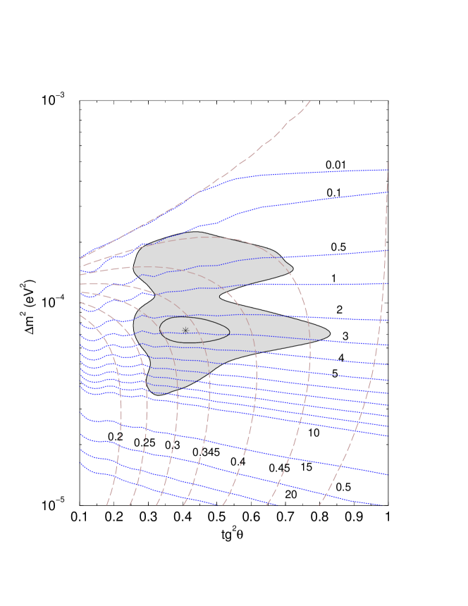
Figure 10: Predictions for the CC/NC ratio and the Day-Night asymmetry at SNO. The dashed lines are the lines of constant CC/NC ratio (numbers at the curves) and the dotted lines show the lines of constant $A_{DN}^{SNO}$ (numbers at the curves in %). We show also the ($1\sigma$ and $3\sigma$) allowed regions of the oscillation parameters from the combined fit of the solar neutrino data and the KamLAND spectrum. The best fit point is indicated by a star.

In brackets we show the pulls of the predictions from the best fit experimental values. As follows from the fig. 10 future precise measurements of the CC/NC ratio at SNO will strengthen the upper bounds on both mixing and $\Delta m^{2}$.

It is important to “overdetermine” the neutrino parameters measuring all possible observables. This will allow us to make cross-checks of selected solution and to search for inconsistencies which will require extensions of the theoretical context. In this connection let us consider predictions for the forthcoming measurements.

1). Precise measurements of the CC/NC ratio at SNO. In fig. 10 we show the contours of constant CC/NC ratio. We find predictions for the best fit point and the $3\sigma$ interval:

$$\frac{\rm CC}{\rm NC}=0.33^{+0.15}_{-0.07}~{},~{}~{}~{}3\sigma.$$ (33)

At $99\%$ C.L. the islands split and we get the following predictions for them separately:

$$\frac{\rm CC}{\rm NC}({\rm l-region})=0.33^{+0.11}_{-0.06}~{},~{}~{}~{}~{}\frac{\rm CC}{\rm NC}({\rm h-region})=0.38^{+0.06}_{-0.03}~{},~{}~{}~{}~{}~{}~{}~{}~{}99\%~{}{\rm C.L.}~{}.$$ (34)

Values of CC/NC $<0.35$ will exclude the h-region. Precise measurements of the ratio CC/NC will also strengthen the upper bounds on mixing and $\Delta m^{2}$.

2). The day-night asymmetry at SNO. The KamLAND provides a strong lover bound on $\Delta m^{2}$, and shifts the best fit point to larger $\Delta m^{2}$. This further diminishes the expected value of day-night asymmetry. In fig. 10 we show the contours of constant $A_{DN}^{SNO}$. The best fit point prediction and the $3\sigma$ bound equal

$$A_{ND}^{SNO}=2.8\pm 0.8\%~{},~{}~{}~{}(1\sigma),~{}~{}~{}~{}~{}A_{ND}^{SNO}<9\%~{}~{}~{}~{}(3\sigma).$$ (35)

The present best fit value of the SNO asymmetry, $7\%$, is accepted at about 99% C.L.. Observations of the asymmetry $A_{ND}^{SNO}>1\%$ will exclude the h-region. The expected asymmetry at Super-Kamiokande is even smaller: In the best fit point we expect $A_{ND}^{SK}\approx(1.7-2.0)\%$.

3). The turn up of the spectrum at SNO and Super-Kamiokande at low energies. Using results of [32] we predict for the best fit point (18) an increase of ratio of the observed to expected (without oscillation) number of the CC events, $R_{SNO}^{CC}$, from 0.31 at 8 MeV to 0.345 at 5 MeV, so that

$$\frac{R_{SNO}^{CC}({\rm 5MeV})-R_{SNO}^{CC}({\rm 8MeV})}{R_{SNO}^{CC}({\rm 8MeV})}=0.10-0.12.$$ (36)

In Super-Kamiokande the turn up is about $(5-7)\%$ in the same interval (5 - 8) MeV.

4). Further KamLAND measurements. Possible impact can be estimated using figures 1, 2, 5. A decrease of the error by factor of 2 (which will require both significant increase of statistics and decrease of the systematic error) will allow KamLAND alone to exclude all the regions but the l-region at 95 % C.L., if the best fit is at the same point as it is determined now.

5). BOREXINO. At $3\sigma$ we predict the following suppressions of signals with respect to the SSM predictions to BOREXINO experiment [33], in the two allowed regions:

$$R_{B}({\rm l-region})=0.61-0.73,~{}~{}~{}R_{B}({\rm h-region})=0.62-0.73.$$ (37)

So, BOREXINO will perform consistency check but it will not distinguish the l- and h- regions.

6). Gallium production rate. In the best fit point one predicts the germanium production rate $Q_{Ge}=71$ SNU. In the h-region best fit point $Q_{Ge}=72$ SNU. So, the Gallium experiments do not discriminate among the l - and h - regions. However, precise measurements of $Q_{Ge}$ are important for improvements of the bound on the 1-2 mixing and its deviation from maximal value.

7 Conclusions

1. The first KamLAND results (rate and spectrum) are in a very good agreement with the predictions based on the LMA MSW solution of the solar neutrino problem.

2. Our analysis of the KamLAND data reproduces well the results of the collaboration. The oscillation parameters extracted from the KamLAND data and from the solar neutrino data agree within $1\sigma$.

3. We have performed a combined analysis of the solar and KamLAND results. The main impact of the KamLAND results on the LMA solution can be summarized in the following way. KamLAND

• shifts the $\Delta m^{2}$ to slightly higher values $6.15\cdot 10^{-5}$ $\rightarrow 7.3\cdot 10^{-5}$ eV²; (the mixing is practically unchanged: $\tan^{2}\theta=0.41$, and this number is rather stable with respect to variations of the analysis;

• establishes rather solid lower bound on the $\Delta m^{2}$: $\Delta m^{2}>4\cdot 10^{-5}$ eV² ($3\sigma$);

• disintegrates the LMA region at 99% C.L. into two parts.

KamLAND further disfavors high values of $\Delta m^{2}$: $\Delta m^{2}>3\cdot 10^{-4}$ eV².

4. Inclusion of the 1-3 mixing shifts the allowed regions to larger $\Delta m^{2}$ and smaller $\tan^{2}\theta$. $\chi^{2}$ slightly increases with $\sin^{2}\theta_{13}$.

5. The KamLAND results strengthen the upper bound on the expected value of the day-night asymmetry at SNO: $A_{DN}^{SNO}<9\%$. We predict about 10% turn up of the energy spectrum at SNO in the interval of energies (5 - 8) MeV. The CC/NC ratio is expected to be CC/NC $\approx 0.33$, that is, near the present best SNO value.

Future SNO measurements of the CC/NC ratio and $A_{DN}^{SNO}$ will have further strong impact on the LMA parameter space.

8 Acknowledgments

The authors are grateful to E. Kh. Akhmedov for useful discussions.

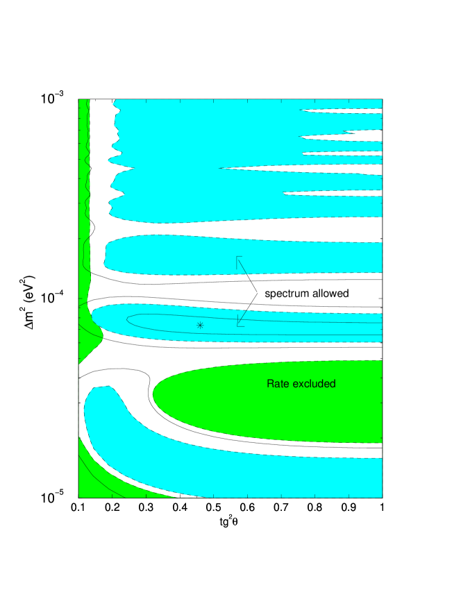
Figure 1: The KamLAND spectrum analysis for $E_{p}>2.6$ MeV. Shown are the allowed regions of oscillation parameters at 68% (inner solid lines), 95% (grey) and 99% C.L. (outer solid lines). The best fit point is indicated by star. Also shown are the regions excluded by the rate analysis at $95\%$ C.L. (dark).

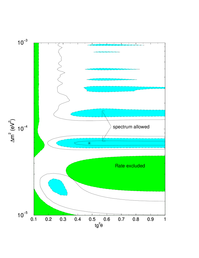
Figure 2: The same as in fig. 1 for $E_{p}>0.9$ MeV.

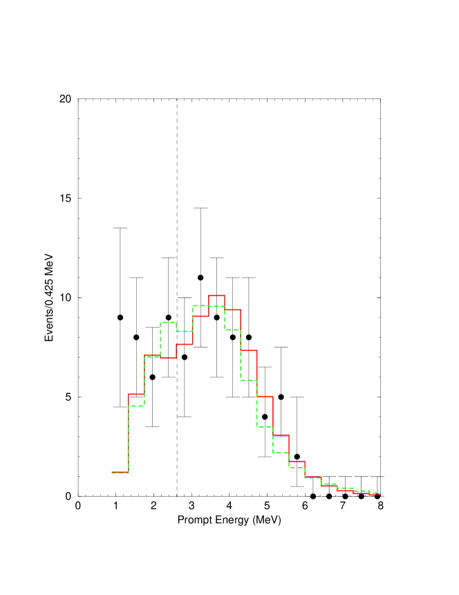
Figure 5: The expected prompt energy spectra for the best fit points from the l-region (solid histogram) and h-region (dashed histogram). Also shown are the KamLAND experimental points.

References

- [1] K. Eguchi et al., KamLAND collaboration, hep-ex/0212021.
- [2] J. N. Bahcall, “Neutrino astrophysics”, Cambridge U. Press, Cambridge, England, 1989.
- [3] L. Wolfenstein, Phys. Rev. D 17, 2369 (1978); S. P. Mikheyev and A. Yu. Smirnov, Yad. Fiz. 42, 1441 (1985) [ Sov. J. Nucl. Phys. 42, 913 (1985)], Nuovo Cim. C9, 17 (1986); S. P. Mikheyev and A. Yu. Smirnov, ZHETF, 91, (1986), [Sov. Phys. JETP, 64, 4 (1986)].
- [4] The triangle (at least its horizontal and diagonal sides) appears already in the first publications [3], see also S. P. Rosen, J. M. Gelb, Phys. Rev. D34, 969 (1986), W.C. Haxton, Phys. Rev. Lett. 57, 1271 (1986). The complete triangle with the vertical side included had been constructed independently by J. Bouches et al., Proc. of the 6th Moriond Workshop on Massive Neutrinos in Astrophysics and Particle Physics, (Tignes, France) eds. O. Fackler and J. Tran Thanh Van, 129, (1986); S. J. Parke, Phys. Rev. Lett. 57, 1275 (1986); S. P. Mikheyev and A. Yu. Smirnov, Proc. of the 12th Int. Conf Neutrino’86 (Sendai, Japan) eds. T. Kitagaki and H. Yuta, 177 (1986) and Proc. of the Int. Symp. on Weak and Electromagnetic Interactions in Nuclei, WEIN-86, (Heidelberg, 1986), 710; M. Cribier et al., Phys. Lett. B182, 89 (1986); see also S. J. Parke and T. Walker, Phys. Rev. Lett. 57 2322 (1986).
- [5] B. T. Cleveland et al., Astroph. J. 496 (1998) 505; K. Lande et al., in Neutrino 2000 Sudbury, Canada 2000, Nucl. Phys. B (Proc. Suppl.) 50 (2001) 21. (Here and in ref. [7], [8], [9] we cite the latest publications of the collaboration in which the references to earlier works can be found.)
- [6] K. S. Hirata et al., Phys. Rev. Lett. 65 1297 (1990).
- [7] J.N. Abdurashitov et al. (SAGE collaboration), astro-ph/0204245.
- [8] T. Kirsten et al., Talk given at the 20th Int. Conf on Neutrino Physics and Astriphysics, Neutrino 2002, Munich, Germany, May 25 - 30, 2002.
- [9] S. Fukuda et al. (Super-Kamiokande collaboration) Phys. Rev. Lett. 86, 5651 (2001); Phys. Rev. Lett. 86, 5656 (2001).
- [10] J. N. Bahcall, P. I. Krastev, A. Yu. Smirnov, Phys. Rev. D60:093001 (1999).
- [11] M.C. Gonzalez-Garcia, P.C. de Holanda, C. Peña-Garay, J.W.F. Valle, Nucl. Phys. B573, 3 (2000).
- [12] Q. R. Ahmad et al., SNO collaboration, Phys. Rev. Lett. 87, 071301 (2001).
- [13] Q. R. Ahmad et al., SNO collaboration, Phys.Rev.Lett. 89:011301 (2002).
- [14] Q. R. Ahmad et al., SNO collaboration, Phys.Rev.Lett. 89:011302 (2002).
- [15] V. Barger, D. Marfatia, K. Whisnant, B.P. Wood, Phys. Lett. B537, 179 (2002); A. Bandyopadhyay, S. Choubey, S. Goswami, D. P. Roy, Phys. Lett. B540, 14 (2002); J. N. Bahcall, M.C. Gonzalez-Garcia, C. Peña-Garay, JHEP 0207:054, (2002); A. Strumia, C. Cattadori, N. Ferrari, F. Vissani, Phys.Lett. B541, 327 (2002); P. Aliani, V. Antonelli, R. Ferrari, M. Picariello, E. Torrente-Lujan, hep-ph/0205053; G.L. Fogli, E. Lisi, A. Marrone, D. Montanino, A. Palazzo, Phys. Rev. D66:053010, (2002); M. Maltoni, T. Schwetz, M.A. Tortola, J.W.F. Valle, hep-ph/0207227; M. Smy, hep-ex/0208004.
- [16] P. C. de Holanda, A. Yu. Smirnov, hep-ph/0205241, to be published in Phys. Rev. D.
- [17] J. N. Bahcall, M.H. Pinsonneault and S. Basu, Astrophys. J. 555 (2001) 990.
- [18] V. Barger, D. Marfatia, hep-ph/0212126.
- [19] G.L. Fogli, E. Lisi, A. Marrone, D. Montanino, A. Palazzo, A. M. Rotunno, hep-ph/0212127.
- [20] M. Maltoni, T. Schwetz, J.W.F. Valle, hep-ph/0212129.
- [21] P. Creminelli, G. Signorelli, A. Strumia, hep-ph/0102234, v.4, 9 Dec, (2002).
- [22] A. Bandyopadhyay, S. Choubey, Raj Gandhi, S. Goswami, D.P. Roy, hep-ph/0212146.
- [23] J. N. Bahcall, M.C. Gonzalez-Garcia, C. Peña-Garay, hep-ph/0212147.
- [24] H. Nunokawa, W. J. C. Teves, R. Zukanovich Funchal, hep-ph/0212202.
- [25] P. Aliani, V. Antonelli, M. Picariello, E. Torrente-Lujan, hep-ph/0212212.
- [26] L. E. Marcucci et al., Phys. Rev. C63 (2001) 015801; T.-S. Park, et al., nucl-th/0107012, nucl-th/0208055 and references therein.
- [27] M.C. Gonzalez-Garcia, C. Peña-Garay, Phys. Lett. B527:199 (2002).
- [28] CHOOZ Collaboration, M. Apollonio et al., Phys.Lett. B420, 397 (1998).
- [29] V. N. Gribov and B. Pontecorvo, Phys. Lett. B28, 493 (1969).
- [30] J. N. Bahcall, M.C. Gonzalez-Garcia, C. Peña-Garay, in [15].
- [31] M. C. Gonzalez-Garcia, C. Peña-Garay, Y. Nir, A. Yu. Smirnov, Phys. Rev. D63:013007 (2001).
- [32] P.I. Krastev, A.Yu. Smirnov, Phys. Rev. D65:073022 (2002).
- [33] BOREXINO Collaboration, G. Alimonti et al., Astropart. Phys. 16 (2002) 205.