TRANSPORT COEFFICIENTS AND QUANTUM FIELDS

Abstract

Various aspects of transport coefficients in quantum field theory are reviewed. We describe recent progress in the calculation of transport coefficients in hot gauge theories using Kubo formulas, paying attention to the fulfillment of Ward identities. We comment on why the color conductivity in hot QCD is much simpler to compute than the electrical conductivity. The nonperturbative extraction of transport coefficients from lattice QCD calculations is briefly discussed.

1 Introduction

Transport coefficients characterize the response of a system in thermal equilibrium to a weak perturbation associated with a conserved current. Examples are the shear and bulk viscosities, electrical conductivity and diffusion constants. Transport coefficients can be relevant in various physical scenarios: in the formation and diffusion of large-scale magnetic fields[1], in compact stars[2] and in relativistic heavy-ion collisions[3].

The calculation of transport coefficients in thermal field theory through Kubo formulas turns out to be highly nontrivial. The main problem is that already at leading-logarithmic order an infinite class of diagrams, known as ladder diagrams, has to be summed. This has favored the use of kinetic theory where a few scattering amplitudes must be included in the collision term. It is within the kinetic approach that it was first realized that screening processes are necessary and sufficient to obtain finite transport coefficients[4] and a complete leading-log calculation for a variety of transport coefficients has appeared a few years ago[5].

However, recent work[6] has contributed to establish an efficient and easy way to compute transport coefficients to leading-log order using the imaginary-time formalism of thermal field theory in a way that is consistent with the Ward identity[7]. In the following we focus on these developments, describing the leading-log calculation of the electrical conductivity. After that we comment on why the nonabelian color conductivity turns out to be a much simpler quantity to compute. Finally we discuss the use of lattice QCD as a nonperturbative approach to the calculation of transport coefficients.

2 Electrical conductivity

In linear response theory transport coefficients are written as equilibrium expectation values of commutators of currents. Indeed, the Kubo formula for the electrical conductivity in QED is

$$\sigma=\lim_{q^{0}\to 0}\frac{1}{3}\,\frac{\partial}{\partial q^{0}}{\mathrm{Im}}\,\Pi^{ii}_{R}(q^{0},{\mathbf{0}}),$$ (1)

where the retarded polarization tensor and electromagnetic current are

$$\Pi^{\mu\nu}_{R}(x-y)=i\theta(x^{0}-y^{0})\langle[j^{\mu}(x),j^{\nu}(y)]\rangle,\;\;\;\;\;\;j^{\mu}(x)=\bar{\psi}(x)\gamma^{\mu}\psi(x).$$ (2)

At weak coupling one might naively expect a one-loop calculation to be sufficient and such a calculation yields

$$\sigma=-\frac{2e^{2}}{3}\int_{{\mathbf{p}},\omega}n_{F}^{\prime}(\omega)\left[\Delta^{R}_{+}(\omega,{\mathbf{p}})\Delta^{A}_{+}(\omega,{\mathbf{p}})+\Delta^{R}_{-}(\omega,{\mathbf{p}})\Delta^{A}_{-}(\omega,{\mathbf{p}})\right],$$ (3)

where $\int_{\mathbf{p}}=\int d^{3}p/(2\pi)^{3}$, $\int_{\omega}=\int d\omega/(2\pi)$ and $n_{F}$ is the Fermi distribution function. Here $\Delta^{R}_{\pm}$ denotes the retarded particle/anti-particle propagator and $\Delta^{A}_{\pm}$ the corresponding advanced one. These scalar propagators were introduced by decomposing the fermion propagator as

$$S(\omega,{\mathbf{p}})=\Delta_{+}(\omega,{\mathbf{p}})h_{+}(\hat{{\mathbf{p}}})+\Delta_{-}(\omega,{\mathbf{p}})h_{-}(\hat{{\mathbf{p}}}),$$ (4)

with $h_{\pm}(\hat{{\mathbf{p}}})=(\gamma^{0}\mp\boldsymbol{\gamma}\cdot\hat{{\mathbf{p}}})/2$, $\hat{{\mathbf{p}}}={\mathbf{p}}/p$, and here and below we neglect the zero temperature electron mass for fermions with momentum $p=|{\mathbf{p}}|\sim T$. In the free theory the scalar propagators are

$$\Delta^{R}_{\pm,\rm free}(\omega,{\mathbf{p}})=\frac{-1}{\omega\mp p+i0^{+}}=\left[\Delta^{A}_{\pm,\rm free}(\omega,{\mathbf{p}})\right]^{*}.$$ (5)

Since the free retarded (advanced) propagator has a pole at $\omega=\pm p$ approaching the real axis from below (above), the products of the retarded and advanced propagators as they appear in Eq. (3) suffer from so-called pinching poles: the integration over the energy variable in Eq. (3) is ill-defined and the naive result for the conductivity is infinity!

This particular result is of course well-known[8, 9] and has two major consequences. One has to

• include a thermal width,

• include an infinite series of ladder diagrams like the one in Fig. 1.

Figure 1: Typical ladder diagram that contributes to the electrical conductivity at leading-logarithmic order. The side rails represent hard nearly on-shell fermions, dressed with a width, and the rungs are soft (HTL resummed) photons.

The inclusion of the thermal width $\Gamma_{\mathbf{p}}$ modifies the retarded and advanced single-particle propagators, which now read

$$\Delta^{R}_{\pm}(\omega,{\mathbf{p}})=\frac{-1}{\omega\mp p+i\Gamma_{{\mathbf{p}}}/2}=\left[\Delta^{A}_{\pm}(\omega,{\mathbf{p}})\right]^{*}.$$ (6)

As a result the pinching poles are screened (the distance between the poles is finite, namely $\Gamma_{\mathbf{p}}$), which makes Eq. (3) well-defined. Indeed, the products of the retarded and advanced propagators are now

$$\Delta^{R}_{\pm}(\omega,{\mathbf{p}})\Delta^{A}_{\pm}(\omega,{\mathbf{p}})=\frac{1}{(\omega\mp p)^{2}+(\Gamma_{{\mathbf{p}}}/2)^{2}}\longrightarrow\frac{2\pi}{\Gamma_{{\mathbf{p}}}}\delta(\omega\mp p),$$ (7)

where the last equation is valid in the limit of weak coupling.

The second consequence, the need to sum all ladders, is technically more involved. For the shear viscosity in scalar field theory this feature has been first recognized and implemented in full detail by Jeon[9]. His analysis has subsequently been confirmed and simplified by a number of groups[10]. For gauge theories the problem was realized by Lebedev and Smilga[8] ten years ago, but no complete calculation has been provided. Mottola and Bettencourt[11] have discussed the possibility of extracting the electrical conductivity from a consistent truncation of the Schwinger-Dyson hierarchy, but again without presenting a complete calculation.

This unsatisfactory situation for gauge theories changed only recently when Valle Basagoiti[6] used a concise method to sum ladder diagrams, borrowing techniques from the condensed-matter literature, and obtained equations for the shear viscosity and electrical conductivity to leading-logarithmic order in (non)abelian gauge theories that are equivalent to those obtained before using effective kinetic theory[5]. One way to sum all the ladders diagrams for the electrical conductivity in QED is to introduce an effective electron-photon vertex defined by an integral equation whose formal solution is the geometric series summing all the rungs in the ladder. Although the method presented by Valle Basagoiti solved in a simple way the problem of summing the ladder series, his treatment missed one important point since his integral equation was not consistent with the Ward identity. Indeed, in order to fulfill the Ward identity an additional diagram has to be included in the equation for the effective vertex[7] and the correct integral equation is depicted in Fig. 2 (the second diagram on the RHS is the new necessary element). However, although this extra diagram is essential to fulfill the Ward identity, it does not contribute to the conductivity at leading-log order[7]. These results have been confirmed recently[12].

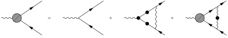
Figure 2: Integral equation for the effective electron-photon vertex, $\Gamma^{\mu}=\gamma^{\mu}+\Gamma^{\mu}_{\rm HTL}+\Gamma^{\mu}_{\rm ladder}$. The HTL propagators and vertices are indicated with black blobs. The external photon has zero momentum and vanishing energy. Other lines represent hard nearly on-shell particles.

Using the techniques previously mentioned[6] the complete expression for the electrical conductivity at leading-log order can now be written in a way that closely resembles the one-loop result. It reads

$$\sigma=-\frac{2}{3}e^{2}\int_{{\mathbf{p}},\omega}n_{F}^{\prime}(\omega)\big{[}\Delta^{R}_{+}(\omega,{\mathbf{p}})\Delta^{A}_{+}(\omega,{\mathbf{p}})\,\hat{p}^{i}\,{\mathrm{Re}}\,D_{+}^{i}(\omega,\omega;{\mathbf{p}})$$

$$-\Delta^{R}_{-}(\omega,{\mathbf{p}})\Delta^{A}_{-}(\omega,{\mathbf{p}})\,\hat{p}^{i}\,{\mathrm{Re}}\,D_{-}^{i}(\omega,\omega;{\mathbf{p}})\big{]},$$ (8)

where we defined

$$D^{\mu}_{+}(\omega+q^{0},\omega;{\mathbf{p}}) \equiv \bar{u}_{\lambda}(\hat{{\mathbf{p}}})\Gamma^{\mu}(\omega+q^{0}+i0^{+},\omega-i0^{+};{\mathbf{p}})u_{\lambda}(\hat{{\mathbf{p}}}),$$ (9)

$$D^{\mu}_{-}(\omega+q^{0},\omega;{\mathbf{p}}) \equiv \bar{v}_{\lambda}(\hat{{\mathbf{p}}})\Gamma^{\mu}(\omega+q^{0}+i0^{+},\omega-i0^{+};{\mathbf{p}})v_{\lambda}(\hat{{\mathbf{p}}}).$$ (10)

$\Gamma^{\mu}$ represents the effective vertex and $u_{\lambda}$ ($v_{\lambda}$) are spinors for the electron (positron) in a simultaneous chirality-helicity base. Since the conductivity is dominated by the pinching-pole contribution, out of the many different electron-photon vertices $\Gamma^{i}$ with real energies[13] only one particular analytical continuation contributes. Recalling Eq. (7), it is convenient to define

$${\mathcal{D}}(p)\equiv\pm\hat{p}^{i}{\mathrm{Re}}\,D^{i}_{\pm}(\pm p,\pm p;{\mathbf{p}}),$$ (11)

where we made use of rotational invariance and CP properties of the vertex, and the electrical conductivity is given by

$$\sigma=-\frac{4e^{2}}{3}\int_{{\mathbf{p}}}n_{F}^{\prime}(p)\frac{{\mathcal{D}}(p)}{\Gamma_{{\mathbf{p}}}}.$$ (12)

The 4 arises from electrons and positrons with either helicity that contribute in the same way to the conductivity.

3 Ward identity

The diagrammatic evaluation of transport coefficients has two main ingredients: the inclusion of the thermal width which modifies the propagator and the summation of an infinite series of ladder diagrams which modifies the electron-photon vertex. In a gauge theory these two features have to be related, since the propagator and the vertex are connected through the Ward identity

$$Q_{\mu}\Gamma^{\mu}(P+Q,P)=S^{-1}(P)-S^{-1}(P+Q).$$ (13)

For the specific situation we are considering, the Ward identity reads

$$q^{0}\Gamma^{0}(p^{0}+q^{0}+i0^{+},p^{0}-i0^{+};{\mathbf{p}})=q^{0}\gamma^{0}+\Sigma^{A}(p^{0},{\mathbf{p}})-\Sigma^{R}(p^{0}+q^{0},{\mathbf{p}}),$$ (14)

in the special kinematical regime relevant for the conductivity, i.e. $q^{0}\to 0$ and $p^{0}\simeq\pm p$. In terms of the quantity

$${\mathfrak{D}}({\mathbf{p}})\equiv\lim_{q^{0}\to 0}q^{0}D_{\pm}^{0}(\pm p+q^{0},\pm p;{\mathbf{p}}),$$ (15)

the Ward identity takes a particularly simple form

$$\mathfrak{D}({\mathbf{p}})=i\Gamma_{\mathbf{p}}.$$ (16)

Since only the imaginary part of the self-energy is resummed, the RHS of the equation above is purely imaginary. From the definition in Eq. (15) it is clear that the imaginary part of the vertex should diverge as $1/q^{0}$ when $q^{0}\to 0$. We want to verify that the Ward identity is indeed satisfied, by computing both sides of Eq. (16) independently.

The thermal width $\Gamma_{\mathbf{p}}$ of an on-shell electron with hard momentum can be computed from the imaginary part of the self-energy. The leading terms with logarithmic sensitivity to the coupling constant arise from the diagrams shown in Fig. 3, with $\Gamma_{\mathbf{p}}=\Gamma_{\mathbf{p}}^{\rm(sp)}+\Gamma_{\mathbf{p}}^{\rm(sf)}$.

(sp)                                (sf)

Figure 3: Contributions to the thermal width of a hard on-shell fermion from a soft photon (sp) and a soft fermion (sf).

The soft-photon contribution can be written as $\Gamma_{\mathbf{p}}^{\rm(sp)}=\Gamma_{\mathbf{p}}^{\rm(sp,lo)}+\Gamma_{\mathbf{p}}^{\rm(sp,nlo)}$ for the first two terms with logarithmic sensitivity. The explicit expressions are[14, 7]

$$\Gamma_{\mathbf{p}}^{\rm(sp,lo)} = 2\alpha T\ln(m_{D}/\Lambda_{\rm min}),$$ (17)

$$\Gamma_{\mathbf{p}}^{\rm(sp,nlo)} = \frac{\alpha\,m_{D}^{2}\ln(1/e)}{2p}\left[-1+2n_{F}(p)+\frac{p}{6T}+2p\,n_{F}^{\prime}(p)\right],$$ (18)

where $\alpha=e^{2}/4\pi$ and $m_{D}=eT/\sqrt{3}$ is the Debye mass. The leading-log contribution from soft fermions is[6, 7]

$$\Gamma^{\rm(sf,lo)}_{{\mathbf{p}}}=\frac{\alpha\,m_{f}^{2}\ln(1/e)}{p}\left[1+2n_{B}(p)\right],$$ (19)

with $m_{f}=eT/\sqrt{8}$ the fermionic thermal mass and $n_{B}$ the Bose distribution function. The technical reason why one needs to include the next “logarithmic” order is that just doing a naive leading-log order calculation (i.e. keeping only $\Gamma_{\mathbf{p}}^{\rm(sp,lo)}$) leads to an integral equation without solution. We demonstrate this below. Furthermore, $\Gamma_{\mathbf{p}}^{\rm(sp,lo)}$ is actually ill-defined[14] and diverges logarithmically; $\Lambda_{\rm min}$ is an ad-hoc infrared cut-off introduced to regulate the divergence. It is then clear that for the method to be meaningful any dependence on this piece of the thermal width must disappear in the end. The physical reason is that the electrical conductivity is determined by large-angle Coulomb scattering along with pair annihilation and Compton scattering[5]: this sets the relevant scale to be $e^{4}T\ln(T/m_{D})$. The leading term in the thermal width, however, arises from the exchange of ultrasoft quasistatic gauge bosons which corresponds to small-angle scattering. Processes which give the next “logarithmic” order of the thermal width (as can be seen by cutting the diagrams) are precisely those related to the scale $e^{4}T\ln(T/m_{D})$; in the soft-fermion case directly through the thermal width $\Gamma^{\rm(sf,lo)}_{{\mathbf{p}}}$ and in the soft-photon case in a more subtle way through the integration over the rung in the integral equation. It is therefore understandable (of course, now that both the underlying physics and the technical details are known) that subleading terms in the thermal width must be included and that the dependence on the leading one in the end should disappear. We will see how this works in detail in the next section.

We now to turn to verify that our integral equation $\Gamma^{0}=\gamma^{0}+\Gamma^{0}_{\rm HTL}+\Gamma^{0}_{\rm ladder}$ (see Fig. 2) is consistent with the Ward identity. It can be checked in detail[7], but here we will just argue that Eq. (13) makes it natural to expect that the inclusion of a contribution to the self-energy with soft fermion lines must go with a corresponding contribution to the vertex. The correspondence is shown in Fig. 4.

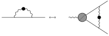
$\Gamma_{\mathbf{p}}^{\rm(sp)}$                    $\Gamma^{0}_{\rm ladder}$              $\Gamma_{\mathbf{p}}^{\rm(sf)}$                       $\Gamma^{0}_{\rm HTL}$

Figure 4: The imaginary parts of the fermion self-energy and the two terms in the integral equation for the electron-photon vertex are directly related to each other via the Ward identity. The self-energy with a soft photon (sp) corresponds in the effective vertex to the term that leads to the infinite series of ladder diagrams, the self-energy with a soft fermion (sf) corresponds to a vertex correction with HTL vertex and propagators.

The contribution of $\Gamma^{0}_{\rm ladder}$ to $\mathfrak{D}({\mathbf{p}})$ is precisely the soft-photon contribution to the thermal width, while the new diagram $\Gamma^{0}_{\rm HTL}$ is precisely the required piece to obtain the soft-fermion part of the $\Gamma_{{\mathbf{p}}}$. Therefore, the inclusion of the thermal width and the summation of ladder diagrams are in fact closely related and one cannot do one without the other. This is relevant for computations beyond leading-log: any additional diagram that contributes to the thermal width should be reflected in corresponding new contributions to the integral equation for the effective vertex and vice versa.

4 Leading-log result

To obtain the final result for the electrical conductivity the integral equation for the spatial part of the effective electron-photon vertex still has to be solved. Because only the real part of the effective vertex is needed, see Eq. (11), the calculation simplifies considerably since the real part of the new diagram $\Gamma_{\rm HTL}^{i}$ is subleading and therefore does not contribute[7].

The integral equation for the vertex ${\mathcal{D}}(p)$ can be written as[7]

$${\mathcal{D}}(p)=1+\frac{\alpha}{2p^{2}}\int_{\Lambda_{\rm min}}^{\Lambda_{\rm max}}\!\!\!\!\!\!dk\,k\int_{-k}^{k}\frac{d\omega}{2\pi}\left[n_{B}(\omega)+n_{F}(p+\omega)\right]\left\{\hat{{\mathbf{p}}}\cdot\hat{{\mathbf{r}}}\frac{{\mathcal{D}}(r)}{\Gamma_{{\mathbf{r}}}}\Big{|}_{z=z_{0}}\right\}$$

$$\times\left[{}^{\ast}\!\rho_{T}(\omega,k)\frac{k^{2}-\omega^{2}}{k^{2}}\left[(\omega+2p)^{2}+k^{2}\right]+{}^{\ast}\!\rho_{L}(\omega,k)\left[(\omega+2p)^{2}-k^{2}\right]\right].$$ (20)

Here ${}^{\ast}\!\rho_{T/L}(\omega,k)$ are the spectral densities for the soft transverse/longitudinal photons in the rung, ${\mathbf{r}}={\mathbf{p}}+{\mathbf{k}}$, $z=\hat{{\mathbf{k}}}\cdot\hat{{\mathbf{p}}}$, and $z_{0}=\omega/k+(\omega^{2}-k^{2})/(2pk)$. $\Lambda_{\rm max}$ is an upper cut off introduced to be consistent with the condition that the photon carries soft momentum; at leading-log accuracy[15] it can be taken to be $T$. Save for the factor within braces, the integral is precisely the soft-photon contribution $\Gamma^{(\rm{sp})}_{{\mathbf{p}}}$ to the thermal width.

At this moment we can demonstrate the technical reason why keeping just the leading term $\sim e^{2}T$ to the thermal width is inconsistent. In the vertex equation the on-shell particles carry hard momentum $p$ and the collective HTL modes carry soft momentum $k$. This scale separation allows to expand the integrand in powers of $k/p$. At (naive) leading order, the term within the braces is just ${\mathcal{D}}(p)/\Gamma_{{\mathbf{p}}}$ and can be taken out of the integral. The integral equation then reduces to ${\mathcal{D}}(p)=1+{\mathcal{D}}(p)$ which has no solution!

We therefore proceed keeping subleading contributions to the width. In order to show that any dependence on the scale $\sim e^{2}T$ drops out, we write

$$\chi(p)=\frac{{\mathcal{D}}(p)}{\Gamma_{\mathbf{p}}},\;\;\;\;\;\;\sigma=-\frac{4e^{2}}{3}\int_{{\mathbf{p}}}n_{F}^{\prime}(p)\chi(p).$$ (21)

Expanding, as before, in powers of $k/p$ leads now to a differential equation for $\chi$, which with leading-log accuracy reads

$$1 = \frac{\alpha\,m_{f}^{2}\ln(1/e)}{p}\left[1+2n_{B}(p)\right]\chi(p)+\frac{\alpha\,m_{D}^{2}\ln(1/e)}{p}\frac{T}{p}$$ (22)

$$\times\left[\chi(p)-\left(1-\frac{p}{2T}\,[1-2n_{F}(p)]\right)p\,\chi^{\prime}(p)-\frac{1}{2}p^{2}\chi^{\prime\prime}(p)\right].$$

The only scale present in this equation is $e^{4}T\ln(1/e)$, as it should be. There is no dependence on $\Lambda_{\rm min}$. The parametrical dependence of the conductivity can be made explicit by writing

$$\chi(p)=\frac{T}{\alpha\,m_{D}^{2}\ln(1/e)}\,\phi(p/T),$$ (23)

such that

$$\sigma=C\frac{T}{e^{2}\ln(1/e)},\;\;\;\;\;\;\;\;\;\;\;\;\;\;C=\frac{2}{\pi}\int^{\infty}_{0}dy\,y^{2}\frac{1}{\cosh^{2}(y/2)}\phi(y),$$ (24)

and the dimensionless function $\phi(y)$ obeys the differential equation

$$1=\left[\frac{3\coth(y/2)}{8y}+\frac{1}{y^{2}}\right]\phi(y)+\left[\frac{1}{2}\tanh(y/2)-\frac{1}{y}\right]\phi^{\prime}(y)-\frac{1}{2}\,\phi^{\prime\prime}(y).$$ (25)

The integral in Eq. (24) is dominated by hard “momentum” $y=p/T$. In the limit of large $y$ the differential equation (25) simplifies considerably and is solved by the particular solution $\phi(y)=8y/7$. Using this approximate result yields

$$C_{\rm approx}=\frac{288}{7\pi}\zeta(3)\approx 15.7424,$$ (26)

which is close to the exact result $C=15.6964$, obtained by AMY[5] using a variational approach.

5 Soft fermions

As can be seen above, the relevant inverse time scale for the electrical conductivity is $\sim e^{4}T\ln(1/e)$. This scale enters the integral equation determining the effective vertex $\chi(p)$, see Eq. (22), and arises partly from the integration over the soft-photon rung and partly through the explicit appearance of the soft-fermion contribution to the thermal width (the first term on the RHS of Eq. (22)). Since in the diagrammatic calculation the soft-fermion contribution to the thermal width appears explicitly in the equation for the conductivity and since the imaginary part of the self-energy is directly related to scattering processes (as can be seen by cutting the diagrams), we expect that there is a direct relation between it and the inverse relaxation time from the corresponding scattering processes included in the collision term in the kinetic approach. The reason why we do not expect so with the soft-photon contribution is that it is ill-defined and the corresponding process contributes in a more subtle way to the integral equation, as explained above.

Figure 5: Scattering diagrams that contribute to the electrical conductivity at leading-logarithmic order in hot QED in kinetic theory (time runs horizontally).

The scattering processes that contribute to the electrical conductivity at leading-log order in kinetic theory[5] are shown in Fig. 5: large-angle Coulomb scattering (diagram C), pair creation/annihilation (D) and Compton scattering (E) (throughout this section we follow the notation of AMY[5]).

Since, as explained above, we are interested here in scattering processes where a soft fermion is exchanged, we restrict ourselves in the following to diagrams D and E. For two-to-two scattering processes the collision term reads

$$C[f]({\mathbf{p}})=\frac{1}{2}\int_{{\mathbf{k}},{\mathbf{k}}^{\prime},{\mathbf{p}}^{\prime}}\frac{\left|{\mathcal{M}}({\mathbf{p}},{\mathbf{k}};{\mathbf{p}}^{\prime},{\mathbf{k}}^{\prime})\right|^{2}}{2^{4}pp^{\prime}kk^{\prime}}(2\pi)^{4}\delta^{4}(P+K-P^{\prime}-K^{\prime})$$

$$\times\left\{f({\mathbf{p}})f({\mathbf{k}})[1\pm f({\mathbf{p}}^{\prime})][1\pm f({\mathbf{k}}^{\prime})]-f({\mathbf{p}}^{\prime})f({\mathbf{k}}^{\prime})[1\pm f({\mathbf{p}})][1\pm f({\mathbf{k}})]\right\},$$

where the $+/-$ signs refers to bosons/fermions. If the distribution function for the incoming fermion with momentum ${\mathbf{p}}$ is perturbed slightly away from equilibrium, $f({\mathbf{p}})=n_{F}({\mathbf{p}})+\delta f({\mathbf{p}})$, while all other distribution functions (bosonic and fermionic) are kept in equilibrium (i.e. using a relaxation-time approximation), the collision term can be written as

$$C[f]({\mathbf{p}})=\frac{1}{\tau_{\mathbf{p}}}\delta f({\mathbf{p}}),$$ (28)

with the inverse relaxation time given by

$$\frac{1}{\tau_{\mathbf{p}}}=\frac{1}{2(4\pi)^{4}p^{2}}\int^{T}_{eT}dq\int_{-q}^{q}d\omega\int_{0}^{\infty}dk\int_{0}^{2\pi}d\phi\,|{\mathcal{M}}|^{2}\,[\mbox{stat}.],$$ (29)

and $[\mbox{stat}.]$ is what remains of the statistical factors. Here $\omega=p^{\prime}-p$ and $q=|{\mathbf{p}}^{\prime}-{\mathbf{p}}|$ are the energy and momentum of the exchanged fermion and the integral over $q$ is cut off in the infrared by the expected Debye scale. Note that in the leading-log calculation using kinetic theory this is the only place where medium effects appear. To leading-log accuracy, one finds[5]

$$|{\mathcal{M}}|^{2}_{\rm D}=|{\mathcal{M}}|^{2}_{\rm E}=\frac{16e^{4}pk}{q^{2}}(1-\cos\phi),$$ (30)

and

$$\!\!\!\!\![\mbox{stat}.]_{\rm D}=n_{F}(k)[1+n_{B}(p)][1+n_{B}(k)]+n_{B}(p)n_{B}(k)[1-n_{F}(k)],$$ (31)

$$\!\!\!\!\![\mbox{stat}.]_{\rm E}=n_{B}(k)[1+n_{B}(p)][1-n_{F}(k)]+n_{B}(p)n_{F}(k)[1+n_{B}(k)].$$ (32)

The integrals in Eq. (29) can now be performed. To leading-log accuracy the relaxation rates associated with D and E are identical and the total relaxation rate corresponding to processes where a fermion is exchanged is, in the leading-log approximation,

$$\frac{1}{\tau_{\mathbf{p}}}\Big{|}_{\mbox{fermion exchanged}}=e^{4}\ln(1/e)\frac{T^{2}}{32\pi p}\left[1+2n_{B}(p)\right].$$ (33)

This is exactly the value of the soft-fermion contribution to the thermal width, see Eq. (19), as expected.

6 Color vs. electrical conductivity

It is instructive to compare the diagrammatic computation of the electrical conductivity with that of the color conductivity to leading-logarithmic order in hot QCD. The color conductivity appears in the effective theory describing the nonperturbative dynamics of ultrasoft modes of nonabelian gauge fields[16]. It was first computed within kinetic theory[17, 18] and it has also been obtained from a simplified ladder summation[19]. Although there is, as far as we know, no gauge invariant definition of this quantity, one can compute it diagrammatically using the nonabelian generalization of the Kubo formula (compare with Eq. (1)),

$$\sigma_{c}=\lim_{q^{0}\to 0}\frac{1}{3(N_{c}^{2}-1)}\frac{\partial}{\partial q^{0}}{\mathrm{Im}}\,\Pi_{iiR}^{aa}(q^{0},{\mathbf{0}}).$$ (34)

In principle one could think that the color conductivity is a more complicated quantity to compute than the electrical conductivity due to its nonabelian character. In reality the opposite is true. The reason is that the nonabelian nature of the interactions allows small-angle scattering to randomize the current by just changing the color charge of the current carriers[18]. This means that in this case it is sufficient to do a “real” leading-log calculation, i.e. it is enough to keep the leading-order term of the thermal width $\sim g^{2}T\ln(1/g)$. In a nonabelian theory the infrared logarithmic divergent behavior of this width is not a problem because there is natural mechanism to regulate it, the magnetic mass $m_{g}$.

We now outline the diagrammatic calculation of the leading-log order of the color conductivity, following[19], but using the exact and simplest way of carrying out the ladder summation. The calculation of the color conductivity goes along the same lines as the electrical conductivity. Since gluons are self-interacting there are both a quark and a gluon contribution. The integral equations are depicted in Fig. 6. We find (compare with Eq. (12))

$$\sigma_{c}=-\frac{4g^{2}}{3}\frac{N_{f}}{2}\int_{{\mathbf{p}}}n_{F}^{\prime}(p)\frac{{\mathcal{D}}_{\rm q}(p)}{\Gamma_{{\mathbf{p}}}^{\rm q}}-\frac{4g^{2}}{3}\frac{N_{c}}{2}\int_{{\mathbf{p}}}n_{B}^{\prime}(p)\frac{{\mathcal{D}}_{\rm g}(p)}{\Gamma_{{\mathbf{p}}}^{\rm g}},$$ (35)

where $N_{f}$ is the number of flavors. The quark-gluon effective vertex ${\mathcal{D}}_{\rm q}(p)$ is defined similarly to the electron-photon one, see Eq. (11). For the gluonic vertex we note that since the gluons on the side rails carry hard momentum the longitudinal contributions are exponentially suppressed and the gluon propagators are proportional to the transverse projector $P^{T}$. The gluon scalar function ${\mathcal{D}}_{\rm g}(p)$ is defined from the three-gluon effective vertex $\Gamma^{ijk}_{abc}$ after performing the analytical continuation, putting the hard gluons on the side rails on-shell, taking the energy $q^{0}$ of the external gluon to zero and contracting with transverse projectors, as

$$2f^{abc}p^{i}P^{T}_{jk}(\hat{{\mathbf{p}}})\,{\mathcal{D}}_{\rm g}(p)\equiv P^{T}_{kk^{\prime}}(\hat{{\mathbf{p}}})\,\Gamma^{ij^{\prime}k^{\prime}}_{abc}\,P^{T}_{jj^{\prime}}(\hat{{\mathbf{p}}}).$$ (36)

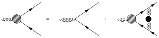
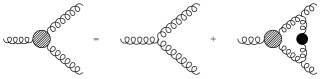
Figure 6: Integral equations for the effective quark-gluon vertex and three-gluon vertex, needed for the color conductivity at leading-logarithmic order.

As in the case of the electrical conductivity the ${\mathcal{D}}$’s represent the full vertex. The bare vertices correspond to ${\mathcal{D}}_{\rm q}(p)={\mathcal{D}}_{\rm g}(p)=1$. The leading-order thermal width of quarks resp. gluons is[20]

$$\Gamma_{{\mathbf{p}}}^{\rm q}=\frac{N_{c}^{2}-1}{2N_{c}}\,2\alpha_{s}T\ln(m_{D}/m_{g}),\;\;\;\;\;\;\Gamma_{{\mathbf{p}}}^{\rm g}=N_{c}\,2\alpha_{s}T\ln(m_{D}/m_{g}),$$ (37)

with $m_{g}\sim g^{2}T$ the magnetic mass and therefore $\ln(m_{D}/m_{g})\sim\ln(1/g)$.

It is now straightforward to adapt the calculation of the electrical conductivity to the problem at hand: the quark contribution to the color conductivity can easily be obtained just by inserting the correct group factors. The integral equation for the effective quark-gluon vertex is as in Eq. (4), with the substitutions: $\alpha\to-\alpha_{s}/(2N_{c})$ and $\Lambda_{\rm min}\to m_{g}$. At leading order in the expansion in $k/p$ the term within braces is just ${\mathcal{D}}_{\rm q}(p)/\Gamma_{{\mathbf{p}}}^{\rm q}$. It is independent of the integration variables and can be taken out of the integral. As we mentioned for the electrical conductivity, the remaining integral is just the thermal width, save for group factors in this case. The integral equation reduces therefore to an algebraic equation

$${\mathcal{D}}_{\rm q}(p)=1-\frac{1}{2N_{c}}\times\frac{{\mathcal{D}}_{\rm q}(p)}{\Gamma_{{\mathbf{p}}}^{\rm q}}\times\frac{2N_{c}}{N_{c}^{2}-1}\Gamma_{{\mathbf{p}}}^{\rm q}\;\;\;\;\Longrightarrow\;\;\;\;{\mathcal{D}}_{\rm q}(p)=1-\frac{1}{N_{c}^{2}}.$$ (38)

The calculation of the gluon contribution is quite similar and again the integral equation can be solved algebraically: the solution is ${\mathcal{D}}_{\rm g}(p)=2$.

Since neither the effective vertices nor the thermal widths depend on momentum, the final result for the color conductivity from Eq. (35) is

$$\sigma_{c}=\frac{g^{2}T^{2}}{9}\frac{N_{f}}{2}\frac{{\mathcal{D}}_{\rm q}}{\Gamma^{\rm q}}+\frac{g^{2}T^{2}}{9}N_{c}\frac{{\mathcal{D}}_{\rm g}}{\Gamma^{\rm g}}.$$ (39)

The ladder summation for the color conductivity is, as we see, substantially simpler than for other transport coefficients in hot gauge theories.

7 Transport coefficients from the lattice

Both kinetic and field theory allow to compute transport coefficients at high temperature, where the coupling constant is small. However, it would also be interesting to be able to compute transport coefficients at lower temperatures, where the coupling constant is no longer (very) small, which is relevant for heavy-ion collisions. In this section we discuss briefly the prospects[21, 22] of extracting transport coefficients at high temperature nonperturbatively from lattice QCD. As shown in Eq. (1) for the electrical conductivity, transport coefficients can defined from the slope of a spectral function $\rho(\omega,{\mathbf{0}})$ at vanishing energy ($\rho$ equals twice the imaginary part of the retarded correlator). Spectral functions can be related to euclidean-time correlators through a dispersion relation so that

$$G_{E}(\tau,{\mathbf{p}})=\int_{0}^{\infty}\frac{d\omega}{2\pi}\,K(\tau,\omega)\rho(\omega,{\mathbf{p}}),$$ (40)

with the kernel $K(\tau,\omega)=n_{B}(\omega)e^{-\omega\tau}+[1+n_{B}(\omega)]e^{\omega\tau}$. In the context of transport coefficients Eq. (40) has been employed first by Karsch and Wyld[23] and more recently by Nakamura et. al.[24] This approach consists of three steps:

• compute $G_{E}(\tau)$ (at zero momentum) numerically on the lattice,

• reconstruct $\rho(\omega)$ using either an ansatz[23] (old-fashioned approach) or the Maximal Entropy Method[25] (modern approach),

• extract the transport coefficient from the slope at vanishing energy.

Recently we have analyzed what can be expected in the context of the shear viscosity in scalar and nonabelian gauge theories at very high temperature[21] (the results can be adapted easily to other transport coefficients such as the electrical conductivity). We found that in a weakly-coupled field theory at high temperature the spectral function has a characteristic shape. In particular, there is a bump at very small energies which has its origin in the pinching singularities discussed above. The height of this bump at small energies is $\sim 1$ in units of the temperature.

The interesting question is how the spectral weight at small energies manifests itself in the euclidean correlator. For small energies $\omega\ll T$ the kernel can be expanded as $K(\tau,\omega)\simeq 2T/\omega+{\mathcal{O}}(\omega/T)$. Since all the $\tau$ dependence resides in the subdominant terms, the region relevant for transport coefficients contributes a single, constant term to the euclidean correlator: $G_{E}(\tau)\sim\int d\omega\,\rho(\omega)/\omega$. We find therefore that although euclidean correlators are sensitive to spectral weight at small energies in integrated form, they are, in weakly coupled theories, remarkably insensitive to further details of the spectral function in this region and, therefore, also to transport coefficients.

The findings about the small-energy region turn out to be rather generic[22]. They may therefore be relevant for recent attempts to reconstruct spectral functions at finite temperature in the high-temperature deconfined phase of QCD using the Maximal Entropy Method[26, 27].

8 Summary

We have reviewed several aspects of the diagrammatic calculation of transport coefficients in hot gauge theories to leading-log order. We focused in particular on recent progress within the imaginary-time formalism to sum the ladder series in an efficient way, on the importance of the Ward identity relating self-energy and vertex corrections, and on similarities and differences between the color and electrical conductivity. Finally, the prospects of extracting nonperturbative values for transport coefficients using lattice QCD were briefly mentioned.

References

- [1] See e.g. M. Giovannini, contribution to COSMO-01, hep-ph/0111220.
- [2] See e.g. M. G. Alford, contribution to ICHEP 2002, hep-ph/0209287.
- [3] See e.g. D. H. Rischke, contribution to “Hadrons in Dense Matter and Hadrosynthesis,” nucl-th/9809044.
- [4] G. Baym, H. Monien, C. J. Pethick and D. G. Ravenhall, Phys. Rev. Lett. 64 (1990) 1867.
- [5] P. Arnold, G. D. Moore and L. G. Yaffe, JHEP 0011 (2000) 001 [hep-ph/ 0010177].
- [6] M. A. Valle Basagoiti, Phys. Rev. D 66 (2002) 045005 [hep-ph/0204334].
- [7] G. Aarts and J. M. Martínez Resco, JHEP 0211 (2002) 022 [hep-ph/ 0209048].
- [8] V. V. Lebedev and A. V. Smilga, Physica A 181 (1992) 187.
- [9] S. Jeon, Phys. Rev. D 52 (1995) 3591 [hep-ph/9409250].
- [10] E. Wang and U. W. Heinz, Phys. Lett. B 471 (1999) 208 [hep-ph/9910367]; hep-th/0201116 (Phys. Rev. D, in press); M. E. Carrington, D. F. Hou and R. Kobes, Phys. Rev. D 62 (2000) 025010 [hep-ph/9910344].
- [11] E. Mottola and L. M. A. Bettencourt, in Proceedings of SEWM 2000.
- [12] D. Boyanovsky, H. J. de Vega and S. Y. Wang, hep-ph/0212107.
- [13] M. E. Carrington and U. W. Heinz, Eur. Phys. J. C 1 (1998) 619 [hep-th/9606055]; D. F. Hou and U. W. Heinz, ibid. 7 (1999) 101 [hep-th/9710090].
- [14] J. P. Blaizot and E. Iancu, Phys. Rev. D 55 (1997) 973 [hep-ph/9607303].
- [15] E. Braaten and T. C. Yuan, Phys. Rev. Lett. 66 (1991) 2183; E. Braaten and M. H. Thoma, Phys. Rev. D 44 (1991) 1298.
- [16] D. Bödeker, Phys. Lett. B 426 (1998) 351 [hep-ph/9801430].
- [17] A. Selikhov and M. Gyulassy, Phys. Lett. B 316 (1993) 373.
- [18] P. Arnold, D. T. Son and L. G. Yaffe, Phys. Rev. D 59 (1999) 105020 [hep-ph/9810216].
- [19] J. M. Martínez Resco and M. A. Valle Basagoiti, Phys. Rev. D 63 (2001) 056008 [hep-ph/0009331].
- [20] R. D. Pisarski, Phys. Rev. D 47 (1993) 5589.
- [21] G. Aarts and J. M. Martínez Resco, JHEP 0204 (2002) 053 [hep-ph/ 0203177].
- [22] G. Aarts and J. M. Martínez Resco, in Lattice 2002, hep-lat/0209033.
- [23] F. Karsch and H. W. Wyld, Phys. Rev. D 35 (1987) 2518.
- [24] A. Nakamura, S. Sakai and K. Amemiya, Nucl. Phys. Proc. Suppl. 53 (1997) 432 [hep-lat/9608052]; A. Nakamura, T. Saito and S. Sakai, ibid. 63 (1998) 424 [hep-lat/9710010]; Nucl. Phys. A 638 (1998) 535 [hep-lat/9810031]; Nucl. Phys. Proc. Suppl. 106 (2002) 543 [hep-lat/0110177].
- [25] M. Asakawa, T. Hatsuda and Y. Nakahara, Prog. Part. Nucl. Phys. 46 (2001) 459 [hep-lat/0011040].
- [26] F. Karsch, E. Laermann, P. Petreczky, S. Stickan and I. Wetzorke, Phys. Lett. B 530 (2002) 147 [hep-lat/0110208].
- [27] M. Asakawa, T. Hatsuda and Y. Nakahara, in Lattice 2002, hep-lat/0208059.