Top mass determination and
correction to
toponium energy level
Y. Kiyo and Y. Sumino
Department of Physics, Tohoku University
Sendai, 980-8578 Japan
Abstract
Recently the full
correction to the heavy quarkonium energy level has been
computed (except the -term in the QCD potential).
We point out that the full correction (including the -term)
is approximated well by the large- approximation.
Based on the assumption that this feature holds up to higher orders,
we discuss why the top quark pole mass cannot be
determined to better than accuracy
at a future collider, while the mass
can be determined to about 40 MeV accuracy
(provided the 4-loop -pole mass
relation will be computed in due time).
Recently a large part of the corrections [1, 2]
to the energy spectrum
of the heavy quarkonium state has been calculated.
Combining this with the previously known corrections
[3, 4]
the only remaining piece to be computed in order to complete the
corrections is the non-logarithmic term () of the static QCD
potential at 3-loop.
Using a Padé estimate [5] of ,
Ref. [2] examined the scale dependences
and the convergence properties of the bottomonium and
the (would-be) toponium energy levels.
The dependences of the energy levels on the value of are
found to be rather weak.
As for the toponium case,
Ref. [2] concluded that the top quark pole mass
can be extracted from the energy level with a theoretical
error of about 80 MeV.
This estimate of the theoretical error on the top quark pole mass
appears to be considerably smaller as compared to a previous
common consensus that the pole mass has a theoretical uncertainty of
order –300 MeV [6].
In this paper we discuss two issues.
First we point out that the presently known correction to the
energy level is approximated fairly well by its
large- approximation (naive nonabelianization) [7].
We consider this fact to be quite non-trivial because of
the following reason.
We know that from the ultrasoft scale starts to contribute
to the energy level.
Since it is a completely new type of contribution
(as compared to the lower-order corrections), and since it is
generally believed to give very large corrections
[3, 4], we have expected that the
large- approximation may well fail to be a good approximation at
in the energy level.
One may wonder that our point, that the large- approximation is
good, is in contradiction to the conclusion of [2]:
“We have found that the N3LO corrections are dominated neither by
logarithmically enhanced nor by the renormalon
induced terms and thus the full calculation of
the correction is crucial for quantitative analysis.”
In fact, there is no contradiction, because the definition of the
“ terms” in [2]
differs from that of the usual large- approximation.***
For instance, the term proportional to is not included in the
term of [2], whereas
a part of is included in the large- approximation.
Nevertheless,
we have to say that the above statement of [2] is
quite misleading, since it does not address the difference between
its terms and the large- approximation,
and since it is the large- approximation that is the empirically
successful approximation and, therefore, the renormalon dominance picture has
often been discussed in this context in the literature.
Secondly, we discuss an error estimate of the top quark pole mass based on the
assumption that the large- approximation continues to be a good approximation
up to higher orders. At the same time we discuss the accuracy with which the
top quark mass can be extracted from the toponium energy
level.
The sum of the full and corrections to the energy level of the
heavy quarkonium state is given in
Eqs. (6), (12) and (13) of [2].
The part unrelated to the lower-order
corrections via the renormalization-group equation
(for the running of the coupling) can be extracted by
setting .
It reads numerically
(1)
(2)
where is a color factor.
In general, the large- approximation of a quantity, at a given order of perturbative
expansion in , is defined as follows:
We first compute the leading order contribution in an expansion in
, where is the number of light quark flavors, which
comes from so-called bubble chain diagrams.
Then we transform this large result by a simplistic replacement
.
In many phenomenological applications the large- approximation
turns out to be a good approximation of the full result for quantities
which contain the leading renormalon, see e.g.
[8, 9, 10, 11].
The corresponding correction to Eq. (2)
in the large- approximation is given by [12, 13]
(3)
In Table 1 we compare and
for values of and
corresponding to the and toponium states.
For , we used the Padé estimate [5] as well as
the estimate based on the renormalon dominance picture [14];
differs by less than when we use these estimates,
for .†††
The corresponding estimates of the three loop coefficient
are given by
, and
for , respectively [5, 14].
We also varied by % in Eq. (2) and find that
changes by less than % for .
As we can see from the table, the large- approximation turns out to
lie between 85% and 120% of the full result in the relevant cases.
We observe that the agreement becomes substantially worse if we
remove the term from the full result.
0.1
0.2
0.3
2354
2683
2875
1613
1942
2134
3446
3446
3446
2705
2705
2705
2456 (104%)
2456 (92%)
2456 (85%)
1913 (119%)
1913 (98%)
1913 (90%)
Table 1: Numerical values of and its large- results are shown
for and .
For each , the ratio to the full result ()
is shown in the parenthesis.
The Padé estimate [5]
of is used in Eq. (2) to obtain .
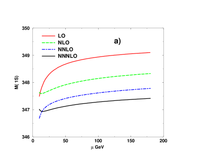
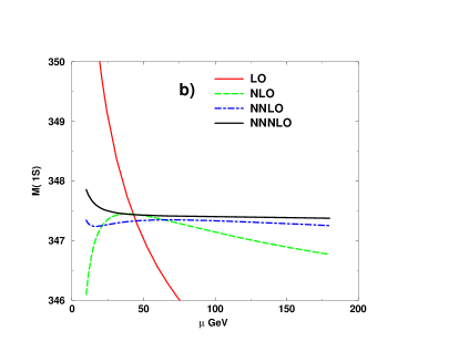
In Figs. 1a) and b),
we show the renormalization scale ()
dependences of the energy level when we use the pole mass and the
mass‡‡‡
The pole- mass relation is known up to 3 loops presently.
The 4-loop correction is replaced by its large- approximation
in our analysis.
,
respectively, to express the energy level.
We used the -expansion [15] to cancel renormalons in the
mass scheme; the relevant formulas are
given in the Appendix.
Fig. 1a) is essentially a reproduction of Fig. 2(b) of [2],
by including the leading order (LO) curve in addition.
As pointed out by [2],
the next-to-next-to-next-to-leading order
(NNNLO) prediction becomes insensitive to the scale variation at
GeV, and that the sum of the and corrections
becomes small around this scale.
Figure 1: The renormalization scale dependences of the energy level of the
vector toponium state
for a) the pole mass scheme and b)
mass scheme, respectively.
The solid curves are the NNNLO results,
dotted, dashed and dot-dashed curves
denote the LO, NLO and NNLO results, respectively.
On the other hand,
in Fig. 1b), we see a good convergence behavior at
–80 GeV.
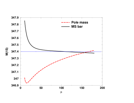
In Fig. 2 the vertical scale is magnified and the scale
dependences of the energy levels at the NNNLO in both mass schemes
are compared.
We find a much better stability of the prediction in the
mass
scheme over a wide region .
From this analysis, we consider the scale –80 GeV
to be an optimal scale choice in the mass scheme.
By varying between 30–160 GeV,
we estimate the theoretical error of the mass to be order
40 MeV at NNNLO if it is extracted from the energy level.
(We obtain an error of about 200 MeV if a similar estimate is applied for
the pole mass.)
In the pole mass scheme, it is natural to choose the renormalization scale
around the Bohr scale,
GeV.
This is because there is only one logarithm
in the energy level,
associated with the renormalization scale ,§§§
At NNNLO, the logarithm associated with the ultrasoft scale
is not accompanied by the renormalization scale .
and because this logarithm is minimized around the Bohr scale.
On the other hand, in the mass scheme,
two types of logarithms
and
are included in the expression for the energy level,¶¶¶
This stems from the fact that one needs to expand the
pole mass and the binding energy in the same coupling constant
in order to achieve the decoupling of infrared degrees of freedom
at each order of the perturbative expansion.
where
is the
renormalization-group invariant mass;
see Eqs. (13), (17) and (18).
Therefore, a natural scale, which minimizes the logarithmic contributions,
lies between the Bohr scale and
the hard scale,
.
This aspect of the renormalization scale, when the leading
renormalon uncertainty is removed,
has been discussed already for the bottomonium energy levels
[16], and a further detailed study of
the scale choice (in the context of the QCD potential)
has been given in [17].
If we replace by ,
the corresponding figures to Figs. 1a,b)
and 2 look very similar;
these were shown in [18].
The main observations in the analysis in the large- approximation
were as follows [12, 18]:
(1) In the pole mass scheme, with any choice of the scale ,
the perturbative series of the energy level does not show
a healthy convergence behavior, hence the level cannot be predicted
with an accuracy better than .
(2) In the mass scheme, one observes a good
convergence of the
perturbative series in the range ,
as well as stability of the prediction in this range.
Both of these observations still hold at the best of our present knowledge.
It is intriguing whether these features will remain valid even
when and the 4-loop relation between
the pole and masses are computed fully in the future.
Let us address how the theoretical error of about 80 MeV
for the top quark pole mass was obtained in Ref. [2].
It is dominated by the uncertainty induced by the error of the input
.
The uncertainty due to the scale dependence was estimated by varying
between 10–30 GeV and an error of 20.5(=41/2) MeV was assigned as
an uncertainty from this source.
Uncertainties from other sources were estimated to be even smaller.
Here, let us concentrate on the error estimate from the scale dependence
and discuss its problem.
The smallness of this error ensures, partly, the smallness of the
total error (80 MeV).
However, if the same estimation method is
applied to the LO and NLO curves in Fig. 1a), we should
infer that the NNLO correction is small, in contradiction
to its true large size.
Thus, apparently there is a danger in relying on this estimation method.
By contrast, our error estimate of the top quark
mass from the scale dependence
does not suffer from the same problem.
The same estimation method works at lower orders,
because the perturbative series in Fig. 1b)
shows a healthy convergence behavior and the
scale dependence decreases as we include more terms around the
relevant scales.
Figure 2: The energy levels of the vector toponium state at NNNLO are plotted
in the pole and schemes.
A horizontal line, GeV, is drawn for
a guide.
At this stage, there seems to be a puzzling point:
on the one hand, the validity
of the large- approximation is known to lead to an
uncertainty of the pole mass;
on the other hand, the small
size of the plus corrections in the range –30 GeV
appears to be incompatible with the renormalon picture.
Let us recall the estimate of the renormalon
uncertainty in the large-
approximation (see e.g. [19]).
Asymptotically the perturbative series of the energy level, if
expressed in the pole mass, behaves as
(4)
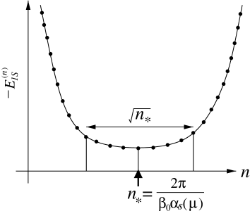
It becomes minimal at .
The size of the term scarcely changes within the range
;
see Fig. 3.∥∥∥
Using the Stirling formula, one may easily find
an approximate position of the minimum of the series.
Then, by expanding around the minimum, one finds an
approximate form
in the range
.
Figure 3: The graph showing schematically the asymptotic behavior of the -th
term of in the large- approximation for .
We may consider the uncertainty of this asymptotic series
as the sum of the terms within this range, since we are not sure
where to truncate the series within this range:
(5)
The -dependence vanishes in this sum, and this leads to the
claimed uncertainty.
This argument shows that when the relevant coupling constant
is small (corresponding scale is large),
is large.
Then each term of the series for
can become considerably smaller than .
According to this argument, the small size of the plus correction
at certain scales does not generally lead to an uncertainty considerably
smaller than .
While an error estimate should necessarily be more or less subjective,
as long as the large- approximation is valid, we should at least bear in mind
how the theoretical uncertainty is estimated in this framework.
Incidentally, based on the large- approximation, the mass extracted from the
energy level has an uncertainty of order
–10 MeV
originating from the next-to-leading order renormalon contribution
[20].
Thus, the above perturbative error of order 40 MeV is still significantly
larger than this contribution.
To conclude, we observe a much more stable prediction of the
toponium energy level when we use the mass instead of the pole
mass.
Considering this situation and the good agreement of the
large- approximation with the presently known
corrections, we consider a theoretical uncertainty of the pole mass
of order –300 MeV to be legitimate.
On the other hand, based on the argument in [12], it is likely
that the top quark mass can be extracted with an accuracy
of order 40 MeV,
once the 4-loop relation between the pole and mass is
calculated.
This number may be compared with the most recent estimate
[21] of the
experimental error (including some systematic errors) of
19 MeV in the determination of the top quark mass,
corresponding to a 3-parameter fit with
an integrated luminosity of 300 fb-1.
Acknowledgement
This work was completed through discussion during the Quarkonium
Working Group Workshop held at CERN in Nov. 2002.
We are grateful to those who participated in the discussion
and in particular to the organizers of this workshop.
Y. K. was supported by the Japan Society for the Promotion of Science.
Appendix
In this appendix we list the formulas we use to convert the
energy level of the quarkonium state from the pole mass scheme to the
mass scheme using the -expansion [15].
The energy of the quarkonium state is given by
(6)
as a function of and
in the pole mass scheme, where is the number of light quark flavors
( for the bottomonium and toponium, respectively).
Mass relation between the pole and masses is given by
(7)
where is the expansion parameter in the -expansion,
, .
The coefficients and are obtained from the 2-loop [22]
and 3-loop [9] mass relations
******
The same relation was obtained numerically before
in [24] in a certain approximation.
,
respectively, by rewriting them in terms of the coupling of the theory with
flavors only. These are given by
(8)
(9)
with .
The third coefficient is not known exactly yet.
In this paper we use its value in the large- approximation
[7]:
(10)
To achieve the renormalon cancellation between and
order by order in the -expansion,
we must use the same coupling constant in the series
expansions of
and .
Therefore, is re-expressed in
terms of as
(11)
using the coefficients of the QCD -function:
(12)
Using Eqs. (7) and (11), we obtain the -expansion
for in terms of ,
(13)
where the coefficients are
functions of which enter via Eq. (11).
The binding energy is given by
(14)
where ,
and are given by
(15)
with
The terms which contain are determined by renormalization-group equation
from lower order constants . The are taken from
[23], is given in Eq. (2).
To obtain the -expansion in the scheme,
we re-express the pole mass in by
and employing the mass relation Eq. (13),
which gives
(17)
with .
Using the -expansions Eqs. (13) and (17),
is rewritten as
(18)
Setting the expansion parameter in the final expression,
the -th order
correction to in the scheme
is given by
.
References
[1]
B. A. Kniehl, A. A. Penin, V. A. Smirnov and M. Steinhauser,
Nucl. Phys.B635, 357 (2002).
[2]
A. A. Penin and M. Steinhauser,
Phys. Lett.B538, 335 (2002).
[3]
N. Brambilla, A. Pineda, J. Soto and A. Vairo,
Phys. Lett.B470, 215 (1999).
[4]
B. A. Kniehl and A. A. Penin,
Nucl. Phys.B577, 197 (2000).
[5]
F. A. Chishtie and V. Elias,
Phys. Lett.B521, 434 (2001).
[6]
A. Hoang, et al.,
Eur. Phys. J. directC3 (2000) 1.
[7]
M. Beneke and V. Braun,
Phys. Lett.B348, 513 (1995).
[8]
M. Beneke,
Phys. Rept.317, 1 (1999).
[9]
K. Melnikov and T. van Ritbergen,
Phys. Lett.B482, 99 (2000).
[10]
D. J. Broadhurst and A. G. Grozin,
Phys. Rev.D52, 4082 (1995).
[11]
C. N. Lovett-Turner and C.J. Maxwell,
Nucl. Phys.B452, 188 (1995).
[12]
Y. Kiyo and Y. Sumino,
Phys. Lett.B496, 83 (2000).
[13]
A. H. Hoang, hep-ph/0008102.
[14]
A. Pineda, JHEP0106, 022 (2001).
[15]
A. Hoang, Z. Ligeti and A. Manohar,
Phys. Rev. Lett.82, 277 (1999);
Phys. Rev.D59, 074017 (1999).
[16]
N. Brambilla, Y. Sumino and A. Vairo,
Phys. Lett.B513, 381 (2001).
[17]
Y. Sumino,
Phys. Rev.D65, 054003 (2002).
[18]
Y. Sumino, hep-ph/0101236; Y. Kiyo, hep-ph/0107209.
[19]
Y. Sumino, hep-ph/0004087.
[20]
U. Aglietti and Z. Ligeti, Phys. Lett.B364, 75 (1995).
[21]
M. Martinez and R. Miquel, hep-ph/0207315.
[22]
N. Gray, D.J. Broadhurst and W. Grafe, K. Schilcher,
Z. Phys.C48, 673 (1990).
[23]
A. Pineda and F. J. Ynduráin,
Phys. Rev.D58, 094022 (1998).
[24]
K.G. Chetyrkin and M. Steinhauser,
Phys. Rev. Lett.83, 4001 (1999);
K.G. Chetyrkin and, M. Steinhauser,
Nucl. Phys.B573, 617 (2000).