1 Introduction

Jet algorithms are tools to reduce information on the hadronic final state resulting from high-energy collisions: instead of analysing a large number of hadrons produced in an event, one could focus on a relatively small number of jets. This helps to concentrate on main features of the underlying physics, the theory of quantum chromodynamics (QCD), as well as allows the reconstruction of heavy particles of the Standard Model.

Jets can be found without jet algorithms. A jet is simply a highly collimated bunch of particles (calorimeter cells, tracks, etc.) that can easily be found after a visual analysis of events. However, to compare observables based on jet momenta with a theory, one needs an objective and a unambiguous jet definition to be used by experimentalists and theorists on an equal footing. In this article, a few most popular definitions of jet algorithms are reviewed.

2 Requirements on jet algorithms

The jet definitions should satisfy the following requirements:

1) Predictions for jets should be infrared and collider safe: i.e. a measured jet cross section should not change if the original parton radiates a soft parton or if it splits into two collinear partons;

2) The decision on which jet algorithm to use has to be based on understanding of the size of high-order QCD corrections. At fixed-order QCD, an observable, $A$, can be expressed by a perturbation series in powers of the strong coupling constant, $A=A_{1}\>\alpha_{s}(\mu_{R})+A_{2}\>\alpha_{s}^{2}(\mu_{R})+B(\mu_{R})$, where $B(\mu_{R})$ denotes missing high-order QCD terms, $\mu_{R}$ is the renormalisation scale used to deal with the ultraviolet divergences ($A$ is independent of $\mu_{R}$). To estimate the contribution from unknown $B(\mu_{R})$, $\mu_{R}$ can be varied within some range. If the renormalisation scale is set to the jet transverse energy, $\mu_{R}=E_{\bot}$, a typical variation presently adopted to estimate the renormalisation scale uncertainty is $0.5E_{\bot}<\mu_{R}<2E_{\bot}$ . An optimal algorithm has to have a small uncertainty associated with such variations. This gives an indication that missing high-order QCD contributions do not change significantly the fixed-order theoretical predictions;

3) Close correspondence with the original parton direction, since the association of jets with hard partons is the basic assumption when the theoretical predictions are compared to the data. This property is essential when simple kinematical considerations are used to reconstruct heavy particles from the invariant mass of two or more jets;

4) An optimal jet definition should have small hadronisation corrections, as well as small hadronisation uncertainties. At HERA, the transverse energies of jets are relatively small, therefore, it is essential to understand these two effects. The hadronisation correction factor, $C$, is evaluated as the ratio $\sigma_{hadrons}^{MC}/\sigma_{partons}^{MC}$, where $\sigma^{MC}$ is the jet cross section obtained using Monte Carlo (MC) models generated for hadrons or partons. For an optimal jet algorithm, $C\sim 1$. Note that such correction factor used to multiply the fixed-order QCD cross sections is not fully justified for every observable: the parton level of MC models is fundamentally non-perturbative because of the QCD cut-off used to deal with divergent integrals, and the number of partons in MC models significantly exceeds the multiplicity of partons for fixed-order calculations. This correction was adopted only in case if: a) a fixed-order QCD calculation and the corresponding parton-level MC prediction well agree ($<5\%$ difference); b) the hadronisation correction is not large ($<20\%$); c) the hadronisation uncertainties are small ($<5\%$). The latter can be found by comparing hadronisation corrections evaluated using the Lund string fragmentation model with the cluster fragmentation models, which are both implemented in MC simulations. Numerous results from HERA indicated that measured jet cross sections better agree with the next-to-leading order (NLO) calculations corrected using the MC hadronisation correction;

5) Suppression of soft processes related to the beam remnants (this will be discussed in more details below);

6) Small experimental uncertainties;

7) Simple to use in experimental analyses and in theoretical calculations. Note that the same jet algorithm has to be uniquely defined for experimental and theoretical calculation inputs, without any additional modification.

First, we will discuss jet algorithms for $e^{+}e^{-}$ collisions when there are no spectator jets (see [2] for more details). In this respect, $e^{+}e^{-}$ jet algorithms are simpler than those for hadron collisions.

3 Clustering algorithms for $e^{+}e^{-}$

The $e^{+}e^{-}$ collisions occur in the centre-of-mass frame, which coincides with the laboratory frame. Thus, it is desirable to find a two-particle distance measure which is invariant under the rotations. In this case, a good choice is the energy, $E_{i}$, and the polar angle, $\theta_{i}$, of the $i$th particle. The distance measure for two particles, $d_{ij}^{2}$, can be defined as $d_{ij}^{2}=2E_{i}E_{j}(1-\cos\theta_{ij})$, where $\theta_{ij}$ is the opening angle between two particles. More often, $y_{ij}=d_{ij}^{2}/E_{vis}^{2}$, with $E_{vis}$ being the visible event energy, is used. This gives some cancelation of errors between numerator and denominator. Note that when masses of hadrons (partons) are set to zero, the variable $d_{ij}$ coincides with the invariant mass of two particles. The reason for this choice is obvious: particles tend to cluster closer in invariant mass in the region of small momenta.

This distance measure was used by the JADE collaboration [1] to define jets in the following way: The algorithm starts with the initial list of particles. The two particles are merged into one, provided that their distance $y_{ij}$ is smaller than the desired minimum separation, $y_{cut}$. This procedure is repeated until all pairs of clusters have separations above $y_{cut}$.

It has soon been realized that the fixed-order QCD corrections are sizeable for the JADE algorithm. The explanation is following: soft gluons, which are copiously radiated far apart, may have a small distance measure ($E_{i}E_{j}\sim 0$). This leads to a “phantom” jets which do not reflect the hardness of jets. It is likely that this feature has a direct impact on the reconstruction of heavy particles decaying into jets, since the use of JADE algorithm for the reconstruction of $W$ bosons [2] and top quarks [3] in $e^{+}e^{-}$ is less successful than for other algorithms.

The solution was found by replacing the JADE distance measure by the following construction: $d_{ij}^{2}=2\cdot\min(E_{i}^{2},E_{j}^{2})(1-\cos\theta_{ij})$, which corresponds to the square of the transverse energy, $E_{\bot}^{2}$, of the lower-energy particle with respect to a reference direction given by the higher-energy parton, since for small angles $d_{ij}^{2}\sim 2\cdot\min(E_{i}^{2},E_{j}^{2})\cdot\sin\theta_{ij}^{2}=E_{\bot}^{2}$. The jet-clustering based on this distance measure is called the Durham or the $k_{\bot}$ algorithm [4]. In this algorithm, the soft gluons are combined first with the nearby high-order quark, thus the $k_{\bot}$ algorithm avoids the problem of unnatural assignments of particles to jets.

For $e^{+}e^{-}$, other algorithms, such as LUCLUS, GENEVA, Angular-ordering Durham, CAMBRIDGE and DICLUS are also often used (see [2] for details).

4 Jet algorithms for $ep$ and $p\bar{p}$ collisions.

4.1 Differences between $e^{+}e^{-}$ and hadron collisions

For more complicated colliding particles, the initial-state system is not at rest and the laboratory frame is less often used. The hadronic centre-of-mass frame and the Breit frame (for $ep$ collisions in DIS regime) are the most natural choice.

There are a few reasons why the jet algorithms used in $e^{+}e^{-}$ cannot be applied directly to collisions with more complicated initial state: a) In $e^{+}e^{-}$, the entire event arises from the collision, thus one usually measures the exclusive jet cross sections, i.e. when all produced particles are grouped into jets and the cross sections describe the production of exactly $N$ number of jets and nothing else. In hadron-hadron collisions, it is more convenient to analyse inclusive high $E_{\bot}$ cross sections, i.e. when some number of jets plus any number of unobserved jets/particles are reconstructed. In this case, only a small fraction of the final-state hadrons is associated with the large momentum transfer and hard scattering; b) The previous comment is easy to understand noting that the beam-remnant jet has huge energies, but it does not undergone a hard scattering. Thus, the algorithm for hadron collisions should avoid clustering particles with small transverse momenta with respect to the beam direction, reducing contributions due to the “underlying event”; c) Finally, in contrast to $e^{+}e^{-}$ events, where the rotation invariance is important, for the hadron collisions one wants to emphasize the invariance under the boost along the beam axis, as the partonic system is boosted along the direction of colliding hadrons. In this case, the separation between particles can be defined in terms of the transverse energy, $E_{\bot}$, azimuthal angle, $\phi$, and the pseudorapidity difference, $\Delta\eta$ ($\eta=-\ln(\tan(\theta/2))$).

4.2 The cone algorithm

The cone algorithm has been used for a long time to define jets at hadron colliders [5]. Every calorimeter cell with energy above $E_{0}$ is considered as a seed cell (for the D0 choice, $E_{0}=1$ GeV). Then, a jet is defined by summing all cells within the cone $R_{cone}=\sqrt{(\eta_{i}-\eta_{seed})^{2}+(\phi_{i}-\phi_{seed})^{2}}$, which is taken to be 0.7. The jet directions can be found as $\eta_{jet}=\sum_{i\in cone}E_{\bot i}\eta_{i}/E_{\bot{jet}}$, $\phi_{jet}=\sum_{i\in cone}E_{\bot i}\phi_{i}/E_{\bot{jet}}$, $E_{\bot{jet}}=\sum_{i\in cone}E_{\bot i}$. If the jet direction does not coincide with the seed cell, the procedure is reiterated, replacing the seed cell by the current jet direction, until a stable jet configuration is obtained. After this, jets which are duplicated or below some energy thresholds have to be thrown away. Since there is no attempt to combine hadrons into the remnant jets, this algorithm is used to reconstruct inclusive jet cross sections. Some jets could be overlapping. To deal with this problem, the following procedure was adopted: any jet that has more than $50\%$ of its energy in common with a higher-energy jet is merged with that jet (according to the D0 definition). Any jet that has less than $50\%$ of its energy in common with a higher-energy jet is split from that jet. In case of the CDF and ZEUS algorithms, the energy merging/splitting threshold is $75\%$. Note that after the merging/splitting procedure, the size of the cone jets is not always equal to $R_{cone}=0.7$.

As it is clear from the above consideration, the cone algorithm is not precisely defined, and there are many details which can affect the theoretical results obtained using the cone-jet definition. Thus, anyone calculating theoretical predictions must know the very precise way of how this algorithm was implemented. In this respect, clustering algorithms to be discussed below do not suffer from the ambiguities characteristic for the cone algorithm.

4.3 The modified JADE algorithm

This algorithm was one of the first algorithms used at HERA to reconstruct jets and to determine the $\alpha_{s}$ values from the jet rates. Since the $ep$ hadronic final state is not as complicated as for hadron-hadron collisions, one could slightly modify the JADE $e^{+}e^{-}$ algorithm by taking into account the new feature - the proton remnant jet, but ignoring the requirement that the variables should be invariant under the boost [6]: In order to cluster soft partons into the remnant jet, a pseudo-particle which carries the missing longitudinal momentum in the forward region was inserted. After the clustering, one ends up with $N+1$ jets (where ”+1” denotes the proton-remnant jet). If no any experimental cuts on the jet kinematics are applied, this algorithm can be used to measure the exclusive jet cross sections.

4.4 The $k_{\bot}$ algorithm

It is clear that the modified JADE algorithm has the same disadvantages as the standard JADE algorithm for $e^{+}e^{-}$ annihilations: soft gluons can be combined into phantom jets even if the gluons are far apart. Thus, the $k_{\bot}$ scheme should be used as a basis for the exclusive jet definitions for hadron collisions. In contrast to the JADE algorithm, however, it was proposed [7] to use another method to deal with the proton remnant jets in $ep$ collisions: one can define the distance from the proton direction as $y_{k}=2\cdot(1-\cos\theta_{k})E_{k}^{2}/E_{\bot}^{2}$. Here, $E_{\bot}$ stands a hard scattering scale and $\theta_{k}$ is the angle of a particle with respect to the beam direction. Analogously, $y_{kl}=2\cdot(1-\cos\theta_{kl})\cdot\min(E_{k}^{2},\,E_{l}^{2})/E_{\bot}^{2}$ can be defined for every particle pair. Then, the smallest value among $\{y_{k},y_{kl}\}$ should be taken. If $y_{kl}$ is the smallest and $y_{kl}<1$, two particles are combined into a single cluster, $p_{kl}=p_{k}+p_{l}$. If $y_{k}$ is the smallest and $y_{k}<1$, the particle is included into the beam jet. This procedure is repeated until all clusters have $y_{k},\,y_{kl}>1$. The final results are the remnant jet and some number of hard jets. This method was proposed for the Breit frame of DIS.

This algorithm can also be used for $p\bar{p}$ collisions if one adds an additional distance measure for the second proton directions [7].

4.5 The longitudinally invariant $k_{\bot}$ algorithm

The two previous clustering algorithms were designed as close as possible to the clustering algorithms used in $e^{+}e^{-}$, i. e. they focus on the exclusive jet definitions. However, it is possible to focus on the inclusive jet definition from the very beginning, by modifying the jet clustering procedure. In addition, one can redefine the distance measure keeping similarity with the cone algorithm and using the longitudinally invariant variables for the distance measure. Such an algorithm can be constructed in the following way [8]: For each particle and particle pair, one should define $d_{i}=E_{\bot i}^{2}$ and $d_{ij}=R^{-2}\min(E_{\bot i}^{2},E_{\bot j}^{2})[(\eta_{i}-\eta_{j})^{2}+(\phi_{i}-\phi_{j})^{2}]$, respectively ($R$ is a free parameter). Then, one finds the smallest of all the $d_{i}$ and $d_{ij}$. If $d_{ij}$ is the smallest, particles are merged into a new cluster. If the smallest is $d_{i}$, this particle should be removed from the list. This procedure continues until there are no more particles/clusters, and as it proceeds, it produces a list of jets with successively larger values of $d_{i}=E_{\bot i}^{2}$. After some cuts on the jet transverse energy, only a few jets with high $E_{\bot}$ can be used for comparisons with theory. According to the perturbative calculations [8], if $R\simeq 1.35R_{cone}\simeq 1$, the inclusive jet cross sections obtained with this algorithm are very close to those reconstructed using the cone algorithm.

Such a modification of the exclusive $k_{\bot}$ algorithm has also been proposed in [9], noting that the original $k_{\bot}$ algorithm is longitudinal invariant only in the small-angle limit. However, it admits a longitudinal-boost-invariant extrapolation to large angles if the distance measure is defined as $d_{ij}=\min(E_{\bot i}^{2},E_{\bot j}^{2})[(\eta_{i}-\eta_{j})^{2}+(\phi_{i}-\phi_{j})^{2}]$.

5 Differences between algorithms

5.1 Exclusive algorithms

The major disadvantage of the JADE algorithm is in its significant recombination scheme dependence; widely separated soft partons can be clustered, even though these partons do not form a pencil-like jet. As a consequence, this leads to large high-order QCD corrections (for example, see [10]).

5.2 Inclusive jet algorithms

The cone and the longitudinally invariant inclusive $k_{\bot}$ algorithm allow the reconstruction of the inclusive jet cross sections. Such cross sections are less informative than the exclusive ones reconstructed with exclusive algorithms which force all particles into a given number of jets. Nevertheless, the inclusive jets are sufficient for studies of hard QCD, since jets with high $E_{\bot}$ reflect large momentum transfer. In addition, the high-$E_{\bot}$ jets have the hadronisation and detector corrections significantly smaller than for jets with low $E_{\bot}$. The latter are less reliably reconstructed and might be attributed the hadron debris. Exclusive jet algorithms can also produce the inclusive cross sections by ignoring jets with low $E_{\bot}$.

The exclusive $k_{\bot}$ algorithm in the small-angle limit is identical to the longitudinally invariant $k_{\bot}$ algorithm: the difference appears for large angles when the longitudinally invariant algorithm is somewhat closely related to the cone algorithm. This simplifies the comparisons with the results obtained using the cone algorithm. The major differences between the longitudinally invariant $k_{\bot}$ algorithm and the cone algorithm are:

1) The longitudinally invariant $k_{\bot}$ algorithm (as any other algorithm based on the recombination procedure) never assigns a particle to more than one jet, which is not the case for the cone algorithm; for the latter, an arbitrary procedure is necessary to deal with this problem.

2) The distribution of transverse energy within jets is different. The cone algorithm has well defined smooth boundaries irrespective of the energy distribution of the hadronic activity inside the jet. This typically leads to more transverse energy near the cone edges than in case of the longitudinally invariant algorithm. The latter can have rather complicated boundaries depending on the energy flow within jet (see Fig. 1). As a direct consequence, the resolution on the reconstruction of the invariant masses of heavy particles from jets is better when the cluster $k_{\bot}$ algorithm is used [12].

3) The cone algorithm is not infrared safe [13] at the next-to-next-leading-order QCD for $p\bar{p}$ process, when jets begin to develop internal structure. As a reflection of this, the cone algorithm has large renormalisation scale uncertainties already at next-to-leading order QCD calculations for dijet cross sections in DIS (in fact, the cross sections determined with the cone algorithm are negative if the laboratory frame is used, indicating very large renormalisation scale uncertainties). A finite calorimeter cell size and minimum energy $E_{0}$ used to define the seeds render finite cone-jet cross sections. The seeds were always considered by experimentalist as an insignificant detail in the jet founding, since the seeds only help to find stable jet directions. However, the energies and the size of the seeds are very important for high-order QCD calculations, since the jet cross sections depend logarithmically on the energy threshold above which calorimeter cells are considered as seed cells in the overlap regions of two cone jets.

In contrast to the cone algorithm, the $k_{\bot}$ algorithm is infrared and collinear safe to all orders of QCD calculations, and it does not require the arbitrary splitting/merging procedure.

6 Experimental situation

The standard jet algorithm used by the D0 and CDF Collaborations is based on the cone definition. Recently, for the first time, the D0 used the longitudinally invariant $k_{\bot}$ algorithm to measure inclusive jet cross sections [15]. The obtained results indicated that the experimental cross sections are rather different to those reconstructed with the cone algorithm, although the theoretical predictions are very similar for both algorithms. This might be attributed to different hadronisation corrections and/or to a contribution from spectator partons. The CDF and D0 plan to use the $k_{\bot}$ algorithm in Run II.

At HERA, the cone algorithm (PUCELL, a rather similar to the CDF definition) was frequently used in the past. At present, almost all jet physics at HERA is based on the $k_{\bot}$ algorithm (see Fig. 2). This algorithm significantly simplifies the data analysis, leads to small hadronisation corrections $(<10-20\%)$ and hadronisation uncertainties $(<3\%)$, as well as to small renormalisation scale dependence $(<10-20\%)$. Experimental uncertainties are usually smaller than the theoretical, and are typically below $3-5\%$ for the jet transverse energies $E_{\bot}\sim 15-30$ GeV. This ultimately allows high precision measurements. As an example, a recent determination of the strong coupling constant from the inclusive jets at HERA [16] has by a factor three less theoretical uncertainties than a similar measurement based on the cone algorithm [17]. Whether this can be attributed to the use of the $k_{\bot}$ algorithm, or due to indisputable more complicated initial state of colliding particles at TEVATRON is not yet clear and requires a careful examination.

In conclusion, it should be stressed that future developments of the jet algorithms should mainly depend on understanding of multiple-gluon emissions and high-order QCD contributions. The jet-algorithm definitions should not be motivated by efforts to minimize experimental-related effects, which are nowadays significantly smaller than the renormalisation-scale dependence. Note that future developments might be rather unexpected; first steps beyond the jet clustering algorithms have already been undertaking [18], focusing on instabilities of the jet clustering algorithms and indisputable ambiguity of their definitions.

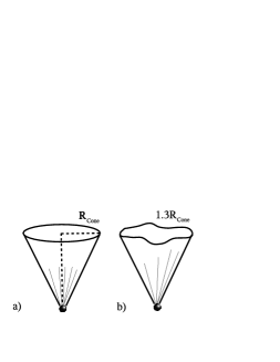
Figure 1: Topologies of jet shape for the cone (a) and for the longitudinally invariant $k_{\bot}$ (b) algorithm.

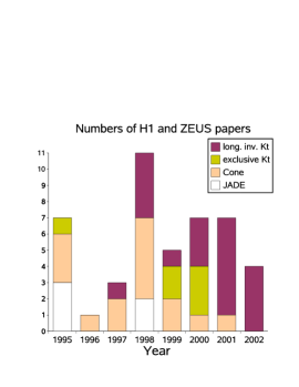
Figure 2: The numbers of H1 and ZEUS published papers based on jet algorithms. Note that year of the articles does not always coincide with year of publication.

References

- [1] JADE Collaboration, W. Bartel et al., Z. Phys. C 33, 23 (1986); S. Bethke, Habilitation thesis, LBL 50-208 (1987)
- [2] S. Moretti, L. Lönnblad, T. Sjöstrand, JHEP 9808 001,(1998)
- [3] S. Chekanov, hep-ph/0206264, Eur. Phys. J C (in press)
- [4] S. Catani et al., Phys. Lett. B 269, 432 (1991)
- [5] J. Huth et al., in Proc. of Research Directions for the Decade, Snowmass 1990, edited by E.L.Berger (World Scientific, Singapore, 1992)
- [6] T. Brodkorb, J.G. Körner, E. Mirkes, G.A. Schuler, Z. Phys. C 44, 415 (1989)
- [7] S. Catani, Yu.L. Dokshitzer and B.R. Webber, Phys. Lett. B 285, 291 (1992)
- [8] S.D. Ellis and D.E.Soper, Phys. Rev. B 48, 3160 (1993)
- [9] S. Catani et al., Nucl. Phys. B 406, 187 (1993)
- [10] E. Mirkes and D. Zeppenfeld, Proc. of 5th International Workshop, ed. by J.Repond and D.Krakauer (Chicago, April, 1997), p.659
- [11] M.H. Seymour, Z. Phys. C 62, 127 (1994)
- [12] M.H. Seymour, Nucl. Phys. B 421, 545 (1994)
-
[13]
W.T. Giele and W.B. Kilgore, Phys. Rev. D 55, 7183 (1997);
M.H. Seymour, Nucl. Phys. B 513, 269 (1998) - [14] B. Pötter and M.H. Seymour, J. Phys. G 25, 1473 (1999)
- [15] D0 Coll., V.M.Abazov, Phys. Lett. B 525 211, (2002)
- [16] ZEUS Coll., S. Chekanov et al, DESY-02-112, Phys. Lett. B (in press)
- [17] CDF Coll., T. Affolder, FERMILAB-PUB-01-246-E, Phys. Rev. Lett. (in press)
- [18] F.V. Tkachov, Int. J. Mod. Phys. A 12, 5411 (1997); Int. J. Mod. Phys. A 17, 2783 (2002)