TUM-HEP-464/02

MPI-PhT/2002-69

Synergies between the first-generation JHF-SK and NuMI superbeam experiments^∗

P. Huber,  M. Lindner, and  W. Winter 

^,,Institut für theoretische Physik, Physik–Department, Technische Universität München,

James–Franck–Strasse, D–85748 Garching, Germany

Max-Planck-Institut für Physik, Postfach 401212, D–80805 München, Germany

Abstract

We discuss synergies in the combination of the first-generation JHF to Super-Kamiokande and NuMI off-axis superbeam experiments. With synergies we mean effects which go beyond simply adding the statistics of the two experiments. As a first important result, we do not observe interesting synergy effects in the combination of the two experiments as they are planned right now. However, we find that with minor modifications, such as a different NuMI baseline or a partial antineutrino running, one could do much richer physics with both experiments combined. Specifically, we demonstrate that one could, depending on the value of the solar mass squared difference, either measure the sign of the atmospheric mass squared difference or CP violation already with the initial stage experiments. Our main results are presented in a way that can be easily interpreted in terms of the forthcoming KamLAND result.

1 Introduction

There exists now very strong evidence for atmospheric neutrino oscillations, since there is some sensitivity to the characteristic $L/E$ dependence of oscillations [1]. Solar neutrinos also undergo flavor transitions [2, 3] solving the long standing solar neutrino problem, even though the $L/E$ dependence of oscillations is in this case not yet established. Oscillations are, however, by far the most plausible explanation and global fits to all available data clearly favor the so-called LMA solution for the mass splittings and mixings [4, 5, 6, 7]. The CHOOZ reactor experiment [8] moreover currently provides the most stringent upper bound for the sub-leading $U_{e3}$ element of the neutrino mixing matrix. The atmospheric ${\Delta m^{2}_{31}}$-value defines via ${\Delta m^{2}_{31}}L/E_{\nu}=\pi/2$ the position of the first oscillation maximum $L$ as function of the energy $E_{\nu}$. This leads for typical energies of $E_{\nu}\sim 1-100\,\mathrm{GeV}$ to long-baseline (LBL) experiments, such as the ongoing K2K experiment [9], the MINOS [10] and CNGS [11] experiments just being constructed, and planned “superbeam” [12, 13, 14, 15, 16, 17, 18, 19, 20, 21, 22] or “neutrino factory” experiments [23, 24, 25, 26, 27, 28, 29, 30, 31, 32, 33, 34, 35, 36]. The solar ${\Delta m^{2}_{21}}$ is, for the favored LMA solution, about two orders of magnitude smaller than the atmospheric ${\Delta m^{2}_{31}}$, resulting in much longer oscillations lengths for similar energies. The solar oscillations will thus not fully develop in LBL experiments, but sub-leading effects play an important role in precision experiments. Together with matter effects [37, 38, 39, 40], interesting physics opportunities are, in principle, opened, such as the extraction of the sign of ${\Delta m^{2}_{31}}$ or the detection of CP violation in the lepton sector. However, correlations and intrinsic degeneracies [15, 30, 41] in the neutrino oscillation formulas turn out to make the analysis of LBL experiments very complicated. Fortunately, the potential to at least partially resolve those by the combination of different experiments has been discovered [42, 43, 44, 19, 45, 46].

Experimental LBL studies often assume that experiments with different levels of sensitivity are built successively after each other. For example, a frequent scenario is that a superbeam experiment (especially JHF) is followed by a neutrino factory with one or several baselines. However, there exist competing superbeam proposals, such as for the the JHF to Super-Kamiokande (JHF-SK) [14] and the NuMI [22] projects, which are some of the most promising alternatives for the next generation LBL experiments. Both are, in their current form, optimized for themselves for a similar value of $L/E$ corresponding to the current atmospheric best-fit value of $\Delta m_{31}^{2}=3.0\cdot 10^{-3}\,\mathrm{eV}^{2}$. Building both experiments together would lead to improved measurements because of the luminosity increase, but one may ask if there are synergies in this combination, i.e., complementary effects which not only come from the better statistics of both experiments combined. In this paper, we study, from a purely scientific point of view, the question if the two experiments are more than the sum of their parts, or if it would (in principle) be better to combine resources into one larger project. We are especially interested in comparable versions of the initial stage options with running times of five years each, which means that the first results could be obtained within this decade. Thus, in comparison to Ref. [45], we do not assume high-luminosity upgrades of both superbeam experiments, which leads to somewhat different effects in the analysis because we are operating in the (low) statistics dominated regime. In addition, we include in our analysis systematics, multi-parameter correlations, external input, such as from the KamLAND experiment, degeneracies, and the matter density uncertainty.

In Section 2, we will define synergy effects in more detail. Next, we will address in Section 3 (together with some more details in the Appendix) the experiments and their simulation, as well as we will show in Section 4 the relevant analytical structure of the neutrino oscillation framework. As the first part of the results, we demonstrate in Section 5 that there are no real synergies between the experiments as they are planned right now. As the second part, we will investigate in Section 6 alternative option to improve the physical potential of the combined experiments. Eventually, we will summarize in Section 7 the best of those alternative options together with a possible strategy to proceed.

2 How to define synergy effects

We define the extra gain in the combination of the experiments beyond a simple addition of statistics as the synergy among two or more experiments. A reasonable definition of synergy must therefore subtract, in a suitable way, the increase of statistics of otherwise more or less equivalent experiments. In this section, we demonstrate that one possibility to evaluate the synergy effects is to compare the output of the combination of experiments, i.e., the sensitivity or precision of certain observables, to a reference experiment with the corresponding scaling of the integrated luminosity.

A LBL experiment is, beyond statistics, influenced by several different sources of errors, such as systematical errors, multi-parameter correlations, intrinsic degeneracies in the neutrino oscillation formulas, the matter density uncertainty, and external input on the solar oscillation parameters. These errors can be reduced by combining different experiments, such as it has been demonstrated for the intrinsic degeneracies in Refs. [42, 43, 44, 19, 45, 46]. In this spirit we will discuss how the synergies of different LBL experiments can be quantified as effects which go beyond the increase in integrated luminosity.

Such a discussion makes only sense for similar experiments of similar capabilities. In this paper, we use two proposed superbeam experiments with equal running times and similar levels of sophistication, i.e., the JHF-SK and NuMI setups. It is obvious that the combination of two experiments with similar technology but sizes different by orders of magnitude will be dominated by the the bigger experiment. It is also obvious that the combined fit of more than one experiment will, for comparable setups, be much better than the fit of each of the individual experiments. However, the improvement may come from better statistics only or from a combination of the better statistics with other effects, such as complementary systematics, correlations, and degeneracies. We are especially interested in the latter part, since instead of building a second experiment, one could also run the first one twice as long or built a larger detector. The synergy is thus related to the improvement of the measurement coming from complementary information of the different experiments.

It should be clear that we need a method to subtract the luminosity increase coming from the combination of different experiments is needed, in order to compare the results of combined experiments to the ones of the individual experiments. Since we assume equal running times of the individual experiments, we can multiply the individual luminosities (running times or target masses) by the number of experiments $N$ to be combined, and compare the obtained new experiments with the combination of all experiments operated with their original luminosities. This method can be easily understood for the two experiments in this paper: we simulate JHF-SK or NuMI with twice their original luminosity, i.e., running time or target mass, and compare it to the combination of the two experiments in which the experiments are simulated with their original (single) luminosity. We refer to the experiments at double luminosities further on with JHF-SK_2L and NuMI_2L. The difference between the results of the combined experiments and the results of an individual experiment at double luminosity then tells us if there is a real synergy effect, which can not only be explained by the luminosity increase. From the point of view of the precision of the measurement, it tells us if it were better to run one experiment twice as long as it was originally intended (or build a twice as big detector) or if it were better to build a second experiment instead. To compare, we show the curves for JHF-SK_2L or NuMI_2L at double luminosity instead of (or in addition to) JHF-SK and NuMI at single luminosity.

3 The experiments and their simulation

The two experiments considered in this study are the JHF to Super-Kamiokande [14] and the NuMI [22] projects using the beams in off-axis configurations, referred to as “JHF-SK” and “NuMI”. Both projects will use the ${\nu_{\mu}\rightarrow\nu_{e}}$ appearance channel in order to measure or improve the limits on $\sin^{2}2\theta_{13}$. Neutrino beams produced by meson decays always contain an irreducible fraction of $\nu_{e}$, as well as they have a large high energy tail. Therefore, both experiments will exploit the off-axis technology, i.e., building the detector slightly off the axis described by the decay pipe, to make the spectrum much narrower in energy and to suppress the $\nu_{e}$ component [48]. An off-axis beam thus reaches the low background levels necessary for a good sensitivity to the ${\nu_{\mu}\rightarrow\nu_{e}}$ appearance signal. Both experiments are planned to be operated at nearly the same $L/E$, which is optimized for the first maximum of the atmospheric oscillation pattern for a value of ${\Delta m^{2}_{31}}=3.0\cdot 10^{-3}\,\mathrm{eV}^{2}$.

	JHF-SK	NuMI
Beam
Baseline	$295\,\mathrm{km}$	$712\,\mathrm{km}$
Target Power	$0.77\,\mathrm{MW}$	$0.4\,\mathrm{MW}$
Off-axis angle	$2^{\circ}$	$0.72^{\circ}$
Mean energy	$0.76\,\mathrm{GeV}$	$2.22\,\mathrm{GeV}$
Mean $L/E$	$385\,\mathrm{km}\,\mathrm{GeV}^{-1}$	$320\,\mathrm{km}\,\mathrm{GeV}^{-1}$
Detector
Technology	Water Cherenkov	Low-Z calorimeter
Fiducial mass	$22.5\,\mathrm{kt}$	$17\,\mathrm{kt}$
Running period	5 years	5 years

Table 1: The two beams and detectors as given in Refs. [14, 22]

Because of the different energies of the two beams, different detector technologies are used. For the JHF beam, Super-Kamiokande, a water Cherenkov detector with a fiducial mass of $22.5\,\mathrm{kt}$, is used. The Super-Kamiokande detector has an excellent electron muon separation and NC (neutral current) rejection. For the NuMI beam, a low-Z calorimeter with a fiducial mass of $17\,\mathrm{kt}$ is planned, because the hadronic fraction of the energy deposition is much larger at those energies. In spite of the very different detector technologies, their performances in terms of background levels and efficiencies are rather similar. The actual numbers for these quantities and the respective energy resolution of the detectors can be found in the Appendix. For a quick comparison, we give in Table 2 the signal and background rates for the two experiments at the CHOOZ bound of $\sin^{2}2\theta_{13}=0.1$.

	JHF-SK	NuMI
Signal	137.8	132.0
Background	22.6	19.0

Table 2: The signal and background rates for the JHF-SK and NuMI experiments at $\sin^{2}2\theta_{13}=0.1$, $\sin^{2}2\theta_{12}=0.8$, $\sin^{2}2\theta_{23}=1$, ${\Delta m^{2}_{31}}=3.0\cdot 10^{-3}\,\mathrm{eV}^{2}$, ${\Delta m^{2}_{21}}=5.0\cdot 10^{-5}\,\mathrm{eV}^{2}$ and $\delta_{\mathrm{CP}}=0$ for five years of neutrino running.

The event numbers are similar, but there are subtle differences in their origin and composition. For example, the fraction of QE (quasi-elastic scattering) events is much larger in the JHF-SK sample, whereas the matter effect is much more present in the NuMI sample. In fact, the matter effect strongly enhances the NuMI signal compared to the JHF-SK signal.

For the calculation of the event rates, we follow the procedure described in detail in Appendix A of Ref. [47]. Basically we fold the fluxes as given in Ref. [14, 49] with the cross sections from Ref. [50], while we use the energy resolution functions as defined in Ref. [47] in order to obtain realistic detector simulations. The probability calculations are performed numerically within a full three flavor scheme, taking into account the matter effects in a constant average density profile. The parameterizations of the energy resolution functions and the efficiencies can be found in the Appendix.

The evaluation of the precision or the sensitivity for any quantity of interest requires a statistical analysis of the simulated data because of the low rate counts. Thus, we employ a $\chi^{2}$-based method which is described in Appendix C of Ref. [47]. We essentially fit all existing information simultaneously, which especially means that information from the appearance and disappearance channels is used at the same time in order to extract as much information as possible. Beyond the statistical errors, we summarized in Section 3 of Ref. [47] that there are other additional sources of errors limiting the precision of the measurement. First, we take into account systematical errors (cf. the Appendix), since especially background uncertainties can limit the precision of superbeam experiments with good statistics. Second, we employ the full multi-parameter correlations among the six oscillation parameters plus the matter density, which sizably increase the error bars. Third, we use external information on the solar parameters and the matter density. In the appearance probabilities, the solar parameters enter, up to the second order, only via the product ${\Delta m^{2}_{21}}\cdot\sin 2\theta_{12}$. Therefore, we include for this product an error of $15\%$ which is supposed to come from the KamLAND experiment [51, 52]. For the average matter density $\rho=2.8\,\mathrm{g}\,\mathrm{cm}^{-3}$, we assume a precision of $5\%$ [53]. This value contains the contribution of a possible large error on the first Fourier coefficient of the profile as described in Refs. [54, 55] and is shown to be a rather conservative estimate for more complicated models [56, 57, 58, 59]. The other oscillation parameters, such as the atmospheric parameters, are measured by the appearance or disappearance rates of the experiments itself such that no external input is needed. Finally, we include in our analysis very carefully the three degeneracies present in neutrino oscillations (see next section). We essentially follow the methods in Ref. [47], which will be described later in greater detail.

4 The neutrino oscillation framework

Our results are based on a complete numerical analysis including matter effects. It is nevertheless useful to have a qualitative understanding of the relevant effects. We assume standard three neutrino mixing and parameterize the leptonic mixing matrix $U$ in the same way as the quark mixing matrix [60]. In order to obtain intuitively manageable expressions, one can expand the general oscillation probabilities in powers of the small mass hierarchy parameter $\alpha\equiv{\Delta m^{2}_{21}}/{\Delta m^{2}_{31}}$ and the small mixing angle $\sin 2\theta_{13}$. Though one can also include matter effects in such an approximation, we will, for the sake of simplicity, use here the formulas in vacuum [31, 61, 26]. Note that the expansion in $\sin 2\theta_{13}$ is always good, since this mixing angle is known to be small. However, the expansion in $\alpha$ is only a good approximation as long as the oscillation governed by the solar mass squared difference is small compared to the leading atmospheric oscillation, i.e., $\alpha\,\Delta\lesssim 1$. It turns out that the expansion in $\alpha$ can therefore be used for baselines below $L\ll 8000\,\mathrm{km}\left(E_{\nu}/\,\mathrm{GeV}\right)\left(10^{-4}\,\mathrm{eV}^{2}/{\Delta m^{2}_{21}}\right)$, which is fulfilled for the experiments under consideration if $\Delta m_{21}^{2}$ is small enough. The leading terms in small quantities are for the vacuum appearance probabilities and disappearance probabilities

$$P_{e\mu} \simeq \sin^{2}2\theta_{13}\,\sin^{2}\theta_{23}\sin^{2}{\Delta}$$ (1)

$$\mp \alpha\;\sin 2\theta_{13}\,\sin\delta_{\mathrm{CP}}\,\cos\theta_{13}\sin 2\theta_{12}\sin 2\theta_{23}\sin^{3}{\Delta}$$

$$- \alpha\;\sin 2\theta_{13}\,\cos\delta_{\mathrm{CP}}\,\cos\theta_{13}\sin 2\theta_{12}\sin 2\theta_{23}\cos{\Delta}\sin^{2}{\Delta}$$

$$+ \alpha^{2}\,\cos^{2}\theta_{23}\sin^{2}2\theta_{12}\sin^{2}{\Delta},$$

$$P_{\mu\mu} \simeq 1-\cos^{2}\theta_{13}\sin^{2}2\theta_{23}\sin^{2}{\Delta}$$ (2)

$$+ 2\alpha\cos^{2}\theta_{13}\cos^{2}\theta_{12}\sin^{2}2\theta_{23}{\Delta}\cos{\Delta}.$$

The actual numerical values of $\alpha$ and $\sin^{2}2\theta_{13}$ give each term in Equations (1) and (2) a relative weight. In the LMA case, we have $\alpha\simeq 10^{-2\pm 1}$. Thus, in terms of $\sin^{2}2\theta_{13}$, the first term in Equation (1) is dominating for $\sin^{2}2\theta_{13}\simeq 0.1$ close to the CHOOZ bound. For smaller values of $\sin^{2}2\theta_{13}$ all terms are contributing equally, until for very small values $\sin 2\theta_{13}\ll\alpha$ the $\alpha^{2}$ term is dominating. For long baselines, such as the proposed NuMI baselines, the above formulas have to be corrected by matter effects [37, 38, 39, 40]. Analytical expressions for the transition probabilities in matter can be found in Refs. [25, 61, 26]. It turns out that especially the first term in Equation (1) is strongly modified by resonant conversion in matter.

Another important issue for three-flavor neutrino oscillation formulas are parameter degeneracies, implying that one or more degenerate parameter solutions may fit the reference rate vector at the chosen confidence level. In total, there are three independent two-fold degeneracies, i.e., an overall “eight–fold” degeneracy [41]:

The $\mathrm{sgn}(\Delta m_{31}^{2})$ degeneracy:

A degenerate solution for the opposite sign of $\Delta m_{31}$ [15] can often be found close to the $\delta_{\mathrm{CP}}$-$\theta_{13}$-plane (other parameters fixed), but does not necessarily have to lie exactly in the plane. This degeneracy can, in principle, be lifted by matter effects. It is the most important degeneracy in this study.

The $(\delta_{\mathrm{CP}},\theta_{13})$ ambiguity:

The $(\delta_{\mathrm{CP}},\theta_{13})$ ambiguity, which allows a degenerate solution in the $\delta_{\mathrm{CP}}$-$\theta_{13}$-plane for the same sign of $\Delta m_{31}^{2}$, is, in principle, always present [30]. However, it depends on the combination of the oscillation channels if it appears as disconnected solution or not. It is, for our study, only relevant as disconnected solution if neutrino and antineutrino channels are used simultaneously. Otherwise it appears only as one very large solution which closely follows the iso-event rate curve in the $\delta_{\mathrm{CP}}$-$\theta_{13}$-plane. The position of the second solution can be found almost exactly in the $\delta_{\mathrm{CP}}$-$\theta_{13}$-plane and is given by the intersection of neutrino and antineutrino iso-event rate curves. It is therefore relatively easy to find.

The $(\theta_{23},\pi/2-\theta_{23})$ degeneracy:

For $\theta_{23}\neq\pi/4$, a degenerate solution exists at approximately $\theta^{\prime}_{23}=\pi/2-\theta_{23}$. It is not relevant to this work, since we choose the current atmospheric best-fit value $\theta_{23}=\pi/4$ [62].

Once degenerate solutions exist, one has to make sure that they are included in the final result in an appropriate way. We will discuss this issue in Section 6 and we will see that especially the $\mathrm{sgn}(\Delta m_{31}^{2})$ degeneracy affects the precision of the results. The role of the degeneracies and the potential to resolve them has, for example, been studied in Refs. [42, 43, 44, 19, 45].

Since we are in this paper mainly interested in the measurements of $\sin^{2}2\theta_{13}$, the sign of $\Delta m_{31}^{2}$, and CP violation, we want to demonstrate the expected qualitative behavior. The measurement of $\sin^{2}2\theta_{13}$ is, for small values of $\Delta m_{21}^{2}$ or $\alpha$, dominated by the first term in the appearance probability in Equation (1). This first term is especially influenced by matter effects and for our experiments the resonant matter conversion is closest to the atmospheric mass squared difference. Thus, we expect the NuMI experiment to be much more affected by $\Delta m_{31}^{2}$ than the JHF experiment because of the longer baseline. In addition, one can see that for larger values of $\Delta m_{21}^{2}$ the second and third terms in Equation (1) become more relative weight. Both terms contain products of $\sin^{2}2\theta_{13}$ and sine or cosine of $\delta_{\mathrm{CP}}$ and thus it turns out that the correlation with the CP phase becomes relevant in this regime. For very large values of $\Delta m_{21}^{2}$, the fourth term becomes dominating and destroys the $\sin^{2}2\theta_{13}$ sensitivity. However, it is important to note that the approximation in the above formulas breaks down for very large $\Delta m_{21}^{2}$. In fact, one can show that the $\sin^{2}2\theta_{13}$ sensitivity reappears due to the oscillatory behavior for the investigated experiments for $\Delta m_{21}^{2}\gtrsim 6\cdot 10^{-4}\,\mathrm{eV}^{2}$. We will, however, not discuss this issue in greater detail.

The sensitivity to the sign of $\Delta m_{31}^{2}$ is mainly spoilt by the $\mathrm{sgn}(\Delta m_{31}^{2})$ degeneracy. In matter, this degeneracy can essentially be resolved by the first term of Equation (1), because the matter effects are sizable in this term (if written in terms of quantities in matter). Thus, one may expect that for small values of $\Delta m_{21}^{2}$ or $\alpha$ and large values of $\sin^{2}2\theta_{13}$ the sensitivity to the sign of $\Delta m_{31}^{2}$ is largest, which is exactly what we find as qualitative behavior.

The sensitivity to CP violation is dominated by the second and third terms in Equation (1), which require large values of both $\alpha$ and $\sin^{2}2\theta_{13}$. However, none of the two parameters should be much bigger than the other, since in this case either the first or the fourth term becomes too large and spoils the CP violation measurement. Note that our analysis takes into account the complete dependence on the CP phase, involving the CP odd $\sin\delta_{\mathrm{CP}}$–term and the CP even $\cos\delta_{\mathrm{CP}}$–term.

Summarizing these qualitative considerations, the most important point to note is that small values of $\Delta m_{21}^{2}$ should favor a measurement of the sign of $\Delta m_{31}^{2}$ and large values of $\Delta m_{21}^{2}$ a measurement of CP violation, while with the initial stage superbeam setups used in this paper, a simultaneous sensitivity to the sign of $\Delta m_{31}^{2}$ and CP violation will be hard to achieve.

All results within this work are, unless otherwise stated, calculated for the current best-fit values of the atmospheric [62, 63] and solar neutrino experiments [6]. The ranges are, at the $3\sigma$ confidence level, given by

$${\Delta m^{2}_{31}} = 3_{-2}^{+3}\cdot 10^{-3}\,\mathrm{eV}^{2}\,,$$

$$\sin^{2}2\theta_{23} = 1_{-0.2}^{+0}\,,$$

$${\Delta m^{2}_{21}} = 5_{-2.7}^{+32}\cdot 10^{-5}\,\mathrm{eV}^{2}\,,$$

$$\sin^{2}2\theta_{12} = 0.8_{-0.2}^{+0.2}\,,$$

where the mean values are throughout the text referred to as the “LMA solution”. Where relevant, the regions excluded by the indicated ranges are gray-shaded in our figures. For $\sin^{2}2\theta_{13}$ we will only allow values below the CHOOZ bound [8], i.e., $\sin^{2}2\theta_{13}\lesssim 0.1$. For the CP phase, we do not make special assumptions, i.e., it can take any value between zero and $2\pi$. As indicated above, this parameter set implies that we do not have to take into account the degenerate solution in $(\theta_{23},\pi/2-\theta_{23})$, because this is only observable for $\sin^{2}2\theta_{23}\neq 1$.

5 JHF-SK and NuMI as proposed

We dicuss now the JHF-SK and NuMI experiments separately, as well as their combination as they are planned. In this section we refer to the initial stage experiments as proposed in the Letters of Intent [14, 22], whereas in the following chapters we will study modified setups. Since there are still several options for NuMI sites, i.e., for baseline and off-axis angle, we here choose, such as in the JHF case, the site within the first oscillation maximum at a baseline of $712\,\mathrm{km}$ and an off-axis angle of $0.72^{\circ}$. In addition, we choose equal running times of five years of neutrino running only, i.e., we do not assume running times with inverted polarities in this section. Under these conditions, the two experiments should be most comparable. Built with these parameters, both experiments could measure the atmospheric oscillation parameters $\theta_{23}$ and $\Delta m_{31}$ with a good precision and would be sensitive to $\sin^{2}2\theta_{13}$ much below the CHOOZ bound.

We are most interested in the parameters which are most difficult to measure and we therefore first dicuss the $\sin^{2}2\theta_{13}$ sensitivity. It is important to note that both experiments with the setups in Refs. [14, 22] are optimized for the current atmospheric best-fit value $\Delta m_{31}^{2}\simeq 3.0\cdot 10^{-3}\,\mathrm{eV}^{2}$. However, this parameter has still a quite sizable error and the $\sin^{2}2\theta_{13}$ sensitivity limit strongly depends on its true value determining the position of the first oscillation maximum. Before we return to this issue, we summarize the results for the current best-fit value $\Delta m_{31}^{2}=3.0\cdot 10^{-3}\,\mathrm{eV}^{2}$.

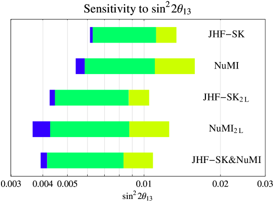
Figure 1: The $\sin^{2}2\theta_{13}$ sensitivity limits for the JHF-SK and NuMI experiments at normal and double luminosity (2L), as well as their combination ($90\%$ confidence level, LMA values). The left edges of the bars correspond to the sensitivity limits from statistics only. The right edges of the bars correspond to the real sensitivity limits after switching on systematics (blue), correlations (green), and degeneracies (yellow) successively from the left to the right.

Figure 1 shows the $\sin^{2}2\theta_{13}$ sensitivity limits for the JHF-SK and NuMI experiments at single and double luminosities and for their combination (with the individual experiments at single luminosity). The left edges of the bars correspond to the sensitivity limits from statistics, while the right edges correspond to the sensitivity limits after successively switching on systematics, correlations, and degeneracies (from left to right). We obtain these plots by finding the largest value of $\sin^{2}2\theta_{13}$ which fits the true $\sin^{2}2\theta_{13}=0$ at the selected confidence level. For the cases of correlations and degeneracies, any solution fitting $\sin^{2}2\theta_{13}=0$ has to be taken into account, since it cannot be distinguished from the best-fit solution. It is important to understand that, without better external information at this time, there is no argument to circumvent this definition and thus no pessimistic choice in that, since a limit is by definition a one-sided interval of all values compatible with a null result. The actual sensitivity limits are therefore the rightmost edges of the bars. Nevertheless, we still find it useful to plot the influence of systematics, correlations, and degeneracies, because these plots demonstrate where the biggest room for optimization is.

For the separate JHF-SK and NuMI experiments at normal luminosity, Figure 1 demonstrates that both experiments are approximately equal before the inclusion of systematics, correlations, and degeneracies (left edges of bars). In fact, the NuMI experiment performs somewhat better. However, the real sensitivity limits at the right edges of the bars are slightly different, i.e., the NuMI experiment is somewhat worse, especially because of the $\mathrm{sgn}(\Delta m_{31}^{2})$ degeneracy. In order to discuss the synergy effects of their combination, we argued in Section 2 that comparing the experiments at the normal (single) luminosity with their combination does mainly take into account the luminosity increase, i.e., the better statistics. Thus, we show in Figure 1 the experiments at double luminosity and their combination. It turns out that their combination (at single luminosity) is approximately as good as the JHF-SK experiment at double luminosity, mainly due to the reduction of the degeneracy error in the NuMI experiment. Nevertheless, this sort of analysis demonstrates that there are no big surprises to expect in building experiments optimized for a similar $L/E$. Obviously, both experiments combined will do better than each of the individual experiments because of the better statistics, but we do not observe a synergy effect when comparing the combination to the individual double luminosity upgrades.

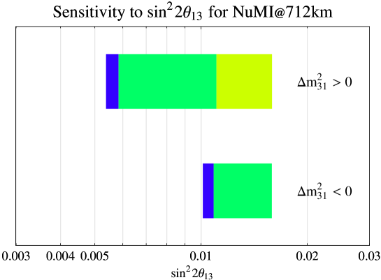
Figure 2: The $\sin^{2}2\theta_{13}$ sensitivity limits for the NuMI experiment for positive and negative signs of $\Delta m_{31}^{2}$ ($90\%$ confidence level, LMA values). The left edges of the bars correspond to the sensitivity limits from statistics only. The right edges of the bars correspond to the real sensitivity limits after switching on systematics (blue), correlations (green), and degeneracies (yellow) successively from the left to the right.

Another interesting issue is that, in this definition, the final sensitivity limits for positive and negative signs of $\Delta m_{31}^{2}$ are equal because the true rate vectors for $\sin^{2}2\theta_{13}=0$ are identical. This is demonstrated in Figure 2 for the example of the NuMI experiment and can be understood by looking at the sensitivity limits for the different signs: for the positive sign of $\Delta m_{31}^{2}$, the purely statistical sensitivity limit (left edge of bars) is somewhat better than the one for the negative sign of $\Delta m_{31}^{2}$. After the inclusion of correlations, there is still a degenerate solution with the negative sign of $\Delta m_{31}^{2}$ making the sensitivity limit worse, which appears as degeneracy part in the bars. From the point of view of a negative sign of $\Delta m_{31}^{2}$, however, the degenerate solution appears at $+|\Delta m_{31}^{2}|$ and is somewhat better than the sensitivity limit at the best-fit point at $-|\Delta m_{31}^{2}|$ . Thus, there is no degeneracy which makes the solution worse. Both the sensitivity limits for $\pm|\Delta m_{31}^{2}|$ are for our experiments therefore determined by the negative sign solution leading to an equal final sensitivity limit. We will therefore show later only the results for $+|\Delta m_{31}^{2}|$ and keep in mind that the final sensitivity limits for $\pm|\Delta m_{31}^{2}|$ are equal.

As already mentioned, the $\sin^{2}2\theta_{13}$ sensitivity strongly depends on the true value of $\Delta m_{31}^{2}$. One may ask, if both experiments combined could reduce the risk of not knowing $\Delta m_{31}^{2}$ precisely, i.e., flatten the curve describing the $\Delta m_{31}^{2}$ dependence of the $\sin^{2}2\theta_{13}$ sensitivity limit. This dependence is shown in Figure 3 for the experiments at double luminosity and their combination in order to be immediately able to compare the performance of the individual experiments to their combination. It includes systematics, correlations, and degeneracies.

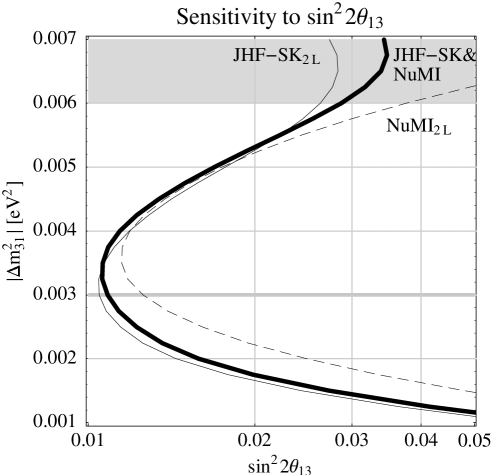
Figure 3: The $\sin^{2}2\theta_{13}$ excluded regions (on the right-hand sides of the contours) as function of $\Delta m_{31}^{2}$ (90% confidence level, LMA values). The curves show JHF-SK_2L (thin solid curve), NuMI_2L (thin dashed curve), and JHF-SK and NuMI combined (thick curve), where JHF-SK_2L and NuMI_2L refer to JHF-SK and NuMI, respectively, at double luminosity. The atmospheric excluded region is shaded in gray as well as the best-fit value is shown as the gray line. The shown sensitivity limits include systematics, correlations, and degeneracies.

First of all, it demonstrates that both experiments are optimized for the current best-fit value $\Delta m_{31}^{2}\simeq 3.0\cdot 10^{-3}\,\mathrm{eV}^{2}$, since in this region both experiments perform best. At somewhat larger values of $\Delta m_{31}^{2}$, NuMI is slightly better, and at the best-fit value and somewhat smaller values of $\Delta m_{31}^{2}$, JHF-SK is somewhat better, essentially because of the $\mathrm{sgn}(\Delta m_{31}^{2})$ degeneracy affecting the NuMI results. In addition, it shows that the combination of the two experiments would be almost as good as the best of the two. There is thus no real synergy, i.e., one could (theoretically) run JHF-SK ten years instead of five or use twice the detector mass in order to obtain similar results to the combination of both experiments.

Two other parameters could be of interest to superbeam experiments: the sign of $\Delta m_{31}^{2}$ and (maximal) CP violation, as a representative of the $\delta_{\mathrm{CP}}$ measurements. However, for the setups discussed in this section, we find only marginal sensitivities. The sign of $\Delta m_{31}^{2}$ can not be measured at all with the setups in this section, neither with the individual initial stage JHF-SK or NuMI experiments, nor with their double luminosity upgrades, nor with their combination. In addition, the CP violation sensitivity is, in the individual experiments, essentially not present in the LMA allowed region. For the combination of the experiments, we only obtain a marginal sensitivity at very high values of $\Delta m_{21}^{2}$. For a comparison of the JHF-SK to other long baseline experiments, such as the JHF to Hyper-Kamiokande upgrade and neutrino factories, see also Ref. [47].

In summary, we have seen that the JHF-SK and NuMI experiments, as they are planned right now, both have a quite similar $\sin^{2}2\theta_{13}$ sensitivity much below the CHOOZ bound, bot no sensitivity to the sign of $\Delta m_{31}^{2}$ and only a marginal sensitivity to CP violation. Thus, both experiments are essentially doing the same sort of physics. In the next section, we will thus raise the question if a combination of both experiments under doable modifications can do a much richer physics, i.e., measure the sign of $\Delta m_{31}^{2}$ or CP violation.

6 Alternative options for the combination of the experiments

It is interesting to study if it is possible to do more ambitious physics with the initial stage NuMI and JHF-SK experiments together than we found in the last section, i.e., if it is possible to measure the sign of $\Delta m_{31}^{2}$ or CP violation. The price to pay for that could be that (at least) one of the experiments performs worse with respect to the main parameters $\Delta m_{31}^{2}$, $\theta_{23}$, and $\sin^{2}2\theta_{13}$. Thus, we will first discuss alternative options for both experiments in order to measure the sign of $\Delta m_{31}^{2}$ or CP violation. Then, we will investigate what modifications of the experiments mean for the sensitivity limit of $\sin^{2}2\theta_{13}$ as one of the most important goals of these experiments.

Before we come to the individual parameter measurements, we need to clarify what we understand under alternative options for the initial stage experiments. Since the Super-Kamiokande detector exists already and the NuMI decay pipe is already built, the most reasonable options for modifications are the NuMI baseline (with a certain off-axis angle) and the possibility of antineutrino running for both experiments, where the NuMI baseline length and off-axis angle cannot be optimized independently because of the already installed decay pipe. For a fixed off-axis angle, the possible detector sites lie on an ellipse on the Earth’s surface. Since, besides other constraints, a possible detector site requires infrastructure and it turns out that the physics potential of both experiments is essentially in favor of a longer NuMI baseline, we choose two additional candidates with a baseline much longer than $712\,\mathrm{km}$. One is at a baseline length of $L=890\,\mathrm{km}$ at an off-axis angle of $0.72^{\circ}$, which is the longest possible choice for this off-axis angle.

	JHF-SK		NuMI				Combined
No.	$\nu$	$\bar{\nu}$	$\nu$	$\bar{\nu}$	L [km]	OA angle	Label
1	1	0	1	0	712	0.72∘	712$\nu\nu$
2	1	0	1	0	890	0.72∘	890$\nu\nu$
3	1	0	1	0	950	0.97∘	950$\nu\nu$
4	2/8	6/8	2/7	5/7	712	0.72∘	712cc
5	2/8	6/8	2/7	5/7	890	0.72∘	890cc
6	2/8	6/8	2/7	5/7	950	0.97∘	950cc
7	1	0	0	1	712	0.72∘	712$\nu\bar{\nu}$
8	1	0	0	1	890	0.72∘	890$\nu\bar{\nu}$
9	1	0	0	1	950	0.97∘	950$\nu\bar{\nu}$
10	0	1	1	0	712	0.72∘	712$\bar{\nu}\nu$
11	0	1	1	0	890	0.72∘	890$\bar{\nu}\nu$
12	0	1	1	0	950	0.97∘	950$\bar{\nu}\nu$

Table 3: The tested alternative scenarios for the combination of the JHF-SK and NuMI experiments. The columns refer to: the scenario number, the neutrino and antineutrino running fractions $\nu$ and $\bar{\nu}$ for the individual experiments, the NuMI baseline length $L$, the NuMI off-axis angle, and the labels used in the following plots.

A possible detector site is Fort Frances, Ontario, with a baseline $L=875\,\mathrm{km}$ [64]. The other candidate is at a baseline length of $L=950\,\mathrm{km}$ at an off-axis angle of $0.97^{\circ}$. It has a longer baseline with a larger off-axis angle, i.e., with larger matter effects and the spectrum is sharper peaked but the statistics is worse. A possible site at exactly this baseline is Vermilion Bay, Ontario. For the running with inverted polarities, we investigate options with neutrino running in both JHF-SK and NuMI, neutrino running in JHF-SK and antineutrino running in NuMI or vice versa, and combinations of neutrino and antineutrino running in both JHF-SK and NuMI with a splitting of the running time such that we approximately have the same numbers of neutrino and antineutrino events, i.e., 2/8 of neutrino running and 6/8 of antineutrino running at JHF-SK and 2/7 of neutrino running and 5/7 of antineutrino running at NuMI. The tested scenarios are listed in Table 3 and we will further on use the labels shown in the column “Label” to identify the different scenarios. The labels refer to the NuMI baseline length, the JHF-SK polarity (first letter) and the NuMI polarity (second letter), where the abbreviation “$\nu$” stands for neutrino running only, “$\bar{\nu}$” for antineutrino running only, and “c” for the combined option.

6.1 The measurement of the sign of $\Delta m_{31}^{2}$

One possibility to broaden the physics potential is to measure the sign of $\Delta m_{31}^{2}$. Recent studies, such as Ref. [47], demonstrate that it is very hard to access this parameter even at high-luminosity superbeam upgrades (such as JHF to Hyper-Kamiokande) or neutrino factories essentially due to the $\mathrm{sgn}(\Delta m_{31}^{2})$ degeneracy. However, the combination of two complementary baselines can help to resolve this degeneracy. Especially, a very long baseline with large matter effects adds a lot to the sensitivity, though it is not optimal as a standalone setup because of the lower statistics.

Before we present our analysis, we define the sensitivity to the sign of $\Delta m_{31}^{2}$ and describe how we evaluate it. Sensitivity to a certain sign of $\Delta m_{31}^{2}$ exists if there is no solution with the opposite sign which fits the true values at the chosen confidence level. It is essential to understand that if we find such a solution, we will not be able to measure the sign of $\Delta m_{31}^{2}$, because the new solution opens the possibility of a completely new parameter set at $\simeq\,-\Delta m_{31}^{2}$ which cannot be distinguished from the best-fit one. Thus, finding such a degenerate solution proofs that there is no sensitivity to the sign of $\Delta m_{31}$ at the chosen best-fit parameter values. Practically, we are scanning the half of the parameter space with the inverted $\Delta m_{31}^{2}$ for the $\mathrm{sgn}(\Delta m_{31}^{2})$ degeneracy. We do not find the degenerate solution exactly in the $(\delta_{\mathrm{CP}},\theta_{13})$-plane at $-\Delta m_{31}^{2}$, since it can lie slightly off this plane. This makes it necessary to use a local minimum finder in the high dimensional parameter space, which, for example, can be started in the $(\delta_{\mathrm{CP}},\theta_{13})$-plane at $-\Delta m_{31}^{2}$ and then runs down into the local minimum off the plane. In other words, the sign of $\Delta m_{31}^{2}$ measurement is also correlated with the other parameter measurements. Moreover, it turns out that the actual value of $\delta_{\mathrm{CP}}$ strongly determines the sign of $\Delta m_{31}^{2}$ sensitivity. Since $\delta_{\mathrm{CP}}$ will not be measured before the considered experiments, the only information on $\delta_{\mathrm{CP}}$ can come from the experiments themselves, i.e., we assume that we do not know $\delta_{\mathrm{CP}}$ a priori. For a certain parameter set, the actual value of $\delta_{\mathrm{CP}}$ will determine the confidence level at which the degenerate solution appears. Since, in some sense, without a priori measurement all values of $\delta_{\mathrm{CP}}$ are equally favored, we compute the sign of $\Delta m_{31}^{2}$ sensitivity for all possible value of $\delta_{\mathrm{CP}}$ and take the worst case. Thus, our regions show where we are sensitive to the sign of $\Delta m_{31}^{2}$ in either case of $\delta_{\mathrm{CP}}$. Another issue is that there is a slight difference in the measurement of the sign of $\Delta m_{31}^{2}$ and the sensitivity to a positive or negative sign of $\Delta m_{31}^{2}$. We ask for the sensitivity to a positive or negative sign of $\Delta m_{31}^{2}$ and show the regions were this sign could be verified. To measure the sign of $\Delta m_{31}^{2}$ would mean to proof its value in either case, i.e., one had to take the worst case of the sensitivity regions for positive and negative signs.

As a first result of this analysis, we find, as indicated in the last section, no sensitivity to the sign of $\Delta m_{31}^{2}$ neither for JHF-SK or NuMI (at $712\,\mathrm{km}$ with neutrino running only) at single or double luminosity, nor for their combination. However, we find that increasing the NuMI baseline leads to sensitivity at baselines of $L\gtrsim 800\,\mathrm{km}$. The optimum at approximately the second oscillation maximum at $L\sim 1400\,\mathrm{km}$, which can, however, not be reached by the fixed decay pipe and does not give a good sensitivity to $\sin^{2}2\theta_{13}$ anymore. Thus, we take the above introduced baseline-off-axis angle combinations at $890\,\mathrm{km}$ and $950\,\mathrm{km}$ with the neutrino-antineutrino running time combinations of JHF-SK and NuMI listed in Table 3.

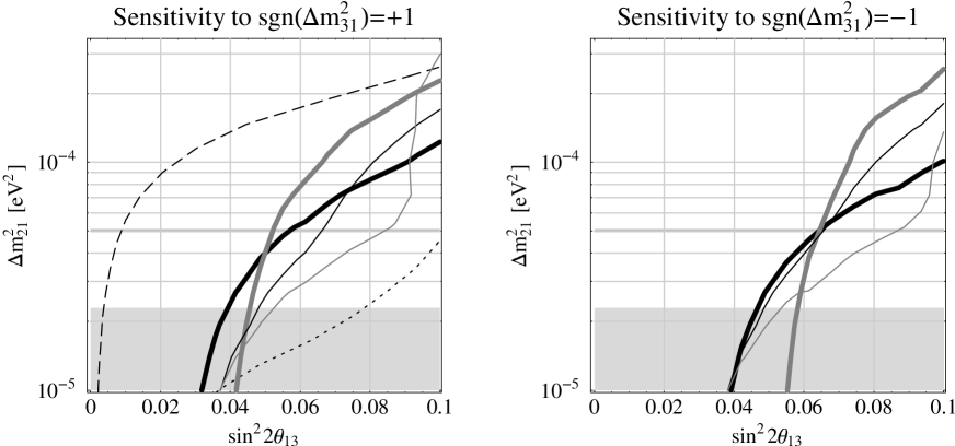
Figure 4: The sensitivity regions to a positive (left-hand plot) and negative (right-hand plot) sign of $\Delta m_{31}^{2}$ as functions of $\sin^{2}2\theta_{13}$ and $\Delta m_{21}^{2}$ ($90\%$ confidence level, LMA values), where sensitivity exists on the right-hand side of the curves. In the plots, the curves for JHF-SK and NuMI combined are shown for the following options, listed in Table 3: $890\nu\nu$ (thick gray curve), $950\nu\nu$ (thick black curve), $890cc$ (thin gray curve), and $950cc$ (thin black curve). In addition the NuFact-I (initial stage neutrino factory, dashed curve) and JHF-HK (JHF to Hyper-Kamiokande superbeam upgrade, dotted curve) setups from Ref. [47] are shown for comparison in the left-hand plot. The gray horizontal line marks the LMA best-fit value, whereas the gray-shaded region corresponds to the current LMA excluded region.

Figure 4 shows the sensitivity to a positive (left-hand plot) or negative (right-hand plot) sign of $\Delta m_{31}^{2}$ for the best of these options. We do not show the scenarios with running one of the experiments with antineutrinos only, because this reduces the reach in $\Delta m_{21}^{2}$ severely. The reduction of the sensitivity at larger values of $\Delta m_{21}^{2}$ comes, as described in Section 4, essentially from the larger CP-effects, above a certain threshold value in $\Delta m_{21}^{2}$ we are not sensitive to the sign of $\Delta m_{31}^{2}$ anymore. As the main result, we find that running both beams with neutrinos only at a NuMI baseline of $890\,\mathrm{km}$ or $950\,\mathrm{km}$ gives the best results, where the sensitivity for a negative sign of $\Delta m_{31}^{2}$ is slightly worse. Above $\Delta m_{21}^{2}\simeq 4.5\cdot 10^{-5}\,\mathrm{eV^{2}}$ the $890\,\mathrm{km}$ option with the smaller off-axis angle performs better, whereas below $\Delta m_{21}^{2}\simeq 4.5\cdot 10^{-5}\,\mathrm{eV^{2}}$ the $950\,\mathrm{km}$ option with the larger off-axis angle is better.

	JHF-SK			NuMI				Combined
No.	$\nu$	$\bar{\nu}$	Sensitivity	$\nu$	$\bar{\nu}$	L [km]	Sensitivity	Label	Sensitivity
1	1	0	None	1	0	712	None	712$\nu\nu$	None
2	1	0	None	1	0	890	None	890$\nu\nu$	Good
3	1	0	None	1	0	950	None	950$\nu\nu$	Good
4	2/8	6/8	None	2/7	5/7	712	Marginal	712cc	Marginal
5	2/8	6/8	None	2/7	5/7	890	Marginal	890cc	Poor
6	2/8	6/8	None	2/7	5/7	950	Marginal	950cc	Good
7	1	0	None	0	1	712	None	712$\nu\bar{\nu}$	Marginal
8	1	0	None	0	1	890	None	890$\nu\bar{\nu}$	Poor
9	1	0	None	0	1	950	None	950$\nu\bar{\nu}$	Poor
10	0	1	None	1	0	712	None	712$\bar{\nu}\nu$	Marginal
11	0	1	None	1	0	890	None	890$\bar{\nu}\nu$	Poor
12	0	1	None	1	0	950	None	950$\bar{\nu}\nu$	Poor

Table 4: The sign of $\Delta m_{31}^{2}$ sensitivity (qualitatively) for the tested alternative options for the individual JHF-SK and NuMI experiments (normal luminosity), as well as their combination. The columns refer to: the scenario number, the neutrino and antineutrino running fractions $\nu$ and $\bar{\nu}$ for the individual experiments, the NuMI baseline length $L$, and the label of the combined experiments. The sensitivity reaches are classified as “None” (no sensitivity), “Marginal” (sensitivity only in lower right corner in plots in Figure 4), “Poor” (good maximal reach in $\sin^{2}2\theta_{13}$ or $\Delta m_{21}^{2}$, but area covered in plots in Figure 4 relatively small), and “Good” (good coverage in $\sin^{2}2\theta_{13}$ and $\Delta m_{21}^{2}$ reach as well as area). The best options are also shown in Figure 4.

Table 4 summarizes our performance tests for the sign of $\Delta m_{31}$ qualitatively. Comparing the sensitivity regions to future high luminosity superbeam upgrades or initial stage neutrino factories (cf., left-hand plot), we could achieve relatively good sensitivities to the sign of $\Delta m_{31}^{2}$ even with the initial stage setups. As far as the dependence on the true value of $\Delta m_{31}^{2}$ is concerned, a larger value of ${\Delta m^{2}_{31}}$ increases the resonance energy and therefore reduces the matter effects. However, a larger value of ${\Delta m^{2}_{31}}$ allows a higher energy in order to overcompensate the smaller matter effects and to finally obtain somewhat better results. The same arguments also work for smaller values of ${\Delta m^{2}_{31}}$. In this case, however, an experiment, even if it is fully optimized for this lower value, strongly suffers from the loss in statistics since increasing the baseline or lowering the energy strongly reduces the number of events.

6.2 The sensitivity to CP violation

Another alternative for optimization with the combined JHF-SK and NuMI experiments under modified conditions is leptonic CP violation. We restrict the discussion to maximal CP violation, i.e., $\delta_{\mathrm{CP}}=\pm\pi/2$, but one could also discuss connected topics, such as the precision of the $\delta_{\mathrm{CP}}$ measurement or the establishment of CP violation for CP phases closer to CP conservation, i.e., $\delta_{\mathrm{CP}}=0$ or $\pi$. However, we expect the qualitative behavior for these problems to be similar and choose the sensitivity to maximal CP violation as representative.

For our analysis, we compute the degenerate solution in $\mathrm{sgn}(\Delta m_{31}^{2})$ as discussed in the last section, since it turns out that this degeneracy can have a CP phase very different from the original solution [47]. The question of the sensitivity to maximal CP violation can be answered by setting the CP phase to $\delta_{\mathrm{CP}}=+\pi/2$ or $\delta_{\mathrm{CP}}=-\pi/2$ and computing the four $\chi^{2}$-values at the best-fit and degenerate solution for $\delta_{\mathrm{CP}}=0$ and $\pi$, respectively. For the case of antineutrino running, the additional possible ambiguity in the $(\delta_{\mathrm{CP}},\theta_{13})$-plane is taken into account. If one of the computed $\chi^{2}$-values is under the threshold for the selected confidence level, maximal CP violation cannot be established for the evaluated parameter set.

Before we discuss the options introduced in Table 3, we want to compare the performance of the individual JHF-SK and NuMI experiments at double luminosity to their combination. Figure 5 shows the sensitivity to maximal CP violation $\delta_{\mathrm{CP}}=+\pi/2$ for $\Delta m_{31}^{2}>0$ as function of $\sin^{2}2\theta_{13}$ and $\Delta m_{21}^{2}$, since we find that there are no interesting qualitative differences for $\delta_{\mathrm{CP}}=-\pi/2$ or $\Delta m_{31}^{2}<0$. In this figure, the curves for JHF-SK_2L and NuMI_2L (at double luminosity) for neutrino running only, as well as their combination with NuMI at $L=712\,\mathrm{km}$ with combined neutrino-antineutrino running (Scenario “712cc” in Table 3) are shown.

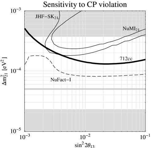
Figure 5: The sensitivity to maximal CP violation $\delta_{\mathrm{CP}}=+\pi/2$ for $\Delta m_{31}^{2}>0$ as function of $\sin^{2}2\theta_{13}$ and $\Delta m_{21}^{2}$ (90% confidence level, LMA values). The curves for JHF-SK_2L and NuMI_2L at double luminosity with neutrino running only, as well as the curve for both combined ($712cc$) are shown. All curves are plotted for the NuMI baseline of $712\,\mathrm{km}$. In addition, we show the result for the NuFact-I scenario (initial stage neutrino factory) from Ref. [47] for comparison as dashed curve. The LMA excluded region is shaded in gray and its best-fit value is marked by the gray horizontal line.

One can easily see that the combination of the two experiments under somewhat modified conditions (antineutrino running included) leads to a much better coverage of the $\sin^{2}2\theta_{13}$-$\Delta m_{21}^{2}$-plane, which cannot be explained by the statistics increase only. In this case, one could talk about a synergy between the two experiments. It turns out that most of the alternative options including antineutrino running, if not put exclusively to JHF-SK, are performing similarly well. Thus, we show in Figure 6 the sensitivity to maximal CP violation for the two options of combined neutrino and antineutrino running with a NuMI baseline of $712\,\mathrm{km}$ and $890\,\mathrm{km}$.

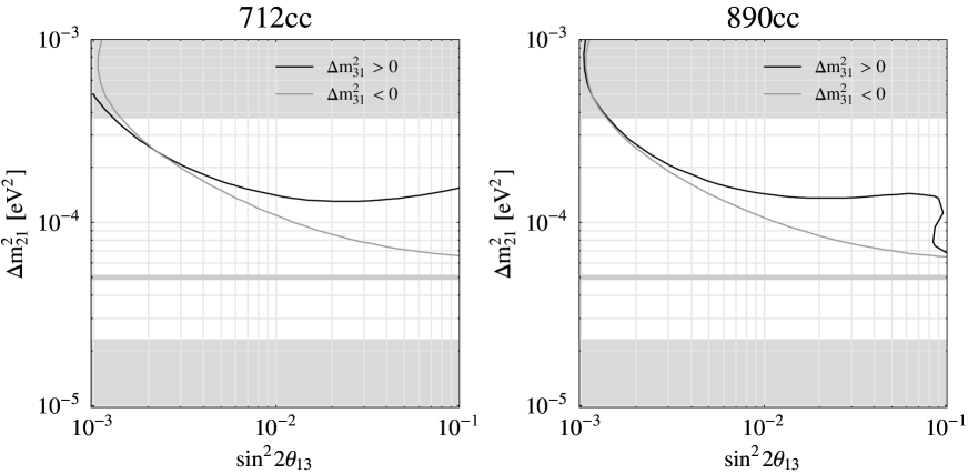
Figure 6: The sensitivity to maximal CP violation $\delta_{\mathrm{CP}}=+\pi/2$ for $\Delta m_{31}^{2}>0$ (black curves) and $\Delta m_{31}^{2}<0$ (gray curves) as functions of $\sin^{2}2\theta_{13}$ and $\Delta m_{21}^{2}$ (90% confidence level, LMA values). The left-hand plot shows the sensitivity for the combined experiments and NuMI at $712\,\mathrm{km}$ ($712cc$) and the right-hand plot for NuMI at $890\,\mathrm{km}$ ($890cc$), both with combined neutrino and antineutrino running. The LMA excluded region is shaded in gray and its best-fit value is marked by the gray horizontal line.

In this figure, essentially all curves for the scenarios classified as “Good” in Table 5 summarizing the results of this analysis qualitatively, are very close to the ones plotted for $\Delta m_{31}^{2}>0$ and $\Delta m_{31}^{2}<0$, respectively. In addition, there is no big difference between choosing $\delta_{\mathrm{CP}}=+\pi/2$ and $\delta_{\mathrm{CP}}=-\pi/2$. However, the results for the $950\,\mathrm{km}$ NuMI baseline are slightly worse. In summary, we find that for the detection of maximal CP violation all combinations which include a substantial fraction of antineutrino running perform very well – except from the option of running NuMI with neutrinos only and JHF-SK with antineutrinos only.

	JHF-SK			NuMI				Combined
No.	$\nu$	$\bar{\nu}$	Sensitivity	$\nu$	$\bar{\nu}$	L [km]	Sensitivity	Label	Sensitivity
1	1	0	None	1	0	712	None	712$\nu\nu$	Poor
2	1	0	None	1	0	890	None	890$\nu\nu$	Poor
3	1	0	None	1	0	950	None	950$\nu\nu$	Poor
4	2/8	6/8	None	2/7	5/7	712	None	712cc	Good
5	2/8	6/8	None	2/7	5/7	890	None	890cc	Good
6	2/8	6/8	None	2/7	5/7	950	None	950cc	Suboptimal
7	1	0	None	0	1	712	None	712$\nu\bar{\nu}$	Good
8	1	0	None	0	1	890	None	890$\nu\bar{\nu}$	Good
9	1	0	None	0	1	950	None	950$\nu\bar{\nu}$	Suboptimal
10	0	1	None	1	0	712	None	712$\bar{\nu}\nu$	Poor
11	0	1	None	1	0	890	None	890$\bar{\nu}\nu$	Poor
12	0	1	None	1	0	950	None	950$\bar{\nu}\nu$	Poor

Table 5: The CP violation sensitivity (qualitatively) for the tested alternative options for the individual JHF-SK and NuMI experiments (normal luminosity), as well as their combination. The columns refer to: the scenario number, the neutrino and antineutrino running fractions $\nu$ and $\bar{\nu}$ for the individual experiments, the NuMI baseline length $L$, and the label of the combined experiments. The sensitivity reaches are classified in “None” (no or only marginal sensitivity in the LMA range), “Poor” (good reach in $\sin^{2}2\theta_{13}$ or $\Delta m_{21}^{2}$, but area covered in plots in Figure 6 relatively small), “Suboptimal” (fairly good, but not optimal coverage in area), and “Good” (good coverage in area). The options classified with “Good” correspond to the curves shown in Figure 6.

The qualitative behavior can be understood from Equation (1), where the second and third terms contribute most to the CP violation sensitivity. They are both getting the largest relative weight if both $\sin^{2}2\theta_{13}$ and $\Delta m_{21}^{2}$ are rather large, whereas they are suffering from the large absolute background from the first term if $\Delta m_{21}^{2}$ is too small. Thus, we could only measure CP violation in the so-called HLMA-region, i.e., at the upper end of the LMA range. As far as the dependence on the value of ${\Delta m^{2}_{31}}$ is concerned, a larger value of ${\Delta m^{2}_{31}}$ would imply a lower value of $\alpha$ in Equation (1) and thus decrease the relative strength of CP effects. However, it would allow to choose a shorter baseline or higher energy, which both increase the total event rates. This improvement in statistics has more relative weight than the reduction of the CP effects. For lower values of ${\Delta m^{2}_{31}}$, it is very hard to improve the results by optimizing the energy or baseline, since, such as for the sign of $\Delta m_{31}^{2}$ measurement, the statistics always decreases and thus makes the measurement difficult.

6.3 The sensitivity to $\sin^{2}2\theta_{13}$

We have seen that there are several alternative options for the combination of the JHF-SK and NuMI experiments. We have also indicated that a different setup could make the measurement of $\sin^{2}2\theta_{13}$ worse. Thus, we show in Figure 7 how much the sensitivity is changed for a selected set of the alternative options as well as the original combination at $712\,\mathrm{km}$ (first bar).

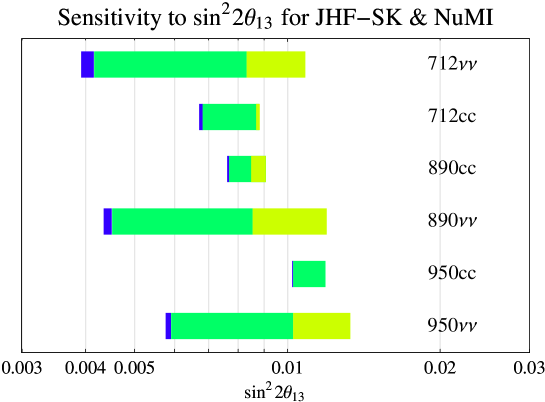
Figure 7: The $\sin^{2}2\theta_{13}$ sensitivity limits ($90\%$ confidence level, LMA values) for the combined JHF-SK and NuMI experiments for a selected set of the alternative options and the original combination (first bar). The labels are defined in Table 3. The left edges of the bars correspond to the sensitivity limits from statistics only. The right edges of the bars correspond to the real sensitivity limits after switching on systematics (blue), correlations (green), and degeneracies (yellow) successively from the left to the right.

The sensitivity limit is, in all cases, reduced due to statistics only (left edges of the bars). However, due to the reduction of correlations and degeneracies, i.e., partial complementarity of the different baselines and polarities, many of the setups perform even better after the inclusion of all error sources. In the end, any of the shown setups has a very good performance in the $\sin^{2}2\theta_{13}$ sensitivity. In addition, one has to keep in mind that the dependency on the atmospheric and solar mass squared differences can affect this result much stronger than choosing the suboptimal solution. For example, for larger values of $\Delta m_{21}^{2}$ these limits are shifted to higher values and for smaller values of $\Delta m_{21}^{2}$ the limits are shifted to smaller values. At about $\Delta m_{21}^{2}\simeq 3\cdot 10^{-4}\,\mathrm{eV}^{2}$ we would finally reach the CHOOZ bound. Since this value is still within the LMA allowed region, there is in the worst case no guarantee that a limit better than the CHOOZ could be obtained.

For the alternative options of the combined two experiments, one can again raise the question if it is possible to reduce the risk of having optimized for the wrong value of $|{\Delta m^{2}_{31}}|$. We find that spreading the $L/E$ values of the two experiments, i.e., having one experiment somewhat below the first maximum at $|{\Delta m^{2}_{31}}|=3.0\cdot 10^{-3}\,\mathrm{eV}^{2}$ and the other above, would only improve the $\sin^{2}2\theta_{13}$ sensitivity limit for $|{\Delta m^{2}_{31}}|>3.0\cdot 10^{-3}\,\mathrm{eV}^{2}$. This can, in general, be understood in terms of the scaling of the statistics. Increasing the value of $|{\Delta m^{2}_{31}}|$ would mean shifting the first maximum to higher energies or shorter baselines. For the case of higher energies, the event rates, scaling $\propto E^{3+x}$, would be increased. For the case of shorter baselines, the rates simply scale $\propto 1/L^{2}$. Thus, any of the two options would lead to higher event rates for an experiment optimized for a larger value of $|{\Delta m^{2}_{31}}|$. The same reasoning for lower values of $|{\Delta m^{2}_{31}}|$ always results in much lower event rates. Thus, even an experiment optimized for this lower value of $|{\Delta m^{2}_{31}}|$ tends to perform much worse in absolute numbers. From calculations, we find that for $|{\Delta m^{2}_{31}}|=5.0\cdot 10^{-3}\,\mathrm{eV}^{2}$ the sensitivity limit could be relatively improved by $\simeq 50\%$ (linear scale) compared to the standard setup 712$\nu\nu$ without loosing much at lower values of $|{\Delta m^{2}_{31}}|$. This result is, however, obtained for unrealistic values of the baselines, which means that for a realistic setup the improvement will be smaller. For $|{\Delta m^{2}_{31}}|=1.0\cdot 10^{-3}\,\mathrm{eV}^{2}$, the best result would also be approximately $50\%$ better. However, his effect almost vanishes already at $|{\Delta m^{2}_{31}}|\sim 1.5\cdot 10^{-3}\,\mathrm{eV}^{2}$. Thus, we conclude that there does not seem to be much improvement by fine tuning the combination of experiments for the reduction of the risk – given all constraints on baselines and off-axis angles.

7 Summary and conclusions

In this paper, we have first presented an analysis of the JHF-SK and NuMI superbeam experiments as they are proposed in their letters of intent. We demonstrated that both are optimized under similar conditions, i.e., for a similar value of $L/E$, in order to measure the leading atmospheric parameters and $\sin^{2}2\theta_{13}$ at the current atmospheric best-fit values. However, we have also shown that there are no real synergy effects in these two experiments, i.e., effects which go beyond the simple addition of statistics. A combined fit of their data shows only the improvement of the results coming from the better statistics, which is not surprising since two similar experiments combined simply perform better than one. To demonstrate this, we have plotted their individual results at double luminosities and we have compared them to their combined fit. Their combined results for $\sin^{2}2\theta_{13}$ are approximately as good as the best of the individual ones at double luminosity, even as a function of $\Delta m_{31}^{2}$. In addition, we have not found any sensitivity to the sign of $\Delta m_{31}^{2}$, neither in the individual experiments, nor in their combination. Moreover, there is hardly any sensitivity to CP violation in the LMA allowed region. Thus, we conclude that for the current design as specified in the LOIs one could run one experiment equally well twice as long as planned (or with a twice as big detector) instead of building a second experiment.

As alternatives to the originally considered setups, we have proposed to run either one or both of the two experiments partly or entirely with antineutrinos, or to build the NuMI detector at a different baseline. We especially considered two alternative baselines of $890\,\mathrm{km}$ at an off-axis angle of 0.72^∘ and $950\,\mathrm{km}$ at an off-axis angle of 0.97^∘, which both would be still possible under the constraint of the fixed NuMI decay pipe. Possible detector sites for these baselines are Fort Frances, Ontario ($L=875\,\mathrm{km}$) and Vermilion Bay, Ontario ($L=950\,\mathrm{km}$). We have found that, under such modified conditions, one could then either measure the sign of $\Delta m_{31}^{2}$ or (maximal) CP violation, depending on the actual value of $\Delta m_{21}^{2}$, by combining the initial stage JHF-SK and NuMI experiments, i.e., with running times of five years each and detector masses as proposed in the letters of intent.

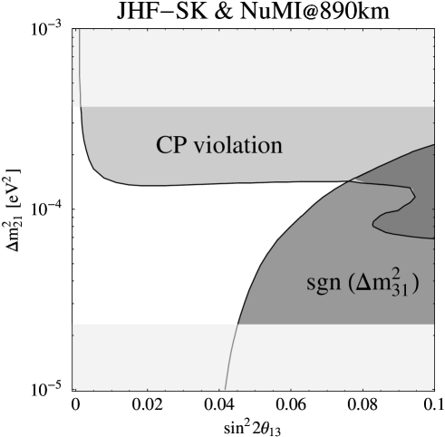
Figure 8: The regions of sign of $\Delta m_{31}^{2}$ and CP violation sensitivity (JHF-SK and NuMI combined) in the $\sin^{2}2\theta_{13}$-$\Delta m_{21}^{2}$-plane (90% confidence level, LMA values) for the $890\nu\nu$ (for the sign of $\Delta m_{31}^{2}$, neutrino running only) and $890cc$ (for CP violation, combined neutrino-antineutrino running) setups, where the LMA excluded region is shaded in gray.

Figure 8 shows the regions of sign of $\Delta m_{31}^{2}$ and CP violation sensitivity in the $\sin^{2}2\theta_{13}$-$\Delta m_{21}^{2}$-plane at the 90% confidence level for the $890\nu\nu$ (sign of $\Delta m_{31}^{2}$) and $890cc$ (CP violation) setups as defined in Table 3. One can easily see that, with these initial stage experiments, a simultaneous measurement of both quantities is hard to achieve. Thus, the strategy on what one wants to measure will strongly depend on the KamLAND result.

For the sign of $\Delta m_{31}^{2}$ sensitivity, the $890\,\mathrm{km}$ and $950\,\mathrm{km}$ options for the NuMI baseline with neutrino running only at both JHF-SK and NuMI turn out to perform very well. Above $\Delta m_{21}^{2}\sim 4.5\cdot 10^{-5}\,\mathrm{eV}^{2}$ the $890\,\mathrm{km}$ option does better (higher $\Delta m_{21}^{2}$ reach), below $\Delta m_{21}^{2}\sim 4.5\cdot 10^{-5}\,\mathrm{eV}^{2}$ the $950\,\mathrm{km}$ does better (better $\sin^{2}2\theta_{13}$ reach).

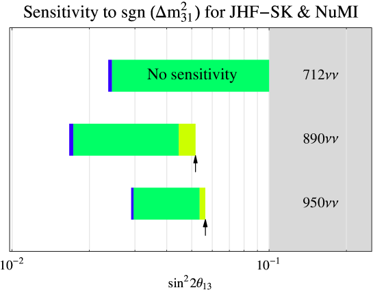
Figure 9: The sensitivity limits to the sign of $\Delta m_{31}^{2}$ in the direction of $\sin^{2}2\theta_{13}$ ($90\%$ confidence level, LMA values). The bars are shown for the combined JHF-SK and NuMI experiments for a selected set of the alternative options and the original combination (first bar), where the labels are explained in Table 3. The left edges of the bars correspond to the sensitivity limits from statistics only. The right edges of the bars correspond to the real sensitivity limits after switching on systematics (blue), correlations (green), and degeneracies (yellow) successively from the left to the right.

Figure 9 shows the sign of $\Delta m_{31}^{2}$ sensitivity limits at the LMA best-fit point for the original setup and the best of the alternative setups, including the influence of systematics, correlations, and degeneracies. In this figure, the left edges of the bars correspond to the sensitivity limits without taking into account the mentioned error sources, while successively switching on systematics, correlations, and degeneracies shifts the sensitivity limit to the right. Since it is very difficult to define the difference between correlations and degeneracies in this case, we fix $\delta_{\mathrm{CP}}=0$ at the border of the second and third bars. In either case, the right edges correspond to the real sensitivity limits. Thus, we do not have sensitivity to the sign of $\Delta m_{31}^{2}$ with the original setup, but we do have sensitivity at longer baselines. Which of the two proposed alternative baselines performs better depends on the exact value of $\Delta m_{21}^{2}$. However, from statistics only, the $890\,\mathrm{km}$ option is much better.

For the sensitivity to CP violation, the $712\,\mathrm{km}$ and $890\,\mathrm{km}$ baseline options for NuMI are performing very well – provided that $\Delta m_{21}^{2}$ is large enough and there is a substantial fraction of antineutrino running at NuMI (for a fixed total running time). Especially, running JHF-SK with neutrinos and NuMI with antineutrinos or running both experiments with neutrinos and antineutrinos with almost equal total numbers of neutrino and antineutrino events in each experiment provides very good results.

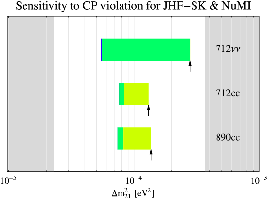
Figure 10: The sensitivity limits to (maximal) CP violation plotted in the direction of $\Delta m_{21}^{2}$ at the fixed value of $\sin^{2}2\theta_{13}=0.03$ ($90\%$ confidence level, LMA values). The bars are shown for the combined JHF-SK and NuMI experiments for a selected set of the alternative options and the original combination (first bar), where the labels are explained in Table 3. The left edges of the bars correspond to the sensitivity limits from statistics only. The right edges of the bars correspond to the real sensitivity limits after switching on systematics (blue), correlations (green), and degeneracies (yellow) successively from the left to the right. The gray-shaded are marks the region of the LMA excluded values.

Figure 10 shows the sensitivity limits to maximal CP violation for a fixed value of $\sin^{2}2\theta_{13}=0.03$ for the therein specified combinations and experiments, where again the systematics, correlations, an degeneracies are switched on from the left to the right. The right edges of the bars correspond thus to the final sensitivity limits. Especially the correlation of $\delta_{\mathrm{CP}}$ with $\theta_{13}$ can be resolved very well in this case with the alternative options. The remaining dominant error source comes then from the $\mathrm{sgn}(\Delta m_{31}^{2})$ degeneracy.

Summarizing these result, we find for the combination of the modified initial stage JHF-SK and NuMI experiments synergy effects, which means that they have the potential to do new physics for any value of $\Delta m_{21}^{2}$ in the LMA regime:

For $\Delta m_{21}^{2}\gtrsim 1.0\cdot 10^{-4}\,\mathrm{eV}^{2}$

one could be sensitive to (maximal) CP violation with a substantial fraction of antineutrino running at least in the NuMI experiment, or in both.

For $\Delta m_{21}^{2}\sim 4.5\cdot 10^{-5}\,\mathrm{eV}^{2}-\,1.0\cdot 10^{-4}\,\mathrm{eV}^{2}$

one would be optimally sensitive towards the sign of $\Delta m_{31}^{2}$ with a NuMI baseline of $\sim 890\,\mathrm{km}$ and running both JHF-SK and NuMI with neutrinos only.

For $\Delta m_{21}^{2}\lesssim 4.5\cdot 10^{-5}\,\mathrm{eV}^{2}$

one would be optimally sensitive towards the sign of $\Delta m_{31}^{2}$ with a NuMI baseline of $\sim 950\,\mathrm{km}$ and running both JHF-SK and NuMI with neutrinos only.

Especially, the options with a NuMI baseline of $L=890\,\mathrm{km}$ seems to be a good compromise independent of the forthcoming exact KamLAND results.

The proposed modifications for one or both of the experiments mean that the individual experiments are no longer optimized for the best-fit point by themselves anymore. They could therefore in many cases, as standalone experiments, not compete anymore with respect to the leading oscillation parameters. However, we have seen that the combined $\sin^{2}2\theta_{13}$ sensitivity limits, which in our definition do not depend on the sign of $\Delta m_{31}^{2}$, could even be better by up to $20\%$ and in the worst case the reduction would only be $10\%$. For the atmospheric parameters those modifications should not affect the result since any of the individual setups is systematics limited for this measurement. Thus, we conclude that it is possible to obtain exciting synergies for the combined JHF-SK and NuMI experiments if they are optimized together. Depending on $\Delta m_{21}^{2}$, the combination could then measure either the sign of $\Delta m_{31}^{2}$ or leptonic CP violation already within this decade.

Acknowledgments

We wish to thank Deborah A. Harris for valuable information on the NuMI experiment.

Appendix: Experiment Description

For the simulation of the experiments, we use the same techniques and notation as in Ref. [47]. Here we therefore only give a short description of each of the experiments and the numbers used in our calculation.

JHF-SK

The Super-Kamiokande detector has an excellent capability to separate muons and electrons. Furthermore, it provides a very accurate measurement of the charged lepton momentum [14]. However it is completely lacking the measurement of the hadronic fraction of a neutrino event. Therefore, the energy can only be reconstructed for the QE (quasi-elastic scattering) events. For this sort of events, the energy resolution is dominated by the Fermi motion of the nucleons, which induces a constant width of $80-100\,\mathrm{MeV}$ [14, 65]. In order to incorporate spectral information in our analysis, we use the spectrum of the QE events with a free normalization and the total rate of all CC (charged current) events. The free normalization of the spectrum is necessary to avoid double counting the QE events. For the energy resolution, we use a constant width of $\sigma_{E}=85\,\mathrm{MeV}$. The energy window for the analysis is $0.4-1.2\,\mathrm{GeV}$. The efficiencies and background fractions are given in Table 6 and taken from Ref. [14].

Disappearance
Signal	$0.9\otimes({\nu_{\mu}\rightarrow\nu_{\mu}})_{\mathrm{QE}}$
Background	$0.0056\otimes({\nu_{\mu}\rightarrow\nu_{x}})_{\mathrm{NC}}$
Appearance
Signal	$0.505\otimes({\nu_{\mu}\rightarrow\nu_{e}})_{\mathrm{CC}}$
Background	$0.0056\otimes({\nu_{\mu}\rightarrow\nu_{x}})_{\mathrm{NC}}$	$3.3\cdot 10^{-4}\otimes({\nu_{\mu}\rightarrow\nu_{\mu}})_{\mathrm{CC}}$
Beam background	$0.505\otimes({\nu_{e}\rightarrow\nu_{e}})_{\mathrm{CC}}$	$0.505\otimes({\bar{\nu}_{e}\rightarrow\bar{\nu}_{e}})_{\mathrm{CC}}$

Table 6: The efficiencies for the signals and backgrounds of the JHF-SK experiment.

We furthermore include a normalization uncertainty of $5\%$, as well as a background uncertainty of $5\%$. The results are however not sensitive to reasonable variations of those uncertainties, since the statistical error is much larger. The fluxes of $\nu_{\mu}$, $\nu_{e}$, and $\bar{\nu}_{e}$ are the ones corresponding to $2^{\circ}$ OA beam in [14] and have been provided as data file by Ref. [65].

NuMI

The NuMI detector used in our calculations is a low-Z calorimeter as described in Ref. [22]. It can measure both the lepton momentum and the hadronic energy deposition, albeit with different accuracies. The resolution is expected to be very similar to the MINOS detector [66]. Therefore we use a $\sigma_{E}=0.15\cdot E$, which has been shown in Ref. [47] to be a very good approximation to the MINOS resolution. The energy window for the analysis is $1.6-2.8\,\mathrm{GeV}$ for the $0.72^{\circ}$ off-axis beam and $1.2-2.5\,\mathrm{GeV}$ for the $0.97^{\circ}$ off-axis beam. The efficiencies and background fractions are given in Table 7 and are taken from Ref. [22] as far as they are given in there. The missing information was provided by Ref. [64].

Disappearance
Signal	$0.9\otimes({\nu_{\mu}\rightarrow\nu_{\mu}})_{\mathrm{CC}}$
Background	$0.005\otimes({\nu_{\mu}\rightarrow\nu_{x}})_{\mathrm{NC}}$
Appearance
Signal	$0.4\otimes({\nu_{\mu}\rightarrow\nu_{e}})_{\mathrm{CC}}$
Background	$0.005\otimes({\nu_{\mu}\rightarrow\nu_{x}})_{\mathrm{NC}}$
Beam background	$0.4\otimes({\nu_{e}\rightarrow\nu_{e}})_{\mathrm{CC}}$	$0.4\otimes({\bar{\nu}_{e}\rightarrow\bar{\nu}_{e}})_{\mathrm{CC}}$

Table 7: The efficiencies for the signals and backgrounds of the NuMI experiment.

We also include a $5\%$ uncertainty on the signal and background normalizations. Here also the results are not sensitive to reasonable variations of those uncertainties, since the statistical error is much larger. The fluxes, we use, are given in Ref. [49] and have been provided as data file by Ref. [64].

References

- [1] T. Toshito (Super-Kamiokande, 2001), hep-ex/0105023.
- [2] Q. R. Ahmad et al. (SNO), Phys. Rev. Lett. 89, 011301 (2002), nucl-ex/0204008.
- [3] Q. R. Ahmad et al. (SNO), Phys. Rev. Lett. 89, 011302 (2002), nucl-ex/0204009.
- [4] V. Barger, D. Marfatia, K. Whisnant, and B. P. Wood, Phys. Lett. B537, 179 (2002), hep-ph/0204253.
- [5] A. Bandyopadhyay, S. Choubey, S. Goswami, and D. P. Roy, Phys. Lett. B540, 14 (2002), hep-ph/0204286.
- [6] J. N. Bahcall, M. C. Gonzalez-Garcia, and C. Pena-Garay, JHEP 07, 054 (2002), hep-ph/0204314.
- [7] P. C. de Holanda and A. Y. Smirnov (2002), hep-ph/0205241.
- [8] M. Apollonio et al. (Chooz Collab.), Phys. Lett. B466, 415 (1999), hep-ex/9907037.
- [9] K. Nakamura (K2K), Nucl. Phys. Proc. Suppl. 91, 203 (2001).
- [10] V. Paolone, Nucl. Phys. Proc. Suppl. 100, 197 (2001).
- [11] A. Ereditato, Nucl. Phys. Proc. Suppl. 100, 200 (2001).
- [12] V. Barger, S. Geer, R. Raja, and K. Whisnant, Phys. Rev. D63, 113011 (2001), arXiv:hep-ph/0012017.
- [13] J. J. Gomez-Cadenas et al. (CERN working group on Super Beams) (2001), hep-ph/0105297.
- [14] Y. Itow et al. (2001), hep-ex/0106019.
- [15] H. Minakata and H. Nunokawa, JHEP 10, 001 (2001), hep-ph/0108085.
- [16] M. Aoki et al. (2001), hep-ph/0112338.
- [17] M. Aoki (2002), hep-ph/0204008.
- [18] G. Barenboim, A. De Gouvea, M. Szleper, and M. Velasco (2002), hep-ph/0204208.
- [19] K. Whisnant, J. M. Yang, and B.-L. Young (2002), hep-ph/0208193.
- [20] M. Aoki, K. Hagiwara, and N. Okamura (2002), hep-ph/0208223.
- [21] G. Barenboim and A. de Gouvea (2002), hep-ph/0209117.
- [22] D. Ayres et al. (2002), hep-ex/0210005.
- [23] A. D. Rujula, M. B. Gavela, and P. Hernandez, Nucl. Phys. B547, 21 (1999), hep-ph/9811390.
- [24] V. D. Barger, S. Geer, R. Raja, and K. Whisnant, Phys. Rev. D62, 013004 (2000), hep-ph/9911524.
- [25] M. Freund, M. Lindner, S. T. Petcov, and A. Romanino, Nucl. Phys. B578, 27 (2000), hep-ph/9912457.
- [26] A. Cervera et al., Nucl. Phys. B579, 17 (2000), erratum ibid. Nucl. Phys. B593, 731 (2001), hep-ph/0002108.
- [27] V. D. Barger, S. Geer, R. Raja, and K. Whisnant, Phys. Rev. D62, 073002 (2000), hep-ph/0003184.
- [28] M. Freund, P. Huber, and M. Lindner, Nucl. Phys. B585, 105 (2000), hep-ph/0004085.
- [29] C. Albright et al. (2000), hep-ex/0008064, and references therein.
- [30] J. Burguet-Castell, M. B. Gavela, J. J. Gomez-Cadenas, P. Hernandez, and O. Mena, Nucl. Phys. B608, 301 (2001), hep-ph/0103258.
- [31] M. Freund, P. Huber, and M. Lindner, Nucl. Phys. B615, 331 (2001), hep-ph/0105071.
- [32] O. Yasuda (2001), and references therein, hep-ph/0111172.
- [33] A. Bueno, M. Campanelli, S. Navas-Concha, and A. Rubbia, Nucl. Phys. B631, 239 (2002), hep-ph/0112297.
- [34] O. Yasuda (2002), and references therein, hep-ph/0203273.
- [35] M. Apollonio et al. (2002), hep-ph/0210192.
- [36] A. Donini, D. Meloni, and P. Migliozzi, Nucl. Phys. B646, 321 (2002), hep-ph/0206034.
- [37] L. Wolfenstein, Phys. Rev. D17, 2369 (1978).
- [38] L. Wolfenstein, Phys. Rev. D20, 2634 (1979).
- [39] S. P. Mikheev and A. Y. Smirnov, Sov. J. Nucl. Phys. 42, 913 (1985).
- [40] S. P. Mikheev and A. Y. Smirnov, Nuovo Cim. C9, 17 (1986).
- [41] V. Barger, D. Marfatia, and K. Whisnant, Phys. Rev. D65, 073023 (2002), hep-ph/0112119.
- [42] V. Barger, D. Marfatia, and K. Whisnant, Phys. Rev. D66, 053007 (2002), hep-ph/0206038.
- [43] H. Minakata, H. Nunokawa, and S. Parke (2002), hep-ph/0208163.
- [44] J. Burguet-Castell, M. B. Gavela, J. J. Gomez-Cadenas, P. Hernandez, and O. Mena, Nucl. Phys. B646, 301 (2002), hep-ph/0207080.
- [45] V. Barger, D. Marfatia, and K. Whisnant (2002), hep-ph/0210428.
- [46] H. Minakata, H. Sugiyama, O. Yasuda, K. Inoue, and F. Suekane (2002), hep-ph/0211111.
- [47] P. Huber, M. Lindner, and W. Winter, Nucl. Phys. B645, 3 (2002), hep-ph/0204352.
- [48] D. Beavis et al., Proposal of BNL AGS E-889, Tech. Rep., BNL (1995).
- [49] M. D. Messier, Basics of the numi off-axis beam, talk given at ”New Initiatives for the NuMI Neutrino Beam”, May 2002, Batavia, IL.
- [50] M. D. Messier, private communication.
-
[51]
V. Barger,
D. Marfatia, and
B. Wood,
Phys. Lett. B498,
53 (2001),
hep-ph/0011251. - [52] M. C. Gonzalez-Garcia and C. Pea-Garay, Phys. Lett. B527, 199 (2002), hep-ph/0111432.
- [53] R. J. Geller and T. Hara (2001), hep-ph/0111342.
- [54] T. Ota and J. Sato, Phys. Rev. D63, 093004 (2001), hep-ph/0011234.
- [55] T. Ota and J. Sato (2002), hep-ph/0211095.
- [56] L.-Y. Shan, B.-L. Young, and X.-m. Zhang, Phys. Rev. D66, 053012 (2002), hep-ph/0110414.
- [57] B. Jacobsson, T. Ohlsson, H. Snellman, and W. Winter, Phys. Lett. B532, 259 (2002), hep-ph/0112138.
- [58] L.-Y. Shan and X.-M. Zhang, Phys. Rev. D65, 113011 (2002).
- [59] B. Jacobsson, T. Ohlsson, H. Snellman, and W. Winter (2002), hep-ph/0209147.
-
[60]
Particle Data Group, D.E. Groom et al.,
Eur. Phys. J. C 15,
1 (2000),
http://pdg.lbl.gov/. - [61] M. Freund, Phys. Rev. D64, 053003 (2001), hep-ph/0103300.
- [62] M. C. Gonzalez-Garcia and M. Maltoni (2002), hep-ph/0202218.
- [63] M. Maltoni, Nucl. Phys. Proc. Suppl. 95, 108 (2001), hep-ph/0012158.
- [64] D. A. Harris, private communication.
- [65] T. Nakaya, private communication.
- [66] J. Hylen et al. (NuMI Collaboration, 1997), FERMILAB-TM-2018.