Spectral functions in the sigma-channel near the critical end point

Abstract

Spectral functions in the $\sigma$-channel are investigated near the chiral critical end point (CEP), that is, the point where the chiral phase transition ceases to be first-ordered in the $(\mu,T)$-plane of the QCD phase diagram. At that point the $\sigma$ meson becomes massless in spite of explicit breaking of the chiral symmetry. It is expected that experimental signatures peculiar to CEP can be observed through spectral changes in the presence of abnormally light $\sigma$ mesons. As a candidate, the invariant-mass spectrum for diphoton emission is estimated with the chiral quark model incorporated. The results show the characteristic shape with a peak in the low energy region, which may serve as a signal for CEP. However, we find that the diphoton multiplicity is highly suppressed by infrared behaviors of the $\sigma$ meson. Experimentally, in such a low energy region below the threshold of two pions, photons from $\pi^{0}\rightarrow 2\gamma$ are major sources of the background for the signal.

I introduction

The spontaneous breaking of the chiral symmetry has fundamental significance in understanding the non-perturbative nature of hadron dynamics. It has been argued that the chiral symmetry can be restored at sufficiently high temperature and/or high baryon density by means of effective models and lattice calculations (see Ref. kan02 for a state-of-the-art review of lattice results). In QCD with two massless (massive) quark-flavors at zero baryon density, the chiral phase transition is supposed to be a second-ordered one (crossover) according to the universality argument pis84 . Once an adequate chemical potential $\mu$ for the baryon density is introduced, the chiral phase transition can become first-ordered for small quark masses, as suggested by several model studies kle92 ; asa89 ; bar89 ; ber99 ; hal98 .

If the strange-quark mass is large enough to make the chiral restoration at zero baryon density a continuous transition, as found in the lattice calculation with staggered fermions kan02 , the first-ordered line should terminate at some point in the $(\mu,T)$-plane of the QCD phase diagram. This terminal point is called the chiral critical end point (abbreviated to CEP in this paper). Two minima of the effective potential degenerate right at this point, so that the curvature around the minima vanishes. This results in the appearance of the $\sigma$ meson with zero screening mass, even though the pions are still massive due to explicit breaking of the chiral symmetry. This is the reason why much attention has been paid to physical consequences around CEP from not only the theoretical but also the experimental point of view hal98 ; ste98 ; ber00 ; sca01 ; ike02 ; fod02 . As a matter of fact, future experiments of the heavy-ion-collision planned in GSI sen02 with $\sim 30\>\mathrm{A\,GeV}$ energy and in JHF ima01 with $\sim 25\>\mathrm{A\,GeV}$ energy will explore a lot about the high density nature of QCD, including physics around CEP.

It would be interesting to consider the possibility to detect such light $\sigma$ mesons directly in heavy-ion-collision experiments. The $\sigma$ meson in a hot medium goes through such processes as $\sigma\rightarrow 2\gamma$, $\sigma\rightarrow 2\pi$, $\sigma\rightarrow 2\sigma$, $\sigma\rightarrow N\bar{N}$, etc. It is expected that the measurement of two photons (diphotons) can tell us prosperous information on the transient thermal medium because electro-magnetic probes, such as leptons and photons, hardly receives rescattering in the relatively small system produced in a collision. Formerly the diphoton measurement was proposed as a candidate of the implements to see the spectral changes near the chiral restoration: The $\sigma$ mass is so reduced around the chiral transition temperature that the $\sigma$ meson cannot decay into two pions and thus the spectral function in the $\sigma$-channel must be significantly enhanced hat85 ; wel92 ; son97 ; chi98 ; chi98b ; vol98 ; jid01 ; pat02 . In the present paper we apply the idea to the spectral changes near CEP. Actually strong vestiges of CEP can be anticipated since the spectral function has not just an enhanced peak but a pole contribution then. We are going to estimate the diphoton spectrum taking advantage of the universality argument around CEP. However, the information derived from the universality is not sufficient to obtain the diphoton emission rate. For that purpose, we must take account of each dynamical processes in order to acquire the spectral function.

In the construction of the spectral function we would emphasize the following viewpoint: The $\sigma$ mass and the scalar meson condensate are not sensitive to the detail of dynamical processes. Their smooth decreases at finite temperature can be provided by almost any thermal fluctuation. Therefore we can parametrize the behaviors a priori resorting to the universality argument or knowledges inferred from model studies, as will be performed in Sec. II. The width and the amplitude (residue of the propagator), on the other hand, strongly depend on dynamical processes, or in other words, depend on what kind of loops are taken into account. Thus we must evaluate them by considering respective processes, as will be calculated in Sec. III.

Once we have the spectral functions in the $\sigma$-channel, we can investigate the effects on the diphoton emission coming from the spectral changes near CEP. The dominant contribution from the $\sigma$ pole brings about a characteristic shape in the diphoton spectrum, which reflects how long the system stays around CEP. In contradiction to a naive expectation as mentioned above, we will find in Sec. IV that the $\sigma$ pole contribution is strongly suppressed by the small residue in infrared regions. Thus the diphoton multiplicity is weaken due to infrared behaviors of the $\sigma$ meson. Finally we summarize our results and discuss the possibility to detect CEP via the diphoton measurement in Sec. V.

II parametrization near the critical end point

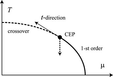
Figure 1: Schematic picture of the QCD phase diagram. CEP is an abbreviation for the critical end point, which is located at $(\mu_{\mathrm{E}},T_{\mathrm{E}})$. The dotted line with an arrow indicates the evolving direction considered in the present analysis.

In the vicinity of CEP located at $(\mu_{\mathrm{E}},T_{\mathrm{E}})$, the critical behaviors are predominantly described by the lightest mode, i.e. the $\sigma$ meson (long-ranged correlation in the scalar-isoscalar-channel) alone. Since the $\sigma$ meson is a scalar particle associated with the Z(2) symmetry, the universality argument tells us that the chiral phase transition belongs to the same universality class as that of the 3-$d$ Ising model. It is worth noting that the chiral restoration at CEP would become a genuine phase transition, namely, a second-ordered phase transition, even though it is a crossover at lower baryon chemical potential. Then singularities around that critical point are characterized by the critical exponents as functions of the distance from the critical point. In general this distance $l$ in the $(\mu,T)$-plane becomes an admixture of both temperature-like (denoted by $t$) and magnetic-like (denoted by $h$) variations in the Ising model: The Z(2) symmetry is only exact right at CEP and the effective potential is distorted away from that point. In the QCD phase diagram the $t$-like direction, along which deformations of the effective potential should preserve the Z(2) symmetry, is tangential to the first-ordered line, as depicted in Fig. 1.

The critical exponents for the 3-$d$ Ising model have been well examined analytically as well as numerically gui97 . The inverse correlation function and the spontaneous magnetization would vanish as $\xi^{-1}\sim t^{\nu}\sim t^{0.63}$ and $m\sim t^{\beta}\sim t^{0.33}$ along the $t$-direction and as $\xi^{-1}\sim h^{\nu/\beta\delta}\sim h^{0.40}$ and $m\sim h^{1/\delta}\sim h^{0.21}$ along the $h$-direction, respectively. It turns out from these numerical values that the magnetic singularities should dominate as long as $l$ contains a non-vanishing component in the $h$-direction, or in other words, they should dominate unless the direction specified by $l$ is parallel to the pure $t$-direction tangential to the first-ordered line. As a result, singularities in almost all directions can be effectively described by the magnetic exponents, as discussed in Ref. ste98 . Then the mass of the $\sigma$ meson, which can be interpreted as the inverse correlation length in the Ising model, vanishes near CEP as $\sim l^{\nu/\beta\delta}$, while the scalar condensate drops off as $\sim l^{1/\delta}$ as though it would be a spontaneous magnetization. The pion mass $m_{\pi}$, on the other hand, can be approximately regarded as constant up to the critical point, which is common in several model studies hat85 ; sca01 ; chi98 .

For simplicity we restrict our discussion throughout this paper only to the case with the chemical potential fixed at $\mu=\mu_{\mathrm{E}}$ (the direction indicated by the dotted line in Fig. 1). In this case, $l$ is proportional to $T-T_{\mathrm{E}}$, and we can parametrize the (screening) masses simply as follows:

$$m_{\pi}(T)=m_{\pi}^{\ast},\quad m_{\sigma}(T)=m_{\sigma}^{\ast}\biggl{\{}1-\biggl{(}\frac{T}{T_{\mathrm{E}}}\biggr{)}^{2}\biggr{\}}^{\nu/\beta\delta},$$ (1)

with $\nu/\beta\delta=0.403$. Also the scalar condensate, that is, the counterpart of the spontaneous magnetization in the Ising model can be parametrized as

$$f_{\pi}(T)=v_{0}+v(T)=af_{\pi}^{\ast}+(1-a)f_{\pi}^{\ast}\biggl{\{}1-\biggl{(}\frac{T}{T_{\mathrm{E}}}\biggr{)}^{2}\biggr{\}}^{1/\delta},$$ (2)

with $1/\delta=0.208$. Here $v_{0}$ is the condensate remaining at CEP due to explicit breaking of the chiral symmetry. It should be noted that the scalar condensate can be regarded as the pion decay constant under some approximations. Accordingly we denote the condensate as $f_{\pi}(T)$ in Eq. (2). Indeed, this identification for the pion decay constant is used in the choice of the parameter sets, as stated below.

The universality argument tells nothing about the values of $m_{\pi}^{\ast}$, $m_{\sigma}^{\ast}$, $f_{\pi}^{\ast}$ (the pion mass, the $\sigma$ mass, and the pion decay constant at $(\mu=\mu_{\mathrm{E}},\>T=0)$ respectively), and $v_{0}$. In the present analysis these are all treated as free parameters, which should be arranged by hand or by using some models. Here, avoiding artifacts inherent in any model study, we simply employ the typical parameter sets as follows, that is, we take two extreme cases, one with no change of the $\ast$-quantities and another with a relatively large change of the $\ast$-quantities:

$$\text{(CASE-I)}\qquad m_{\pi}^{\ast}=140\;\mathrm{MeV},\quad m_{\sigma}^{\ast}=600\;\mathrm{MeV},\quad f_{\pi}^{\ast}=93\;\mathrm{MeV},$$

$$\text{(CASE-II)}\qquad m_{\pi}^{\ast}=140\;\mathrm{MeV},\quad m_{\sigma}^{\ast}=300\;\mathrm{MeV},\quad f_{\pi}^{\ast}=46.5\;\mathrm{MeV}.$$ (3)

As for the choice of $a$, for the moment we will show the results of the spectral functions and the diphoton emission rates only for a specific choice of $a=1/2$; the condensate at CEP decreases up to the half of its value at zero temperature. Finally we will present in Fig. 7 the results for a variety of $a$ ranging from $0.2$ to $0.9$. The qualitative consequences are hardly amended by a change of $a$, though the absolute amount of the diphoton yield depends on $a$.

We should remark that the choice of CASE-II may have a relation to the Brown-Rho scaling hypothesis in dense matter bro91 , i.e. $m_{\sigma}^{\ast}/m_{\sigma}\simeq f_{\pi}^{\ast}/f_{\pi}\simeq\Phi(\rho_{\mathrm{E}})$ where $\rho_{\mathrm{E}}$ is the baryon number density corresponding to the chemical potential $\mu_{\mathrm{E}}$. CASE-II implies the choice of $\Phi(\rho_{\mathrm{E}})=1/2$. Taking into account the fact that the partial restoration of the chiral symmetry might be experimentally observed in nuclei bon96 ; hat99 , we can anticipate that such reduction up to the half may happen in the vicinity of CEP.

III spectral functions near the critical end point

From the experimental point of view, functional forms of the meson masses and the condensate assigned by Eqs. (1) and (2) are not sufficient to describe physical decay processes, that is, the decay width and the amplitude must be evaluated. These informations are contained in the spectral functions. Actually the spectral functions in the $\sigma$-channel are necessary to estimate the diphoton emission rates. Therefore, in this section, we are going to draw our knowledge on the spectral functions in the $\sigma$-channel, limiting our consideration to the case with the spatial momentum fixed at zero. The spectral function in the $\sigma$-channel is defined as

$$\rho_{\sigma}(p)=-\frac{1}{\pi}\mathrm{Im}D_{\sigma}^{\mathrm{R}}(p)=-\frac{1}{\pi}\cdot\frac{\mathrm{Im}\Pi_{\sigma}^{\mathrm{R}}(p)}{(p^{2}-m^{2}-\mathrm{Re}\Pi_{\sigma}^{\mathrm{R}})^{2}+(\mathrm{Im}\Pi_{\sigma}^{\mathrm{R}}(p))^{2}}.$$ (4)

$D_{\sigma}^{\mathrm{R}}(p)$ and $\Pi_{\sigma}^{\mathrm{R}}(p)$ are the retarded Green’s function and the retarded self-energy in the $\sigma$-channel, respectively. In principle, all we have to do is calculate the self-energy $\Pi_{\sigma}^{\mathrm{R}}(p)$ near the critical point as performed, for example, in Ref. chi98 .

In place of performing some resummation procedures, we calculate only the imaginary-part of the self-energy using the propagators with the parametrized masses. One-loop diagrams shown in Fig. 2 describe the decay processes $\sigma\rightarrow 2\sigma$ and $\sigma\rightarrow 2\pi$. We would emphasize that this is not a simple perturbative expansion but rather a resummed calculation since the propagator incorporates the interaction in the mean-field of masses given by $m_{\pi}(T)$ and $m_{\sigma}(T)$. Also the full-vertices represented by boxes in Fig. 2 can be inferred from the effective potential (Appendix A for detail arguments).

Figure 2: Diagrams for the self-energy with non-vanishing imaginary-part up to the one-loop order. Boxes stand for the full-vertices inferred from the effective potential.

Here we limit ourselves to the case in the back-to-back kinematics, that is, diphoton emission with zero spatial momentum. Then we obtain

$$\mathrm{Im}\Pi_{\sigma}^{\mathrm{R}}(\omega,\vec{0})= -\frac{V_{\sigma\sigma\sigma}^{2}}{32\pi}\sqrt{1-\frac{4m_{\sigma}^{2}}{\omega^{2}}}\Bigl{(}1+2n_{\mathrm{B}}(\omega/2)\Bigr{)}\,\theta(\omega-2m_{\sigma})$$

$$\qquad-\frac{3V_{\sigma\pi\pi}^{2}}{32\pi}\sqrt{1-\frac{4m_{\pi}^{2}}{\omega^{2}}}\Bigl{(}1+2n_{\mathrm{B}}(\omega/2)\Bigr{)}\,\theta(\omega-2m_{\pi}),$$ (5)

where $n_{\mathrm{B}}(\omega/2)$ stands for the usual Bose distribution function and $\theta(\omega-2m)$ is the step function. The expressions for the vertices $V_{\sigma\sigma\sigma}$ and $V_{\sigma\pi\pi}$ are given in terms of $m_{\pi}(T)$, $m_{\sigma}(T)$, and $f_{\pi}(T)$ in Eq. (18) in Appendix A.

We have neglected processes involving quark (nucleon) loops such as $\sigma\rightarrow q\bar{q}$ ($\sigma\rightarrow N\bar{N}$) because of physical and technical reasons. First of all, it should be negligible at CEP since the constituent quark is still heavy ($\sim 100\;\mathrm{MeV}$), while the $\sigma$ meson becomes light. Furthermore, the inclusion of quarks needs the wave-function renormalization, in which we cannot avoid technical complications and ambiguities.

It is worth noting that the parametrized mass is the curvature of the effective potential, i.e. the screening mass. The pole mass appearing in the calculation of the self-energy might be different from the parametrized one due to the Lorentz anisotropy at finite temperature and/or density. In Ref. boy02 it is clarified that the anisotropy results in the dynamical critical exponent $z\simeq 1+1/27$ for the $\phi^{4}$-theory slightly above $T_{\mathrm{c}}$ at zero density. The underlying physical contents of massless $\sigma$ mesons near CEP are effectively the same as the critical phenomena described by the $\phi^{4}$-theory. Thus we extrapolate the results of Ref. boy02 and suppose that the effect of the dynamical critical exponent is small enough to be negligible even below $T_{\mathrm{c}}$ at finite density. This presumption of neglecting the dynamical critical exponent formally corresponds to a specific choice of renormalization conditions like the fastest apparent convergence (FAC) condition adopted in Hatree-type resummations chi98 , in which the coupling constant contained in models should depend on the temperature, in principle.

Also we briefly comment upon the results of Ref. sca01 . The authors argued that the pole mass of the $\sigma$ meson within the NJL-model remains finite even right at CEP in the leading order of the $1/N_{\mathrm{c}}$ expansion. This is not because of the treatment of the zero-point energy as discussed by the authors, but because of the lack of infrared dynamics. We have found that the massless $\sigma$ loops dependent on the external momentum are essential ingredients to describe the critical properties fuk01 .

Now that we have the imaginary-part of the self-energy, we can construct the real-part from its imaginary-part via the dispersion relation, i.e.

$$\mathrm{Re}\Pi_{\sigma}^{\mathrm{R}}(\omega,\vec{0})=\frac{1}{\pi}\mathcal{P}\int_{s_{0}}^{\infty}\mathrm{d}s\,\frac{\mathrm{Im}\Pi_{\sigma}^{\mathrm{R}}(\sqrt{s},\vec{0})}{s-\omega^{2}}+\text{(subtractions)},$$ (6)

apart from subtraction factors which are to be determined by the renormalization conditions, in principle. $\mathcal{P}$ stands for the prescription of Cauchy’s principal value. As for the subtractions, meson one-loops need only one subtraction, which is absorbed in the mass-renormalization. We can fix the subtraction factor without ambiguity by demanding the $\sigma$ mass to be given by Eq. (1), neglecting the effect of the dynamical critical exponent. If quark loops were taken into account, they would need two subtractions in the one-loop order, which are absorbed not only in the mass renormalization but in the wave-function renormalization also. This makes the actual computation quite intricate, though the quantitative behaviors are essentially described by meson loops only.

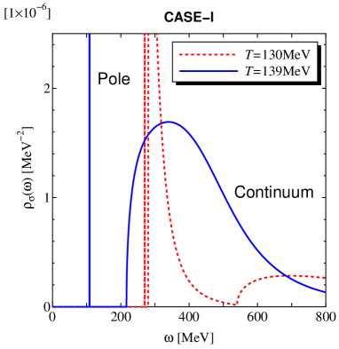
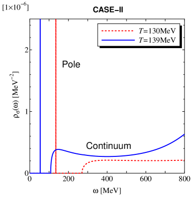
Figure 3: Spectral functions in the $\sigma$-channel near CEP located at $(\mu_{\mathrm{E}}=700\>\mathrm{MeV},T_{\mathrm{E}}=140\>\mathrm{MeV})$. The left figure is for the parameter set of CASE-I ($\Phi(\rho_{\mathrm{E}})=1$) and the right for that of CASE-II ($\Phi(\rho_{\mathrm{E}})=1/2$).

Then we can evaluate the spectral functions in the $\sigma$-channel by substituting $\mathrm{Im}\Pi_{\sigma}^{\mathrm{R}}(\omega)$ and $\mathrm{Re}\Pi_{\sigma}^{\mathrm{R}}(\omega)$ for the definition of Eq. (4). $m^{2}$ in Eq. (4) is irrelevant since it can be absorbed in the subtraction factor. Throughout this analysis we set the location of CEP at $(\mu_{\mathrm{E}}=700\>\mathrm{MeV},\>T_{\mathrm{E}}=140\>\mathrm{MeV})$ as suggested by Refs. ber00 ; fod02 . The resulting spectral functions are shown in Fig. 3 for the cases of $T=130\>\mathrm{MeV}$ and $T=139\>\mathrm{MeV}$. It is clear from the shown spectral functions that the dominant contributions in the low energy region arise from the light $\sigma$ pole and the continuum for the decay process $\sigma\rightarrow 2\sigma$. The threshold of the continuum contribution lies in the point $\omega=2m_{\sigma}(T)$. We note that the process $\sigma\rightarrow 2\pi$ has only slight effects on the spectral function at $T=139\>\mathrm{MeV}$ simply because the full-vertex $V_{\sigma\pi\pi}$ becomes decreasing when the $\sigma$ mass approaches the pion mass, as can be seen in Eq. (18).

To investigate the spectral enhancement in a more quantitative sense, we define the strength of the pole contribution as

$$Z_{\sigma}(\omega)=\frac{1}{2\omega}\biggl{(}1-\frac{\mathrm{d}}{\mathrm{d}\omega^{2}}\Pi_{\sigma}^{\mathrm{R}}(\omega)\biggr{)}^{-1}\biggr{|}_{T=T_{\omega}},$$ (7)

where $T_{\omega}$ is the temperature at which $m_{\sigma}(T=T_{\omega})=\omega$ is satisfied. Then the pole part of the spectral function can be written as $\rho_{\sigma}^{\mathrm{(sing)}}(\omega)=Z_{\sigma}(\omega)\delta(\omega-m_{\sigma}(T))$. In Fig. 4 we plot the strength of the pole contribution as a function of $\omega$. As is clear from the figure, the strength becomes vanishing at $\omega=0$. This property is understood immediately from the dispersion integral of Eq. (6). The differentiation of the integral diverges infraredly ($s\sim 0$) as $\omega\rightarrow 0$. As a result of the infraredly diverging denominator, the spectral function becomes zero at $\omega=0$, which is consistent with the general property of the spectral function $\rho(\omega)=-\rho(\omega)$, for mesons. We will discuss this behavior of the pole strength in connection with the diphoton observation later in Sec. IV.

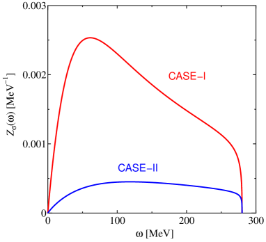
Figure 4: Strength of the pole contributions.

IV the diphoton emission rate

One of the most promising candidates to see the spectral changes in the $\sigma$-channel is the invariant-mass spectrum of diphoton emission from the $\sigma$ meson. The emission rate per unit space-time volume is given by (Appendix B for the derivation) chi98b

$$\frac{\mathrm{d}N}{\mathrm{d}^{4}x\mathrm{d}^{4}p}\biggr{|}_{p=(\omega,\vec{0})}=\frac{|\omega^{2}g_{\sigma\gamma\gamma}(\omega)|^{2}}{(2\pi)^{4}}\cdot\frac{\rho_{\sigma}(\omega,\vec{0})}{\mathrm{e}^{\beta\omega\cosh\theta}-1},$$ (8)

with the effective coupling $g_{\sigma\gamma\gamma}$ of the decay process $\sigma\rightarrow 2\gamma$. Although the expression is proportional to $\omega^{4}$, the singularities in $g_{\sigma\gamma\gamma}(\omega)$ just compensate for $\omega^{4}$ in the presence of a thermal medium and $\omega^{2}g_{\sigma\gamma\gamma}(\omega)$ takes a finite value in the limit of $\omega\rightarrow 0$. The actual evaluation of $g_{\sigma\gamma\gamma}(\omega)$ as a function of $\omega$ is illustrated in Appendix C. $\theta$ is the fluid rapidity related to the fluid velocity $v$ by $\theta=\mathrm{arctanh}v$ arising from the Lorentz boost.

Since they are proportional to each others, the gross features of the multiplicity are the same as those of the spectral function. The dominant contribution, in fact, comes from the $\sigma$ pole when the system lies in a state close to CEP. The results are presented in Fig. 5 for $\theta=0$, in accord with the spectral functions in Fig. 3, respectively.

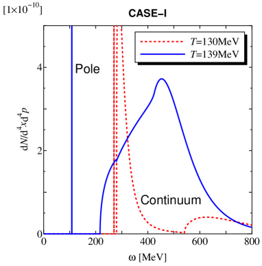
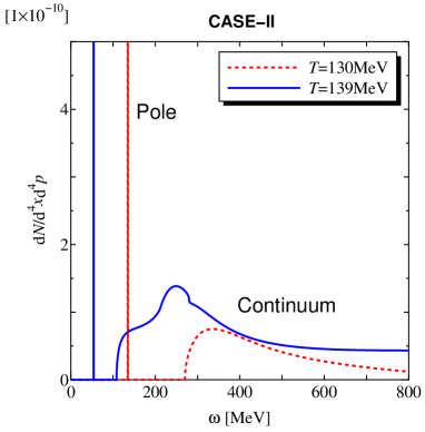
Figure 5: Diphoton emission rates for $\theta=0$. The left figure is for the parameter set of CASE-I ($\Phi(\rho_{\mathrm{E}})=1$) and the right for that of CASE-II ($\Phi(\rho_{\mathrm{E}})=1/2$).

We must take account of the space-time evolution of the system for the calculations to be compared with experimental outputs. Here we adopt the simplest situation for the space-time history, though it is not quantitatively realistic but qualitatively acceptable.

First of all, we fix the baryon chemical potential at $\mu=\mu_{\mathrm{E}}$ during the evolution until freeze-out. This approximation makes the entropy per baryon deviate at most $\sim 10\%$ depending on the nucleon mass around CEP when the equation of state for the ideal gas is used. Considering that neither the nucleon mass nor the equation of state is precisely known around CEP, this approximate path with $\mu=\mu_{\mathrm{E}}$ is the best we can do for the qualitative study.

Secondly, following the analysis presented in Ref. cle87 , we presume that the hydrodynamic evolution would obey the Bjorken’s scaling solution bjo83 . In a quantitative sense the transverse expansion should be taken into account and moreover the boost invariance might be unsatisfied under the experimental conditions where CEP is concerned. Nevertheless, the analysis based on the scaling solution will provide us with the qualitative pattern of the diphoton spectrum when CEP is passed through.

Then the invariant-mass spectrum with the transverse mass $M_{\mathrm{t}}$, the transverse momentum $p_{\mathrm{t}}$ and the momentum rapidity $Y$ of diphotons fixed is given by

$$\frac{1}{\text{(Area)}}\cdot\frac{\mathrm{d}N}{\mathrm{d}M_{\mathrm{t}}^{2}\mathrm{d}^{2}p_{\mathrm{t}}\mathrm{d}Y}\biggr{|}_{p_{\mathrm{t}}=Y=0}=\frac{1}{2}\int_{\tau_{\mathrm{i}}}^{\tau_{\mathrm{f}}}\mathrm{d}\tau\,\tau\int\mathrm{d}y\,\frac{\mathrm{d}N}{\mathrm{d}^{4}x\mathrm{d}^{4}p}\biggr{|}_{p=(M,\vec{0})},$$ (9)

where (Area) is the constant transverse area of the hadronic gas and $y$ is the space-time rapidity which is equal to the fluid rapidity $\theta$ in Bjorken’s scaling solution. $\tau_{\mathrm{i}}$ and $\tau_{\mathrm{f}}$ are the initial and the final time of the evolution; $\tau_{\mathrm{i}}$ is taken as $1\>\mathrm{fm}$ as usual and $\tau_{\mathrm{f}}$ is defined as the time when the system is cooled down below the freeze-out temperature. We fix the freeze-out temperature around CEP as $T_{\mathrm{f}}=120\>\mathrm{MeV}$ according to Ref. ber00 . In order to accomplish the integration with respect to $\tau$, we need the temperature at given $\tau$. That is determined by the following argument, as discussed in Ref. reh97 . Bjorken’s scaling solution leads to the entropy density as a function of time as

$$\frac{s(\tau)}{s(\tau_{\mathrm{i}})}=\frac{\tau_{\mathrm{i}}}{\tau},$$ (10)

from which we can read the temperature once we have a relation connecting the entropy density to the system temperature. For the ideal gases, the entropy density is given by

$$s_{\mathrm{H}}(T)=3\cdot\frac{4\pi^{2}}{90}T^{3}+4\cdot\frac{\partial}{\partial T}\biggl{\{}T\int\frac{\mathrm{d}^{3}k}{(2\pi)^{3}}\Bigl{(}\ln\bigl{[}1+\mathrm{e}^{-\beta(E_{k}-\mu_{\mathrm{E}})}\bigr{]}+\ln\bigl{[}1+\mathrm{e}^{-\beta(E_{k}+\mu_{\mathrm{E}})}\bigr{]}\Bigr{)}\biggr{\}},$$ (11)

for the hadronic gas composed of pions $\pi^{\pm}$, $\pi^{0}$, and nucleons $p$, $n$. Pions can be treated as massless particles, while $E_{k}=\sqrt{k^{2}+M_{\mathrm{n}}^{\ast 2}}$ is the energy of nucleons with the mass $M_{\mathrm{n}}^{\ast}$ in a medium. For the quark-gluon plasma composed of massless gluons and quarks with two flavors $u$, $d$ at quark chemical potential $\mu_{\mathrm{E}}/3$, the entropy density is given by

$$s_{\mathrm{Q}}(T)=\frac{74\pi^{2}}{45}T^{3}+2T\biggl{(}\frac{\mu_{\mathrm{E}}}{3}\biggr{)}^{2}.$$ (12)

In the intermediate temperature we can smoothly interpolate between them as follows:

$$s(T)=\frac{1}{2}\bigl{(}s_{\mathrm{Q}}(T)+s_{\mathrm{H}}(T)\bigr{)}+\frac{1}{2}\bigl{(}s_{\mathrm{Q}}(T)-s_{\mathrm{H}}(T)\bigr{)}\tanh\biggl{(}\frac{T-T_{\mathrm{E}}}{\Delta T}\biggr{)},$$ (13)

where $\Delta T$ controls the strength of the (deconfinement) transition. It is worth noting that the change of the entropy density is mainly attributed to the liberation of the color degrees of freedom and thus it has little to do with the chiral phase transition, at least in principle. There remain subtleties in this respect because no well-defined indicator of confinement is established so far fuk02 . If the deconfinement transition is really related to the chiral dynamics, as often said, the change of the entropy density at CEP (i.e. the terminal point of the first-ordered transition) could be almost discontinuous, that is, $\Delta T$ is small or zero in effect. Here we set $\Delta T=1\>\mathrm{MeV}$.

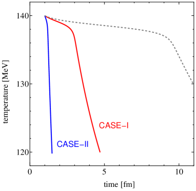
Figure 6: The temperature as a function of time derived from the ansatz given by Eq. (13) with the initial condition $T_{\mathrm{i}}=T_{\mathrm{E}}=140\>\mathrm{MeV}$ at $\tau_{\mathrm{i}}=1\>\mathrm{fm}$.

The temperature as a function of time is shown in Fig. 6 with the initial condition $T_{\mathrm{i}}=T_{\mathrm{E}}=140\>\mathrm{MeV}$ at $\tau_{\mathrm{i}}=1\>\mathrm{fm}$. We take this initial condition, in which the gas is equilibrated right at CEP, for we have parametrized the masses below $T_{\mathrm{E}}$ and have no idea about the masses above CEP. The dotted curve stands for the temperature evolution in the case when the nucleons are infinitely heavy. In CASE-I and CASE-II the nucleon mass $M_{\mathrm{n}}^{\ast}$ is chosen in accord with the Brown-Rho scaling hypothesis, that is, $M_{\mathrm{n}}^{\ast}\simeq 1\>\mathrm{GeV}$ for CASE-I and $M_{\mathrm{n}}^{\ast}\simeq 0.5\>\mathrm{GeV}$ for CASE-II.

We note that the ansatz given by Eq. (13) is implicitly based on a specific choice of the initial entropy density $s(T_{\mathrm{E}})=(s_{\mathrm{H}}(T_{\mathrm{E}})+s_{\mathrm{Q}}(T_{\mathrm{E}}))/2$. The gentle slope of temperature until $\tau\sim 3\>\mathrm{fm}$ ($1.2\>\mathrm{fm}$) in CASE-I (CASE-II) is caused by the difference of the entropy density $s(T_{\mathrm{E}})-s_{\mathrm{H}}(T_{\mathrm{E}})=(s_{\mathrm{Q}}(T_{\mathrm{E}})-s_{\mathrm{H}}(T_{\mathrm{E}}))/2$. Although we will focus our arguments only on the case of the ansatz (13), other forms of interpolation will be necessary when we look into the case with different initial conditions for the entropy density.

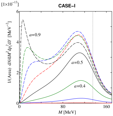
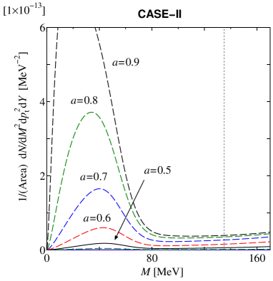
Figure 7: The multiplicity of diphoton emission near CEP. The left figure is for the parameter set of CASE-I ($\Phi(\rho_{\mathrm{E}})=1$) and the right for that of CASE-II ($\Phi(\rho_{\mathrm{E}})=1/2$). The dotted line indicates the position of the pion mass $m_{\pi^{0}}=135\>\mathrm{MeV}$.

Fig. 7 is our final result for the diphoton emission when the system passes through CEP. Because the continuum contribution turns out to be $2\sim 3$ orders of magnitude smaller than the pole contribution, we have plotted only the pole contribution with a variety of $a$ ranging from 0.2 (bottom) to 0.9 (top). We cut the invariant-mass $M$ shown in the figures up to $170\>\mathrm{MeV}$, for the $\sigma$ mass at the freeze-out temperature is around $170\>\mathrm{MeV}$ in CASE-II.

At a glance we notice a characteristic property that the multiplicity approaches zero as $M\rightarrow 0$ and has a peak around $M=50\sim 120\>\mathrm{MeV}$. Although we have expected that the presence of massless $\sigma$ mesons would induce more and more significant enhancement in the multiplicity as $M$ gets smaller and smaller, the resulting multiplicity in the low energy region is reduced altogether. This suppression is because of the amplitude, or the strength of the pole contribution, which is given by Eq. (7).

The location of the peak actually depends on $m_{\sigma}^{\ast}$, $f_{\pi}^{\ast}$ (the $\sigma$ mass and the pion decay constant at $(\mu=\mu_{\mathrm{E}},\>T=0)$), and the evolution of temperature as a function of time. In any case the multiplicity starts from zero at $M=0$. As the energy gets larger, the amplitude rapidly increases and at the same time the space-time volume in which the thermal system stays is reduced by the steeper slope of temperature. Consequently the peak observed in Fig. 7 is produced in somewhat general situations due to the behavior of the amplitude and the time evolution. Thus we can anticipate that the peak found in our analysis appears in different physical conditions (different choices of $m_{\sigma}^{\ast}$, $f_{\pi}^{\ast}$, and the hydrodynamic evolution) as long as the system passes through CEP, though its location is altered according to those conditions.

We would remark that the annihilation process $\pi^{+}\pi^{-}\rightarrow 2\gamma$ makes no background in such a low energy region below the threshold of two pions. In the scenario of the spectral enhancement in the chiral restoration at zero chemical potential, the annihilation process brings about a huge background comparable to the desired signal, which crucially smears the spectral changes chi98 . In contrast, the main background for the CEP peak comes from the electro-magnetic decay into two photons from $\pi^{0}$ in a hot medium and also from $\pi^{0}$ emitted after freeze-out. In the present analysis the pion mass is fixed at a constant value independently of temperature. In addition to the pole contribution at $M=m_{\pi^{0}}=135\>\mathrm{MeV}$, the spectral functions in the pion-channel have a continuum contribution in the low energy region below the pion mass because of the mass difference between pions and $\sigma$ mesons. However, this pion continuum gives rise to so small contribution, which is at most comparable to the continuum contribution in the $\sigma$-channel, that it is sufficiently negligible.

Although the invariant-mass spectrum has a characteristic shape with a peak whose location is separable from the pion pole, the combinatorial background of photons from $\pi^{0}\rightarrow 2\gamma$ will be crucial for experimental observations. The invariant-mass distribution of photon pairs from separate sources is the origin of the combinatorial background. In principle, however, the combinatorial background can be subtracted by means of the event-mixing method. Thus the accuracy necessary to identify the peak originating from $\sigma$ mesons is roughly estimated by the comparison between the number of photons from $\sigma$ mesons and the number of photons from $\pi^{0}$ which might pair with photons from $\sigma$ mesons in the construction of the invariant-mass.

Let us roughly estimate the accuracy necessary to identify the diphoton peak from the $\sigma$ meson in the present formulation, though the analysis should not be reliable beyond a qualitative sense and the quantitative results may be significantly changed under different conditions for the choice of parameters, the initial values of the temperature and the chemical potential, the equation of state, the hydrodynamic evolution, and so on.

The $\pi^{0}$ yield in the present condition can be estimated by the integration of the Bose distribution function on the freeze-out surface as cse98

$$\frac{1}{\text{(Area)}}\frac{\mathrm{d}N_{\pi^{0}}}{\mathrm{d}Y}\simeq\frac{\zeta(3)\tau_{\mathrm{f}}T_{\mathrm{f}}^{3}}{\pi^{2}}\simeq 0.13\>\mathrm{fm}^{-2},$$ (14)

with $\tau_{\mathrm{f}}=4.7\>\mathrm{fm}$ and $T_{\mathrm{f}}=120\>\mathrm{MeV}$ (CASE-I) substituted. This value of the $\pi^{0}$ yield seems small as compared with, for example, the particle production observed in AGS ahl98 . It is because we set the initial point where the system reaches equilibrium right at CEP, not above it. As a result the freeze-out time $\tau_{\mathrm{f}}$ becomes smaller.

Since almost all the $\pi^{0}$ decays via an electro-magnetic process into two photons, the number of photons from $\pi^{0}$ is estimated as twice of Eq. (14). On the other hand, the invariant-mass spectrum of diphoton emission with the range up to $p_{\mathrm{t}}\sim M\sim 100\>\mathrm{MeV}$ integrated out gives

$$\frac{1}{\text{(Area)}}\frac{\mathrm{d}N_{\sigma\gamma\gamma}}{\mathrm{d}Y}\sim 10^{-8}\>\mathrm{fm}^{-2}.$$ (15)

As a rough estimate, the accuracy of order $\sim 10^{-7}$ to the $\pi^{0}$ peak after the subtraction of the combinatorial background is necessary to detect the clear signal from nearly massless $\sigma$ mesons. The infrared suppression of the amplitude we find in the present paper is responsible for the smallness of the resulting output (15). As we stated above, however, the quantitative results here may be considerably changed. For reliable quantitative analyses, we must clarify the hydrodynamic properties around CEP, which are just beginning to be investigated asa02 .

V summary

We investigate the spectral functions in the $\sigma$-channel near CEP where the first-ordered transition of the chiral restoration would terminate. The $\sigma$ pole and the continuum from the decay process $\sigma\rightarrow 2\sigma$ dominate over the spectral functions near CEP, as expected. Our method has almost no model artifact though it contains some parameters put by hand. In the present analysis we try two parameter sets in the extreme cases; one is the case with no medium effect and another is the case with a considerably large medium effect.

Using the resulting spectral functions we have evaluated the multiplicity of diphoton emission. Within the simplest space-time evolution described by Bjorken’s scaling solution, we present the theoretical prediction for the diphoton emission when the system passes through CEP in a hydrodynamic evolution. Our results show that the diphoton multiplicity with vanishing transverse momentum has the characteristic shape with a peak around the invariant mass $50\sim 120\>\mathrm{MeV}$. We find, contrary to expectation, that the infrared dynamics makes the amplitude of nearly massless $\sigma$ mesons so suppressed that the CEP signal is weakened. The severe background comes from a large peak produced by $\pi^{0}$ after freeze-out.

To proceed further and employ more realistic hydrodynamics, it is essential for the present framework to settle the parametrization in the whole $(\mu,T)$-plane and extend it above the critical point. As for the chiral critical point in three flavor QCD at finite temperature gav94 , lattice simulations prove to be powerful instruments to search for the $t$-like and the $h$-like directions kar01 . Unfortunately, however, CEP located at high density is still hard to access by means of lattice simulations.

Appendix A interactions near the critical end point

In the presence of finite chemical potential for the baryon density, the effective potential in terms of $\sigma$ and $\pi$ can be expanded as

$$V(\sigma,\vec{\pi})=A(\sigma^{2}+\vec{\pi}^{2})^{3}-B(\sigma^{2}+\vec{\pi}^{2})^{2}+C(\sigma^{2}+\vec{\pi}^{2})-D\sigma,$$ (16)

where the last term embodies explicit breaking of the chiral symmetry due to finite quark masses. The effects arising from finite chemical potential induce the first term of the sixth power (finite $A$) and reduce the second term of the fourth power (small $B$). As a result the phase transition could be first-ordered. In the vicinity of CEP, coefficients $A$, $B$, $C$, and $D$ are determined by the following conditions: $\partial^{2}V/\partial\pi^{2}=m_{\pi}^{2}$ and $\partial^{2}V/\partial\sigma^{2}=m_{\sigma}^{2}$ for the meson masses given by Eq. (1), $\partial V/\partial\sigma=0$ for the condensation given by Eq. (2), and $\partial^{3}V/\partial\sigma^{3}=0$ for CEP. We need one more condition to determine all the coefficients away from CEP because the last condition is peculiar just to CEP. Then we assume that $A$ can be regarded as constant in our analysis. Actually we can expect that the value of $A$ is more sensitive to $\mu$, which is fixed as $\mu=\mu_{\mathrm{E}}$ throughout this paper, rather than $T$ remembering that $A$ stems from the effects of finite chemical potential. Then it follows that

$$A=\frac{m_{\pi}^{2}}{16v_{0}^{4}},\quad B=\frac{3f_{\pi}^{2}m_{\pi}^{2}}{16v_{0}^{4}}+\frac{m_{\pi}^{2}-m_{\sigma}^{2}}{8f_{\pi}^{2}},\quad C=\frac{3f_{\pi}^{4}m_{\pi}^{2}}{16v_{0}^{4}}+\frac{3m_{\pi}^{2}-m_{\sigma}^{2}}{4},\quad D=f_{\pi}m_{\pi}^{2}.$$ (17)

leading to the full-vertices of the three-point interactions as

$$V_{\sigma\sigma\sigma} \equiv\frac{\partial^{3}V}{\partial\sigma^{3}}=\frac{3f_{\pi}^{3}m_{\pi}^{2}}{v_{0}^{4}}-\frac{3(m_{\pi}^{2}-m_{\sigma}^{2})}{f_{\pi}},$$

$$V_{\sigma\pi\pi} \equiv\frac{\partial^{3}V}{\partial\sigma\partial\pi^{2}}=-\frac{m_{\pi}^{2}-m_{\sigma}^{2}}{f_{\pi}}.$$ (18)

Appendix B formulation of the diphoton emission rate

The multiplicity of two photons (diphotons) per unit space-time volume is given in the thermal circumstance by

$$\frac{\mathrm{d}N}{\mathrm{d}^{4}x}=\sum_{f,i,\lambda_{1},\lambda_{2}}\frac{\mathrm{e}^{-\beta E_{i}}}{Z(\beta)}\cdot\frac{|\langle f;\gamma(k_{1},\lambda_{1})\gamma(k_{2},\lambda_{2})|S|i\rangle|^{2}}{VT}\cdot\frac{\mathrm{d}^{3}k_{1}}{2\omega_{1}(2\pi)^{3}}\cdot\frac{\mathrm{d}^{3}k_{2}}{2\omega_{2}(2\pi)^{3}},$$ (19)

where $Z(\beta)$ is the partition function and the $S$-matrix is denoted by $S$. Two photons have four-momenta $(\omega_{1}=|k_{1}|,\vec{k_{1}})$, $(\omega_{2}=|k_{2}|,\vec{k_{2}})$ and polarization vectors $\epsilon_{\mu}(\lambda_{1})$, $\epsilon_{\mu}(\lambda_{2})$ respectively. The $S$-matrix depends on the actual processes which can be expressed through the effective Lagrangian, i.e.

$$\mathcal{L}_{\phi\gamma\gamma}=g_{\phi\gamma\gamma}\phi F_{\mu\nu}F^{\mu\nu},$$ (20)

with the effective coupling constant $g_{\phi\gamma\gamma}$ of order $\alpha_{\mathrm{e}}\simeq 1/137$. In our notation $\phi$ denotes collectively any particle which can decay into two photons such as $\pi^{0}$ and $\sigma$ mesons. We will focus our attention to the case of $\phi=\sigma$ in the present paper because we are interested in the diphoton spectrum in the low energy region. Up to the lowest order of the perturbation with respect to $g_{\phi\gamma\gamma}$, the $S$-matrix can be expanded as

$$\langle f;\gamma(k_{1},\lambda_{1})\gamma(k_{2},\lambda_{2})|S|i\rangle$$

$$=-4\mathrm{i}g_{\phi\gamma\gamma}\bigl{\{}(k_{1}\cdot k_{2})(\epsilon_{1}^{\ast}\cdot\epsilon_{2}^{\ast})-(k_{1}\cdot\epsilon_{2}^{\ast})(k_{2}\cdot\epsilon_{1}^{\ast})\bigr{\}}\int\mathrm{d}^{4}x\,\mathrm{e}^{\mathrm{i}(k_{1}+k_{2})}\langle f|\hat{\phi}(x)|i\rangle.$$ (21)

Since real (on-shell) photons are emitted, we must take the summation with respect to the polarizations only over the transverse components. The Ward identity, however, simplifies the manipulations, that is, we reach the correct answer simply by taking the summation over all the polarizations. Thus we can make use of the formula, $\sum_{\lambda}\epsilon_{\mu}(\lambda)\epsilon_{\nu}^{\ast}(\lambda)=-g_{\mu\nu}$, to acquire

$$\frac{\mathrm{d}N}{\mathrm{d}^{4}x}=\mathrm{i}D_{\phi}^{<}(k_{1}+k_{2})\cdot 32|g_{\phi\gamma\gamma}|^{2}(k_{1}\cdot k_{2})^{2}\cdot\frac{\mathrm{d}^{3}k_{1}}{2\omega_{1}(2\pi)^{3}}\cdot\frac{\mathrm{d}^{3}k_{2}}{2\omega_{2}(2\pi)^{3}},$$ (22)

after taking the summation over states. Here, the Green’s function,

$$\mathrm{i}D_{\phi}^{<}(p)=\int\mathrm{d}^{4}x\,\mathrm{e}^{\mathrm{i}p\cdot x}\langle\hat{\phi}(0)\hat{\phi}(x)\rangle_{\beta},$$ (23)

can be related to the spectral function as bel96

$$\mathrm{i}D_{\phi}^{<}(p)=\frac{2\pi\rho_{\phi}(p)}{\mathrm{e}^{\beta p_{0}}-1},$$ (24)

where the spectral function is defined as Eq. (4). If the thermal medium has the flow velocity specified by $u_{\mu}$ then $\beta p_{0}$ in the above expression should be replaced by $\beta p\cdot u$.

In the kinematics specified by $\omega_{1}+\omega_{2}=\omega$ and $\vec{p}=\vec{0}$ (back-to-back kinematics), we can easily perform the integration over $\vec{k}_{1}$ and $\vec{k}_{2}$. Taking into account the symmetry factor of identical bosons (photons), we finally reach

$$\frac{\mathrm{d}N}{\mathrm{d}^{4}x\mathrm{d}^{4}p}=\frac{|\omega^{2}g_{\phi\gamma\gamma}(\omega)|^{2}}{(2\pi)^{4}}\cdot\frac{\rho_{\phi}(\omega,\vec{0})}{\mathrm{e}^{\beta\omega}-1}.$$ (25)

Appendix C effective coupling constant

Figure 8: Diagrams contributing the decay process $\sigma\rightarrow 2\gamma$ in the chiral quark model. The box indicates the full vertex of $\sigma\rightarrow 2\pi$ inferred from the effective potential.

The effective coupling constant describing the decay $\sigma\rightarrow 2\gamma$ has been calculated within the framework of the linear sigma model at zero temperature had88 and within the framework of the NJL model at finite temperature reh97 . In the present analysis we estimate the coupling $g_{\sigma\gamma\gamma}$ by means of the chiral quark model at finite baryon density as well as at finite temperature. Diagrams to be calculated are shown in Fig. 8. The result in the back-to-back kinematics is written as

$$g_{\sigma\gamma\gamma}(\omega)=\alpha_{\mathrm{e}}\bigl{(}t_{\pi}^{\text{(vac)}}(\omega)+t_{\pi}^{\text{(mat)}}(\omega)+t_{q}^{\text{(vac)}}(\omega)+t_{q}^{\text{(mat)}}(\omega)\bigr{)},$$ (26)

where $\alpha_{\mathrm{e}}=e^{2}/4\pi$ is the electro-magnetic coupling constant. $t_{\pi}^{\text{(vac)}}$ and $t_{\pi}^{\text{(mat)}}$ represent the vacuum and the medium contributions of the pion loops respectively, given by

$$t_{\pi}^{\text{(vac)}}(\omega) =\frac{V_{\sigma\pi\pi}}{4\pi\omega^{2}}\Biggl{\{}1-\frac{4m_{\pi}^{2}}{\omega^{2}}\biggl{(}\sin^{-1}\frac{\omega}{2m_{\pi}}\biggr{)}^{2}\Biggr{\}},$$

$$t_{\pi}^{\text{(mat)}}(\omega) =\frac{V_{\sigma\pi\pi}m_{\pi}^{2}}{\pi\omega^{2}}\Biggl{\{}\int_{0}^{\infty}\mathrm{d}q\frac{2q\,n_{\mathrm{B}}(E_{q})}{E_{q}^{2}(\omega^{2}-4E_{q}^{2})}\ln\biggl{|}\frac{E_{q}+q}{E_{q}-q}\biggr{|}$$

$$\qquad\qquad-\theta(\omega-2m_{\pi})\,\frac{\mathrm{i}\pi}{\omega^{2}}n_{\mathrm{B}}(\omega/2)\ln\Biggl{|}\frac{\omega+\sqrt{\omega^{2}-4m_{\pi}^{2}}}{\omega-\sqrt{\omega^{2}-4m_{\pi}^{2}}}\Biggr{|}\Biggr{\}},$$ (27)

with the notation $E_{q}=\sqrt{q^{2}+m_{\pi}^{2}}$. The vacuum and the medium contributions, $t_{q}^{\text{(vac)}}$ and $t_{q}^{\text{(mat)}}$ come from the quark loops, which are given by

$$t_{q}^{\text{(vac)}}(\omega) =-\frac{5g\,m_{q}}{3\pi\omega^{2}}\Biggl{\{}1+\biggl{(}1-\frac{4m_{q}^{2}}{\omega^{2}}\biggr{)}\biggl{(}\sin^{-1}\frac{\omega}{2m_{\pi}}\biggr{)}^{2}\Biggr{\}},$$

$$t_{q}^{\text{(mat)}}(\omega) =-\frac{5g\,m_{q}(\omega^{2}-4m_{q}^{2})}{3\pi\omega^{2}}\Biggl{\{}\int_{0}^{\infty}\mathrm{d}q\frac{q(n_{\mathrm{F}}(E_{q}+\mu_{q})+n_{\mathrm{F}}(E_{q}-\mu_{q}))}{E_{q}^{2}(\omega^{2}-4E_{q}^{2})}\ln\biggl{|}\frac{E_{q}+q}{E_{q}-q}\biggr{|}$$

$$\qquad-\theta(\omega-2m_{q})\,\frac{\mathrm{i}\pi}{2\omega^{2}}(n_{\mathrm{F}}(\omega/2+\mu_{q})+n_{\mathrm{F}}(\omega/2-\mu_{q}))\ln\Biggl{|}\frac{\omega+\sqrt{\omega^{2}-4m_{q}^{2}}}{\omega-\sqrt{\omega^{2}-4m_{q}^{2}}}\Biggr{|}\Biggr{\}},$$ (28)

with $E_{q}=\sqrt{q^{2}+m_{q}^{2}}$ as above. $g$ is the strength of the Yukawa-coupling between mesons and quarks. $m_{q}$ denotes the constituent quark mass. We have chosen $g=3.2$ so as to reproduce the constituent quark mass at tree-level, that is, $m_{q}=gf_{\pi}=300\>\mathrm{MeV}$ goc91 .

It is important to note that diagrams in Fig. 8 have no $\sigma$ loop since the $\sigma$ mesons are electrically neutral. Thus it is absolutely necessary to include the contribution from quark loops in contrast to the calculation of the self-energy in which the $\sigma$ contribution dominates over the quark loops.

References

- (1) K. Kanaya, “Recent Lattice Results relevant for Heavy Ion Collisions,” Talk at QM2002, Nantes, 2002, e-print: hep-ph/0209116.
- (2) R.D. Pisarski and F. Wilczek, Phys. Rev. D29, 338 (1984).
- (3) S.P. Klevansky, Rev. Mod. Phys. 64, 649 (1992) and references therein.
- (4) M. Asakawa and K. Yazaki, Nucl. Phys. A504, 668 (1989).
-
(5)
A. Barducci, R. Casalbuoni, S. De Curtis, R. Gatto, and G. Pettini,
Phys. Lett. B231, 463 (1989);
A. Barducci, R. Casalbuoni, and G. Pettini, Phys. Rev. D49, 426 (1994). - (6) J. Berges and K. Rajagopal, Nucl. Phys. B538, 215 (1999).
- (7) M.A. Halasz, A.D. Jackson, R.E. Shrock, M.A. Stephanov, and J.J.M. Verbaarschot, Phys. Rev. D58, 096007 (1998).
-
(8)
M. Stephanov, K. Rajagopal, and E. Shuryak,
Phys. Rev. Lett. 81, 4816 (1998);
M. Stephanov, K. Rajagopal, and E. Shuryak, Phys. Rev. D60, 114028 (1999). - (9) B. Berdnikov and K. Rajagopal, Phys. Rev. D61, 105017 (2000).
- (10) O. Scavenius, Á. Mócsy, I.N. Mishustin, and D.H. Rischke, Phys. Rev. C64, 045202 (2001).
- (11) T. Ikeda, Prog. Theor. Phys. 107, 403 (2002).
- (12) Z. Fodor and S.D. Katz, JHEP03, 014 (2002).
- (13) P. Senger, “The nucleus-nucleus collision research program at the future facility at GSI,” in: HIRSCHEGG2002, Ultrarelativistic Heavy-Ion Collisions, Hirschegg, 2002.
- (14) K. Imai, Nucl. Phys. A691, 451 (2001).
- (15) T. Hatsuda and K. Kunihiro, Phys. Rev. Lett. 55, 158 (1985).
- (16) H.A. Weldon, Phys. Lett. B274, 133 (1992).
- (17) C. Song and V. Koch, Phys. Lett. B404, 1 (1997).
- (18) S. Chiku and T. Hatsuda, Phys. Rev. D58, 076001 (1998).
- (19) S. Chiku, Prog. Theor. Phys. Suppl. 129, 91 (1998).
- (20) M.K. Volkov, E.A. Kuraev, D. Blaschke, G. Roepke, and S.M. Schmidt, Phys. Lett. B424, 235 (1998).
- (21) D. Jido, T. Hatsuda, and T. Kunihiro, Phys. Rev. D63, 011901 (2001).
-
(22)
A. Patkos, Z. Szep, and P. Szepfalusy,
Phys. Lett. B537, 77 (2002);
A. Patkos, Z. Szep, and P. Szepfalusy, e-print: hep-ph/0206040. - (23) R. Guida and J. Zinn-Justin, Nucl. Phys. B489, 626 (1997) and references therein.
- (24) G.E. Brown and M. Rho, Phys. Rev. Lett. 66, 2720 (1991).
-
(25)
F. Bonutti et al. (CHAOS Collaboration),
Phys. Rev. Lett. 77, 603 (1996);
F. Bonutti et al. (CHAOS Collaboration), Nucl. Phys. A677, 213 (2000). -
(26)
T. Hatsuda, T. Kunihiro, and H. Shimizu,
Phys. Rev. Lett. 82, 2840 (1999).
Z. Aouissat, G. Chanfray, P. Schuck, and J. Wambach, Phys. Rev. C61, 012202 (2000).
D. Davesne, Y.J. Zhang, and G. Chanfray, Phys. Rev. C62, 024604 (2000). - (27) D. Boyanovsky and H.J. de Vega, Phys. Rev. D65, 085038 (2002).
- (28) K. Fukushima and K. Ohnishi, “Is the sigma meson really massless at the critical end point?” under completion.
- (29) J. Cleymans, J. Fingberg, and K. Redlich, Phys. Rev. D35, 2153 (1987).
- (30) J.D. Bjorken, Phys. Rev. D27, 140 (1983).
- (31) P. Rehberg, Yu.L. Kalinovsky, and D. Blaschke, Nucl. Phys. A622, 478 (1997).
- (32) K. Fukushima, “Thermodynamic limit of the canonical partition function with respect to the quark number in QCD,” e-print: hep-ph/0204302.
- (33) L. Csernai, Relativistic Heavy Ion Physics (World Scientific, Singapore, 1998).
- (34) C. Nonaka, in private communications.
- (35) E802 Collaboration (L. Ahle et al.), Phys. Rev. C57, R466 (1998).
- (36) S. Gavin, A. Gocksch, and R.D. Pisarski, Phys. Rev. D49, R3079 (1994).
- (37) F. Karsch, E. Laermann, and C. Schmidt, Phys. Lett. B520, 41 (2001).
- (38) M. Le Bellac, Thermal Field Theory (Cambridge University Press, Cambridge, England, 1996).
- (39) S. Hadjitheodoridis and B. Moussallam, Phys. Rev. D37, 1331 (1988).
- (40) A. Gocksch, Phys. Rev. Lett. 67, 1701 (1991).