hep-ph/0209271

ILL-(TH)-02-7

FERMILAB-Pub-02/197-T

Color-flow decomposition of QCD amplitudes

F. Maltoni,¹ K. Paul,¹ T. Stelzer,¹ S. Willenbrock^1,2

¹Department of Physics

University of Illinois at Urbana-Champaign

1110 West Green Street

Urbana, IL  61801

²Theoretical Physics Department

Fermi National Accelerator Laboratory

P. O. Box 500

Batavia, IL  60510

We introduce a new color decomposition for multi-parton amplitudes in QCD, free of fundamental-representation matrices and structure constants. This decomposition has a physical interpretation in terms of the flow of color, which makes it ideal for merging with shower Monte-Carlo programs. The color-flow decomposition allows for very efficient evaluation of amplitudes with many quarks and gluons, many times faster than the standard color decomposition based on fundamental-representation matrices. This will increase the speed of event generators for multi-jet processes, which are the principal backgrounds to signals of new physics at colliders.

1 Introduction

Amplitudes with many external quarks and gluons are important for calculating the cross section for multi-jet production (alone or together with other particles) at the Fermilab Tevatron, CERN Large Hadron Collider, and future $e^{+}e^{-}$ linear colliders. These processes are the major backgrounds to many new-physics signals, so an accurate description of these final states is essential.

Amplitudes involving many quarks and gluons are difficult to calculate, even at tree level. Over the years, techniques have been developed to calculate these multi-parton amplitudes efficiently [1]. One aspect of such techniques is the systematic organization of the $SU(N)$ color algebra. For example, consider the amplitude for $n$ gluons of colors $a_{1},a_{2},\ldots,a_{n}$ ($a_{i}=1,\ldots,N^{2}-1$). At tree level, such an amplitude can be decomposed as [2]

$${\cal M}(ng)=\sum_{P(2,\ldots,n)}{\rm Tr}\,(\lambda^{a_{1}}\lambda^{a_{2}}\cdots\lambda^{a_{n}})\;A(1,2,\ldots,n)\;,$$ (1)

where $\lambda^{a}$ are the fundamental-representation matrices of $SU(N)$, and the sum is over all $(n-1)!$ permutations of $(2,\ldots,n)$. Each trace corresponds to a particular color structure. The factor associated with each color structure, $A$, is called a partial amplitude. It depends on the four-momenta $p_{i}$ and polarization vectors $\epsilon_{i}$ of the $n$ gluons, represented simply by $i$ in the argument of the partial amplitude. These partial amplitudes are far simpler to calculate than the full amplitude, ${\cal M}$, and they are also gauge invariant. There exist linear relations amongst the partial amplitudes, called Kleiss-Kuijf relations, which reduce the number of linearly-independent partial amplitudes to $(n-2)!$ [3]. A similar decomposition exists for amplitudes containing any number of $\bar{q}q$ pairs and gluons.

Recently, another decomposition of the multi-gluon amplitude has been introduced, based on the adjoint representation of $SU(N)$ rather than the fundamental representation [4, 5]. The $n$-gluon amplitude in this decomposition may be written as

$${\cal M}(ng)=\sum_{P(2,\ldots,n-1)}(F^{a_{2}}F^{a_{3}}\cdots F^{a_{n-1}})^{a_{1}}_{a_{n}}\;A(1,2,\ldots,n)\;,$$ (2)

where $(F^{a})^{b}_{c}=-if^{abc}$ are the adjoint-representation matrices of $SU(N)$ ($f^{abc}$ are the structure constants), and the sum is over all $(n-2)!$ permutations of $(2,\ldots,n-1)$. The partial amplitudes that appear in this decomposition are the same as in the other decomposition, but only the $(n-2)!$ linearly-independent amplitudes are needed. The adjoint-representation decomposition exists only for the multi-gluon amplitude.

In this paper we introduce a third color decomposition of multi-parton amplitudes. This decomposition is based on treating the $SU(N)$ gluon field as an $N\times N$ matrix $(A_{\mu})^{i}_{j}$ ($i,j=1,\ldots,N$), rather than as a one-index field $A_{\mu}^{a}$ ($a=1,\ldots,N^{2}-1$). The $n$-gluon amplitude may be decomposed as

$${\cal M}(ng)=\sum_{P(2,\ldots,n)}\delta^{i_{1}}_{j_{2}}\delta^{i_{2}}_{j_{3}}\cdots\delta^{i_{n}}_{j_{1}}\;A(1,2,\ldots,n)\;,$$ (3)

where the sum is over all $(n-1)!$ permutations of $(2,\ldots,n)$. We dub this the color-flow decomposition, due to its physical interpretation. The partial amplitudes that appear in this decomposition are the same as in the other two decompositions. The proof of this assertion is contained in an Appendix.

The color-flow decomposition has several nice features which we elaborate upon in this paper. First, a similar decomposition exists for all multi-parton amplitudes, like the fundamental-representation decomposition. Second, the color-flow decomposition allows for a very efficient calculation of multi-parton amplitudes. For example, we show that the amplitude for 12 gluons ($gg\to 10g$) may be calculated about 60 times faster using the color-flow decomposition than using the fundamental-representation decomposition. Third, it is a very natural way to decompose a QCD amplitude. As the name suggests, it is based on the flow of color, so the decomposition has a simple physical interpretation. This is also useful for merging the hard-scattering cross section with shower Monte-Carlo programs.

The remainder of the paper is organized as follows. In Section 2 we derive the color-flow Feynman rules for the construction of the partial amplitudes. Section 3 is devoted to the all-gluon amplitude. In Section 4 we consider the amplitude for a $\bar{q}q$ pair and any number of gluons. Section 5 deals with the case of two $\bar{q}q$ pairs and any number of gluons. The general case is discussed in Section 6. We draw conclusions in Section 7.

2 Feynman rules

Consider the Lagrangian of an $SU(N)$ gauge theory,

$${\cal L}=\frac{1}{2g^{2}}{\rm Tr}\,{F^{\mu\nu}F_{\mu\nu}}+\bar{\psi}(i\not\!\!D-m)\psi\;,$$ (4)

where

$$D_{\mu} = \partial_{\mu}+igA_{\mu}$$ (5)

$$F_{\mu\nu} = [D_{\mu},D_{\nu}]\;.$$ (6)

The quark field transforms under the fundamental representation of $SU(N)$,

$$\psi\to U\psi\;.$$ (7)

The gluon field $A_{\mu}$ transforms under the adjoint representation,

$$A_{\mu}\to UA_{\mu}U^{{\dagger}}+\frac{i}{g}(\partial_{\mu}U)U^{{\dagger}}\;,$$ (8)

such that the Lagrangian is invariant under local $SU(N)$ transformations, $U(x)$.

It is conventional to decompose the gluon field using the fundamental-representation matrices,

$$(A_{\mu})^{i}_{j}=\frac{1}{\sqrt{2}}A_{\mu}^{a}(\lambda^{a})^{i}_{j}\;,$$ (9)

and to rewrite the Lagrangian in terms of $A_{\mu}^{a}$ ($a=1,\ldots,N^{2}-1$). This yields the usual Feynman rules involving the fundamental-representation matrices $\lambda^{a}$ and the structure constants $f^{abc}$, which arise from the commutation relation $[\lambda^{a},\lambda^{b}]=if^{abc}\lambda^{c}$. The decomposition of the $n$-gluon amplitude in terms of traces of fundamental-representation matrices, Eq. (1), is then achieved by inverting the commutation relation, $f^{abc}=-i{\rm Tr}\,(\lambda^{a}\lambda^{b}\lambda^{c}-\lambda^{a}\lambda^{c}\lambda^{b})$.

However, it is not necessary to decompose the gluon field $(A_{\mu})^{i}_{j}$ in terms of fundamental-representation matrices. Instead, one can work directly with the $N\times N$ matrix field $({\cal A}_{\mu})^{i}_{j}\equiv\sqrt{2}(A_{\mu})^{i}_{j}$. The Lagrangian is

$${\cal L}=-\frac{1}{4}({\cal F}^{\mu\nu})^{i}_{j}({\cal F}_{\mu\nu})^{j}_{i}+i\bar{\psi}_{i}\gamma^{\mu}(\delta^{i}_{j}\partial_{\mu}+i\frac{g}{\sqrt{2}}({\cal A}_{\mu})^{i}_{j})\psi^{j}-m\bar{\psi}_{i}\psi^{i}\;,$$ (10)

where

$$({\cal F}_{\mu\nu})^{i}_{j}=\partial_{\mu}({\cal A}_{\nu})^{i}_{j}-\partial_{\nu}({\cal A}_{\mu})^{i}_{j}+i\frac{g}{\sqrt{2}}({\cal A}_{\mu})^{i}_{k}({\cal A}_{\nu})^{k}_{j}-i\frac{g}{\sqrt{2}}({\cal A}_{\nu})^{i}_{k}({\cal A}_{\mu})^{k}_{j}\;.$$ (11)

This yields Feynman rules free of fundamental-representation matrices and structure constants. These Feynman rules are given in Fig. 1. This representation of an $SU(N)$ gauge theory is well known from the $1/N$ expansion [7]. However, it is not commonly used for ordinary calculations in QCD.

In our conventions, upper indices transform under the fundamental representation of $SU(N)$, lower indices under the antifundamental representation. Global $SU(N)$ symmetry implies that color is conserved at the interaction vertices, just as electric charge is conserved at the interaction vertex of QED. Thus the interaction vertices may be represented by color-flow Feynman rules, as shown in Fig. 1 [8]. The arrows track the flow of color from lower indices to upper indices. The three-gluon vertex has two color flows, and the four-gluon vertex has six.

The gluon propagator is proportional to

$$\langle({\cal A}_{\mu})^{i_{1}}_{j_{1}}({\cal A}_{\nu})^{i_{2}}_{j_{2}}\rangle\propto\delta^{i_{1}}_{j_{2}}\delta^{i_{2}}_{j_{1}}-\frac{1}{N}\delta^{i_{1}}_{j_{1}}\delta^{i_{2}}_{j_{2}}$$ (12)

and thus has two different color flows. In contrast, the gluon propagator in the conventional representation of color is proportional to

$$\langle A_{\mu}^{a}A_{\nu}^{b}\rangle\propto\delta^{ab}\;.$$ (13)

The more complicated color structure of the gluon propagator is a trade-off for the simplicity of the color structure of the interaction vertices (Fig. 1). As we shall see, this trade-off is worthwhile.

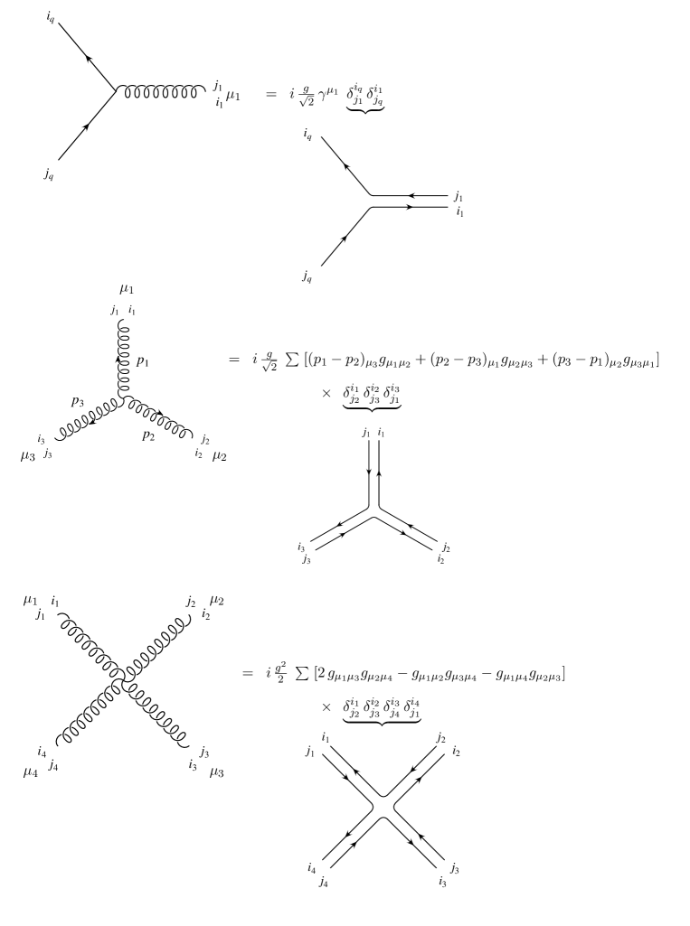
Figure 1: Color-flow Feynman rules. All momenta are outgoing. The arrows indicate the flow of color. The sum in the three-gluon vertex is over the two non-cyclic permutations of (1,2,3); in the four-gluon vertex, the sum is over the six non-cyclic permutations of (1,2,3,4). When calculating a partial amplitude the sum is dropped, as only one term in the sum contributes to a given color flow.

Due to the antisymmetry of the three- and four-gluon vertices, the second color flow in the gluon propagator does not couple to these interactions. It couples only to the gluon interaction with the quarks. This color flow acts as a “photon” that couples with strength $\frac{g}{\sqrt{2}}$ to quarks. We indicate this by splitting the gluon propagator into a $U(N)$ gluon propagator and a $U(1)$ gluon propagator, as shown in Fig. 2. The $U(1)$ gluon is unphysical, as evidenced by its ghostly residue, which also carries a factor $1/N$.

Figure 2: The $SU(N)$ gluon propagator may be split into a $U(N)$ gluon propagator and a $U(1)$ gluon propagator. The $U(1)$ gluon interacts only with quarks.

3 $n$-gluon amplitude

The $n$-gluon tree-level amplitude is constructed from three- and four-gluon vertices and the $U(N)$ gluon propagator; the $U(1)$ gluon propagator does not couple to these interactions. It follows directly from the color-flow Feynman rules that the $n$-gluon tree-level amplitude has the decomposition given in Eq. (3). We now describe how to calculate the partial amplitude, which is the factor associated with a particular color flow.

Figure 3: Color flow $\delta^{i_{1}}_{j_{2}}\delta^{i_{2}}_{j_{3}}\cdots\delta^{i_{n}}_{j_{1}}$. Each pair of indices $i_{k},j_{k}$ corresponds to an external gluon.

To calculate $A(1,2,\ldots,n)$, one orders the gluons clockwise, as shown in Fig. 3, and draws color-flow lines, with color flowing counter-clockwise, connecting adjacent gluons. One then deforms the color-flow lines in all possible ways to form the Feynman diagrams that contribute to this partial amplitude. An example of a four-gluon partial amplitude is given in Fig. 4. At each vertex, one needs only a single color flow in the three- and four-gluon Feynman rules given in Fig. 1. Thus, when constructing a partial amplitude, the sum over permutations in the three- and four-gluon vertices may be dropped.

Figure 4: Feynman diagrams corresponding to a four-gluon partial amplitude.

It is evident that the Feynman diagrams that contribute to a partial amplitude are planar. This is not due to an expansion in $1/N$; the partial amplitudes are exact. The number of Feynman diagrams that contribute to an $n$-gluon partial amplitude is listed in Table 1. The number grows approximately like $3.8^{n}$, rather than the factorial growth of the number of Feynman diagrams that contribute to the full amplitude, approximately $(2n)!$.

Table 1: Number of Feynman diagrams contributing to an $n$-gluon partial amplitude. The number grows approximately like $3.8^{n}$. In contrast, the number of Feynman diagrams contributing to the full amplitude grows factorially, approximately $(2n)!$.

	# diagrams
$n$	partial amplitude	full amplitude
4	3	4
5	10	25
6	36	220
7	133	2485
8	501	34300
9	1991	559405
10	7335	10525900
11	28199	224449225
12	108281	5348843500

This procedure is analogous to the “color-ordered” Feynman rules that have been developed for the fundamental-representation decomposition of multi-gluon amplitudes, Eq. (1) [1, 2]. The similarity of this procedure with the construction of string amplitudes has been noted. Each gluon corresponds to an open string with color-anticolor charges $i,j$ on its ends. The diagram in Fig. 3 represents the scattering of $n$ open strings. The Feynman diagrams in Fig. 4 correspond to the zero-slope limit of the scattering of four open strings [1, 2].

One obtains the cross section from the $n$-gluon amplitude by squaring and summing over the colors of the external gluons. Since each external gluon has two indices, naively summing counts $N^{2}$ colors per gluon. To sum over only the $N^{2}-1$ desired colors, it is sufficient to first apply the projection operator

$$P^{ii^{\prime}}_{jj^{\prime}}\equiv\delta^{i}_{j^{\prime}}\delta^{i^{\prime}}_{j}-\frac{1}{N}\delta^{i}_{j}\delta^{i^{\prime}}_{j^{\prime}}$$ (14)

to each external gluon before squaring and summing over colors. However, the second term in the projection operator corresponds to a $U(1)$ gluon, so it does not couple to the $n$-gluon amplitude. Hence, in the case of the $n$-gluon amplitude, it is sufficient to naively sum over colors. This is not the case if external quarks are present, as we discuss in the following section.

When squaring the amplitude and summing over colors, the leading term in $1/N$ is given by the square of each color flow:

$$\delta^{i_{1}}_{j_{2}}\delta^{i_{2}}_{j_{3}}\cdots\delta^{i_{n}}_{j_{1}}(\delta^{i_{1}}_{j_{2}}\delta^{i_{2}}_{j_{3}}\cdots\delta^{i_{n}}_{j_{1}})^{{\dagger}}=\delta^{i_{1}}_{j_{2}}\delta^{i_{2}}_{j_{3}}\cdots\delta^{i_{n}}_{j_{1}}(\delta^{j_{2}}_{i_{1}}\delta^{j_{3}}_{i_{2}}\cdots\delta^{j_{1}}_{i_{n}})=N^{n}.$$ (15)

Cross terms between different color flows yield monomials $N^{n-m}$, where $m$ is even. This contrasts with the squaring and summing over colors in the fundamental-representation decomposition, Eq. (1). There, each term obtained is a polynomial in $N$, rather than a monomial [1]. In this sense, squaring and summing over colors is simpler in the color-flow decomposition, Eq. (3).

For processes with many external gluons, it is necessary to sum over colors using Monte-Carlo techniques in order to produce a cross section with sufficient speed to be useful in practice [10, 11, 12, 13]. The color-flow decomposition is well suited for such a calculation. One chooses, via Monte-Carlo methods, a particular color assignment for the external gluons. This is accomplished by randomly selecting the colors of the upper and lower indices. A necessary (but not sufficient) condition for a nonvanishing color assignment (one which has at least one color flow) is that the number of upper and lower indices of the color $R$ must be the same; similarly for the colors $G$ and $B$. In general, only a small fraction of the $(n-1)!$ color flows contribute to a given color assignment, so it is necessary to evaluate only a small subset of the partial amplitudes. This is crucial, as most of the computational time is spent on calculating the partial amplitudes. We give in the third column of Table 2 the average number of partial amplitudes that contribute to a given nonvanishing color assignment. Although this number grows factorially with the number of gluons, it grows approximately as $(n/3)!$ rather than $(2n)!$.

Table 2: Average number of partial amplitudes, for $n$-gluon scattering, that must be evaluated per nonvanishing color assignment in three different color decompositions: the fundamental-representation decomposition (using both the Gell-Mann matrices and the matrices used in Ref. [10]), the color-flow decomposition, and the adjoint-representation decomposition. The fundamental-representation decomposition is much more efficient using the matrices of Ref. [10]. The color-flow decomposition is much more efficient than the fundamental-representation decomposition, especially when $n$ is large. The adjoint-representation decomposition is almost as efficient as the color-flow decomposition, but requires the multiplication of sparse $9\times 9$ matrices.

	Decomposition
	Fundamental
$n$	Gell-Mann	Ref. [10]	Color-flow	Adjoint
4	4.83	3.02	1.28	1.15
5	15.2	7.26	1.83	1.52
6	56.5	20.6	3.21	2.55
7	251	68.0	6.80	5.53
8	1280	254	17.0	15.8
9	7440	1080	48.7	56.4
10	47800	4930	158	243
11	337000	25500	570	1210
12	2590000	148000	2250	6750

We have written a code to identify the color flows that contribute to a given color assignment. Once the color flows are identified, one must evaluate the corresponding partial amplitudes. The amplitude for a given color assignment is the sum of these partial amplitudes, with unit coefficients, as per Eq. (3). No matrix multiplication is necessary to evaluate the color coefficients.

Let us compare the efficiency of this procedure with that of the fundamental-representation decomposition, Eq. (1). First we use the standard Gell-Mann matrices (see the Appendix of Ref. [14]) to evaluate the color coefficients. The average number of partial amplitudes that must be evaluated per nonvanishing color assignment is given in the first column of Table 2. It is evident that the fundamental-representation decomposition using the Gell-Mann basis is far less efficient than the color-flow decomposition.

In Ref. [10] a particular basis for the fundamental-representation matrices is chosen in order to minimize the average number of traces of matrices that contribute to a given nonvanishing color assignment. That basis is

$$\lambda^{1}=\frac{1}{\sqrt{2}}\left(\begin{array}[]{ccc}0&1&0\\ 0&0&0\\ 0&0&0\end{array}\right)\quad,\quad\lambda^{2}=\frac{1}{\sqrt{2}}\left(\begin{array}[]{ccc}0&0&1\\ 0&0&0\\ 0&0&0\end{array}\right)\quad,\quad\lambda^{3}=\frac{1}{\sqrt{2}}\left(\begin{array}[]{ccc}0&0&0\\ 1&0&0\\ 0&0&0\end{array}\right)\quad,$$ (25)

$$\lambda^{5}=\frac{1}{\sqrt{2}}\left(\begin{array}[]{ccc}0&0&0\\ 0&0&1\\ 0&0&0\end{array}\right)\quad,\quad\lambda^{6}=\frac{1}{\sqrt{2}}\left(\begin{array}[]{ccc}0&0&0\\ 0&0&0\\ 1&0&0\end{array}\right)\quad,\quad\lambda^{7}=\frac{1}{\sqrt{2}}\left(\begin{array}[]{ccc}0&0&0\\ 0&0&0\\ 0&1&0\end{array}\right)\quad,$$ (35)

$$\lambda^{4}=\frac{1}{{2}}\left(\begin{array}[]{ccc}1&0&0\\ 0&-1&0\\ 0&0&0\end{array}\right)\quad,\quad\lambda^{8}=\frac{1}{\sqrt{12}}\left(\begin{array}[]{ccc}1&0&0\\ 0&1&0\\ 0&0&-2\end{array}\right)\quad.$$ (42)

Using this basis, we give in the second column of Table 2 the average number of partial amplitudes that contribute to a given nonvanishing color assignment. Although much less than the results using the Gell-Mann basis, these numbers are significantly greater than in the color-flow decomposition, especially when $n$ is large. Hence the color-flow decomposition is much more efficient than the fundamental-representation decomposition.

The reason the fundamental-representation decomposition of Ref. [10] is less efficient for evaluating color coefficients is due to the matrices $\lambda^{4}$ and $\lambda^{8}$ above, which have more than one nonvanishing element, and may therefore appear in many traces. To avoid this, it is advantageous to replace these two matrices with the three matrices

$$\lambda^{4}=\frac{1}{\sqrt{2}}\left(\begin{array}[]{ccc}1&0&0\\ 0&0&0\\ 0&0&0\end{array}\right)\quad,\quad\lambda^{8}=\frac{1}{\sqrt{2}}\left(\begin{array}[]{ccc}0&0&0\\ 0&1&0\\ 0&0&0\end{array}\right)\quad,\quad\lambda^{9}=\frac{1}{\sqrt{2}}\left(\begin{array}[]{ccc}0&0&0\\ 0&0&0\\ 0&0&1\end{array}\right)\quad,$$ (52)

thereby expanding to the fundamental representation of $U(3)$. In so doing, one is including the $U(1)$ gluon; however, we know that this gluon decouples from the $n$-gluon tree amplitude, so no error is being made. Using this expanded basis of fundamental-representation matrices is equivalent to the color-flow decomposition, Eq. (3), because each matrix is proportional to a product of Kronecker deltas ($(\lambda^{1})^{i}_{j}=\delta^{i}_{1}\delta^{2}_{j}/\sqrt{2}$, $(\lambda^{2})^{i}_{j}=\delta^{i}_{1}\delta^{3}_{j}/\sqrt{2}$, etc.). However, the color-flow decomposition leads to a faster evaluation of the color coefficients, since no matrix multiplication is necessary, while the multiplication of sparse $3\times 3$ matrices is required in the fundamental-representation decomposition.

Another method for Monte-Carlo summation over color is used in Ref. [12]. Although the fundamental-representation decomposition is used, it is converted to the color-flow decomposition before the summation over color is performed. This is achieved via

$$f^{a_{1}a_{2}a_{3}}(\lambda^{a_{1}})^{i_{1}}_{j_{1}}(\lambda^{a_{2}})^{i_{2}}_{j_{2}}(\lambda^{a_{3}})^{i_{3}}_{j_{3}}=-i(\delta^{i_{1}}_{j_{2}}\delta^{i_{2}}_{j_{3}}\delta^{i_{3}}_{j_{1}}-\delta^{i_{1}}_{j_{3}}\delta^{i_{3}}_{j_{2}}\delta^{i_{2}}_{j_{1}})\;.$$ (53)

This paper goes on to promote color from a discrete to a continuous variable, and performs a Monte-Carlo integration over color. It is not clear that anything is gained by making color a continuous variable, since a Monte-Carlo summation over color is already possible when color is a discrete variable.

We next consider the summation over color in the adjoint-representation decomposition, Eq. (2). This decomposition uses only the $(n-2)!$ linearly-independent partial amplitudes, so it is potentially more efficient than the color-flow decomposition. Rather than using the standard $SU(3)$ structure constants based on the Gell-Mann matrices (see the Appendix of Ref. [14]), we use a set based on the nine $U(3)$ fundamental-representation matrices above, again exploiting the fact that the $U(1)$ gluon decouples. The structure constants in this basis are antisymmetric in the first two indices only, and are given by ($[\lambda^{a},\lambda^{b}]=if^{abc}\lambda^{c}$)

$$f^{314}=f^{138}=f^{512}=f^{167}=f^{141}=f^{811}=f^{235}=f^{624}=f^{269}=f^{721}=f^{242}=f^{922}=f^{376}$$

$$=f^{433}=f^{383}=f^{653}=f^{758}=f^{579}=f^{585}=f^{955}=f^{466}=f^{696}=f^{877}=f^{797}=i/\sqrt{2}\;,$$

where all other structure constants, not related to the above by interchange of the first two indices, vanish. This set of structure constants leads to a much faster evaluation of the color coefficients in Eq. (2) than the standard set of structure constants based on the Gell-Mann matrices. For $n$-gluon scattering, the average number of partial amplitudes that must be evaluated per nonvanishing color assignment is given in the fourth column of Table 2. It is comparable in efficiency to the color-flow decomposition. However, the color-flow decomposition leads to a much faster evaluation of the color coefficients, since the multiplication of sparse $9\times 9$ matrices is required in the adjoint-representation decomposition.

To demonstrate the utility of the color-flow decomposition, we calculate the subprocess cross sections with 11 and 12 external gluons at tree level ($gg\to 9g$ and $gg\to 10g$), results that have not yet appeared in the literature. We employ the same cuts as Ref. [10],

$$p_{Ti}>60\;{\rm GeV}\;,\;\;|\eta_{i}|<2\;,\;\;\Delta R_{ij}>0.7\;,$$ (54)

where the subprocess cross section with 10 external gluons ($gg\to 8g$) at $\sqrt{\hat{s}}=1500$ GeV was presented, using $\alpha_{S}=0.12$ for illustrative purposes. We use the Berends-Giele recursion relations [15] to obtain the partial amplitudes, and evaluate the basic currents upon which these relations are based using HELAS [16]. We increase the subprocess energy for $n=11,12$ to $\sqrt{\hat{s}}=2000,2500$ GeV, respectively, to maintain a roughly constant fraction of generated events that pass the cuts. No effort is made to optimize the generation of the phase space; our goal is to show that the use of the color-flow decomposition speeds up the calculation so much (a factor of about 40 for $n=11$ and about $60$ for $n=12$, see Table 2) that one can obtain the $gg\to 9g$ and $gg\to 10g$ subprocess cross sections with a straightforward phase-space generator such as RAMBO [17]. Using this procedure, we confirm the $n=10$ result of Ref. [10], and give the $n=11,12$ results in Table 3.

Table 3: Subprocess cross section (pb) for $gg\to(n-2)g$ at subprocess energy $\sqrt{\hat{s}}$ (GeV).

$n$	$\sqrt{\hat{s}}$ (GeV)	$\hat{\sigma}(gg\to(n-2)g)$ (pb)
10	1500	$0.70\pm 0.04$
11	2000	$0.30\pm 0.02$
12	2500	$0.097\pm 0.006$

The color-flow decomposition nicely lends itself to merging with a shower Monte Carlo, such as HERWIG [18, 19] or Pythia [20], which is based on the color flow of a given hard-scattering subprocess. A given color assignment typically has several color flows that contribute. One of these color flows is randomly chosen to be associated with the event, weighted by the square of the partial amplitude corresponding to that color flow. The weight does not include a color coefficient (since it is unity), unlike the fundamental-representation decomposition [10]. The event is then evolved with a shower Monte Carlo. This neglects the interference between different color flows, but this interference is suppressed by a power of $1/N^{2}$. This is not a deficiency of the color-flow decomposition, but rather is an inherent feature of the shower Monte-Carlo approximation for soft radiation [21].

4 $\bar{q}q$ and $n$ gluons

Figure 5: The color flow $\delta^{i_{q}}_{j_{1}}\delta^{i_{1}}_{j_{2}}\cdots\delta^{i_{n}}_{j_{q}}$ for one $\bar{q}q$ pair and $n$ gluons.

Consider the case where there is one quark line and $n$ gluons. The outgoing quark has color $i_{q}$, the outgoing antiquark has anticolor $j_{q}$. The color flow is identical to that of the $n$-gluon case, except the $\bar{q}q$ replaces one of the gluons, as shown in Fig. 5. The color-flow decomposition is

$${\cal M}(\bar{q}q+ng)=\sum_{P(1,\ldots,n)}\delta^{i_{q}}_{j_{1}}\delta^{i_{1}}_{j_{2}}\cdots\delta^{i_{n}}_{j_{q}}\;A(q,1,2,\ldots,n,\bar{q})\;,$$ (55)

where the sum is over all $n!$ permutations of $(1,\ldots,n)$. The arguments $q$, $\bar{q}$ in the partial amplitude represent the momenta and helicities of the outgoing quark and antiquark. This decomposition follows directly from the Feynman rules of Figs. 1 and 2 and is similar to the decomposition of the $n$-gluon amplitude. The $U(1)$ gluon propagator, which couples only to quarks, does not contribute at tree level since there is only one quark line. As an example, the Feynman diagrams contributing to a particular partial amplitude for the case of one $\bar{q}q$ and two gluons are shown in Fig. 6.

Figure 6: Feynman diagrams corresponding to a partial amplitude for one $\bar{q}q$ pair and two gluons.

Before squaring the amplitude and summing over colors, one must apply the projection operator, Eq. (14), to each external gluon. This generates terms proportional to powers of $(-1/N)$. In the $n$-gluon case, these terms vanish. In the present case, they do not vanish due to the presence of a quark line to which the external $U(1)$ gluon couples. One obtains

$$P\cdots P{\cal M}(\bar{q}q+ng) = \sum_{P(1,\ldots,n)}\delta^{i_{q}}_{j_{1}}\delta^{i_{1}}_{j_{2}}\cdots\delta^{i_{n}}_{j_{q}}\;A(q,1,2,\ldots,n,\bar{q})$$ (56)

$$+ \left(-\frac{1}{N}\right)\sum_{P(1,\ldots,n)}\delta^{i_{q}}_{j_{1}}\delta^{i_{1}}_{j_{2}}\cdots\delta^{i_{n-1}}_{j_{q}}\delta^{i_{n}}_{j_{n}}\;A(q,1,2,\ldots,n-1,\bar{q},n)$$

$$+ \left(-\frac{1}{N}\right)^{2}\frac{1}{2!}\sum_{P(1,\ldots,n)}\delta^{i_{q}}_{j_{1}}\delta^{i_{1}}_{j_{2}}\cdots\delta^{i_{n-2}}_{j_{q}}\delta^{i_{n-1}}_{j_{n-1}}\delta^{i_{n}}_{j_{n}}\;A(q,1,2,\ldots,n-2,\bar{q},n-1,n)$$

$$\vdots$$

$$+ \left(-\frac{1}{N}\right)^{n}\delta^{i_{q}}_{j_{q}}\delta^{i_{1}}_{j_{1}}\cdots\delta^{i_{n}}_{j_{n}}\;A(q,\bar{q},1,2,\ldots,n)\;,$$

where the partial amplitudes of the subleading terms in $1/N$ are linear combinations of the leading partial amplitudes $A(q,1,2,\ldots,n,\bar{q})$. The subleading partial amplitude $A(q,1,\ldots,n-k,\bar{q},n-k+1,\ldots,n)$ corresponds to the amplitude for $n-k$ gluons and $k$ $U(1)$ gluons. For example, the subleading partial amplitude for one $U(1)$ gluon is given by the linear combination

$$A(q,1,2,\ldots,\bar{q},n)=A(q,1,2,\ldots,n,\bar{q})+A(q,1,2,\ldots,n,n-1,\bar{q})+\cdots+A(q,n,1,2,\ldots,\bar{q})\;.$$ (57)

This is analogous to the photon-decoupling equation for the $n$-gluon amplitude [1, 2, 22],

$$0=A(1,2,\ldots,n)+A(1,2,\ldots,n,n-1)+\cdots+A(1,n,2,\ldots,n-1)\;.$$ (58)

More generally, the linear relations for the subleading partial amplitudes with $k$ $U(1)$ gluons in terms of the leading partial amplitudes are analogous to the Kleiss-Kuijf relations amongst the multi-gluon amplitudes [3].

The sum over permutations of the subleading terms with $k$ $U(1)$ gluons contains a factor $1/k!$, because terms that differ only by the exchange of $U(1)$ gluons are identical. Thus there are $n!/k!$ different permutations in the terms with $k$ $U(1)$ gluons. There is only a single term in which all gluons are $U(1)$, given at the end of Eq. (56).

It is more efficient to calculate the subleading partial amplitudes directly, rather than as a linear combination of the leading partial amplitudes. This is done by replacing $k$ of the external gluons by $U(1)$ gluons, and associating a factor $(-1/N)$ with each $U(1)$ gluon. For example, the Feynman diagrams for the a subleading partial amplitude for the case of a $\bar{q}q$ pair, one gluon, and one $U(1)$ gluon are shown in Fig. 7. Since the $U(1)$ gluon couples only to quarks, the non-Abelian diagram present in the leading partial amplitude, Fig. 6, does not appear. The non-Abelian diagram cancels when the subleading partial amplitude is calculated as a linear combination of the leading partial amplitudes via Eq. (57). Another feature of subleading partial amplitudes is that there are contributions from nonplanar diagrams, since a $U(1)$ gluon can be attached to any quark line without changing the color flow. Thus the number of Feynman diagrams contributing to a subleading partial amplitude with $k$ $U(1)$ gluons grows like $k!$.

Figure 7: Feynman diagrams corresponding to a partial amplitude for one $\bar{q}q$ pair, a gluon, and a U(1) gluon.

The amplitude of Eq. (56) can be used to perform a Monte-Carlo summation over color. As in the all-gluon case, one first selects a color assignment by randomly choosing the colors of the upper and lower indices, then checking that the number of upper and lower $R$ indices are the same, and similarly for $B$ and $G$; this is a necessary (but not sufficient) condition for a nonvanishing color assignment. One identifies the color flows corresponding to this color assignment, including the subleading color flows. The partial amplitudes corresponding to these color flows are then evaluated. The amplitude is the sum of the partial amplitudes, with coefficients of $(-1/N)$ raised to the power of the number of $U(1)$ gluons, as per Eq. (56).

In Table 4 we compare the efficiency of the color-flow decomposition with that of the fundamental-representation decomposition, which is given by [1, 23, 24, 25]

$${\cal M}(\bar{q}q+ng)=\sum_{P(1,\ldots,n)}(\lambda^{a_{1}}\cdots\lambda^{a_{n}})^{i_{q}}_{j_{q}}\;A(q,1,\ldots,n,\bar{q})\;.$$ (59)

In the fundamental-representation decomposition, the matrices of Ref. [10], given in the previous section, are used. We list the average number of partial amplitudes, both leading and subleading, that must be evaluated per nonvanishing color assignment. As in the all-gluon case, the color-flow decomposition is much more efficient when the number of external gluons is large. The gain is not as large as in the all-gluon case, however. This is to be expected, as external quarks are treated identically in the color-flow and fundamental-representation decompositions; only the gluons are treated differently [25]. The color-flow decomposition is of comparable efficiency for the case of one $\bar{q}q$ pair and no $\bar{q}q$ pairs (Table 2) for a given number of external particles.

Table 4: Average number of partial amplitudes, for the scattering of one $\bar{q}q$ pair and $n$ gluons, that must be evaluated per nonvanishing color assignment in two different color decompositions: the fundamental-representation decomposition used in Ref. [10], and the color-flow decomposition. The color-flow decomposition is much more efficient than the fundamental-representation decomposition, especially when $n$ is large.

	Decomposition
$n$	Fund. (Ref. [10])	Color-flow
2	1.44	1.55
3	2.56	2.22
4	5.66	3.66
5	15.3	7.14
6	48.8	16.3
7	179	42.6
8	748	126
9	3460	417
10	17400	1520

In the previous section, we showed that the fundamental-representation decomposition is equivalent to the color-flow decomposition for the $n$-gluon amplitude when the fundamental representation is expanded to include a ninth matrix. This basis of nine matrices includes the $U(1)$ gluon, but since this particle decouples from the $n$-gluon amplitude, no error is being made. This same procedure cannot be carried out for amplitudes involving quarks, since the $U(1)$ gluon couples to quarks. Terms must be added to cancel the contribution of the $U(1)$ gluons; this is the role of the subleading terms in the color-flow decomposition, Eq. (56).

Merging the hard-scattering cross section for $\bar{q}q+ng$ with a shower Monte Carlo program proceeds similarly as in the case of all gluons discussed in the previous section. For a given color assignment, one weights each contributing color flow by the square of the partial amplitude (including the square of the corresponding power of $(-1/N)$). The color flow associated with the event is then randomly selected from the weighted color flows [11].

5 Two $\bar{q}q$ and $n$ gluons

Figure 8: Feynman diagrams corresponding to a partial amplitude for two (distinguishable) $\bar{q}q$ pairs and a gluon.

We now consider two quark pairs and $n$ gluons. Since there are two quark lines, a new feature enters: Feynman diagrams with a $U(1)$ gluon exchanged between the quark lines. These diagrams are suppressed by $1/N$ due to the propagator of the $U(1)$ gluon (see Fig. 2).

The leading partial amplitudes in $1/N$ have a color flow analogous to that of Fig. 5, but with two $\bar{q}q$ pairs. For example, we show in Fig. 8 the Feynman diagrams contributing to a partial amplitude for two (distinguishable) quark pairs and one gluon. In contrast, we show in Fig. 9 the Feynman diagrams contributing to a subleading partial amplitude, which contains an internal $U(1)$ gluon. Because the $U(1)$ gluon carries no color, the color flow factors into two separate color flows, each beginning with a quark and ending with an antiquark. The color-flow decomposition for 2 $\bar{q}q$ pairs and $n$ gluons is thus

$${\cal M}(\bar{q}_{1}q_{1}+\bar{q}_{2}q_{2}+ng)=\sum_{P(q_{2},1,\ldots,n)}\delta^{i_{q_{1}}}_{j_{q_{2}}}\delta^{i_{q_{2}}}_{j_{1}}\delta^{i_{1}}_{j_{2}}\cdots\delta^{i_{n}}_{j_{q_{1}}}\;A(q_{1},\bar{q}_{2},q_{2},1,2,\ldots,n,\bar{q}_{1})$$

$$-\frac{1}{N}\sum_{P(1,\ldots,n)}\sum_{r=0}^{n}(\delta^{i_{q_{1}}}_{j_{1}}\delta^{i_{1}}_{j_{2}}\cdots\delta^{i_{r}}_{j_{q_{1}}})\;(\delta^{i_{q_{2}}}_{j_{r+1}}\delta^{i_{r+1}}_{j_{r+2}}\cdots\delta^{i_{n}}_{j_{q_{2}}})\;A(q_{1},1,2,\ldots,r,\bar{q}_{1},q_{2},r+1,\ldots,n,\bar{q}_{2})\;.$$

(60)

The second line contains the subleading terms, with the factor $-1/N$ from the $U(1)$-gluon propagator made explicit. A sum over permutations of a sum over partitions of the gluons between the two quark lines is performed on these terms.

Figure 9: Feynman diagrams corresponding to a subleading partial amplitude for two (distinguishable) $\bar{q}q$ pairs and a gluon.

The color-flow decomposition for two identical $\bar{q}q$ pairs is similar. However, the first and second lines in Eq. (60) no longer correspond to leading and subleading in $1/N$; both contain terms that are leading and subleading. In the example of two $\bar{q}q$ pairs and one gluon given above, the additional (subleading) Feynman diagrams in Fig. 10 contribute to the color flow in the first line of Eq. (60) if the quark pairs are identical.

Figure 10: Additional Feynman diagrams contributing to the partial amplitude of Fig. 8 for two identical $\bar{q}q$ pairs and a gluon.

As usual, one must apply a projection operator, Eq. (14), to each external gluon before squaring the amplitude. As we saw in the previous section, this can be done diagrammatically by replacing external gluons with $U(1)$ gluons. For example, in the case of two (distinguishable) $\bar{q}q$ pairs and one external gluon, the Feynman diagrams contributing to a subleading term generated by applying the projection operator to the external gluon are shown diagrammatically in Fig. 11.

Figure 11: Feynman diagrams corresponding to a partial amplitude for two (distinguishable) $\bar{q}q$ pairs and a $U(1)$ gluon.

6 General case

The general case of any number of $\bar{q}q$ pairs and gluons follows the same pattern established in the previous section. Consider, for example, the case of six $\bar{q}q$ pairs and any number of gluons. A typical term in the color-flow decomposition is

$$(\delta^{i_{q_{1}}}\cdots\delta_{j_{q_{2}}}\delta^{i_{q_{2}}}\cdots\delta_{j_{q_{3}}}\delta^{i_{q_{3}}}\cdots\delta_{j_{q_{1}}})(\delta^{i_{q_{4}}}\cdots\delta_{j_{q_{5}}}\delta^{i_{q_{5}}}\cdots\delta_{j_{q_{4}}})(\delta^{i_{q_{6}}}\cdots\delta_{j_{q_{6}}})$$

$$\hskip 56.9055pt\times A(q_{1},\ldots,\bar{q}_{2},q_{2},\ldots,\bar{q}_{3},q_{3},\ldots,\bar{q}_{1},q_{4},\ldots,\bar{q}_{5},q_{5},\ldots,\bar{q}_{4},q_{6},\ldots,\bar{q}_{6})\;,$$ (61)

where the gluon labels are tacit. If the quarks are distinguishable, this term is of order $(-1/N)^{2}$, since there are three separate color flows joined by two $U(1)$ gluons. If some of the quarks are identical, this term does not correspond to a unique order in $1/N$, as we saw in the previous section. As usual, one must apply a projection operator, Eq. (14), to each external gluon before squaring the amplitude.

The color-flow decomposition differs from the fundamental-representation decomposition in the treatment of the gluons. Thus, in the case of an amplitude with only external quarks and antiquarks, the two decompositions are identical [1, 25].

7 Conclusions

We have described a new color decomposition for tree-level multi-parton amplitudes in an $SU(N)$ gauge theory. This decomposition is based on color flow, which corresponds to the conservation of color in QCD. An amplitude is decomposed into a sum of partial amplitudes, each of which corresponds to a particular color flow, and has a coefficient which is a power of $(-1/N)$. These partial amplitudes are constructed from the color-flow Feynman rules of Figs. 1 and 2. The color-flow decomposition is a very natural way to organize a calculation of a multi-parton amplitude. Although we have discussed the color-flow decomposition at tree level, it is clear from the Feynman rules that it may be applied at the loop level as well [9, 22].

The color-flow decomposition of a multi-parton amplitude is free of fundamental-representation matrices and structure constants — they simply never occur in the construction of the amplitude. This allows for a very efficient numerical evaluation of the amplitude using Monte-Carlo techniques. We showed that multi-parton amplitudes may be evaluated much more efficiently in the color-flow decomposition than in the fundamental-representation decomposition that has traditionally been used for such calculations. This will lead to faster codes for the calculation of multi-jet processes in QCD, which are the dominant backgrounds to signals for new physics at hadron and $e^{+}e^{-}$ colliders. The color-flow decomposition also lends itself nicely to the merging of the hard-scattering cross section with shower Monte-Carlo programs that use the color flow to evolve parton final states into jets of hadrons.

The color-flow decomposition applies not only to pure QCD processes, but also to processes with additional particles, such as leptons, photons, $W$ and $Z$ bosons, and the Higgs boson. The color-flow decomposition will be implemented in the new event generator MadEvent [26], based on the code MadGraph [27].

Appendix

In this appendix we prove that the partial amplitudes that appear in the color-flow decomposition of the $n$-gluon amplitude, Eq. (3), are identical to those that appear in the fundamental-representation decomposition, Eq. (1). We then show that this is also true in the general case of one or more $\bar{q}q$ pairs and any number of gluons.

The connection between the two decompositions is made by contracting each of the matrices in the fundamental-representation decomposition, $\lambda^{a}$, with the matrix ($\lambda^{a})^{i}_{j}$, and using

$$(\lambda^{a})^{i}_{j}(\lambda^{a})^{i^{\prime}}_{j^{\prime}}=\delta^{i}_{j^{\prime}}\delta^{i^{\prime}}_{j}-\frac{1}{N}\delta^{i}_{j}\delta^{i^{\prime}}_{j^{\prime}}\;.$$ (62)

The color coefficient of the fundamental-representation decomposition is thereby transformed into that of the color-flow decomposition, plus additional terms suppressed by powers of $1/N$:

$${\rm Tr}\,(\lambda^{a_{1}}\lambda^{a_{2}}\cdots\lambda^{a_{n}})\;(\lambda^{a_{1}})^{i_{1}}_{j_{1}}(\lambda^{a_{2}})^{i_{2}}_{j_{2}}\cdots(\lambda^{a_{n}})^{i_{n}}_{j_{n}}=\delta^{i_{1}}_{j_{2}}\delta^{i_{2}}_{j_{3}}\cdots\delta^{i_{n}}_{j_{1}}+{\cal O}(1/N)\;.$$ (63)

If we ignore the additional terms of ${\cal O}(1/N)$, we can conclude that the partial amplitudes in the two decompositions are identical. We now prove that these additional terms do indeed cancel.

We know on physical grounds that the ${\cal O}(1/N)$ terms, which correspond to $U(1)$ gluons, cancel in the full amplitude. This can be proven via the Kleiss-Kuijf relations amongst the partial amplitudes [3]. Here we present a simpler proof, which uses the adjoint-representation decomposition, Eq. (2), as an intermediate step.

Using the Kleiss-Kuijf relations, it was shown in Ref. [5] that the partial amplitudes in the fundamental-representation decomposition are equal to those in the adjoint-representation decomposition. We therefore need only show that the ${\cal O}(1/N)$ terms vanish when we relate the adjoint-representation decomposition to the color-flow decomposition. The color coefficients in the adjoint-representation decomposition may be written

$$(F^{a_{2}}F^{a_{3}}\cdots F^{a_{n-1}})^{a_{1}}_{a_{n}}={\rm Tr}\,(\lambda^{a_{1}}[\lambda^{a_{2}},\ldots,[\lambda^{a_{n-1}},\lambda^{a_{n}}]\ldots])\;,$$ (64)

using $[\lambda^{a},\lambda^{b}]=if^{abc}\lambda^{c}$. We now contract this with $(\lambda^{a_{1}})^{i_{1}}_{j_{1}}\cdots(\lambda^{a_{n}})^{i_{n}}_{j_{n}}$ to transform to the color-flow decomposition.

Using Eq. (62), it is easy to show that for an arbitrary $N\times N$ matrix $M$,

$$[\lambda^{a},M]^{i}_{j}(\lambda^{a})^{i^{\prime}}_{j^{\prime}}=\delta^{i}_{j^{\prime}}M^{i^{\prime}}_{j}-M^{i}_{j^{\prime}}\delta^{i^{\prime}}_{j}\;,$$ (65)

where the $1/N$ terms in Eq. (62) have cancelled. Similarly, for arbitrary $N\times N$ matrices $M,O$,

$${\rm Tr}\,(\lambda^{a}[M,O])(\lambda^{a})^{i}_{j}=[M,O]^{i}_{j}\;,$$ (66)

where the $1/N$ terms have again cancelled. Applying these two relations to the contraction of Eq. (64) with $(\lambda^{a_{1}})^{i_{1}}_{j_{1}}\cdots(\lambda^{a_{n}})^{i_{n}}_{j_{n}}$ shows that the only terms that survive are of the form of the first term on the right-hand side of Eq. (63); all $1/N$ terms cancel. This completes the proof that the partial amplitudes in the color-flow decomposition, Eq. (3), are the same as in the fundamental-representation decomposition, Eq. (1).

In the general case of one or more $\bar{q}q$ pairs and $n$ gluons, one again transforms from the fundamental-representation decomposition to the color-flow decomposition by contracting with $(\lambda^{a_{1}})^{i_{1}}_{j_{1}}\cdots(\lambda^{a_{n}})^{i_{n}}_{j_{n}}$ and applying Eq. (62). The $1/N$ terms that are generated are just the $1/N$ terms obtained in the color-flow decomposition by applying the projection operator, Eq. (14), to the external gluons.

References

- [1] M. L. Mangano and S. J. Parke, Phys. Rept. 200, 301 (1991).
- [2] M. L. Mangano, S. Parke and Z. Xu, Nucl. Phys. B 298, 653 (1988).
- [3] R. Kleiss and H. Kuijf, Nucl. Phys. B 312, 616 (1989).
- [4] V. Del Duca, A. Frizzo and F. Maltoni, Nucl. Phys. B 568, 211 (2000) [arXiv:hep-ph/9909464].
- [5] V. Del Duca, L. J. Dixon and F. Maltoni, Nucl. Phys. B 571, 51 (2000) [arXiv:hep-ph/9910563].
- [6] F. A. Berends and W. Giele, Nucl. Phys. B 294, 700 (1987).
- [7] G. ’t Hooft, Nucl. Phys. B 72, 461 (1974).
- [8] P. Cvitanovic, P. G. Lauwers and P. N. Scharbach, Nucl. Phys. B 203, 385 (1982).
- [9] L. J. Dixon, in QCD and Beyond, proceedings of TASI ’95, Boulder, CO, ed. D. Soper (World Scientific, Singapore, 1996), p. 539 [arXiv:hep-ph/9601359].
- [10] F. Caravaglios, M. L. Mangano, M. Moretti and R. Pittau, Nucl. Phys. B 539, 215 (1999) [arXiv:hep-ph/9807570].
- [11] M. L. Mangano, M. Moretti and R. Pittau, Nucl. Phys. B 632, 343 (2002) [arXiv:hep-ph/0108069].
- [12] P. Draggiotis, R. H. Kleiss and C. G. Papadopoulos, Phys. Lett. B 439, 157 (1998) [arXiv:hep-ph/9807207].
- [13] P. D. Draggiotis, R. H. Kleiss and C. G. Papadopoulos, Eur. Phys. J. C 24, 447 (2002) [arXiv:hep-ph/0202201].
- [14] V. D. Barger and R. J. Phillips, Collider Physics (Addison-Wesley, Reading, 1997).
- [15] F. A. Berends and W. T. Giele, Nucl. Phys. B 306, 759 (1988).
- [16] H. Murayama, I. Watanabe and K. Hagiwara, “HELAS: HELicity amplitude subroutines for Feynman diagram evaluations,” KEK-91-11.
- [17] R. Kleiss, W. J. Stirling and S. D. Ellis, Comput. Phys. Commun. 40, 359 (1986).
- [18] G. Corcella et al., JHEP 0101, 010 (2001) [arXiv:hep-ph/0011363].
- [19] G. Corcella et al., arXiv:hep-ph/0201201.
- [20] T. Sjostrand, L. Lonnblad and S. Mrenna, arXiv:hep-ph/0108264.
- [21] G. Marchesini and B. R. Webber, Nucl. Phys. B 310, 461 (1988).
- [22] Z. Bern and D. A. Kosower, Nucl. Phys. B 362, 389 (1991).
- [23] Z. Kunszt, Nucl. Phys. B 271, 333 (1986).
- [24] M. L. Mangano and S. J. Parke, Nucl. Phys. B 299, 673 (1988).
- [25] M. L. Mangano, Nucl. Phys. B 309, 461 (1988).
- [26] F. Maltoni and T. Stelzer, arXiv:hep-ph/0208156.
- [27] T. Stelzer and W. F. Long, Comput. Phys. Commun. 81, 357 (1994) [arXiv:hep-ph/9401258].