Gluon production in the Color Glass Condensate model of collisions of ultrarelativistic finite nuclei

Abstract

We extend previous work on high energy nuclear collisions in the Color Glass Condensate model to study collisions of finite ultrarelativistic nuclei. The changes implemented include a) imposition of color neutrality at the nucleon level and b) realistic nuclear matter distributions of finite nuclei. The saturation scale characterizing the fields of color charge is explicitly position dependent, $\Lambda_{s}=\Lambda_{s}(x_{T})$. We compute gluon distributions both before and after the collisions. The gluon distribution in the nuclear wavefunction before the collision is significantly suppressed below the saturation scale when compared to the simple McLerran-Venugopalan model prediction, while the behavior at large momentum $p_{T}\gg\Lambda_{s}$ remains unchanged. We study the centrality dependence of produced gluons and compare it to the centrality dependence of charged hadrons exhibited by the RHIC data. We demonstrate the geometrical scaling property of the initial gluon transverse momentum distributions for different centralities. Classical Yang-Mills results for $p_{T}<\Lambda_{s}$ are simply matched to perturbative QCD computations for $p_{T}>\Lambda_{s}$-the resulting energy per particle is significantly lower than the purely classical estimates. Our results for nuclear collisions can be used as initial conditions for quantitative studies of the further evolution and possible equilibration of hot and dense gluonic matter produced in heavy ion collisions. Finally, we study $pA$ collisions within the classical framework. Our results agree well with previously derived analytical results in the appropriate kinematical regions.

I Introduction

An outstanding problem of considerable theoretical and experimental interest is the possible formation of a quark gluon plasma (QGP) in collisions of nuclei at very high energies. Since the collisions are very violent and the time scales involved are ephemeral, the answer to the question of whether a QGP is formed depends sensitively on the initial conditions for the matter produced in the collision. Specifically, it requires an understanding of the distributions of partons in the wavefunctions of the two nuclei before the collision. What do these parton distributions look like?

It is well known that multi-particle production in high energy collisions is dominated by modes in the nuclear wavefunction which carry a small momentum fraction $x$ of the nuclear momentum GLRMQ . Understanding the correct initial conditions therefore requires that we understand the properties of these small $x$ modes. In recent years, a sophisticated effective field theory approach has been developed to describe properties of partons at small $x$ MV ; JKMW ; JIMWLK -these form a Color Glass Condensate (CGC) MV ; CGC ; RajGavai . The CGC is characterized by a bulk scale $\Lambda_{s}$ which grows with energy and the size of the nuclei. For RHIC energies, if one assumes $\Lambda_{s}$ is a constant as for cylindrical nuclei, then $\Lambda_{s}\sim 1$-$2$ GeV Mueller1 ; ActPol ; KN ; AYR02 . The field strengths in the saturation region behave as $\sim 1/\alpha_{S}$: since $\alpha_{S}(\Lambda_{s})\ll 1$, the field strengths are large. Furthermore, the occupation number of saturated gluons is also $\sim 1/\alpha_{S}\gg 1$.

The initial conditions for nuclear collisions can be formulated in the CGC KMW ; DYEA ; GyulassyMcLerran ; Balitsky . Since the occupation numbers of the partons before the collision are large, the very initial stage of the nuclear collision can be treated classically. In practice, this means that one solves the Yang-Mills equations for two sources of color charge with initial conditions given by the classical fields of the two nuclei before the collision. This program is difficult to accomplish analytically, but it can be formulated and solved numerically AR99 ; AR00 ; AR01 ; AYR01 . An important assumption is that of boost invariance: the gauge fields are assumed not to depend on the space-time rapidity $\eta$. The QCD Hamiltonian (in $A^{\tau}=0$ gauge, where $\tau$ is the proper time) can then be formulated as a dimensionally reduced 2+1-D theory of transverse gauge fields coupled to an adjoint scalar field. Numerically, the lattice analog of the dimensionally reduced Hamiltonian is the Kogut–Susskind Hamiltonian Kogut coupled to an adjoint scalar field AR99 . The space-time evolution of the classical gauge fields after the collision is obtained by solving, for each configuration of the color charge sources, Hamilton’s equations for the canonically conjugate momenta and fields. At late times $\tau>1/\Lambda_{s}$ the system is well approximated as a collection of weakly coupled harmonic oscillators, and the energy and number distributions can be computed accordingly for an SU(2) gauge theory AR00 ; AR01 and an SU(3) gauge theory AYR01 after averaging over all color configurations.

In these earlier studies, nuclear collisions, for simplicity, were idealized as central collisions of infinite, cylindrical nuclei. The color charge squared $\Lambda_{s}^{2}$ was taken to be a constant for the uniform cylindrical nuclei. Furthermore, color neutrality was imposed only in a global sense RajGavai , namely, the color charge distribution over the entire nucleus was constrained to be zero. While very useful in obtaining first estimates of the space-time evolution of the produced gluonic matter, these studies did not make predictions for realistic nuclear collisions. In addition, studies of the distributions in peripheral collisions, in particular of the azimuthal anisotropy associated with elliptic flow, require finite nuclei and realistic nuclear matter distributions within each nucleus. In a recent paper we implemented all of these realistic requirements to compute elliptic flow in the CGC model AYR02 . In this paper we will discuss the effects of imposing color neutrality in more detail and compute energy and number distributions as a function of centrality.

Strictly speaking, the results of our numerical simulations are only valid for very early times ($\tau\sim 1/\Lambda_{s}$) when the occupation numbers of the fields are large enough for the classical field approximation to hold. The subsequent evolution of the system can be treated by solving semi-classical transport equations. An interesting scenario of how thermalization may be achieved in this picture was discussed by Baier et al. BMSS ; BMSS2 . The results presented here can be used as initial conditions for detailed simulations of the equilibration dynamics in the early stage of heavy ion collisions MBVDG ; Bass ; Nara:2001zu ; ShiMuller .

The results here can also be compared to the data on global observables from RHIC, if one assumes parton-hadron duality KN ; KNL ; Juergen . Remarkably, the CGC results on the centrality and energy dependence of charged particle multiplicities and on the rapidity and $p_{T}$ distributions appear to agree with data. However, there are data on the transverse energy per particle and on the elliptic flow ($v_{2}$ and $v_{2}(p_{T})$) which appear to require additional assumptions beyond simple parton-hadron duality. We will discuss constraints from the data and from our simulations on our scenarios of equilibration and hydrodynamic flow in heavy ion collisions.

Finally, we will discuss $pA$ collisions at RHIC energies. This topic has recently attracted much theoretical interest recently DJLT because of the likelihood that such (more specifically $dA$) collisions will be performed at RHIC in the immediate future. This problem was first discussed in the classical framework by Kovchegov and Mueller KovMuell and subsequently by Dumitru and McLerran Dumitru . Both these authors derived analytical expressions for gluon production in $pA$ collisons. In particular, Dumitru and McLerran showed that the gluon distribution, while proportional to $1/p_{T}^{4}$ for $\Lambda_{s1}<\Lambda_{s2}<p_{T}$, is proportional to $1/p_{T}^{2}$ in the kinematic region $\Lambda_{s1}<p_{T}<\Lambda_{s2}$. Here $\Lambda_{s1}$ and $\Lambda_{s2}$ are the color charges squared of the proton and nucleus respectively. Reproducing these results is a test of our numerical framework and we will show that our results indeed agree well with the analytical expressions.

This paper is organized as follows. In the following section, we will discuss the numerical simulations of nuclear collisions with emphasis on improvements over previous work. In particular, we will discuss how the condition of color neutrality is imposed on the color charge configurations to ensure that there are no gluon fields and gluon production outside the nucleus. In section III, we will discuss the results of our simulations for gluon distributions both before and after the collision. We compute the centrality dependence of the distribution of produced gluons and compare these to the RHIC data. In section IV, we will discuss the results of our simulation of a $pA$ collision. In the final section, we conclude with a summary and a discussion of further improvements in our approach.

II Model of Collisions of Finite Ultrarelativistic Nuclei

We will discuss in this section the McLerran-Venugopalan model (MV) MV for ultrarelativistic nuclei with realistic nuclear matter distributions. We will compute the classical gluon distributions of the nuclei both before and after the collision.

We first discuss parton distributions in a single nucleus in the MV approach MV ; JKMW . In the original MV approach, the color charge squared per unit area, $\Lambda_{s}^{2}$, is taken to be much larger than the confinement scale ( $\sim\Lambda_{QCD}^{2}$). For realistic nuclei at finite energies, confining effects cannot be ignored. For instance if in a finite nucleus no color neutrality condition is imposed, the gluon distribution outside the nucleus would be finite even if the distribution of color charges were localized. The issue of color neutrality in the MV model of a single nucleus was first discussed at length by Lam and Mahlon LM . In their work, they considered large nuclei with uniform nuclear matter distributions. In this section, we will construct color charge distributions by imposing different color neutrality constraints at the nucleon level.

Once we have the color charge distributions, we are ready to consider the case of nuclear collisions. The problem was first formulated for very large nuclei by Kovner, McLerran and Weigert KMW . The full numerical solution of the problem for uniform cylindrical nuclei was discussed by us in a series of papers AR99 ; AR00 ; AR01 ; AYR01 . We will discuss in this section numerical solutions for the case of finite nuclei. Color neutrality constraints prove essential to avoiding particle production outside interaction region.

II.1 McLerran Venugopalan model for a finite ultrarelativistic nucleus

We will begin with a very brief review of the McLerran-Venugopalan model MV ; JKMW . At high energies, multi-particle production is dominated by wee partons which carry a small fraction $x$ of the longitudinal light cone momentum $P^{+}$ of the nucleus. The McLerran-Venugopalan model is a model of the distribution of these wee partons coupled to hard parton sources at large $x$. In the infinite momentum frame, the light cone current of these sources can be expressed as (for a nucleus moving along the positive $z$-axis) $J\equiv(J^{+},0,0,0)$, where $J^{+,a}=\rho^{a}(x_{T})\delta(x^{-})$ is the color charge density on the light cone. Note that light cone co-ordinates are defined here as $x^{\pm}=(t\pm z)/\sqrt{2}$. It is assumed here the color charge distribution in $x^{-}$, due to the Lorentz contraction of the light cone charges, is well approximated by a delta function. Also, $\rho^{a}(x_{T})$ is the color charge distribution of the hard static sources (at large Bjorken $x$) in the transverse plane. These sources are coupled to the “soft” (small Bjorken $x$) partons and different color charge configurations are assumed to be distributed with the Gaussian weight

$$P[\rho]=\exp\left(-\int dx^{-}d^{2}x_{T}{\rho^{a}(x^{-},x_{T})\rho^{a}(x^{-},x_{T})\over 2\Lambda_{s}^{2}(x^{-},x_{T})}\right)\,.$$ (1)

In the original McLerran-Venugopalan model, the correlator of color charges in the transverse plane of the nucleus satisfied the relation

$$\langle\rho^{a}(x_{T})\rho^{b}(y_{T})\rangle=\Lambda_{s}^{2}\delta^{(2)}(x_{T}-y_{T})\delta^{ab}\,,$$ (2)

where $\Lambda_{s}^{2}$ is a constant. As pointed out by Lam and Mahlon LM , the $\delta$-function form of the uncorrelated color charges is inconsistent with color neutrality at large transverse separations. In general, we will have $\langle\rho^{a}(x^{-},x_{T})\rho^{b}(0)\rangle=\Lambda_{s}^{2}(x^{-},x_{T})\delta^{ab}$.

In the limit of an ultrarelativistic source, the classical equations of motion for the wee parton fields are

$$D_{\mu}F^{\mu\nu,a}=\delta^{\nu+}\rho^{a}(x^{-},x_{T})\,,$$ (3)

where $F^{\mu\nu,a}=\partial_{\mu}A^{\nu,a}-\partial_{\nu}A^{\mu,a}+f^{abc}A^{\mu,b}A^{\nu,c}$ is the field strength tensor and $D_{\mu}=\partial_{\mu}+iA_{\mu}$ is the covariant derivative associated with the wee parton gauge field $A^{\mu}$. We first find a solution which satisfies $A_{C}^{i}=A_{C}^{-}=0$ in the covariant gauge $\partial_{\mu}A_{C}^{\mu}=0$. For this solution, the covariant gauge condition becomes $\partial_{+}A_{C}^{+}=0$. Then $A_{C}^{+}$ satisfies the Poisson’s equation

$$-\nabla^{2}_{T}{A}_{C}^{+}=\rho(x^{-},x_{T})\,.$$ (4)

Note that one can alternatively obtain Eq. (4) in $A^{-}=0$ gauge with the static condition $\partial_{+}A^{\mu}=0$. Gauge transforming our solution from covariant gauge to the light-cone gauge $A^{+}=0$, one finds the solution MV ; JKMW ; LM ; JIMWLK :

$$A^{-}=0,\quad A^{i}=iU\partial^{i}U^{\dagger},\quad i\partial_{-}U^{\dagger}=\Lambda U^{\dagger}\,,$$ (5)

where $U$ is a gauge transformation matrix in the fundamental representation. Here we define $\Lambda=A_{C}^{+}$. Also, note that in the light-cone gauge, $A^{i}$ ($i=x,y$) is a pure gauge in the transverse direction: $F^{xy}=0$. The solution of the last of the equations in Eq. (5) gives

$$U={\rm P}\exp\left[i\int^{x^{-}}_{-\infty}\Lambda(z^{-},x_{T})\,dz^{-}\right]\,.$$ (6)

From Eq. (4), one then has finally the solution

$$A^{i} = i\left({\rm P}\exp\left[i\int^{x^{-}}_{-\infty}{-1\over\nabla^{2}}\rho(z^{-},x_{T})dz^{-}\right]\right)$$ (7)

$$\times \nabla^{i}\left({\rm P}\exp\left[i\int^{x^{-}}_{-\infty}{-1\over\nabla^{2}}\rho(z^{-},x_{T})dz^{-}\right]\right)^{\dagger}\,.$$

The only non-zero component of the field strength is $F^{+i}$.

Thus far we have not imposed any restriction on the color charge distribution. If we impose the simple and obvious constraint that the color charge distribution must be zero outside the nucleus, the solution of Poisson’s equation in Eq. (4) can still give a non-zero gluon distributions outside the nucleus. In two dimensions, the fall-off of the gluon field is rather slow as shown in Fig. 2. This slow fall-off is a problem for a finite nucleus since the gluon field is associated with a non-zero field strength. Clearly the simple prescription for color neutrality is not sufficiently stringent.

A more realistic prescription would be to apply the color neutrality constraint already at the nucleon level. Our numerical procedure to implement the constraint for finite nuclei is as follows. We first sample $A$ nucleons on a discrete lattice requiring that they satisfy a Woods-Saxon nuclear density profile in the transverse plane. Note that this procedure generates the same distribution in the continuum as

$$\Lambda_{s}^{2}(\bm{x}_{T})=\Lambda_{s0}^{2}T_{A}(\bm{x}_{T})\,,$$ (8)

where $T_{A}(\bm{x}_{T})=\int^{\infty}_{-\infty}dz\,\kappa(\bm{r})$ is a thickness function, $\bm{x}_{T}$ is the transverse coordinate vector (the reference frame here being the center of the nucleus), $\kappa(\bm{r})$ is the Woods-Saxon nuclear density profile, and $\Lambda_{s0}^{2}$ is the color charge squared per unit area in the center of each nucleus. The only external dimensional variables in the model are $\Lambda_{s0}$ and the nuclear radius $R$.

Next, Gaussian color charge distributions are generated on the lattice, where the probability distribution of color charge in a nucleon is expressed as

$$P[\rho]=\exp\left(-\sum_{j}^{N}{\rho_{j}^{2}\over 2\Lambda_{n,j}^{2}}\right)\,,$$ (9)

where $\Lambda_{n,j}^{2}$ is the color charge distribution squared, per unit area, of a nucleon at a lattice site $j$ and $N$ is the number of lattice sites that comprise a nucleon. $\Lambda_{n,j}^{2}$ is obtained from $\Lambda_{s0}^{2}$ by assuming that the color charges of the nucleons add incoherently. There are two versions of the subsequent step. In the first (which we term Color Neutral I), we subtract from every $\rho_{j}$ the spatial average $\sum_{j}\rho_{j}/N$ in order to guarantee color neutrality $\langle\rho\rangle=0$ for each nucleon. In the second (termed Color Neutral II), the dipole moment $\bf d$ of each nucleon is eliminated in a similar manner, by superimposing the result of the Color Neutral I procedure with a uniform distribution of dipole moments, whose intensity, integrated over the nucleon, is $-\bf d$. This in turn amounts to placing the appropriate charges along the line boundary of the transverse cross-section of the nucleon. There is a priori no reason to prefer one prescription over the other as long as neither leads to significant field strengths outside the nucleus.

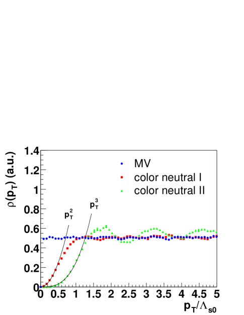
Figure 1: Color Charge Correlator in momentum space. Original MV model is shown by circles, while squares correspond to the result from color neutrality condition I and triangles correspond to color neutrality condition II (see text). The color charge correlator is plotted versus $p_{T}$ in units of $\Lambda_{s0}$.

In Fig. 1, we plot the Fourier transform of the charge correlator, which in the continuum is defined as

$$\tilde{\rho}(p_{T})=\,\int d^{2}x_{T}\exp(i\bm{p}_{T}\cdot\bm{x}_{T})\langle\rho^{a}(x_{T})\rho^{a}(0)\rangle\,,$$ (10)

for the MV model and for the two variants which impose color neutrality on the nucleon level. In the MV model, it is evident from Eq. (2) that $\tilde{\rho}(p_{T})$ is a constant everywhere except at $p_{T}=0$ where it is constrained to be zero from the global charge constraint. In the Color Neutral I (II) variant, we see that $\tilde{\rho}(p_{T})\sim p_{T}^{2}$ ($\sim p_{T}^{3}$) for small momenta $p_{T}<\Lambda_{s0}$ and is constant at larger momenta. The oscillatory behavior seen for Color Neutral I and II is due to the fact that the correlator in coordinate space is not strictly a delta-function. In the coordinate space the charge correlator for the two models, Color Neutral I and II, falls off rapidly, as $\sim 1/x_{T}^{4}$ and $\sim 1/x_{T}^{5}$ respectively, at larger distances.

It is an interesting coincidence that the behavior of $\tilde{\rho}(p_{T})$ in our model is similar to the behavior expected from the renormalization group (RG) evolution of color charges in the McLerran-Venugopalan model. In Ref. ILM , it is shown that the screening of color charges due to the RG evolution gives a behavior $\tilde{\rho}(p_{T})\sim p_{T}^{2}$ for $p_{T}\leq\Lambda_{s0}$ (and $\tilde{\rho}(p_{T})$=constant for $p_{T}>\Lambda_{s0}$). A recent analysis by Mueller gives the same result with a specific prediction for the prefactor Mueller2002 . These results lie between the range spanned by our “Color Neutral I” and “Color Neutral II”. Since the only information on the RG in our formalism for nuclear collisions comes from the initial conditions, our results may be quantitatively similar to RG evolved predictions for nuclear collisions.

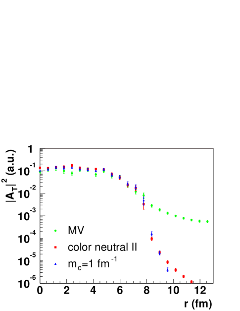
Figure 2: Gluon field as a function of radial distance. Original MV model is shown by circles, while squares correspond to the Color Neutral II prescription (see text). Results from Eq. (13) are shown by triangles. The results are for $\Lambda_{s0}R=18.5$.

We now discuss how the gauge fields are determined from the color charge distributions. The pure gauges at the site $j$ are defined with Hermitian traceless matrices $\Lambda_{j}$ on the lattice as

$$U_{\hat{n},j}=\exp[i\Lambda_{j+\hat{n}}]\exp[-i\Lambda_{j}].$$ (11)

$\Lambda_{j}$ can be obtained by solving the lattice Poisson equation

$$-\Delta_{L}\Lambda_{j}\equiv-\sum_{n=\hat{x},\hat{y}}\left(\Lambda_{j+n}+\Lambda_{j-n}-2\Lambda_{j}\right)=\rho_{j}.$$ (12)

We solve Eq. (12) numerically, using the fast Fourier transform (FFT) method which is faster than the approach employed in Ref. AR99 . Imposing color neutrality on the nucleon level (for both Color Neutral I and Color Neutral II) significantly suppresses the gluon field outside the color charge density as shown in Fig 2.

One can also simulate our color neutrality prescription by introducing a screening mass $m_{c}$ to the Poisson equation Eq. (12)

$$(-\Delta_{L}+m_{c}^{2})\Lambda_{j}=\rho_{j},$$ (13)

as a simple method to suppress the gluon field. The range of the screening mass must be $m_{c}\sim\Lambda_{QCD}$. Although this procedure does not originate in any color-neutrality condition, it is clear that the gluon distribution at high momentum range should not be modified, since $|A_{T}(p_{T})|^{2}\sim 1/(p^{2}_{T}+m_{c}^{2})$. Fig 2 demonstrates that the gluon field distribution with $m_{c}=1.0\text{ fm}^{-1}$ is nearly identical to the color neutral distribution.

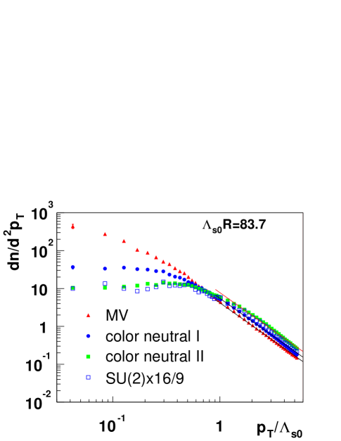
Figure 3: Comparison of the unintegrated gluon distribution before the collision obtained by the simple MV model (triangles), color neutral I (circles) and color neutral II (full squares). The SU(2) result scaled by 16/9 is shown in open squares. The line corresponds to a $1/p_{T}^{2}$ distribution. Results are for $\Lambda_{s0}R=83.7$.

In Fig. 3, we plot numerical results for the SU(3) unintegrated gluon transverse momentum distributions before the collision. The gluon distributions from models which impose strict color neutrality at the nucleon level are significantly suppressed at momenta $p_{T}<\Lambda_{s0}$ compared to that of the original MV model which had only a global color neutrality constraint for the nucleus. In the large momentum region, where we expect the color neutrality constraints to be immaterial, both sorts of models show the same $1/p_{T}^{2}$ dependence. Comparing the SU(2) result for the Color Neutral II model to the SU(3) result, we observe that the ratio of the two results is the ratio of the respective Casimirs. The results shown in the figure are all for one value of the dimensionless coupling $\Lambda_{s0}R$. The qualitative results are the same for other values of this parameter.

II.2 Nuclear collisions

We can now apply our model for parton distributions of finite ultrarelativistic nuclei to discuss classical gluon production in nuclear collisions. This problem was first formulated by Kovner, McLerran and Weigert KMW and perturbative solutions were discussed further by several authors DYEA ; GyulassyMcLerran ; Balitsky . The numerical formulation of the classical problem has been discussed extensively by us in previous papers AR99 ; AR00 ; AR01 ; AYR01 . In these papers, we considered, for simplicity, only the case of cylindrical nuclei with uniform nuclear matter distributions. Periodic boundary conditions were imposed. We will discuss here the formulation of the problem for finite nuclei and open boundary conditions. In the previous sub-section, we obtained the color charge and gluon distributions in coordinate space and momentum-space after applying color neutrality prescriptions at the nucleon level. These distributions then give us the necessary ingredients to discuss the space-time evolution of classical fields after the collision. For completeness (and continuity) we will repeat some of the arguments in the papers cited here.

We fix the gauge condition to be the radiation gauge $A^{\tau}=0$ or equivalently,

$$x^{+}A^{-}+x^{-}A^{+}=0.$$ (14)

We require that the light cone color charges on each light cone are delta function sources: $J^{\pm,a}=\delta(x^{\mp})\rho^{\pm,a}(x_{T})$-the solutions to the Yang-Mills equations are then explicitly boost invariant. We are interested in the physics pertaining to the mid-rapidity region and will consider the space-time rapidity $\eta$ to be zero. Our ansatz for the gauge field as a function of proper time $\tau=\sqrt{2x^{+}x^{-}}$ is

$$A^{i} = \alpha^{i}_{3}(\tau,x_{T})\theta(x^{-})\theta(x^{+})$$ (15a)

$$+ \alpha^{i}_{1}(\tau,x_{T})\theta(x^{-})\theta(-x^{+})$$

$$+ \alpha^{i}_{2}(\tau,x_{T})\theta(-x^{-})\theta(x^{+}),$$

$$A^{\pm} = \pm x^{\pm}\alpha(\tau,x_{T})\theta(x^{-})\theta(x^{+}).$$ (15b)

The boundary conditions are determined by matching the solutions in the space-like and time-like regions. Requiring that the gauge fields must both be regular at $\tau=0$, $D_{\mu i}F^{\mu i}=0$ and $D_{\mu+}F^{\mu+}=J^{+}$ for $x^{-},x^{+}\to 0$ gives the boundary conditions at $\tau=0$:

$$\alpha^{i}_{3}(0,x_{T}) = \alpha^{i}_{1}(0,x_{T})+\alpha^{i}_{2}(0,x_{T}),$$ (16a)

$$\alpha(0,x_{T}) = {i\over 2}[\alpha^{i}_{1}(0,x_{T}),\alpha^{i}_{2}(0,x_{T})].$$ (16b)

Note that these conditions, first formulated for infinitely large nuclei, are the same for finite nuclei. There is no ambiguity in determining the reaction zone since, for example, when $\alpha^{i}_{1}=0$, we have $\alpha=0$, $\alpha^{i}_{3}=\alpha^{i}_{2}$, a pure gauge-hence there is no classical gluon production outside the reaction zone.

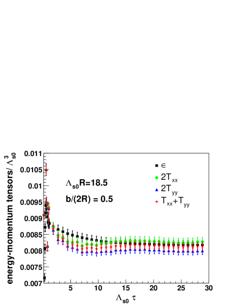
Figure 4: The two components of the transverse pressure ($T_{xx}$ and $T_{yy}$) and the energy density $\epsilon$ plotted as a function of $\tau$ in dimensionless units. The results are for a impact parameter $b=R$ and dimensionless coupling $\Lambda_{s0}R=18.5$. Also shown is the sum of the two transverse pressures.

We shall now explain how one generates the reaction zone in the model. The initial conditions (at $\tau=0$) can be generated in two possible ways.

• For a given impact parameter $b$, one determines the number of participant nucleons using the Glauber model as for example in Ref. KN . The corresponding color charge density (and the gluon distribution) for each nucleus in the reaction zone can then be determined using the sampling procedure described previously. The matching condition in Eq. (16) is then used to determine the initial conditions for the evolution.

• The color charge distribution is determined separately for each nucleus by projecting the color charge distributions of all the color neutral nucleons in the transverse plane. The gluon distribution for each nucleus is then determined accordingly, and the reaction zone is automatically given by the matching condition in Eq. (16) for a specified impact parameter $b$.

The reaction zone can be determined naturally from the procedure (b) as long as we have the correct color charge distribution for a finite nucleus, since the region of $A_{1}=0$, $A_{2}$ remains pure gauge. Nevertheless, we would like to use (a) for purely technical reasons, namely, since it is more efficient for numerical computations. We have checked that the two procedures give nearly identical results.

Explicit expressions for the discretized lattice Hamiltonian, for other components of the stress-energy tensor, and the classical equations of motion can be found in the appendix. In Fig. 4, we plot the temporal behavior of the two transverse pressures and the energy density. Interestingly, at late times we notice that $\epsilon=T_{xx}+T_{yy}$ as one would anticipate for a free streaming gas of gluons in the transverse plane. We will return to this result later. The difference between the two transverse pressures, $\epsilon_{p}=T_{xx}-T_{yy}$ is a measure of the azimuthal anisotropy generated by classical fields AYR02 .

III Impact parameter dependence of multiplicity distributions

In previous papers AR00 ; AR01 ; AYR01 , we compared our results for cylindrical nuclei with periodic boundary conditions and uniform nuclear matter distributions to the RHIC data. In this section, we will apply the more realistic framework developed in the previous section to compute the gluon multiplicity distributions as a function of centrality. If one assumes parton-hadron duality, these distributions can be compared, for instance, to the centrality dependence of the charged hadron spectra in heavy ion collisions at RHIC KN .

At late times $\tau\gg 1/\Lambda_{s0}$, the dynamics of the classical Yang-Mills fields produced in the collision can be linearized and approximated by that of a system of weakly coupled harmonic oscillators. In previous papers AR01 ; AYR01 , we discussed two methods to compute the gluon number. Both of these are applicable when the harmonic oscillator approximation is a good one. One method is a gauge invariant relaxation method which can only be used to measure the particle number and not its distribution with momenta. The other method is to fix the Coulomb gauge and compute the field amplitudes squared in momentum space. We showed that both methods give results for the gluon number which agree very well with each other.

We will therefore restrict ourselves in this paper to using one method alone-that of fixing the transverse Coulomb gauge $\bm{\nabla}_{\perp}\cdot\bm{A}=0$ AR01 and computing the field amplitudes. We have

$$N(k)=\omega(k)\langle|\phi(k)|^{2}\rangle=\sqrt{\langle|\phi(k)^{2}|\rangle\langle|\pi(k)|^{2}\rangle},$$ (17)

where $\phi(k)$ and $\pi(k)$ correspond to the potential term and the kinetic term in the Hamiltonian respectively. The average $\langle\rangle$ represents an average over the initial conditions.

Table 1: $\Lambda_{s0}=1.41$ GeV. Results are for a $256\times 256$ lattice-the nuclear radius is 64 lattice units. All dimensionful scales are in GeV units unless otherwise stated.

$b(fm)$	$N_{part}$	$g^{2}N_{g}$	$g^{2}E_{g}$	$\Lambda(b)$	$Q_{s}(b)$	$f_{N}(b)$
0.000	377.89	1628.68	2725.40	1.1777	1.0836	0.3695
3.150	321.35	1309.83	2170.08	1.1545	1.0563	0.3484
4.725	263.33	1035.84	1663.88	1.1234	1.0197	0.3359
6.300	199.11	760.95	1182.02	1.0741	0.9623	0.3249
7.875	136.47	515.61	751.902	0.9993	0.8758	0.3152
9.450	81.21	295.76	384.004	0.8876	0.7487	0.3004

Table 2: $\Lambda_{s0}=2.32$ GeV. Results are for a $512\times 512$ lattice-the nuclear radius is 128 in lattice units. All dimensionful scales are in GeV units unless otherwise stated.

$b(fm)$	$N_{part}$	$g^{2}N_{g}$	$g^{2}E_{g}$	$\Lambda(b)$	$Q_{s}(b)$	$f_{N}(b)$
0.000	377.89	3768.00	9198.736	1.9517	2.0355	0.2867
3.150	321.35	3061.59	7492.084	1.9132	1.9866	0.2757
6.300	199.11	1808.89	4183.888	1.7800	1.8185	0.2610
7.875	136.47	1215.17	2636.300	1.6560	1.6636	0.2522
8.367	118.17	1042.54	2243.692	1.6060	1.6017	0.2514
9.450	81.21	699.95	1411.900	1.4708	1.4356	0.2411

In Refs. AR01 ; AYR01 , non-perturbative relations were derived for the energy and number of produced gluons (at central rapidities) as a function of $\Lambda_{s}^{2}$. For realistic nuclei, these non-perturbative relations are less simple. One can parametrize our results for the gluon number with the more general relation

$${dN_{g}\over d\eta}=f_{N}(b)\int d^{2}x_{T}{\Lambda_{s}^{2}(b,x_{T})\over g^{2}},$$ (18)

where $\Lambda_{s}(b,x_{T})$ is the local saturation scale defined to be $\Lambda_{s}^{2}(b,x_{T})=C\cdot{\tilde{\rho}}(b,x_{T})/2$, where ${\tilde{\rho}}$ is the participant density at a particular position in the transverse plane, and $C$ is the color charge squared per nucleon. When $\Lambda_{s}(b,x_{T})$=constant, as for cylindrical uniform nuclei, one recovers the form of the expressions in Refs. AR01 ; AYR01 . The color charge squared in the center of the nucleus is $\Lambda_{s0}^{2}=C\cdot{\tilde{\rho}}(0,0)/2$, so $\Lambda_{s}^{2}(b,x_{T})=\Lambda_{s0}^{2}{\tilde{\rho}}(b,x_{T})/{\tilde{\rho}}(0,0)$. One can then re-write the previous equation as

$${dN_{g}\over d\eta}={f_{N}(b)\over g^{2}}{\Lambda_{s0}^{2}\over\rho_{0}}N_{part}(b),$$ (19)

where $\rho_{0}={\tilde{\rho}}(0,0)=4.321\text{ fm}^{-2}$ and $N_{part}=\int d^{2}x_{T}{\tilde{\rho}}(b,x_{T})$.

In Tables 1 and 2, we show the calculated SU(3) results for two values of the saturation scale in the center of the nucleus: $\Lambda_{s0}=1.41$ and $\Lambda_{s0}=2.32$ GeV respectively. In the tables, $b$ is an impact parameter (in units of fm) and $N_{part}$ is a number of participants at that impact parameter. The latter is calculated using a Woods-Saxon nuclear density profile. We list in the tables our results, as a function of impact parameter, for $g^{2}N_{g}$; the number of produced gluons and $g^{2}E_{g}$; the transverse energy of produced gluons in GeV multiplied by the value of the strong coupling constant squared $g^{2}$, evaluated (to one loop order) at the average value of the saturation scale (denoted in the tables as $Q_{s}(b)$) for that impact parameter.

In Table 1, we see that the gluon multiplicity, for the most central collisions, is about half the final pion multiplicity at RHIC while the transverse energy of gluons is close to the experimentally observed transverse energy of about $600$ GeV. In Table 2, the gluon multiplicity is close to the final pion multiplicity at RHIC while now the transverse energy is nearly four times larger than the experimentally observed transverse energy. Neither the initial transverse energy nor the initial gluon multiplicity are conserved quantities, so the results for different values of the saturation scale lend themselves to very different dynamical scenarios. For instance, the authors of Ref. BMSS have suggested that inelastic $gg\rightarrow ggg$ processes may be important in the early stages of nuclear collisions thereby increasing the gluon multiplicity prior to thermalization/hadronization. Alternatively, if the gluon number close to the experimental number (as in Table 2), strong hydrodynamic expansion at early times might be essential to lower the initial transverse energy to the experimentally desired value. Additional observables (such as $v_{2}$) may be important in distinguishing between the different scenarios.

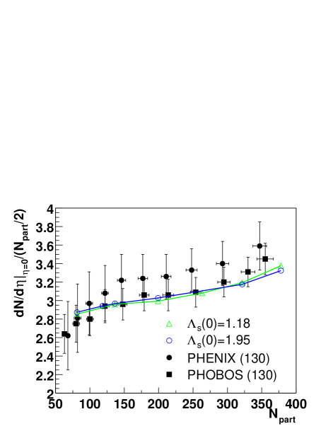
Figure 5: Comparison of the centrality dependence of the gluon distribution from SU(3) lattice results to data from experiments phenix_mult ; phobos130 . The strong coupling constant is fixed to the value $g^{2}=4$. The lattice results for $\Lambda_{s}(0)=1.18$ GeV and $\Lambda_{s}(0)=1.95$ GeV are multiplied by a factor 2.4 and 1.1, respectively.

In Fig 5, we plot the centrality dependence of gluons calculated using Eq. (17) together with the experimental data from PHOBOS phobos130 and PHENIX phenix_mult . We assume here that the charged particle multiplicity is two thirds of the gluon number. The classical computation is performed for fixed $\alpha_{s}$; the centrality dependence, as seen from Eq. (19), comes from the dependence of $f_{N}$ on the impact parameter. In Ref. AR01 , it was shown that $f_{N}\equiv f_{N}(\Lambda_{s}R)$ increases slowly with $\Lambda_{s}R$-hence one expects it to vary with impact parameter. We see that the results agree reasonably well with the data.

The centrality dependence of the transverse energy is studied in Fig. 6. As in the case of the multiplicity, even though the absolute normalization is strongly dependent on one’s choice of $\Lambda_{s}$, the centrality dependence is very similar for the two $\Lambda_{s}$’s and shows reasonable agreement with the data.

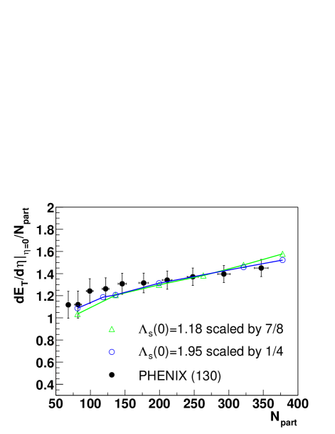
Figure 6: Comparison of the centrality dependence of the gluon transverse energy distribution from SU(3) lattice results to data from experiments phenix_et . The strong coupling constant is fixed to the value $g^{2}=4$. The lattice results for $\Lambda_{s}(0)=1.95$ GeV are scaled by ${1\over 4}$ while those for $\Lambda_{s}(0)=1.18$ are scaled by ${7\over 8}$.

Let us now compare our results with those derived in Ref. KNL and discussed further in Ref. BMSS2 . In these works, one obtains in terms of ${\bar{Q_{s}}}$, the average saturation scale, the result

$${dN_{g}\over d\eta} = c_{N}\frac{N_{c}^{2}-1}{4\pi^{2}N_{c}}\int d^{2}x_{T}{Q_{s}^{2}(b,x_{T})\over\alpha_{s}}$$ (20)

$$\approx c_{N}xG(x,{\bar{Q}_{s}}^{2}(b))\frac{N_{part}}{2}\,.$$

In the leading logarithmic approximation, if $c_{N}$ is constant, one obtains a logarithmic dependence on the centrality entirely from $xG(x,{\bar{Q}_{s}^{2}(b)})$. One could thus attribute the logarithmic behavior at the classical level to fixed $\alpha_{s}$ and leading logarithmic behavior of the gluon distribution function or equivalently, at higher order, to the one loop running of $\alpha_{s}$. In the physically interesting regime, it is difficult to distinguish between the two. A reasonable agreement with the data is also seen in this formulation of the problem.

The relation between the two formulations is as follows. As discussed previously, what we simulate numerically is the color charge squared per unit area, $\Lambda_{s}^{2}$ AR01 . The saturation scale, on the other hand, is a scale determining the behaviour of the gluon number distribution KovMuell . The two scales can be related by computing, for instance, the gluon number distribution in a nucleus in the McLerran-Venugopalan approach (where $\Lambda_{s}$ naturally appears) and in Mueller’s dipole approach. On comparing the two one obtains, to leading logarithmic accuracy, the following relation between $\Lambda_{s}$ and $Q_{s}$:

$$Q^{2}_{s}={N_{c}\Lambda_{s}^{2}\over 4\pi}\log\left({\Lambda_{s}^{2}\over\Lambda^{2}_{QCD}}\right),$$ (21)

with $\Lambda_{QCD}=0.2$ GeV. The relation between $c_{N}$ and $f_{N}$ is $c_{N}=4\pi^{2}f_{N}/(N_{c}^{2}-1)/\ln(Q_{s}^{2}/\Lambda_{QCD}^{2})$. Therefore, if $c_{N}$ is to be a constant, $f_{N}$ increases logarithmically with $Q_{s}$. A weak rise in $f_{N}$ is seen in our simulations. If the infrared scale, as argued in Ref. KIIM , is a number of order $O(1/Q_{s})$, we would have $\Lambda_{s}\approx Q_{s}$. Note that in practice $Q_{s}^{2}(b)$ and $\Lambda_{s}^{2}(b)$ (related by Eq. (21) are nearly equal to each other for all impact parameters.

In Ref. BMSS , it was argued that subsequent inelastic scattering of gluons after the classical approximation is applicable but before thermalization would increase the multiplicity by a factor $1/\alpha_{s}^{2/5}$. This effect was taken into account in Ref. BMSS2 and it was shown that good fits to the data could be obtained for this functional form as well. The effects of parton multiplication a la Ref. BMSS2 are beyond the scope of this work and we will not discuss it further here.

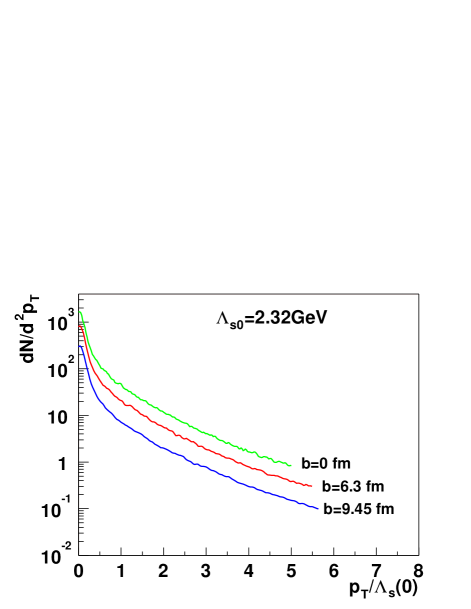
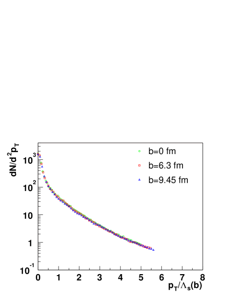
Figure 7: Top: Gluon transverse momentum distributions as a function of $p_{T}/\Lambda_{s}(b)$ for $b=0.0$, 6.4, and 9.45 fm. Bottom: Same as top figure but with re-scaled normalizations.

We now turn to the computation of the initial gluon transverse momentum distributions. In the top half of Fig. 7, we show the initial gluon transverse momentum distributions for different impact parameters in dimensionless units of $p_{T}/\Lambda_{s}(b)$. In the bottom half of the figure we plot the same quantity by re-scaling the overall normalization of the distributions. Strikingly, as a consequence of geometrical scaling, the distributions now coincide-the initial gluon distributions are a universal function of $p_{T}/\Lambda_{s}(b)$. In Ref. Juergen , it was argued that the RHIC data display such a geometrical scaling. More detailed comparisons with the recent RHIC data at $\sqrt{s_{NN}}=200$ GeV will help further clarify the observation of geometrical scaling. Note however that the typical $\langle p_{T}\rangle$ of the initial gluon distribution is of order $\Lambda_{s}$, while the observed $\langle p_{T}\rangle$ of charged hadrons is smaller, of the order $3T_{c}$. For the $\Lambda_{s}$ in Table 1, this difference is a factor of two; for those in Table 2, it is significantly larger.

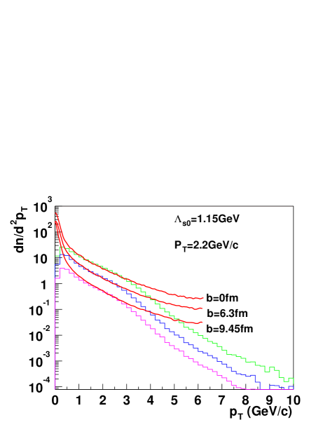
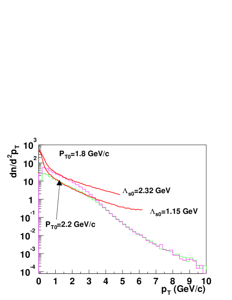
Figure 8: Top: Gluon transverse momentum distributions at $\eta=0$ for impact parameters $b=0$, 6.3, 9.45 fm in the case of $\Lambda_{s0}=1.15$ GeV. Mini-jet partons from PYTHIA, multiplied by number of collisions, with cut-off momentum $p_{T}=2.2$ GeV/c, are also plotted in histograms. Bottom: The same for impact parameters $b=0$ fm for $\Lambda_{s0}=1.15$ GeV and $\Lambda_{s0}=2.23$ GeV. Different cut-off momenta of $p_{T}=2.2$ and $p_{T}=1.8$ GeV/c for the PYTHIA mini-jets are also plotted by histograms.

It is instructive to compare the transverse momentum distributions computed in the classical approach with the pQCD computations of the gluon distribution. The latter is obtained as follows. In the parton model, when the parton density is small, the cross section for hard parton scattering can be calculated as

$${d\sigma_{jet}\over dp^{2}_{T}dy_{1}dy_{2}}=K\sum_{a,b}x_{1}x_{2}f_{a}(x_{1},Q^{2})f_{b}(x_{2},Q^{2}){d\sigma_{ab}\over d\hat{t}}\,,$$ (22)

where $y_{1}$ and $y_{2}$ are the rapidities of the scattered partons and $x_{1}$ and $x_{2}$ are the fractions of momentum of the initial partons. The structure functions, $f_{a}(x,Q^{2})$ are taken to be the CTEQ5 leading order parametrizations cteq5 . The parton distributions are evaluated at the scale $Q^{2}=p_{T}^{2}$. Here $d\sigma_{ab}/d\hat{t}$ is the leading order QCD partonic cross section. In addition, one includes initial and final state radiation processes in order to take into account the enhancement of higher-order contributions associated with multiple small-angle parton emission. This is for instance what is done in the event generator PYTHIA and we use for our purposes PYTHIA version 6.2 pythia for the incident c.m. energy of $\sqrt{s}=130$ GeV. The $K$ factor of $K=2$ is chosen to fit the UA1 data of $p\bar{p}$ at $\sqrt{s}=200$ GeV ua1 . The nuclear gluon distributions are obtained by multiplying the PYTHIA result by the number of hard binary collisions. Nuclear shadowing effects are neglected.

In the top half of Fig. 8, we study the impact parameter dependence of the classical gluon transverse momentum distributions (with $\Lambda_{s0}=1.14$ GeV) together with the parton distributions from PYTHIA calculations with an infrared cut-off parameter of $p_{T}=2.2$ GeV/c. We find that there is a overlap region between 1-3 GeV/c between the two computations. For higher transverse momenta, the classical computation overshoots the PYTHIA result. One reason this is the case is that the realistic parton distributions have not been included in the classical distribution-this makes a difference at large transverse momenta GyulassyMcLerran ; DJLT . Naively, one would expect the pQCD result to diverge rapidly at small $p_{T}$. The reason it doesnt is that initial and final state radiation processes change the parton distributions from Eq. (22) below 3-4 GeV/c. In the lower half of Fig. 8, we plot the gluon distributions with the parameters $\Lambda_{s0}=2.32$ and 1.14 GeV along with the PYTHIA gluon distributions for different values of the infrared cut-off. The latter is not an infrared safe quantity so it is not too surprising that the shape and magnitude of the distribution does depend on the cut-off. So if one were to match the classical and pQCD distributions, one has to adjust the $p_{T}$ cut-off for different values of $\Lambda_{s0}$. The differences in the gluon number between the classical and classical+PYTHIA LO pQCD result are not very significant for the particle number but may be so for the transverse energy since the latter is more ultraviolet sensitive. Therefore the large transverse energy per particle obtained in the classical approach may be significantly overestimated. A more realistic calculation of the distribution of hard modes will find less of an excess (relative to experiment) in the transverse energy.

We discussed in this section our results from numerical simulations of very high energy nuclear collisions of nuclei at various impact parameters. While the absolute numbers from our results depend very sensitively on the scale $\Lambda_{s}$, the dependence of the gluon number and transverse energy on centrality and the phenomenon of geometrical scaling of the momentum distributions are independent of $\Lambda_{s}$ and appear universal. In addition, they appear to agree reasonably well with trends in the RHIC data. Similar observations were made in Refs. KN ; KNL and in Ref. Juergen for global features of the data.

IV proton-nucleus collisions

Collisions of protons/deuterium with large nuclei at RHIC energies are essential to distinguish dynamical effects due to correlations in the nuclear wavefunction from dynamical effects resulting from the collective expansion of hot and dense matter in nucleus-nucleus collisions. The first computation, in the classical framework, of gluon production was performed by Kovchegov and Mueller KovMuell . Here we will follow the subsequent work of Dumitru and McLerran Dumitru which is closer in its formulation to the discussion here. In Ref. Dumitru , the authors introduce two saturation scales which we will denote as $\Lambda_{s1}$ (for the proton) and $\Lambda_{s2}$ for the nucleus. One expects that since the parton density in a nucleus is larger than in a proton, $\Lambda_{s1}^{2}\ll\Lambda_{s2}^{2}$. In the kinematic region $p_{T}>\Lambda_{s1}$, analytical computations of gluon production are feasible. For $\Lambda_{s1}<\Lambda_{s2}<p_{T}$, the situation is analogous to nucleus-nucleus collisions and the distributions are proportional to $\Lambda_{s1}^{2}\Lambda_{s2}^{2}/p_{T}^{4}$. For $\Lambda_{s1}<p_{T}<\Lambda_{s2}$, the distribution changes qualitatively and is proportional to $\Lambda_{s1}^{2}/p_{T}^{2}$. In this kinematic region, one obtains Ad:note $dN/d^{2}b\,d^{2}k_{t}\propto\Lambda_{s1}^{2}\ln(k_{t}^{2}/\Lambda_{s1}^{2})/k_{t}^{2}$.

In our framework, $pA$ collisions can be simulated straightforwardly since the only change from nucleus-nucleus collisions is to consider asymmetric values of $\Lambda_{s}$. The results of our simulations are shown in Fig. 9. We choose a fixed value for $\Lambda_{s02}$ in the center of the nucleus and plot the momentum distributions for different $\Lambda_{s01}$’s. At large $p_{T}$, as anticipated, the distribution goes as $1/p_{T}^{4}$. At smaller $p_{T}$ of $p_{T}\sim 2\Lambda_{s02}$ one sees a qualitative change in the distributions which is more consistent with a $1/p_{T}^{2}$ behavior of the distributions. Thus it appears that our distributions reproduce the shapes predicted by Dumitru and McLerran in the appropriate kinematical regions.

A comparison of absolute normalizations is more tricky. If one computes analytically Ad:note the ratio of the multiplicities at the scale $k_{t}\sim\Lambda_{s02}$ for the two values of $\Lambda_{s01}$ shown in Fig. 9, the ratio is $\sim 23$, which is the scaling factor used to scale the distribution with the lower $\Lambda_{s01}$ to that with the larger value. However, we should caution that the absolute normalization of these results is uncertain because the behavior in the kinematic region $p_{T}<\Lambda_{s01}$ cannot be computed analytically comment1 and can only be computed numerically as discussed here.

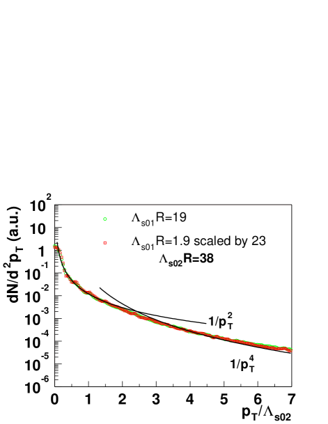
Figure 9: Transverse momentum distribution of produced gluons in a pA collision. Here $\Lambda_{s01}^{2}$ refers to the color charge squared per unit area in the center of the proton while $\Lambda_{s02}^{2}$ is the color charge squared per unit area in the center of a nucleus.

More detailed studies of pA collisions are underway and will be reported separately AYR03 .

V Summary

In this paper, we extended previous results for collisions of uniform, cylindrical nuclei with periodic boundary conditions to finite nuclei with realistic nuclear matter distributions and open boundary conditions. To achieve this, we imposed color neutrality constraints on nucleon color charge distributions. With these improvements, we were able to study nuclear collisions at different impact parameter and proton-nucleus collisions. We obtained results for the initial gluon number and transverse energy and compared these to the data. While the absolute normalizations of these quantities depend sensitively on the saturation scale $\Lambda_{s}$, their centrality dependence appears universal and shows reasonable agreement with the experimental data. Similarly, the transverse momentum distributions display geometrical scaling. (The latter has been argued to be a feature of the RHIC data Juergen .) Our results however also suggest that dynamical effects at later times (possibly beyond the validity of the classical approach) might also be important in describing the RHIC data in detail. This is suggested for instance by the necessity of reproducing both the transverse energy and the multiplicity but more emphatically by the failure of the classical approach to explain the elliptic flow data AYR02 . It has been argued that the elliptic flow data may be explained by non-flow correlations KT but more detailed theoretical and experimental analyses are required to clarify the issue.

We also briefly discussed proton-nucleus collisions in the classical framework. We showed that our numerical simulations agree qualitatively with previous analytical work KovMuell ; Dumitru . This agreement suggests that results of our numerical simulations for nucleus-nucleus collisions (where analytical computations are more difficult) are robust.

The classical distributions discussed here can be used as the initial conditions for the subsequent time evolution of produced gluons as might be described, for instance, in Boltzmann type transport calculations Mueller1 ; MBVDG ; BMSS ; Nara:2001zu at late times where field strengths are weak. With these initial conditions, it will be interesting to study the consequences of parton evolution on flow or parton energy loss.

The classical treatment of nuclear collisions can also be improved significantly. One such improvement is to give up the assumption of strict boost invariance and to study the effects of doing so on our distributions. Another is to go beyond the simple assumption of Gaussian-distributed color charges and to incorporate the effects of renormalization group evolution of the color charges at high energies. All of these studies, tempered by the large amount of available experimental data, will hopefully provide insight into the very earliest moments of a high energy nuclear collision and of the subsequent dynamics of the produced quark gluon matter.

*

Appendix A Space-time evolution of the Stress-Energy tensor in a nuclear collision

For completeness, we provide in this appendix explicit expressions for the lattice Hamiltonian, the lattice equations of motion and discretized expressions for other components of the Stress-Energy tensor for the problem of interest.

A.1 Hamiltonian approach in the transverse plane

In this sub-section, we write down the classical Hamiltonian’s equations of motion in the $\tau,\eta,\vec{r}$ coordinates where $\tau=\sqrt{2x^{+}x^{-}}$ is the proper time, $\eta={1\over 2}\log(x^{+}/x^{-})$ is the space-time rapidity and $\vec{r}=(x,y)$ are two transverse Euclidean coordinates. Inverse transformations are $t=\tau\cosh\eta$ and $z=\tau\sinh\eta$ respectively. The QCD action for gauge field in the $\tau,\eta,\vec{r}$ coordinates reads

$$S_{QCD}=\int\tau d\eta d\tau d^{2}r\left[-{1\over 8}\text{Tr}(g^{\mu\alpha}g^{\nu\beta}F_{\alpha\beta}F_{\mu\nu})\right],$$ (23)

where $F_{\mu\nu}=\partial_{\mu}A_{\nu}-\partial_{\nu}A_{\mu}-ig[A_{\mu},A_{\nu}]$ and the metric is diagonal with $g^{\tau\tau}=-g^{xx}=-g^{yy}=1$ and $g^{\eta\eta}=-1/\tau^{2}$. $A_{\mu}\equiv A_{\mu}^{a}t^{a}$, and $t^{a}$ represent a gauge group matrices with the normalization of $\text{Tr}(t^{a}t^{b})=2\delta_{ij}$. The Lagrangian density in $A^{\tau}=0$ gauge is

$${\cal L}=\text{Tr}\left({\tau\over 4}(\partial_{\tau}A_{i})^{2}+{1\over 4\tau}(\partial_{\tau}A_{\eta})^{2}-{\tau\over 8}F_{ij}^{2}-{1\over 4\tau}F_{\eta i}^{2}\right)\,,$$ (24)

where $i,j$ runs over transverse coordinate $x$ and $y$.

Now let us assume $\eta$ independence of the fields. As discussed previously, the Yang-Mills equations have this property if the sources are strictly $\delta$-function sources on the light cone. We have

$$A_{i}(\tau,\eta,{\vec{r}})=A_{i}(\tau,{\vec{r}}),\qquad A_{\eta}(\tau,\eta,{\vec{r}})=\Phi(\tau,{\vec{r}})\,,$$ (25)

resulting in $F_{\eta i}=-D_{i}\Phi$, where $D_{i}=\partial_{i}-ig[A_{i},\cdots]$ is the covariant derivative in the adjoint representation. Defining the conjugate momenta

$$E_{i}=\tau\partial_{\tau}A_{i},\quad p_{\eta}={1\over\tau}\partial_{\tau}A_{\eta}\,,$$ (26)

one finds that the boost invariant Yang-Mills Hamiltonian is the QCD Hamiltonian in 2+1 dimensions coupled to an adjoint scalar AR99 :

$$H=\int d^{2}r\text{Tr}\left\{{1\over 4\tau}E_{i}^{2}+{\tau\over 4}p_{\eta}^{2}+{\tau\over 8}F_{ij}^{2}+{1\over 4\tau}(D_{i}\Phi)^{2}\right\}\,.$$ (27)

The equations of motion corresponding to this Hamiltonian are

$$\dot{A_{i}} = {E_{i}\over\tau},\quad\dot{\Phi}=\tau p_{\eta},\quad(i=x,y),$$

$$\dot{E_{x}} = -\tau D_{y}F_{xy}+{ig\over\tau}[\Phi,D_{x}\Phi],$$

$$\dot{E_{y}} = \tau D_{x}F_{xy}+{ig\over\tau}[\Phi,D_{y}\Phi],$$

$$\dot{p}_{\eta} = {1\over\tau}(D_{x}^{2}\Phi+D_{y}^{2}\Phi),$$

and the Gauss law constraint is

$$\bm{D}\cdot\bm{E}+ig[p_{\eta},\Phi]=0\,.$$ (29)

A.2 Discretized Hamiltonion formalism in 2+1 dimensions

In order to realize numerically the solutions to the equations of motion in the previous section, while maintaining the gauge symmetry, we introduce the link variables at the site $i$

$$U_{j,i}=\exp\left[igaA_{j}(i)\right],\quad(j=x,y),$$ (30)

where, $a$ is a lattice spacing. Defining the plaquette

$$U_{\Box}\equiv U_{l,j}U_{m,j+l}U^{\dagger}_{l,j+m}U^{\dagger}_{m,j}\,,$$ (31)

the magnetic energy in the transverse plane is expressed for $a\to 0$ as

$${\tau\over 2a^{2}g^{2}}\sum_{\Box}(N_{c}-\rm{ReTr}U_{\Box}),$$ (32)

where the relation $U_{\Box}=\exp[ia^{2}gF_{\mu\nu}]$ was used. The Hamiltonian on the lattice is

$$H_{L} = {1\over 4\tau}\sum_{\ell\equiv(j,\hat{n})}{\rm Tr}E_{\ell}^{2}$$ (33)

$$+ {\tau\over 2}\sum_{\Box}(N_{c}-{\rm ReTr}U_{\Box})$$

$$+ {1\over 4\tau}\sum_{j,\hat{n}}{\rm Tr}(\Phi_{j}-U_{\hat{n},j}\Phi_{j+\hat{n}}U^{\dagger}_{\hat{n},j})^{2}$$

$$+ {\tau\over 4}\sum_{j}{\rm Tr}p_{j}^{2},$$

where the following dimensionless variables are used  Biro:1993qc ; Heinz:1996wx :

$$H \to {H\over g^{2}a},\quad E\to{E\over ga^{2}},\quad p\to{p\over ga},\quad$$ (34)

$$\Phi \to {\Phi\over ga},\quad\tau\to a\tau.\quad$$

Hamilton’s equations of motion on the lattice are then

$$\dot{U}_{r,i} = -{i\over\tau}U_{r,i}E_{r,i},\quad\dot{\Phi}_{i}=\tau p_{i},\quad(r=x,y),$$

$$\dot{E}^{a}_{x,i} = \tau{-i\over 2}{\rm Tr}t^{a}\Big{\{}U_{y,i+\hat{x}}U^{\dagger}_{x,i+\hat{y}}U^{\dagger}_{y,i}U_{x,i}$$

$$- U_{x,i}^{\dagger}U^{\dagger}_{y,i-\hat{y}}U_{x,i-\hat{y}}U_{y,i+\hat{x}-\hat{y}}\Big{\}}$$

$$+ {ig\over\tau}[\Phi_{i+\hat{x}},U^{\dagger}_{x,i}\Phi_{i}U_{x,i}],$$

$$\dot{E}^{a}_{y,i} = \tau{-i\over 2}{\rm Tr}t^{a}\Big{\{}-U_{y,i+\hat{x}}U^{\dagger}_{x,i+\hat{y}}U^{\dagger}_{y,i}U_{x,i}$$

$$+ U_{x,i+\hat{y}-\hat{x}}^{\dagger}U^{\dagger}_{y,i-\hat{x}}U_{x,i-\hat{x}}U_{y,i}\Big{\}}$$

$$+ {ig\over\tau}[\Phi_{i+\hat{y}},U_{y,i}^{\dagger}\Phi_{i}U_{y,i}],$$

$$\dot{p}_{i} = {1\over\tau}\Big{[}\sum_{\hat{n}=x,y}\big{(}U_{\hat{n},i}\Phi_{\hat{n}+i}U_{\hat{n},i}^{\dagger}+U_{\hat{n},i-\hat{n}}^{\dagger}\Phi_{i-\hat{n}}U_{\hat{n},i-\hat{n}}\big{)}$$ (35)

$$- 4\Phi_{i}\Big{]}.$$

Once one has explicit expressions for the fields and their canonically conjugate momenta, other components of the Stress–Energy tensor can be computed as well. In light-cone coordinates $(\tau,\eta,\vec{r})$, the symmetric energy-momentum tensor can be defined as

$$T^{\mu\nu}=-{\tau\over 2}\text{Tr}(F^{\mu\alpha}F^{\nu}_{\ \alpha})-g^{\mu\nu}{\cal L}\,.$$ (36)

The diagonal spatial components $T^{xx}$ and $T^{yy}$ (the two components of the transverse pressure) are explicitly

$$T^{xx} = {1\over 4}\text{Tr}\Big{(}{1\over\tau}(-E_{x}^{2}+E_{y}^{2}+(D_{x}\Phi)^{2}-(D_{y}\Phi)^{2})$$ (37)

$$+ \tau p_{\eta}^{2}+{\tau\over 2}F_{ij}F_{ij}\Big{)},$$

$$T^{yy} = {1\over 4}\text{Tr}\Big{(}{1\over\tau}(+E_{x}^{2}-E_{y}^{2}-(D_{x}\Phi)^{2}+(D_{y}\Phi)^{2})$$ (38)

$$+ \tau p_{\eta}^{2}+{\tau\over 2}F_{ij}F_{ij}\Big{)}.$$

The $T^{\tau x}$ and $T^{\tau y}$ parts can be calculated as

$$T^{\tau x}=-{1\over 2}\text{Tr}(E_{y}F_{xy}+p_{\eta}(D_{x}\Phi)),$$ (39)

$T^{\tau y}$ is obtained by replacing $x\leftrightarrow y$ in this expression.

The lattice equivalents of these continuum expressions are as follows. The transverse pressure in the $y$ direction is

$$T^{yy}_{i} = {1\over 8\tau}\sum_{j=i,i-\hat{x},i-\hat{y}}\text{Tr}(E_{x,j}^{2}-E_{y,j}^{2})$$ (40)

$$+ {\tau\over 8}\sum_{4\Box}(N_{c}-\text{ReTr}U_{\Box})$$

$$- {1\over 8\tau}\sum_{j=i,i-\hat{x}}\text{Tr}(\Phi_{j}-U_{\hat{x},j}\Phi_{j+\hat{x}}U^{\dagger}_{\hat{x},j})^{2}$$

$$+ {1\over 8\tau}\sum_{j=i,i-\hat{y}}\text{Tr}(\Phi_{j}-U_{\hat{y},j}\Phi_{j+\hat{y}}U^{\dagger}_{\hat{y},j})^{2}$$

$$+ {\tau\over 4}\text{Tr}p_{i}^{2}\,.$$

where $4\Box$ means a sum over the four plaquettes which contain the link $i$ with the same orientations. $T^{xx}$ can be obtained by replacing $x\leftrightarrow y$ in Eq. (40).

One of the ways to get the lattice definition of Poynting vector may be a use of the conservation law $\partial_{\mu}T^{\mu\nu}=0$:

$$\partial_{\tau}T^{\tau\tau}=\partial_{x}T^{\tau x}+\partial_{y}T^{\tau y},$$ (41)

with the $T^{\tau\tau}$ which has to be defined in a local gauge invariant form at a site $i$ as

$$T^{\tau\tau}_{i} = {1\over 8\tau}\sum^{{}^{\prime}}_{\ell=(j,\hat{n})}{\rm Tr}E_{\ell}^{2}+{\tau\over 2}(N_{c}-{\rm ReTr}U_{\Box})$$ (42)

$$+{1\over 4\tau}\sum^{{}^{\prime}}_{j,\hat{n}}{\rm Tr}(\Phi_{j}-U_{\hat{n},j}\Phi_{j+\hat{n}}U^{\dagger}_{\hat{n},j})^{2}$$

$$+{\tau\over 16}\sum^{{}^{\prime}}_{j}{\rm Tr}p_{j}^{2},$$

where $\sum^{{}^{\prime}}_{i}\equiv i+(i+\hat{x})+(i+\hat{y})$. After quite some algebra, we obtain

$$T^{\tau x}_{i} = -{1\over 4}E_{i,x}\Big{[}U_{x,i+y}U_{y,i+x}^{\dagger}U_{x,i}^{\dagger}U_{y,i}$$ (43)

$$+ (U_{y,i}^{\dagger}U_{x,i-x}^{\dagger}U_{y,i-x}U_{x,i-x+y}\Big{]}$$

$$+ {1\over 8}\Big{[}p_{i}(U_{x,i-x}^{\dagger}\Phi_{i-x}-U_{x,i}\Phi_{i})$$

$$+ p_{i+y}(U_{x,i+y-x}^{\dagger}\Phi_{i+y-x}$$

$$\qquad-U_{x,i+y}\Phi_{i+y+x})\Big{]}.$$

References

- (1) L.V. Gribov, E. M. Levin and M. G. Ryskin, Phys. Repts. 100 (1983) 1; A. H. Mueller and J.-W. Qiu, Nucl. Phys. B268(1986) 427; J. P. Blaizot and A. H. Mueller, Nucl. Phys. B289 (1987) 847.
- (2) L. McLerran and R. Venugopalan, Phys. Rev. D49 2233 (1994); D49 3352 (1994); D50 2225 (1994).
- (3) J. Jalilian–Marian, A. Kovner, L. McLerran and H. Weigert, Phys. Rev. D55 5414 (1997); Y. V. Kovchegov, Phys. Rev. D 54, 5463 (1996); A. Ayala, J. Jalilian-Marian, L. D. McLerran and R. Venugopalan, Phys. Rev. D 52, 2935 (1995); 53, 458 (1996).
- (4) J. Jalilian-Marian, A. Kovner, A. Leonidov, and H. Weigert, Nucl. Phys. B504 415 (1997); J. Jalilian-Marian, A. Kovner, and H. Weigert, Phys. Rev. D59 014015 (1999); L. McLerran and R. Venugopalan, Phys. Rev. D59 094002 (1999); E. Iancu and L. D. McLerran, Phys. Lett. B 510, 145 (2001); E. Iancu, A. Leonidov and L. D. McLerran, Nucl. Phys. A 692, 583 (2001); E. Iancu, A. Leonidov and L. D. McLerran, Phys. Lett. B 510, 133 (2001).
- (5) L. D. McLerran, arXiv:hep-ph/9903536; Acta Phys. Polon. B 30, 3707 (1999) [arXiv:nucl-th/9911013]; arXiv:hep-ph/0104285; E. Iancu, A. Leonidov and L. McLerran, arXiv:hep-ph/0202270.
- (6) R. V. Gavai and R. Venugopalan, Phys. Rev. D54, 5795 (1996).
- (7) A. H. Mueller, Nucl. Phys. B572 (2000) 227.
- (8) R. Venugopalan, Acta Phys. Polon. B 30, 3731 (1999).
- (9) D. Kharzeev and M. Nardi, Phys. Lett. B 507, 121 (2001).
- (10) A. Krasnitz, Y. Nara and R. Venugopalan, arXiv:hep-ph/0204361; D. Teaney and R. Venugopalan, Phys. Lett. B 539, 53 (2002).
- (11) A. Kovner, L. McLerran and H. Weigert, Phys. Rev D52 3809 (1995); D52 6231 (1995).
- (12) Y. V. Kovchegov and D. H. Rischke, Phys. Rev. C56 (1997) 1084; S. G. Matinyan, B. Müller and D. H. Rischke, Phys. Rev. C56 (1997) 2191; Phys. Rev. C57 (1998) 1927; Xiao-feng Guo, Phys. Rev. D59 094017 (1999).
- (13) M. Gyulassy and L. McLerran, Phys. Rev. C56 (1997) 2219.
- (14) I. Balitsky, arXiv:hep-ph/0101042.
- (15) A. Krasnitz and R. Venugopalan, hep-ph/9706329, hep-ph/9808332; Nucl. Phys. B557 237 (1999).
- (16) A. Krasnitz and R. Venugopalan, Phys. Rev. Lett. 84 (2000) 4309.
- (17) A. Krasnitz and R. Venugopalan, Phys. Rev. Lett. 86 (2001) 1717.
- (18) A. Krasnitz, Y. Nara and R. Venugopalan, Phys. Rev. Lett. 87, 192302 (2001).
- (19) J. Kogut and L. Susskind, Phys. Rev. D11, 395 (1975); J. B. Kogut, Rev. Mod. Phys. 51, 659 (1979); J. B. Kogut, Rev. Mod. Phys. 55, 775 (1983).
- (20) R. Baier, A. H. Mueller, D. Schiff and D. T. Son, Phys. Lett. B502 51 (2001).
- (21) R. Baier, A. H. Mueller, D. Schiff and D. T. Son, Phys. Lett. B 539, 46 (2002).
- (22) A. H. Mueller, Phys. Lett. B475 220 (2000); J. Bjoraker and R. Venugopalan, Phys. Rev. C63 024609 (2001); A. Dumitru and M. Gyulassy, Phys. Lett. B494, 215 (2000).
- (23) S. A. Bass, B. Muller and D. K. Srivastava, arXiv:nucl-th/0207042; D. Molnar and M. Gyulassy, Phys. Rev. C 62, 054907 (2000).
- (24) Y. Nara, S. E. Vance and P. Csizmadia, Phys. Lett. B 531, 209 (2002) [arXiv:nucl-th/0109018].
- (25) G. R. Shin and B. Muller, arXiv:nucl-th/0207041.
- (26) D. Kharzeev and E. Levin, Phys. Lett. B 523, 79 (2001); D. Kharzeev, E. Levin and M. Nardi, arXiv:hep-ph/0111315.
- (27) J. Schaffner-Bielich, D. Kharzeev, L. D. McLerran and R. Venugopalan, Nucl. Phys. A 705, 494 (2002).
- (28) A. Dumitru and J. Jalilian-Marian, Phys. Rev. Lett. 89, 022301 (2002); F. Gelis and J. Jalilian-Marian, Phys. Rev. D 66, 014021 (2002); J. T. Lenaghan and K. Tuominen, arXiv:hep-ph/0208007.
- (29) Y. V. Kovchegov and A. H. Mueller, Nucl. Phys. B 529, 451 (1998).
- (30) A. Dumitru and L. D. McLerran, Nucl. Phys. A 700, 492 (2002).
- (31) C. S. Lam and G. Mahlon, Phys. Rev. D 61, 014005 (2000); Phys. Rev. D 62, 114023 (2000); Phys. Rev. D 64, 016004 (2001).
- (32) E. Iancu and L. D. McLerran, Phys. Lett. B 510, 145 (2001).
- (33) A. H. Mueller, arXiv:hep-ph/0206216.
- (34) B. B. Back et al. [PHOBOS Collaboration], arXiv:nucl-ex/0105011.
- (35) K. Adcox et al. [PHENIX Collaboration], Phys. Rev. Lett. 86, 3500 (2001) [arXiv:nucl-ex/0012008].
- (36) K. Adcox et al. [PHENIX Collaboration], Phys. Rev. Lett. 87, 052301 (2001) [arXiv:nucl-ex/0104015].
- (37) E. Iancu, K. Itakura and L. McLerran, Nucl. Phys. A 708, 327 (2002).
- (38) H. L. Lai et al. [CTEQ Collaboration], Eur. Phys. J. C 12, 375 (2000) [arXiv:hep-ph/9903282].
- (39) T. Sjöstrand, P. Edén, C. Friberg, L. Lönnblad, G. Miu, S. Mrenna and E. Norrbin, Comp. Phy. Commun. 135 (2001) 238.
- (40) C. Albajar et al. [UA1 Collaboration], Nucl. Phys. B 335, 261 (1990).
- (41) see Eq. (73) of Ref. Dumitru .
- (42) One must caution that the considerations in this section assume that both and are large and much greater than . For these asymptotics to apply at current energies, one would have to assume a range of validity for the model beyond what our naive estimates would suggest.
- (43) A. Krasnitz, Y. Nara and R. Venugopalan, in progress.
- (44) Y. V. Kovchegov and K. L. Tuchin, Nucl. Phys. A 708, 413 (2002).
- (45) T. S. Biro, C. Gong, B. Muller and A. Trayanov, Int. J. Mod. Phys. C 5, 113 (1994).
- (46) U. W. Heinz, C. R. Hu, S. Leupold, S. G. Matinian and B. Muller, Phys. Rev. D 55, 2464 (1997).