Chiral Symmetry Restoration and Deconfinement of Light Mesons at Finite Temperature

Abstract

There has been a great deal of interest in understanding the properties of quantum chromodynamics (QCD) for a finite value of the chemical potential and for finite temperature. Studies have been made of the restoration of chiral symmetry in matter and at finite temperature. The phenomenon of deconfinement is also of great interest, with studies of the temperature dependence of the confining interaction reported recently. In the present work we study the change of the properties of light mesons as the temperature is increased. For this study we make use of a Nambu–Jona-Lasinio (NJL) model that has been generalized to include a covariant model of confinement. The parameters of the confining interaction are made temperature-dependent to take into account what has been learned in lattice simulations of QCD at finite temperature. The constituent quark masses are calculated at finite temperature using the NJL model. A novel feature of our work is the introduction of a temperature dependence of the NJL interaction parameters. (This is a purely phenomenological feature of our model, which we do not attempt to derive from more fundamental considerations.) With the three temperature-dependent aspects of the model mentioned above, we find that the mesons we study are no longer bound when the temperature reaches the critical temperature, $T_{c}$, which we take to be 170 MeV. We believe that ours is the first model that is able to describe the interplay of chiral symmetry restoration and deconfinement for mesons at finite temperature. The introduction of temperature-dependent coupling constants is a feature of our work whose further consequences should be explored in future work.

I INTRODUCTION

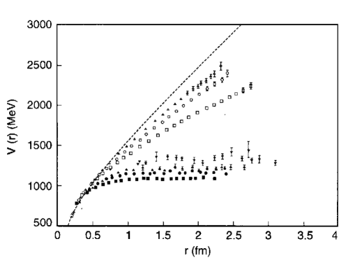
In recent years we have studied a generalized version of the Nambu–Jona-Lasinio (NJL) model which includes a covariant model of Lorentz-vector confinement [1-5]. Extensive applications have been made in the study of light mesons, with particularly satisfactory results for the properties of the $\eta(547)$, $\eta^{\prime}(958)$ and their radial excitations [6]. Since the modifications of the confining potential at finite temperature have recently been obtained in lattice simulations of QCD [7-12] (see Fig. 1), we became interested in introducing that feature in our generalized NJL model, whose Lagrangian is

$${\cal L}= \bar{q}(i\hbox to0.0pt{\hbox to5.30904pt{\hfil/\hfil}\hss}\partial-m^{0})q+\frac{G_{S}}{2}\sum_{i=0}^{8}[(\bar{q}\lambda^{i}q)^{2}+(\bar{q}i\gamma_{5}\lambda^{i}q)^{2}]$$ (1.1)

$$-\frac{G_{V}}{2}\sum_{i=0}^{8}[(\bar{q}\lambda^{i}\gamma_{\mu}q)^{2}+(\bar{q}\lambda^{i}\gamma_{5}\gamma_{\mu}q)^{2}]$$

$$+\frac{G_{D}}{2}\{\det[\bar{q}(1+\gamma_{5})q]+\det[\bar{q}(1-\gamma_{5})q]\}$$

$$+{\cal L}_{conf}\,.$$

Here, the $\lambda^{i}(i=0,\cdots,8)$ are the Gell-Mann matrices, with $\lambda^{0}=\sqrt{2/3}\mathbf{\,1}$, $m^{0}=\mbox{diag}\,(m_{u}^{0},m_{d}^{0},m_{s}^{0})$ is a matrix of current quark masses and ${\cal L}_{conf}$ denotes our model of confinement.

Figure 1: A comparison of quenched (open symbols) and unquenched (filled symbols) results for the interquark potential at finite temperature [7]. The dotted line is the zero temperature quenched potential. Here, the symbols for $T=0.80T_{c}$ [open triangle], $T=0.88T_{c}$ [open circle], $T=0.94T_{c}$ [open square], represent the quenched results. The results with dynamical fermions are given at $T=0.68T_{c}$ [solid downward-pointing triangle], $T=0.80T_{c}$ [solid upward-pointing triangle], $T=0.88T_{c}$ [solid circle], and $T=0.94T_{c}$ [solid square].

The dependence of the constituent masses of the NJL model upon the density of nuclear matter has been studied in earlier work, where we also studied the deconfinement of light mesons with increasing matter density [13]. In that work we introduced some density dependence of the coupling constants of the model. However, that was not done in a systematic fashion. As we will see, in our study of the temperature dependence of the constituent masses, as well as in the calculation of temperature-dependent hadron masses, we introduce a temperature dependence of the coupling constants, which for $T=T_{c}$, represents a 17% reduction of the magnitude of these constants. Since the use of temperature-dependent coupling constants is a novel feature of our work, we provide some evidence that such temperature dependence is necessary to create a formalism that is consistent with what is known concerning QCD thermodynamics. This aspect of our work is discussed in the Appendix.

The organization of our work is as follows. In Section II we review our treatment of confinement in our generalized NJL model and describe the modification we introduce to specify the temperature dependence of our confining interaction. In Section III we discuss the calculation of the temperature dependence of the constituent masses of the up, down and strange quarks. In Section IV we describe how random-phase-approximation (RPA) calculations may be made to obtain the wave function amplitudes and masses of the light mesons. (We consider the properties of the $\pi$, $K$, $f_{0}$, $a_{0}$ and $K_{0}^{*}$ mesons and their radial excitations in this work.) In Section V we provide the results of our calculations of the meson spectra at finite temperature. Finally, Section VI contains some further discussion and conclusions.

II covariant lorentz-vector model of confinement

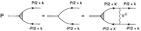
We have published a number of papers in which we have described our model of confinement[1-6]. In this work we provide a review of the important features of the model. As a first step, we introduce a vertex function for the confining interaction. [See Fig. 2.] For example, the vertex useful in the study of pseudoscalar mesons satisfies an equation of the form [6]

$$\overline{\Gamma}_{5,ab}(P,k) = \gamma_{5}-i\!\int\!\!\frac{d^{4}\!{k^{\,\prime}}}{(2\pi)^{4}}\,[\gamma^{\mu}S_{a}(P/2+k^{\,\prime})$$

$$\times\overline{\Gamma}_{5,ab}(P,k^{\,\prime})S_{b}(-P/2+k^{\,\prime})\gamma_{\mu}]V^{C}(\vec{k}-\vec{k}^{\prime})\,,$$

where $S_{a}(P/2+k^{\,\prime})=[\hbox to0.0pt{\hbox to7.80904pt{\hfil/\hfil}\hss}P/2+\hbox to0.0pt{\hbox to5.52084pt{\hfil/\hfil}\hss}k\,^{\prime}-m_{a}+i\eta]^{-1}$. Here, $m_{a}$ and $m_{b}$ are the constituent quark masses. We consider the form $V^{C}(r)=\kappa r\exp[-\mu r]$ and obtain the Fourier transform

$$V^{C}(\vec{k}-\vec{k}\,^{\prime})=-8\pi\kappa\left[\frac{1}{[(\vec{k}-\vec{k}\,^{\prime})^{2}+\mu^{2}]^{2}}-\frac{4\mu^{2}}{[(\vec{k}-\vec{k}\,^{\prime})^{2}+\mu^{2}]^{3}}\right]\,,$$ (2.2)

which is used in Eq. (2.1). Note that the matrix form of the confining interaction is $\overline{V}\,{}^{C}(\vec{k}-\vec{k}\,^{\prime})=\gamma^{\mu}(1)V^{C}(\vec{k}-\vec{k}\,^{\prime})\gamma_{\mu}(2)$, since we are using Lorentz-vector confinement. The form of the potential may be made covariant by introducing the four-vectors

$$\hat{k}^{\mu}=k^{\mu}-\frac{(k\cdot P)P^{\mu}}{P^{2}}\,,$$ (2.3)

and

$$\hat{k}^{\prime\,\mu}=k^{\prime\,\mu}-\frac{(k^{\prime}\cdot P)P^{\mu}}{P^{2}}\,.$$ (2.4)

We then define

$$V^{C}(\hat{k}-\hat{k}\,^{\prime})=-8\pi\kappa\left[\frac{1}{[-(\hat{k}-\hat{k}\,^{\prime})^{2}+\mu^{2}]^{2}}-\frac{4\mu^{2}}{[-(\hat{k}-\hat{k}\,^{\prime})^{2}+\mu^{2}]^{3}}\right]\,,$$ (2.5)

which reduces to $V^{C}(\vec{k}-\vec{k}\,^{\prime})$ of Eq. (2.2) in the meson rest frame, where $\vec{P}=0$.

Figure 2: The figure provides a schematic representation of Eq. (2.1) for the confining vertex function $\overline{\Gamma}_{5,ab}(P,k)$.

It is also useful to define scalar functions $\Gamma_{5,ab}^{+-}(P,k)$ and $\Gamma_{5,ab}^{-+}(P,k)$ [6]. We introduce

$$\Lambda_{a}^{(+)}(\vec{k})=\frac{\hbox to0.0pt{\hbox to5.52084pt{\hfil/\hfil}\hss}k_{a}+m_{a}}{2m_{a}}$$ (2.6)

and

$$\Lambda_{a}^{(-)}(-\vec{k})=\frac{\hbox to0.0pt{\hbox to5.55557pt{\hfil/\hfil}\hss}\widetilde{k}_{a}+m_{a}}{2m_{a}}\,,$$ (2.7)

where $k^{\mu}=[E_{a}(\vec{k}),\vec{k}]$ and $\widetilde{k}^{\mu}=[-E_{a}(\vec{k}),\vec{k}]$, and define

$$\Lambda_{a}^{(+)}(\vec{k})\overline{\Gamma}_{5,ab}(P,k)\Lambda_{b}^{(-)}(-\vec{k})=\Gamma_{5,ab}^{+-}(P,k)\Lambda_{a}^{(+)}(\vec{k})\gamma_{5}\Lambda_{b}^{(-)}(-\vec{k})\,,$$ (2.8)

and

$$\Lambda_{a}^{(-)}(-\vec{k})\overline{\Gamma}_{5,ab}(P,k)\Lambda_{b}^{(+)}(\vec{k})=\Gamma_{5,ab}^{-+}(P,k)\Lambda_{a}^{(-)}(-\vec{k})\gamma_{5}\Lambda_{b}^{(+)}(\vec{k})\,.$$ (2.9)

We have obtained equations for $\Gamma_{5}^{+-}(P,k)$ and $\Gamma_{5}^{-+}(P,k)$. For example, with $m_{a}=m_{b}$, we have

$$\Gamma_{5}^{+-}(P^{0},|\vec{k}|)=1-\!\int\!\!\frac{d^{3}\!{k^{\,\prime}}}{(2\pi)^{3}}\,\left[\frac{m^{2}-2E(\vec{k})E(\vec{k}\,^{\prime})}{E(\vec{k})E(\vec{k}\,^{\prime})}\right]\frac{\Gamma_{5}^{+-}(P^{0},|\vec{k}\,^{\prime}|)V^{C}(\vec{k}-\vec{k}\,^{\prime})}{P^{0}-2E(\vec{k}\,^{\prime})}\,.$$ (2.10)

Note that $\Gamma_{5}^{+-}(P^{0},|\vec{k}\,^{\prime}|)=0$, when $P^{0}=2E(\vec{k}\,^{\prime})$, so that one need not introduce a small quantity, $i\epsilon$, in the denominator on the right-hand side of Eq. (2.10). (Alternatively, we may note that $\Gamma_{5}^{+-}(P^{0},|\vec{k}|)=0$ when the quark and antiquark in Fig. 2 are on mass shell.) The confinement vertex functions defined in our work may be used to calculate vacuum polarization functions which are real functions. The unitarity cut, that would otherwise be present, is eliminated by the vertex functions which vanish when both the quark and antiquark go on mass shell [1-6].

We have presented Eq. (2.10), since we wish to stress that for the study of light mesons the constituent quark mass, $m$, is of the order of $|\vec{k}|$, so that $|\vec{k}|/m$ is not small. Therefore, the term in the square bracket on the right-hand side of Eq. (2.10), which would be equal to $-1$ in the nonrelativistic limit, provides quite important relativistic corrections to the form given in Eq. (2.5).

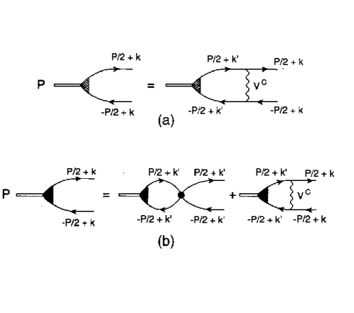
In Fig. 3a we show the homogeneous equation for the confining vertex. The solution of the homogeneous equation allows us to construct the wave functions bound in the confining field. For example, we may define

$$\psi_{i}^{(+)}(k)=\frac{\Gamma_{5}^{+-}(P_{i}^{0},k)}{P_{i}^{0}-2E(\vec{k})}$$ (2.11)

and

$$\psi_{i}^{(-)}(k)=-\frac{\Gamma_{5}^{-+}(-P_{i}^{0},k)}{P_{i}^{0}+2E(\vec{k})}\,,$$ (2.12)

which we may term the “large” and “small” components of the wave function of the bound state with energy $P_{i}^{0}$. In Fig. 3b we show the equation for the vertex function that includes both the effects of the short-range NJL interaction and the confining interaction. We will return to a consideration of the equations obtained in an analysis of Fig. 3b in Section IV where we consider the RPA equations of our model.

Figure 3: a) Bound states in the confining field (wavy line) may be found by solving the equation for the vertex shown in this figure, b) Effects of both the confining field and the short-range NJL interaction (filled circle) are included when solving for the vertex shown in this figure.

In order to motivate our treatment of the temperature dependence of the confining interaction, we have presented some results obtained with dynamical quarks (filled symbols) in Fig. 1. The fact that the potential becomes (approximately) constant for $r>1$ fm is ascribed to “string breaking” in the presence of dynamical quarks. (Note that, upon string breaking, the force between the infinitely massive quark and antiquark vanishes.)

For our calculations we have used $\mu=0.010$ GeV and $\kappa=0.055$ GeV² in the past. In order to introduce temperature dependence in our model, we replace $V^{C}(r)=\kappa r\exp[-\mu r]$ by $V^{C}(r,T)=\kappa r\exp[-\mu(T)r]$, with

$$\mu(T)=\frac{\mu_{0}}{1-0.7(T/T_{c})^{2}}\,,$$ (2.13)

where $\mu_{0}=0.01$ GeV. Values of $V^{C}(r,T)$ for various values of the ratio $T/T_{c}$ are given in Fig. 4. We remark that, while $V^{C}(r)\rightarrow 0$ for large $r$, the bound-state solutions found for $V^{C}(r)$ are largely unaffected, since barrier penetration effects are extremely small in our model. The maximum value of the potential is $V_{max}^{C}=\kappa/\mu e$ with the corresponding value of $r_{max}=1/\mu$. Thus, in the study of the bound states, our model is essentially equivalent to one with $V^{C}(r)=\kappa r\exp[-\mu r]$ for $r<r_{max}$ and $V^{C}(r)=V_{max}^{C}$ for $r>r_{max}$. The same remarks pertain, if we replace $\mu$ by $\mu(T)$ of Eq. (2.13). With that replacement, we have

$$V_{max}(T)=\frac{\kappa[1-0.7(T/T_{c})^{2}]}{\mu_{0}e}\,.$$ (2.14)

We note that $V_{max}$ is finite at $T=T_{c}$ , a result that is in general accord with what is found in lattice calculations of the interquark potential for massive quarks.

Figure 4: The potential $V^{C}(r,T)$ is shown for $T/T_{c}=0$ [solid line], $T/T_{c}=0.4$ [dotted line], $T/T_{c}=0.6$ [dashed line], $T/T_{c}=0.8$ [dash-dot line], $T/T_{c}=0.9$ [short dashes], $T/T_{c}=1.0$ [dash-dot-dot line]. Here, $V^{C}(r,T)=\kappa r\exp[-\mu(T)r]$, with $\mu(T)=0.01\mbox{GeV}/[1-0.7(T/T_{c})^{2}]$.

III calculation of constituent quark masses at finite temperature

In an earlier work we carried out a Euclidean-space calculation of the up, down, and strange constituent quark masses taking into account the ’t Hooft interaction and our confining interaction [14]. The ’t Hooft interaction plays only a minor role in the coupling of the equations for the constituent masses. If we neglect the confining interaction and the ’t Hooft interaction in the mean field calculation of the constituent masses, we can compensate for their absence by making a modest change in the value of $G_{S}$. [See Eq. (1.1).] For the calculations of this work we calculate the meson masses using the formalism presented in the Klevansky review [15]. (Note that our value of $G_{S}$ is twice the value of $G$ used in that review.) The relevant equation is Eq. (5.38) of Ref. [15]. Here, we put $\mu=0$ and write

$$m(T)=m^{0}+4GN_{C}\frac{m(T)}{\pi^{2}}\int_{0}^{\Lambda}dp\frac{p^{2}}{E_{p}}\tanh(\frac{1}{2}\beta E_{p})\,,$$ (3.1)

where $\Lambda=0.631$ GeV is a cutoff for the momentum integral, $\beta=1/T$ and $E_{p}=[\vec{p}^{2}+m^{2}(T)]^{1/2}$. In our calculations we replace $G$ by $G_{S}(T)/2$ and solve the equation

$$m(T)=m^{0}+2G_{S}(T)N_{C}\frac{m(T)}{\pi^{2}}\int_{0}^{\Lambda}dp\frac{p^{2}}{E_{p}}\tanh(\frac{1}{2}\beta E_{p})\,,$$ (3.2)

with $G_{S}(T)=11.38[1-0.17\,T/T_{c}]$ GeV, $m_{u}^{0}=0.0055$ GeV and $m_{s}^{0}=0.120$ GeV. Thus, we see that $G_{S}(T)$ is reduced from the value $G_{S}(0)$ by 17% when $T=T_{c}$. The results obtained in this manner for $m_{u}(T)$ and $m_{s}(T)$ are shown in Fig. 5. Here, the temperature dependence we have introduced for $G_{S}(T)$ serves to provide a somewhat more rapid restoration of chiral symmetry than that which is found for a constant value of $G_{S}$. That feature and the temperature dependence of the confining field leads to the deconfinement of the light mesons considered here at $T=T_{c}$. (See Section V.)

Figure 5: Temperature dependent constituent mass values, $m_{u}(T)$ and $m_{s}(T)$, calculated using Eq. (3.2) are shown. Here $m_{u}^{0}=0.0055$ GeV, $m_{s}^{0}=0.120$ GeV, and $G(T)=5.691[1-0.17(T/T_{c})]$, if we use Klevansky’s notation [15]. (The value of $G_{S}$ of Eq. (1.1) is twice the value of $G$ used in Ref. [15]).

IV random phase approximation calculations for meson masses at finite temperature

The analysis of the diagrams of Fig. 3b gives rise to a set of equations for various vertex functions. These equations are of the form of relativistic random-phase-approximation equations. The derivation of these equations for pseudoscalar mesons is given in Ref. [6], where we discuss the equations for pionic, kaonic and eta mesons. The equations for the eta mesons are the most complicated, since we consider singlet-octet mixing as well as pseudoscalar–axial-vector mixing. In that case there are eight vertex functions to consider, $\Gamma_{P,0}^{+-}$, $\Gamma_{A,0}^{+-}$, $\Gamma_{P,8}^{+-}$, $\Gamma_{A,8}^{+-}$, $\Gamma_{P,0}^{-+}$, $\Gamma_{A,0}^{-+}$, $\Gamma_{P,8}^{-+}$, $\Gamma_{A,8}^{-+}$, where $P$ refers to the $\gamma_{5}$ vertex and $A$ refers to the $\gamma_{0}\gamma_{5}$ vertex, which mixes with the $\gamma_{5}$ vertex. Corresponding to the eight vertex functions one may define eight wave function amplitudes [6].

The simplest example of our RPA calculations is that of the $a_{0}$ mesons, where there are only two vertex functions $\Gamma_{S}^{+-}$ and $\Gamma_{S}^{-+}$ to be calculated [4]. Associated with $\Gamma_{S}^{+-}$ and $\Gamma_{S}^{-+}$ are two wave functions $\phi_{S}^{+}$ and $\phi_{S}^{-}$, which are the large and small components respectively. In vacuum one has coupled equations for these wave functions.

$$2E_{u}(k)\phi^{+}(k)+\int\!dk^{\,\prime}\,[H_{C}(k,k^{\,\prime})+H_{NJL}(k,k^{\,\prime})]\phi^{+}(k^{\,\prime})$$ (4.1)

$$+\int\!dk^{\,\prime}\,H_{NJL}(k,k^{\,\prime})\phi^{-}(k^{\,\prime})=P^{0}\phi^{+}(k)\,,$$

$$-2E_{u}(k)\phi^{-}(k)-\int\!dk^{\,\prime}\,[H_{C}(k,k^{\,\prime})+H_{NJL}(k,k^{\,\prime})]\phi^{-}(k^{\,\prime})$$ (4.2)

$$-\int\!dk^{\,\prime}\,H_{NJL}(k,k^{\,\prime})\phi^{+}(k^{\,\prime})=P^{0}\phi^{-}(k)\,,$$

where $E_{u}(k)=[\vec{k}\,{}^{2}+m_{u}^{2}]^{1/2}$,

$$H_{C}(k,k^{\,\prime})=-\frac{1}{(2\pi)^{2}}\frac{[2V_{0}^{C}(k,k^{\,\prime})k^{2}k^{\,\prime\,2}+m_{u}^{2}kk^{\,\prime}V_{1}^{C}(k,k^{\,\prime})]}{E_{u}(k)E_{u}(k^{\,\prime})}\,,$$ (4.3)

and

$$H_{NJL}=\frac{8N_{c}}{(2\pi)^{2}}\frac{k^{2}k^{\,\prime\,2}G_{a_{0}}e^{-k^{2}/2\alpha^{2}}e^{-k^{\,\prime\,2}/2\alpha^{2}}}{E_{u}(k)E_{u}(k^{\,\prime})}\,.$$ (4.4)

In Eq. (4.4), $G_{a_{0}}$ is the effective coupling constant for the $a_{0}$ mesons, which depends upon the values of $G_{S}$, $G_{D}$ and the vacuum condensates. These relations for the various coupling constants, $G_{a_{0}}$, $G_{\pi}$, $G_{K}$, $G_{f_{0}}$, $G_{K_{0}^{*}}$, etc. may be found in Ref. [16]. In Eq. (4.3) we have introduced

$$V_{l}^{C}(k,k^{\,\prime})=\int_{-1}^{1}\!dx\,P_{l}(x)V^{C}(\vec{k}-\vec{k}{}^{\prime})\,.$$ (4.5)

Here, $x=\mbox{cos}\theta$ and $P_{l}(x)$ is a Legendre function. The terms exp[$-k^{2}/2\alpha^{2}$] and exp[$-k^{\,\prime\,2}/2\alpha^{2}$] are regulators with $\alpha=0.605$ GeV.

In order to solve these equations at finite temperature, we replace $m_{u}$, $G_{a_{0}}$ and $\mu_{0}$ by $m_{u}(T)$, $G_{a_{0}}(T)$ and $\mu(T)$. The values of $m(T)$ are given in Fig. 5, and we recall that $\mu(T)=\mu_{0}/[1-0.7(T/T_{c})^{2}]$. In the RPA, the solutions of Eqs. (4.1) and (4.2) come in pairs. For a state of energy $P_{i}^{0}$ there is another state with energy $-P_{i}^{0}$. Since the RPA Hamiltonian is not Hermitian, it is possible to obtain imaginary values for the energy. That is a signal of the instability of the ground state of the theory and requires that the problem be reformulated to obtain a stable ground state. This problem does not arise in the calculations reported in this work. In particular, the use of the temperature-dependent values of $G_{\pi}(T)$ avoids the appearance of pion condensation in the formalism.

V results of numerical calculations of meson masses at
finite temperature

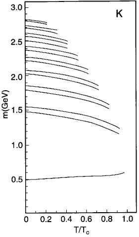
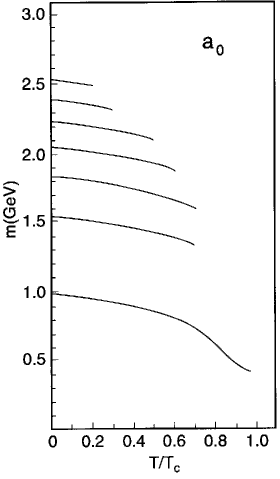
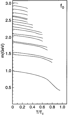
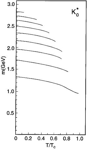
As noted earlier, the RPA equations for the $a_{0}$ mesons are given in Ref. [4] and those for the $\pi$, $K$ and $\eta$ mesons are given in Ref. [6]. The equations needed in the study of the $f_{0}$ mesons are to be found in Ref. [5], while the RPA equations for the study of the $K_{0}^{*}$ mesons are to be found in the Appendix of Ref. [3]. In Figs. 6-10 we present our results for the $\pi$, $K$, $a_{0}$, $f_{0}$ and $K_{0}^{*}$ mesons. The values of the coupling constants used are given in the figure captions. The reduction of the number of bound states with increasing temperature can be understood by noting that for the $\pi$ and $a_{0}$ mesons the continuum of the model lies above $V_{max}(T)+2m_{u}(T)$, while for the $K$ and $K_{0}^{*}$ mesons the continuum lies above $V_{max}(T)+m_{u}(T)+m_{s}(T)$. The situation is more complex in the case of the $f_{0}$ mesons which contain both $s\bar{s}$, $u\bar{u}$ and $d\bar{d}$ components. The bound states lie below the $s\bar{s}$ continuum which begins at $V_{max}(T)+2m_{s}(T)$. However, we note that the absence of bound states at $T=T_{c}$ for all the mesons considered here is due to the reduction of the value of the confining potential and of the constituent quark masses.

It is of interest to note that the mass values of the $a_{0}$ and $f_{0}$ mesons tend toward degeneracy with the pion as $T\rightarrow T_{c}$ . However, the mesons disassociate before a greater degeneracy is achieved. That is in contrast to the results obtained in the SU(2) formalism considered by Hatsuda and Kunihiro [16]. Since these authors do not include a model of the confinement-deconfinement transition, they are able to see the approximate degeneracy of the sigma meson and the pion with increasing temperature. It is also worth noting that in the SU(3) formalism the sigma meson is replaced by the $f_{0}(980)$ as the chiral partner of the pion.

Figure 6: The mass values of the pionic states calculated in this work with $G_{\pi}(T)=13.49[1-0.17\,T/T_{c}]$ GeV, $G_{V}(T)=11.46[1-0.17\,T/T_{c}]$ GeV, and the quark mass values given in Fig. 5. The value of the pion mass is 0.223 GeV at $T/T_{c}=0.90$, where $m_{u}(T)=0.102$ GeV and $m_{s}(T)=0.449$ GeV. The pion is bound up to $T/T_{c}=0.94$, but is absent beyond that value.

Figure 7: Mass values of kaonic states calculated with $G_{K}(T)=13.07[1-0.17\,T/T_{c}]$ GeV, $G_{V}(T)=11.46[1-0.17\,T/T_{c}]$ GeV, and the quark mass values given in Fig. 5. The value of the kaon mass is 0.598 GeV at $T/T_{c}=0.95$, where $m_{u}(T)=0.075$ GeV and $m_{s}(T)=0.439$ GeV.

Figure 8: Mass values for the $a_{0}$ mesons calculated with $G_{a_{0}}(T)=13.1[1-0.17\,T/T_{c}]$ GeV, and the quark mass values given in Fig. 5. The value of the $a_{0}$ mass at $T/T_{c}=0.95$ is 0.416 GeV.

Figure 9: Mass values of the $f_{0}$ mesons calculated with $G_{00}(T)=14.25[1-0.17\,T/T_{c}]$ GeV, $G_{88}(T)=10.65[1-0.17\,T/T_{c}]$ GeV, $G_{08}(T)=0.495[1-0.17\,T/T_{c}]$ GeV, and $G_{80}(T)=G_{08}(T)$ in a singlet-octet representation. The quark mass values used are shown in Fig. 5. The $f_{0}$ has a mass of 0.400 GeV at $T/T_{c}=0.95$.

Figure 10: Mass values obtained for the $K_{0}^{*}$ mesons with $G_{K_{0}^{*}}(T)=10.25[1-0.17\,T/T_{c}]$ GeV, and the quark mass values shown in Fig. 5.

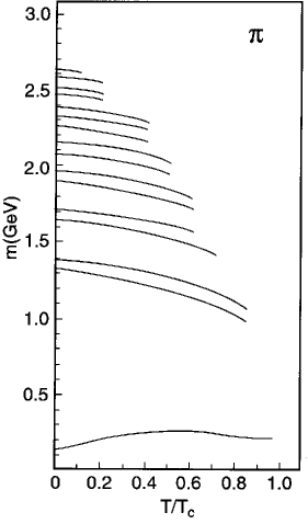
In order to demonstrate the interplay of chiral symmetry restoration and dissolution of our meson states, we have performed calculations in which the quark masses are unchanged from their value at $T=0$. For the pion, with $m_{u}=m_{d}=0.364$ GeV and for $T/T_{c}=0.95$, we find bound states at 0.530, 1.242 and 1.305 GeV. If we also consider the values of the coupling constants and quark masses fixed at their $T=0$ values, bound states are found at 0.102, 2.248 and 1.298 GeV when $T/T_{c}=0.95$. A similar analysis for the kaon states yields bound states at $T=T_{c}$ of 0.738, 1.395 and 1.444 GeV, if we put $m_{u}=0.364$ GeV and $m_{s}=0.565$ GeV. If, in addition, we neglect the temperature dependence of the coupling constants, we have bound kaon states at 0.482, 1.440 and 1.439 GeV.

In the case of the $a_{0}$ states, putting $m_{u}=m_{d}=0.364$ GeV yields a single state at 0.960 GeV at $T=T_{c}$ , if we neglect the temperature dependence of the coupling constant. If we maintain the temperature dependence of the coupling constant, we find a single state at 1.067 GeV, if the quark masses are kept at their $T=0$ values.

From this analysis, we see that the reduction of the quark masses with increasing temperature, which represents a partial restoration of chiral symmetry, is an essential feature of our model. In the past, lattice simulations of QCD have indicated that deconfinement and restoration of chiral symmetry take place at the same temperature. Since our Lagrangian contains current quark masses for the up, down and strange quarks, chiral symmetry is not completely restored at the higher temperatures in our model. However, the model does exhibit quite significant reductions of the up and down constituent quark masses for $T\gtrsim T_{c}$ (See Fig. 5), so that deconfinement is here associated with a significant restoration of chiral symmetry.

VI discussion

In recent years we have seen extensive applications of the NJL model in the study of matter at high density [17-21]. There is great interest in the diquark condensates and color superconductivity predicted by the NJL model and closely related models that are based upon instanton dynamics. It is noted by workers in this field that the NJL model does not describe confinement, with the consequence that one can not present a proper description of the hadronic phase that exists at the smaller values of the temperature and density in the QCD phase diagram. Thus, the attitude adopted is that, if one works in the deconfined phase, the NJL model may provide a satisfactory description of the quark interaction. In the present work we have modified the NJL model so that we can describe light mesons and their radial excitations, as well as the confinement-deconfinement transition at $T=T_{c}$ . In an earlier work we studied the confinement-deconfinement transition for finite matter density at $T=0$ [13]. (A more comprehensive study would include both finite temperature and finite density.) As in the present work, in which we introduced a temperature-dependent coupling constants, we used density-dependent coupling constants in Ref. [13]. If such dependence exists, it would have important consequences for the study of dense matter using the NJL model.

One interesting feature of our results is that both the lowest $a_{0}$ and $f_{0}$ states move toward degeneracy with the pion as the temperature is increased. However, the system is deconfined before such degeneracy can be exhibited.

We stress that the restoration of chiral symmetry is intimately connected with the dissolution of our meson states at $T=T_{c}$ . As we saw in the discussion toward the end of Section V, the various mesons studied here still have bound states at $T=T_{c}$ , if only the temperature dependence of the confining field is included in the model.

The behavior of charmonium across the deconfinement transition has recently been studied using lattice simulations of QCD [22]. The authors of Ref. [22] point out that, unlike the case of light mesons, charmonia may exist as bound states even after the deconfinement transition. They state:“Our studies support the sequential pattern for charmonium dissolution obtained from potential model studies, where the broader bound states (the scalar and axial vector channels) dissolve before the pseudoscalar and vector channels [23]. The pseudoscalar and vector channels are seen to survive as bound states still at 1.25$T_{c}$ and probably dissolve after 1.5$T_{c}$ .”

*

Appendix A

Since the introduction of temperature-dependent coupling constants for the NJL model is a novel feature of our work, we provide arguments in this Appendix to justify their introduction. We make reference to Fig. 1.3 of Ref. [24]. That figure shows the behavior of the ratio $\epsilon/T^{4}$ and $3P/T^{4}$ for the pure gauge sector of QCD. Here $\epsilon$ is the energy density and $P$ is the pressure. Ideal gas behavior implies $\epsilon=3P$. The values of $\epsilon/T^{4}$ and $3P/T^{4}$ are compared to the value $\epsilon_{SB}/T^{4}=8\pi^{2}/15$ for an ideal gluon gas. It may be seen from the figure that at $T=3T_{c}$ there are still significant differences from the ideal gluon gas result. Deviations from ideal gas behavior become progressively smaller with increasing $T/T_{c}$ and could be considered to be relatively unimportant for $T/T_{c}>5$.

To provide evidence for temperature-dependent coupling constants, we discuss the calculation of hadronic current correlators in the deconfined phase. The procedure we adopt is based upon the real-time finite-temperature formalism, in which the imaginary part of the polarization function may be calculated. Then, the real part of the function is obtained using a dispersion relation. The result we need for this work has been already given in the work of Kobes and Semenoff [25]. (In Ref. [25] the quark momentum is $k$ and the antiquark momentum is $k-P$. We will adopt that notation in this section for ease of reference to the results presented in Ref. [25].) With reference to Eq. (5.4) of Ref. [25], we write the imaginary part of the scalar polarization function as

$$\mbox{Im}\,J^{S}(P^{2},T)=\frac{1}{2}(2N_{c})\beta_{S}\,\epsilon(p^{0})\!\int\!\!\frac{d^{3}\!{k}}{(2\pi)^{3}}\,e^{-\vec{k}\,{}^{2}/\alpha^{2}}\left(\frac{2\pi}{2E_{1}(k)2E_{2}(k)}\right)$$ (A1)

$$\{(1-n_{1}(k)-n_{2}(k))\delta(p^{0}-E_{1}(k)-E_{2}(k))$$

$$-(n_{1}(k)-n_{2}(k))\delta(p^{0}+E_{1}(k)-E_{2}(k))$$

$$-(n_{2}(k)-n_{1}(k))\delta(p^{0}-E_{1}(k)+E_{2}(k))$$

$$-(1-n_{1}(k)-n_{2}(k))\delta(p^{0}+E_{1}(k)+E_{2}(k))\}\,.$$

Here, $E_{1}(k)=[\vec{k}\,{}^{2}+m_{1}^{2}(T)]^{1/2}$. Relative to Eq. (5.4) of Ref. [25], we have changed the sign, removed a factor of $g^{2}$ and have included a statistical factor of $2N_{c}$, where the factor of 2 arises from the flavor trace. In addition, we have included a Gaussian regulator, $\exp[-\vec{k}\,{}^{2}/\alpha^{2}]$, with $\alpha=0.605$ GeV, which is the same as that used in most of our applications of the NJL model in the calculation of meson properties. We also note that

$$n_{1}(k)=\frac{1}{e^{\,\beta E_{1}(k)}+1}\,,$$ (A2)

and

$$n_{2}(k)=\frac{1}{e^{\,\beta E_{2}(k)}+1}\,.$$ (A3)

For the calculation of the imaginary part of the polarization function, we may put $k^{2}=m_{1}^{2}(T)$ and $(k-p)^{2}=m_{2}^{2}(T)$, since in that calculation the quark and antiquark are on-mass-shell. We will first remark upon the calculation of scalar correlators [25]. In that case, the factor $\beta_{S}$ in Eq. (A1) arises from a trace involving Dirac matrices, such that

$$\beta_{S} = -\mbox{Tr}[(\hbox to0.0pt{\hbox to5.52084pt{\hfil/\hfil}\hss}k+m_{1})(\hbox to0.0pt{\hbox to5.52084pt{\hfil/\hfil}\hss}k-\hbox to0.0pt{\hbox to7.80904pt{\hfil/\hfil}\hss}P+m_{2})]$$ (A4)

$$= 2P^{2}-2(m_{1}+m_{2})^{2}\,,$$ (A5)

where $m_{1}$ and $m_{2}$ depend upon temperature. In the frame where $\vec{P}=0$, and in the case $m_{1}=m_{2}$, we have $\beta_{S}=2P_{0}^{2}(1-{4m^{2}}/{P_{0}^{2}})$. For the scalar case, with $m_{1}=m_{2}$, we find

$$\mbox{Im}\,J^{S}(P^{2},T)=\frac{N_{c}P_{0}^{2}}{4\pi}\left(1-\frac{4m^{2}}{P_{0}^{2}}\right)^{3/2}e^{-\vec{k}\,{}^{2}/\alpha^{2}}[1-2n_{1}(k)]\,,$$ (A6)

where

$$\vec{k}\,{}^{2}=\frac{P_{0}^{2}}{4}-m^{2}(T)\,.$$ (A7)

We may evaluate Eq. (2.8) for $m(T)=m_{u}(T)=m_{d}(T)$ and define $\mbox{Im}\,J_{u}^{S}(P^{2},T)$. Then we put $m(T)=m_{s}(T)$, we define $\mbox{Im}\,J_{s}^{S}(P^{2},T)$. These two functions are needed for a calculation of the scalar-isoscalar correlator. The real parts of the functions $J_{u}^{S}(P^{2},T)$ and $J_{s}^{S}(P^{2},T)$ may be obtained using a dispersion relation, as noted earlier.

For pseudoscalar mesons, we replace $\beta_{S}$ by

$$\beta_{P} = -\mbox{Tr}[i\gamma_{5}(\hbox to0.0pt{\hbox to5.52084pt{\hfil/\hfil}\hss}k+m_{1})i\gamma_{5}(\hbox to0.0pt{\hbox to5.52084pt{\hfil/\hfil}\hss}k-\hbox to0.0pt{\hbox to7.80904pt{\hfil/\hfil}\hss}P+m_{2})]$$ (A8)

$$= 2P^{2}-2(m_{1}-m_{2})^{2}\,,$$ (A9)

which for $m_{1}=m_{2}$ is $\beta_{P}=2P_{0}^{2}$ in the frame where $\vec{P}=0$. We find, for the $\pi$ mesons,

$$\mbox{Im}\,J^{P}(P^{2},T)=\frac{N_{c}P_{0}^{2}}{4\pi}\left(1-\frac{4m(T)^{2}}{P_{0}^{2}}\right)^{1/2}e^{-\vec{k}\,{}^{2}/\alpha^{2}}[1-2n_{1}(k)]\,,$$ (A10)

where $\vec{k}\,{}^{2}={P_{0}^{2}}/4-m_{u}^{2}(T)$, as above. Thus, we see that, relative to the scalar case, the phase space factor has an exponent of 1/2 corresponding to a s-wave amplitude, rather than the p-wave amplitude of scalar mesons. For the scalars, the exponent of the phase-space factor is 3/2, as seen in Eq. (A6).

For a study of vector mesons we consider

$$\beta_{\mu\nu}^{V}=\mbox{Tr}[\gamma_{\mu}(\hbox to0.0pt{\hbox to5.52084pt{\hfil/\hfil}\hss}k+m_{1})\gamma_{\nu}(\hbox to0.0pt{\hbox to5.52084pt{\hfil/\hfil}\hss}k-\hbox to0.0pt{\hbox to7.80904pt{\hfil/\hfil}\hss}P+m_{2})]\,,$$ (A11)

and calculate

$$g^{\mu\nu}\beta_{\mu\nu}^{V}=4[P^{2}-m_{1}^{2}-m_{2}^{2}+4m_{1}m_{2}]\,,$$ (A12)

which, in the equal-mass case, is equal to $4P_{0}^{2}+8m^{2}(T)$, when $m_{1}=m_{2}$ and $\vec{P}=0$. Note that for the elevated temperatures considered in this work $m_{u}(T)=m_{d}(T)$ is quite small, so that $4P_{0}^{2}+8m_{u}^{2}(T)$ can be approximated by $4P_{0}^{2}$ when we consider the $\rho$ meson.

We now consider the calculation of temperature-dependent hadronic current correlation functions. The general form of the correlator is a transform of a time-ordered product of currents,

$$C(P^{2},T)=i\int d^{4}xe^{\,ip\cdot x}<<\mbox{T}(j(x)j(0)>>\,,$$ (A13)

where the double bracket is a reminder that we are considering the finite temperature case.

For the study of pseudoscalar states, we may consider currents of the form $j_{P,\,i}(x)=\bar{q}(x)i\gamma_{5}\lambda^{i}q(x)$, where, in the case of the $\pi$ mesons, $i=1,2,$ and 3. For the study of pseudoscalar-isoscalar mesons, we again introduce $j_{P,\,i}(x)=\bar{q}(x)\lambda^{i}q(x)$, but here $i=0$ for the flavor-singlet current and $i=8$ for the flavor-octet current.

In the case of the $\pi$ mesons, the correlator may be expressed in terms of the basic vacuum polarization function of the NJL model, $J_{P}(P^{2},T)$. Thus,

$$C_{\pi}(P^{2},T)=J_{P}(P^{2},T)\frac{1}{1-G_{\pi}(T)J_{P}(P^{2},T)}\,,$$ (A14)

where $G_{\pi}(T)$ is the coupling constant appropriate for our study of the $\pi$ mesons. We have found $G_{\pi}(0)=13.49$ GeV^-2 by fitting the pion mass in a calculation made at $T=0$, with $m_{u}=m_{d}=0.364$ GeV.

The calculation of the correlator for pseudoscalar-isoscalar states is more complex, since there are both flavor-singlet and flavor-octet states to consider. We may define polarization functions for $u$, $d$ and $s$ quarks: $J_{u}(P^{2},T)$, $J_{d}(P^{2},T)$ and $J_{s}(P^{2},T)$. In terms of these polarization functions we may then define

$$J_{00}(P^{2},T)=\frac{2}{3}[J_{u}(P^{2},T)+J_{d}(P^{2},T)+J_{s}(P^{2},T)]\,,$$ (A15)

$$J_{08}(P^{2},T)=\frac{\sqrt{2}}{3}[J_{u}(P^{2},T)+J_{d}(P^{2},T)-2J_{s}(P^{2},T)]\,,$$ (A16)

and

$$J_{88}(P^{2},T)=\frac{1}{3}[J_{u}(P^{2},T)+J_{d}(P^{2},T)+4J_{s}(P^{2},T)]\,.$$ (A17)

We also introduce the matrices

$$J(P^{2},T)=\left[\begin{array}[]{cc}J_{00}(P^{2},T)&J_{08}(P^{2},T)\\ J_{80}(P^{2},T)&J_{88}(P^{2},T)\end{array}\right]\,,$$ (A20)

$$G(T)=\left[\begin{array}[]{cc}G_{00}(T)&G_{08}(T)\\ G_{80}(T)&G_{88}(T)\end{array}\right]\,,$$ (A23)

and

$$C(P^{2},T)=\left[\begin{array}[]{cc}C_{00}(P^{2},T)&C_{08}(P^{2},T)\\ C_{80}(P^{2},T)&C_{88}(P^{2},T)\end{array}\right]\,.$$ (A26)

We then write the matrix relation

$$C(P^{2},T)=J(P^{2},T)[1-G(T)J(P^{2},T)]^{-1}\,.$$ (A27)

The use of our energy-dependent coupling constants is meant to be consistent with the approach to asymptotic freedom at high temperature. In order to understand this feature in our model, we can calculate the correlator with constant values of $G_{00}$, $G_{88}$ and $G_{08}$ and also with $G_{00}(T)=G_{00}[1-0.17\,T/T_{c}]$, etc. (In this work we use $G_{00}=8.09$ GeV^-2, $G_{88}=13.02$ GeV^-2 and $G_{08}=-0.4953$ GeV^-2.)

We now consider the values of $\mbox{Im}\,C_{88}(P^{2})$ for $T/T_{c}=4.0$. In Fig. 11 we show the values of $\mbox{Im}\,C_{88}(P^{2})$ calculated in our model with temperature-dependent coupling parameters as a dashed line. The dotted line shows the values of the correlator for $G_{00}=G_{88}=G_{08}=0$, while the solid line shows the values when the coupling parameters are kept at their values at $T=0$. We see that we have resonant behavior in the case the parameters are temperature independent.

In Fig. 12 we show similar results for $T/T_{c}=5.88$. Here the temperature-dependent coupling constants are equal to zero, so that the lines corresponding to the dashed and dotted lines of Fig. 11 coincide. The solid line again shows resonant behavior at a value of $T/T_{c}$ where we expect only weak interactions associated with asymptotic freedom. We conclude that the model with constant values of the coupling parameters yields unacceptable results, while our model, which has temperature-dependent coupling parameters, behaves as one may expect, when the results of lattice simulations of QCD thermodynamics are taken into account.

Figure 11: The imaginary part of the correlator $C_{88}(P^{2})$ is shown for $T/T_{c}=4.0$. The dashed line is the result for the temperature-dependent coupling parameters of our model, while the solid line represents the results for coupling parameters kept at their $T=0$ values. The dotted line shows the values of the correlator when the coupling parameters are set equal to zero.

Figure 12: The imaginary part of the correlator $C_{88}(P^{2})$ is shown for $T/T_{c}=5.88$. [See caption to Fig. 11.] Here the dashed and dotted lines of Fig. 11 coincide.

References

- (1) C. M. Shakin and Huangsheng Wang, Phys. Rev. D 63 , 014019 (2000).
- (2) L. S. Celenza, Huangsheng Wang, and C. M. Shakin, Phys. Rev. C 63 , 025209 (2001).
- (3) C. M. Shakin and Huangsheng Wang, Phys. Rev. D 63 , 074017 (2001).
- (4) C. M. Shakin and Huangsheng Wang, Phys. Rev. D 63 , 114007 (2001).
- (5) C. M. Shakin and Huangsheng Wang, Phys. Rev. D 64 , 094020 (2001).
- (6) C. M. Shakin and Huangsheng Wang, Phys. Rev. D 65 , 094003 (2002).
- (7) C. DeTar, O. Kaczmarek, F. Karsch, and E. Laermann, Phys. Rev. D 59 , 031501 (1998).
- (8) H. D. Trottier, Phys. Rev. D 60 , 034506 (1999).
- (9) O. Kaczmarek, F. Karsch, and E. Laermann and M. Ltgemeier, Phys. Rev. D 62 , 034021 (2000).
- (10) B. Bolder et al., Phys. Rev. D 63 , 074504 (2001).
- (11) C. Bernard et al., Phys. Rev. D 64 , 074509 (2001).
- (12) A. Duncan, E. Eichten, and H. Thacker, Phys. Rev. D 63 , 111501(R) (2001).
- (13) Hu Li and C. M. Shakin, Phys. Rev. D 66, 074016 (2002).
- (14) Bing He, Hu Li, Qing Sun, and C. M. Shakin, nucl-th/0203010.
- (15) S. P. Klevansky, Rev. Mod. Phys. 64 , 649 (1992).
- (16) T. Hatsuda and T. Kunihiro, Phys. Rep. 247 , 221 (1994).
- (17) For reviews, see K. Rajagopal and F. Wilcek, in B. L. Ioffe Festscrift; At the Frontier of Particle Physics/Handbook of QCD, M. Shifman ed. (World Scientific, Singapore 2001); M. Alford, Annu. Rev. Nucl. Part. Sci. 51, 131 (2001).
- (18) M. Alford, R. Rajagopal and F. Wilcek, Phys. Lett. B 422 , 247 (1998).
- (19) R. Rapp, T. Schfer, E. V. Shuryak and M. Velkovsky, Phys. Rev. Lett. 81 , 53 (1998).
- (20) M. Alford, J. Berges and K. Rajagopal, Nucl. Phys. B 558 , 219 (1999).
- (21) J. Kundu and K. Rajagopal, Phys. Rev. D 65, 094022 (2002).
- (22) S. Datta, F. Karsck, P. Petreczky and I. Wetzorke, hep-lat/0208012.
- (23) S. Digal, P. Petreczky, and H. Satz, Phys. Rev. D 64 , 094015 (2001).
- (24) M. Le Bellac, Thermal Field Theory, (Cambridge Univ. Press, Cambridge, U.K., 1996).
- (25) R. L. Kobes and G. W. Semenoff, Nucl. Phys. B 260, 714 (1985).