1 Introduction

Why should we bother about radiative corrections to processes with supersymmetric (SUSY) particles when no SUSY particle has been found yet? Clearly, one expects that the next generation of high energy physics experiments at Tevatron, LHC, and at a future linear $e^{+}e^{-}$ collider will discover supersymmetric particles. But it is also obvious that precision studies are needed in order to single out the right supersymmetric model and to reconstruct its fundamental parameters. In particular, at a linear $e^{+}e^{-}$ collider it will be possible to perform measurements with high precision. For instance, at TESLA [1] the precision of the mass determination of charginos or neutralinos will be $\Delta m_{\tilde{\chi}^{\pm,0}}=0.1-1$ GeV and of sleptons (sneutrinos) $\Delta m_{\tilde{l},\tilde{\nu}}=0.05-3$ GeV. To match this accuracy, it is inevitable to include higher order corrections. Moreover, in some cases these corrections can be very large.

In the following we will discuss SUSY particle production in $e^{+}e^{-}$ colliders and SUSY particle decays within the Minimal Supersymmetric Standard Model (MSSM):

$$e^{+}e^{-} \rightarrow \tilde{\chi}^{+}_{i}\tilde{\chi}^{-}_{j}\hskip 85.35826pti,j=1,2$$

$$\rightarrow \tilde{\chi}^{0}_{l}\tilde{\chi}^{0}_{k}\hskip 89.05713ptl,k=1,\ldots,4$$

$$e^{+}e^{-} \rightarrow {\tilde{f}}_{i}\ \bar{\!\!\tilde{f}}_{\!\!j}\hskip 44.3863pt{\rm with}\hskip 36.98857ptf=l,q\;\;(q=b,t)$$ (2)

$$e^{+}e^{-} \rightarrow q\ \bar{\!\tilde{q}}\,\tilde{g}\,(g)\hskip 25.60747pt{\rm with\;light\;quarks}$$ (3)

and the decays

$${\tilde{f}}_{1,2} \rightarrow f\,\tilde{\chi}^{\pm}_{i}$$ (4)

$$\rightarrow f\,\tilde{\chi}^{0}_{l}$$

$${\tilde{f}}_{i} \rightarrow {\tilde{f}}_{j}+(W,Z,H_{m})\hskip 55.19832ptm=1,\ldots,4$$ (5)

$$H_{m} \rightarrow \tilde{\chi}_{i}^{+}\tilde{\chi}_{j}^{-},\;\tilde{\chi}_{l}^{0}\tilde{\chi}_{k}^{0}\hskip 31.29802pt{\rm or}\hskip 31.29802pt\tilde{\chi}^{+,\,0}_{i,\,k}\rightarrow\tilde{\chi}^{+,\,0}_{j,\,l}+H_{m}$$ (6)

$$H_{m} \rightarrow \tilde{q}_{i}\ \bar{\!\tilde{q}}_{\!j}$$ (7)

with $H_{m}=\{h^{0},H^{0},A^{0},H^{\pm}\}$. ${\tilde{f}}_{i}$ (with $i=1,2$) are the mass eigenstates of the sfermions.

For calculating higher order corrections, one has to employ appropriate renormalization conditions, or equivalently, one has to fix the counter terms for the SUSY parameters. We will discuss these fixings in the on–shell scheme. This method should of course preserve the symmetries (supersymmetry and gauge symmetry) and, if possible, should be process independent and lead to numerically stable results. We will take in the following the point of view of a practitioner, referring for a general discussion on the renormalization of the MSSM using an algebraic method to [2].

2 General Method

We start from the Lagrangian of the MSSM with its gauge–fixing and ghost part, without writing it explicitly:

$${\cal{L}}={\cal{L}}_{\rm MSSM}+{\cal{L}}_{\rm gauge\;fixing}+{\cal{L}}_{\rm ghost}.$$ (8)

We get the renormalized Lagrangian by transforming all fields by
$\phi_{i}\rightarrow\sqrt{Z_{i}}\phi_{i}=(1+{\frac{1}{2}}\delta{Z_{i}})\phi_{i}$ and all parameters, such as couplings, by $c_{k}\rightarrow c_{k}+\delta c_{k}$:

$${\cal{L}}^{\rm ren}={\cal{L}}-\delta{\cal{L}},$$ (9)

where ${\cal{L}}^{\rm ren}$ has the same form as ${\cal{L}}$, and $\delta{\cal{L}}$ is the counter term part which renders ${\cal{L}}^{\rm ren}$ finite. $\delta{\cal{L}}$ contains all counter terms to the parameters which have to be fixed appropriately. We will use here the $\overline{\rm DR}$ (dimensional reduction) scheme [3] with the dimension $n=4-r\epsilon$, $r=0$. It conserves supersymmetry at least up to one–loop. As already mentioned, we employ the on–shell scheme with the particle masses as pole masses and the parameters determined on–shell. As a consequence, there is no scale dependence. We also use the $R_{\xi}$ gauge [4].

2.1 Mixing angle of sfermions

The SUSY partners ${\tilde{f}}_{L}$, ${\tilde{f}}_{R}$ to the fermion $f$ mix with each other due to the SU(2)$\times$U(1) breaking. The mass eigenstates ${\tilde{f}}_{i}$, $i=1,2$ are

$${\tilde{f}}_{i}=R{\tilde{f}}_{\alpha},\hskip 85.35826pt\alpha=L,R$$

with $R=\left(\begin{array}[]{cc}\cos{\theta_{\tilde{f}}}&\sin{\theta_{\tilde{f}}}\\ -\sin{\theta_{\tilde{f}}}&\cos{\theta_{\tilde{f}}}\end{array}\right)$. The mixing angle $\theta_{\tilde{f}}$ is a measurable quantity.
The corresponding potential $V$ at tree–level is

$$V = \left({\tilde{f}}^{*}_{L},{\tilde{f}}^{*}_{R}\right)\underbrace{\left(\begin{array}[]{cc}m_{LL}^{2}&m_{LR}^{2}\\ m_{RL}^{2}&m_{RR}^{2}\end{array}\right)}_{\cal{M}}\left(\begin{array}[]{c}{\tilde{f}}_{L}\\ {\tilde{f}}_{R}\end{array}\right)\,+\,{\rm h.c.}$$ (14)

$$= {\tilde{f}}_{i}\left({\cal{M}}_{D}\right)_{ii}{\tilde{f}}_{i},\hskip 56.9055pt{\cal{M}}_{D}=R\,{\cal{M}}\,R^{\dagger}=\left(\begin{array}[]{cc}m_{{\tilde{f}}_{1}}^{2}&0\\ 0&m_{{\tilde{f}}_{2}}^{2}\end{array}\right)$$ (17)

It is renormalized by

$${\tilde{f}}_{i}^{0} = \left(1+{\frac{1}{2}}{Z}\right)\,{\tilde{f}}_{i}$$

$$R^{0} = R+\delta{R}=\left(1+\delta{r}\right)R$$

$${\cal{M}}^{0} = {\cal{M}}+\delta{\cal{M}}$$

First we observe that due to the unitarity of $R^{0}$ and $R$, $\delta{r}$ is antihermitian, $\delta{r}=-\delta{r}^{\dagger}$. On the other hand, one can decompose the wave–function renormalization counter term into a hermitian and antihermitian part:

$$\delta{Z}={\frac{1}{2}}\left(\delta{Z}+\delta{Z}^{\dagger}\right)+{\frac{1}{2}}\left(\delta{Z}-\delta{Z}^{\dagger}\right)\,,$$

It is therefore natural to fix $\delta{r}$ such that it cancels the antihermitian part of $\delta{Z}$, i.e.

$$\delta{R} = \frac{1}{4}\left[\delta{Z}^{\tilde{f}}-\left(\delta{Z}^{\tilde{f}}\right)^{\dagger}\right]R\,,$$

$$\delta\theta_{\tilde{f}} = \frac{1}{4}\left(\delta{Z}^{\tilde{f}}_{12}-\delta{Z}^{\tilde{f}}_{21}\right)~{}=~{}\frac{\Sigma_{12}\big{(}m_{{\tilde{f}}_{2}}^{2}\big{)}+\Sigma_{21}\big{(}m_{{\tilde{f}}_{1}}^{2}\big{)}}{2\Big{(}m_{{\tilde{f}}_{1}}^{2}-m_{{\tilde{f}}_{2}}^{2}\Big{)}}\,.$$ (18)

Here $\Sigma_{12}$ are the non-diagonal self–energies of ${\tilde{f}}_{i}$.
This is a process independent fixing nowadays conventionally used [5, 6]. This fixing is, however, in general gauge dependent. It was shown in [7] that this gauge dependence can be avoided or, equivalently the result in the $\xi=1$ gauge can be regarded as the gauge independent one.

The mixing angle $\alpha$ in the $h^{0}$–$H^{0}$ system can be treated in a similar way as above, leading to the counter term

$$\delta\alpha=\frac{1}{4}\left(\delta{Z}_{21}-\delta{Z}_{12}\right)\,,$$ (19)

where the index $1$ is for $h^{0}$ and $2$ for $H^{0}$.

2.2 Renormalization of the chargino mass matrix

Here we closely follow the method outlined in [8].
In the MSSM the chargino mass at tree–level is given by

$$X=\left(\begin{array}[]{cc}M&\sqrt{2}\,m_{W}\sin\beta\\ \sqrt{2}\,m_{W}\cos\beta&\mu\end{array}\right)\,.$$ (20)

It is diagonalized by the two real $(2\times 2)$ matrices $U$ and $V$:

$$U\,X\,V^{T}=M_{D}=\left(\begin{array}[]{cc}m_{\tilde{\chi}^{+}_{1}}&0\\ 0&m_{\tilde{\chi}^{+}_{2}}\end{array}\right)\,,$$ (21)

with $m_{\tilde{\chi}^{+}_{1}}$ and $m_{\tilde{\chi}^{+}_{2}}$ the physical masses of the charginos (choosing $m_{\tilde{\chi}^{+}_{1}}<m_{\tilde{\chi}^{+}_{2}}$) where

$$\chi^{L}_{i}=V_{ij}\,\psi^{L}_{j}\,,\hskip 42.67912pt\chi^{R}_{i}=U_{ij}\,\psi^{R}_{j}\,,\hskip 71.13188pti=1,2\,,$$

forming the Dirac spinor

$${\tilde{\chi}}^{+}_{i}=\left(\begin{array}[]{c}\chi_{i}^{L}\\ \bar{\chi}_{i}^{R}\end{array}\right)\,.$$

Then we renormalize by performing the shifts

$$X^{0} = X+\delta X\,,$$

$$U^{0} = U+\delta U\,,$$

$$V^{0} = V+\delta V\,,$$

$$\psi_{L,R}^{0} = \left(1+\frac{1}{2}\,\delta Z^{{\tilde{\chi}}^{+}}_{L,R}\right)\,\psi_{L,R}\;\;.$$

$Z^{{\tilde{\chi}}^{+}}_{L,R}$ are the wave–function renormalization constants. Proceeding as before and demanding that the counter terms $\delta{U}$ and $\delta{V}$ cancel the antisymmetric parts of the wave–function corrections, we get the fixing conditions

$$\delta U = \frac{1}{4}\,(\delta Z_{R}^{\tilde{\chi}^{+}}-\delta Z_{R}^{\tilde{\chi}^{+}\,T})\,U\,,$$

$$\delta V = \frac{1}{4}\,(\delta Z_{L}^{\tilde{\chi}^{+}}-\delta Z_{L}^{\tilde{\chi}^{+}\,T})\,V\,.$$ (22)

$Z^{{\tilde{\chi}}^{+}}_{L,R}$ are given by ($i\neq j$):

$$\left(\delta{Z}^{{\tilde{\chi}}^{+}}_{L}\right)_{ij} = \frac{2}{{m_{i}^{2}}-{m_{j}^{2}}}\,{\rm Re}\Bigg{\{}\Pi^{L}_{ij}({m_{j}^{2}})\,{m_{j}^{2}}\,+\,\Pi^{R}_{ij}({m_{j}^{2}})\,{m_{j}}\,{m_{i}}$$ (23)

$$\hskip 113.81102pt\,+\,\Pi^{S,L}_{ij}({m_{j}^{2}})\,{m_{i}}\,+\,\Pi^{S,R}_{ij}({m_{j}^{2}})\,{m_{j}}\Bigg{\}}\,.$$

$\left(\delta{Z}^{{\tilde{\chi}}^{+}}_{R}\right)_{ij}$ is obtained by replacing $L\leftrightarrow R$ in Eq. (23). Here $m_{i}=m_{{\tilde{\chi}}^{+}_{i}}$. The mass shifts $\delta m_{i}$ are given by

$$\delta{m_{i}}\;=\;\frac{1}{2}\,{\rm Re}\Bigg{\{}{m_{i}}\bigg{[}\Pi^{L}_{ii}({m_{i}^{2}})+\Pi^{R}_{ii}({m_{i}^{2}})\bigg{]}+\Pi^{S,L}_{ii}({m_{i}^{2}})+\Pi^{S,R}_{ii}({m_{i}^{2}})\Bigg{\}}\,.$$ (24)

The $\Pi_{ij}$’s are self–energies according to the decomposition of the two–point function of the chargino ${\tilde{\chi}}^{+}_{i}$ and ${\tilde{\chi}}^{+}_{j}$

$$i\,\hat{\Gamma}_{ij}(k)=i\,\delta_{ij}\left({k/}-m_{j}\right)+i\,{k/}\bigg{[}P_{L}\hat{\Pi}^{L}_{ij}(k^{2})+P_{R}\hat{\Pi}^{R}_{ij}(k^{2})\bigg{]}+i\,\hat{\Pi}^{S,L}_{ij}(k^{2})P_{L}+i\,\hat{\Pi}^{S,R}_{ij}(k^{2})P_{R}\,,$$ (25)

where the hat denotes the renormalized quantities. Finally, the shift of the mass matrix $\delta{X}$ follows from $\delta{X}=\delta\left(U^{T}{\cal{M}}_{D}V\right)$:

$$\left(\delta{X}_{ij}\right)={\frac{1}{2}}\sum_{k,l=1}^{2}U_{ki}V_{lj}\;{\rm Re}\Big{[}\Pi^{L}_{kl}(m_{k}^{2})\,m_{k}+\Pi^{R}_{kl}(m_{l}^{2})\,m_{l}+\Pi^{S,L}_{kl}(m_{k}^{2})+\Pi^{S,R}_{lk}(m_{l}^{2})\Big{]}\,,$$ (26)

with $\Pi^{S,L}_{kl}=\Pi^{S,R}_{lk}$.

Renormalization of $M$ and $\mu$: In principle, one can fix $M$ and $\mu$ by the chargino or the neutralino sector. We choose the chargino sector, that is

$$\delta{M}=\left(\delta{X}\right)_{11}\,,\hskip 42.67912pt\delta\mu=\left(\delta{X}\right)_{22}\,.$$ (27)

2.3 Renormalization of the neutralino mass matrix

The neutralino mass matrix at tree–level has the following well–known form in the interaction (bino–wino–higgsino) basis:

$$Y=\left(\begin{array}[]{cccc}M^{\prime}&0&-m_{Z}\sin\theta_{W}\cos\beta&m_{Z}\sin\theta_{W}\sin\beta\\ 0&M&m_{Z}\cos\theta_{W}\cos\beta&-m_{Z}\cos\theta_{W}\sin\beta\\ -m_{Z}\sin\theta_{W}\cos\beta&m_{Z}\cos\theta_{W}\cos\beta&0&-\mu\\ m_{Z}\sin\theta_{W}\sin\beta&-m_{Z}\cos\theta_{W}\sin\beta&-\mu&0\end{array}\right)\,$$ (32)

Since we assume CP conservation this matrix is real and symmetric. It is diagonalized by the real matrix $N$.

$$N\,Y\,N^{T}=\left(\begin{array}[]{cccc}m_{\tilde{\chi}^{0}_{1}}&0&0&0\\ 0&m_{\tilde{\chi}^{0}_{2}}&0&0\\ 0&0&m_{\tilde{\chi}^{0}_{3}}&0\\ 0&0&0&m_{\tilde{\chi}^{0}_{4}}\\ \end{array}\right)\,.$$ (37)

In analogy to the chargino case, the shift of $N$ is

$$\delta N=\frac{1}{4}\,\left[\delta Z^{\tilde{\chi}^{0}}-\left(\delta Z^{\tilde{\chi}^{0}}\right)^{T}\right]\,N\,.$$ (38)

Note that $\delta Z^{\tilde{\chi}^{0}}_{L}=\delta Z^{\tilde{\chi}^{0}}_{R}$ due to the Majorana nature.

The renormalization of $M^{\prime}$ is fixed by

$$\delta{M^{\prime}}=\left(\delta{Y}\right)_{11}=\delta\left(N^{T}Y_{D}N\right)_{11}=\sum_{j=1}^{4}\epsilon_{j}\left[\delta m_{\tilde{\chi}^{0}_{j}}\left(N_{j1}\right)^{2}+2m_{\tilde{\chi}^{0}_{j}}N_{j1}\,\delta{N_{j1}}\right]\,,$$ (39)

where $\epsilon_{j}$ is the sign of $m_{\tilde{\chi}^{0}_{j}}$.

2.4 Chargino/neutralino mass matrix at one–loop

In the (scale dependent) $\overline{\rm DR}$ scheme the chargino/neutralino mass matrix at one–loop level was already calculated some time ago in [9]. Here we calculate it in the on–shell scheme.

Let us begin with the chargino mass matrix. One has to distinguish between three types of the mass matrix: $X^{0}$ is the ’bare’ mass matrix (or $\overline{\rm DR}$ running tree–level matrix), $X_{\rm tree}$ is the tree–level mass matrix Eq. (20) in terms of the on–shell input parameters $M$, $\mu$, $m_{W}$, $\tan\beta$, and $X$ is the one–loop corrected mass matrix. We then have the relations, on the one hand,

$$X^{0}\,=\,X_{\rm tree}+\delta_{p}X\,,$$

where $\delta_{p}$ means the variation of the parameters, and on the other hand,

$$X^{0}\,=\,X+\delta X\,.$$

By eliminating $X^{0}$, one then gets

$$X\,=\,X_{\rm tree}+\delta_{p}X-\delta X\,=\,X_{\rm tree}+\Delta{X}\,,$$ (40)

where $\Delta{X}$ is a finite shift.

We have already fixed $M$ and $\mu$. $m_{W}$ is fixed at the physical (pole) W-mass. Concerning $\tan\beta$, we follow the on–shell fixing condition by [10, 11]

$${\rm Im}\left\{\hat{\Pi}_{A^{0}Z^{0}}(m_{A^{0}}^{2})\right\}=0\,,$$ (41)

where $\hat{\Pi}_{A^{0}Z^{0}}(m_{A^{0}}^{2})$ is the renormalized self–energy for the mixing of the pseudoscalar Higgs boson $A^{0}$ and the $Z$ boson. This leads to the counter term

$$\frac{\delta\tan\beta}{\tan\beta}~{}=~{}\frac{1}{m_{Z}\sin{2\beta}}\,{\rm Im}{\Pi}_{A^{0}Z^{0}}(m_{A^{0}}^{2})\,.$$

The gauge dependence of the fixing of $\tan\beta$ and other fixing conditions are discussed in [12] as well as in the parallel sessions.

One obtains for the one–loop corrections $\Delta{X}$

$$\Delta{X}_{11} = 0$$

$$\Delta X_{12} = \left(\frac{\delta m_{W}}{m_{W}}+\cos^{2}\beta\,\frac{\delta\tan\beta}{\tan\beta}\right)\,X_{12}-\delta X_{12}\,$$ (42)

$$\Delta X_{21} = \left(\frac{\delta m_{W}}{m_{W}}-\sin^{2}\beta\,\frac{\delta\tan\beta}{\tan\beta}\right)\,X_{21}-\delta X_{21}\,$$

$$\Delta X_{22} = 0\,,$$

For the one–loop corrected neutralino mass matrix $Y$, we have analogously

$$Y\,=\,Y_{\rm tree}+\delta_{p}Y-\delta Y\,=\,Y_{\rm tree}+\Delta{Y}\,,$$ (43)

where $\delta_{p}$ again means the variation of the parameters. With the fixing of $M$ and $\mu$ in Eq. (27), $M^{\prime}$ in Eq. (39), and $\tan\beta$ in Eq. (41) one gets

$$\Delta Y_{11} = 0\,$$

$$\Delta Y_{12} = -\delta Y_{12}\,$$

$$\Delta Y_{13} = \left(\frac{\delta m_{Z}}{m_{Z}}+\frac{\delta\sin\theta_{W}}{\sin\theta_{W}}-\sin^{2}\beta\,\frac{\delta\tan\beta}{\tan\beta}\right)\,Y_{13}-\delta Y_{13}\,$$

$$\Delta Y_{14} = \left(\frac{\delta m_{Z}}{m_{Z}}+\frac{\delta\sin\theta_{W}}{\sin\theta_{W}}+\cos^{2}\beta\,\frac{\delta\tan\beta}{\tan\beta}\right)\,Y_{14}-\delta Y_{14}\,$$

$$\Delta Y_{22} = \delta M-\delta Y_{22}\,\,$$

$$\Delta Y_{23} = \left(\frac{\delta m_{Z}}{m_{Z}}-\tan^{2}\theta_{W}\,\frac{\delta\sin\theta_{W}}{\sin\theta_{W}}-\sin^{2}\beta\,\frac{\delta\tan\beta}{\tan\beta}\right)\,Y_{23}-\delta Y_{23}\,$$ (44)

$$\Delta Y_{24} = \left(\frac{\delta m_{Z}}{m_{Z}}-\tan^{2}\theta_{W}\,\frac{\delta\sin\theta_{W}}{\sin\theta_{W}}+\cos^{2}\beta\,\frac{\delta\tan\beta}{\tan\beta}\right)\,Y_{24}-\delta Y_{24}\,$$

$$\Delta Y_{33} = -\delta Y_{33}\,$$

$$\Delta Y_{34} = -\delta\mu-\delta Y_{34}\,$$

$$\Delta Y_{44} = -\delta Y_{44}\,,$$

Notice that $Y_{12}=Y_{21}$, $Y_{33}$ and $Y_{44}$ are no more zero at one–loop level.

We could also have determined the on–shell values of $M$ and $\mu$ from the neutralino sector instead of the chargino sector by $\Delta{Y}_{22}=\Delta{Y}_{34}=\Delta{Y}_{43}=0$, see Eq. (32) and (43). This would then imply corrections in the chargino sector $\Delta{X}_{11}$ and $\Delta{X}_{22}$ different from zero.

By diagonalizing $X$ and $Y$, one gets the one–loop corrected chargino and neutralino masses.

In practice, the chargino masses $m_{\tilde{\chi}^{+}_{1,2}}$ may be known from experiment (e.g. from a threshold scan). Then one first calculates the tree–level parameters $M_{\rm tree}$ and $\mu_{\rm tree}$ from $X_{\rm tree}$ (together with information on chargino couplings to get a unique result). Then one calculates $\delta{X}_{ij}$ by Eq. (26) with $U$ and $V$ as the tree–level matrices and then uses Eq. (42) to obtain $\Delta{X}_{ij}$. The error that one starts from $M_{\rm tree}$ and $\mu_{\rm tree}$ is of higher order. One proceeds in an analogous way in the neutralino sector.

So far we have treated $M^{\prime}$ as an independent parameter. The situation is different if there is an intrinsic relation between $M^{\prime}$ and $M$ as, for instance, in SU(5) GUT models, $M^{\prime}=\frac{5}{3}\tan^{2}\theta_{W}M$ with $M^{\prime}$ and $M$ as $\overline{\rm DR}$ parameters. If the same relation should hold for the on–shell parameters, one has

$$\Delta Y_{11}\;=\;\bigg{(}\frac{2}{\cos^{2}{\theta_{W}}}\,\frac{\delta\sin\theta_{W}}{\sin\theta_{W}}\,+\,\frac{\delta M}{M}\bigg{)}\,Y_{11}\;-\;\delta Y_{11}\,,$$ (45)

instead of zero as in Eq. (44). The effect is shown in Fig. 1.

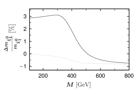
Figure 1: Comparison of relative corrections to $m_{\tilde{\chi}^{0}_{1}}$ [8]. The full line shows the case where the SUSY SU(5) GUT relation is assumed for the $\overline{\rm DR}$ parameters $M$ and $M^{\prime}$, and the on–shell $M^{\prime}$ is determined from $M$ by the same relation. The dotted line corresponds to the case where the on–shell $M^{\prime}$ is an independent parameter but satisfies the SUSY GUT relation. Other parameters are $\tan{\beta}=7$, $\{M_{\tilde{Q}_{1}},\,M_{\tilde{Q}},\,A\}=\{300,300,-500\}$ GeV, and $\mu=-220$ GeV.

Fig. 1 shows the correction to $m_{\tilde{\chi}^{0}_{1}}$ as a function of $M$ for $\tan{\beta}=7$, $\{M_{\tilde{Q}_{1}},\,M_{\tilde{Q}},\,A,\,\mu\}=\{300,300,-500,-110\}$ GeV. ($M_{\tilde{Q}_{1}}$ and $M_{\tilde{Q}}$ are soft breaking parameters of the first and third squark generation, respectively, and $A$ is the trilinear soft breaking parameter.) It can be seen that the difference between the case where the GUT relation is assumed also for the on–shell $M^{\prime}$ and $M$ and the case where $M^{\prime}$ is an independent parameter ($\Delta{Y}_{11}=0$) with the value $0.498$ (as it would have by the GUT relation) is substantial.

By the way, Eq. (45) would also be valid in the anomalously mediated SUSY breaking model [13, 14] where $M^{\prime}=11\tan^{2}\theta_{W}M$.

In conclusion, the method developed here is well suited for extracting and studying the fundamental SUSY parameters $M$, $M^{\prime}$, $\mu$, etc. at higher order.

3 Other on–shell methods of renormalizing
the chargino/neutralino system

A different method for the on–shell renormalization of the chargino and neutralino system was presented in [15]. The same method was also used in [16, 17, 18, 21].

Concerning the charginos, the input parameters are as before the physical chargino masses $m_{\tilde{\chi}^{+}_{1}}$ and $m_{\tilde{\chi}^{+}_{2}}$. The parameters $M$ and $\mu$ are calculated from the tree–level form of the mass matrix, Eq. (20), by diagonalization, Eq. (21).

The on–shell condition is that the renormalized two–point function matrix $\hat{\Gamma}^{(2)}_{ij}$ get diagonal for on–shell external momenta, i.e.

$${\rm Re}\,\hat{\Gamma}^{(2)}_{ij}(p)\,u_{j}(p)=0\,,$$ (46)

for $p^{2}=m_{\tilde{\chi}^{+}_{j}}^{2}$. This fixes the non-diagonal elements of the field-renormalization matrix. Its diagonal elements are determined by normalizing the residues of the propagators. These conditions then fix $\delta{M}$ and $\delta\mu$, but they are different from the expressions Eqs. (27).

In the neutralino sector, one has the additional parameter $M^{\prime}$ which is fixed together with its counter term $\delta{M^{\prime}}$ by a neutralino mass, say $m_{\tilde{\chi}^{0}_{1}}$, and the appropriate on–shell condition in analogy to Eq. (46). Hence one has

$$N\,Y\,N^{T}\,=\,{\rm diag}\left(m_{1},m_{2},m_{3},m_{4}\right)\,=\,M_{D}\,,\hskip 56.9055pt{\rm with}\;m_{1}=m_{\tilde{\chi}^{0}_{1}}\;\;{\rm(pole\;mass)}$$

$N$ is the mixing matrix in Eq. (37). $m_{2}$, $m_{3}$, $m_{4}$ are, however, not yet the one–loop corrected pole masses $m_{\tilde{\chi}^{0}_{i}}$, $i=2,3,4$. One has to find the momenta $p_{i}^{2}=m^{2}_{\tilde{\chi}_{i}^{0}}$ so that

$${\mathrm{R}e}\left[\hat{\Gamma}^{(2)}_{ii}(p_{i})\right]\,u(p_{i})\,=\,0\,,$$

with

$$\hat{\Gamma}^{(2)}_{ij}(p_{i})\,=\,\left({p/}-m_{i}\right)\delta_{ij}+\hat{\Sigma}_{ij}(p)\,,$$

where $\hat{\Gamma}^{(2)}$ is the renormalized two–point vertex function and $\hat{\Sigma}$ is the renormalized self–energy.

It should be clear from above that the parameters $M$, $M^{\prime}$, and $\mu$ derived by this method are different from those in section 2.2 and 2.3, and in [8], and of course also from those in the $\overline{\rm DR}$ scheme [9]. They are “effective” parameters. However, the observables (cross–section, branching ratios, particle masses, …) are the same in both methods.

4 One–loop corrections to SUSY processes

Let us start with a discussion of chargino production

$$e^{+}e^{-}\;\rightarrow\;{\tilde{\chi}^{+}_{i}}\,{\tilde{\chi}^{-}_{j}}\,.$$

Using the purely on–shell renormalization scheme described above in section 3, the full one–loop corrections to this process (including polarized beams) were calculated in [18]. This calculation is extremely cumbersome as one has to compute a large number of graphs (self–energy graphs, vertex corrections, box graphs) with all the particles of the MSSM running in the loops. A further subtlety is due to the contributions with virtual photons attached to two external charged particles. To obtain an infrared finite result, real photon bremsstrahlung from the external particles has to be taken into account. Without the virtual photons the result would not be UV finite. They are required to cancel the divergence coming from the photino component of the virtual neutralinos.

Figure 2: One–loop corrections to the cross–section of $e^{+}e^{-}\rightarrow\tilde{\chi}_{1}^{+}\tilde{\chi}_{1}^{-}$, normalized to the Born approximation [18]. Upper (lower) row: $M_{2}=200$ GeV (800 GeV), $\sqrt{s}=500$ GeV (1 TeV), $M_{\rm SUSY}=500$ GeV. The various lines show the contributions from different subsets of diagrams: the dash–dotted, long dashed, dashed and dotted line corresponds to (s)top/(s)bottom loops, (s)fermion loops, SM fermion loops and all loops without ISR.

Fig. 2 shows the relative one–loop correction $\Delta=\frac{\sigma-\sigma_{0}}{\sigma}$ ($\sigma_{0}$ being an improved Born cross–section) to the total cross–section of $e^{+}e^{-}\;\rightarrow\;{\tilde{\chi}^{+}_{1}}\,{\tilde{\chi}^{-}_{1}}$ as a function of $\tan\beta$ at $\sqrt{s}=500$ GeV and $\sqrt{s}=1$ TeV, with the parameters as indicated in the figure caption (The initial state radiation (ISR) is separated off). Typically, the corrections are between $5$ and $10$%, but can go up to more than 20% at $\sqrt{s}=1$ TeV. The figure also exhibits the contributions from various subsets of graphs. One clearly sees that the (s)top/(s)bottom loops are by far not enough to explain the full correction. The figure demonstrates the necessity of a complete full one–loop calculation.

A complete one–loop calculation for chargino production in $e^{+}e^{-}$ annihilation was also performed in [19]. However, the renormalization scheme is different. For the charginos as external particles the subtractions are made on–shell. The masses of all particles are also taken to be physical, but all other parameters (as couplings) are considered to be in the $\overline{\rm DR}$ scheme at the scale $m_{Z}$. In [19] the one–loop corrections to the chargino production helicity amplitudes (with polarized beams) are calculated. However, pure QED corrections involving loops of photons were omitted.

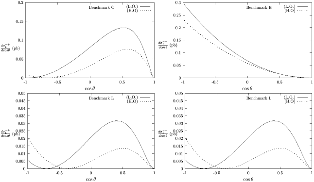
Figure 3: Lowest and higher order cross–section $\sigma_{L}^{-+}$ for $e^{+}e^{-}\rightarrow\tilde{\chi}_{1}^{+}\tilde{\chi}_{1}^{-}$ with left–polarized electrons and negative (positive) helicity of the chargino $\tilde{\chi}_{1}^{+}$ ($\tilde{\chi}_{1}^{-}$) [19].

In Fig. 3 $\frac{d\sigma^{-+}_{L}}{d{\cos{\theta}}}$ is shown as a function of $\cos{\theta}$ for various benchmark scenarios [20]. $\sigma^{-+}_{L}$ is the cross–section for producing a negative helicity chargino and a positive helicity anti-chargino with a left–handed electron. Shown are the tree–level cross–sections and the one–loop corrected ones. The corrections can be very large ($>50\%$), especially if the cross–section is low.

The other processes for which full one–loop corrections were calculated [21] are

$$e^{+}e^{-} \rightarrow \tilde{\mu}_{R}^{+}\tilde{\mu}_{R}^{-}\,\;,\tilde{\mu}_{L}^{+}\tilde{\mu}_{L}^{-}\,,$$

$$e^{\pm}{e}^{-} \rightarrow \tilde{e}^{\pm}_{R}\tilde{e}^{-}_{R}\,\;,\tilde{e}^{\pm}_{L}\tilde{e}^{-}_{L}\,\;,\tilde{e}^{\pm}_{R}\tilde{e}^{-}_{L}\,\;,\tilde{e}^{\pm}_{L}\tilde{e}^{-}_{R}\,\;,$$ (47)

with polarized $e^{+}$ and $e^{-}$ beams.

Especially for $e^{+}e^{-}\rightarrow\tilde{e}^{+}\tilde{e}^{-}$ the calculation is rather complex because of the neutralino exchanges in the t-channel. One has to renormalize the neutralino sector.

Figure 4: Electroweak corrections to the cross–section of (a) $e^{+}e^{-}\rightarrow\tilde{e}_{R}^{+}\tilde{e}_{R}^{-}$, (b) $e^{-}e^{-}\rightarrow\tilde{e}_{R}^{-}\tilde{e}_{R}^{-}$, relative to the Born cross–section [21]. Input parameters correspond to the SPS1 scenario.

Fig. 4a shows the $\sqrt{s}$ dependence of the full electroweak corrections ${(\sigma-\sigma_{\rm Born})}/{\sigma_{\rm Born}}$ for $e^{+}e^{-}\rightarrow\tilde{e}_{R}^{+}\tilde{e}_{R}^{-}$. The input values correspond to the SP1 scenario [22], with the mSUGRA point $m_{0}=100$ GeV, $M_{1/2}=250$ GeV, $A_{0}=-100$ GeV, $\tan\beta=10$, $\mu>0$. The “universal” initial state radiation (ISR) has been subtracted. However, the process dependent QED corrections are included. For illustration, also the contributions from various subsets of diagrams are shown. One can see that the (s)lepton loops and (s)quark loops do not account for the whole effect. This means that the gauge boson, Higgs boson, gaugino and higgsino exchanges are important. In total, the corrections are $\leq|10|\%$. Fig. 4b shows the corresponding electroweak correction as a function of $\sqrt{s}$ for
$e^{-}e^{-}\rightarrow\tilde{e}_{R}^{-}\tilde{e}_{R}^{-}$.

Figure 5: Dependence of the relative one–loop corrections $\Delta_{\alpha}$ on the universal squark soft breaking parameter $M_{\tilde{Q}}$ to the cross–section of (a) $e^{+}e^{-}\rightarrow\tilde{\mu}^{+}_{R}\tilde{\mu}^{-}_{R}$ for $\sqrt{s}=500$ GeV, and (b) to $e^{-}e^{-}\rightarrow\tilde{e}^{-}_{R}\tilde{e}^{-}_{R}$ for $\sqrt{s}=400$ GeV [21]. Input parameters correspond to the SPS1 scenario.

In Fig. 5 the dependence of the one–loop corrections is exhibited as a function of the soft breaking parameter $M_{\tilde{Q}}=m_{\tilde{q}_{L}}=m_{\tilde{u}_{R}}=m_{\tilde{d}_{R}}$. (The other parameters are as in the SPS1 scenario.) Fig. 5a shows the behaviour for $\tilde{\mu}_{R}^{+}\tilde{\mu}_{R}^{-}$ production at $\sqrt{s}=500$ GeV. One sees that for large $M_{\tilde{Q}}$ the correction reach an asymptotic value being an indication for the decoupling of the squarks. In contrast, Fig. 5b shows the corresponding $M_{\tilde{Q}}$-dependence for $\tilde{e}_{R}^{-}\tilde{e}_{R}^{-}$ production at $\sqrt{s}=400$ GeV. In this case, the size of the radiative corrections increases with $M_{\tilde{Q}}$ showing no decoupling. This is due to the so–called superoblique corrections [23]. These stem from squark–quark loops in neutralino self–energies.

For the squark pair production process

$$e^{+}e^{-}\rightarrow\;\;\tilde{q}_{i}\;\bar{\tilde{q}}_{j}\,,\hskip 56.9055pt{\rm with}\;\;j=1,2\;;\;\;\tilde{q}=\tilde{t},\tilde{b}$$

only the SUSY–QCD corrections [24] and the Yukawa corrections due to quark and squark loops have been calculated [6]. Whereas the QCD corrections are typically 15–20%, the Yukawa corrections are $<|10\%|$ of the tree–level cross–section.

Very recently, the next–to–leading SUSY–QCD corrections have been calculated [25] for

$$e^{+}e^{-}\rightarrow\;\;q\;\bar{q}\;g$$

$$e^{+}e^{-}\rightarrow\;\;\tilde{q}\;\bar{\tilde{q}}\;g$$

$$e^{+}e^{-}\rightarrow\;\;q\;\bar{\tilde{q}}\;\tilde{g}$$

where $q$ denotes a light quark, and the squarks have no mixing. By comparing these reactions the equality of the $q\,q\,g$, the $\tilde{q}\,\tilde{q}\,g$, and the Yukawa coupling $q\,\tilde{q}\,\tilde{g}$ in the supersymmetric limit ($m_{\tilde{q}}=m_{q}$, $m_{\tilde{g}}=m_{g}=0$) can be tested.

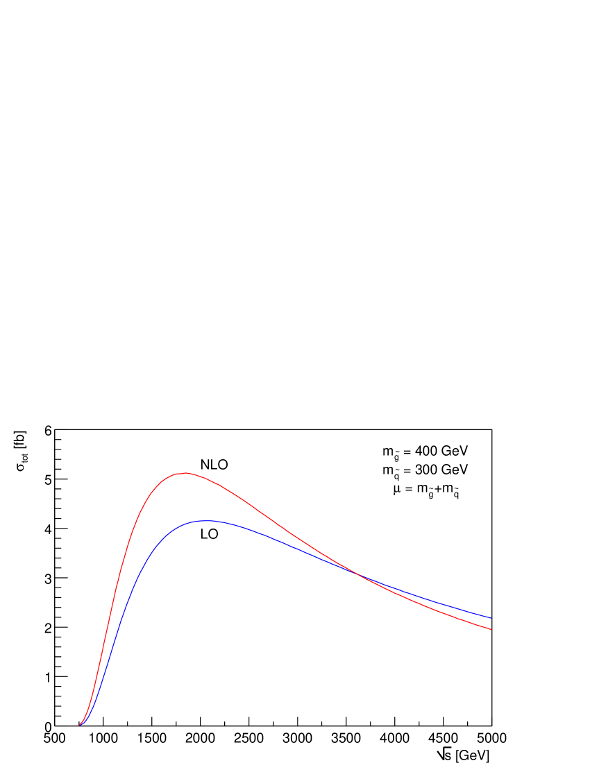
Figure 6: Total cross–section for $e^{+}e^{-}\rightarrow\tilde{q}\,\bar{q}\,\tilde{g}\,(g)+q\ \bar{\!\tilde{q}}\,\tilde{g}\,(g)$ in leading (LO) and next–to–leading (NLO) order, as a function of $\sqrt{s}$ [25].

Fig. 6 shows as a function of $\sqrt{s}$ the cross–section in leading order (LO) and next–to–leading order(NLO) for $e^{+}e^{-}\rightarrow\,\;\tilde{q}\,\bar{q}\,\tilde{g}\,(g)\,+\,q\ \bar{\!\tilde{q}}\,\tilde{g}\,(g)$, summed over $u$, $d$, $c$, $s$, $b$ quarks; $m_{{\tilde{g}}}=400$ GeV, $m_{\tilde{q}}=300$ GeV and $\mu=m_{\tilde{g}}+m_{\tilde{q}}$. The cross–section goes up to 5 fb. At the peak the corrections are about  20%, enhancing the LO cross–section.

4.1 Decays of supersymmetric particles

The SUSY–QCD corrections to the decays

$${\tilde{q}}_{i} \rightarrow q\,{\tilde{\chi}^{0}_{i}}\;,\hskip 85.35826pti=1,..,4$$

$${\tilde{q}}_{i} \rightarrow q\,{\tilde{\chi}^{\pm}_{k}},\hskip 85.35826ptk=1,2$$

were already calculated some time ago [26]. The full electroweak corrections were computed recently in [16].

Figure 7: Relative electroweak radiative corrections to the partial widths of the lightest stop decaying into charginos and neutralinos [16]. $\delta_{+}^{11}$ corresponds to $\tilde{t}_{1}\rightarrow b\,\tilde{\chi}_{1}^{+}$, $\delta_{+}^{12}$ to $\tilde{t}_{1}\rightarrow b\,\tilde{\chi}_{2}^{+}$, $\delta_{0}^{11}$ to $\tilde{t}_{1}\rightarrow t\,\tilde{\chi}_{1}^{0}$, $\delta_{0}^{12}$ to $\tilde{t}_{1}\rightarrow t\,\tilde{\chi}_{2}^{0}$ and $\delta_{0}^{13}$ to $\tilde{t}_{1}\rightarrow t\,\tilde{\chi}_{3}^{0}$.

Fig. 7 shows the $m_{{\tilde{t}}_{1}}$ dependence of the relative electroweak corrections $\delta$ to the partial widths of ${\tilde{t}}_{1}\rightarrow{b}\,{\tilde{\chi}^{+}_{1}},\,{b}\,{\tilde{\chi}^{+}_{2}}$, ${\tilde{t}}_{1}\rightarrow{t}\,{\tilde{\chi}^{+}_{1}},\,{t}\,{\tilde{\chi}^{0}_{2}},\,{t}\,{\tilde{\chi}^{0}_{3}}$ for the parameter set
$\{M,\,\mu,\,\tan\beta,\,\theta_{\tilde{t}},\,m_{{\tilde{b}}_{1}},\,\theta_{\tilde{b}},\,M_{H^{+}}\}=\{150\,{\rm GeV},-100\,{\rm GeV},\,4,\,0.6,\,300\,{\rm GeV},\,0.3,\,120\,{\rm GeV}\}$. They go up to 20%. The various spikes are due to the opening of other decay channels. Although the QCD corrections are usually dominant, the electroweak corrections can be of the same size in certain regions of the parameter space.

The decays of a squark into a quark and gluino, and of a gluino into a squark and quark

$${\tilde{q}}_{i} \rightarrow q\,{\tilde{g}}$$

$${\tilde{g}} \rightarrow {\tilde{q}}_{i}\,q\hskip 85.35826pti=1,2$$

were calculated including one–loop SUSY–QCD corrections in [27]. The corrections can go up to 50%.

The Yukawa corrections up to ${\cal O}(\alpha_{ew}m_{q}^{2}/m_{W})$ to ${\tilde{t}}_{2}\rightarrow t\,{\tilde{g}}$ and ${\tilde{g}}\rightarrow\bar{t}\,{\tilde{t}}_{1}\;+c.c.$ were calculated in [28]. They reach values of $\sim 10\%$.

The SUSY–QCD corrections to the decays

$${\tilde{t}}_{i}\rightarrow{\tilde{b}}_{j}W^{+}\,,\;\;\;{\tilde{b}}_{i}\rightarrow{\tilde{t}}_{j}W^{-}\hskip 28.45274pt{\rm\;and\;}\hskip 28.45274pt{\tilde{t}}_{2}\rightarrow{\tilde{t}}_{1}Z^{0}\,,\;\;\;{\tilde{b}}_{2}\rightarrow{\tilde{b}}_{1}Z^{0}$$ (48)

were computed in [29]. The squark decays into Higgs bosons

$${\tilde{q}}_{i} \rightarrow {\tilde{q}}_{j}^{(\prime)}\,H_{m}\hskip 85.35826ptH_{m}=\{h^{0},\,H^{0},\,A^{0},\,H^{\pm}\}\,.$$ (49)

including SUSY–QCD corrections have been treated in [30, 31]. For the Higgs boson decays into squarks

$$H_{m} \rightarrow {\tilde{q}}_{i}\,\bar{\tilde{q}}^{(\prime)}\,,$$

these corrections were calculated in [30, 32]. In the on–shell scheme, they can become very large for large $\tan\beta$ (as in the case of $H_{l}\rightarrow{q}\bar{q}$), making the perturbation expansion quite unreliable. An improvement of the perturbation calculation was proposed in [33]. This is achieved by using the SUSY–QCD running quark mass $m_{q}(Q)_{\rm MSSM}$ and the running trilinear coupling $A_{q}(Q)$ in the tree–level coupling. However, the mixing angle $\theta_{\tilde{q}}$ is kept on–shell in order to cancel the ${\tilde{q}}_{1}-{\tilde{q}}_{2}$ mixing squark wave–function correction.

The one–loop corrected decay widths for

$$H_{m} \rightarrow {\tilde{\chi}^{0}_{k}}\,{\tilde{\chi}^{0}_{l}}$$

$${\tilde{\chi}^{0}_{k}} \rightarrow H_{m}\,{\tilde{\chi}^{0}_{l}}$$ (50)

were calculated in [34] taking into account all fermion and sfermion loop contributions. The neutralino mass matrix was renormalized as described in section 2.4.

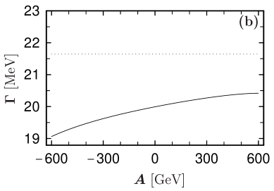
Figure 8: The widths of the decays $H^{0}\to{\tilde{\chi}}^{0}_{1}+{\tilde{\chi}}^{0}_{2}$ (a) and $A^{0}\to{\tilde{\chi}}^{0}_{1}+{\tilde{\chi}}^{0}_{3}$ (b) as a function of $A$ [34]. The dotted line corresponds to the tree–level width, the solid line corresponds to the full correction. The parameters are $\tan{\beta}=10$, $M=500$ GeV, and $\mu=150$ GeV (a) and $\tan{\beta}=50$ and $M=\mu=300$ GeV (b).

Fig. 8 shows the correction to the width of $H^{0}\rightarrow{\tilde{\chi}^{0}_{1}}{\tilde{\chi}^{0}_{2}}$ and $A^{0}\rightarrow{\tilde{\chi}^{0}_{1}}{\tilde{\chi}^{0}_{3}}$ as a function of the trilinear coupling $A$ for the parameters as given in the figure caption.

The decays into charginos

$$H^{0}(A^{0}) \rightarrow {\tilde{\chi}^{+}_{i}}{\tilde{\chi}^{-}_{j}}$$

$$H^{+} \rightarrow {\tilde{\chi}^{+}_{i}}{\tilde{\chi}^{0}_{l}}$$

were treated in the same approximation in [35].

5 Conclusions

Precision experiments which will be possible at a future linear $e^{+}e^{-}$ collider will require equally precise theoretical calculations of cross–sections, decay branching ratios and other observables, including higher order corrections. For doing such calculations, we have presented the on–shell renormalization of the sfermion and chargino/neutralino system in the MSSM. We have worked out the appropriate renormalization conditions, especially for the mixing matrices. We have discussed the calculations of one–loop corrections to various SUSY processes: sfermion and chargino/neutralino production in $e^{+}e^{-}$–annihilation, the two–body decays of sfermions and the decays of Higgs bosons into SUSY particles. In a few cases the full electroweak corrections have already been calculated. They clearly show that taking only a subset of diagrams, for instance, only (s)top/(s)bottom loops, is not sufficient. The electroweak corrections are typically between 5 and 15%, but can go up to larger values for certain parameters. Although the QCD corrections are usually the largest ones, the electroweak corrections can be of the same size in certain cases.

References

- [1] TESLA Technical Design Report, Part III, Physics at an Linear Collider, Eds.: R. D. Heuer, D. Miller, F. Richard, and P. M. Zerwas, DESY 2001-011, (2001).
- [2] W. Hollik et al., Nucl. Phys. B 639 (2002) 3.
- [3] W. Siegel, Phys. Lett. B 84 (1979) 193; D. M. Capper, D. R. T. Jones, P. von Nieuwenhuizen, Nucl. Phys. B 167 (1980) 479.
- [4] K. Fujikawa, B. W. Lee, A. I. Sanda, Phys. Rev. D 6 (1972) 2923 ; E. S. Abers and B. W. Lee, Phys. Rep. 9 (1973) 1.
- [5] J. Guasch, J. Sola, W. Hollik, Phys. Lett. B 437 (1998) 88.
- [6] H. Eberl, S. Kraml, W. Majerotto, JHEP 9905 (1999) 016.
- [7] Y. Yamada, talk at this conference, hep-ph/0103046.
- [8] H. Eberl, M. Kincel, W. Majerotto, and Y. Yamada, Phys. Rev. D 64 (2001) 115013.
- [9] D. Pierce et al., Nucl. Phys. B 491 (1997) 3.
- [10] P. H. Chankowski, S. Pokorski, J. Rosiek, Nucl. Phys. B 423 (1994) 437.
- [11] A. Dabelstein, Z. Phys. C 67 (1995) 495.
- [12] Y. Yamada, hep-ph/9608382; hep-ph/0112251; A. Freitas, D. Stöckinger, hep-ph/0205281.
- [13] L. Randall and R. Sundrum, Nucl. Phys. B 557 (1999) 79; G. F. Giudice, M. Luty, H. Murayama, and R. Rattazzi, JHEP 9812 (1998) 027.
- [14] J. L. Feng, T. Moroi, L. Randall, M. Strassler, and S. Su, Phys. Rev. Lett. 83 (1999) 1731.
- [15] T. Fritzsche and W. Hollik, hep-ph/0203159.
- [16] J. Guasch, W. Hollik, and J. Sol Phys. Lett. B 510 (2001) 211; J. Guasch, W. Hollik, J. Sola, hep-ph/0207364.
- [17] T. Blank and W. Hollik, hep-ph/0011092.
-
[18]
T. Blank, Dissertation (in German), TH Karlsruhe (2000),
http://www-itp.physik.uni-karlsruhe.de/prep/phd/PSFiles/phd-1-2000.ps.gz;
T. Blank and W. Hollik, hep-ph/0011092. - [19] M. A. Diaz and D. Ross, hep-ph/0205257.
- [20] M. Battaglia et al., hep-ph/0112013.
- [21] A. Freitas, Dissertation, Hamburg (2002), talk at the Workshop of the ECFA/DESY Study on a Linear Collider, St. Malo, France, April 2002.
- [22] N. Ghodbane and H. V. Martyn, in Proc. of the APS/DPF/DPB Summer Study on the Future of Particle Physics (Snowmass 2001), ed. R. Davidson and C. Quigg; hep-ph/0201233.
- [23] M. M. Nojiri, K. Fujii, T. Tsukamoto, Phys. Rev. D 54 (1996) 6756; H. C. Cheng, J. L. Feng, and N. Polonsky, Phys. Rev. D 56, (1997) 6875; hep-ph/9706438.
- [24] A. Arhrib, M. Capdequi Peyranre, A. Djouadi, Phys. Rev. D 52 (1995) 1404; H. Eberl, A. Bartl, W. Majerotto, Nucl. Phys B 472 (1996) 481.
- [25] A. Brandenburg, M. Maniatis, M. M. Weber, talk at this conference, hep-ph/0207278.
- [26] S. Kraml et al., Phys. Lett. B 386 (1996) 175; A. Djouadi, W. Hollik, C. Jünger, Phys. Rev. D 55 (1997) 6975.
- [27] W. Beenaker, R. Höpker, and P. M. Zerwas, Phys. Lett. B 378 (1996) 159; W. Beenaker et al., Z. Phys. C 75 (1997) 349.
- [28] Hou Hong-Shang et al., hep-ph/0202032.
- [29] A. Bartl et al., Phys. Lett. B 419 (1998) 243.
- [30] A. Arhrib et al., Phys. Rev. D 57 (1998) 5860.
- [31] A. Bartl et al.: Phys. Rev. D 59 (1999) 115007.
- [32] A. Bartl et al.,Phys. Lett. B 402 (1997) 303.
- [33] H. Eberl et al., Phys. Rev. D 62 (2000) 055006.
- [34] H. Eberl et al., Nucl. Phys. B 625 (2002) 372.
- [35] Zhang Ren-You et al., hep-ph/0201132.