hep-ph/0209135

DO-TH 02/15

In the framework of NRQCD and parton model, we estimate in detail, the production cross section for polarized $J/\psi$ from $B$ meson decays. In order to contrast with data, we also take into account additional $J/\psi$ production due to decay of excited charmonium states. We calculate the helicity parameter, $\alpha$, and as an application, we study our results for the Tevatron. This is in contrast to the earlier studies which were performed for prompt $J/\psi$ production from $p\bar{p}$ collisions. Our estimates are, for $J/\psi$ from $B$ decays, $\alpha_{J/\psi}=-0.04\pm 0.06$ and for $B$ decays to $\psi^{\prime}$, $\alpha_{\psi^{\prime}}=-0.03\pm 0.07$. These results have been evaluated in the $J/\psi$ transverse momentum interval, $10~{}\mbox{GeV}\leq k_{T}\leq 30~{}\mbox{GeV}$. In the limit of the color singlet model, $\alpha$ shows a direct dependence on the Peterson parameter, thereby reflecting the dynamics of the $b$ quark hadronization. With Run II of the Tevatron, it is expected that the fits for $\alpha$ will improve by about a factor of 50, leading to better limits on the matrix elements.

1 Introduction

The production mechanism of bound states involving a heavy quark and anti-quark system can be addressed within non-relativistic quantum chromodynamics (NRQCD) [1]. In the earliest attempts, charmonium production was described by the color singlet model through processes like $B$ decays $(b\rightarrow c\bar{c}s)$ [2, Wise:1980tp, Kuhn:1980zb] and gluon-gluon fusion $(gg\rightarrow c\bar{c}g)$ [Chang:1980nn]. We refer to [Schuler:1994hy] for a review on these issues. However, the color singlet models had several problems, e.g., underestimation of the hadroproduction of charmonium [Vanttinen:1995sd], the $\psi^{\prime}$ anomaly [Braaten:1994xb, Roy:1994ie] and infrared divergences in $P$ wave charmonium production, which later had a resolution based on factorization results [Bodwin:1995jh, Bodwin:1992ye]. These problems suggested the need to advance beyond the color singlet model or similar variants like the color evaporation model [Fritzsch:1977ay]. In a systematic approach, by including the color octet contributions within the NRQCD framework it was shown that these problems could indeed be resolved to a good accuracy [Beneke:1996yb, Beneke:1996tk, Beneke:1996xg].

Within NRQCD, which is well designed for separating relativistic from non-relativistic scales, Bodwin, Braaten and Lepage developed a factorization formalism to calculate quarkonium decays and production [Bodwin:1995jh]. The formalism allows for a systematic calculation of the inclusive cross sections to any order in strong coupling $\alpha_{s}$, and an expansion in $v^{2}$. Here, $v$ is the relative velocity of the quark and antiquark and is inversely proportional to the heavy quark mass. As an illustration, following potential model calculations, for bottonium states, ${v\sim 0.1}$ while for charmonium states, ${v\sim 0.3}$ indicating a better convergence in the perturbative expansion for heavier quark states [Quigg:1979vr]. It is interesting to observe that the theory exhibits a scale hierarchy of the type, ${m_{Q}\gg m_{Q}v\gg m_{Q}v^{2}\sim\Lambda_{\textrm{QCD}}}$, where $m_{Q}$ is the heavy quark mass. Therefore, it is appropriate to use NRQCD as an effective field theory with $v$ as the expansion parameter which is also a naturally small scale of the theory. In addition, at leading order in $v$, NRQCD has a strong correspondence to a $1/m_{Q}$ expansion as in heavy quark effective theory.

A large fraction of the existing literature on NRQCD employing the factorization formalism, broadly concentrates on one of the following two issues; (i) on prompt charmonium production in hadron [Leibovich:1997pa, Braaten:1999qk, Tang:1996zp, Beneke:1996yb], $\gamma p$ and $ep$ [Fleming:1997jx] and in $e^{+}e^{-}$ [Chang:1997dw, Yuan:1997sn, Boyd:1998km, Klasen:2001cu] collisions or (ii) on charmonium production in hadronic $B$ decays [Bodwin:1992qr, Kniehl:1999vf, Beneke:1999gq]. Prompt production refers to quarkonium (here charmonium) that is created in interactions of the colliding particles or their constituents, while charmonium production is also possible in weak decays of $B$ mesons, which will be the focus of the present work. At the functional level, the calculations in case (i) have been adopted to phenomenologically extract NRQCD matrix elements from experimental data on charmonium production. This is possible, because these calculations incorporate bound state effects of the initial hadronic states, usually in the framework of the QCD improved parton model (PM). In the case of semi-inclusive $B$ decays with charmonium final states, the ACCMM model [Altarelli:1982kh] and the PM [Palmer:1997wv] have been successfully adopted for this description. A central feature of these results has been to illustrate the importance of color octet elements to accommodate the observed momentum spectra of $J/\psi$.

Quarkonium polarization provides an additional test of the color octet production mechanism of NRQCD [Beneke:1997jh]. The polarized cross section has been calculated for prompt $\psi$ production [Leibovich:1997pa] as well as for $J/\psi$ production in $b$ quark decays [Fleming:1997pt]. We remark that, in the case of $J/\psi$ production from $b$ decays, the calculations do not take into account bound state effects, although they have been estimated to be significant [Ma:2000bz]. Hence, a comparison with data in this case may not be too meaningful, given the uncertainties, originating from the negligence of the initial hadron, and the additional errors due to the non-perturbative NRQCD matrix elements. As a salient prediction, within NRQCD, prompt charmonium production is expected to be predominantly in transverse polarization state for large transverse momenta $(p_{T})$ [Beneke:1996yb, Leibovich:1997pa, Braaten:1999qk, Cho:1995ih]; but this prediction is not in agreement with the CDF data [Affolder:2000nn]. We note that the polarization prediction arises from the dynamics of massless partons and for large $p_{T}$, the role of gluon dynamics is important in prompt quarkonium production, especially through the dominance of gluon fragmentation [Braaten:1993rw]. Furthermore, a gluon couples easily to the ${}^{3}S_{1}$ color octet state, which is expected to be a dominant spectral state in the prompt $J/\psi$ production mechanism at the Tevatron. But correspondingly, the charmonium production at large transverse momenta (with $p_{T}\geq 20$ GeV) are not fully probed by current experiments. Besides, there are large errors in the polarization measurements. Therefore, these features alone preclude any possible conclusions on the predictions by NRQCD for polarized charmonium production.

On the other hand, at moderate transverse momenta (with $p_{T}\leq 20$ GeV), one can perform the polarization studies for prompt charmonium production to make an estimate of the color octet elements and also compare with the unpolarized cross sections. This is of particular relevance to the Tevatron where there are no complications due to higher twist effects [Beneke:1997yw]. We refer to [Lee:2002au] for an update on prompt production of polarized charmonium for the Tevatron. Simultaneously, one can also study the charmonium production which is not prompt and in particular estimate the cross sections for polarized production.

It is the goal of the present work to analyze the polarization predictions for $J/\psi$ from $B$ meson decays at the Tevatron. Unlike in the case of prompt production, in this process, we do not expect gluon fragmentation as a dominant source for $J/\psi$ production, which led to predominantly transverse polarized $J/\psi$. Therefore, our calculation can serve as an independent probe of NRQCD dynamics for polarized charmonium production, besides the existing knowledge from prompt production. We employ the PM approach as discussed in [Palmer:1997wv] to fold the quark level calculations to arrive at a $B$ hadron decay. We calculate the helicity parameter, $\alpha$, from the production cross section of the three polarization states of the $J/\psi$. We observe that a significant drawback of any such analysis are due to our present poor understanding of the relevant NRQCD matrix elements. As an outcome of our approach, we note that in the color singlet model (when the octet elements are set to zero), the $\alpha$ prediction reduces to the details of bound state effects of the PM. In other words, $\alpha$ depicts a strong dependence on the Peterson fragmentation function which describes the Fermi motion of the $b$ quark in the $B$ meson. In some sense, this result is also to be anticipated simply on grounds that the color singlet model predictions depend on the shape and form of the initial state wave function of the decaying system. With data from Run II of Tevatron, which is expected to increase the accuracy by a factor of 50, our analysis may be useful to tighten the estimates for the matrix elements significantly and make our polarization estimates more precise [Anikeev:2001rk]. In addition, in the future, a complete global fit/analysis to quarkonium production will certainly make the predictions more robust.

Our paper is organized as follows. In the next section, for completeness, we review the basic ideas of NRQCD pertinent to our calculations. In section 3, we introduce the effective Hamiltonian which describes the quarkonium production process through free $b$ quark decays. Using this formalism, we study the semi-inclusive decay of a free $b$ quark into $J/\psi$. The short-distance coefficients and the NRQCD matrix elements are explicitly calculated and the decay width is presented for $b\to J/\psi(\lambda)+X$. Here, $\lambda$ denotes one of the three helicity states of $J/\psi$. Towards the end of this section, we also discuss an extension of our calculations to excited charmonium states. The bound state effects of the initial $B$ meson, whose influence hitherto has been neglected in the calculation, are described in section 4. In this analysis, we use the PM approach to evaluate the bound state effects. Starting with a short introduction to the PM, the restrictions of the model applicability and estimates for the semi-inclusive decay rate for a $B$ meson with a charmonium final state are presented. This is followed by section 5, where we describe the application of the results derived so far to the Tevatron and introduce suitable kinematic variables. In section 5.1, we discuss the production cross section for polarized $J/\psi$ at the Tevatron. In order to phenomenologically implement the production cross section for $B$ mesons at the Tevatron, we introduce a simple two-parameter fit procedure. In section 6, we describe the relevant NRQCD matrix elements which we use for this analysis and also discuss the various sources of input errors for our estimates. Following this, in section 7, we give our detailed numerical estimates for the polarized cross section and predictions for the helicity parameter, $\alpha$. We also discuss the relevance/influence of the various theoretical input errors to our predictions. The differential cross section for $J/\psi$ and $\psi^{\prime}$ production from $B$ decays and the corresponding polarization parameter $\alpha$ are displayed and compared with current experimental data [Affolder:2000nn]. Since, the data includes feed-down channels from excited charmonium states, we account for this in our analysis to derive the polarization cross sections. Finally in section 8, we conclude with a summary of the results and comment on further possible improvements to the precision of our calculation. In the appendix of this paper, we have tabulated all the relevant matrix elements and their sources and give the values which we use in our analysis.

2 Basic formalism

In [Bodwin:1995jh], it was shown that effects of the lower momentum scales of the order, $m_{Q}\cdot v$, $m_{Q}\cdot v^{2}$ and $\Lambda_{\textrm{QCD}}$ can be factored into matrix elements that are accessible only via non-perturbative techniques or from experiments. On the other hand, the short distance contributions that occur on scales larger than the heavy quark mass, can be calculated within perturbative QCD. A matching prescription is required to identify the perturbatively calculated short-distance part and the non-perturbative NRQCD matrix elements. In the following, we recollect this matching procedure for polarized quarkonium production which we shall later use for our calculation. This is followed by a basic description of the matrix elements and their scaling properties.

2.1 The matching procedure

Let us consider an inclusive production of a quarkonium state $H$ with momentum $k$ and helicity $\lambda$ via a parton level decay process of the type $I\to H(k,\lambda)+X$. The semi-inclusive decay width is given as

$$\sum\limits_{X}d\Gamma(I\to H(k,\lambda)+X)=\frac{1}{2E}\frac{d^{3}k}{(2\pi)^{3}2E_{H}}\sum\limits_{X}(2\pi)^{4}\delta^{(4)}(p-k-p_{X})|{\cal T}_{I\to H(k,\lambda)+X}|^{2}~{},$$ (1)

where $E$ and $\boldsymbol{p}$ are energy and momentum of the decaying particle, $E_{H}$ is the energy of the quarkonium and the sum over $X$ includes the phase space integration for the additionally produced particles. On the other hand, from the NRQCD factorization theorem, the decay width in (1) can be factorized into short-distance coefficients and long-distance matrix elements of local four-quark operators. Formally,

$$\sum\limits_{X}d\Gamma(I\to H(k,\lambda)+X)=\frac{1}{2E}\frac{d^{3}k}{(2\pi)^{3}2E_{H}}\sum\limits_{m,n}C_{mn}(p,k)\times\langle{\cal O}_{mn}^{H(\lambda)}\rangle~{}.$$ (2)

In (2), the short-distance coefficients $C_{mn}$ ($m$ and $n$ denote some quantum numbers of the various states) depend only on kinematical quantities such as momenta and masses of the involved particles. They include effects of distances of the order $1/m_{Q}$ and smaller, where $m_{Q}$ is the mass of the quarks from which the quarkonium $H$ is built. The matrix elements, $\langle{\cal O}_{mn}^{H(\lambda)}\rangle$, are expectation values of local four-quark operators, sandwiched between vacuum states, $\langle 0|\ldots|0\rangle$ . These cannot be calculated perturbatively, but are extracted from experiment or from lattice calculations.

As a passing remark, we note that if the decaying particle is a hadron, then the parton level decay width in (2) must be folded with a suitable distribution function for the parton in the initial hadronic state. In this case, the factorization approximation requires the final quarkonium state to carry a large relative transverse momentum compared to $\Lambda_{\textrm{QCD}}$ [Bodwin:1995jh, Braaten:1996jt].

The typical four-quark operators which are related to the long-distance matrix elements have the general structure

$${\cal O}_{mn}^{H(\lambda)}=\psi^{\dagger}{\cal K^{\prime}}_{m}^{\dagger}\chi{\cal P}_{H(\lambda)}\chi^{\dagger}{\cal K}_{n}\psi~{},$$ (3)

where $\psi$ and $\chi$ are the heavy quark and antiquark non-relativistic field operators, respectively, and ${\cal K}_{n}$ and ${\cal K^{\prime}}_{m}^{\dagger}$ are products of spin and color matrices as well as covariant derivatives. Here, ${\cal P}_{H(\lambda)}$ is a projection operator that projects onto the subspace of states that contains the quarkonium state $H(\lambda)$ and in addition soft hadronic final states denoted by $S_{X}$. These soft states are supposed to be light, due to the NRQCD cut-off requirement, i.e. their total energy has to be less than the NRQCD ultraviolet cut-off $\Lambda$ to avoid double counting. Hence including them, ${\cal P}_{H(\lambda)}$ is written as

$${\cal P}_{H(\lambda)}=\sum\limits_{S_{X}}|H(\boldsymbol{k}=0,\lambda)+S_{X}\rangle\langle H(\boldsymbol{k}=0,\lambda)+S_{X}|~{}.$$ (4)

The matching procedure between the complete theory and the NRQCD expression requires that the normalization of the mesonic states in both the frameworks, i.e., in (1) and (2) be the same. In this analysis, we follow the relativistic normalization procedure as suggested in [Braaten:1996jt]. The matching condition is given as

$$\sum\limits_{X}(2\pi)^{4}\delta^{(4)}(p-k-p_{X}){\cal T}^{\ast}_{I\to c\bar{c}^{\prime}+X}{\cal T}_{I\to c\bar{c}+X}=\sum\limits_{m,n}C_{mn}(p,k)\langle\psi^{\dagger}{\cal K^{\prime}}_{m}^{\dagger}\chi{\cal P}_{H(\lambda)}\chi^{\dagger}{\cal K}_{n}\psi\rangle~{}.$$ (5)

To carry out the matching procedure explicitly, both the l.h.s. and the r.h.s. of (5) have to be expanded as a Taylor series in $\boldsymbol{q}$ and $\boldsymbol{q}^{\prime}$. The short-distance coefficients can then be simply identified by an order by order comparison in the coupling constant along with $\boldsymbol{q}$ and $\boldsymbol{q}^{\prime}$.

2.2 Expansion and simplification of matrix elements

As mentioned above, an expansion of the matrix elements is necessary for matching with the complete theory. In addition, by applying the symmetries of NRQCD the matrix elements are simplified and expressed in terms of standard matrix elements. The relative magnitudes of each of the matrix elements can be estimated, using velocity-scaling rules which we list here.

In the case of $J/\psi$, the independent matrix elements can be determined by simple tensor analysis, since it is a vector meson with $J=1$. Therefore, the helicity label, $\lambda$, transforms like a vector index in a spherical basis. This corresponds to choosing circular polarization vectors as the basis vectors for the polarization states of $J/\psi$. A unitary transformation, given by the matrix

$$\epsilon_{i}^{\lambda}=\left(\begin{array}[]{ccc}-1/\sqrt{2}&-i/\sqrt{2}&0\\ 0&0&1\\ 1/\sqrt{2}&-i/\sqrt{2}&0\end{array}\right)~{},$$ (6)

connects the two basis. Here, $i$ runs from $1$ to $3$, whereas $\lambda$ takes the values $+1$, $0$ and $-1$. In what follows, we list the matrix elements that appear in the calculation of $\psi$ production in $b$ quark decays. Rotational symmetry as well as heavy quark spin symmetry allow them to be expressed in terms of standard matrix elements [Bodwin:1995jh] with well defined spectral states, ${}^{2S+1}L_{J}$. Details on the expansion and reduction of NRQCD matrix elements can be found in [Braaten:1996jt]. For the simplest matrix elements without any vector indices one finds

$$\langle\psi^{\dagger}\chi{\cal P}_{J/\psi(\lambda)}\chi^{\dagger}\psi\rangle =\tfrac{4}{3}m_{c}\langle{\cal O}_{1}^{J/\psi}(^{1}S_{0})\rangle~{},$$ (7)

$$\langle\psi^{\dagger}T^{a}\chi{\cal P}_{J/\psi(\lambda)}\chi^{\dagger}T^{a}\psi\rangle =\tfrac{4}{3}m_{c}\langle{\cal O}_{8}^{J/\psi}(^{1}S_{0})\rangle~{},$$ (8)

for the color singlet and octet case, respectively. The factor $4m_{c}$ originates from the different normalization of states in [Bodwin:1995jh] and [Braaten:1996jt]. The remaining dimension 6 matrix elements can be reduced to

$$\langle\psi^{\dagger}\sigma^{i}\chi{\cal P}_{J/\psi(\lambda)}\chi^{\dagger}\sigma^{j}\psi\rangle =\tfrac{4}{3}\epsilon_{i}^{\lambda{\dagger}}\epsilon_{j}^{\lambda}m_{c}\langle{\cal O}_{1}^{J/\psi}(^{3}S_{1})\rangle~{},$$ (9)

$$\langle\psi^{\dagger}\sigma^{i}T^{a}\chi{\cal P}_{J/\psi(\lambda)}\chi^{\dagger}\sigma^{j}T^{a}\psi\rangle =\tfrac{4}{3}\epsilon_{i}^{\lambda{\dagger}}\epsilon_{j}^{\lambda}m_{c}\langle{\cal O}_{8}^{J/\psi}(^{3}S_{1})\rangle~{},$$ (10)

up to corrections of order $v^{2}$. In case of the matrix elements with four vector indices we have

$$\left\langle\psi^{\dagger}\left(-\tfrac{i}{2}\text{$\vec{D}$$\text{$\accentset{\hskip 2.35pt\begin{rotate}{180.0}\makebox[0.0pt]{\raisebox{-6.9421pt}[0.0pt][0.0pt]{$\vecarrow$}}\end{rotate}}{D}$}$}^{k}\right)\sigma^{l}\chi{\cal P}_{c\bar{c},c\bar{c}^{\prime}}\chi^{\dagger}\left(-\tfrac{i}{2}\text{$\vec{D}$$\text{$\accentset{\hskip 2.35pt\begin{rotate}{180.0}\makebox[0.0pt]{\raisebox{-6.9421pt}[0.0pt][0.0pt]{$\vecarrow$}}\end{rotate}}{D}$}$}^{n}\right)\sigma^{p}\psi\right\rangle =4\epsilon_{i}^{\lambda{\dagger}}\epsilon_{j}^{\lambda}\delta^{kn}m_{c}\langle{\cal O}_{1}^{J/\psi}(^{3}P_{0})\rangle~{},$$ (11)

$$\left\langle\psi^{\dagger}\left(-\tfrac{i}{2}\text{$\vec{D}$$\text{$\accentset{\hskip 2.35pt\begin{rotate}{180.0}\makebox[0.0pt]{\raisebox{-6.9421pt}[0.0pt][0.0pt]{$\vecarrow$}}\end{rotate}}{D}$}$}^{k}\right)\sigma^{l}T^{a}\chi{\cal P}_{c\bar{c},c\bar{c}^{\prime}}\chi^{\dagger}\left(-\tfrac{i}{2}\text{$\vec{D}$$\text{$\accentset{\hskip 2.35pt\begin{rotate}{180.0}\makebox[0.0pt]{\raisebox{-6.9421pt}[0.0pt][0.0pt]{$\vecarrow$}}\end{rotate}}{D}$}$}^{n}\right)\sigma^{p}T^{a}\psi\right\rangle =4\epsilon_{i}^{\lambda{\dagger}}\epsilon_{j}^{\lambda}\delta^{kn}m_{c}\langle{\cal O}_{8}^{J/\psi}(^{3}P_{0})\rangle~{},$$ (12)

which also receive corrections at order $v^{2}$. Other useful relations can be established on the basis of heavy quark spin symmetry. It relates the matrix elements with the same orbital angular momentum $L$ and different total angular momentum $J$ to each other. For instance, the $P$ wave matrix elements at order $v^{2}$ are equal up to a multiplicity factor

$$\langle{\cal O}_{n}^{J/\psi}(^{3}P_{J})\rangle\approx(2J+1)\langle{\cal O}_{n}^{J/\psi}(^{3}P_{0})\rangle~{}.$$ (13)

Furthermore, the color singlet matrix elements can be related to the non-relativistic quarkonium wave function, whose radial part is denoted by $\bar{R}_{\psi}$, evaluated at the origin. This can be achieved by means of the vacuum saturation approximation (VSA).

$$\langle\psi^{\dagger}\sigma^{i}\chi{\cal P}_{J/\psi(\lambda)}\chi^{\dagger}\sigma^{j}\psi\rangle=\epsilon_{i}^{\lambda}\epsilon_{j}^{\lambda{\dagger}}\frac{3}{\pi}M_{\psi}|\bar{R}_{\psi}|^{2}~{},$$ (14)

where due to the VSA an error of order $O(v^{4}m_{c}|\bar{R}_{\psi}|^{2})$ is induced.

As mentioned earlier, the non-perturbative matrix elements relative importance is determined according to the velocity scaling rules. These velocity-scaling properties for the $J/\psi$ production matrix elements are summarized in table 1.

matrix element	$v$-scaling
$\langle{\cal O}_{1}^{J/\psi}(^{3}S_{1})\rangle$	$v^{3}$
$\langle{\cal O}_{8}^{J/\psi}(^{3}S_{1})\rangle$	$v^{7}$
$\langle{\cal O}_{8}^{J/\psi}(^{3}P_{J})\rangle$	$v^{7}$
$\langle{\cal O}_{8}^{J/\psi}(^{1}S_{0})\rangle$	$v^{7}$
$\langle{\cal O}_{1}^{J/\psi}(^{3}P_{J})\rangle$	$v^{11}$
$\langle{\cal O}_{1}^{J/\psi}(^{1}S_{0})\rangle$	$v^{11}$

Table 1: Summary of velocity scaling rules for NRQCD matrix elements

3 The process $b\to J/\psi+X$

Having given the basic formalism, we now proceed to describe $J/\psi$ production from $b$ decays. The decay of a $b$ quark is a weakly induced process and is described by the exchange of a $W$ boson, transforming the $b$ into a $c$ quark. The $W$ subsequently decays into a $\bar{c}q_{f}$ pair, where the $q_{f}$ is a light state and can be either a $s$ or a $d$ quark. At the scale $\mu\sim m_{b}$, after integrating out the $W$ boson, the effective QCD corrected Hamiltonian

$${\cal H}_{\rm eff}=\frac{G_{F}}{\sqrt{2}}V_{cb}^{\ast}V_{cf}\left\{\tfrac{1}{3}C_{[1]}(\mu)\cdot{\cal O}_{1}+C_{[8]}(\mu)\cdot{\cal O}_{8}\right\}$$ (15)

induces the $b\to c\bar{c}+q_{f}$ transition. The relevant operators are

$${\cal O}_{1} =\bar{c}\gamma_{\mu}Lc\bar{q}_{f}\gamma^{\mu}Lb~{},$$ (16)

$${\cal O}_{8} =\bar{c}\gamma_{\mu}LT^{a}c\bar{q}_{f}\gamma^{\mu}LT^{a}b~{},$$ (17)

with $L=1-\gamma_{5}$. Here, $C_{[1]}(\mu)$ and $C_{[8]}(\mu)$ are the effective Wilson couplings for the color singlet and the color octet operator, respectively. The Wilson coefficients should not be related with the short-distance coefficients of NRQCD, denoted by $C_{mn}$. To get a qualitative feeling for the relative strengths and their dependence on the factorization scale $\mu$, we have shown the couplings in figure 1 for $\mu\sim m_{c}\ldots m_{b}$. Here, $\alpha_{s}(M_{Z})=0.119$ has been taken, which corresponds to $\Lambda_{\textrm{QCD}}^{(n_{f}=5)}=93.14$ MeV at LO.

Figure 1: Dependence of the Wilson coefficients $C_{[n]}(\mu)$ on the scale $\mu$.

In particular, it has been noted that the color singlet coefficient $C_{[1]}$ exhibits a strong dependence on $\mu$ and even vanishes near $\mu\sim m_{c}$ at LO [Bergstrom:1994vc]. This behavior which hints towards large higher order corrections can not be cured at NLO [Beneke:1998ks]. We will later allude to this problem, when we discuss the various uncertainties pertaining to our results.

3.1 The decay width

Applying the effective Hamiltonian (15) to the $b\to c\bar{c}+q_{f}$ decay, we calculate the matrix element, ${\cal T}$ at LO to be

$${\cal T}_{b\to c\bar{c}+q_{f}}=\frac{G_{F}}{\sqrt{2}}V_{cb}^{\ast}V_{cf}\left\{\tfrac{1}{3}\right. \left.C_{[1]}\cdot\bar{c}(p)\gamma_{\mu}Lc(\bar{p})\bar{q}_{f}(p_{f})\gamma^{\mu}Lb(p_{b})\right.$$

$$+ \left.C_{[8]}\cdot\bar{c}(p)\gamma_{\mu}LT^{a}c(\bar{p})\bar{q}_{f}(p_{f})\gamma^{\mu}LT^{a}b(p_{b})\right\}~{}.$$ (18)

The four-momenta of the outgoing $c$ and $\bar{c}$ quarks can be expressed as, ${p=\frac{1}{2}k+L\boldsymbol{q}}$ and ${\bar{p}=\frac{1}{2}k-L\boldsymbol{q}}$, where $k$ is the total four-momentum of the $c\bar{c}$-system and $\boldsymbol{q}$ is the relative three-momentum in the $c\bar{c}$-rest frame. $L_{i}^{\mu}$ is the Lorentz boost matrix that connects the two frames. Expanding ${\cal T}$ to linear order in $\boldsymbol{q}$, we get

$${\cal T}_{b\to c\bar{c}+q_{f}}= \frac{G_{F}}{\sqrt{2}}V_{cb}^{\ast}V_{cf}\left\{\tfrac{1}{3}C_{[1]}\cdot\bar{q}_{f}(p_{f})\gamma^{\mu}Lb(p_{b})\left[2L_{i}^{\mu}\left(m_{c}\xi^{\dagger}\sigma^{i}\eta+i\epsilon_{ikl}\xi^{\dagger}q^{k}\sigma^{l}\eta\right)-k^{\mu}\xi^{\dagger}\eta\right]\right.$$

$$\left.+C_{[8]}\cdot\bar{q}_{f}(p_{f})\gamma^{\mu}LT^{a}b(p_{b})\left[2L_{i}^{\mu}\left(m_{c}\xi^{\dagger}\sigma^{i}T^{a}\eta+i\epsilon_{ikl}\xi^{\dagger}q^{k}\sigma^{l}T^{a}\eta\right)-k^{\mu}\xi^{\dagger}T^{a}\eta\right]\right\}~{}.$$ (19)

The boost matrices, $L_{i}^{\mu}$, also have to be expanded in $\boldsymbol{q}$ and to linear order are given to be

$$L_{i}^{0} =\frac{1}{2m_{c}}k_{i}~{},$$ (20)

$$L_{i}^{j} =\delta_{ij}+\left(\frac{E_{\psi}}{2m_{c}}-1\right)\hat{k}_{i}\hat{k}_{j}~{},$$ (21)

where the hats denote unit vectors. At LO, $|\bar{\cal T}|^{2}$ factorizes into a product of two rank two tensors:

$$|{\cal T}_{b\to c\bar{c}+q_{f}}|^{2}=\tfrac{1}{2}G_{F}^{2}|V_{cb}^{\ast}V_{cf}|^{2}W^{\mu\nu}\left(T^{(1)}_{\mu\nu}+T^{(8)}_{\mu\nu}\right)~{}.$$ (22)

$W_{\mu\nu}$ describes the transition of a $b$ quark to $q_{f}$ and has the simple form

$$W_{\mu\nu}=\tfrac{1}{2}\cdot\langle(\text{$p\makebox[0.0pt][c]{$/$}\hskip 2.51563pt$}_{f}+m_{f})\gamma_{\mu}L(\text{$p\makebox[0.0pt][c]{$/$}\hskip 2.51563pt$}_{b}+m_{b})\gamma_{\nu}L\rangle=4\cdot p_{f}^{\sigma}p_{b}^{\lambda}\left(S_{\sigma\mu\lambda\nu}-i\epsilon_{\sigma\mu\lambda\nu}\right)~{},$$ (23)

with

$$S_{\mu\sigma\nu\lambda}=g_{\mu\sigma}g_{\nu\lambda}-g_{\mu\nu}g_{\sigma\lambda}+g_{\mu\lambda}g_{\nu\sigma}~{},$$ (24)

and $\epsilon_{\mu\sigma\nu\lambda}$ being the usual antisymmetric Levi-Cività symbol. $T^{(n)}_{\mu\nu}$ refers to $J/\psi$ production in either color singlet $(n=1)$ or color octet $(n=8)$ channel and is obtained as

$$T^{\mu\nu}_{(1)}=\tfrac{1}{9}C_{[1]}^{2}\cdot \left[2L_{i}^{\mu}\left(m_{c}\xi^{\dagger}\sigma^{i}\eta+i\epsilon_{ikl}\xi^{\dagger}q^{k}\sigma^{l}\eta\right)-k^{\mu}\xi^{\dagger}\eta\right]$$

$$\cdot \left[2L_{j}^{\nu}\left(m_{c}{\eta^{\prime}}{{}^{\dagger}}\sigma^{j}\xi^{\prime}+i\epsilon_{jnp}{\eta^{\prime}}{{}^{\dagger}}{q^{\prime}}{{}^{n}}\sigma^{p}\xi^{\prime}\right)-k^{\nu}{\eta^{\prime}}{{}^{\dagger}}\xi^{\prime}\right]~{},$$ (25)

$$T^{\mu\nu}_{(8)}=\tfrac{1}{6}\delta_{ab}C_{[8]}^{2}\cdot \left[2L_{i}^{\mu}\left(m_{c}\xi^{\dagger}\sigma^{i}T^{a}\eta+i\epsilon_{ikl}\xi^{\dagger}q^{k}\sigma^{l}T^{a}\eta\right)-k^{\mu}\xi^{\dagger}T^{a}\eta\right]$$

$$\cdot \left[2L_{j}^{\nu}\left(m_{c}{\eta^{\prime}}{{}^{\dagger}}\sigma^{j}T^{b}\xi^{\prime}+i\epsilon_{jnp}{\eta^{\prime}}{{}^{\dagger}}{q^{\prime}}{{}^{n}}\sigma^{p}T^{b}\xi^{\prime}\right)-k^{\nu}{\eta^{\prime}}{{}^{\dagger}}T^{b}\xi^{\prime}\right]~{}.$$ (26)

In the context of the PM, the tensor $W_{\mu\nu}$ will be replaced by a more general hadronic tensor structure which includes a distribution function for the heavy $b$ quark. This will be discussed in section 4. In the following, for clarity, we describe in some detail, our calculation for obtaining the polarized decay spectrum. Contracting the two tensor structures $T_{\mu\nu}^{(n)}$ and $W_{\mu\nu}$, one can identify six different non-relativistic four-quark operators which then will be matched to the corresponding NRQCD operators that have been presented in section 2. The contraction can be divided into two steps, i.e., (i) the contraction of the Minkowski indices and (ii) the contraction of the three-vector indices. In the first step only four quantities have to be calculated, since $T_{\mu\nu}^{(n)}$ consists of the structures $L_{\mu}^{i}L_{\nu}^{j}$ and $k_{\mu}k_{\nu}$ (mixed structures like $L_{\mu}^{i}k_{\nu}$ vanish by symmetry arguments) and $W_{\mu\nu}$ consists of a symmetric part, proportional to $S_{\sigma\mu\lambda\nu}$, and an antisymmetric part, proportional to $\epsilon_{\sigma\mu\lambda\nu}$. The four quantities will be denoted by $P$ with a superscript $(s)$ for symmetric and $(a)$ for antisymmetric, specifying which part of $W_{\mu\nu}$ they come from. The symmetric terms are

$$P_{ij}^{(s)} =4\cdot p_{f}^{\sigma}p_{b}^{\lambda}S_{\sigma\mu\lambda\nu}L_{i}^{\mu}L_{j}^{\nu}$$

$$=4\left(2p_{b\mu}p_{b\nu}L_{i}^{\mu}L_{j}^{\nu}-(p_{b}p_{f})g_{\mu\nu}L_{i}^{\mu}L_{j}^{\nu}\right)=8p_{b\mu}p_{b\nu}L_{i}^{\mu}L_{j}^{\nu}+4(p_{b}p_{f})\delta_{ij}~{},$$ (27)

$$P^{(s)} =4\cdot p_{f}^{\sigma}p_{b}^{\lambda}S_{\sigma\mu\lambda\nu}k^{\mu}k^{\nu}=8(p_{f}k)(p_{b}k)-4(p_{b}p_{f})k^{2}~{}.$$ (28)

Similarly one gets for the antisymmetric part

$$P_{ij}^{(a)} =-4i\cdot p_{f}^{\sigma}p_{b}^{\lambda}\epsilon_{\sigma\mu\lambda\nu}L_{i}^{\mu}L_{j}^{\nu}=4i\epsilon_{\sigma\mu\lambda\nu}k^{\sigma}p_{b}^{\lambda}L_{i}^{\mu}L_{j}^{\nu}=4ip_{b}^{\lambda}\sqrt{k^{2}}\left(-\epsilon_{ijm}L_{\lambda m}\right)~{},$$ (29)

$$P^{(a)} =-4i\cdot p_{f}^{\sigma}p_{b}^{\lambda}\epsilon_{\sigma\mu\lambda\nu}k^{\mu}k^{\nu}=0~{}.$$ (30)

Following this, we choose a reference frame in which the decaying $b$ quark moves with arbitrary three-momentum, $|\boldsymbol{p}_{b}|$, and corresponding energy, $E_{b}=\sqrt{m_{b}^{2}+|\boldsymbol{p}_{b}|^{2}}$. The $J/\psi$ three-momentum is denoted by $|\boldsymbol{k}|$ with energy, $E_{\psi}=\sqrt{M_{\psi}^{2}+|\boldsymbol{k}|^{2}}$. The three-vectors, $\boldsymbol{p}_{b}$ and $\boldsymbol{k}$, enclose an angle $\vartheta$. For this choice of reference frame, the above projectors (27) - (30) are evaluated to be

$$P_{ij}^{(s)} =8\bigg{[}\left(\frac{E_{b}|\boldsymbol{k}|}{2m_{c}}+\left(1-\frac{E_{\psi}}{2m_{c}}\right)|\boldsymbol{p}_{b}|\cos{\vartheta}\right)^{2}\hat{k}_{i}\hat{k}_{j}-\left(\frac{E_{b}|\boldsymbol{k}|}{2m_{c}}+\left(1-\frac{E_{\psi}}{2m_{c}}\right)|\boldsymbol{p}_{b}|\cos{\vartheta}\right)$$

$$\cdot\left(\hat{k}_{i}p_{bj}+p_{bi}\hat{k}_{j}\right)+p_{bi}p_{bj}\bigg{]}+4\left[m_{b}^{2}-E_{b}E_{\psi}+|\boldsymbol{p}_{b}||\boldsymbol{k}|\cos{\vartheta}\right]\delta_{ij}~{},$$ (31)

$$P^{(s)} =8\left(E_{b}E_{\psi}-|\boldsymbol{p}_{b}||\boldsymbol{k}|\cos{\vartheta}\right)^{2}-4\left(m_{b}^{2}+E_{b}E_{\psi}-|\boldsymbol{p}_{b}||\boldsymbol{k}|\cos{\vartheta}\right)(2m_{c})^{2}~{},$$ (32)

$$P_{ij}^{(a)} =-4im_{c}\epsilon_{ijm}\left[\left(\frac{E_{b}|\boldsymbol{k}|}{2m_{c}}+\left(1-\frac{E_{\psi}}{2m_{c}}\right)|\boldsymbol{p}_{b}|\cos{\vartheta}\right)\hat{k}_{m}-p_{bm}\right]~{}.$$ (33)

Collecting together (23 – 26) and (31 – 33) the color singlet contribution is given to be

$$W^{\mu\nu}T^{(1)}_{\mu\nu}=\tfrac{1}{9}C_{[1]}^{2}\Big{\{}4\left(P_{ij}^{(s)}+P_{ij}^{(a)}\right)\left[m_{c}^{2}\xi^{\dagger}\sigma^{i}\eta{\eta^{\prime}}{{}^{\dagger}}\sigma^{j}\xi^{\prime}\right.\\ \left.+\epsilon_{ikl}\epsilon_{jnp}q^{k}{q^{\prime}}{{}^{n}}\xi^{\dagger}\sigma^{l}\eta{\eta^{\prime}}{{}^{\dagger}}\sigma^{p}\xi^{\prime}\right]+P^{(s)}\xi^{\dagger}\eta{\eta^{\prime}}{{}^{\dagger}}\xi^{\prime}\Big{\}}~{},$$ (34)

and for the octet we obtain

$$W^{\mu\nu}T^{(8)}_{\mu\nu}=\tfrac{1}{6}C_{[8]}^{2}\Big{\{}4\left(P_{ij}^{(s)}+P_{ij}^{(a)}\right)\left[m_{c}^{2}\xi^{\dagger}\sigma^{i}T^{a}\eta{\eta^{\prime}}{{}^{\dagger}}\sigma^{j}T^{a}\xi^{\prime}\right.\\ \left.+\epsilon_{ikl}\epsilon_{jnp}q^{k}{q^{\prime}}{{}^{n}}\xi^{\dagger}\sigma^{l}T^{a}\eta{\eta^{\prime}}{{}^{\dagger}}\sigma^{p}T^{a}\xi^{\prime}\right]+P^{(s)}\xi^{\dagger}T^{a}\eta{\eta^{\prime}}{{}^{\dagger}}T^{a}\xi^{\prime}\Big{\}}~{}.$$ (35)

In order to perform the matching procedure described earlier, we need to insert the above results into (22) to get the squared matrix element, $|{\cal T}_{b\to c\bar{c}+q_{f}}|^{2}$. Following the results of section 2, we identify the short-distance coefficients $C_{mn}$ by making use of the matching condition (5). As stated before, the integration over the phase space of the additionally produced particles (which in our case is the $q_{f}$ quark) has to be included into the sum over the hadronic rest $X$ on the l.h.s. of (5). Using the standard identity

$$\int\frac{d^{3}p_{f}}{(2\pi)^{3}2E_{f}}=\int\frac{d^{4}p_{f}}{(2\pi)^{3}}\delta(p_{f}^{2}-m_{f}^{2})\theta(p_{f}^{0})~{},$$ (36)

and performing the four-dimensional phase space integral over $d^{4}p_{f}$, due to the presence of the $\delta^{(4)}(p_{b}-k-p_{f})$ function, $p_{f}$ gets replaced by $p_{b}-k$. Thus, the matching condition is obtained to be

$$\sum\limits_{q_{f}}2\pi\delta[(p_{b}-k)^{2}-m_{f}^{2}]\theta[(p_{b}-k)_{0}]{\cal T}^{\ast}_{b\to c\bar{c}^{\prime}+q_{f}}{\cal T}_{b\to c\bar{c}+q_{f}}=\sum\limits_{m,n}C_{mn}(p_{b},k)\langle\psi^{\dagger}{\cal K^{\prime}}_{m}^{\dagger}\chi{\cal P}_{J/\psi(\lambda)}\chi^{\dagger}{\cal K}_{n}\psi\rangle~{}.$$ (37)

We begin with the color octet contributions whose short-distance coefficients we identify for the spectral states ${}^{2S+1}L_{J}$ of the $c\bar{c}$ pair. In the following, the three-vector indices on the l.h.s. have been suppressed.

$$C_{8}[^{1}S_{0}]=\frac{2\pi}{3}G_{F}^{2}|V_{cb}^{\ast}V_{cf}|^{2}C_{[8]}^{2}\delta((p_{b}-k)^{2}-m_{f}^{2})\\ \times\left\{\left(-E_{b}E_{\psi}+|\boldsymbol{p}_{b}||\boldsymbol{k}|\cos{\vartheta}\right)+\frac{1}{2m_{c}^{2}}\left(E_{b}E_{\psi}-|\boldsymbol{p}_{b}||\boldsymbol{k}|\cos{\vartheta}\right)^{2}-m_{b}^{2}\right\}~{}.$$ (38)

$$C_{8}[^{3}S_{1}]=\frac{2\pi}{3}G_{F}^{2}|V_{cb}^{\ast}V_{cf}|^{2}C_{[8]}^{2}\delta((p_{b}-k)^{2}-m_{f}^{2})\\ \times\left\{2\left[R(|\boldsymbol{p}_{b}|,|\boldsymbol{k}|,\cos{\vartheta})\hat{k}_{i}-{p}_{bi}\right]\left[R(|\boldsymbol{p}_{b}|,|\boldsymbol{k}|,\cos{\vartheta})\hat{k}_{j}-{p}_{bj}\right]\right.\\ \left.+\left(m_{b}^{2}-E_{b}E_{\psi}+|\boldsymbol{p}_{b}||\boldsymbol{k}|\cos{\vartheta}\right)\delta_{ij}-2m_{c}i\left[R(|\boldsymbol{p}_{b}|,|\boldsymbol{k}|,\cos{\vartheta})\hat{k}_{m}-{p}_{bm}\right]\epsilon_{ijm}\right\}~{}.$$ (39)

$$C_{8}[^{3}P_{0}]=\frac{2\pi}{3}G_{F}^{2}|V_{cb}^{\ast}V_{cf}|^{2}C_{[8]}^{2}\delta((p_{b}-k)^{2}-m_{f}^{2})\\ \times\Big{\{}2\left[R(|\boldsymbol{p}_{b}|,|\boldsymbol{k}|,\cos{\vartheta})\hat{k}_{i}-{p}_{bi}\right]\left[R(|\boldsymbol{p}_{b}|,|\boldsymbol{k}|,\cos{\vartheta})\hat{k}_{j}-{p}_{bj}\right]\epsilon_{ikl}\epsilon_{jnp}\\ +\left(m_{b}^{2}-E_{b}E_{\psi}+|\boldsymbol{p}_{b}||\boldsymbol{k}|\cos{\vartheta}\right)\left(\delta_{kn}\delta_{lp}-\delta_{kp}\delta_{ln}\right)\\ -2m_{c}i\Big{[}R(|\boldsymbol{p}_{b}|,|\boldsymbol{k}|,\cos{\vartheta})\hat{k}_{m}-{p}_{bm}\Big{]}\left(\delta_{ml}\epsilon_{knp}-\delta_{mk}\epsilon_{lnp}\right)\Big{\}}\frac{1}{m_{c}^{2}}~{},$$ (40)

where the kinematic function

$$R(|\boldsymbol{p}_{b}|,|\boldsymbol{k}|,\cos{\vartheta})=\frac{E_{b}|\boldsymbol{k}|}{2m_{c}}+\left(1-\frac{E_{\psi}}{2m_{c}}\right)|\boldsymbol{p}_{b}|\cos{\vartheta}~{}.$$ (41)

The color singlet short-distance coefficients $C_{1}[^{2S+1}L_{J}]$ is most easily obtained from the corresponding octet coefficient by replacing the color matrices $T^{a}$ by unit matrices as well as changing the Wilson coefficient from $C_{[8]}$ to $C_{[1]}$ along with an overall factor of $\frac{2}{3}$. This also serves as a useful book-keeping device for our calculations.

¿From table 1, it is seen that the color singlet matrix elements with angular quantum numbers ${}^{1}S_{0}$ and ${}^{3}P_{0}$ scale with $v^{8}$ relative to the baseline matrix element. Additionally, the color singlet production is suppressed relative to the color octet production. This follows from the comparison of their Wilson coefficients, whose squared ratio turns out to be $C_{[8]}^{2}/C_{[1]}^{2}\sim 25$, which can be estimated from figure 1. Therefore, the contributions of these color singlet matrix elements are highly suppressed and one only needs to take into account the ${}^{3}S_{1}$ contribution for the singlet case. On the other hand, all the three octet matrix elements should be included, because they scale as $v^{4}$ relative to the dominant color singlet ${}^{3}S_{1}$ matrix element and are enhanced due to the larger Wilson coefficient $C_{[8]}$. Thus, we have the singlet contribution

$$C_{1}[^{3}S_{1}]=4\pi G_{F}^{2}|V_{cb}^{\ast}V_{cf}|^{2}\tfrac{1}{9}C_{[1]}^{2}\delta((p_{b}-k)^{2}-m_{f}^{2})\\ \times\left\{2\left[R(|\boldsymbol{p}_{b}|,|\boldsymbol{k}|,\cos{\vartheta})\hat{k}_{i}-{p}_{bi}\right]\left[R(|\boldsymbol{p}_{b}|,|\boldsymbol{k}|,\cos{\vartheta})\hat{k}_{j}-{p}_{bj}\right]\right.\\ \left.+\left(m_{b}^{2}-E_{b}E_{\psi}+|\boldsymbol{p}_{b}||\boldsymbol{k}|\cos{\vartheta}\right)\delta_{ij}-2m_{c}i\left[R(|\boldsymbol{p}_{b}|,|\boldsymbol{k}|,\cos{\vartheta})\hat{k}_{m}-{p}_{bm}\right]\epsilon_{ijm}\right\}~{}.$$ (42)

In order to calculate the decay rate, we choose a reference frame where the $J/\psi$ moves along the positive $z$ axis. The $b$ quark momentum vector is then most conveniently parameterized in spherical polar coordinates, where $\vartheta$ is the polar and $\varphi$ is the azimuthal angle. We have the unit vectors

$$\hat{k}_{i} =\delta_{i3}~{},$$ (43)

$$\hat{p}_{bi} =\cos{\varphi}\sin{\vartheta}\delta_{i1}+\sin{\varphi}\sin{\vartheta}\delta_{i2}+\cos{\vartheta}\delta_{i3}~{}.$$ (44)

Multiplying the short-distance coefficients $C_{n}[^{2S+1}L_{J}]$ from (38 - 42) along with the appropriate matrix elements, we get the differential decay rate as in (2). After contracting the short- with the long-distance part we are left with a triple differential decay width for a $b$ quark, moving at arbitrary momentum $|\boldsymbol{p}_{b}|$ that decays into a $J/\psi$ with helicity $\lambda$. The individual matrix element contributions in this case are

$$E_{\psi}E_{b}\frac{d^{3}\Gamma_{1}[^{3}S_{1}]}{dk^{3}}=\frac{1}{6\pi^{2}}G_{F}^{2}|V_{cb}^{\ast}V_{cf}|^{2}\tfrac{1}{9}C_{[1]}^{2}m_{c}\delta((p_{b}-k)^{2}-m_{f}^{2})\\ \Big{\{}\delta_{\lambda 0}\left[\tfrac{1}{2m_{c}^{2}}\left(E_{b}|\boldsymbol{k}|-E_{\psi}|\boldsymbol{p}_{b}|\cos{\vartheta}\right)^{2}-|\boldsymbol{p}_{b}|^{2}(1-\cos^{2}{\vartheta})\right]+\lambda\left[-E_{b}|\boldsymbol{k}|+E_{\psi}|\boldsymbol{p}_{b}|\cos{\vartheta}\right]\\ +1\left[m_{b}^{2}+|\boldsymbol{p}_{b}|^{2}(1-\cos^{2}{\vartheta})-E_{b}E_{\psi}+|\boldsymbol{p}_{b}||\boldsymbol{k}|\cos{\vartheta}\right]\Big{\}}\times\langle{\cal O}_{1}^{J/\psi}(^{3}S_{1})\rangle~{},$$ (45)

$$E_{\psi}E_{b}\frac{d^{3}\Gamma_{8}[^{1}S_{0}]}{dk^{3}}=\frac{1}{36\pi^{2}}G_{F}^{2}|V_{cb}^{\ast}V_{cf}|^{2}C_{[8]}^{2}m_{c}\delta((p_{b}-k)^{2}-m_{f}^{2})\\ \Big{\{}1\left[-E_{b}E_{\psi}+|\boldsymbol{p}_{b}||\boldsymbol{k}|\cos{\vartheta}-m_{b}^{2}+\tfrac{1}{2m_{c}^{2}}\left(E_{b}E_{\psi}-|\boldsymbol{p}_{b}||\boldsymbol{k}|\cos{\vartheta}\right)^{2}\right]\Big{\}}\times\langle{\cal O}_{8}^{J/\psi}(^{1}S_{0})\rangle~{},$$ (46)

$$E_{\psi}E_{b}\frac{d^{3}\Gamma_{8}[^{3}S_{1}]}{dk^{3}}=\frac{1}{36\pi^{2}}G_{F}^{2}|V_{cb}^{\ast}V_{cf}|^{2}C_{[8]}^{2}m_{c}\delta((p_{b}-k)^{2}-m_{f}^{2})\\ \Big{\{}\delta_{\lambda 0}\left[\tfrac{1}{2m_{c}^{2}}\left(E_{b}|\boldsymbol{k}|-E_{\psi}|\boldsymbol{p}_{b}|\cos{\vartheta}\right)^{2}-|\boldsymbol{p}_{b}|^{2}(1-\cos^{2}{\vartheta})\right]+\lambda\left[-E_{b}|\boldsymbol{k}|+E_{\psi}|\boldsymbol{p}_{b}|\cos{\vartheta}\right]\\ +1\left[m_{b}^{2}+|\boldsymbol{p}_{b}|^{2}(1-\cos^{2}{\vartheta})-E_{b}E_{\psi}+|\boldsymbol{p}_{b}||\boldsymbol{k}|\cos{\vartheta}\right]\Big{\}}\times\langle{\cal O}_{8}^{J/\psi}(^{3}S_{1})\rangle~{},$$ (47)

$$E_{\psi}E_{b}\frac{d^{3}\Gamma_{8}[^{3}P_{0}]}{dk^{3}}=\frac{1}{12\pi^{2}}G_{F}^{2}|V_{cb}^{\ast}V_{cf}|^{2}C_{[8]}^{2}m_{c}\delta((p_{b}-k)^{2}-m_{f}^{2})\\ \Big{\{}\delta_{\lambda 0}\left[\tfrac{1}{2}|\boldsymbol{p}_{b}|^{2}(1-\cos^{2}{\vartheta})-\tfrac{1}{2m_{c}^{2}}\left(E_{b}|\boldsymbol{k}|-E_{\psi}|\boldsymbol{p}_{b}|\cos{\vartheta}\right)^{2}\right]+\lambda\left[-E_{b}|\boldsymbol{k}|+E_{\psi}|\boldsymbol{p}_{b}|\cos{\vartheta}\right]\\ +1\left[|\boldsymbol{p}_{b}|^{2}(1-\cos^{2}{\vartheta})+2m_{b}^{2}-2E_{b}E_{\psi}+2|\boldsymbol{p}_{b}||\boldsymbol{k}|\cos{\vartheta}+\tfrac{1}{2m_{c}^{2}}\left(E_{b}|\boldsymbol{k}|-E_{\psi}|\boldsymbol{p}_{b}|\cos{\vartheta}\right)^{2}\right]\Big{\}}\\ \times\tfrac{1}{m_{c}^{2}}\langle{\cal O}_{8}^{J/\psi}(^{3}P_{0})\rangle~{}.$$ (48)

In the above, 1 denotes the corresponding terms that contribute to the spectrum but have no explicit $\lambda$ dependence. As a consistency check for our results derived so far, we choose $|\boldsymbol{p}_{b}|=0$, which corresponds to the $b$ quark rest frame. Integrating over $\varphi$, $\cos{\vartheta}$ and $|\boldsymbol{k}|$, we obtain for the color singlet and octet contributions to the polarized decay width

$$\Gamma_{1}(b\to J/\psi(\lambda)+X)=\frac{1}{96\pi}G_{F}^{2}|V_{cb}^{\ast}V_{cf}|^{2}\frac{(m_{b}^{2}-4m_{c}^{2})^{2}}{m_{b}^{2}m_{c}}\tfrac{1}{9}C_{[1]}^{2}\\ \times\Big{[}\left((m_{b}^{2}-4m_{c}^{2})\delta_{\lambda 0}+4m_{c}^{2}(1-\lambda)\right)\langle{\cal O}_{1}^{J/\psi}(^{3}S_{1})\rangle\Big{]}$$ (49)

and

$$\Gamma_{8}(b\to J/\psi(\lambda)+X)=\frac{1}{576\pi}G_{F}^{2}|V_{cb}^{\ast}V_{cf}|^{2}\frac{(m_{b}^{2}-4m_{c}^{2})^{2}}{m_{b}^{2}m_{c}}C_{[8]}^{2}\\ \times\Big{[}\left((m_{b}^{2}-4m_{c}^{2})\delta_{\lambda 0}+4m_{c}^{2}(1-\lambda)\right)\langle{\cal O}_{8}^{J/\psi}(^{3}S_{1})\rangle+m_{b}^{2}\langle{\cal O}_{8}^{J/\psi}(^{1}S_{0})\rangle\\ +3\left((m_{b}^{2}-4m_{c}^{2})\delta_{\lambda 0}+m_{b}^{2}+4m_{c}^{2}(1-\lambda)\right)\tfrac{1}{m_{c}^{2}}\langle{\cal O}_{8}^{J/\psi}(^{3}P_{0})\rangle\Big{]}~{},$$ (50)

respectively. This agrees with the result of Fleming et al. [Fleming:1997pt].

3.2 Excited quarkonium states

In the previous section, we applied the NRQCD factorization formalism to $J/\psi$ production in $b$ quark decays, but with relatively small modifications we can equally well apply our calculation to other quarkonium states with $J=1$; as for example $\psi^{\prime}$ and $\chi_{c1}$, which are $2S$ and $1P$ states of charmonium, respectively.

For $\psi^{\prime}$ production from $b$ quark decays, only the $J/\psi$ matrix elements have to be replaced by $\psi^{\prime}$ matrix elements, whereas the short-distance coefficients are not affected by this;

$$\langle{\cal O}_{n}^{J/\psi}(^{2s+1}L_{J})\rangle\rightarrow\langle{\cal O}_{n}^{\psi^{\prime}}(^{2s+1}L_{J})\rangle~{}.$$ (51)

Besides, the inclusive decay width to $\chi_{c1}$ requires minor modifications, and the formalism is similar to the calculation developed for $J/\psi$. $\chi_{c1}$, being a ${}^{3}P_{1}$ state of charmonium, to lowest order receives contributions from the $\langle{\cal O}_{1}^{\chi_{c1}}(^{3}P_{1})\rangle$ and $\langle{\cal O}_{8}^{\chi_{c1}}(^{3}S_{1})\rangle$ matrix elements, other contributions are down by at least $v^{2}$. The fact that to lowest order, a color octet matrix element significantly contributes to the spectrum also explains the difficulties to describe $P$ wave quarkonium production in the framework of quark potential models. However, in the framework of NRQCD these problems are not completely resolved, even at NLO, since one faces the task of describing the production of all three $\chi_{cJ}$ states with one set of matrix elements. This is so, because the matrix elements are related to each other by heavy quark spin symmetry. Usually, they are expressed in terms of $\chi_{c0}$ matrix elements:

$$\langle{\cal O}_{n}^{\chi_{cJ}}(^{3}S_{1})\rangle= (2J+1)\langle{\cal O}_{n}^{\chi_{c0}}(^{3}S_{1})\rangle~{}.$$ (52)

$$\langle{\cal O}_{n}^{\chi_{cJ}}(^{3}P_{J})\rangle= (2J+1)\langle{\cal O}_{n}^{\chi_{c0}}(^{3}P_{0})\rangle~{}.$$ (53)

Explicitly, the contributions to the differential decay width for $b\to\chi_{c1}+X$ are

$$E_{\chi}E_{b}\frac{d^{3}\Gamma_{1}[^{3}P_{0}]}{dk^{3}}=\frac{1}{2\pi^{2}}G_{F}^{2}|V_{cb}^{\ast}V_{cf}|^{2}\tfrac{1}{9}C_{[1]}^{2}m_{c}\delta((p_{b}-k)^{2}-m_{f}^{2})\\ \Big{\{}\delta_{\lambda 0}\left[\tfrac{1}{2}|\boldsymbol{p}_{b}|^{2}(1-\cos^{2}{\vartheta})-\tfrac{1}{2m_{c}^{2}}\left(E_{b}|\boldsymbol{k}|-E_{\chi}|\boldsymbol{p}_{b}|\cos{\vartheta}\right)^{2}\right]+\lambda\left[-E_{b}|\boldsymbol{k}|+E_{\chi}|\boldsymbol{p}_{b}|\cos{\vartheta}\right]\\ +1\left[|\boldsymbol{p}_{b}|^{2}(1-\cos^{2}{\vartheta})+2m_{b}^{2}-2E_{b}E_{\chi}+2|\boldsymbol{p}_{b}||\boldsymbol{k}|\cos{\vartheta}+\tfrac{1}{2m_{c}^{2}}\left(E_{b}|\boldsymbol{k}|-E_{\chi}|\boldsymbol{p}_{b}|\cos{\vartheta}\right)^{2}\right]\Big{\}}\\ \times\tfrac{1}{m_{c}^{2}}\langle{\cal O}_{1}^{\chi_{c0}}(^{3}P_{0})\rangle~{},$$ (54)

$$E_{\chi}E_{b}\frac{d^{3}\Gamma_{8}[^{3}S_{1}]}{dk^{3}}=\frac{1}{12\pi^{2}}G_{F}^{2}|V_{cb}^{\ast}V_{cf}|^{2}C_{[8]}^{2}m_{c}\delta((p_{b}-k)^{2}-m_{f}^{2})\\ \Big{\{}\delta_{\lambda 0}\left[\tfrac{1}{2m_{c}^{2}}\left(E_{b}|\boldsymbol{k}|-E_{\chi}|\boldsymbol{p}_{b}|\cos{\vartheta}\right)^{2}-|\boldsymbol{p}_{b}|^{2}(1-\cos^{2}{\vartheta})\right]+\lambda\left[-E_{b}|\boldsymbol{k}|+E_{\chi}|\boldsymbol{p}_{b}|\cos{\vartheta}\right]\\ +1\left[m_{b}^{2}+|\boldsymbol{p}_{b}|^{2}(1-\cos^{2}{\vartheta})-E_{b}E_{\chi}+|\boldsymbol{p}_{b}||\boldsymbol{k}|\cos{\vartheta}\right]\Big{\}}\times\langle{\cal O}_{8}^{\chi_{c0}}(^{3}S_{1})\rangle~{}.$$ (55)

3.3 Feed-down channels: $H\to J/\psi$

Apart from direct $J/\psi$ production which accounts for roughly $70\%$ of the $J/\psi$ from $B$ decays, there are contributions from feed-down channels. Following a few simplifying assumptions as described in [Braaten:1999qk, Kniehl:1999vf], it is possible to incorporate the $J/\psi$ production from these feed-down channels.

The first step towards this is to calculate the momentum spectra for the excited charmonium states. In the case of $\psi^{\prime}$, because it is an $S$ state the procedure is the same as for $J/\psi$, and for the $\chi_{c1}$ production rate, the necessary modifications are very modest as stated in section 3.2. Next, we need to evaluate the production rate of $J/\psi$ from $\psi^{\prime}$ and $\chi_{c1}$ decays. It is assumed that in the excited charmonium decays, the three-momentum is transfered completely to the $J/\psi$, i.e., the $\psi^{\prime}$ and $\chi_{c1}$ differential production cross sections are simply multiplied by their experimental branching fraction to $J/\psi$ final states. The different helicity states are taken care of by additionally weighting the helicity dependent production rates for $\psi^{\prime}_{\lambda}$ and $\chi_{c1(\lambda)}$ with probabilities $P(H_{\lambda}\to J/\psi_{\lambda^{\prime}})$ where $H=\psi^{\prime},\chi_{c1}$, which describe the transition of a $\psi^{\prime}$ or $\chi_{c1}$ in helicity state $\lambda$ to a $J/\psi$ in helicity state $\lambda^{\prime}$, respectively.

$\psi^{\prime}$ dominantly decays hadronically into $J/\psi$, and since no spin flips are observed the polarization is unchanged by this process [Braaten:1999qk]. Thus we have $P(\psi^{\prime}_{\lambda}\to J/\psi_{\lambda^{\prime}})=\delta_{\lambda\lambda^{\prime}}$. For the $\chi_{c1}$ state, the situation is somewhat different, because it decays radiatively into $J/\psi$. The transition probabilities have been determined to be [Cho:1995gb]: $P(\chi_{c1(0)}\to J/\psi_{0})=0$, $P(\chi_{c1(\pm 1)}\to J/\psi_{0})=\tfrac{1}{2}$, $P(\chi_{c1(0)}\to J/\psi_{\pm 1})=1$ and $P(\chi_{c1(0)}\to J/\psi_{\pm 1})=\tfrac{1}{2}$. Generically, the $J/\psi$ production through feed-down channels can be summarized as follows

$$d\Gamma(B\to H_{\lambda}\to J/\psi_{\lambda^{\prime}})=d\Gamma(B\to H_{\lambda})\cdot Br(H\to J/\psi)\cdot P(H_{\lambda}\to J/\psi_{\lambda^{\prime}})~{},$$ (56)

where the inclusive parts $X$ have not been noted in the transitions. Apart from the above mentioned feed-down channels, there can also be radiative transitions from $\chi_{c0}$ and $\chi_{c2}$ which have been observed. Their production rates or branching fractions to $J/\psi$ are small compared to the ones of $\psi^{\prime}$ and $\chi_{c1}$ and hence have been neglected in our analysis.

4 The hadronic decay $B\to J/\psi+X$

The results derived in section 3, describe $J/\psi$, or more generally, charmonium production from a free $b$ quark decay. In the $b$ rest frame, $J/\psi$ is produced with fixed momentum, because the kinematic implications of soft gluon emission in the $J/\psi$ production process are neglected. Therefore, at leading order in $\alpha_{s}$, the momentum distribution of the charmonium state results only from the Fermi motion of the $b$ quark in the $B$ meson. To incorporate these bound state effects of the $B$ meson we adopt the PM as introduced in [Palmer:1997wv, Jin:1994vc, Jin:1995qc]. An application to semi-leptonic $B$ decays was first proposed in [Bareiss:1989my].

In all our calculations so far, the $b$ quark occurs exclusively in the $b\to q_{f}$ transition, described by the tensor $W_{\mu\nu}$ in (23). Introducing light-cone dominance as in [Jin:1994vc, Jin:1995qc], it is possible to relate the hadronic $B\to X_{f}$ transition to the heavy quark parton distribution function (PDF) $f(x)$. In contrast to semi-leptonic decays, in inclusive charmonium production the momentum transfer $q^{2}$ is fixed, if one neglects the kinematics of soft gluon emission of the final charmonium state. Due to the on-shell condition for the charmonium, we have ${q^{2}=k^{2}=M_{\psi}^{2}\approx 10}$ GeV${}^{2}$ which justifies the light-cone dominance assumption.

At the computational level, the $W_{\mu\nu}$ tensor is modified in two ways; (i) the quark momentum $p_{b}$ is replaced by the fraction of the $B$ meson momentum $xp_{B}$, and (ii) the entire partonic structure is folded with the PDF $f(x)$ for the heavy $b$ quark. Thus, we obtain [Palmer:1997wv],

$$W_{\mu\nu}=4(S_{\mu\sigma\nu\lambda}-i\epsilon_{\mu\sigma\nu\lambda})\int_{0}^{1}dxf(x)p_{B}^{\lambda}(xp_{B}-k)^{\sigma}\varepsilon[(xp_{B}-k)_{0}]\delta[(xp_{B}-k)^{2}-m_{f}^{2}]~{},$$ (57)

with the sign function

$$\varepsilon(x)=\left\{\begin{array}[]{c}+1,\qquad x\geq 0\\ -1,\qquad x<0\end{array}\right.~{}.$$ (58)

This modification leaves the $T_{\mu\nu}^{(n)}$ tensors unchanged, they remain as in (25) and (26). The distribution function dependence on the single scaling variable, $x$, is a consequence of light-cone dominance. In this framework, the distribution function is obtained as the Fourier transform of the reduced bi-local matrix element at light-like separations, hence

$$f(x)=\frac{1}{4\pi M_{B}^{2}}\int d(y\cdot p_{B})\left.e^{ix(y\cdot p_{B})}\langle B|\bar{b}(0)\text{$p\makebox[0.0pt][c]{$/$}\hskip 2.51563pt$}_{B}(1-\gamma_{5})b(y)|B\rangle\right|_{y^{2}=0}~{},$$ (59)

as shown in [Jin:1995qc].

In an infinite momentum frame, the distribution function is exactly the fragmentation function for a high energy $b$ quark to fragment into a $B$ meson [Bareiss:1989my]. Hence, the Peterson functional form [Peterson:1983ak], can be adopted as a distribution function for the heavy $b$ quark inside the $B$ meson, with

$$f(x)=N_{\varepsilon}\frac{x(1-x)^{2}}{[(1-x)^{2}+\varepsilon_{P}x]^{2}}~{}.$$ (60)

Here, $f(x)$, is a one parameter function with a free parameter, $\varepsilon_{P}$, while $N_{\varepsilon}$ is a normalization factor defined such that,

$$\int_{0}^{1}dxf(x)=1~{},$$ (61)

i.e., with unit probability there is a $b$ quark in the $B$ meson. In the parameter range that is usually chosen, $\varepsilon_{P}\sim 10^{-3}\ldots 10^{-2}$, $f(x)$ peaks at large values of $x$; a behavior that has been determined elsewhere [Bjorken:1978md, Brodsky:1981se]. For completeness, in figure 2, the $x$ dependence of $f(x)$ is shown for four different values of $\varepsilon_{P}$.

Figure 2: Peterson function for $\varepsilon_{P}=0.004$, $0.008$, $0.012$ and $0.018$.

As a useful consequence of the PM, the $b$ quark mass, $m_{b}$, is replaced by the $B$ meson mass $M_{B}$ removing the uncertainty in the quark mass. On the other hand, the parameter $\varepsilon_{P}$ now carries quite a large uncertainty, and in some form, we have traded one uncertainty for another. For comparison with other calculations, it can be useful to define an effective $b$ quark mass [Lee:1996rq]

$$m_{b}=\langle x\rangle M_{B}~{},$$ (62)

where

$$\langle x\rangle=\int_{0}^{1}dx~{}xf(x)~{}.$$ (63)

To illustrate the dependence of $\langle x\rangle$ and $m_{b}$ on $\varepsilon_{P}$, we give their values for different choices of $\varepsilon_{P}$ in table 2 setting $M_{B}=5.279$ GeV.

$\varepsilon_{P}$	$\langle x\rangle$	$m_{b}$ in GeV
$0.004$	$0.85$	$4.48$
$0.008$	$0.81$	$4.29$
$0.012$	$0.78$	$4.16$
$0.018$	$0.76$	$4.02$

Table 2: Effective $b$ quark mass $m_{b}$ and expectation value $\langle x\rangle$ of $f(x)$ for various $\varepsilon_{P}$ and $M_{B}=5.279$ GeV.

As expected, the results of (45 – 48) get modified due to the new hadronic tensor $W_{\mu\nu}$ in (57). The integration over the scaling variable $x$ is straight forward and therefore can be performed immediately. The generic integral $I$ under consideration is of the form

$$I=\int_{0}^{1}dx~{}G(x)\theta[(xp_{B}-k)_{0}]\delta[(xp_{B}-k)^{2}-m_{f}^{2}]~{},$$ (64)

where $G(x)$ is an arbitrary function of the integration variable $x$. Note the presence of the $\theta$ function which ensures that the final state $q_{f}$ quark has positive energy. This is required, because in the inclusive approach $q_{f}$ has to hadronize, finally giving a hadronic state $X_{f}$ which of course has to have positive energy.

To solve the integral, we introduce a new integration variable according to

$$(xp_{B}-k)^{2}-m_{f}^{2}=M_{B}^{2}\left[z^{2}-\frac{(p_{B}k)^{2}}{M_{B}^{4}}+\frac{M_{\psi}^{2}-m_{f}^{2}}{M_{B}^{2}}\right]$$ (65)

with

$$z(x)=x-\frac{p_{B}k}{M_{B}^{2}}~{}.$$ (66)

This translates (64) into an integral over $z$ and

$$I=\int_{z(0)}^{z(1)}dzG(z+z_{0})\theta[(z+z_{0})p_{B(0)}-k_{0}]\frac{1}{2M_{B}^{2}z_{1}}\left(\delta[z-z_{1}]+\delta[z+z_{1}]\right)~{},$$ (67)

with

$$z_{0} =p_{B}k/M_{B}^{2}~{},$$ (68)

$$z_{1} =\sqrt{(p_{B}k)^{2}-M_{B}^{2}(M_{\psi}^{2}-m_{f}^{2})}/M_{B}^{2}~{}.$$ (69)

Here, we have used the standard identities for the $\delta$ distribution. The second $\delta$ function in (67) does not contribute due to the $\theta$ function which restricts contributions of the integral to the argument of the first $\delta$ function. Therefore, (64) can finally be rewritten as

$$I=\frac{1}{2M_{B}^{2}z_{1}}G(x_{+})\theta(x_{+})\theta(1-x_{+})~{},$$ (70)

where we have defined

$$x_{+}=z_{0}+z_{1}=\frac{1}{M_{B}^{2}}\left(p_{B}k+\sqrt{(p_{B}k)^{2}-M_{B}^{2}(M_{\psi}^{2}-m_{f}^{2})}\right).$$ (71)

The two $\theta$ functions express the fact that the scaling variable $x_{+}$, since it can be interpreted as the $b$ quark’s momentum fraction within the $B$ meson, is only allowed to vary between 0 and 1.

Inserting the above expressions into (45 – 48) and together with the tensor (57), we obtain the following expressions for the decay width, sorted by their production mechanism.

$$E_{\psi}E_{B}\frac{d^{3}\Gamma_{1}[^{3}S_{1}]}{d^{3}k}=\frac{1}{12\pi^{2}}G_{F}^{2}|V_{cb}^{\ast}V_{cf}|^{2}\tfrac{1}{9}C_{[1]}^{2}\frac{m_{c}}{M_{B}^{2}}\frac{1}{z_{1}}f(x_{+})\theta(x_{+})\theta(1-x_{+})\\ \Big{\{}\delta_{\lambda 0}x_{+}\left[\tfrac{1}{2m_{c}^{2}}\left(E_{B}|\boldsymbol{k}|-E_{\psi}|\boldsymbol{p}_{B}|\cos{\vartheta}\right)^{2}-|\boldsymbol{p}_{B}|^{2}(1-\cos^{2}{\vartheta})\right]+\lambda\left[-E_{B}|\boldsymbol{k}|+E_{\psi}|\boldsymbol{p}_{B}|\cos{\vartheta}\right]\\ +1\left[x_{+}M_{B}^{2}+x_{+}|\boldsymbol{p}_{B}|^{2}(1-\cos^{2}{\vartheta})-E_{B}E_{\psi}+|\boldsymbol{p}_{B}||\boldsymbol{k}|\cos{\vartheta}\right]\Big{\}}\times\langle{\cal O}_{1}^{J/\psi}(^{3}S_{1})\rangle~{}.$$ (72)

$$E_{\psi}E_{B}\frac{d^{3}\Gamma_{8}[^{1}S_{0}]}{dk^{3}}=\frac{1}{72\pi^{2}}G_{F}^{2}|V_{cb}^{\ast}V_{cf}|^{2}C_{[8]}^{2}\frac{m_{c}}{M_{B}^{2}}\frac{1}{z_{1}}f(x_{+})\theta(x_{+})\theta(1-x_{+})\\ \Big{\{}1\left[-E_{B}E_{\psi}+|\boldsymbol{p}_{B}||\boldsymbol{k}|\cos{\vartheta}-xM_{B}^{2}+\tfrac{1}{2m_{c}^{2}}x_{+}\left(E_{B}E_{\psi}-|\boldsymbol{p}_{B}||\boldsymbol{k}|\cos{\vartheta}\right)^{2}\right]\Big{\}}\times\langle{\cal O}_{8}^{J/\psi}(^{1}S_{0})\rangle~{}.$$ (73)

$$E_{\psi}E_{B}\frac{d^{3}\Gamma_{8}[^{3}S_{1}]}{dk^{3}}=\frac{1}{72\pi^{2}}G_{F}^{2}|V_{cb}^{\ast}V_{cf}|^{2}C_{[8]}^{2}\frac{m_{c}}{M_{B}^{2}}\frac{1}{z_{1}}f(x_{+})\theta(x_{+})\theta(1-x_{+})\\ \Big{\{}\delta_{\lambda 0}x_{+}\left[\tfrac{1}{2m_{c}^{2}}\left(E_{B}|\boldsymbol{k}|-E_{\psi}|\boldsymbol{p}_{B}|\cos{\vartheta}\right)^{2}-|\boldsymbol{p}_{B}|^{2}(1-\cos^{2}{\vartheta})\right]+\lambda\left[-E_{B}|\boldsymbol{k}|+E_{\psi}|\boldsymbol{p}_{B}|\cos{\vartheta}\right]\\ +1\left[x_{+}M_{B}^{2}+x_{+}|\boldsymbol{p}_{B}|^{2}(1-\cos^{2}{\vartheta})-E_{B}E_{\psi}+|\boldsymbol{p}_{B}||\boldsymbol{k}|\cos{\vartheta}\right]\Big{\}}\times\langle{\cal O}_{8}^{J/\psi}(^{3}S_{1})\rangle~{}.$$ (74)

$$E_{\psi}E_{B}\frac{d^{3}\Gamma_{8}[^{3}P_{0}]}{dk^{3}}=\frac{1}{24\pi^{2}}G_{F}^{2}|V_{cb}^{\ast}V_{cf}|^{2}C_{[8]}^{2}\frac{m_{c}}{M_{B}^{2}}\frac{1}{z_{1}}f(x_{+})\theta(x_{+})\theta(1-x_{+})\\ \Big{\{}\delta_{\lambda 0}\left[\tfrac{1}{2}|\boldsymbol{p}_{B}|^{2}(1-\cos^{2}{\vartheta})-\tfrac{1}{2m_{c}^{2}}x_{+}\left(E_{B}|\boldsymbol{k}|-E_{\psi}|\boldsymbol{p}_{B}|\cos{\vartheta}\right)^{2}\right]+\lambda\left[-E_{B}|\boldsymbol{k}|+E_{\psi}|\boldsymbol{p}_{B}|\cos{\vartheta}\right]\\ +1\left[\vphantom{\tfrac{1}{m_{c}^{2}}}x_{+}|\boldsymbol{p}_{B}|^{2}(1-\cos^{2}{\vartheta})+2x_{+}M_{B}^{2}-2E_{B}E_{\psi}+2|\boldsymbol{p}_{B}||\boldsymbol{k}|\cos{\vartheta}\right.\\ \left.+\tfrac{1}{2m_{c}^{2}}x_{+}\left(E_{B}|\boldsymbol{k}|-E_{\psi}|\boldsymbol{p}_{B}|\cos{\vartheta}\right)^{2}\right]\Big{\}}\times\tfrac{1}{m_{c}^{2}}\langle{\cal O}_{8}^{J/\psi}(^{3}P_{0})\rangle~{}.$$ (75)

The distribution function $f(x)$, being defined in an infinite momentum frame, as well as the incoherence assumption restrict the PM application to $B$ mesons with large, if not infinite, three-momenta. To circumvent this problem, in the case of unpolarized decay, a Lorentz invariant quantity, $E\cdot d\Gamma$, is usually constructed and subsequently evaluated in an arbitrary reference frame. This strategy was adopted in the calculation of semi-leptonic $B$ decays (e.g. [Bareiss:1989my, Jin:1994vc]) and also in [Palmer:1997wv] where the PM was first applied to inclusive hadronic $B$ decays. This enabled the authors to employ their calculations to $B$ decays at the CLEO experiment where $B$ mesons are produced almost at rest. However, this is not possible in the case of polarized production cross sections, since they are frame dependent. Therefore one has to go to a large momentum frame to fulfill the requirements of the PM. This brings us to the description and application of our results to the Tevatron.

5 $B\to J/\psi+X$ at the Tevatron

At the Tevatron, $B$ mesons are not produced with fixed momentum as in $\Upsilon$ decays (e.g., at CLEO), but in fragmentation mode. Therefore, one has to deal with a momentum distribution of the $B$ mesons, expressed by the $p_{T}$ and $y_{B}$ ($B$ rapidity) dependent double differential $B$ production cross section. The double differential $B$ cross section ${d^{2}\sigma(p\bar{p}\to B+X)/(dp_{T}dy_{B})}$ has to be folded with the normalized semi-inclusive differential decay spectrum, ${1/\Gamma_{B}\cdot d^{3}\Gamma(B\to J/\psi+X^{\prime})/dk^{3}}$, to obtain the desired differential production cross section for $J/\psi$.

The CDF collaboration at Tevatron has already measured $J/\psi$ and $\psi^{\prime}$ production from $B$ decays [Daniels:1997, Abe:1997jz] as well as their polarization [Affolder:2000nn]. For the latter we are not aware of any theoretical predictions that take into account bound state effects. Our results presented here (with some kinematic modifications) are directly applicable to the Tevatron experimental setup. We proceed to discuss the required kinematics to suit the Tevatron and make a comparison of our predictions with the available data.

So far the absolute values of the three-momenta $|\boldsymbol{p}_{B}|$, $|\boldsymbol{k}|$ and the polar angle $\vartheta$ between $\boldsymbol{p}_{B}$ and $\boldsymbol{k}$ have formed the set of kinematic variables in our calculations. For these, we will trade with a different set: the transverse momenta $p_{T}$ and $k_{T}$, the rapidities $y_{B}$ and $y$ and the azimuthal angle $\phi$. $p_{T}$ and $y_{B}$ belong to the $B$ meson, whereas $k_{T}$, $y$ and $\phi$ describe the kinematics of $J/\psi$. Following this, the relations between the old and new variables are given to be

$$|\boldsymbol{k}|= \left(k_{T}^{2}+\sinh^{2}{y}(k_{T}^{2}+M_{\psi}^{2})\right)^{1/2}~{},$$

$$|\boldsymbol{p}_{B}|= \left(p_{T}^{2}+\sinh^{2}{y_{B}}(p_{T}^{2}+M_{B}^{2})\right)^{1/2}~{},$$ (76)

$$\cos{\vartheta}= \frac{1}{|\boldsymbol{k}||\boldsymbol{p}_{B}|}\left(\sinh{y}\sqrt{k_{T}^{2}+M_{\psi}^{2}}\cdot\sinh{y_{B}}\sqrt{p_{T}^{2}+M_{B}^{2}}-k_{T}p_{T}\cos{\phi}\right)~{}.$$

Here, the rapidities are defined to be

$$y=\tfrac{1}{2}\ln{\left(\frac{E+k_{\parallel}}{E-k_{\parallel}}\right)}\qquad\textrm{and}\qquad y_{B}=\tfrac{1}{2}\ln{\left(\frac{E_{B}+p_{\parallel}}{E_{B}-p_{\parallel}}\right)}~{},$$ (77)

with $k_{\parallel}$ and $p_{\parallel}$ being the momentum components parallel to the beam line. The Jacobian determinant for the coordinate transformation of the $\psi$ variables is

$$\left|\frac{\partial(k_{x},k_{y},k_{z})}{\partial(k_{T},y,\phi)}\right|=k_{T}\sqrt{k_{T}^{2}+M_{\psi}^{2}}\cosh{y}~{}.$$ (78)

5.1 Cross section and the $\alpha$ parameter

In order to make a comparison with data, we have to take in to account the relevant experimental constraints and cuts. In the case of $J/\psi$ and $\psi^{\prime}$ production, the cross section is rapidity integrated over the region $|y|\leq 0.6$ [Daniels:1997, Abe:1997jz, Affolder:2000nn]. For direct $J/\psi$ production the cross section is expressed as

$$\frac{d\sigma(J/\psi)}{dk_{T}}=\int dp_{T}\int dy_{B}\frac{d^{2}\sigma(B)}{dp_{T}dy_{B}}\int d\phi\int dy\left|\frac{\partial(k_{x},k_{y},k_{z})}{\partial(k_{T},y,\phi)}\right|\frac{1}{\Gamma_{B}}\frac{d^{3}\Gamma}{dk^{3}}(p_{T},y_{B},k_{T},y,\phi)~{}.$$ (79)

As already discussed in section 3.3, apart from the direct production also the feed-down channels contribute to $J/\psi$ production. These can be incorporated under the assumptions made in section 3.3 and hence the decay rates to $J/\psi$ just have to be summed for the direct and the feed-down channels to obtain the final result. Using (79), we can evaluate the usual polarization parameter, $\alpha$, which is experimentally accessible with the help of a fit to the angular distribution in the di-lepton decays of $J/\psi$. The angular differential decay spectrum has the following form

$$\frac{d\Gamma(\psi\to l^{+}l^{-})}{d\cos{\theta}}\propto 1+\alpha\cos^{2}{\theta}~{},$$ (80)

where the angle $\theta$ is defined in the $\psi$ rest frame in which the $z$ axis is aligned with the direction of motion of the $J/\psi$ in the $B$ rest frame.

Theoretically, $\alpha$ is expressed as the ratio of linear combinations of the helicity production rates for $J/\psi$. Given the decay of a longitudinally polarized vector particle (helicity $\lambda=0$) and for a transversely polarized state (helicity $\lambda=\pm$), using (80) one immediately obtains

$$\alpha=\frac{\sigma_{+}+\sigma_{-}-2\sigma_{0}}{\sigma_{+}+\sigma_{-}+2\sigma_{0}}~{}.$$ (81)

The helicity production cross sections $\sigma_{\lambda}$ are the ones obtained from (79), which makes $\alpha$ a function of $k_{T}$.

5.2 Present status

With respect to the Tevatron, there are two ways of employing the differential $B$ production cross section in our calculation; either theoretically or experimentally. One approach, is to calculate the cross section by means of the QCD improved PM. In this case, the partonic $b$ quark production cross sections have to be calculated in perturbative QCD and subsequently have to be folded with (i) the non-perturbative PDFs of the incoming hadrons and (ii) the fragmentation function, describing the hadronization process of the $b$ quark. In the second approach, one can directly use the measured $B$ production cross section at the Tevatron c.m.s. energy $\sqrt{s}=1.8$ TeV.

It is known for quite a number of years that the theoretical description of the $b$ production process fails to reproduce the experimental data (see e.g. [Albajar:1987iu]). The shape of the spectrum comes out as desired, but the normalization usually falls short by a factor of 2 or more (e.g. [Albajar:1987iu, Abe:1993sj, Abbott:1999se]). An agreement with the data can be achieved if the involved parameters like the factorization scale, $\mu$, $\Lambda_{\textrm{QCD}}$ and $m_{b}$ are driven to rather extreme values. Recently, there has been a suggestion that the fragmentation function ansatz which has been used most frequently might not be appropriate [Cacciari:2002pa]. However, in a next-to-leading order calculation of $B$ meson production in $p\bar{p}$ collisions, it was shown that it is possible to accommodate the data within experimental error bars without fine tuning of the relevant parameters [Binnewies:1998vm]. In this case, the $b$ fragmentation function has been fitted to LEP data and the differences in the scales between LEP and CDF data is accounted for by the usual evolution equations.

At this stage, it is not clear if the corrections due to the $b$ fragmentation are responsible for the disagreements between theoretical predictions and experimental data. It may also be that the theory for the $b$ production mechanism is incomplete. There has been an attempt to account for the discrepancy involving physics beyond the standard model [Berger:2000mp].

In the present analysis, we adopt the second strategy, i.e., to use an experimental fit. We are motivated to this choice, because, the main concern of this work is not the dynamical mechanism of $B$ meson production in $p\bar{p}$ collisions, but their subsequent decay into quarkonium states. A strong argument for this being, the available data have been extracted using exclusive $B^{\pm}\to J/\psi+K^{\pm}$ decays with the CDF detector at the Tevatron [Abe:1995dv, Acosta:2001rz]. The same group has also measured the $J/\psi$ and $\psi^{\prime}$ production cross section [Abe:1997jz] and their polarization [Affolder:2000nn]. Therefore systematic errors in the analysis should be of less significance and the comparison between theory and experiment will be more meaningful. The problems due to the lack of experimental data for the double differential $B$ production cross section will be discussed later in this section. To this end, we first derive a useful algebraic fit to the production cross section in the following subsection.

5.3 A two parameter fit

It has been shown that the differential production cross section with respect to the $B$ transverse momentum, $p_{T}$, exhibits a simple power law behavior [Nason:1999ta] with a power in the range of $-3$ and $-5$. We therefore choose a power law ansatz of the type

$$\frac{d\sigma}{dp_{T}}=A\cdot p_{T}^{n}~{},$$ (82)

with $A$ and $n$ being the two fit parameters. Here, we minimize the relative rather than the absolute deviation square. This is done to make the functional form for the fit to correctly reproduce the cross section for both low and high $p_{T}$. The reason being, at high $p_{T}$, the absolute value of the cross section becomes rather small because of the power law behavior.

To estimate the uncertainty due to the experimental $B$ production cross section, we apply the fit procedure not only to the central values, but also to the cross section $\pm$ statistical errors, i.e., we fit the “upper/lower ends of the error bars”. In table 3, the results of the three fits including their $\chi^{2}$ values are given, and these are also displayed in figure 3.

	central	upper	lower
$A$	$2.4635\cdot 10^{6}$	$2.8084\cdot 10^{6}$	$2.1363\cdot 10^{6}$
$n$	$-4.0049$	$-3.9984$	$-4.0187$
$\chi^{2}_{\textrm{dof}}$	$0.166/2$	$0.437/2$	$0.125/2$

Table 3: Fit results of the model $A\cdot p_{T}^{n}$ to the differential $B^{+}$ production cross section $d\sigma/dp_{T}$ for central, upper and lower experimental values.

Figure 3: Experimental data [Acosta:2001rz] and fit results for differential $B^{+}$ production cross section $d\sigma/dp_{T}$.

However, given the kinematics relevant to the Tevatron, we note that the fit for the experimental cross section as an input distribution is only available in rapidity integrated form. On the other hand, one needs to convolute the double differential $B$ production cross section with the normalized differential decay spectrum for $B\to J/\psi+X$ with respect to transversal momentum $p_{T}$, as well as rapidity $y_{B}$ (see equation (79)). In the following, we assume the double differential cross section to be only weakly dependent on $y_{B}$ in the dominantly contributing $y_{B}$ range. Later we see that this assumption gets justified for our setup. The error in the numerical result of the differential $J/\psi$ production cross section due to this treatment can be estimated by including a purely phenomenological $y_{B}$ dependence of the $B$ production cross section, based on theoretical calculations. We have tried to reproduce the rapidity dependence of the double differential cross section $d^{2}\sigma(p\bar{p}\to B+X)/(dp_{T}dy_{B})$ given in [Binnewies:1998vm] for small values of $y_{B}$ and have chosen the normalization such that the central experimental values of $d\sigma/dp_{T}$ in [Acosta:2001rz] were recovered when integrating over $y_{B}$ in the range $-1$ to $+1$. In a wide $p_{T}$ range ($10\ldots 20$ GeV), we note that, $d^{2}\sigma/(dp_{T}dy_{B})$ reduces by roughly $15\%$ between $|y_{B}|=0$ and $|y_{B}|=1$ and so the factorization assumption made here seems to be reasonable. A particularly simple form for the double differential cross section can be taken to be of the form

$$\frac{d^{2}\sigma}{dp_{T}dy_{B}}=(B-Cy_{B}^{m})\cdot p_{T}^{n}~{}.$$ (83)

Note that the function in (83) has to be even in $y_{B}$. To satisfy this, the simplest choice is $m=2$, which, for not too large values of $y_{B}$, reproduces the shape of the curve in [Binnewies:1998vm] sufficiently well. For this choice, we have a few constraints which are to be satisfied; $B$ and $C$ have to be chosen such that the $15\%$ reduction between $|y_{B}|=0$ and $1$ as mentioned here is accounted for. Furthermore, the parameter $A$ has to be recovered when integrating over the $y_{B}$ interval $[-1,+1]$. These conditions together fix the parameters unambiguously to be

$$B =\left(\frac{1}{2}+\frac{1}{x_{y}}-\frac{1}{m+1}\right)^{-1}\left(\frac{1}{2}+\frac{1}{x_{y}}\right)\frac{A}{2}~{},$$ (84)

$$C =\left(\frac{1}{2}+\frac{1}{x_{y}}-\frac{1}{m+1}\right)^{-1}\frac{A}{2}~{},$$ (85)

where $x_{y}\approx 15\%$. We use this result to estimate the error in our fits for the production cross section when we assume $y_{B}$ independence.

5.4 Cumulative cross sections from all $b$ Hadrons

The $B$ cross section that we applied in the last section refers only to $B^{+}$ production, whereas a $B\to\psi+X$ decay could involve any $B$ meson type and even $\Lambda_{b}$ baryons. Analysis of $b$ quark fragmentation fractions are available from LEP data [Groom:2000in] and from the CDF collaboration (Tevatron) [Abe:1999ta, Affolder:1999iq] and we use them to include contributions from $B^{0}$, $B_{s}^{0}$ and $\Lambda_{b}$ baryons. As a passing remark, we note that the number of produced $B_{c}$ mesons is too small to give a sizeable contribution [Braaten:1993jn]. We make the simplifying assumption that the shape of the production cross section is the same for all $b$ flavored hadrons and hence we multiply the $B^{+}$ differential cross section by a factor $F_{B}$ to include the contributions from the other $b$ hadron types. This is certainly a good approximation for $B^{0}$, but ignores the mass differences for $B^{0}_{s}$ ($\Delta_{M}\sim 100$ MeV) and $\bar{\Lambda}_{b}$ ($\Delta_{M}\sim 340$ MeV). Finally, the net production rate has to be multiplied by $2$, because at the quark level both $b$ as well as the charge conjugated decays can give rise to charmonium states.

Apart from the $B_{s}^{0}$ fragmentation fraction $Br(b\to\bar{B}^{0}_{s})$, which at the Tevatron is measured to be $2\sigma$ above the LEP result, the extracted values are compatible within one $1\sigma$. We choose to use the Tevatron data [Affolder:1999iq] as central values for our analysis, due to the possible differences of $b$ fragmentation in $e^{+}e^{-}$ and $p\bar{p}$ collisions. The experimental data as well as the combined scaling factor, $F_{B}$, that we finally use to incorporate the other $b$ hadron contributions are summarized in table 4.

fragmentation fraction	CDF notation	CDF value
$Br(\bar{b}\to B^{+})$	$f_{u}$	$0.375\pm 0.015$
$Br(\bar{b}\to B^{0})$	$f_{d}$	$0.375\pm 0.015$
$Br(\bar{b}\to B^{0}_{s})$	$f_{s}$	$0.160\pm 0.025$
$Br(\bar{b}\to\bar{\Lambda}_{b})$	$f_{\textrm{baryon}}$	$0.090\pm 0.028$
$\tfrac{1}{2}F_{B}$		$2.67\pm 0.11$

Table 4: Experimental results on $b$ fragmentation fractions at the Tevatron [Affolder:1999iq] and the combined scaling factor $F_{B}$.

6 NRQCD matrix elements

The most crucial input parameters in the entire calculation are the NRQCD matrix elements, because their values influence the theoretical predictions significantly. Numerical values of these matrix elements for $J/\psi$, $\psi^{\prime}$ and $\chi_{cJ}$ production that have been published in the literature are summarized in the appendix (see section A.1). They have been determined mostly in unpolarized prompt $\psi$ production at hadron colliders, but also at $ep$ colliders and in fixed target experiments. Apart from the ${}^{3}P_{J}$ element, all the other matrix elements considered here have to be positive [Fleming:1997pt]. In the following, we quickly recapitulate the extraction of the color singlet and octet matrix elements from various phenomenological data which we shall use.

6.1 Color singlet matrix elements

Leading color singlet matrix elements can be obtained in various ways. A popular approach is to calculate the quarkonium wave function within a quark potential model, adopting the QCD inspired Buchmüller-Tye potential [Buchmuller:1981su]. Alternatively, experimental decay rates of quarkonium states can be used to obtain numerical values for the color singlet matrix elements. For $S$ states, the partial decay width, $\Gamma(\psi\to e^{+}e^{-})$, is expressible in terms of the color singlet matrix elements up to higher corrections in the $v^{2}$ expansion [Bodwin:1995jh]; and hence, $\Gamma(\psi\to e^{+}e^{-})\propto\langle{\cal O}_{1}^{\psi}(^{3}S_{1})\rangle$. Using experimental data from [Groom:2000in], we find for $J/\psi$ the values

$$\langle{\cal O}_{1}^{J/\psi}(^{3}S_{1})\rangle_{(0)}=(0.77\pm 0.06)~{}\textrm{GeV}^{3}\quad\textrm{and}\quad\langle{\cal O}_{1}^{J/\psi}(^{3}S_{1})\rangle_{(1)}=(1.37\pm 0.10)~{}\textrm{GeV}^{3}~{},$$ (86)

where the results are displayed without (subscript $(0)$) and with QCD corrections (subscript $(1)$), respectively. The error corresponds only to uncertainties in data. Here, we have chosen $\alpha_{s}(2m_{c})=0.26$ and $M_{J/\psi}=3.097$ GeV. Evaluating the same formula for the $\psi^{\prime}$, we obtain

$$\langle{\cal O}_{1}^{\psi^{\prime}}(^{3}S_{1})\rangle_{(0)}=(0.44\pm 0.04)~{}\textrm{GeV}^{3}\quad\textrm{and}\quad\langle{\cal O}_{1}^{\psi^{\prime}}(^{3}S_{1})\rangle_{(1)}=(0.78\pm 0.07)~{}\textrm{GeV}^{3}~{},$$ (87)

where $M_{\psi^{\prime}}=3.686$ GeV has been adopted. For $M_{\psi^{\prime}}=2m_{c}=3$ GeV, these values reduce by roughly one third.

For $P$ wave charmonium states, the electromagnetic decay $\chi_{cJ}\to\gamma\gamma$ for $J=0$ and $J=2$ are suitable to fix the leading color singlet matrix elements $\langle{\cal O}_{1}^{\chi_{cJ}}(^{3}P_{J})\rangle$, which are related to each other through (53). For the $\chi_{c0}$ decay, the precision of the available data is lower than for the $\chi_{c2}$ decay [Groom:2000in]. Therefore, the latter one is adopted more often to fix the corresponding $\langle{\cal O}_{1}^{\chi_{c0}}(^{3}P_{0})\rangle$ matrix element. Including QCD corrections to lowest order, the decay width can then be expressed in terms of the leading color singlet matrix element [Bodwin:1995jh]. In this case, we have, $\Gamma(\chi_{c2}\to\gamma\gamma)\propto\langle{\cal O}_{1}^{\chi_{c0}}(^{3}P_{0})\rangle$. Numerically, we find

$$\langle{\cal O}_{1}^{\chi_{c0}}(^{3}P_{0})\rangle_{(0)}=(3.9\pm 1.4)\cdot 10^{-2}~{}\textrm{GeV}^{5}\textrm{ and }\langle{\cal O}_{1}^{\chi_{c0}}(^{3}P_{0})\rangle_{(1)}=(7.0\pm 2.5)\cdot 10^{-2}~{}\textrm{GeV}^{5}$$ (88)

for the tree level and the QCD improved calculation, respectively. Here $M_{\chi_{c2}}=3.556$ GeV was chosen, $M_{\chi_{c2}}=2m_{c}=3$ GeV results in a $50\%$ reduction of these values.

Alternatively, the decays of $\chi_{c0}$ and $\chi_{c2}$ into light hadrons have been used to fix the above matrix elements [Bodwin:1992ye] with results that are compatible with the ones obtained above.

A third possibility which also is adopted quite often, is to calculate the matrix elements on the lattice [Bodwin:1996tg]. In principle all the three methods give matrix element of comparable size, in particular, if one chooses the mean value of the leading order and the QCD improved result in the experimental analysis.

6.2 Color octet elements

In the case of $J/\psi$ and $\psi^{\prime}$ prompt production data from fixed target as well as collider experiments have been used for extracting the color octet elements. Due to the different $k_{T}$ dependence of the matrix elements contributions, it is possible to fit their values to the unpolarized differential prompt $\psi$ production cross section, $d\sigma/dk_{T}$. At large $k_{T}$, due to gluon fragmentation dominance, as described in the beginning, the ${}^{3}S_{1}$ matrix elements become the dominant source for $\psi$ production. On the other hand, the gluon fusion process gives rise to contributions that are proportional to the ${}^{1}S_{0}$ and the ${}^{3}P_{0}$ color octet matrix elements. Since these two contributions exhibit a very similar $k_{T}$ dependence, the matrix elements cannot be fixed individually in the fit procedure. Instead, it was suggested to fix a linear combination of both [Cho:1996vh, Cho:1996ce], which is conventionally denoted by

$$M_{r}^{\psi}=\langle{\cal O}_{8}^{\psi}(^{1}S_{0})\rangle+\frac{r}{m_{c}^{2}}\langle{\cal O}_{8}^{\psi}(^{3}P_{0})\rangle~{},$$ (89)

where $r$ is empirically determined and lies in the range $3\ldots 3.5$ for hadroproduction.

The fitting procedure for the NRQCD cross section for hadroproduction, as well as for electro- and photoproduction involves PDFs as theoretical input of the calculation. Hence, a theoretical uncertainty is introduced, because for different PDF sets the values of the matrix elements differ quite severely (see e.g. [Leibovich:2000qi]).

There have also been efforts to individually fix the ${}^{1}S_{0}$ and ${}^{3}P_{0}$ color octet matrix elements for $\psi$ production by fitting their values to the $\psi$ momentum spectrum from $B$ decays [Palmer:1997wv, Kniehl:1999vf] for the spectra as measured by the CLEO collaboration [Balest:1995jf]. However, at the high momentum end of the spectrum, as was noted in [Kniehl:1999vf], one encounters difficulties because of effects of resonant two- and three-particle decay channels in the spectrum. In the context of the Tevatron, since only the absolute normalization of the spectrum is of primary importance, it is best to fit for the branching fraction. This procedure was first used in [Kniehl:1999vf] and the matrix elements were fixed to the inclusive branching fractions, $Br(B\to\psi+X)$ for the CLEO data. In our analysis, we adopt this procedure as mentioned in the following subsection.

6.3 Prescription for analysis

All the difficulties mentioned above, make precise theoretical predictions involving the matrix elements to be very hard. A possibility to constrain especially, the $\langle{\cal O}_{8}^{\psi}(^{1}S_{0})\rangle$ and the $\langle{\cal O}_{8}^{\psi}(^{3}P_{0})\rangle$ matrix elements more severely is the calculation of the polarization parameter $\alpha$. The primary reason is $\alpha$ being a ratio of cross sections is less susceptible to theoretical uncertainties from other sources, and we shall discuss this in section 7. Concerning the matrix elements, we will incorporate the theoretical uncertainties, which have their origin in higher order corrections and the fit procedure. This we do by letting the matrix elements vary in ranges which cover almost all values given in the literature. These ranges, are summarized in appendix A.1 at the end of each table. On the other hand, to avoid the predictions becoming too loose, we will impose three conditions on the values of the matrix elements.

1. All observables are restricted to physical values, i.e., for instance the momentum spectra, $d\Gamma/d|\boldsymbol{k}|$, have to be positive for all values of $|\boldsymbol{k}|$.

2. The numerical values of $\langle{\cal O}_{8}^{\psi}(^{1}S_{0})\rangle$ and $\langle{\cal O}_{8}^{\psi}(^{3}P_{0})\rangle$ are required to give $M_{r}^{\psi}$ that lies within the determined range.

3. The resulting branching fractions, $Br(B\to\psi+X)$, have to match with experimental data [Balest:1995jf, Groom:2000in] within error bars. Hence, the variation of the matrix elements within their (rather large) errors is not independent anymore. Furthermore, $\varepsilon_{P}$, is constrained by this restriction, since its variation influences the branching ratio.

The above conditions do allow us to constrain the theoretical uncertainties to a reasonable measure.

In order to have a quantitative feeling for the influence of the $B$ cross section on the $J/\psi$ production cross section (figure 4) and the contributions of the individual NRQCD matrix elements to the $J/\psi$ production cross section (figure 5), we fix a set of input matrix elements. Here, for these two figures, we have used the following numerical matrix element values as input for calculating the $J/\psi$ production cross section and will refer to them as the standard set:

$$\langle{\cal O}_{1}^{J/\psi}(^{3}S_{1})\rangle =1.1~{}\textrm{GeV}^{3}~{},$$

$$\langle{\cal O}_{8}^{J/\psi}(^{3}S_{1})\rangle =0.0075~{}\textrm{GeV}^{3}~{},$$ (90)

$$\langle{\cal O}_{8}^{J/\psi}(^{1}S_{0})\rangle =0.055~{}\textrm{GeV}^{3}~{},$$

$$\langle{\cal O}_{8}^{J/\psi}(^{3}P_{0})\rangle =-0.006~{}\textrm{GeV}^{5}~{},$$

along with $\varepsilon_{P}=0.012$. These values correspond to $M_{r}^{J/\psi}=0.046~{}\textrm{GeV}^{3}$. We remind that our choice in (90) is different from that made in [Kniehl:1999vf, Palmer:1997wv], since we are using a generic representative value taken from the allowed range as shown in appendix A.1. The values are required to reproduce the experimental branching ratio, $Br(B\to J/\psi+X)=(0.80\pm 0.08)\%$ taken from [Balest:1995jf]. We reiterate and clarify that our terminology “standard” is to be understood only in the context of the values in (90) which are used to reproduce figures 4 and 5.

6.4 Other input parameters

6.4.1 Quark masses

The $b$ quark mass, which is not very accurately known, does not appear in our calculations. This is because, by virtue of having adopted the PM, the quark mass is replaced by the corresponding hadron masses which are known to high accuracy [Groom:2000in]. Nevertheless, an effective $b$ quark mass, $\langle m_{b}\rangle$, can be defined in the framework of the PM as has been done in section 4. Hence, a variation of $\varepsilon_{P}$, is in some sense equivalent to that of $m_{b}$.

The value of the $c$ quark mass is strongly correlated with the values of the matrix elements. We have chosen $m_{c}=1.5$ GeV and do not vary it independently from the matrix elements, because a variation of $m_{c}$ by $\pm 100$ MeV is mostly taken into account in the uncertainties of the matrix elements. So, the influence of the uncertainties is not analyzed separately. This value is also used in most standard publications that have performed fits of the matrix elements. The alternative choice, $m_{c}=M_{\psi}/2$, is of course also appropriate in the case of $J/\psi$, since it is only slightly heavier than $3$ GeV. But this choice is unsuitable for the excited states like $\psi^{\prime}$ and $\chi_{cJ}$. For the latter charmonium states, it would severely reduce the branching fraction $Br(B\to\psi+X)$, if one does not perform a new extraction of the matrix elements with $m_{c}\sim 1.8$ GeV. Another argument for the use of $m_{c}=1.5$ GeV, is that it is a short-distance parameter in the calculation whereas bound state effects which are responsible for the mass differences of the various charmonium states are long-distance effects and thus have to be included in the matrix elements.

The light quark mass $m_{f}$ is in general set to zero in the numerical calculations. To estimate its influence on the final results we let it vary in the range $m_{f}=0\ldots 150$ MeV. This has no significant impact on our results.

6.4.2 Peterson parameter

Along with the matrix elements, the distribution function parameter $\varepsilon_{P}$, is varied such that the theoretical branching fraction $Br(B\to\psi+X)$ coincides with the measured value within $1\sigma$, hence, this couples $\varepsilon_{P}$ to the values of the matrix elements. The standard value for $\varepsilon_{P}$ has been determined in fragmentation processes of high energy $b$ quarks (using LO QCD calculations) and $\varepsilon_{P}=0.006\pm 0.002$ [Chrin:1987yd]. On the other hand, a more recent LO extraction has found a somewhat larger value of $\varepsilon_{P}=0.0126$ [Binnewies:1998vm]. In the case of semi-leptonic $B$ decays, relatively small values of $\varepsilon_{P}$ are preferred [Jin:1994vc], whereas, an application to hadronic $B$ decays show better results for larger values, $\varepsilon_{P}=0.008\ldots 0.012$ [Palmer:1997wv].

For our analysis, we let $\varepsilon_{P}$ vary between $0.004$ and $0.018$, which covers the whole spectrum of its allowed numerical value. We note that the relation between the fragmentation and the distribution function is exact only in an infinite momentum frame for the $B$ meson [Bareiss:1989my]. Further, the wide range of values for $\varepsilon_{P}$ also reflects the fact that we deal with a spectrum of $B$ momenta which certainly is not infinite. Additionally, the range of (preferred) values for $\varepsilon_{P}$ could be due to the different momentum transfer involved in semi-leptonic and hadronic $B$ decays.

6.4.3 Wilson coefficients

As already known for many years now [Bergstrom:1994vc], the color singlet Wilson coefficient $C_{[1]}$ is not only small compared to the color octet coefficient $C_{[8]}$, but also strongly dependent on the factorization scale, $\mu$. For a particular choice of $\mu$ in the range, $m_{c}<\mu<m_{b}$, the singlet coefficient even vanishes thereby, completely switching off the color singlet contribution to charmonium production in $B$ decays. This problem is not fixed even at next-to-leading order, and more so, it even gives rise to a negative, i.e., unphysical decay rate [Bergstrom:1994vc, Beneke:1998ks]. Solutions to this problem have been proposed, e.g., an alternative combined expansion in $\alpha_{s}$ and $C_{[1]}/C_{[8]}$ which seems to stabilize the evolution, but this proposal lacks a solid theoretical basis [Beneke:1998ks]. We estimate the uncertainties due to the factorization scale dependence of the Wilson coefficients by letting $\mu$ vary between its standard value of $4.7$ GeV [Fleming:1997pt, Palmer:1997wv, Kniehl:1999vf] to $3$ GeV, and study the influence on the differential cross section and the polarization parameter, $\alpha$.

6.4.4 Sundries

Other numerical parameters that occur in our calculation are the Fermi coupling constant $G_{F}$, and the CKM matrix elements $|V_{cf}|^{2}$. We have taken the standard values [Groom:2000in] which are

$$G_{F} =1.1664\cdot 10^{-5}~{}\textrm{GeV}^{-2}~{}.$$

$$|V_{cb}| =0.0402\pm 0.0019~{}.$$ (91)

If the light quark mass $m_{f}$ is neglected, one can simply sum over the flavor $q_{f}=d$, $s$ and apply unitarity to obtain the approximate relation

$$|V_{cd}|^{2}+|V_{cs}|^{2}\approx 1~{}.$$ (92)

For the $B$ mass we adopt $M_{B}=5.279$ GeV, because the $B^{\pm}$ and $B^{0}$, $\bar{B}^{0}$ dominate in the $b$ hadron admixture that is encountered at the Tevatron. We take the average lifetime to be, $\tau_{B}=(1.564\pm 0.014)\cdot 10^{-12}$ s. Branching fractions, $Br(B\to\psi+X)$, that are required to constrain the set of matrix elements are taken from [Groom:2000in]:

$$Br(B\to J/\psi(\textrm{direct})+X) =(8.0\pm 0.8)\cdot 10^{-3}~{}.$$

$$Br(B\to\psi^{\prime}+X) =(3.5\pm 0.5)\cdot 10^{-3}~{}.$$

$$Br(B\to\chi_{c1}(\textrm{direct})+X) =(3.7\pm 0.7)\cdot 10^{-3}~{}.$$ (93)

The branching ratios for the feed-down channels are taken to be

$$Br(\psi^{\prime}\to J/\psi+X) =(55\pm 5)\%~{}.$$

$$Br(\chi_{c1}\to J/\psi+\gamma) =(27.3\pm 1.6)\%~{}.$$ (94)

To normalize the cross sections according to data the charmonium branching fractions to $\mu^{+}\mu^{-}$ are required and we take them to be

$$Br(J/\psi\to\mu^{+}\mu^{-}) =(5.88\pm 0.10)\%~{}.$$

$$Br(\psi^{\prime}\to\mu^{+}\mu^{-}) =(1.03\pm 0.35)\%~{}.$$ (95)

7 Numerical analysis and discussion

In this section we will present the numerical results of our calculations and compare them with available experimental data; the unpolarized quarkonium production cross sections from $B$ decays [Daniels:1997, Abe:1997jz] and the $\alpha$ parameter [Affolder:2000nn]. This analysis also illustrates the dependence of our numerical results on the various input parameters and the associated errors that are involved.

7.1 $B$ production cross section

The uncertainties of the $B$ cross section, $d\sigma/dp_{T}$, have quite a large impact on the $J/\psi$ cross section and is of the order of $15\ldots 20\%$. In figure 4, we show these uncertainties for unpolarized $J/\psi$ production cross sections when $d\sigma/dp_{T}$ is varied between its lower and upper limit, as specified in table 3. The matrix elements and Peterson parameter were adjusted to the standard values which are given in section 6.3.

Figure 4: Uncertainties in $d\sigma/dk_{T}$ for $J/\psi$ production due to the experimental $B$ cross section.

For $J/\psi$ production, one clearly observes that the predicted cross section agrees quite well with the CDF data [Abe:1997jz] for the range, $k_{T}=7\ldots 12$ GeV and is within the statistical errors. For the rest of the $k_{T}$ values, it clearly overestimates the data. Here, it is not a theoretical failure, but rather an artifact of the fit procedure for the $B$ cross section. To evaluate our formula in the $k_{T}$ range $4\ldots 25$ GeV, we need to extrapolate the $B$ cross section to $p_{T}$ values as low as $3$ GeV and as high as $75$ GeV. Presently, data exist only for $p_{T}=5\ldots 20$ GeV. At the lower end $p_{T}\approx 5$ GeV, mass effects of the $b$ quark start to play an important role, causing the cross section to stop rising as steeply as in the higher $p_{T}$ region. Also for very large $p_{T}$, our fit seems to overestimate the data quite severely. In the intermediate interval, where only $B$ mesons with transverse momentum from the measured range contribute, we have a good agreement.

However, as we focus on $\alpha$ which is a ratio of cross sections, it is almost unchanged by the variation of the input momentum distribution for $b$ hadrons and we can extrapolate to very small/large $p_{T}$. This makes the prediction for $\alpha$ insensitive to the errors due to the fitting procedure. Numerically, $\alpha$ varies at the level of $10^{-3}$, hence the errors can be safely neglected. The uncertainties of parameters that influence the differential cross section normalization have also been included in figure 4. Among these are the scale factor $F_{B}$, whose error is specified in table 4, the branching fraction, $Br(\psi\to\mu^{+}\mu^{-})$, and the CKM matrix element $V_{cb}$ which are given in section 6.4.4.

The numerical impact of neglecting the rapidity dependence of the $B$ production cross section is noticeable at the level of less than 3% in the calculation of the $J/\psi$ cross section and less than 1% in the results for $\alpha$. The reason for this rather weak influence is that the experimental cut on the $J/\psi$ rapidity ($|y|\leq 0.6$) also imposes an upper limit on $y_{B}$. A simple kinematic calculation shows that the difference between $y$ and $y_{B}$ is limited by the following expression

$$|y_{B}-y|\leq{\rm cosh^{-1}}{\left(\frac{\tfrac{1}{2}(M_{B}^{2}+M_{\psi}^{2}-m_{f}^{2})-k_{T}p_{T}\cos{\phi}}{\sqrt{k_{T}^{2}+M_{\psi}^{2}}\sqrt{p_{T}^{2}+M_{B}^{2}}}\right)}~{}.$$ (96)

For $\cos{\phi}=-1$ and $y=y_{\textrm{max}}=0.6$, we find an absolute upper limit on $y_{B}$ as a function of $k_{T}$ and $p_{T}$. In our calculation this expression reaches its maximum for $k_{T}=4$ GeV and $p_{T}\approx 6$ GeV, giving a numerical value of $|y_{B}|\lesssim 0.95$ . As stated earlier, the dependence of the double differential $B$ cross section on $y_{B}$ is rather weak in this region and hence does not lead to significant deviations if it is neglected. This justifies our procedure in all posterity.

7.2 Dependence on matrix elements

Both the differential cross section and $\alpha$ are strongly influenced by the variation of the matrix elements. For $\alpha$, it is the main source of uncertainty, while all other errors, are canceled to a good accuracy, since $\alpha$ is a ratio of cross sections. We also remind that the variation of $\varepsilon_{P}$ goes along with the variation of the matrix elements, because of the conditions that we imposed in section 6.3.

The direct $J/\psi$ production cross section shows a variation of $\pm 10\%$ on the matrix elements. It should be noted that $d\sigma/dk_{T}$ is not sensitive to the individual values of the matrix elements, but only to the value of the resulting decay rate $\Gamma(B\to J/\psi+X)$ or, equivalently, to the branching fraction $Br(B\to J/\psi+X)$. The maximum value of the cross section corresponds to a combination of matrix elements and $\varepsilon_{P}$, leading to the upper limit value of $Br(B\to J/\psi+X)=0.88\%$, whereas the minimum value corresponds to the lower limit $Br(B\to J/\psi+X)=0.72\%$ (see sections 6.3 and 6.4.4).

In figure 5, we show the individual contributions of each matrix element to the unpolarized direct $J/\psi$ production cross section, $d\sigma/dk_{T}$, for a standard set of matrix elements and $\varepsilon_{P}$ as given in section 6.3. It has to be noted that for $\langle{\cal O}_{8}^{J/\psi}(^{3}P_{0})\rangle$, we show the absolute value of the contribution, since it is negative (see section 6).

Figure 5: Contributions of the different NRQCD matrix elements to the direct $J/\psi$ production cross section $d\sigma/dk_{T}$.

As can be seen, the transverse momentum dependence to the different contributions is approximately the same. Thus this feature does not allow us to concentrate on any one matrix element contribution in a particular kinematic region. This has to be contrasted to prompt production, where the contributions of the matrix elements have different $k_{T}$ dependence.

To quantitatively illustrate $\alpha$’s dependence on the various matrix elements, we give the helicity parameter for direct $J/\psi$ production, which we find to be

$$\alpha_{\textrm{direct}}=\frac{a_{1}\langle{\cal O}_{1}^{J/\psi}(^{3}S_{1})\rangle+a_{8}^{{}^{3}S_{1}}\langle{\cal O}_{8}^{J/\psi}(^{3}S_{1})\rangle+a_{8}^{{}^{3}P_{0}}\langle{\cal O}_{8}^{J/\psi}(^{3}P_{0})\rangle}{\langle{\cal O}_{1}^{J/\psi}(^{3}S_{1})\rangle+b_{8}^{{}^{3}S_{1}}\langle{\cal O}_{8}^{J/\psi}(^{3}S_{1})\rangle+b_{8}^{{}^{3}P_{0}}\langle{\cal O}_{8}^{J/\psi}(^{3}P_{0})\rangle+b_{8}^{{}^{1}S_{0}}\langle{\cal O}_{8}^{J/\psi}(^{1}S_{0})\rangle}~{}.$$ (97)

To avoid the strong $k_{T}$ dependence of the cross section, we have normalized the color singlet coefficient in the denominator to unity. Note that the numerator in (97) is independent of $\langle{\cal O}_{8}^{J/\psi}(^{1}S_{0})\rangle$, because its contribution to the decay rate is helicity independent and thus cancels out in the numerator. The coefficients $a_{n}^{{}^{2s+1}L_{J}}$ and $b_{n}^{{}^{2s+1}L_{J}}$ are given in table 5 as functions of $k_{T}$ for $\varepsilon_{P}=0.012$ .

$k_{T}$ in GeV	$a_{1}$	$a_{8}^{{}^{3}S_{1}}$	$a_{8}^{{}^{3}P_{0}}$	$b_{8}^{{}^{3}S_{1}}$	$b_{8}^{{}^{3}P_{0}}$	$b_{8}^{{}^{1}S_{0}}$
5	$-0.178$	$-7.78$	$+12.8$	$+43.7$	$+103.8$	$+67.9$
10	$-0.151$	$-6.58$	$+11.3$	$+43.7$	$+105.0$	$+68.1$
15	$-0.145$	$-6.33$	$+11.1$	$+43.7$	$+105.5$	$+68.3$
20	$-0.142$	$-6.22$	$+11.0$	$+43.7$	$+105.6$	$+68.3$
25	$-0.142$	$-6.20$	$+10.9$	$+43.7$	$+105.6$	$+68.4$

Table 5: Coefficients of the matrix elements that describe the short distance effects in $\alpha$ for $\varepsilon_{P}=0.012$.

Clearly, $\alpha$ is sensitive to the numerical values of the matrix elements and also depends on the short-distance coefficients. Apart from the normalization, due to identical short-distance coefficients, a variation of both the singlet and octet ${}^{3}S_{1}$ matrix elements have a similar effect on $\alpha$, i.e., with an increase of the matrix elements, $\alpha$ decreases (its absolute value increases). For $\langle{\cal O}_{8}^{J/\psi}(^{1}S_{0})\rangle$, the situation is extremely simple, since it only contributes in the denominator, hence an increase of its numerical value leads to a larger value of $\alpha$ (reduction of the absolute value). A particularly strong dependence is exhibited in the case of $\langle{\cal O}_{8}^{J/\psi}(^{3}P_{0})\rangle$, as it can even change the sign. In fact, for central values of the other matrix elements, it is possible to find a reasonable value of $\langle{\cal O}_{8}^{J/\psi}(^{3}P_{0})\rangle$ which leads to a diverging polarization parameter. The reason being the short-distance coefficient in the denominator in (97) is so large that a small negative value of the matrix element can result in a vanishing denominator. Obviously such a value of $\langle{\cal O}_{8}^{J/\psi}(^{3}P_{0})\rangle$ violates the constraints of section 6.3, because it corresponds to a negative value of the cross section. Large positive values of the ${}^{3}P_{0}$ matrix element are capable of creating a positive $\alpha$.

A notable feature which was observed in our numerical analysis is the dependence of $\alpha$ on $\varepsilon_{P}$, which is very pronounced; $|\alpha|$ decreases with increasing $\varepsilon_{P}$. This corresponds to a similar behavior of $\alpha$ with the $b$ quark mass as observed in [Fleming:1997pt]; the smaller $m_{b}$ (or larger $\varepsilon_{P}$) becomes, the smaller $|\alpha|$ gets to be. However, at the Tevatron, since the shape of the distribution function itself is not too important, this behavior is mainly related to determining the effective $b$ quark mass, as introduced in (62).

As stated earlier, in our analysis, the various matrix elements and $\varepsilon_{P}$ are not completely independent, but their values are correlated because of the conditions imposed in section 6.3. Hence, the extreme values for $\alpha$ are a compromise of the tendencies described above. The maximum of $\alpha$ corresponds to values of $\langle{\cal O}_{1}^{J/\psi}(^{3}S_{1})\rangle$ and $\langle{\cal O}_{8}^{J/\psi}(^{3}S_{1})\rangle$ which are close to their lower limits as specified in appendix A.1. $\langle{\cal O}_{8}^{J/\psi}(^{1}S_{0})\rangle$ is also rather small, $\langle{\cal O}_{8}^{J/\psi}(^{3}P_{0})\rangle$ is large and positive and $\varepsilon_{P}$ is at its allowed maximum. The minimum of $\alpha$ is reached for ${\cal O}_{1}^{J/\psi}(^{3}S_{1})\rangle$ and $\langle{\cal O}_{8}^{J/\psi}(^{3}S_{1})\rangle$ being close to their upper limits, $\langle{\cal O}_{8}^{J/\psi}(^{1}S_{0})\rangle$ at an intermediate value and $\langle{\cal O}_{8}^{J/\psi}(^{3}P_{0})\rangle$ being close to zero, but negative. $\varepsilon_{P}$ is at its lower bound, thus illustrating the strong dependence of $\alpha$ on this parameter.

7.3 Other theoretical uncertainties

The variation of the factorization scale, $\mu$, between its standard value $m_{b}=4.7$ GeV and ${2m_{c}=3}$ GeV changes the results significantly. The obvious reason for this behavior is that lowering $\mu$ from $4.7$ GeV to $3$ GeV is equivalent to reducing the color singlet matrix elements by $\sim 58\%$ and at the same time increasing all octet matrix elements by $\sim 6\%$ as can be estimated from figure 1. The net effect is a $10\%$ reduction of the unpolarized cross section, $d\sigma/dk_{T}$, and an increase of $20\ldots 25\%$ in $\alpha$.

Increasing the light quark mass $m_{f}$, $q_{f}=d$, $s$, from $0$ to $150$ MeV causes a reduction of the unpolarized cross section of approximately $1.5\%$ if all other parameters are left unchanged. Again $\alpha$ is less strongly affected and increases by less than $1\%$ . The uncertainties of the remaining quantities exclusively affect the cross section, because they have only an influence on its normalization and thus do not affect the predictions for $\alpha$. To this category, belong the CKM matrix element $|V_{cb}|$, the average $B$ life time $\tau_{B}$ and the branching fraction $Br(\psi\to\mu^{+}\mu^{-})$ which is used to normalize the spectrum. In the combined error of $d\sigma/dk_{T}$, these uncertainties have been included.

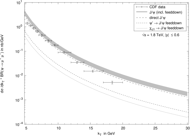
Figure 6: Unpolarized cross section $d\sigma/dk_{T}$ for $J/\psi$ production with contribution from all different channels and the combined error.

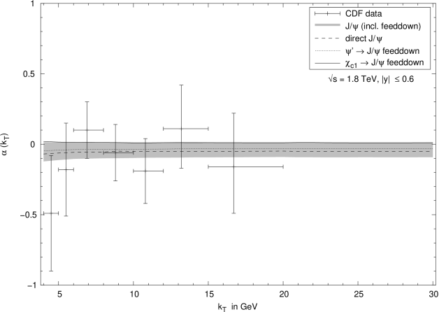
Figure 7: $\alpha$ for $J/\psi$ from $B$ decays with contributions from all different channels and the combined error.

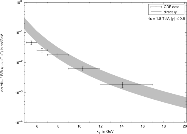
Figure 8: Unpolarized cross section $d\sigma/dk_{T}$ for $\psi^{\prime}$ production with the combined error.

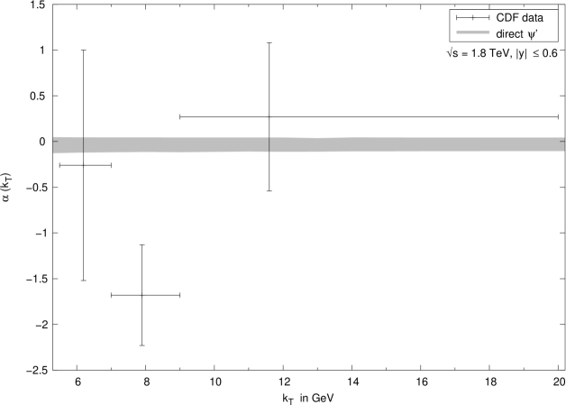
Figure 9: $\alpha$ for $\psi^{\prime}$ from $B$ decays with the combined error.

7.4 Final results

The final results for $J/\psi$ as well as the experimental data are presented in figures 6 and 7. The corresponding quantities for $\psi^{\prime}$, to which no feed-down channels contribute, are shown in figures 8 and 9.

The unpolarized $J/\psi$ cross section shows a good agreement with the experimental data [Abe:1997jz] within error bars at intermediate transverse momenta $k_{T}$. On the other hand it overestimates the data quite strongly for small and large $k_{T}$, a feature which is a result of extrapolating the $B$ cross section (see section 7.1 for details).

Our prediction for the polarization parameter $\alpha$ is consistent with $0$, but the central value prefers to be small and negative. For the higher transverse momentum range $k_{T}=10\ldots 30$ GeV, we have $\alpha=-0.04\pm 0.06$. We find a good agreement with experimental data [Affolder:2000nn], although one has to admit that the statistical experimental uncertainties are enormous and for some $k_{T}$ bins cover as much as one third of the theoretically allowed parameter space of $\alpha$. The prediction for $\alpha$ is almost independent of $k_{T}$ and only shows a slight decrease towards the lowest transverse momentum values displayed in figure 7. Also the central values of the experimental data exhibit such a tendency, but the decrease at low $k_{T}$ is much more significant. Even here the predictions lie within $1\sigma$ deviation of the experimental data.

Obviously on the basis of the current data it is not possible to constrain the values of the poorly determined color octet ${}^{1}S_{0}$ and ${}^{3}P_{0}$ matrix elements any further. Nevertheless, there are good prospects that the situation on the experimental side will improve in the near future. Run II of the Tevatron is in progress for one and a half years already and the $B$ physics group of the CDF collaboration expects to increase statistics effectively by a factor of 50 [Anikeev:2001rk]. This will reduce the statistical error at least in the low and medium transverse momentum range significantly and also data in higher $k_{T}$ bins will become available. Hence it is expected that after Run II only systematical errors will dominate the uncertainties of the $\alpha$ measurement [Anikeev:2001rk]. Even if those will not be improved, $\alpha$ will have an error of the order of $\sim 0.02$, enough to exclude a good part of the numerical ranges of the matrix elements.

Since our calculation can be equally applied to $\psi^{\prime}$ production without significant modifications, we have extended the analysis to this charmonium state. For intermediate and large values of $k_{T}$ the unpolarized cross section in figure 8 agrees with the CDF data within error bars. The reason for the excess at low $k_{T}$ is the same as in the case of $J/\psi$ discussed earlier. With $\alpha=-0.03\pm 0.07$ for $k_{T}=10\ldots 30$ GeV, the polarization parameter for $\psi^{\prime}$ does not differ significantly from the one for $J/\psi$, but here a comparison with data is almost impossible as can be seen from figure 9. The situation is worse than for $J/\psi$, because the error bars are huge and one of the data points even lies outside the allowed region for $\alpha$, which is restricted to the interval $[-1,+1]$ for theoretical reasons. On the other hand, once more precise data will be available, to derive tighter constraints on the $\psi^{\prime}$ matrix elements will be more straight forward than for $J/\psi$, because all $\psi^{\prime}$ are directly produced from $B$ decays, since no feed-down channels are known to contribute.

8 Summary and conclusions

In this paper, using the NRQCD formalism and the PM, we have calculated the semi-inclusive decay rate, $\Gamma(B\to J/\psi+X)$ with polarized $J/\psi$ as final states. Subsequently these results were generalized to the case of other $J=1$ quarkonium states, i.e., $\psi^{\prime}$ and $\chi_{c1}$. The results were applied to the Fermilab Tevatron setup. In this case, we calculated the differential cross sections for unpolarized $J/\psi$ and $\psi^{\prime}$ production in $B$ decays and, the polarization parameter $\alpha$ for $J/\psi$ and $\psi^{\prime}$, originating from $B$ decays. The $B$ meson production cross section in $p\bar{p}$ collisions at the Tevatron was implemented by a phenomenological fit to the CDF data [Affolder:2000nn]. We considered the feed-down from $\psi^{\prime}$ and $\chi_{c1}$ for $J/\psi$ production. To obtain a meaningful comparison of our predictions with experimental data, we carried out a detailed analysis of the various theoretical uncertainties involved. In particular, it was shown that $\alpha$ is almost not influenced by most input parameters, except for the matrix elements and the distribution function parameter, $\varepsilon_{P}$. Therefore, for an extraction of this parameter, it is pertinent for more precise numerical values of the matrix elements, especially, the poorly determined $\langle{\cal O}_{8}^{\psi}(^{1}S_{0})\rangle$ and $\langle{\cal O}_{8}^{\psi}(^{3}P_{0})\rangle$.

To perform such an improved fit of these non-perturbative matrix elements, the precision of the data has to be increased significantly which is also expected in Run II of the Tevatron. Furthermore, it would also be desirable to experimentally separate direct $J/\psi$ production from the feed-down channels. This restricts the uncertainties, simply because the number of relevant matrix elements get reduced . Theoretically, an inclusion of higher order corrections would be preferable to reduce the errors due to factorization scale dependence, in particular that of the color singlet Wilson coefficient. Since it is known that this cannot be achieved at next-to-leading order, a next-to-next-to-leading order calculation might be necessary [Beneke:1998ks]. Also, a better knowledge of $\varepsilon_{P}$ would improve the precision of $\alpha$. For $\psi^{\prime}$ this could be accomplished with a fit to the unpolarized momentum spectrum of $\psi^{\prime}$ in $B$ decays to more accurate CLEO [Anderson:2002jf] and BaBar [Aubert:2002yk] data that have become available very recently. The feed-down channels and resonant two body final states ($J/\psi+K$ and $J/\psi+K^{\star}$) complicate such a fit for $B\to J/\psi+X$. Additionally, it might be worth to try a different parameterization for the heavy quark distribution function, because in $b$ fragmentation, which serves as a motivation for the distribution function, the Peterson form might not be appropriate [Cacciari:2002pa].

A significant reduction of the matrix element errors is mostly likely to be achieved with the help of a global fit. Among the processes that could contribute to this fit, $\alpha$ from $B$ decays might play an important role, being one of the few quantities that is sensitive to the individual values of the $\langle{\cal O}_{8}^{\psi}(^{1}S_{0})\rangle$ and $\langle{\cal O}_{8}^{\psi}(^{3}P_{0})\rangle$ matrix elements.

Acknowledgments

This work has been supported by the Bundesministerium für Bildung, Wissenschaft, Forschung und Technologie, Bonn under contract no. 05HT1PEA9. We wish to thank E.A. Paschos for suggesting this problem and for many useful discussions.

Appendix A Appendix

A.1 NRQCD Matrix Elements

Here, we present numerical values of the matrix elements from the literature that are required in our analysis. The tables below are structured as follows. Apart from the numerical value, including statistical as well as systematical errors (wherever given) we refer to the method/process that has been used to extract them and the corresponding references to the original publications. This list only provides an overview of the numerical values that we have considered in our analysis and is by no means meant to be exhaustive. In the last line of each table we give a range for the corresponding matrix element that we have used in our calculation as described in section 6.3.

A.1.1 $J/\psi$ Matrix Elements

$\vphantom{\Big{(}\Big{)}}\langle{\cal O}_{1}^{J/\psi}(^{3}S_{1})\rangle$ in GeV${}^{3}$	method/process	Reference
$0.994\pm 0.002^{+0.204}_{-0.145}$	lattice calculation	[Bodwin:1996tg]
$1.16$	Buchmüller-Tye potential	[Eichten:1995ch]
$1.1\pm 0.1$	$J/\psi\to e^{+}e^{-}$	[Groom:2000in]
$0.763\pm 0.054$	$J/\psi\to e^{+}e^{-}$ (without QCD)	[Kniehl:1998qy]
$1.3\pm 0.1$	$J/\psi\to e^{+}e^{-}$ (incl. LO QCD)	[Kniehl:1998qy, Braaten:1999qk]
$1.1\pm 0.1$

$\vphantom{\Big{(}\Big{)}}\langle{\cal O}_{8}^{J/\psi}(^{3}S_{1})\rangle$ in $10^{-3}$ GeV${}^{3}$	method/process	Reference
$6.6\pm 2.1$	hadroproduction (CDF data)	[Cho:1996vh, Cho:1996ce]
$3.94\pm 0.63$	hadroproduction (CDF data)	[Kniehl:1998qy]
$10.6\pm 1.4^{+10.5}_{-5.9}$	hadroproduction (CDF data)	[Beneke:1997yw]
$9.6\pm 1.5$	hadroproduction (CDF data)	[Sanchis-Lozano:1999um]
$4.4\pm 0.7$	hadroproduction (CDF data)	[Braaten:1999qk]
$6.0\pm 3.0$

$\vphantom{\Big{(}\Big{)}}M_{r}^{J/\psi}$ in $10^{-2}$ GeV${}^{3}$	$r$	method/process	Reference
$6.6\pm 1.5$	$3$	hadroproduction (CDF data)	[Cho:1996vh, Cho:1996ce]
$6.52\pm 0.67$	$3.47$	hadroproduction (CDF data)	[Kniehl:1998qy]
$3.0$	$7$	hadroproduction (fixed target)	[Beneke:1996tk]
$8.7\pm 0.9$	$3.4$	hadroproduction (CDF data)	[Braaten:1999qk]
$2.0$	$7$	photoproduction	[Fleming:1997jx]
$4.38\pm 1.15^{+1.52}_{-0.74}$	$3.5$	hadroproduction (CDF data)	[Beneke:1997yw]
$1.5$	$3.1$	$Br(B\to J/\psi+X)$ (CLEO data)	[Beneke:1998ks]
$1.32\pm 0.21$	3	hadroproduction (CDF data)	[Sanchis-Lozano:1999um]
$5.0\pm 4.0$	$3.5$

$\vphantom{\Big{(}\Big{)}}\langle{\cal O}_{8}^{J/\psi}(^{1}S_{0})\rangle$ in $10^{-2}$ GeV${}^{3}$	method/process	Reference
$4.0$	leptoproduction	[Fleming:1997jx]
$14.5$	$Br(B\to J/\psi+X)$ (CLEO data)	[Kniehl:1999vf]
$6.5\pm 5.5$

$\vphantom{\Big{(}\Big{)}}\langle{\cal O}_{8}^{J/\psi}(^{3}P_{0})\rangle$ in $10^{-2}$ GeV${}^{5}$	method/process	Reference
$-0.3\cdot m_{c}^{2}$	leptoproduction	[Fleming:1997jx]
$-5.51$	$Br(B\to J/\psi+X)$ (CLEO data)	[Kniehl:1999vf]
$-4.0\pm 6.0$

A.1.2 $\psi^{\prime}$ Matrix Elements

$\vphantom{\Big{(}\Big{)}}\langle{\cal O}_{1}^{\psi^{\prime}}(^{3}S_{1})\rangle$ in GeV${}^{3}$	method/process	Reference
$0.440\pm 0.043$	$\psi^{\prime}\to e^{+}e^{-}$ (incl. LO QCD)	[Kniehl:1999vf]
$0.65\pm 0.6$	$\psi^{\prime}\to e^{+}e^{-}$ (incl. NLO QCD)	[Braaten:1999qk]
$0.76$	Buchmüller-Tye potential	[Eichten:1995ch]
$0.11$	leptonic decay rate	[Braaten:1995vv]
$0.6\pm 0.2$

$\vphantom{\Big{(}\Big{)}}\langle{\cal O}_{8}^{\psi^{\prime}}(^{3}S_{1})\rangle$ in $10^{-3}$ GeV${}^{3}$	method/process	Reference
$6.20\pm 0.95$	hadroproduction (CDF data)	[Kniehl:1999vf]
$4.2$	hadroproduction (CDF data)	[Braaten:1995vv]
$4.6\pm 1.0$	hadroproduction (CDF data)	[Cho:1996vh, Cho:1996ce]
$4.4\pm 0.8^{+4.3}_{-2.4}$	hadroproduction (CDF data)	[Beneke:1997yw]
$4.2\pm 1.0$	hadroproduction (CDF data)	[Braaten:1999qk]
$5.5\pm 2.5$

$\vphantom{\Big{(}\Big{)}}M_{r}^{\psi^{\prime}}$ in $10^{-2}$ GeV${}^{3}$	$r$	method/process	Reference
$1.8\pm 0.6$	$3$	hadroproduction (CDF data)	[Cho:1996vh, Cho:1996ce]
$1.79\pm 0.51$	$2.56$	hadroproduction (CDF data)	[Kniehl:1999vf]
$1.8\pm 0.56^{+0.62}_{-0.30}$	$3.5$	hadroproduction	[Beneke:1997yw]
$0.52$	$7$	hadroproduction (fixed target)	[Beneke:1996tk]
$1.3\pm 0.5$	$3.5$	hadroproduction (CDF data)	[Braaten:1999qk]
$0.6$	$3.1$	$Br(B\to\psi^{\prime}+X)$ (CLEO data)	[Beneke:1998ks]
$1.75\pm 1.25$	$3.0$

$\vphantom{\Big{(}\Big{)}}\langle{\cal O}_{8}^{\psi^{\prime}}(^{1}S_{0})\rangle$ in $10^{-2}$ GeV${}^{3}$	method/process	Reference
$-0.96$	$Br(B\to J/\psi+X)$ (CLEO data)	[Kniehl:1999vf]
$2.5\pm 2.5$

$\vphantom{\Big{(}\Big{)}}\langle{\cal O}_{8}^{\psi^{\prime}}(^{3}P_{0})\rangle$ in $10^{-2}$ GeV${}^{5}$	method/process	Reference
$2.58$	$Br(B\to J/\psi+X)$ (CLEO data)	[Kniehl:1999vf]
$0.0\pm 10.0$

A.1.3 $\chi_{cJ}$ Matrix Elements

$\vphantom{\Big{(}\Big{)}}\langle{\cal O}_{1}^{\chi_{c0}}(^{3}P_{0})\rangle$ in $10^{-2}$ GeV${}^{5}$	method/process	Reference
$4.8\cdot m_{c}^{2}$	Buchmüller-Tye potential	[Eichten:1995ch]
$4.4\cdot m_{c}^{2}$	Buchmüller-Tye potential	[Eichten:1995ch, Beneke:1996tk]
$22.9\pm 2.5$	hadroproduction (CDF data)	[Kniehl:1998qy]
$8.8\pm 2.13$	hadronic $\chi_{cJ}$ decays	[Bodwin:1992qr]
$8.9\pm 1.3$	$\chi_{c2}\to\gamma\gamma$	[Braaten:1999qk]
$6.0\pm 4.0$

$\vphantom{\Big{(}\Big{)}}\langle{\cal O}_{8}^{\chi_{c0}}(^{3}S_{1})\rangle$ in $10^{-3}$ GeV${}^{3}$	method/process	Reference
$4.5\ldots 6.5$	$B\to\chi_{c2}+X$	[Beneke:1998ks]
$0.681\pm 0.175$	hadroproduction (CDF data)	[Kniehl:1998qy]
$3.2\pm 1.4$	$\Gamma(B\to\chi_{c2}+X)/\Gamma(B\to e\nu_{e}+X)$	[Braaten:1995vv]
$1.39\pm 0.17$	hadroproduction (CDF data)	[Kniehl:1999vf]
$2.3\pm 0.3$	hadroproduction (CDF data)	[Braaten:1999qk]
$3.5\pm 3.0$

References

- [1] W.E.CaswellandG.P.Lepage, Phys.Lett.B167,437(1986).
- [2] T.A.DeGrandandD.Toussaint, Phys