IFUSP-DFN/02-077 IFT-P.060/2002 MADPH-02-1306
Measuring the Spectra of High Energy Neutrinos with a Kilometer-Scale Neutrino Telescope

Abstract

We investigate the potential of a future kilometer-scale neutrino telescope such as the proposed IceCube detector in the South Pole, to measure and disentangle the yet unknown components of the cosmic neutrino flux, the prompt atmospheric neutrinos coming from the decay of charmed particles and the extra-galactic neutrinos, in the 10 TeV to 1 EeV energy range. Assuming a power law type spectra, $d\phi_{\nu}/dE_{\nu}\sim\alpha E_{\nu}^{\beta}$, we quantify the discriminating power of the IceCube detector and discuss how well we can determine magnitude ($\alpha$) as well as slope ($\beta$) of these two components of the high energy neutrino spectrum, taking into account the background coming from the conventional atmospheric neutrinos.

I Introduction

Large volume neutrino telescopes are being constructed to detect high-energy neutrinos primarily from cosmologically distant sources. A major challenge for these experiments will be separating the contributions coming from the different sources in the observed flux. In this paper, we consider three different origins for high-energy neutrinos: conventional atmospheric neutrinos coming from the decay of charge pions and kaons, prompt atmospheric neutrinos from the decay of charmed particles and neutrinos from extra-galactic sources.

Of these sources, only the conventional atmospheric neutrino flux has been observed in the energy range from sub-GeV up to $\sim$ TeV range atmnuobs . Currently, the conventional atmospheric neutrino flux is known to about 15-20% review-atm . The other two fluxes, although anticipated by theoretical expectations, are experimentally unknown to us, and their observation will be extremely important.

Up to about $E_{\nu}\sim 100$ TeV the main source of atmospheric neutrinos is the decay of pions and kaons produced in the interactions of cosmic rays in the Earth atmosphere. At higher energies, these mesons will interact rather than decay, making the semileptonic decay of charmed particles the dominant source of atmospheric neutrinos. This gives rise to the so called prompt atmospheric neutrino flux which is, unfortunately, subject to large theoretical uncertainties. The uncertainties in the calculation of the prompt neutrino fluxes reflect not only our poor knowledge of the atmospheric showering parameters, which for a given model can cause a change of an order of magnitude in the fluxes, but are mostly related to the model used to describe charm production at high energies, which is responsible for a discrepancy up to two orders of magnitude in the predictions costa . Typically, the energy dependence of prompt neutrino flux is $d\phi_{\nu}/dE_{\nu}\sim E_{\nu}^{-3}$.

If the prompt atmospheric neutrino flux can be determined by experimental data, this can provide a unique opportunity to study heavy quark interactions at energies not accessible by terrestrial accelerators. Furthermore, the characterization of the prompt component of the neutrino flux will enhance the discriminating power of the other components at higher energies.

High energy neutrinos are also expected to be produced in astrophysical sources at cosmological distances. The most conventional source candidates are compact objects such as gamma ray bursts grb and active galactic nuclei jets, called blazars agn . In these sources, neutrinos may be generated via pion production in the collision between protons and photons in highly relativistic shocks. A typical energy dependence of the extra-galactic neutrino flux in these scenarios is $d\phi_{\nu}/dE_{\nu}\sim E_{\nu}^{-2}$. For other possibile extra-galactic neutrino spectra, see, for example, dmitry .

Other possible sources of extra-galactic neutrinos include neutrinos generated in the annihilation of weakly interacting massive particles wimps , the propagation of ultra-high energy protons cosmogenic or in a variety of top-down scenarios including decaying or annihilating superheavy particles with GUT-scale masses shparticles , decaying topological defects defects , the so-called Z-burst mechanism z or Hawking radiation from primordial black holes hawking . The neutrino fluxes from compact sources, the propagation of ultra-high energy protons or top-down scenarios can be tied to the observed cosmic ray flux. Since a myriad of speculations exist, resolution will likely be reached only by experiment. Currently, only the upper bound on such high energy extra-galactic neutrino flux, $E_{\nu}^{2}d\phi_{\nu}/dE_{\nu}\raise 1.29167pt\hbox{$\;<$\kern-7.5pt\raise-4.73611pt\hbox{$\sim\;$}}10^{-5}$ GeV cm^-2 s^-1 sr^-1, has been obtained amandacascade . For a review of high-energy neutrino sources and detection, see review .

Many important questions regarding the origin of cosmic rays can be decided by neutrino observations. The determination of an extra-galactic neutrino flux will be very important for understanding the nature of the sources of the ultra-high energy cosmic rays.

We investigate the possibility of determining the prompt atmospheric neutrino and the extra-galactic neutrino energy spectra (slope and magnitude) using down-going showers cascade ; amandacascade induced by neutrinos in a kilometer-scale neutrino telescope conceived to detect high-energy neutrinos at high rates, such as IceCube, particularly in the region $10\mbox{ TeV }\raise 1.29167pt\hbox{$\;<$\kern-7.5pt\raise-4.73611pt\hbox{$\sim\;$}}E_{\nu}\raise 1.29167pt\hbox{$\;<$\kern-7.5pt\raise-4.73611pt\hbox{$\sim\;$}}1\mbox{ EeV}$. We demonstrate that since the energy spectra of these two neutrino fluxes are expected to be rather different, by using shower events from which one can reconstruct the initial neutrino energy with some accuracy, IceCube will be able to determine their energy spectra separately even if they co-exist.

The organization of this paper is as follows. In Sec. II, we briefly describe the presumed detector setup as well as the type of neutrino events we will consider. In Sec. III, we describe the analysis method and in Sec. IV we present our results. Finally, Sec. V is devoted to discussions and conclusions.

II Neutrino-Induced Shower Events in a Neutrino Telescope

We will assume a kilometer-scale detector with excellent energy and angular resolution, such as the IceCube project at the South Pole icecube , where strings of photo-multiplier tubes are distributed throughout a natural Cherenkov medium, ice.

We are not going to be interested for our analysis in muon events since we need to be able to determine the parent neutrino energy with some precision; we will rather look at shower events. We are interested in neutrinos in the energy range from 10 TeV to 1 EeV, so we will consider all neutrinos ($\nu_{e}$,$\nu_{\mu}$,$\nu_{\tau}$) which interact via charged or neutral current interactions within or close to the detector volume and produce a shower which can be observed by the detector.

We restrict our analysis to showers induced by down-going neutrinos, so we do not have to worry about energy losses and absorption in the Earth and be equally sensitive to all neutrino flavors. We assume that the detector will be able to reconstruct the parent neutrino energy from the collected shower energy within a factor of about 2-3, so that the data spanning five decades in energy can be subdivide into the following five energy bins $\Delta E_{\nu}=[10^{4}-10^{5},10^{5}-10^{6},10^{6}-10^{7},10^{7}-10^{8},10^{8}-10^{9}]$ GeV.

The only background comes from showers induced by conventional atmospheric neutrinos, which will only play a role in the first two energy bins. This background can be, in principle, substantially reduced if we consider only showers initiated by neutrinos with zenith angle greater than 30 degrees above the horizon, since the conventional atmospheric neutrino flux is peaked in this direction, while prompt and extra-galactic neutrinos have approximately flat zenith angle distributions. Another possible way to reduce the background level is to eliminate shower events which are accompanied by a muon track due to charged current interactions of $\nu_{\mu}$ with the ice. At these energies the conventional atmospheric neutrino flux is mostly $\nu_{\mu}$ while the prompt and extra-galactic neutrino fluxes are also expected to present a large amount of $\nu_{e}$ and $\nu_{\tau}$. The ratio of showers to muon tracks at a given zenith angle can also be used as a way to deplete the number of background events. We mention these as possible improvements to our results, but will not attempt to implement them here since this type of calculations highly depends on the shower angular resolution, detector acceptances and efficiencies which are currently unknown.

We estimate the number of neutrino-induced showers in the $i$-th bin, $N_{i}$, in a kilometer-scale detector simply by

$$N_{i}=\displaystyle A\int_{\Delta E_{\nu}^{i}}\frac{d\phi_{\nu}}{dE_{\nu}}\,\sigma_{\nu}(E_{\nu})dE_{\nu}\,d\Omega,$$ (1)

where $A=N_{A}\times T\times V\times\rho$, $N_{A}$ being the Avogadro’s number, $T$ the exposure time of observation, $V$ the detector effective volume (assumed to be 1 km³) $\rho\sim 1$ g/cm³, the ice density. The neutrino interaction cross section gandhi , $\sigma_{\nu}$, includes charged and neutral current contributions and the neutrino flux. $d\phi_{\nu}/dE_{\nu}$ will vary according to our theoretical assumptions for the flux energy dependence. Integration over the upper hemisphere as well as average in each energy bin is implied.

We parametrize the extra-galactic or the prompt neutrino flux spectrum by two parameters $(\alpha,\beta)$ as,

$$\frac{d\phi_{\nu}}{dE_{\nu}}\equiv\alpha\left(\frac{E_{\nu}}{E_{0}}\right)^{\beta},$$ (2)

where we fixed $E_{0}=1$ GeV and $\alpha$ is defined to be given in units of GeV^-1 cm^-2 s^-1 sr^-1 throughout this paper. Roughly speaking, it is expected that, $\beta\sim-2$ and $-3$ for extra-galactic and prompt atmospheric neutrino flux, respectively. In this work, we assume that we do not know, a priori, the spectrum index but try to determine it experimentally.

For the calculations of the number of conventional atmospheric neutrino shower events in the $i$-th bin, $N_{i}^{\text{atm}}$, we substitute $d\phi_{\nu}/dE_{\nu}$ in Eq. (1) by the Bartol flux nuflux which will be considered to be the reference conventional atmospheric neutrino flux in this paper.

III Analysis Method

In order to quantify the discriminating power of IceCube type detectors to different flux models, we use the $\chi^{2}$ function which is defined as

$$\chi^{2} \equiv \displaystyle\sum_{i=1}^{2}\frac{\left(N_{i}^{\text{th}}-N_{i}^{\text{obs}}\right)^{2}}{N_{i}^{\text{obs}}+N_{i}^{\text{atm}}+(\sigma_{\text{atm}}N_{i}^{\text{atm}})^{2}}$$ (3)

$$+ 2\times\sum_{i=3}^{5}\left\{N_{i}^{\text{th}}-N_{i}^{\text{obs}}+N_{i}^{\text{obs}}\ln[N_{i}^{\text{obs}}/N_{i}^{\text{th}}]\right\},$$

where $N_{i}^{\text{th}}=N_{i}(\alpha_{\text{EG}},\beta_{\text{EG}}),N_{i}(\alpha_{\text{prompt}},\beta_{\text{prompt}})$ or the sum, $N_{i}^{\text{obs}}=N_{i}(\alpha^{0}_{\text{EG}},\beta^{0}_{\text{EG}}),N_{i}(\alpha^{0}_{\text{prompt}},\beta^{0}_{\text{prompt}})$ or the sum, and the energy bins, with energy varied from 10 TeV to 1 EeV, are as defined in Sec. II. Note that the $\chi^{2}$ will be either a function of two or four variables.

The conventional atmospheric neutrino flux has to be considered as a background to the observation of any other component up to $E_{\nu}\sim 1$ PeV. We assume the conventional atmospheric flux prediction can be subtracted from the data and include the statistical ($\sqrt{N_{i}(\alpha^{0},\beta^{0})}$ and $\sqrt{N_{i}^{\text{atm}}}$) as well as the systematical ($\sigma_{\text{atm}}N_{i}^{\text{atm}}$) uncertainties coming from this data in the $\chi^{2}$ for the first two bins. We note that $\sigma_{\text{atm}}$ indicates the theoretical uncertainty in the absolute normalization of the conventional atmospheric neutrino flux which can be significantly reduced by future measurements.

The analysis strategy we propose is the following. In the future, when data exists, the spectrum should be first fitted with a single power law type spectrum. If it can be well fitted by such a power law with $\beta\sim-2$ $(-3)$ we will be able to conclude that the data is most likely dominated by extra-galactic (prompt atmospheric) neutrinos. If they can not be well fitted by a single power law spectrum, the next step should be to fit them with two components with different power laws.

Since we do not yet have sufficient data, we will simulate an experimental data set which either have pure or dominant extra-galactic, pure or dominant prompt or a combination of extra-galactic and prompt neutrino components. Then we will perform a $\chi^{2}$ fit to see if we can correctly reproduce the input values, without any assumption about these parameters.

For a given input, we first try to fit the simulated data with a single component, i.e., by minimizing $\chi^{2}(\alpha,\beta)$. If this fit is not very good, $\chi^{2}_{\text{min}}\raise 1.29167pt\hbox{$\;>$\kern-7.5pt\raise-4.73611pt\hbox{$\sim\;$}}11.8$, then we try to perform a two component fit, i.e., by minimizing $\chi^{2}(\alpha_{\text{EG}},\beta_{\text{EG}},\alpha_{\text{promt}},\beta_{\text{prompt}})$. After minimizing the $\chi^{2}$ function, we calculate the allowed region in the $\alpha\times\beta$ plane by imposing $\chi^{2}(\alpha,\beta)=\chi^{2}_{\text{min}}+11.8$, which corresponds to a 3 $\sigma$ level estimation.

IV A Three Prong View of the Problem

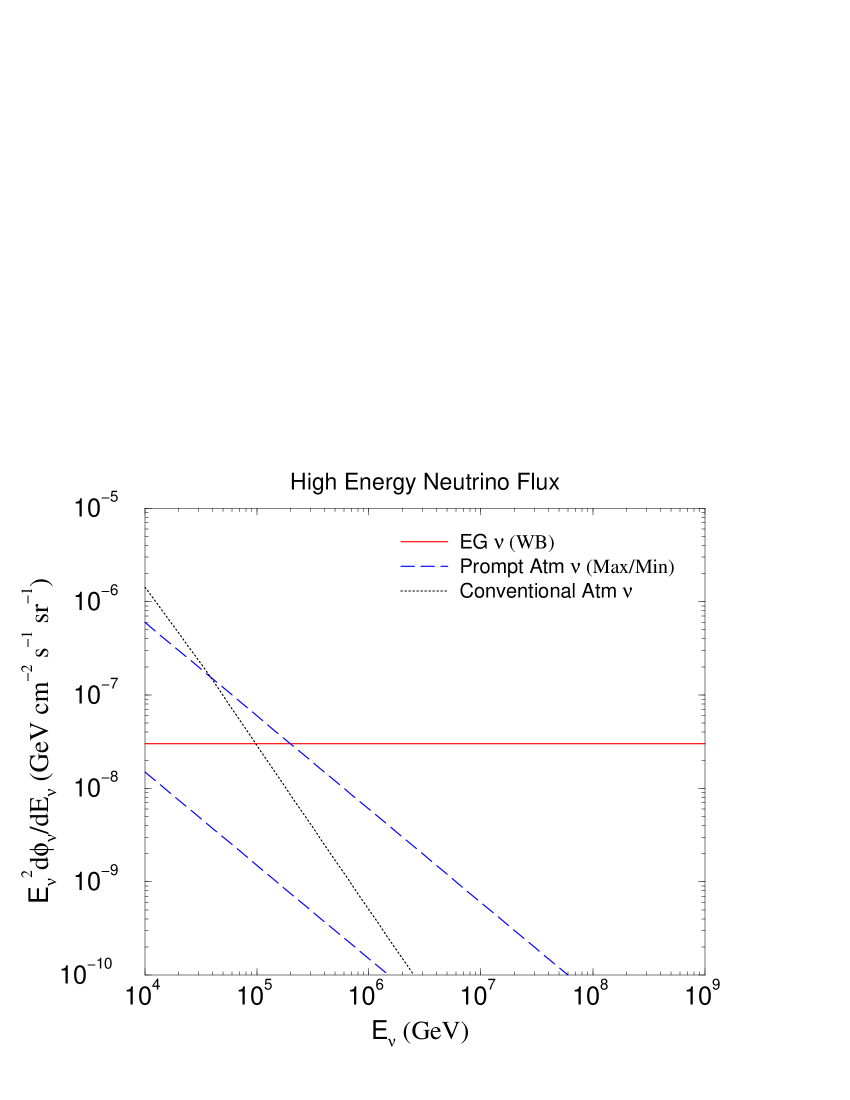
Figure 1: The three kind of high energy neutrino fluxes that are considered in this paper: conventional atmospheric neutrinos (dotted line), the Waxman-Bahcall (WB) flux for extra-galactic neutrinos (solid line) and prompt atmospheric neutrinos (region circumscribed by the dashed lines).

We first show in Fig. 1 the theoretical expectations for the three contributions to the neutrino flux we will be considering in this work. The conventional atmospheric neutrino flux has currently a theoretical uncertainty of about 15%. The prompt neutrino contribution is only known within 2 orders of magnitude, its minimum and maximum values are shown in the plot by the dashed lines, which rougly correspond to the range discussed in  costa . The Waxman-Bahcall (WB) flux WB , which is shown in the plot, will be considered to be our reference extra-galactic neutrino flux.

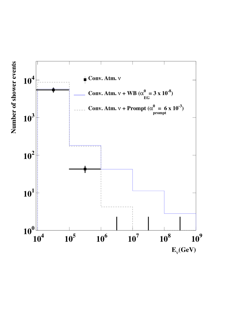
Figure 2: Number of down going shower events expected after 10 years of data taking in IceCube. The number of conventional atmospheric neutrino showers are shown with an error bar which includes the statistical as well as the systematic error with $\sigma_{\text{atm}}=15$%. Two values of assumed input $\alpha^{0}$’s are indicated in the plot in units of GeV^-1 cm^-2 s^-1 sr^-1.

We show in Fig. 2, the expected number of shower events for the neutrino fluxes presented in Fig. 1. As expected from Fig. 1, the contribution from conventional atmospheric neutrinos dominates in the 1st energy bin and then it drops very quickly as energy increases. Because of the weak slope ($\beta=-2$), the contribution from extra-galactic neutrinos drops slowly as the energy increases and the flux from prompt neutrinos drops faster than the flux from extra-galactic neutrinos but slower than that from the conventional atmospheric neutrinos. From this plot, we can anticipate that the energy spectra ($\beta$) of extra-galactic and prompt neutrinos can be determined experimentally with certain accuracy. Below, we will quantify the precision of the determination of the flux parameters for various cases.

IV.1 Assuming a Dominant Extra-Galactic Component in the Data

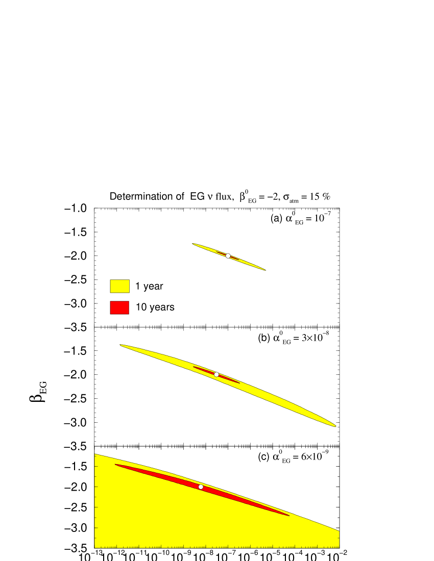
Figure 3: Determination of the parameters $(\alpha_{\text{EG}},\beta_{\text{EG}})$, after 1 and 10 years of IceCube observations, in the case the data is consistent with a dominant extra-galactic neutrino flux. We have assumed as an input $\beta^{0}_{\text{EG}}=-2$ and $\alpha^{0}_{\text{EG}}$(GeV^-1 cm^-2 s^-1 sr${}^{-1})=$ $10^{-7}$ (a), $3\times 10^{-8}$ (b) and $6\times 10^{-9}$ (c). The contours represent the determination at 3 $\sigma$ level. Contributions from the conventional atmospheric neutrinos are included in the $\chi^{2}$ with $\sigma_{\text{atm}}=15$%.

Let us first discuss the case where extra-galactic neutrino contribution is much larger than the prompt neutrino flux. In Fig. 3 we show how well the extra-galactic neutrino flux component can be determined by IceCube, after 1 and 10 years of data taking, for two other values of $\alpha^{0}_{\text{EG}}$ besides the reference WB ($\alpha^{0}_{\text{EG}}=3\times 10^{-8}$ GeV^-1 cm^-2 s^-1 sr^-1) one.

We have found that if the major component of the data are events induced by neutrinos coming from astrophysical sources, due to the difference in the slope of the conventional atmospheric neutrino flux and the extra-galactic flux, the first energy bin is only important for the determination of the flux parameters in the first year of data taking. After 10 years this contribution is completely irrelevant, which means that the events in the first bin can be completely ignored (a fit with four bins would be just as good), see Fig. 2 where we plot the number of shower events per energy bin. This also imply that our results are independent of the magnitude of the theoretical systematic error assumed for the conventional atmospheric neutrino calculation.

On the other hand, for the determination of the maximal sensitivity of IceCube, the background from conventional atmospheric events in the second bin is important and (see Fig. 2), in this case, there is some dependence on the value assumed for the systematic error.

We have calculated that after 10 years of observations, IceCube will be able to determine $\alpha_{\text{EG}}$ within an order of magnitude and $\beta_{\text{EG}}$ to $\approx$ 10%, assuming as input a dominant WB flux. We have also estimated that the maximal sensitivity of IceCube after 10 years of data taking to be $\alpha^{0}_{\text{EG}}\approx 6\times 10^{-9}$ GeV^-1 cm^-2 s^-1 sr^-1.

IV.2 Assuming a Dominant Prompt Component in the Data

Next let us consider the case where the prompt neutrino component is dominant. As can be seen in Fig. 2 the number of prompt neutrino shower events drops drastically after the second energy bin. This makes the determination of this flux, even if dominant over the extra-galactic flux, very sensitive to the theoretical uncertainty in the conventional atmospheric neutrino flux determination.

In fact, the flux determination will basically rely on the number of shower events in the first two energy bins. Since the 1st bin suffers from the background from the conventional atmospheric neutrino flux, we can only explore a relatively narrow range in $\alpha^{0}_{\text{prompt}}$ and, as a general rule, the parameters $\alpha_{\text{prompt}}$ and $\beta_{\text{prompt}}$ can be at most determined within 2 orders of magnitude and about 20%, respectively, with the present value of $\sigma_{\text{atm}}=$ 15%.

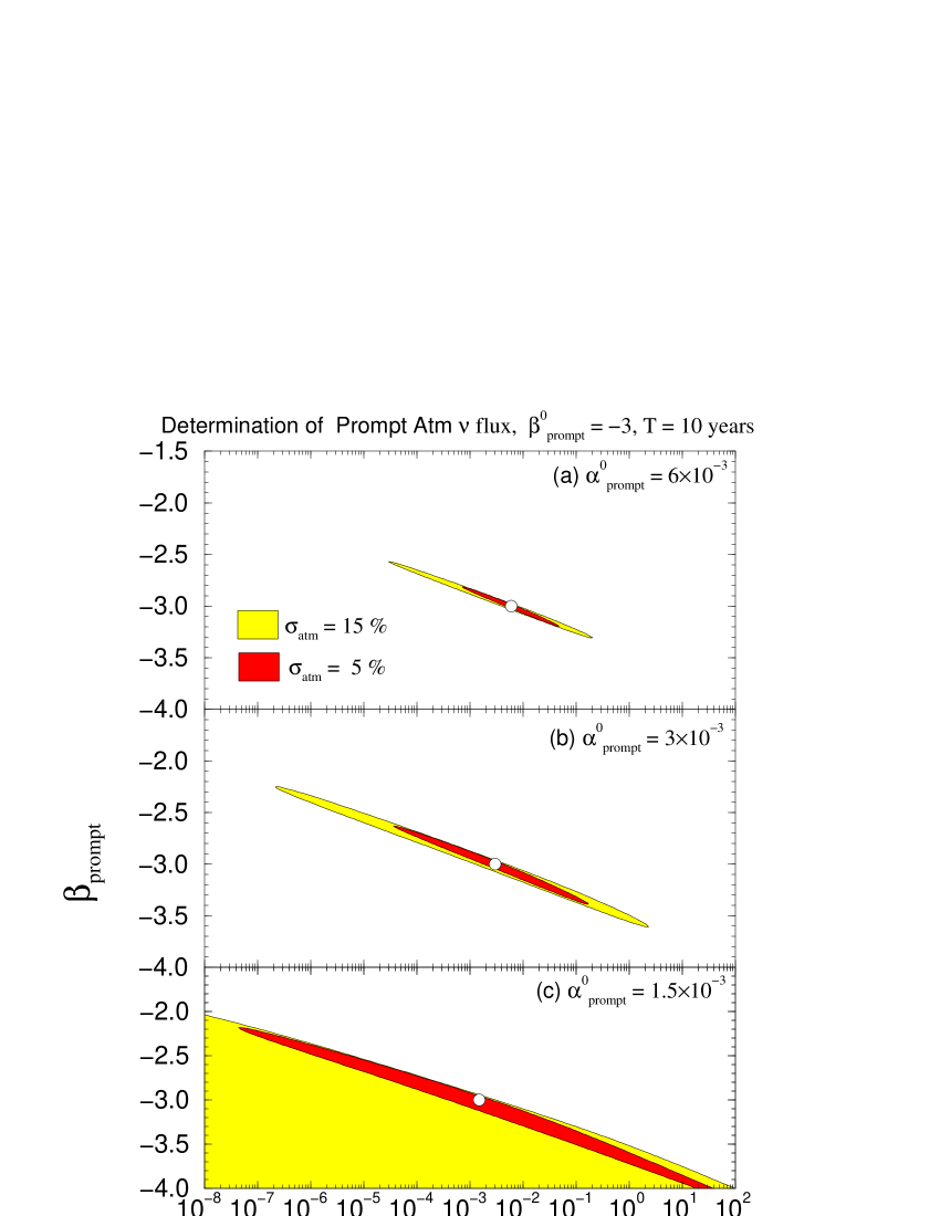
Figure 4: Determination of the parameters $(\alpha_{\text{prompt}},\beta_{\text{prompt}})$, after 10 years of IceCube observations, in the case the data is consistent with a dominant prompt neutrino flux. We have assumed as an input $\beta^{0}_{\text{prompt}}=-3$ and $\alpha^{0}_{\text{prompt}}$(GeV^-1 cm^-2 s^-1 sr${}^{-1})=$ $6\times 10^{-3}$ (a), $3\times 10^{-3}$ (b) and $1.5\times 10^{-3}$ (c). The contours are determined at 3 $\sigma$ level. Contributions from the conventional atmospheric neutrinos are included in the $\chi^{2}$ with $\sigma_{\text{atm}}=15$ and 5%.

To illustrate the effect of the systematical error $\sigma_{\text{atm}}$, we show in Fig. 4 how well the parameters of the prompt neutrino flux component can be determined by IceCube, after 10 years of data taking, for $\sigma_{\text{atm}}=$ 15 and 5% and for three possible values of $\alpha^{0}_{\text{prompt}}$ (GeV^-1 cm^-2 s^-1 sr^-1): (a) $6\times 10^{-3}$, which corresponds to the maximum allowed value by the theoretical calculations (see Fig. 1); (b)$3\times 10^{-3}$ and (c) $1.5\times 10^{-3}$, where we clearly reach the maximal sensitivity of IceCube.

IV.3 Disentangling Extra-galactic and Prompt Components

Finally, let us consider the case where both extra-galactic and prompt components give significant contributions. In order to determine whether it is possible to disentangle these two yet not measured components of the cosmic neutrino flux, if they are equally present in the data, we have investigated if it would be possible to fit the measured flux with a single power law assuming the data would be consistent with various values of $\alpha^{0}_{\text{EG}}$ and $\alpha^{0}_{\text{prompt}}$. We were able to compute the region in the ($\alpha^{0}_{\text{EG}},\alpha^{0}_{\text{prompt}}$) plane which cannot be explained by a single power law for different assumptions on $\sigma_{\text{atm}}$. This was done by projecting in this plane the 3 $\sigma$ level region which corresponds to $\chi^{2}_{\text{min}}(\alpha^{0}_{\text{EG}},\alpha^{0}_{\text{prompt}})+11.8$. This is shown in Fig. 5.

We see that for $\sigma_{\text{atm}}=$ 15%, $\alpha^{0}_{\text{EG}}=3\times 10^{-8}$ GeV^-1 cm^-2 s^-1 sr^-1 (our reference value) and $\alpha^{0}_{\text{prompt}}=6\times 10^{-3}$ GeV^-1 cm^-2 s^-1 sr^-1 (the maximal allowed value for the prompt neutrino flux) is a critical point, just on the boundary.

If the uncertainty in the overall normalization on the conventional atmospheric neutrino flux do not decrease by future measurements, this means that it will be very difficult to say anything definite about the prompt neutrino flux, assuming extra-galactic neutrinos also contribute to the data. In this case the two components will be indistinguishable and the extra-galactic neutrino flux will dominate the fit. For more optimistic values of $\sigma_{\text{atm}}$, the situation improves, so if $\sigma_{\text{atm}}=$ 5% can be achieved the prompt neutrino flux can be separated from the WB neutrino flux for $\alpha^{0}_{\text{prompt}}\raise 1.29167pt\hbox{$\;>$\kern-7.5pt\raise-4.73611pt\hbox{$\sim\;$}}2\times 10^{-3}$ GeV^-1 cm^-2 s^-1 sr^-1.

One would expect that an increase of $\alpha^{0}_{\text{EG}}$ with a corresponding decrease of $\alpha^{0}_{\text{prompt}}$ or a decrease of $\alpha^{0}_{\text{EG}}$ with a corresponding increase of $\alpha^{0}_{\text{prompt}}$ would help to separate the fluxes. This is in fact observed in Fig. 5. Nevertheless, as the extra-galactic neutrino flux increases, lower values of the prompt neutrino flux can be distinguished up to a minimum, where the prompt neutrino flux and the conventional atmospheric neutrino flux become virtually equal and indistinguishable as background. There is also a minimum value for the extra-galactic neutrino flux, below which the statistics are too low to be disentangled.

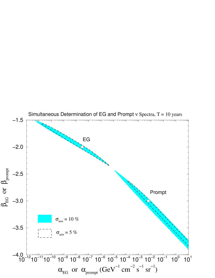
Figure 6: Same as Fig. 4, but in the case that the data have contributions from both prompt and extra-galactic neutrino fluxes. We have assumed as input $\beta^{0}_{\text{prompt}}=-3$, $\alpha^{0}_{\text{prompt}}=6\times 10^{-3}$ GeV^-1 cm^-2 s^-1 sr^-1 and $\beta^{0}_{\text{EG}}=-2$, $\alpha^{0}_{\text{EG}}=3\times 10^{-8}$ GeV^-1 cm^-2 s^-1 sr^-1, $\beta^{0}_{\text{EG}}=-2$. Contributions from the conventional atmospheric neutrinos are included in the $\chi^{2}$ with $\sigma_{\text{atm}}=10$% (shaded area) and 5% (area delimited by the dashed curves).

To illustrate the impact of $\sigma_{\text{atm}}$, we show in Fig. 6 how well the prompt and extra-galactic components can be determined by IceCube, after 10 years of data taking, for $\sigma_{\text{atm}}=$ 10 and 5%. In both cases the two components can be well separated, as expected from Fig. 5, but $\alpha_{\text{EG}}$, $\alpha_{\text{prompt}}$ will be determined within 3-4 orders of magnitude, $\beta_{\text{EG}}$ within about 20-30% and $\beta_{\text{prompt}}$ within about 20-40%.

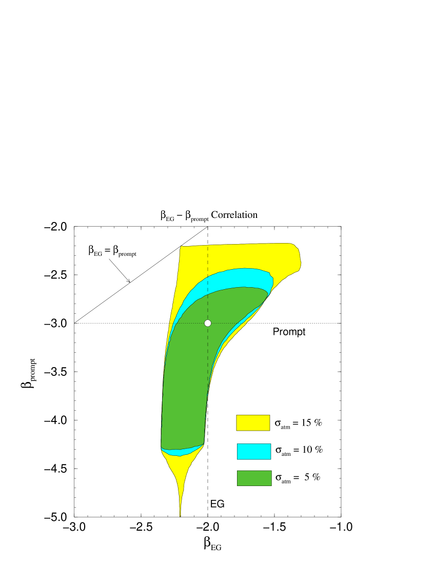
Figure 7: Allowed region in the ($\beta_{\text{EG}}$, $\beta_{\text{prompt}}$) plane for the same input values of Fig. 6. The contours are also determined at 3 $\sigma$ level. Contributions from the conventional atmospheric neutrinos are included in the $\chi^{2}$ with $\sigma_{\text{atm}}=$ 15, 10 and 5%.

For the critical point $\alpha^{0}_{\text{EG}}=3\times 10^{-8}$ GeV^-1 cm^-2 s^-1 sr^-1 and $\alpha^{0}_{\text{prompt}}=6\times 10^{-3}$ GeV^-1 cm^-2 s^-1 sr^-1 of Fig. 5 we have investigated the correlation between the determination of $\beta_{\text{EG}}$ and $\beta_{\text{prompt}}$, for $\sigma_{\text{atm}}=$ 15, 10 and 5%. In Fig. 7 we show the corresponding allowed regions projected in this plane. From this figure it is clear why at $\sigma_{\text{atm}}=$ 15% the single power law fit is still marginally acceptable. In this case the region allowed at 3 $\sigma$ touches the $\beta_{\text{EG}}=\beta_{\text{prompt}}$ line, so this possibility cannot be completely discarded. Any improvement on $\sigma_{\text{atm}}$ will place this point out of the allowed region, making the single power law fit unsuitable to explain the data.

V Discussions and Conclusion

We have investigated the possibility of future neutrino telescopes to separate the various contributions to the observed neutrino flux. We have considered that high-energy neutrinos from three different origins can contribute to the measured flux: conventional atmospheric neutrinos, prompt atmospheric neutrinos from the decay of charmed particles and neutrinos from extra-galactic sources.

We have restricted our analysis to showers induced by down-going neutrinos, not to have to worry about energy losses in the Earth and be equally sensitive to all neutrino flavors. We have also assumed the neutrino telescope will be able to reconstruct the parent neutrino energy from the collected shower energy within a factor of about 2-3.

Assuming the prompt atmospheric and extra-galactic neutrino fluxes can be described by a power law and parametrized by two parameters $\alpha$ (the magnitude) and $\beta$ (the slope), and considering that the conventional atmospheric neutrino flux is currently known with a theoretical uncertainty $\sigma_{\text{atm}}=$ 15%, our conclusion are the following.

If extra-galactic neutrinos constitute the dominant component of the measured flux, after 10 years of observations, a detector such as IceCube will be able to determine $\alpha_{\text{EG}}$ within an order of magnitude and $\beta_{\text{EG}}$ to $\approx$ 10%, assuming as input a dominant WB flux. This is independent of the conventional atmospheric neutrino contamination. We have also estimated that the maximal sensitivity of IceCube after 10 years of data taking will be $\alpha^{0}_{\text{EG}}\approx 6\times 10^{-9}$ GeV^-1 cm^-2 s^-1 sr^-1.

If prompt neutrinos constitute the dominant component of the measured flux, after 10 years, IceCube can determine $\alpha_{\text{prompt}}$ and $\beta_{\text{prompt}}$ at most within 2 orders of magnitude and about 20%, respectively, with the present value of $\sigma_{\text{atm}}=$ 15%. This can nevertheless be improved if this uncertainty can be substantially reduced. We also have estimated that in this case, the maximal sensitivity of IceCube will be achieved for $\alpha^{0}_{\text{prompt}}=1.5\times 10^{-3}$ GeV^-1 cm^-2 s^-1 sr^-1.

We have also determined in which cases a complete separation of the two components can be performed if both extra-galactic and prompt neutrinos contribute to the observed flux, Fig. 5 summarizes our conclusions on this. The main point here is that to clearly separate the prompt component from the extra-galactic component $\sigma_{\text{atm}}$ must be about 10% or less. If $\sigma_{\text{atm}}$ is much larger, a single power law will fit the data with an acceptable value of $\chi_{\text{min}}^{2}$.

Finally, let us mention that there is an additional signature that can be used to distinguish extra-galactic neutrinos from the prompt atmospheric ones. As first indicated by atmospheric neutrino data and lately confirmed by the K2K experiment K2K , $\nu_{\mu}$ oscillate to $\nu_{\tau}$ implying that one third of the total original extra-galactic $\nu$ flux will arrive at the Earth as $\nu_{\tau}$. On the other hand, prompt neutrinos are expected to have much lower $\nu_{\tau}$ than $\nu_{e}$ or $\nu_{\mu}$ content costa . For $E_{\nu}\raise 1.29167pt\hbox{$\;>$\kern-7.5pt\raise-4.73611pt\hbox{$\sim\;$}}1$ PeV a $\nu_{\tau}$ event can be clearly recognized through the observation a $\tau$, produced by a $\nu_{\tau}$ charge current interaction, which will decay in the detector. This gives rise to the so-called double-bang (when the $\tau$ is produced and decays within the detector volume) and lolly pop (when the $\tau$ is produced outside the detector but decays inside it) events review ; pakvasa . We estimate that after 10 years a detector like IceCube should observe, for the WB flux, a few such events, whereas no event is expected even for the maximal value of the allowed prompt neutrino flux.

Figure 5: Region in the $(\alpha^{0}_{\text{EG}},\alpha^{0}_{\text{prompt}})$ plane where the simulated data cannot be explained by a single power law for $\sigma_{\text{atm}}=$ 15, 10 and 5%, indicated by allows. The curves have been computed for $\chi^{2}=\chi^{2}_{\text{min}}+11.8$ (3 $\sigma$ level). The vertical and horizontal dashed lines cross at the critical point where $\alpha^{0}_{\text{EG}}$ takes the value for the WB flux and $\alpha^{0}_{\text{prompt}}$ takes the maximal allowed value for the prompt neutrino flux contribution in Fig. 1.