THEORY-MOTIVATED BENCHMARK MODELS AND SUPERPARTNERS AT THE TEVATRON

G. L. Kane¹, J. Lykken², Stephen Mrenna², Brent D. Nelson¹, Lian-Tao Wang¹ and Ting T. Wang¹

Recently published benchmark models have contained rather heavy superpartners. To test the robustness of this result, several benchmark models have been constructed based on theoretically well-motivated approaches, particularly string-based ones. These include variations on anomaly and gauge-mediated models, as well as gravity mediation. The resulting spectra often have light gauginos that are produced in significant quantities at the Tevatron collider, or will be at a 500 GeV linear collider. The signatures also provide interesting challenges for the LHC. In addition, these models are capable of accounting for electroweak symmetry breaking with less severe cancellations among soft supersymmetry breaking parameters than previous benchmark models.

Introduction

Benchmark models can be of great value in helping plan and execute experimental analyses. They allow quantitative studies of detector design and triggers, and can be important in setting priorities for experimental groups. They suggest what signatures can be the most fruitful search channels for finding new physics. For example, if benchmark models suggest rates and signatures that imply some kinds of new physics are unlikely to be seen compared to others, Ph.D. thesis topics and the associated experimental efforts may move in the direction indicated by those suggestions. Benchmark models can also provide essential guidance about what backgrounds are important to understand and what systematic errors need to be controlled. Consequently it is very important that the benchmark models not misrepresent the true physics situation. Finally, constructing benchmark models can also be valuable theoretical exercises, helping us to gain insight into which features of the theory imply certain phenomena and vice versa.

To be precise, we define a benchmark model as one in the framework of softly-broken supersymmetry and based on a theoretically motivated high scale approach. Currently, such models cannot be specified in sufficient detail to calculate a meaningful spectrum of interactions without making some assumptions or approximations – and these should be ones which make sense in the context of the theory.

In the past two years some benchmark models for supersymmetric spectra and signatures have been published [1, 2]. A general and perhaps surprising feature of these benchmarks is that the resulting superpartners are rather heavy, and in particular few or no superpartners are likely to be observed at the Tevatron collider. The published benchmark models are constructed using various assumptions. Such assumptions may or may not be true, and it is important to understand whether other approaches to benchmark models generally lead to such heavy spectra or not. One important concern with the published models is that they can be consistent with electroweak symmetry breaking (EWSB) only by having large cancellations between large contributions to $M_{Z}.$ That is a worrisome property [3], and leads one to question the relevance and implications of such models.

We have studied these issues and constructed several benchmark models that have good underlying theoretical motivation. We find that the resulting spectra typically do have some light superpartners that will be produced in significant quantities at the Tevatron or a $500~{}\mathrm{GeV}$ linear collider. Further, these models typically do describe EWSB without large cancellations, so perhaps their implications (including the opportunity to observe superpartners at the Tevatron) should be taken very seriously. In those cases where it is physically reasonable we have indicated which parameters can be varied to provided so-called “model lines.”

To be explicit, we propose seven sets of high–scale supersymmetry–breaking parameters as inputs to determine the weak–scale properties. All of these sets have a string theory basis, as is explained in Sections 1-3 of the paper. To summarize, the first set of benchmarks is motivated by nonperturbative methods of achieving dilaton stabilization leading to a reasonable minimum of the supersymmetry–breaking potential. They are specified by:

$${\rm Case\;A:}\qquad\left\{\tan\beta,\;m_{3/2},\;a_{\rm np}\right\} = \left\{10,\;1500~{}\mathrm{GeV},\;1/15.77\right\}$$ (1)

$${\rm Case\;B:}\qquad\left\{\tan\beta,\;m_{3/2},\;a_{\rm np}\right\} = \left\{5,\;3200~{}\mathrm{GeV},\;1/37.05\right\}$$ (2)

$${\rm Case\;C:}\qquad\left\{\tan\beta,\;m_{3/2},\;a_{\rm np}\right\} = \left\{5,\;4300~{}\mathrm{GeV},\;1/61.36\right\},$$ (3)

where $\tan\beta$ is the ratio of Higgs vacuum expectation values, $m_{3/2}$ is the gravitino mass, and $a_{\rm np}$ is related to the nonperturbative corrections to the dilaton potential. A possible model line is to vary the parameter $a_{\rm np}$ with all other parameters fixed. The next set of benchmark points are based on string models where the moduli fields are responsible for breaking supersymmetry. They are specified by $\tan\beta$, $m_{3/2}$, a Green-Schwarz coefficient $\delta_{\mathsc{gs}}$, and a moduli expectation value:

$${\rm Case\;D:}\qquad\left\{\tan\beta,\;m_{3/2},\;\delta_{\mathsc{gs}},\;\left\langle{\rm Re}\;t\right\rangle\right\} = \left\{45,\;20~{}\mathrm{TeV},\;-15,\;1.10\right\}$$ (4)

$${\rm Case\;E:}\qquad\left\{\tan\beta,\;m_{3/2},\;\delta_{\mathsc{gs}},\;\left\langle{\rm Re}\;t\right\rangle\right\} = \left\{30,\;20~{}\mathrm{TeV},\;-9,\;1.23\right\}.$$ (5)

A possible model line is to vary $\left\langle{\rm Re}\;t\right\rangle$ for a given value of $\delta_{\mathsc{gs}}$. The last set of benchmarks points are based on the idea of partial gauge–mediation arising from high–scale fields, and are specified by $\tan\beta$, $m_{3/2}$ and the SM quantum numbers of the high–scale fields:

$${\rm Case\;F:}\qquad\left\{\tan\beta,\;m_{3/2},\;n_{D},\;n_{L},\;N_{1}\right\}=\left\{10,\;120~{}\mathrm{GeV},\;4,\;0,\;(3/5)\right\}$$ (6)

$${\rm Case\;G:}\qquad\left\{\tan\beta,\;m_{3/2},\;n_{D},\;n_{L},\;N_{1}\right\}=\left\{20,\;130~{}\mathrm{GeV},\;3,\;0,\;(3/5)\right\}.$$ (7)

A possible model line is the variation of quantum numbers, in particular the hypercharge $N_{1}$. The corresponding values of the “usual” soft terms are collected for all the benchmark points in Table 1 in Section 4. The reader interested mainly in the phenomenological implications of these benchmarks may proceed directly to that point, especially on a first reading. The appropriate input parameters to the PYTHIA event generator are also available [4].

Most previous benchmarks were based on the so-called Constrained Minimal Supersymmetric Standard Model (cMSSM) which is characterized by universal values $m_{0}$ for the soft scalar masses, a universal gaugino mass denoted $m_{1/2}$ and a universal trilinear scalar coupling $A_{0}$ [5, 6, 7, 8, 9, 10, 11], subjected to theoretical and experimental constraints. These models are quite simple and well defined, and could once rightly claim to represent the state of the art in effective theory constructions motivated by string theory. But recent progress in realistic low-energy effective models, coupled with the recently obtained one loop expressions for soft terms in supergravity theories derived from strings [12], suggests that this universal paradigm may not accurately reflect the underlying string theory. In addition, phenomenological constraints that may not hold have been imposed on these benchmark models, such as insisting that they provide the entire cold dark matter of the universe with the needed relic density arising only from thermal production mechanisms.

The phenomenology of cMSSM models is largely generic. Once gaugino mass degeneracy is enforced experimental limits on chargino masses imply a heavy gluino; proper EWSB then requires a large cancellation between the $\mu$ parameter and this large $M_{3}$. The lower bound on the Higgs boson mass adds additional constraints. This same pattern emerges in both gauge-mediated and anomaly-mediated models, as they are typically constructed in the literature [13, 14]. In both cases the gluino soft mass $M_{3}$ is larger than the wino soft mass $M_{2}$ by the ratio of gauge couplings (in the case of gauge mediation) or by the ratio of beta-function coefficients (in the case of anomaly mediation). The LEP bound on the chargino mass again implies a heavy gluino and proper EWSB demands once more a large value for the $\mu$ term.

We will utilize the complete one-loop expression for soft supersymmetry breaking parameters in order to investigate three classes of string-derived low-energy models. All of these examples will rely on significant contributions to various soft supersymmetry breaking terms from supergravity loop corrections, including those that arise via the superconformal anomaly. Our first two examples explore the implications of the two leading methods known for stabilizing the string dilaton. Our third set of models investigates the possibility that supersymmetry breaking is transmitted from the hidden to the observable sector through the agency of the standard moduli fields of string-derived supergravity as well as vector-like multiplets of chiral superfields charged under the gauge groups of the Standard Model. Such exotic states are a common feature of string models and they will necessarily give rise to a “partial” gauge mediation of supersymmetry breaking. Phenomenologically, we only require that the models are consistent with all collider data and not significantly inconsistent with indirect constraints – since some constraints typically imposed in phenomenological studies (such as thermal relic densities for LSP neutralinos) are model-dependent and/or sensitive to input parameters, we impose these constraints somewhat loosely. All models preserve gauge coupling unification. We discuss details of how EWSB occurs in each case.

In Sections 1 through 3 we describe in some detail the theoretical construction of the models. While we are not arguing that any of them are overwhelmingly compelling, we describe them in sufficient detail so that the reader can see they are theoretically well-motivated. In Section 4 we present the resulting spectra. There we will briefly summarize some phenomenological aspects of the models, including a few observations about Tevatron signatures and rates and a discussion on fine-tuning in these models, before concluding. We have collected the complete one-loop expressions for the soft terms used in this study in the Appendix, where we indicate the set of free parameters in each case and suggest certain model lines for further inquiry. Since the models we construct are interesting theoretically beyond their role as benchmark models, and for the most part have not been studied to date, we include both theoretical descriptions of these models as well as numerical results in the same paper. Readers who are mainly interested in the spectra and/or the high scale input parameters can focus on Section 4 and Tables 1 and 2 contained therein.

1 Kähler stabilization of the dilaton

1.1 Theoretical motivation

The dilaton is a uniquely important field in string-derived effective theories. It is the only one of the various possible string moduli fields that always appears in the low-energy theory in a uniform way. It represents the tree-level value of the gauge kinetic function $f_{a}$ and thus its vacuum expectation value determines the string coupling constant. In the formulation in which the dilaton field is contained within a chiral multiplet $S$ we have

$$f_{a}^{(0)}=S;\qquad<{\rm Re}\;s>\;=1/g_{\mathsc{str}}^{2},$$ (8)

where $s=S|_{\theta=\bar{\theta}=0}$ and $g_{\mathsc{str}}$ is the universal gauge coupling at the string scale. Though the string scale in the weakly coupled heterotic string is typically somewhat larger than the traditional GUT scale $\Lambda_{\mathsc{gut}}\simeq 2\times 10^{16}~{}\mathrm{GeV}$ [15], we nonetheless often take the apparent unification of gauge couplings in the MSSM as a guide and assume $g_{\mathsc{str}}^{2}\simeq 1/2$.

From (8) it is clear that the low-energy phenomenology depends crucially on finding a dynamical mechanism that ensures a finite vacuum value for the dilaton at the observed coupling strength. However, the superpotential for the dilaton is vanishing at the classical level so only nonperturbative effects, of string and/or field-theoretic origin, can create a superpotential capable of stabilizing the dilaton [16]. There are two commonly employed classes of solutions to this challenge [17]. The first, sometimes referred to as “Kähler stabilization,” assumes that the tree level Kähler potential for the dilaton, which is known to be of the form $K_{\rm tree}(S,\overline{S})=-\ln(S+\overline{S})$, is augmented by nonperturbative corrections of a stringy origin. Then in the presence of one or more gaugino condensates in the hidden sector the dilaton can be stabilized at $g_{\mathsc{str}}^{2}=1/2$ with a vanishing vacuum energy. This method requires correctly choosing parameters in the postulated nonperturbative Kähler potential.

The second approach, sometimes referred to as the “racetrack” method, assumes only the tree level form of the dilaton Kähler potential but relies on at least two gaugino condensates in the hidden sector to generate the necessary dilaton superpotential. Generally the vacuum energy remains nonzero in such scenarios, so some other sector must be tacitly postulated to bring about a vanishing cosmological constant. This method requires correctly choosing the relative sizes of the beta-function coefficients for two different condensing gauge groups. Remarkably, concrete manifestations of both of these two approaches – models that have explicit mechanisms to break supersymmetry, obtain the appropriate dilaton vacuum value and arrange soft terms at the TeV scale – tend to generate nonuniversal gaugino masses and allow for the prospect of superpartner production at the Tevatron. We will briefly describe the first method of nonperturbative corrections to the dilaton Kähler potential in this section, and investigate the multiple condensate scenario with tree-level Kähler potential in Section 2.

Let us begin with a brief review of the important broad features of what Casas [18] referred to as the “generalized dilaton-dominated” scenario. Consider the scalar potential that arises from any generic supergravity theory

$$V=K_{I\bar{J}}F^{I}\overline{F}^{\bar{J}}-\frac{1}{3}M\overline{M}$$ (9)

where $F^{I}$ is the auxiliary field associated with the chiral superfield $Z^{I}$ and $M$ is the auxiliary field of supergravity. Note that we have suppressed the Planck mass by setting the $M_{\mathsc{pl}}=1$ here and throughout. The auxiliary fields can be identified by their equations of motion

$$F^{M}=-e^{K/2}K^{M\overline{N}}\left(\overline{W}_{\overline{N}}+K_{\overline{N}}\overline{W}\right),\;\;\overline{M}=-3e^{K/2}\overline{W}$$ (10)

with $W_{\overline{N}}=\partial W/\partial\overline{Z}^{\bar{N}}$, $K_{\overline{N}}=\partial K/\partial\overline{Z}^{\bar{N}}$ and $K^{M\bar{N}}$ being the inverse of the Kähler metric $K_{M\overline{N}}=\partial^{2}K/\partial Z^{M}\partial\overline{Z}^{\bar{N}}$. The gravitino mass is given by $m_{3/2}=-\frac{1}{3}\left\langle\overline{M}\right\rangle$. The effect we wish to consider involves the dilaton, so let us focus on the case where only the dilaton auxiliary field $F^{S}$ receives a vacuum expectation value. Then the potential (9) can be written

$$V=K_{s\bar{s}}|F^{S}|^{2}-3e^{K}|W|^{2}=e^{K}K^{s\bar{s}}|W_{s}+K_{s}W|^{2}-3e^{K}|W|^{2}.$$ (11)

We now depart from the standard case so often considered in the literature, for which $K(S,\overline{S})=K_{\rm tree}(S,\overline{S})=-\ln(S+\overline{S})$ and instead allow the functions $K_{s\bar{s}}$ and $K_{s}$ to be undetermined at this point. Requiring that the potential (11) be vanishing in the vacuum $\left\langle V\right\rangle=0$ then implies (up to an overall phase)

$$F^{S}=\sqrt{3}m_{3/2}(K_{s\bar{s}})^{-1/2}=\sqrt{3}m_{3/2}a_{\rm np}(K_{s\bar{s}}^{\rm tree})^{-1/2},$$ (12)

where we have introduced the parameter

$$a_{\rm np}\equiv\left(\frac{K_{s\bar{s}}^{\rm tree}}{K_{s\bar{s}}^{\rm true}}\right)^{1/2}$$ (13)

designed to measure the departure of the dilaton Kähler potential from its tree level value due to nonperturbative effects of string origin. Recall that $\left\langle(K_{s\bar{s}}^{\rm tree})^{1/2}\right\rangle=\left\langle 1/(s+\bar{s})\right\rangle=g_{\mathsc{str}}^{2}/2\simeq 1/4$.

To understand the likely magnitude of the phenomenological parameter $a_{\rm np}$ let us make the quite well-grounded assumption that the superpotential for the dilaton is generated by the field-theoretic nonperturbative phenomenon of gaugino condensation and that its dilaton dependence is given by $W(S)\propto e^{-3S/2b_{a}}$. Here $b_{a}$ is the beta-function coefficient of a condensing gauge group ${\cal G}_{a}$ of the hidden sector with

$$b_{a}=\frac{1}{16\pi^{2}}\left(3C_{a}-\sum_{i}C_{a}^{i}\right),$$ (14)

where $C_{a}$, $C_{a}^{i}$ are the quadratic Casimir operators for the gauge group ${\cal G}_{a}$, respectively, in the adjoint representation and in the representation of the matter fields $Z^{i}$ charged under that group. Let us assume a single condensing gauge group, which we will denote by ${\cal G}_{+}$, so that we can write $W_{s}=-(3/2b_{+})W(S)$. The values of $b_{+}$ can be quite a bit larger than analogous values for the Standard Model groups, but a limiting case is that of a single $E_{8}$ gauge group condensing in the hidden sector, so that ${\cal G}_{+}={\cal G}_{E_{8}}$ and $b_{+}=90/16\pi^{2}=0.57$. In what follows the parameter $b_{+}$ will take several different values depending on the assumed condensing gauge group. Clearly we must insist $b_{+}>0$ in order for gaugino condensation to happen at all.

Returning for a moment to the tree level case, we can now see that requiring $\left\langle V\right\rangle=0$ in (11) would require the following relation (understood to be taken in terms of vacuum expectation values)

$$(s+\bar{s})^{2}\left|\frac{3}{2b_{+}}+\frac{1}{s+\bar{s}}\right|^{2}=3\;\;\to(s+\bar{s})=\frac{2b_{+}}{3}(\sqrt{3}-1),$$ (15)

and this implies $g_{\mathsc{str}}^{2}\sim 1/b_{+}\sim 16\pi^{2}$. Hence the origin of the belief that one condensate cannot stabilize the dilaton with vanishing vacuum energy without resorting to strong coupling. However, if we do not insist on the tree level dilaton Kähler potential then the vanishing of the vacuum energy implies

$$(K_{s\bar{s}})^{-1}\left|K_{s}-\frac{3}{2b_{+}}\right|^{2}=3\;\;\to(K_{s\bar{s}})^{-1/2}=\sqrt{3}\frac{\frac{2}{3}b_{+}}{1-\frac{2}{3}b_{+}K_{s}}.$$ (16)

So provided $K_{s}\sim\mathcal{O}(1)$ so that $K_{s}b_{+}\ll 1$ we can immediately see that a Kähler potential which stabilizes the dilaton while simultaneously providing zero vacuum energy will necessarily result in a suppressed dilaton contribution to soft supersymmetry breaking. Indeed, from (13)

$$a_{\rm np}=\sqrt{3}\frac{\frac{2}{3}\frac{g_{s}^{2}}{2}b_{+}}{1-\frac{2}{3}K_{s}b_{+}}\ll 1.$$ (17)

Note that we have so far been working with only $F^{S}\neq 0$ for the sake of simplicity. The result (17) does not rely on the dilaton being the only source of supersymmetry breaking (i.e. one could always introduce more auxiliary fields $F^{X}$ with Goldstino angles in the manner of [19]), though the phenomenological ramifications of (17), to which we will turn in the Section 1.3, will necessarily be most pronounced when the dilaton is the dominant source of supersymmetry breaking in the observable sector.

1.2 A concrete realization

Can an explicit form for the dilaton Kähler potential be found that stabilizes the dilaton at values such that $g_{\mathsc{str}}^{2}\simeq 1/2$ and simultaneously providing for $\left\langle V\right\rangle=0$ via the mechanism of (16)? The question was answered affirmatively in [20, 21] where the linear multiplet formalism for the dilaton was employed. In this case the dilaton field $\ell$ is the lowest component of a linear superfield $L$ and the gauge coupling is determined by

$$g_{\mathsc{str}}^{2}=\left\langle\frac{2\ell}{1+f(\ell)}\right\rangle$$ (18)

where $f(\ell)=f(L)|_{\theta=\bar{\theta}=0}$ parameterizes stringy nonperturbative corrections to the dilaton action. This translates into a correction to the Kähler potential $K(L)$ for the dilaton of the form

$$K(L)=k_{\rm tree}(L)+g(L)=\ln(L)+g(L)$$ (19)

where $g(L)$ is related to $f(L)$ by the requirement that the Einstein term in the supergravity action have canonical normalization, which implies:

$$L\frac{dg(L)}{dL}=-L\frac{df(L)}{dL}+f(L).$$ (20)

Note that at tree level the chiral and linear multiplet formulations are related by $L=1/(S+\overline{S})$.

The form of the nonperturbative correction $f(\ell)$ used in [20, 21] was that originally motivated by Shenker [23]

$$f(\ell)=\sum_{n}A_{n}(\sqrt{\ell})^{-n}e^{-B/\sqrt{\ell}}$$ (21)

and subsequently studied by other authors [24, 25]. It is an important feature of (21) that these string instanton effects scale like $e^{-1/g}$ (when we use $\ell\sim g^{2}$) and are thus stronger than analogous nonperturbative effects in field theory which have the form $e^{-1/g^{2}}$. Thus they can be of significance even in cases where the effective four-dimensional gauge coupling at the string scale is weak [16].

To achieve a minimum with the desired properties it is sufficient to truncate the expression (21) after two terms and write

$$f(\ell)=(A_{0}+A_{1}/\sqrt{\ell})e^{-B/\sqrt{\ell}}.$$ (22)

It was shown in [21, 26] that such a function can indeed stabilize the dilaton at weak coupling and vanishing vacuum energy with $\mathcal{O}(1)$ parameters. For example a minimum with $g_{\mathsc{str}}^{2}=1/2$ can be found for the choice of parameters

$$A_{0}=8.9\qquad A_{1}=-4.5\qquad B=0.75.$$ (23)

The choice in (23) also has the pleasant feature that $f(\left\langle\ell\right\rangle)\approx 0$ so that from (18) we have $\left\langle\ell\right\rangle\approx g_{\mathsc{str}}^{2}/2$ as it would be in the perturbative limit.

The explicit model of [20, 21] incorporates this Kähler stabilization mechanism with a realistic model of gaugino condensation in the hidden sector which includes modular invariance, possible string threshold corrections to gauge couplings as well as possible matter condensates in the hidden sector. Yet despite these many complications, the dilaton dependence of the condensate-induced superpotential, when written in terms of the chiral formulation, continues to be of the form $W(S)\sim e^{-3S/2b_{a}}$. Thus it should provide a manifestation of (16), and indeed, upon translating from the linear multiplet to the chiral multiplet notation using

$$\left\langle K_{s}\right\rangle=-\ell\qquad\qquad\left\langle K_{s\bar{s}}\right\rangle=\frac{\ell^{2}}{1+\ell g^{\prime}(\ell)}$$ (24)

that is exactly what happens, as was shown in [22].

1.3 Soft terms and benchmark choices

Implementing the ideas of Section 1.1, in conjunction with an explicit model of supersymmetry breaking via gaugino condensation as in Section 1.2, has the power to relate parameters of the hidden sector to the scale of gaugino condensation and the size of the gravitino mass, thereby providing a complete model with a great deal of predictability. We need not concern ourselves with such model-dependent issues here. The discussion in Section 1.2 is meant merely to illustrate the degree to which the scenario we are describing is motivated by honest, semi-realistic models from string effective field theory. For the purposes of generating benchmark scenarios we can treat the gravitino mass $m_{3/2}$ and the beta-function coefficient $b_{+}$ as independent parameters – or even more phenomenologically, treat the gravitino mass and $a_{\rm np}$ of (13) as free parameters – and investigate what sort of departures from the standard phenomenology of the cMSSM we might expect.

As mentioned previously, the impact of the Kähler suppression factor $a_{\rm np}$ will be maximized when the dilaton is the sole participant in supersymmetry breaking, as is in fact the case in the explicit model of [21]. From (12) we see that

$$\left|\frac{F^{S}}{M}\right|=\left|\frac{F^{S}}{3m_{3/2}}\right|\simeq\frac{4a_{\rm np}}{\sqrt{3}}\ll 1$$ (25)

so one-loop corrections can be important for those soft supersymmetry-breaking terms that receive their tree level contributions solely from the dilaton auxiliary field, such as the gaugino masses and trilinear A-terms [28]. In particular, loop-corrections arising from the conformal anomaly are proportional to $M$ itself and receive no suppression, so they can be competitive with the tree level contributions in the presence of a nontrivial Kähler potential for the dilaton and should be included [29, 22]. If we assume that the Kähler metric for the observable sector matter fields is independent of the dilaton, as is the case at tree level in orbifold compactifications, then the leading order expressions for the soft supersymmetry-breaking terms for canonically normalized fields are

$$M_{a} \simeq \frac{g_{a}^{2}(\mu)}{2}\left[\left\langle F^{S}\right\rangle-2b_{a}m_{3/2}\right]$$

$$A_{ijk} \simeq -\left\langle K_{s}F^{S}\right\rangle+m_{3/2}\left[\gamma_{i}+\gamma_{j}+\gamma_{k}\right]$$

$$m_{0}^{2} \simeq m_{3/2}^{2},$$ (26)

where $\gamma_{i}$ is the anomalous dimension of field $Z^{i}$. Complete expressions for these soft terms, as well as a brief description of how soft terms are derived from string theory more generally, are given in the Appendix. In the above expressions we have made a tacit choice of relative phase between terms involving $\left\langle F^{S}\right\rangle$ and those involving $\left\langle M\right\rangle=-3m_{3/2}$ such that the combination of terms will reduce $M_{3}$ and enhance $M_{1}$ and $M_{2}$. We will also take $\left\langle K_{s}\right\rangle=-g_{\mathsc{str}}^{2}/2$ and thus assume that the tree-level relationship between the dilaton and the coupling constant is not affected greatly by the presence of the nonperturbative corrections to the dilaton Kähler potential. While we have presented only the leading terms in the one-loop parameters in (26), the complete expressions for soft terms at one loop will be used in our calculations.

From (26) it is clear that the dominant signature of a “generalized” dilaton-domination scenario is the hierarchy between gaugino and scalar masses, as was noticed by Casas [18]. Indeed, comparing the first (dilaton-dependent) term in the gaugino mass of (26) to the scalar mass, and using (12) we have, for properly normalized fields at tree level, the ratio

$$\left|\frac{M_{a}}{m_{0}}\right|=\sqrt{3}a_{\rm np}\frac{g_{a}^{2}(\Lambda_{\mathsc{uv}})}{g_{\mathsc{str}}^{2}}$$ (27)

which reduces to the familiar factor of $\sqrt{3}$ of minimal supergravity in the perturbative case $a_{\rm np}=1$ when the boundary condition scale $\Lambda_{\mathsc{uv}}$ and the GUT scale are taken to coincide. However, if we imagine the value of $a_{\rm np}$ to be determined by the beta-function coefficient of a hidden-sector gauge group as in (17), then the largest it can be is $a_{\rm np}\simeq 1/6.1$ which occurs when the condensing gauge group is $E_{8}$. For the more realistic case of a smaller condensing group the value of $a_{\rm np}$ will be smaller, and hierarchies of $\mathcal{O}(10)$ between the scalar masses and gaugino masses are common.

On top of this gross feature it is also clear that the loop effects will produce a “fine-structure” of nonuniversalities among the gaugino masses and A-terms. With the phase choice represented in (26) and the definition (14) it is clear that the effect of the loop corrections will be to lower the gluino mass $M_{3}$ while increasing the bino mass $M_{1}$ relative to the wino $M_{2}$. In fact, for small enough $a_{\rm np}$ (or, equivalently, small enough $b_{+}$) it is possible to so suppress the universal tree level contributions to the gaugino masses and A-terms that the anomaly-mediated terms dominate and we encounter a gaugino sector identical to that of the anomaly-mediated supersymmetry breaking (AMSB) scenario with its wino-like LSP [30, 31, 32], only with large (and positive) scalar masses for all matter fields. In general, though, the “anomaly-mediated” terms (proportional to the auxiliary field $M$ of supergravity) and the standard “gravity-mediated” terms (proportional to the auxiliary field $F^{S}$ for the dilaton) will be comparable. It is important to note that the significant splitting experienced by the gaugino masses is not also seen in the gauge couplings themselves. Tree level gaugino masses are still universal, but are suppressed, so that nonuniversal loop contributions are comparable, while loop contributions to the gauge couplings themselves are always small in comparison to the large tree level value.

We will choose three points in the parameter space determined by $\left\{\tan\beta,m_{3/2},a_{\rm np}\right\}$ for further study in Section 4. Note that this parameter set is meant to replace those of the usual minimal supergravity, or cMSSM, parameter set. We begin by setting the initial input scale to be the GUT scale $\Lambda_{\mathsc{uv}}=2\times 10^{16}~{}\mathrm{GeV}$ as this is a common convention in the literature and makes for easier comparisons with previous results. The phenomenology of this class of models was studied at some length in [26] where it was found that requiring $m_{3/2}\approx 1~{}\mathrm{TeV}$ to within an order of magnitude typically required $b_{+}\leq 0.15$. This is consistent with recent studies of the hidden sector in realistic compactification of heterotic string theory on $Z_{3}$ orbifolds [33, 34] where hidden sector gauge groups larger than $SU(5)$ were very rare. We are thus led to consider among our benchmark points the cases where $b_{+}=15/16\pi^{2}\simeq 0.095$ and $b_{+}=9/16\pi^{2}\simeq 0.057$. The former could result from a condensation of pure $SU(5)$ Yang-Mills fields in the hidden sector. The latter case could be obtained either from a similar condensation of pure $SU(3)$ Yang-Mills fields or from the condensation of an $E_{6}$ hidden sector gauge group with 9 $\mathbf{27}$’s condensing in the hidden sector as well. To serve as a baseline, we will also consider a much larger value of the condensing group beta-function coefficient of $b_{+}=36/16\pi^{2}\simeq 0.228$. This could result from a hidden sector condensation of pure $E_{6}$ Yang-Mills fields. Thus we will define our first three benchmark points as follows:

$${\rm Case\;A:}\qquad\left\{\tan\beta,\;m_{3/2},\;a_{\rm np}\right\} = \left\{10,\;1500~{}\mathrm{GeV},\;1/15.77\right\}$$ (28)

$${\rm Case\;B:}\qquad\left\{\tan\beta,\;m_{3/2},\;a_{\rm np}\right\} = \left\{5,\;3200~{}\mathrm{GeV},\;1/37.05\right\}$$ (29)

$${\rm Case\;C:}\qquad\left\{\tan\beta,\;m_{3/2},\;a_{\rm np}\right\} = \left\{5,\;4300~{}\mathrm{GeV},\;1/61.36\right\}.$$ (30)

The corresponding values of the soft terms will be collected with our other benchmark points in Table 1 in Section 4. We have chosen to be precise in our definitions of the parameter $a_{\rm np}$ so that the numbers in Table 1 can be reproduced from the master equations in the Appendix.

2 Untwisted moduli-domination with multiple condensates

2.1 Theoretical motivation

In Section 1 we considered the case where only the dilaton participates in supersymmetry breaking. We now turn our attention to the opposite case where it is only the Kähler moduli (which are typically denoted by $T$) which communicate supersymmetry breaking to the observable sector. This was found to be a generic property of many early models of gaugino condensation that used the tree-level form of the dilaton Kähler potential, particularly those that employ multiple condensates to stabilize the dilaton [35, 36, 37, 38].

In the previous section we employed Kähler potential stabilization of the dilaton to reduce the universal tree level contribution to gaugino masses. In such a paradigm the dominant loop corrections are those from the superconformal anomaly which (depending on the relative phase of the dilaton auxiliary field $F^{S}$ and the supergravity auxiliary field $M$) can reduce the gluino mass at the boundary condition scale relative to the other gaugino masses. When the dilaton plays no role in supersymmetry breaking, however, the gaugino masses are entirely determined at the loop level. Among these loop-level contributions there is a universal contribution to gaugino masses in the form of the universal Green-Schwarz counterterm, inherited from the underlying string theory. For certain quite reasonable ranges for the coefficient $\delta_{\mathsc{gs}}$ of this counterterm we will find that the loop-induced gaugino mass arising from the $T$-moduli and the superconformal anomaly are naturally comparable to the universal term, leading to a lighter gluino than in the typical unified case and diminished fine-tuning.

All orbifold compactifications of the weakly coupled heterotic string give rise to certain chiral superfields which parameterize the size and shape of the compact extra dimensions. It is always possible to consider only a reduced set of three diagonal moduli which we will denote $T^{\alpha}$, whose Kähler potential is given by $K=-\sum_{\alpha}\ln(T^{\alpha}+\overline{T}^{\alpha})$. With only a slight loss of generality in what follows we can further simplify things by treating all $T^{\alpha}$ as equivalent and thus $K=-3\ln(T+\overline{T})$.

The diagonal modular transformations

$$T\to\frac{aT-ib}{icT+d},\;\;\;\;ad-bc=1,\;\;a,b,c,d\in Z,$$ (31)

leave the classical effective supergravity theory invariant, though at the quantum level these transformations are anomalous [39, 40, 41, 42]. This anomaly is cancelled in the effective theory by the presence of a universal Green-Schwarz counterterm and model-dependent string threshold corrections to the gauge kinetic functions [43, 44], which we will have occasion to describe below. A matter field $Z^{i}$ is said to have modular weight $n_{i}$ if it transforms under (31) as

$$Z^{i}\to(icT+d)^{n_{i}}Z^{i}.$$ (32)

In what follows we will assume that the matter fields universally have modular weight $n_{i}=-1$, as would be the case for fields arising from the untwisted sector of the heterotic string. This will simplify the analysis of the gaugino masses. Such models have often be referred to as orbifold models of ”Type II”, or O-II Models, in the literature [19].

Since the Kähler potential for matter fields, derived from the tree level string theory, is given by the diagonal metric

$$K_{i\bar{j}}=\kappa_{i}(Z^{n})\delta_{ij}+O(|Z^{i}|^{2}),\qquad\kappa_{i}(Z^{n})=(T+\overline{T})^{n_{i}}\to(T+\overline{T})^{-1},$$ (33)

we see that (31) is manifested as a Kähler transformation $K\to K+3(F+\overline{F})$, with $F=\ln(icT+d)$ and the classical symmetry of the effective Lagrangian will be preserved since under (32) with $n_{i}=-1$ the superpotential transforms as [45, 46]

$$W\to W\left(icT+d\right)^{-3}=We^{-3F}.$$ (34)

The above transformations are known to be preserved by the underlying string theory to all orders in perturbation theory, and are conjectured to hold even in the presence of nonperturbative effects. Therefore the quantum level anomaly in the effective theory must be cancelled by an appropriate set of operators. This is provided in part by a Green-Schwarz counterterm with universal coefficient $\delta_{\mathsc{gs}}$, which can be thought of as a loop-correction (or genus one from the point of view of string theory) that contributes to gaugino masses in the form

$$M^{1}_{a}|_{\mathsc{gs}}=\frac{g^{2}_{a}(\mu)}{2}\frac{2F^{T}}{(t+\bar{t})}\frac{\delta_{\mathsc{gs}}}{16\pi^{2}}.$$ (35)

Here $\delta_{\mathsc{gs}}$ is a (negative) integer which is calculable from the string compactification and whose value ranges from 0 to -90 in the normalization adopted in (35). When $\left\langle F^{T}\right\rangle\neq 0$ this term provides a universal contribution to gaugino masses at the loop level.

Let us next examine the issue of dilaton stabilization in this class of models. Taking the simplest case of just two gaugino condensates in the hidden sector we would expect a superpotential of the form

$$W(S,T)=\Lambda_{\mathsc{str}}^{3}f(T)\left[d_{1}e^{-3S/2b_{1}}+d_{2}e^{-3S/2b_{2}}\right],$$ (36)

where $f(T)$ is a function of the moduli $T$ which depends on the value of the Green-Schwarz coefficient $\delta_{\mathsc{gs}}$. In (36) $b_{1}$ and $b_{2}$ are the beta-function coefficients, defined by (14), for the two condensing groups ${\cal G}_{1}$ and ${\cal G}_{2}$ and $d_{1}$ and $d_{2}$ parameterize the presence of possible matter in the hidden sector.

For dilaton stabilization to occur, we must require that the scalar potential $V(S)$ given in (11) give rise to a minimum such that $\left\langle s+\bar{s}\right\rangle/2=1/g_{\mathsc{str}}^{2}\simeq 2$ while generating a gravitino mass $m_{3/2}=\left\langle e^{K/2}W\right\rangle$ of $\mathcal{O}(1~{}\mathrm{TeV})$. Here we will no longer require the presence of nonperturbative corrections to the dilaton Kähler potential so that $K_{s\bar{s}}^{1/2}=1/(S+\bar{S})$, i.e. $a_{\rm np}=1$. Then minimizing the dilaton potential with (36) yields the vacuum solutions

$${\rm Im}\;s = \frac{2\pi(2n+1)}{3(b_{1}^{-1}-b_{2}^{-1})}\qquad n\in Z$$

$${\rm Re}\;s = \frac{2}{3(b_{1}^{-1}-b_{2}^{-1})}\ln\left[\frac{d_{1}(3({\rm Re}\;s)b_{1}^{-1}+1)}{d_{2}(3({\rm Re}\;s)b_{2}^{-1}+1)}\right].$$ (37)

The first of these equations merely introduces a relative sign between the two condensates to produce a minimum. As for the second equation in (37), if we succeed in achieving a realistic vacuum solution we expect $3({\rm Re}\;s)/b_{a}\gg 1$ for both condensing groups ${\cal G}_{a}$. In that case we can approximate the second solution as

$${\rm Re}\;s\simeq\frac{2}{3(b_{1}^{-1}-b_{2}^{-1})}\ln\frac{d_{1}b_{2}}{d_{2}b_{1}}.$$ (38)

Each of these four parameters $b_{1}$, $b_{2}$, $d_{1}$ and $d_{2}$ are not continuously variable, but depend upon the gauge groups in the hidden sector and the representation and number of fields in the hidden sector charged under those groups. They are calculable, however, from any particular orbifold compactification of the weakly coupled heterotic string.

2.2 A concrete realization

In this section we are following [35, 36, 37, 38] in working with the tree level Kähler potential for the dilaton, modified only by the presence of a Green-Schwarz counterterm. This will lead to a minimum where $\left\langle F^{S}\right\rangle=0$ is favored while $\left\langle F^{T}\right\rangle\neq 0$ to provide for supersymmetry breaking [47, 48]. In these cases it was found that under a variety of different forms for $f(T)$ in the condensate superpotential the $T$ moduli are stabilized at $\left\langle{\rm Re}\;t\right\rangle\simeq 1.2$ which implies that the compact space has a typical dimension of order the inverse Planck mass.

An exact solution that generates both $m_{3/2}$ and $\left\langle{\rm Re}\;s\right\rangle$ requires a model for the coefficients $d_{1}$ and $d_{2}$ in (38). Several possibilities for generating differing values of these coefficients exist in the literature. In [35] these coefficients represented threshold effects in the beta functions for the couplings of groups ${\cal G}_{1}$ and ${\cal G}_{2}$, due to the integrating out of heavy vector-like matter charged under those groups, with masses above the supersymmetry breaking scale. If the hidden sector matter is to be integrated out below the scale of gaugino condensation then a nontrivial $d_{a}$ is generated for each condensing group whose form depends on whether the matter is vector-like in nature [36] or only forms condensates of dimension three or higher [21].

Literally hundreds of explicit examples where (38) produced a minimum at $g_{\mathsc{str}}^{2}\simeq 1/2$ and $m_{3/2}$ within an order of magnitude of $1~{}\mathrm{TeV}$ were obtained in [36], both with and without a nonzero Green-Schwarz coefficient. These cases involved taking ${\cal G}_{1}=SU(N_{1})$ and ${\cal G}_{2}=SU(N_{2})$ with differing numbers of fundamentals charged under each group. For example, taking the limit $\delta_{\mathsc{gs}}=0$ for the moment, a hidden sector comprising of ${\cal G}_{1}=SU(7)$ with 8 $\mathbf{7}+\mathbf{\bar{7}}$’s and ${\cal G}_{2}=SU(8)$ with 15 $\mathbf{8}+\mathbf{\bar{8}}$’s satisfied (38) with $\left\langle{\rm Re}\;s\right\rangle=2.0$ and $m_{3/2}=2550~{}\mathrm{GeV}$. In another example with somewhat stronger string coupling the hidden sector was given by ${\cal G}_{1}=SU(5)$ with 11 $\mathbf{5}+\mathbf{\bar{5}}$’s and ${\cal G}_{2}=SU(7)$ with 3 $\mathbf{7}+\mathbf{\bar{7}}$’s satisfied (38) with $\left\langle{\rm Re}\;s\right\rangle=1.2$ and $m_{3/2}=6526~{}\mathrm{GeV}$. Lastly, an example with slightly weaker string coupling had a hidden sector of pure ${\cal G}_{1}=SU(7)$ Yang-Mills fields and ${\cal G}_{2}=SU(8)$ with 7 $\mathbf{8}+\mathbf{\bar{8}}$’s that yielded a gravitino mass of $m_{3/2}=32~{}\mathrm{TeV}$ and $\left\langle{\rm Re}\;s\right\rangle=2.2$. In short, so many possible combinations of gauge groups with the desired properties have been catalogued that we will feel justified in what follows to assume $g_{\mathsc{str}}\simeq 1/2$ while treating $m_{3/2}$ as a free parameter of the theory. This will allow us the freedom to study this entire class of models without appealing to specific constructions of the hidden sector.

Finally, as for the negative integer value of the Green-Schwarz coefficient $\delta_{\mathsc{gs}}$, this can be computed for any given orbifold compactification. The simplified moduli sector we are considering here is suggested by the phenomenologically well-motivated $Z_{3}$ orbifold. The value of $\delta_{\mathsc{gs}}$ for all such orbifold compactifications which could potentially give rise to the Standard Model in the observable sector was recently carried out [33], in which it was found that the range of possible values was actually quite limited and given by the set

$$\delta_{\mathsc{gs}}\in\left\{-9,-12,-15,-18,-24\right\}.$$ (39)

Remarkably, we will find that the parameter combination $\left\langle{\rm Re}\;t\right\rangle\mathrel{\hbox to0.0pt{\raise 2.15277pt\hbox{$>$}\hss}{\lower 2.15277pt\hbox{$\sim$}}}1$ and $9\leq|\delta_{\mathsc{gs}}|\leq 24$ are precisely the ranges that give rise to a light gluino which may be produced at the Tevatron and which can ameliorate the fine-tuning problems of the electroweak sector.

2.3 Soft terms and benchmark choices

Typically, the multiple condensate models with tree level dilaton Kähler potential are incapable of achieving a vanishing vacuum energy at the minimum of the scalar potential [35, 36, 18]. However, without ensuring $\left\langle V\right\rangle=0$ it is unclear whether a meaningful analysis of low-energy phenomenology is possible (see, for example, the discussion of this point in [19]). Rather than introduce additional model dependence by incorporating a new sector in the theory to cancel the residual vacuum energy we will instead assume some implicit mechanism that results in the vanishing of the potential (9) at its minimum [49]. This allows us to determine the vev of the auxiliary field $F^{T}$ in the moduli-dominated limit as $\left\langle F^{T}\right\rangle=m_{3/2}\left\langle(t+\bar{t})\right\rangle$. Then the gaugino sector is determined by the three parameters $m_{3/2}$, $\delta_{\mathsc{gs}}$ and $\left\langle{\rm Re}\;t\right\rangle$.

In the moduli-dominated limit $\left\langle F^{S}\right\rangle=0$, with $n_{i}=-1$ for all observable sector fields, we obtain for the full one-loop gaugino masses

$$M_{a}=\frac{g_{a}^{2}\left(\Lambda_{\mathsc{str}}\right)}{2}\left\{2\left[\frac{\delta_{\mathsc{gs}}}{16\pi^{2}}+b_{a}\right]G_{2}\left(t,\bar{t}\right)F^{T}+\frac{2}{3}b_{a}\overline{M}\right\},$$ (40)

where we have introduced the modified Eisenstein function

$$G_{2}\left(t,\bar{t}\right)\equiv\left(2\zeta(t)+\frac{1}{t+\bar{t}}\right)$$ (41)

with the Riemann zeta function and classical Dedekind function $\eta(T)$ given by

$$\eta(T)=e^{-\pi T/12}\prod_{n=1}^{\infty}(1-e^{-2\pi nT});\qquad\zeta(T)=\frac{1}{\eta(T)}\frac{d\eta(T)}{dT}.$$ (42)

For our purposes we need only bear in mind that the modified Eisenstein function (41) vanishes at the self-dual points $<t>\;=1$ and $<t>\;=e^{i\pi/6}$.

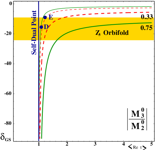
Figure 1: Ratio of unification scale gluino mass to wino mass as a function of Green-Schwarz coefficient $\delta_{\mathsc{gs}}$ and $\left\langle{\rm Re}\;t\right\rangle\geq 1$. Contours of $|M_{3}/M_{2}|$ at the boundary condition scale of $\Lambda_{\mathsc{uv}}=2\times 10^{16}~{}\mathrm{GeV}$ of 0.75 (solid green) and 0.33 (dashed red) are given. The upper set of contours have ${\rm sgn}(M_{3})=-{\rm sgn}(M_{2})$, while for the lower set of contours ${\rm sgn}(M_{3})={\rm sgn}(M_{2})$. The preferred region indicated by (39) for the $Z_{3}$ orbifold is shown by the shaded region. We have indicated the position of our two benchmark points D and E.

In (40) we see the essential elements for addressing the fine-tuning in the electroweak sector: A universal contribution from the Green-Schwarz counterterm and group-dependent contributions which distinguish the gauginos of the asymptotically free $SU(3)$ group from the others. The interplay between these contributions, without the anomaly contribution in (40), was studied in orbifold models in [50]. For the right combinations of relative phase between $F^{T}$ and $M$ (we have tacitly assumed zero relative phase) and sign of $G_{2}\left(t,\bar{t}\right)$ it is possible to diminish the gluino mass relative to the other gauginos. This is exhibited in Figure 1 where we have highlighted the region preferred by the $Z_{3}$ orbifold. Remarkably, it appears that the $Z_{3}$ orbifold, with moduli stabilized just slightly away from their self-dual points, actually prefers a light gluino.

To complete our model and generate spectra for use as benchmarks we need to exhibit the remainder of the soft supersymmetry breaking terms. The insistence on modular weights $n_{i}=-1$ generates a model similar to the no-scale models in which all soft terms are zero at the tree level, independent of the ultimate value of $\left\langle t\right\rangle$ provided $\left\langle F^{S}\right\rangle=0$. As a result, much of the one loop correction to the various soft terms will also vanish, as they are proportional to tree level soft supersymmetry breaking. The remainder of the one loop soft term contributions depend on the manner in which the theory is regulated. The complete set of one loop terms was computed in full generality in [12] and specialized to the cases we are considering here in [22]. We reserve further details for the Appendix. The full set of soft supersymmetry breaking terms we will employ are then

$$M_{a} = \frac{g_{a}^{2}\left(\mu\right)}{2}\left\{2\left[\frac{\delta_{\mathsc{gs}}}{16\pi^{2}}+b_{a}\right]G_{2}\left(t,\bar{t}\right)F^{T}+\frac{2}{3}b_{a}\overline{M}\right\}$$

$$A_{ijk} = m_{3/2}\left[\gamma_{i}+\gamma_{j}+\gamma_{k}\right]$$

$$m_{i}^{2} = \gamma_{i}m_{3/2}^{2}.$$ (43)

Let us note that the scalar masses in (43) are truly anomaly mediated, in the sense that their origin lies in the superconformal anomaly and they are proportional to the supergravity auxiliary field directly, though they are nonzero at one loop and positive for the matter fields (though potentially negative for the two Higgs fields of the MSSM, depending on the value of $\tan\beta$). This is in contrast to the masses found in [31, 32] and subsequent work, which are a special case of the more generalized anomaly-induced soft terms found in [12]. The case considered here differs from the “standard” AMSB in the assumptions made about the regularization of the theory. We refrain from designating this true “anomaly mediation” because the soft terms considered here are manifestly not insensitive to UV physics, as is the hallmark of the anomaly mediated supersymmetry breaking paradigm. But just as in the cases of anomaly mediation so often considered in the literature, these models will contain nearly-degenerate charginos and lightest neutralinos and have a typical supersymmetry breaking scale of $\mathcal{O}(10-20~{}\mathrm{TeV})$. Given the discussion in Section 2.2 we will define our second two benchmark points then as follows:

$${\rm Case\;D:}\qquad\left\{\tan\beta,\;m_{3/2},\;\delta_{\mathsc{gs}},\;\left\langle{\rm Re}\;t\right\rangle\right\} = \left\{45,\;20~{}\mathrm{TeV},\;-15,\;1.10\right\}$$ (44)

$${\rm Case\;E:}\qquad\left\{\tan\beta,\;m_{3/2},\delta_{\mathsc{gs}},\;\left\langle{\rm Re}\;t\right\rangle\right\} = \left\{30,\;20~{}\mathrm{TeV},\;-9,\;1.23\right\},$$ (45)

with the corresponding values of the soft terms to be given in Table 1 in Section 4 below. We choose to impose these boundary conditions at the scale $\Lambda_{\mathsc{uv}}=2\times 10^{16}~{}\mathrm{GeV}$ as in the previous section.

3 Partial gauge mediation

3.1 Theoretical motivation

Models of gauge mediation [51] are typically characterized by a scale at which supersymmetry breaking is transmitted to the observable sector that is far lower than the Planck or string scale. But this need not necessarily be the case. Of course if one wants the soft supersymmetry breaking terms to be dominated by the gauge-mediated contribution then one needs to suppress the relative gravity-mediated contribution which is always present. This can be accomplished simply by making the mass scale of the messenger particles much smaller than the string scale (the mass scale of the “messengers” in gravity-mediated models). The idea of gauge mediation drew its greatest motivation by the desire to have supersymmetry breaking communicated to the Standard Model at an energy scale far below any possible scale of flavor physics – hence the tendency to demand mass scales on the order of $100~{}\mathrm{TeV}$ for messenger fields and gravitino masses far below $1~{}\mathrm{GeV}$.

Here we will not try to address the problems of flavor that may be present in string-derived supergravity models, but merely address the possibility that gauge mediation of supersymmetry breaking from a hidden sector to the observable sector may well exist in addition to the standard gravity-mediated mechanism. In fact, given the generic occurrence of additional exotic vector-like pairs of matter charged under observable sector gauge groups in semi-realistic string compactifications [34, 52, 53, 54, 55] we can conclude that “partial” gauge mediation most certainly does occur in string-derived models. The only question is to whether or not these contributions to soft terms are comparable in size to those we described in the previous sections. In the approaches we will examine they are naturally comparable. The idea of combining gauge and gravity mediation is not new, particularly in the context of string theory [56, 57, 58, 59].

To review the basic elements of gauge mediation that we will need, let us begin with the messenger sector. We imagine a set of chiral fields $\Phi_{i}$ and $\overline{\Phi}_{i}$ that come in vector-like representations of one or more of the subgroups of the Standard Model. These fields experience a superpotential coupling to a chiral field $X$, which is a singlet under the gauge groups of the Standard Model, of

$$W=\lambda_{i}\overline{\Phi}_{i}X\Phi_{i}$$ (46)

so that should the chiral field $X$ receive a vacuum value $\left\langle X\right\rangle=M_{X}$ in its lowest component, we would have Dirac fermions with masses $\sim\lambda_{i}M_{X}$. Note that we have chosen a single field $X$ and diagonal couplings $\lambda_{ij}=\delta_{ij}\lambda_{i}$ in (46) for simplicity. The index $i$ can be thought of as counting the number of copies, or “flavors,” of each messenger field $\Phi$. The field $X$ is further assumed to carry the information of supersymmetry breaking through a nonzero highest component, so that $\left\langle X\right\rangle=M_{X}+\theta^{2}F^{X}$, and thus the messenger sector has mass splittings between its scalar and fermionic components of order $\sqrt{F^{X}}$.

When the messenger mass scale $M_{X}$ is lower than the GUT scale it is typical to employ messengers which form complete multiplets under a unified group such as $SU(5)$. This ensures that gauge coupling unification is preserved while providing a certain universality in the soft term expressions. From a string theory perspective it is preferable to relax this assumption, so we will instead invoke incomplete GUT multiplets as messengers [60], though we will continue to assume a universal mass splitting $F^{X}$ and adopt the simplification of a universal Yukawa coupling $\lambda_{i}=1$ in (46) and hence a universal messenger mass $M_{X}$. Each of the specific cases we will deal with below will be designed to ensure gauge coupling unification despite the incomplete GUT representations. It is of use to introduce the standard messenger index

$$N_{a}=\sum_{i=1}^{N_{F}}n_{a}^{i}$$ (47)

where $n_{a}^{i}$ is the Dynkin index for the representation $\mathbf{r}$ with flavor index $i$ under each Standard Model gauge group ${\cal G}_{a}$. It is normalized with a GUT normalization so that $n_{a}=1$ for a pair of $SU(N)$ fundamentals and $n_{1}=(6/5)Y^{2}$ for a messenger pair with hypercharge $Y$. While we adopt the $SU(5)$ GUT normalization on the hypercharges of our messenger fields so as to make contact with the standard cases in the literature, it is important to note that in realistic string constructions there is no reason to assume that vector-like messenger fields will have the same hypercharges as their Standard Model analogs [34, 61, 62, 63].

With these definitions, the gauge-mediated contributions to gaugino masses are given by

$$\delta M_{a}(\Lambda_{\mathsc{uv}})=\frac{g_{a}^{2}(\Lambda_{\mathsc{uv}})}{16\pi^{2}}N_{a}\frac{F^{X}}{M_{X}}$$ (48)

while those of the scalar masses are

$$\delta m_{A}^{2}(\Lambda_{\mathsc{uv}})=2\sum_{a}N_{a}C_{a}^{A}\left(\frac{g_{a}^{2}(\Lambda_{\mathsc{uv}})}{16\pi^{2}}\right)^{2}\left(\frac{F^{X}}{M_{X}}\right)^{2}$$ (49)

where $C_{a}^{A}$ is the standard quadratic Casimir for (SM) particle $\Phi^{A}$ with $C_{a}^{A}=(N^{2}-1)/2N$ for $SU(N)$ fundamentals and $(3/5)Y^{2}$ for hypercharge (properly normalized to GUT normalization). Since we imagine here only those cases for which $F^{X}\ll M_{X}^{2}$ we can dispense with all but the leading terms in the functions $f(x)$ and $g(x)$ of [51, 60]. We propose to add the contributions in (48) and (49) to those of the supergravity contributions described in the previous two sections. We should note that (48) and (49) were computed in the $\overline{DR}$ renormalization scheme appropriate to global supersymmetry [64] but here we wish to employ them in cases where the messenger masses will be much closer to the Planck scale, suggesting a regularization scheme appropriate to supergravity (such as Pauli-Villars) in called for. For the purposes of obtaining benchmark scenarios, however, we will ignore this technical, though potentially interesting, issue.

Standard analyses of gauge mediated supersymmetry breaking now would proceed by treating both $F^{X}$ and the messenger mass $M_{X}$ as free variables, with $F^{X}$ ultimately determined by some model-dependent mechanism which ensures $\left\langle W_{X}\right\rangle\neq 0$, since nonrenormalizable or Planck-suppressed operators are discarded. In the presence of supergravity the auxiliary field $F^{X}$ is determined by

$$F^{X}=-e^{K/2M_{\mathsc{pl}}^{2}}\left(\overline{W}_{\overline{X}}+\frac{X\overline{W}}{M_{\mathsc{pl}}^{2}}\right),$$ (50)

where we have restored the reduced Planck mass $M_{\mathsc{pl}}=2.4\times 10^{18}~{}\mathrm{GeV}$ for clarity. There is always a contribution, independent of any additional superpotential terms involving $X$, given by $F^{X}=-M_{X}m_{3/2}$ from the second term in (50). But in supergravity theories the mass splitting within the messenger sector is no longer given simply by $F_{X}$, which must be replaced in (48) and (49) by the off-diagonal mass terms of the complete supergravity potential.

For example in the minimal case $F^{X}=-M_{X}m_{3/2}$ (i.e. $\left\langle W_{X}\right\rangle\simeq 0$) then the messenger mass spectrum would be determined by (9)

$$V\big{|}_{\rm SUGRA}\ni|\tilde{\lambda}X|^{2}\left(|\Phi|^{2}+|\overline{\Phi}|^{2}\right)+m_{3/2}^{2}\left(|\Phi|^{2}+|\overline{\Phi}|^{2}\right)+\left(\tilde{\lambda}m_{3/2}M_{X}(M_{X}/M_{\mathsc{pl}})^{2}\Phi\overline{\Phi}+\mathrm{\;h.c.\;}\right),$$ (51)

where $\tilde{\lambda}=e^{K/2}\lambda$. Making the appropriate substitutions for $F_{X}$ in (48) and (49) we can see that the gauge-mediated contributions to soft terms in this case are proportional to the gravitino mass with a typical size

$$m_{\rm soft}\sim m_{3/2}\frac{1}{16\pi^{2}}\left(\frac{M_{X}}{M_{\mathsc{pl}}}\right)^{2}.$$ (52)

Even when tree level gravity-mediated soft terms are absent or suppressed, as in Sections 1 and 2, such gauge-mediated contributions would prove irrelevant unless the messenger mass $M_{X}$ was extremely close to the Planck scale.

We are thus led to consider cases in which supersymmetry continues to be broken in the hidden sector by one of the string moduli $S$ or $T$, generating an F-term of general magnitude $<F^{0}>\;\simeq\sqrt{3}m_{3/2}M_{\mathsc{pl}}$ to bring about a vanishing vacuum energy and generating a gravitino mass on the order of $1~{}\mathrm{TeV}$. In addition we will allow for some undetermined mechanism to generate a non-vanishing $\left\langle F_{X}\right\rangle$ through the first term in (50) as in typical gauge-mediated models. We will parameterize the size of this additional source of supersymmetry breaking through the parameter $k=F^{X}/F^{0}$, with $F^{0}$ identified with either $F^{S}$ or $F^{T}$ as in the previous sections.

3.2 A concrete realization

One of the reasons that gauge mediation is not often considered in the context of string theory is the difficulty in finding suitable messenger sectors when only renormalizable couplings are allowed. The fields need to be vector-like, charged under one or more of the subgroups of the Standard Model, remain light down to very low energies and be capable of communicating directly with the supersymmetry breaking of the hidden sector through operators that are not suppressed by powers of the Planck mass. Such circumstances are rare in actual string compactifications. However any massive vector-like pairs, charged under a subgroup of the Standard Model, can and will participate in gauge-mediation of supersymmetry breaking at least through the supergravity-generated second term in (50). Since all realistic string constructions contain such exotic vector-like states we can assert that “partial” gauge-mediation is a generic outcome of string theory that should not be neglected.

These potential messenger sectors tend to come in incomplete multiplets of $SU(5)$, however, instead of the $\mathbf{5}$ and $\overline{\mathbf{5}}$’s that are so commonly employed. What’s more, these models also predict an anomalous $U(1)$ whose breaking occurs at a scale $\Lambda_{X}\sim 10^{16}-10^{17}~{}\mathrm{GeV}$. If the singlet field $X$ were charged under this anomalous $U(1)$, as is typical, then we might expect the messenger mass $\left\langle X\right\rangle\simeq M_{X}$ to be of this magnitude as well, providing a concrete realization of the above scenario. Note that by assuming the messenger mass scale to be at or near the GUT scale we will preserve the apparent unification of gauge couplings in the MSSM up to small corrections.

In the context of Section 3.1 we will allow $\left\langle F^{X}\right\rangle$ to be a free parameter due to some $\left\langle W_{X}\right\rangle\neq 0$. Now the gauge-mediated contributions can be as large or larger than the tree-level supergravity contribution, depending on the relative size of the messenger mass, so we will return to the simplicity of the dilaton-dominated scenario of Section 1. Taking the tree level Kähler potential for the dilaton (no nonperturbative corrections so $a_{\rm np}=1$) and

$$\left\langle F^{0}\right\rangle=\left\langle F^{S}\right\rangle=\frac{2}{g_{\mathsc{str}}^{2}}\sqrt{3}m_{3/2}M_{\mathsc{pl}}$$ (53)

then we can employ (48) and (49) with $\left\langle F^{X}\right\rangle=k\left\langle F^{S}\right\rangle$. Note that the gravity and gauge-mediated contributions are competitive whenever

$$\frac{k}{16\pi^{2}}\frac{M_{\mathsc{pl}}}{M_{X}}\simeq 1.$$ (54)

It is interesting to note that this equality is satisfied for $k\simeq 1$ when the messenger mass is near the anomalous $U(1)_{X}$ scale.

For our messenger sector we will introduce $n_{D}$ pairs of messengers which are triplets under $SU(3)$ and $n_{L}$ pairs of messengers which are doublets under $SU(2)_{L}$. We will not introduce any specific messengers which carry only Standard Model hypercharge. In fact, we leave the hypercharge assignments of the messenger fields a free variable and work only with the overall messenger index $N_{1}=\sum_{i}n_{i}^{i}$ which we treat as a continuous free parameter. If our messenger fields happen to have the hypercharge of their Standard Model analogs, then $N_{1}=(1/5)(2n_{D}+3n_{L})$. We follow the standard practice of setting the initial scale for our soft parameters at the messenger mass scale $M_{X}$, leaving the free variables that define our models as $\left\{\tan\beta,\;m_{3/2},\;M_{X},\;k,\;n_{D},\;n_{L},\;N_{1}\right\}$.

3.3 Soft terms and benchmark choices

We seek cases where the gauge-mediated masses are of the same order of magnitude as the gravitino mass, so we return to the case with $\left\langle F^{T}\right\rangle=0$ and $\left\langle F^{S}\right\rangle\neq 0$ with $a_{\rm np}=1$. Since we will only consider cases where $M_{X}\simeq M_{\mathsc{str}}$ let us take $g_{1}(M_{X})\simeq g_{2}(M_{X})\simeq g_{3}(M_{X})\simeq g_{\mathsc{str}}$ so that the complete, properly normalized, gaugino masses are given by

$$M_{3} = \sqrt{3}m_{3/2}\left[1+n_{D}\frac{k}{8\pi^{2}}\frac{M_{\mathsc{pl}}}{M_{X}}\right]$$

$$M_{2} = \sqrt{3}m_{3/2}\left[1+n_{L}\frac{k}{8\pi^{2}}\frac{M_{\mathsc{pl}}}{M_{X}}\right]$$

$$M_{1} = \sqrt{3}m_{3/2}\left[1+N_{1}\frac{k}{8\pi^{2}}\frac{M_{\mathsc{pl}}}{M_{X}}\right]$$ (55)

and the remaining soft terms are

$$m_{Q}^{2} = m_{3/2}^{2}\left[1+6\left(\frac{4}{3}n_{D}+\frac{3}{4}n_{L}+\frac{1}{60}N_{1}\right)\frac{k^{2}}{(8\pi^{2})^{2}}\left(\frac{M_{\mathsc{pl}}}{M_{X}}\right)^{2}\right]$$

$$m_{U}^{2} = m_{3/2}^{2}\left[1+6\left(\frac{4}{3}n_{D}+\frac{4}{15}N_{1}\right)\frac{k^{2}}{(8\pi^{2})^{2}}\left(\frac{M_{\mathsc{pl}}}{M_{X}}\right)^{2}\right]$$

$$m_{D}^{2} = m_{3/2}^{2}\left[1+6\left(\frac{4}{3}n_{D}+\frac{1}{15}N_{1}\right)\frac{k^{2}}{(8\pi^{2})^{2}}\left(\frac{M_{\mathsc{pl}}}{M_{X}}\right)^{2}\right]$$

$$m_{L}^{2} = m_{3/2}^{2}\left[1+6\left(\frac{3}{4}n_{L}+\frac{3}{20}N_{1}\right)\frac{k^{2}}{(8\pi^{2})^{2}}\left(\frac{M_{\mathsc{pl}}}{M_{X}}\right)^{2}\right]$$

$$m_{E}^{2} = m_{3/2}^{2}\left[1+\frac{18}{5}N_{1}\frac{k^{2}}{(8\pi^{2})^{2}}\left(\frac{M_{\mathsc{pl}}}{M_{X}}\right)^{2}\right].$$ (56)

with $m_{H_{u}}^{2}=m_{H_{D}}^{2}=m_{L}^{2}$ and $A=\sqrt{3}m_{3/2}$. We have again chosen a positive relative sign between the contributions to gaugino masses in (55) from gauge messengers and those arising from supergravity.

The choice of messenger indices is dictated by the need to obtain sufficiently large radiative corrections to the lightest CP-even Higgs mass. By introducing messengers charged solely under $SU(3)$ a heavy gluino is produced that can achieve the necessary Higgs mass with light scalars. Such a scenario was considered in the context of low-energy gauge mediation in the context of string theory in [58]. When Standard Model-like hypercharge assignments for these messengers are assumed the bino mass $M_{1}$ tends to be much larger than the wino mass $M_{2}$ at the initial high-energy input scale, producing a gaugino sector similar to that of anomaly-mediation. We have therefore chosen to allow non-standard hypercharges for the messenger fields and have selected a value for $N_{1}$ that gives gaugino mass in the gravity-mediated regime. We take the messenger mass scale to be intermediate between the GUT scale and the Planck scale: $\Lambda_{\mathsc{uv}}=M_{X}=8\times 10^{16}~{}\mathrm{GeV}$, which was a typical anomalous $U(1)$ scale in those models that gave rise to suitable messenger fields [33]. Our two benchmarks points for this section are then given by the following parameter sets

$${\rm Case\;F:}\qquad\left\{\tan\beta,\;m_{3/2},\;n_{D},\;n_{L},\;N_{1}\right\}=\left\{10,\;120~{}\mathrm{GeV},\;4,\;0,\;(3/5)\right\}$$ (58)

$${\rm Case\;G:}\qquad\left\{\tan\beta,\;m_{3/2},\;n_{D},\;n_{L},\;N_{1}\right\}=\left\{20,\;130~{}\mathrm{GeV},\;3,\;0,\;(3/5)\right\}$$ (59)

with $k=1$. Note that both of these examples are close in spirit to the standard gauge-mediated examples in that the gravitino, while not the LSP, is much lighter than the supergravity-dominated models of our previous cases.

4 Collected spectra and signatures

4.1 Benchmark spectra and phenomenology

Point	A	B	C	D	E	F	G
$\tan\beta$	10	5	5	45	30	10	20
$\Lambda_{\mathsc{uv}}$	$2\times 10^{16}$	$2\times 10^{16}$	$2\times 10^{16}$	$2\times 10^{16}$	$2\times 10^{16}$	$8\times 10^{16}$	$8\times 10^{16}$
$M_{1}$	198.7	220.1	215.3	606.5	710.8	278.9	302.2
$M_{2}$	172.1	162.3	137.3	195.2	244.6	213.4	231.2
$M_{3}$	154.6	122.3	82.4	-99.2	-89.0	525.4	482.9
$A_{t}$	193.0	204.8	195.4	286.0	352.5	210.7	228.2
$A_{b}$	205.3	235.3	236.3	390.6	501.5	211.6	229.2
$A_{\tau}$	188.4	200.0	188.9	158.1	272.5	210.3	227.8
$m_{Q_{3}}^{2}$	$(1507)^{2}$	$(3216)^{2}$	$(4323)^{2}$	$(2035)^{2}$	$(2144)^{2}$	$(286)^{2}$	$(276)^{2}$
$m_{U_{3}}^{2}$	$(1504)^{2}$	$(3209)^{2}$	$(4312)^{2}$	$(1487)^{2}$	$(1601)^{2}$	$(290)^{2}$	$(281)^{2}$
$m_{D_{3}}^{2}$	$(1505)^{2}$	$(3213)^{2}$	$(4319)^{2}$	$(1713)^{2}$	$(1870)^{2}$	$(287)^{2}$	$(277)^{2}$
$m_{L_{3}}^{2}$	$(1503)^{2}$	$(3208)^{2}$	$(4312)^{2}$	$(1361)^{2}$	$(1489)^{2}$	$(125)^{2}$	$(135)^{2}$
$m_{E_{3}}^{2}$	$(1502)^{2}$	$(3206)^{2}$	$(4308)^{2}$	$(756)^{2}$	$(1139)^{2}$	$(140)^{2}$	$(152)^{2}$
$m_{Q_{1,2}}^{2}$	$(1508)^{2}$	$(3220)^{2}$	$(4328)^{2}$	$(2347)^{2}$	$(2347)^{2}$	$(286)^{2}$	$(276)^{2}$
$m_{U_{1,2}}^{2}$	$(1506)^{2}$	$(3215)^{2}$	$(4321)^{2}$	$(2050)^{2}$	$(2050)^{2}$	$(290)^{2}$	$(281)^{2}$
$m_{D_{1,2}}^{2}$	$(1505)^{2}$	$(3213)^{2}$	$(4319)^{2}$	$(1919)^{2}$	$(1919)^{2}$	$(287)^{2}$	$(277)^{2}$
$m_{L_{1,2}}^{2}$	$(1503)^{2}$	$(3208)^{2}$	$(4312)^{2}$	$(1533)^{2}$	$(1533)^{2}$	$(125)^{2}$	$(135)^{2}$
$m_{E_{1,2}}^{2}$	$(1502)^{2}$	$(3206)^{2}$	$(4308)^{2}$	$(1252)^{2}$	$(1252)^{2}$	$(140)^{2}$	$(152)^{2}$
$m_{H_{u}}^{2}$	$(1500)^{2}$	$(3199)^{2}$	$(4298)^{2}$	$-(797)^{2}$	$-(331)^{2}$	$(125)^{2}$	$(135)^{2}$
$m_{H_{d}}^{2}$	$(1503)^{2}$	$(3208)^{2}$	$(4312)^{2}$	$(858)^{2}$	$(1392)^{2}$	$(125)^{2}$	$(135)^{2}$

Table 1: Soft Term Inputs. Initial values of supersymmetry breaking soft terms in GeV, including the full one-loop contributions, at the initial scale given by $\Lambda_{\mathsc{uv}}$. All points are taken to have $\mu>0$. The actual value of $\tan\beta$ is fixed in the EWSB conditions. See the text for further discussion of the parameters and their origins. Ways to convert these points into model lines are discussed at the end of the Appendix.

The seven benchmark scenarios described in Sections 1 through 3 give rise to seven sets of high energy input values for renormalization group (RG) evolution to the electroweak scale. These values are determined by substituting the specified parameters into the complete one-loop expressions for soft terms given in the Appendix. The numerical value of these input quantities are summarized in Table 1. Actual evolution of these parameters was carried out using the publicly-available code SuSpect [66] which performs RG integration at the two-loop level from the specified input scale to the scale $M_{z}$.

SuSpect uses the following quantities as inputs:

$$\alpha_{\mathsc{em}}^{\overline{MS}}(M_{Z})=1/127.938,\qquad\alpha_{s}^{\overline{MS}}(M_{Z})=0.118,\qquad\bar{s}^{2}_{W}=0.23117,$$ (60)

as well as the following pole masses for heavy SM fermions:

$$M_{t}=174.3~{}\mathrm{GeV},\qquad M_{b}=4.62~{}\mathrm{GeV},\qquad M_{\tau}=1.778~{}\mathrm{GeV}.$$ (61)

Determination of parameters in the Higgs sector (such as the value of the $\mu$ parameter inferred from EWSB) are computed at a scale given by the geometric mean of the two stop masses. We have chosen the number of iterations to achieve consistency in the EW sector to be five. The light CP-even Higgs mass is calculated by using the full one-loop tadpole method and includes leading NLO QCD corrections as implemented in Subhpole [67]. The values of $m_{h}$ determined by SuSpect for the benchmark scenarios have been checked against FeynHiggs [68] and found to be in acceptable agreement. The radiative correction at NLO to all sparticles masses are included and can be significant for many mass eigenstates, particularly in the gaugino sector, affecting some production rates and branching ratios noticeably. The resulting low-energy spectrum for the seven benchmark models is summarized in Table 2.

Point	A	B	C	D	E	F	G
$\tan\beta$	10	5	5	45	30	10	20
$\Lambda_{\mathsc{uv}}$	$2\times 10^{16}$	$2\times 10^{16}$	$2\times 10^{16}$	$2\times 10^{16}$	$2\times 10^{16}$	$8\times 10^{16}$	$8\times 10^{16}$
$m_{3/2}$	1500	3200	4300	20000	20000	120	130
$M_{1}$	84.0	95.6	94.7	264.7	309.9	106.2	115.7
$M_{2}$	133.7	127.9	108.9	159.0	198.5	154.6	169.6
$M_{3}$	346.5	264.0	175.6	-227.5	-203.9	1201	1109
$m_{\widetilde{N}_{1}}$	77.9	93.1	90.6	171.6	213.0	103.5	113.1
$m_{\widetilde{N}_{2}}$	122.3	132.2	110.0	264.8	309.7	157.6	173.1
$m_{\widetilde{C}_{1}^{\pm}}$	119.8	131.9	109.8	171.6	213.0	157.5	173.0
$m_{\tilde{g}}$	471	427	329	351	326	1252	1158
$\widetilde{B}\;\%|_{\rm LSP}$	89.8 %	98.7 %	93.4 %	0 %	0 %	99.4 %	99.4 %
$\widetilde{W}_{3}\%|_{\rm LSP}$	2.5 %	0.6 %	4.6 %	99.7 %	99.7 %	0.1 %	0.06 %
$m_{h}$	114.3	114.5	116.4	114.7	114.9	115.2	115.5
$m_{A}$	1507	3318	4400	887	1792	721	640
$m_{H}$	1510	3329	4417	916	1821	722	644
$\mu$	245	631	481	1565	1542	703	643
$m_{\tilde{t}_{1}}$	947	1909	2570	1066	1105	954	886
$m_{\tilde{t}_{2}}$	1281	2639	3530	1678	1897	1123	991
$m_{\tilde{c}_{1}}$, $m_{\tilde{u}_{1}}$	1553	3254	4364	2085	2086	1127	1047
$m_{\tilde{c}_{2}}$, $m_{\tilde{u}_{2}}$	1557	3260	4371	2382	2382	1132	1054
$m_{\tilde{b}_{1}}$	1282	2681	3614	1213	1714	1053	971
$m_{\tilde{b}_{2}}$	1540	3245	4353	1719	1921	1123	1037
$m_{\tilde{s}_{1}}$, $m_{\tilde{d}_{1}}$	1552	3252	4362	1950	1948	1126	1045
$m_{\tilde{s}_{2}}$, $m_{\tilde{d}_{2}}$	1560	3261	4372	2383	2384	1135	1057
$m_{\tilde{\tau}_{1}}$	1491	3199	4298	559	1038	153	135
$m_{\tilde{\tau}_{2}}$	1502	3207	4308	1321	1457	221	252
$m_{\tilde{\mu}_{1}}$, $m_{\tilde{e}_{1}}$	1505	3207	4309	1274	1282	182	196
$m_{\tilde{\mu}_{2}}$, $m_{\tilde{e}_{2}}$	1509	3211	4313	1544	1548	200	217
$m_{\tilde{\nu_{3}}}$	1500	3206	4307	1314	1453	183	198

Table 2: Sample Spectra. All masses are in GeV. For the purposes of calibrating these results with those of other software packages we also provide the running gaugino masses at the scale $M_{Z}$, which include NLO corrections. See the text for further discussion of the parameters and their origins. Ways to convert these points into model lines are discussed at the end of the Appendix.

The benchmark models we present are quite interesting phenomenologically, and should be studied in some detail. They present challenges for present and future colliders that are rather different from previously studied models. Here we will only draw attention to a few general features.

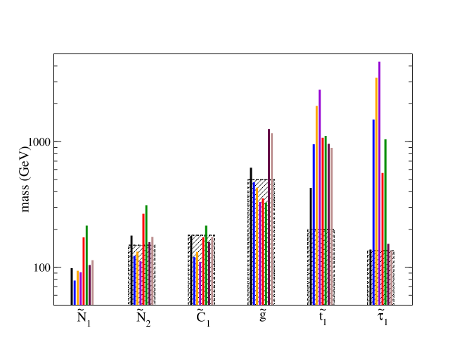
Figure 2: Sparticle masses for different benchmark models. For each superpartner, lines from left to right correspond to mSUGRA Point B of [1], and our benchmark models A through G. The mass of the particle is represented by the height of the line. Gray bars are crude estimates of Tevatron reaches, i.e. any superpartner in the gray region could be observed at the Tevatron. That reach of course depends on backgrounds which will vary depending on the details of the signal, so the gray regions are just approximate guides for the non-expert reader. We have not studied the detectability of these models at the LHC.

Figure 2 shows a summary of a number of the superpartner masses, along with crude estimates of Tevatron reaches. For comparison we also include the Snowmass benchmark point most favorable for observation at the Tevatron [1]. In general the benchmark models we study have gauginos observable at the Tevatron, as expected for supersymmetric worlds in which electroweak symmetry breaking is explained by supersymmetry without excessive fine tuning [3].

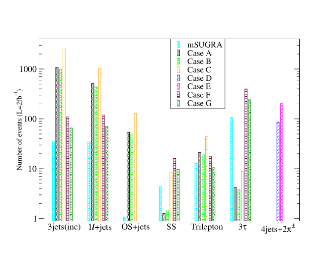
Figure 3: Number of superpartner events of different signatures for different models at the Tevatron with $2\mbox{fb}^{-1}$. These numbers are based on counting topologies from Pythia at the parton level with no kinematic or geometric cuts. Every signature has missing energy. From left to right, the signatures are: (1) inclusive multi-jets $n_{jets}\geq 3$, (2) one lepton plus $n_{jets}\geq 2$, (3) opposite sign dileptons plus $n_{jets}\geq 2$, (4) same-sign dileptons, (5) trilepton, (6) 3 taus plus jets [before decaying the taus], and (7) 4 jets plus 2 soft, isolated, high impact parameter charged pions [some pions are like–signed]. For signatures (4)-(6), no requirement is made on the number of jets. A background analysis must of course be done to be sure any given channel is detectable, but models with hundreds of events are presumably detectable for the first two signatures, and models with tens of events for the rest. The same-sign dilepton channel has smaller backgrounds: even a handful of clean events may constitute a signal. Here the model labeled “mSUGRA” is the cMSSM Point B of [1].

Figure 3 shows naive estimates of numbers of events in 2 fb^-1 integrated luminosity for various models and various inclusive signatures. The signature of these models are calculated using PYTHIA [69], but only at the generator level: no geometric or kinematic cuts or triggering efficiencies are applied, no jet clustering is performed, tau leptons are not decayed, etc. The event numbers are only meant to illustrate the generic features of each model and demonstrate the experimental challenges. In general, there will be too few events from any single exclusive process to isolate it by cuts and observe a clean signal, but significant excesses could be established in several inclusive signatures. In all these cases there are of course backgrounds, but typically the backgrounds are not so large as to prevent the experiments from establishing an excess. Note that each model has a different pattern, and it could be possible to learn quite a bit about the underlying physics from the relative sizes of different inclusive signals, as illustrated in Figure 4. Despite the fact that the event numbers are based on unsophisticated estimates, the resulting correlations are quite distinct and should be robust under more detailed analyses. Once a signal of beyond the Standard Model physics is established it will be an exciting challenge to determine which superpartners are being produced, their masses and branching ratios, and their implications for the underlying theory.

Some specific features and signatures are worth noting. First, the negative gluino mass of the two moduli-dominated models D and E is physical and observable [70]. Next for these models the LSP is predominantly a wino that is almost degenerate with the lightest chargino so that the dominant decay mode of the chargino is $\tilde{W}^{\pm}\to\tilde{W}^{0}\pi^{\pm}$ [14]. This is quite similar to the anomaly-mediated supersymmetry breaking models, but in AMSB the ratio of gaugino masses $M_{1}:M_{2}:|M_{3}|$ is approximately $2.8:1:7.1$ so that the gluino is very heavy and out of reach for the Tevatron. Thus in the usual anomaly-mediated cases the chargino pair can only be produced directly and not from gluino decay. In our cases D and E, however, gluino masses are $351~{}\mathrm{GeV}$ and $325~{}\mathrm{GeV}$, respectively, so the cross section for gluino pair production is quite large. The gluino has the decay mode $\tilde{g}\to\tilde{W}^{\pm}qq^{\prime}$ with a branching ratio about 50%, followed by $\tilde{W}^{\pm}\to\tilde{W}^{0}\pi^{\pm}$. Thus there will be large missing transverse energy with four jets plus two soft, high impact parameter pions. Since the chargino $\tilde{W}^{\pm}$ emerges from gluino decay it is quite energetic so the pion will also be reasonably energetic and give a good signature to detect these models. Furthermore, gluino production will lead to pairs of like–signed pions in these events. The number of such events expected in cases D and E are shown in the last set of columns in Figure 2. These are interesting new collider signatures for the Tevatron, and for AMSB at the LHC, that to our knowledge have not been studied previously.

For models F and G the stau $\tilde{\tau}_{1}$ is lighter than $\tilde{N}_{2}$ and $\tilde{C}_{1}$, so $\widetilde{N_{2}}\rightarrow\tilde{\tau}\tau$ and $\widetilde{C_{1}}\rightarrow\tilde{\tau}\nu_{\tau}$ dominates, leading to a large three tau signal and reducing the trilepton rate. Although model C also has many trilepton events, the reason is different. For model C, the $\tilde{N}_{2}\tilde{C}_{1}$ cross section is quite large, but the leptonic branching ratios of $\tilde{N}_{2}$ and $\tilde{C}_{1}$ are smaller. Model C has jets plus missing energy signatures while models F and G do not.

Detecting and studying these models presents interesting challenges for experiments at the LHC, which, in principle, has the kinematic reach to produce all superpartners. However, many of the scalars are quite heavy, and will have small production rates. The models with light gluinos have relatively little missing transverse energy and large backgrounds. Models F and G have heavier gluinos with mainly two–body decays dominated by $\tilde{g}\to\tilde{b}\bar{b},\;\tilde{t}\bar{t}$. All of our models have at least some superpartners that will be detected at a $500~{}\mathrm{GeV}$ linear collider. With a $520~{}\mathrm{GeV}$ linear collider every model allows the study of several superpartners, though clearly not all.

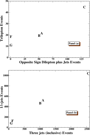
Figure 4: Correlations between the number of events in different signatures for $2\mbox{fb}^{-1}$. Cases C, FG, and AB are well separated from each other. By comparing several such signatures, many models can be identified at the Tevatron alone. A and B are difficult to separate at the Tevatron but since their $\mu$, squark and slepton masses are different, they should have different predictions for low energy experiments (e.g. in rare decays or $g_{\mu}-2$) and for LHC. Case G can be distinguished from others by the 3$\tau$ signature. Cases D and E (not shown here) have their unique 4 jets plus 2 isolated soft, high impact parameter pions signature with quite different event rates.

Further discrimination between models can be obtained by studying ratios of numbers of events of different types of signatures. An example of this is displayed in Figure 4 where two different pairs of signatures from Figure 3 are analyzed. By comparing several such signatures the underlying physics of many models can be identified at the Tevatron alone. While cases A and B are difficult to separate at the Tevatron, it may be possible to distinguish between them by their different predictions for low energy experiments or by their different predictions for scalar masses accessible at the LHC. Case G can be distinguished from the others by the 3$\tau$ signature. Case D and E have their unique 4 jets plus 2 isolated soft, high impact parameter pions signature with quite different event rates (86 and 201 respectively), so that they can be easily distinguished from other cases and amongst themselves.

We have checked that all of our benchmark models are not inconsistent with indirect constraints on superpartner masses. For example, the SUSY contribution to the muon anomalous magnetic moment for all models falls within the “conservative” bound obtained in [71], particularly if one favors the Standard Model prediction based on tau decay data. If one prefers instead the Standard Model prediction based on $e^{+}e^{-}$ collider data then all models can be made consistent with measurements at the the $2\sigma$ level by simply increasing the value of $\tan\beta$. As our focus has been on studying collider signatures for a range of $\tan\beta$ values we have chosen not to tune our values in this manner. The same is true for ${\rm Br}(b\to s\gamma)$ in these models.

The thermal relic density of LSP neutralinos was computed for all of these models using the DarkSUSY program [72]. In general, the $\Omega_{\rm LSP}{\rm h}^{2}$ results are very sensitive to some parameters so we view any values below $\Omega_{\rm LSP}{\rm h}^{2}\sim 2$ as satisfactory for the purposes of a benchmark model. For example, in model A the relic density as computed by DarkSUSY is $\Omega_{\rm LSP}{\rm h}^{2}=1.9$. However, lowering the top quark mass to $173.0~{}\mathrm{GeV}$ reduces this number to $\Omega_{\rm LSP}{\rm h}^{2}=0.14$. Alternatively, increasing the value of $\tan\beta$ from 10 to 12 changes this number to $\Omega_{\rm LSP}{\rm h}^{2}=1.07$. For both of the small modifications described above the superpartner spectrum – and thus, the collider signature of this model – is largely unchanged. The sensitivity of the relic density in this model (and model B, the only other case where the LSP relic density was larger than the cosmologically preferred region), is due to the importance of chargino/neutralino coannihilations for these models [73]. Our focus in this work is not to impose aggressive constraints on the MSSM parameter space but rather to study the collider signatures of a representative sample of theory-motivated models, so we have chosen not to adjust our input parameters in such an artificial way. Consistency with all indirect constraints on superpartners can be obtained by small corrections to our benchmark points along any of the indicated “model lines” suggested in the Appendix.

4.2 Fine Tuning

Any discussion of fine-tuning must necessarily involve certain subjective statements. One commonly employed tool for comparing models in a semi-quantitative way is the “sensitivity parameter” of Barbieri and Giudice [74] which measures the relative change in the Z-mass when a high-scale input parameter is varied. However, we believe that the degree of fine-tuning in a given model may be more profitably thought of as divided between an element that involves cancellations among various terms from the soft supersymmetry breaking Lagrangian, and an element that involves a measure of sensitivity arising from the overall scale of supersymmetry breaking relative to the Z-mass scale. As was pointed out some time ago [75] it is really the former that is a measure of the fine-tuning in a given theory, while the latter may often give misleading measures of tuning – particularly when the entire parameter space of a particular model implies a consistently high supersymmetry breaking scale as characterized by the gravitino mass or scalar/gaugino masses. The mere existence of a large scale in the theory need not necessarily imply large fine-tuning, as was demonstrated for example in [76], but the cancellation of large numbers against one another to produce a much smaller number almost certainly does if such cancellations can not be explained from the underlying theory.

The degree of cancellation that a particular model of supersymmetry breaking requires to obtain the correct Z-boson mass can be expressed by simply expanding the formula that determines $M_{Z}$ at the electroweak scale

$$\frac{M_{Z}^{2}}{2}=-\mu^{2}(t)+\left(\frac{m^{2}_{H_{D}}(t)-m^{2}_{H_{U}}(t)\tan^{2}\beta}{\tan^{2}\beta-1}\right),$$ (62)

with $t=\ln(\Lambda_{\mathsc{uv}}/Q)$, in terms of semi-analytic solutions for the running parameters in terms of the input parameters at the high scale $\Lambda_{\mathsc{uv}}$ and a given value of $\tan\beta$ [77]. For example, taking $\Lambda_{\mathsc{uv}}=\Lambda_{\mathsc{gut}}=2\times 10^{16}~{}\mathrm{GeV}$, the result for $m_{\rm top}(M_{Z})=170$ and $\tan\beta=30$ is

$$M_{Z}^{2} = -1.5\mu^{2}(\mathsc{uv})+6.4M_{3}^{2}(\mathsc{uv})-0.4M_{2}^{2}(\mathsc{uv})+0.0003M_{1}^{2}(\mathsc{uv})-1.2m^{2}_{H_{U}}(\mathsc{uv})$$ (63)

$$-0.08m^{2}_{H_{D}}(\mathsc{uv})+0.8m^{2}_{Q_{3}}(\mathsc{uv})+0.7m^{2}_{U_{3}}(\mathsc{uv})+0.03(m^{2}_{D_{3}}(\mathsc{uv})+m^{2}_{L_{3}}(\mathsc{uv})+m^{2}_{E_{3}}(\mathsc{uv}))$$

$$+0.2A_{t}^{2}(\mathsc{uv})-0.6A_{t}(\mathsc{uv})M_{3}(\mathsc{uv})-0.1A_{t}(\mathsc{uv})M_{2}(\mathsc{uv})-0.002A_{t}(\mathsc{uv})M_{1}(\mathsc{uv})$$

$$+0.5M_{2}(\mathsc{uv})M_{3}(\mathsc{uv})+0.06M_{1}(\mathsc{uv})M_{3}(\mathsc{uv})+0.01M_{1}(\mathsc{uv})M_{2}(\mathsc{uv}).$$

If the smallness of $M_{Z}=91.187~{}\mathrm{GeV}$ is not to be the result of a miraculous cancellation between large numbers then at least one of the following must occur: either certain relations among the soft terms and $\mu$ parameter must exist that guarantee cancellations over a wide range of parameters, or each of the individual terms in (63) must be no more than a few times $M_{Z}$ in size. The first could occur in theories of supersymmetry breaking. Even the cMSSM predicts certain “relations” among soft terms that are postulated to hold over all parameters: namely that gaugino masses and scalar masses are unified. But in [3] it was argued that this alone is not sufficient to prevent fine-tuning in the EWSB sector without also postulating a robust relationship between $\mu$ and $M_{3}$ (the two most crucial parameters in determining the Z boson mass). The conclusion drawn there was that the only reasonable way to avoid unnatural cancellations in the determination of $M_{Z}$ is for both $\mu$ and $M_{3}$ to individually be small. This implies that a certain degree of nonuniversality in the gaugino masses is beneficial in reducing EWSB fine-tuning while satisfying the search limits from LEP. Note that the scalar masses in (63) are far less important in this regard.

For a given model we can determine everything in (63), apart from $\mu(\mathsc{uv})$ itself, which has nothing to do a priori with supersymmetry breaking, as a function of the value of the coupling constant at the string scale $g_{\mathsc{str}}^{2}$ (which we can take to be $g_{\mathsc{str}}^{2}\simeq 1/2$), the gravitino mass, and a small number of free parameters related to the given model. Let us take as an example the class of models from Section 2. After choosing the initial scale and the value of $\tan\beta$ the only free parameters are $m_{3/2}$, $\delta_{\mathsc{gs}}$ and $\left\langle{\rm Re}\;T\right\rangle$. Substituting (43) into (63) with $\delta_{\mathsc{gs}}=-9$ and factoring out the gravitino mass gives

$$\left(\frac{M_{Z}}{100~{}\mathrm{GeV}}\frac{1~{}\mathrm{TeV}}{m_{3/2}}\right)^{2}=-1.5\left(\frac{\mu(\mathsc{uv})}{100~{}\mathrm{GeV}}\frac{1~{}\mathrm{TeV}}{m_{3/2}}\right)^{2}+0.1+0.7(t+\bar{t})G_{2}\left(t,\bar{t}\right)+1.2(t+\bar{t})^{2}G_{2}^{2}(t,\bar{t}).$$ (64)

The first constant is the contribution of the scalar masses in (63) with some addition from the anomaly-generated loop corrections to the gaugino masses. The case for other values of $\delta_{\mathsc{gs}}$ is quite similar. The fine-tuning arising from cancellations in the soft supersymmetry breaking Lagrangian is clearly controlled by the value of $\left\langle{\rm Re}\;T\right\rangle$ through the combination $(t+\bar{t})G_{2}\left(t,\bar{t}\right)$. For values of $\left\langle{\rm Re}\;T\right\rangle$ just larger than its self-dual point this combination is negative and less than unity, thus providing a model that has a very low degree of internal cancellation.

But of course this is only part of the story. The fact that all parameters in (64) are $\mathcal{O}(1)$ and roughly the same size implies that no large cancellation is required in this model to achieve the correct Z-mass provided the gravitino mass (scale) is approximately 1 TeV. But since all soft supersymmetry breaking terms are induced at the loop level, we expect $m_{3/2}\sim 16\pi^{2}M_{z}\sim 15~{}\mathrm{TeV}$. The need for such a large scale in the theory is quite clear: the LEP limit on the Higgs mass of $m_{h}\geq 114~{}\mathrm{GeV}$ implies, at least to a first approximation, that some squark masses must be large in order to generate large radiative corrections to the Higgs mass that are only logarithmically sensitive to scale. This can be achieved when the entire scalar sector of the theory is heavy at the high energy scale, or alternatively the scalar masses can start small at the high scale and the necessary large squark masses can be induced through RG evolution by a large gluino mass.

Thus some degree of tuning arising from the overall scale will likely be present in many low-energy models of supersymmetry breaking, but those with large gluino masses also give rise to troubling cancellations. Issues of tuning in the scale of soft terms are intimately related to the question of generating the supersymmetric $\mu$ parameter and are beyond the scope of this paper. We have not found models with small tunings associated with the overall scale, though we look at a significant class of string effective theories. Here we have chosen instead to be guided by [3] and have sought models that are capable of generating a sufficiently massive Higgs boson without introducing large internal cancellations within the soft supersymmetry breaking Lagrangian itself. Each of our models involves robust relations among the soft terms in the theory, in a manner dictated by the fundamental theory as in (64), which reduces the cancellations required in the soft supersymmetry-breaking sector relative to the typically-studied universal models. In this limited sense, then, we find these models to be more “natural” than their universal counterparts, though some degree of tuning remains.

Conclusion

In many ways effective field theories derived from strings are at once more constrained and also richer in their phenomenology than the universal scenario of minimal supergravity upon which so many previous benchmark cases are based. They are richer in that patterns of nonuniversality, particularly in the gaugino mass sector, are quite common; they are more constrained in that these patterns and hierarchies are not completely free for the model-builder to choose but are a function of the string moduli space. We have deliberately sought out models which imply superpartners that are observable at the Tevatron, but we did not have to search far: such models are common from effective field theories derived from the weakly coupled heterotic string.

The resulting benchmark models are interesting to study, both for theorists who want to improve our understanding of how to relate string theory and the real world (or who wish to make progress towards a string-derived supersymmetric Standard Model), and also for experimentalists who wish to learn how to detect supersymmetric signals.

Appendix

In this Appendix we present the complete expressions for the soft supersymmetry breaking terms at one loop in modular-invariant supergravity theories derived from string theory. We take special care to describe the various contributions to the gaugino masses, as they play a special role in the text. For scalar masses and trilinear A-terms we merely give the results. More details can be found in [22].

To obtain the soft supersymmetry-breaking Lagrangian in a string-based model, the first step is the construction of the four-dimensional effective supergravity theory by a dimensional reduction of the ten-dimensional supergravity theory representing the superstring [78, 79, 80]. Such a procedure yields the Kähler potential, superpotential, and gauge kinetic function for the effective supergravity theory. Of particular importance for the question of supersymmetry breaking are the types of string moduli present in the low-energy theory and their couplings to the observable fields of the MSSM [80, 81, 39]. Gaugino masses will depend on auxiliary fields related to moduli appearing in the gauge kinetic function, while scalar masses, trilinear A-terms and bilinear B-terms will depend on auxiliary fields related to those moduli that appear in the superpotential couplings and/or Kähler potential for the MSSM fields [82, 19]. The precise form of these soft terms can be obtained by working out the component Lagrangian for the observable sector by standard techniques [83, 84, 85].

To begin with, we take the Kähler potential for the moduli fields to be given by the leading-order result

$$K(S,T)=k(S+\overline{S})-3\ln(T+\overline{T}).$$ (65)

The tree level soft terms for the case with universal modular weights $n_{i}=-1$ for all light observable sector matter fields $Z^{i}$ are given by

$$M_{a}^{0} = \frac{g_{a}^{2}}{2}F^{S}$$

$$A_{ijk}^{0} = -K_{s}F^{S}$$

$$(m_{i}^{0})^{2} = \frac{M\overline{M}}{9}-\frac{|F^{T}|^{2}}{(t+\bar{t})^{2}}.$$ (66)

For the one-loop corrections, we begin with gaugino masses which receive corrections from light field theory loops as well as string loop effects. The field theory loop contribution can be derived completely from the superconformal anomaly and is given by [29, 86]

$$M^{1}_{a}|_{\rm an}=\frac{g_{a}^{2}(\mu)}{2}\left[\frac{2b_{a}}{3}\overline{M}-\frac{1}{8\pi^{2}}\left(C_{a}-\sum_{i}C^{i}_{a}\right)F^{n}K_{n}-\frac{1}{4\pi^{2}}\sum_{i}C^{i}_{a}F^{n}\partial_{n}\ln\kappa_{i}\right],$$ (67)

where $C_{a}$, $C_{a}^{i}$ are the quadratic Casimir operators for the gauge group ${\cal G}_{a}$ in the adjoint representation and in the representation of $Z^{i}$. Here $b_{a}$ is given by (14) in the text and $\kappa_{i}$ is defined by (33).

As mentioned in the Section 2 one expects modular anomaly cancellation to occur through a universal Green-Schwarz counterterm with group-independent coefficient $\delta_{\mathsc{gs}}$. Such a term can be thought of as a loop-correction that contributes to gaugino masses in the form

$$M^{1}_{a}|_{\mathsc{gs}}=\frac{g^{2}_{a}(\mu)}{2}\frac{2F^{T}}{(t+\bar{t})}\frac{\delta_{\mathsc{gs}}}{16\pi^{2}}.$$ (68)

In addition there may be string threshold corrections to the effective gauge kinetic functions of the form

$$f^{1}_{a}(Z^{n})=\ln\eta^{2}(T)\left[\frac{\delta_{\mathsc{gs}}}{16\pi^{2}}+b_{a}\right],$$ (69)

which generate one-loop contributions to gaugino masses given by

$$M^{1}_{a}|_{\rm th}=\frac{g^{2}_{a}(\mu)}{2}\left[\frac{\delta_{\mathsc{gs}}}{16\pi^{2}}+b_{a}\right]4\zeta(t)F^{T}.$$ (70)

Combining the contributions from (68) and (70) with the field theory loop contribution (67) gives

$$M_{a}=\frac{g_{a}^{2}\left(\mu\right)}{2}\left\{2\left[\frac{\delta_{\mathsc{gs}}}{16\pi^{2}}+b_{a}\right]G_{2}\left(t,\bar{t}\right)F^{T}+\frac{2}{3}b_{a}\overline{M}+\left[1-2b_{a}^{\prime}K_{s}\right]F^{S}\right\}$$ (71)

where we have defined the quantity

$$b_{a}^{\prime}=\frac{1}{16\pi^{2}}\left(C_{a}-\sum_{i}C_{a}^{i}\right)$$ (72)

and the Eisenstein function $G_{2}\left(t,\bar{t}\right)$ is defined by (41) in the text.

The one-loop soft scalar masses and trilinear couplings depend on the Pauli-Villars (PV) sector for regulating the theory [22]. Here we make the simplest possible assumption that the PV masses are constants (i.e. independent of the moduli fields). This assumption is similar in spirit to taking a straight cut-off represented by the Pauli-Villars mass scale $\mu_{\mathsc{pv}}$. Then the soft terms in the scalar potential are given by the $p=0$ limit of

$$A_{ijk} = -\frac{K_{s}}{3}F^{S}-\frac{1}{3}\gamma_{i}\overline{M}-p\gamma_{i}G_{2}\left(t,\bar{t}\right)F^{T}+\tilde{\gamma}_{i}F^{S}\left\{\ln(\mu_{\mathsc{pv}}^{2}/\mu_{R}^{2})-p\ln\left[(t+\bar{t})|\eta(t)|^{4}\right]\right\}+{\rm cyclic}(ijk)$$

$$m_{i}^{2} = \left\{\frac{|M|^{2}}{9}-\frac{|F^{T}|^{2}}{(t+\bar{t})^{2}}\right\}\left[1+p\gamma_{i}-\left(\sum_{a}\gamma_{i}^{a}-2\sum_{jk}\gamma_{i}^{jk}\right)\left(\ln(\mu_{\mathsc{pv}}^{2}/\mu_{R}^{2})-p\ln\left[(t+\bar{t})|\eta(t)|^{4}\right]\right)\right]$$ (73)

$$+(1-p)\gamma_{i}\frac{|M|^{2}}{9}+\left\{p\widetilde{\gamma}_{i}\frac{MF^{S}}{6}+\mathrm{\;h.c.\;}\right\}+\left\{\widetilde{\gamma}_{i}G_{2}\left(t,\bar{t}\right)\frac{\overline{F}^{T}F^{S}}{2}+\mathrm{\;h.c.\;}\right\}$$

$$+|F^{S}|^{2}\left[\left(\frac{3}{4}\sum_{a}\gamma_{i}^{a}g_{a}^{4}+K_{s}K_{\bar{s}}\sum_{jk}\gamma_{i}^{jk}\right)\left(\ln(\mu_{\mathsc{pv}}^{2}/\mu_{R}^{2})-p\ln\left[(t+\bar{t})|\eta(t)|^{4}\right]\right)\right],$$

where we have defined the quantity $\widetilde{\gamma}_{i}$ for notational simplicity as

$$\widetilde{\gamma}_{i}=\sum_{a}\gamma_{i}^{a}g_{a}^{2}-K_{s}\sum_{jk}\gamma_{i}^{jk}.$$ (74)

The anomalous dimensions $\gamma_{i}$ are defined by

$$\gamma^{j}_{i}=\frac{1}{32\pi^{2}}\left[4\delta^{j}_{i}\sum_{a}g^{2}_{a}(T^{2}_{a})^{i}_{i}-e^{K}\sum_{kl}W_{ikl}\overline{W}^{jkl}\right].$$ (75)

The approximation that generational mixing can be neglected so that only third-generation Yukawa couplings are relevant motivates the definitions

$$\gamma_{i}^{j} \approx \gamma_{i}\delta^{j}_{i},\quad\gamma_{i}=\sum_{jk}\gamma_{i}^{jk}+\sum_{a}\gamma_{i}^{a},$$

$$\gamma_{i}^{a} = \frac{g^{2}_{a}}{8\pi^{2}}(T^{2}_{a})^{i}_{i},\quad\gamma_{i}^{jk}=-\frac{e^{K}}{32\pi^{2}}(\kappa_{i}\kappa_{j}\kappa_{k})^{-1}\left|W_{ijk}\right|^{2}.$$ (76)

Thus we have

$$(16\pi^{2})\gamma_{Q_{3}} = \frac{8}{3}g_{3}^{2}+\frac{3}{2}g_{2}^{2}+\frac{1}{30}g_{1}^{2}-\lambda_{t}^{2}-\lambda_{b}^{2}$$

$$(16\pi^{2})\gamma_{U_{3}} = \frac{8}{3}g_{3}^{2}+\frac{8}{15}g_{1}^{2}-2\lambda_{t}^{2}$$

$$(16\pi^{2})\gamma_{D_{3}} = \frac{8}{3}g_{3}^{2}+\frac{2}{15}g_{1}^{2}-2\lambda_{b}^{2}$$

$$(16\pi^{2})\gamma_{L_{3}} = \frac{3}{2}g_{2}^{2}+\frac{3}{10}g_{1}^{2}-\lambda_{\tau}^{2}$$

$$(16\pi^{2})\gamma_{E_{3}} = \frac{6}{5}g_{1}^{2}-2\lambda_{\tau}^{2}$$

$$(16\pi^{2})\gamma_{H_{u}} = \frac{3}{2}g_{2}^{2}+\frac{3}{10}g_{1}^{2}-3\lambda_{t}^{2}$$

$$(16\pi^{2})\gamma_{H_{d}} = \frac{3}{2}g_{2}^{2}+\frac{3}{10}g_{1}^{2}-3\lambda_{b}^{2}-\lambda_{\tau}^{2},$$ (77)

dropping the Yukawa coupling terms for chiral superfields of the first and second generation. For all the models considered in this paper we have taken $K_{s}=-g_{\mathsc{str}}^{2}/2$ and assumed that the regularization scale $\mu_{\mathsc{pv}}$ and the boundary condition scale (here identified with $\mu_{R}$) coincide. This is a reasonable approximation when the boundary condition scale is near the string scale.

To obtain the explicit values of the soft terms that were used in Sections 1 and 2 one must substitute the appropriate expressions for the auxiliary fields $F^{S}$, $F^{T}$ and $M$ into (71) and (73). For example, the model of Section 1 is obtained by the substitutions

$$M = -3m_{3/2}$$

$$F^{S} = \sqrt{3}m_{3/2}a_{\rm np}(K_{s\bar{s}}^{\rm tree})^{-1/2}=\frac{2\sqrt{3}}{g_{s}^{2}}a_{\rm np}m_{3/2}$$

$$F^{T} = 0.$$ (78)

A possible model line for further study is to vary the parameter $a_{\rm np}$ over its allowed range for a particular scale ($m_{3/2}$) and value of $\tan\beta$.

The models of Section 2 were obtained from the same expressions as Section 1 but with the choices

$$M = -3m_{3/2}$$

$$F^{S} = 0$$

$$F^{T} = (t+\bar{t})m_{3/2}.$$ (79)

Interesting model lines for this class of models can be obtained by continuously varying $\left\langle{\rm Re}\;t\right\rangle$ for various values of the GS coefficient $\delta_{\mathsc{gs}}$. Such model lines have the power to interpolate between patterns of soft supersymmetry breaking that look similar to minimal supergravity and those that have the features of anomaly mediation.

To obtain the models of Section 3 one adds the corrections given in (48) and (49) to the soft terms of (71) and (73) and substitutes for the auxiliary fields $F^{S}$, $F^{T}$, $F^{X}$ and $M$. Our final examples of cases F and G are obtained by the substitutions

$$M = -3m_{3/2}$$

$$F^{S} = \frac{2\sqrt{3}}{g_{s}^{2}}a_{\rm np}m_{3/2}$$

$$F^{T} = 0$$

$$F^{X} = kF^{S}$$ (80)

with $a_{\rm np}=1$ and the parameter $k$ fixed to the value $k=1$. While both $\left\langle{\rm Re}\;t\right\rangle$ and $a_{\rm np}$ are free parameters which can be varied, as are the messenger mass scale and the phenomenological parameter $k$, a fruitful area of further investigation is to vary the hypercharge messenger index $N_{1}$ for a fixed combination of messenger indices $N_{3}$ and $N_{2}$. Like the variable $\left\langle{\rm Re}\;t\right\rangle$, this parameter directly influences the ratio $M_{1}/M_{2}$ and thus can interpolate between minimal supergravity and anomaly-mediated spectra. For example, the models selected in this paper for benchmark scenarios were chosen with low values of $N_{1}$ to put them in the mSUGRA regime, which is a far less challenging regime for detectors at hadronic colliders than those of the anomaly-mediated regime.

References

- [1] M. Battaglia, A. De Roeck, J. Ellis, F. Gianotti, K. T. Matchev, K. A. Olive, L. Pape, G. Wilson, Eur. Phys. J. C22 (2001) 535.
- [2] B. C. Allanach et al., The Snowmass Points and Slopes: Benchmarks for SUSY Searches hep-ph/0202233.
- [3] G. L. Kane, J. Lykken, B. D. Nelson, and L. Wang, Re-examination of Electroweak Symmetry Breaking in Supersymmetry and Implications for Light Superpartners, hep-ph/0207168.
-
[4]
http://www-pat.fnal.gov/personal/mrenna/benchmarks/ - [5] G. L. Kane, C. Kolda, L. Roszkowski, J. D. Wells, Phys. Rev. D49 (1994) 6173.
- [6] G. L. Kane, C. Kolda, L. Roszkowski and J. D. Wells, Phys. Rev. D50 (1994) 3498.
- [7] W. de Boer, H. J. Grimm, A. V. Gladyshev and D. I. Kazakov, Phys. Lett. B438 (1998) 281.
- [8] W. de Boer, M. Huber, A. V. Gladyshev and D. I. Kazakov, Eur. Phys. J. C20 (2001) 236.
- [9] J. Ellis, D.V. Nanopoulos and K. A. Olive, Phys. Lett. B508 (2001) 65.
- [10] J. Ellis, T. Falk, G. Ganis and K. A. Olive, Phys. Lett. B510 (2001) 236.
- [11] J. Ellis, S. Heinemeyer, K. A. Olive and G. Weiglein, Phys. Lett. B515 (2001) 348.
- [12] M. K. Gaillard and B. D. Nelson, Nucl. Phys. B588 (2000) 197.
- [13] S. Dimopoulos, S. Thomas and J. D. Wells, Nucl. Phys. B488 (1997) 39.
- [14] T. Gherghetta, G. Giudice and J. D. Wells, Nucl. Phys. B559 (1999) 27.
- [15] V. Kaplunovsky, Nucl. Phys. B307 (1988) 145. ERRATUM, Nucl. Phys. B382 (1992) 436.
- [16] T. Banks and M. Dine, Phys. Rev. D50 (1994) 7454.
- [17] M. Dine and Y, Shirman, Phys. Rev. D63 (2001) 046005.
- [18] J. A. Casas, Phys. Lett. B384 (1996) 103.
-
[19]
A. Brignole, C.E. Ibáñez and C. Muñoz,
Nucl. Phys. B422 (1994) 125.
ERRATUM Nucl. Phys. B436 (1995) 747. - [20] P. Binétruy, M. K. Gaillard and Y.-Y. Wu, Nucl. Phys. B481 (1996) 109.
- [21] P. Binétruy, M.K. Gaillard and Y.-Y. Wu, Nucl. Phys. B493 (1997) 27.
- [22] P. Binetruy, M. K. Gaillard and B. D. Nelson, Nucl. Phys. B604 (2001) 32.
- [23] S.H. Shenker, in Random Surfaces and Quantum Gravity, Proceedings of the NATO Advanced Study Institute, Cargese, France, 1990, Ed. O. Alvarez, E. Marinari and P. Windey, NATO ASI Series, (Plenum, New York, 1990).
- [24] J. Polchinski, Phys. Rev. D50 (1994) 6041.
- [25] E. Silverstein, Phys. Lett. B396 (1997) 91.
- [26] M.K. Gaillard and B.D. Nelson, Nucl. Phys. B571 (2000) 3.
- [27] T. Barreiro, B. de Carlos and E.J. Copeland, Phys. Rev. D57 (1998) 7354.
- [28] P. Binétruy, M.K. Gaillard and Y.-Y. Wu, Phys. Lett. B412 (1997) 288.
- [29] M.K. Gaillard, B.D. Nelson and Y.-Y. Wu, Phys. Lett. B459 (1999) 549.
- [30] G.F. Giudice, M. Luty, H. Murayama and R. Rattazzi, JHEP 9812 (1998) 027.
- [31] L. Randall and R. Sundrum, Nucl. Phys. B557 (1999) 79.
- [32] A. Pomarol and R. Rattazzi, JHEP 9905 (1999) 013.
- [33] J. Giedt, Annals Phys. 289 (2001) 251.
- [34] J. Giedt, Annals Phys. 297 (2002) 67.
- [35] J. A. Casas, Z. Lalak, C. Muñoz and G. G. Ross, Nucl. Phys. B347 (1990) 243.
- [36] B. de Carlos, J. A. Casas and C. Muñoz, Nucl. Phys. B399 (1993) 623.
- [37] B. de Carlos, J. A. Casas and C. Muñoz, Phys. Lett. B299 (1993) 234.
- [38] A. de la Macorra and G. G. Ross, Nucl. Phys. B404 (1993) 321.
- [39] L.J. Dixon, V.S. Kaplunovsky and J. Louis, Nucl. Phys. B355 (1991) 649.
- [40] I. Antoniadis, K.S. Narain and T.R. Taylor, Phys. Lett. B267 (1991) 37.
- [41] G.L. Cardoso and B.A. Ovrut , Nucl. Phys. B369 (1993) 351.
- [42] J.-P. Derendinger, S. Ferrara, C. Kounnas and F. Zwirner, Nucl. Phys. B372 (1992) 145.
- [43] M.K. Gaillard and T.R. Taylor, Nucl. Phys. B381 (1992) 577.
- [44] V.S. Kaplunovsky and J. Louis, Nucl. Phys. B444 (1995) 191.
- [45] S. Ferrara, D. Lüst, A. Shapere and S. Theisen, Phys. Lett. B225 (1989) 363.
- [46] S. Ferrara, D. Lüst and S. Theisen, Phys. Lett. B233 (1989) 147.
- [47] A. Font, L. Ibáñez, D. Lüst and F. Quevedo, Phys. Lett. B245 (1990) 401.
- [48] M. Cvetic, A. Font, L. Ibáñez, D. Lüst and F. Quevedo, Nucl. Phys. B361 (1991) 194.
- [49] D. Bailin and A. Love, Phys. Rept. 315 (1999) 285.
-
[50]
C.-H. Chen, M. Drees and J. F. Gunion,
Phys. Rev. D55 (1997) 330.
ERRATUM Phys. Rev. D60 (1999) 039901. - [51] G. F. Giudice and R. Rattazzi, Phys. Rept. 322 (1999) 419.
- [52] S. Chang, C. Coriano and A. E. Faraggi, Nucl. Phys. B477 (1996) 65.
- [53] G. B. Cleaver, A. E. Faraggi and D. V. Nanopoulos, Phys. Lett. B455 (1999) 135.
- [54] G. B. Cleaver, A. E. Faraggi and D. V. Nanopoulos, Int. J. Mod. Phys. A16 (2001) 425.
- [55] G. Cleaver, M. Cvetic, J. R. Espinosa, L. Everett, P. Langacker and J. Wang, Phys. Rev. D59 (1999) 055005.
-
[56]
I. Antoniadis and K. Benakli,
Phys. Lett. B295 (1992) 219
ERRATUM Phys. Lett. B407 (1997) 449. - [57] A. E. Faraggi, Cosmological and phenomenological implications of Wilsonian matter in realistic superstring derived models, hep-ph/9608420.
- [58] A. E. Faraggi, Phys. Lett. B387 (1996) 775.
- [59] S. .P. de Alwis and N. Irges, Phys. Lett. B486 (2000) 329.
- [60] S. P. Martin, Phys. Rev. D55 (1997) 3177.
- [61] S. Chaudhuri, G. Hockney and J. D. Lykken, Nucl. Phys. B469 (1996) 357.
- [62] K. R. Dienes, A. E. Faraggi, J. March-Russell, Nucl. Phys. B467 (1996) 44.
- [63] G. B. Cleaver, A. E. Faraggi and C. Savage, Phys. Rev. D63 (2001) 066001.
- [64] L. Alvarez-Gaumé, M. Claudson and M. B. Wise, Nucl. Phys. B207 (1982) 96.
- [65] J. Giedt, Optical Unification, hep-ph/0205224.
-
[66]
A. Djouadi, J. L. Kneur and G. Moultaka,
SuSpect: A Program for the Supersymmetric Spectrum,
hep-ph/9901246;
http://www.lpm.univ-montp2.fr:6714/ kneur/suspect.html. - [67] M. Carena, M. Quiros and C. E. Wagner, Nucl. Phys. B461 (1996) 407.
- [68] S. Heinemeyer, W. Hollik and G. Weiglein, Comput. Phys. Commun. 124 (2000) 76.
- [69] T. Sjostrand, P. Eden, C. Friberg, L. Lonnblad, G. Miu, S. Mrenna and E. Norrbin, Comput. Phys. Commun. 135 (2001) 238.
- [70] G. L. Kane, S. Mrenna and L.-T. Wang, Phys. Lett. B483 (2000) 175.
- [71] S. P. Martin and J. D. Wells, Super-conservative Interpretation of Muon g-2 Results Applied to Supersymmetry, hep-ph/0209309.
- [72] P. Gondolo, J. Edsjo, P. Ullio, L. Bergstrom, M. Schelke and E. A. Baltz, DarkSUSY - A Numerical Package for Supersymmetric Dark Matter Calculations, astro-ph/0211238.
- [73] A. Birkedal-Hansen and B. D. Nelson, Phys. Rev. D64 (2001) 015008.
- [74] R. Barbieri and G. Giudice, Nucl. Phys. B306 (1988) 63.
- [75] G. Anderson and D. Castaño, Phys. Lett. B347 (1995) 300.
- [76] J.L. Feng, K.T. Matchev and T. Moroi, Phys. Rev. Lett. 84 (2000) 2322.
- [77] G. L. Kane and S. F. King, Phys. Lett. B451 (1999) 113.
- [78] E. Witten, Phys. Lett. B155 (1985) 151.
- [79] S. Ferrara, C. Kounnas and M. Porrati, Phys. Lett. B181 (1986) 263.
- [80] M. Cvetic, J. Louis and B. A. Ovrut, Phys. Lett. B206 (1988) 227.
- [81] L. J. Dixon, V. S. Kaplunovsky and J. Louis, Nucl. Phys. B329 (1990) 27.
- [82] V. S. Kaplunovsky and J. Louis, Phys. Lett. B306 (1993) 269.
- [83] E. Cremmer, S. Ferrara, L. Girardello and A. Van Proeyen, Nucl. Phys. B212 (1983) 413.
- [84] J. Wess and J. Bagger, Supersymmetry and Supergravity, (Princeton University Press, 1983).
- [85] P. Binétruy, G. Girardi and R. Grimm, Phys. Rept. 343 (2001) 255.
- [86] J. Bagger, T. Moroi and E. Poppitz, JHEP 0004 (2000) 009.