Bulk neutrinos and core collapse supernovae

Abstract

We discuss the phenomenology of neutrino mixing with bulk fermions in the context of supernova physics. The constraints on the parameter space following from the usual energy loss argument can be relaxed by four orders of magnitude due to a feedback mechanism that takes place in a broad region of the parameter space. Such a mechanism also affects the protoneutron star evolution through a non trivial interplay with neutrino diffusion. The consistency with the SN 1987A signal is discussed, as well as the implications for deleptonization, cooling, composition of the neutrino flux and the delayed explosion scenario.

1 Introduction

Sterile neutrinos from extra dimensions are not likely to play a primary role in atmospheric and solar neutrinos [1]. On the contrary, astrophysics, cosmology and rare decays still represent natural stages for their exotic performances. In this paper, we focus on the implications of a possible mixing of the electron neutrino with a Kaluza-Klein (KK) tower of sterile neutrinos in supernova (SN) physics.

The potential relevance of bulk fermions for neutrino physics has first been pointed out and analyzed in [2, 3]. Fermions propagating in large extra dimensions appear as light, dense KK towers of sterile neutrinos in 4 dimensions, possibly mixing with the Standard Model ones. In turn, the existence of extra dimensions much larger than the inverse electroweak scale is natural in string inspired models with a fundamental scale in the TeV range [4, 5], if the standard relation between that scale and the Planck scale is implemented.

The basic ideas about supernova explosion and cooling, nicely confirmed by the neutrino signal from SN 1987A [6], translate into significant constraints on the energy loss through invisible channels [7]. In fact, in order for the observed neutrino signal to be accounted for, the invisible energy loss should not cool the protoneutron star on a time scale shorter than about 10 seconds. The bulk of a large extra dimension provides at least two interesting examples of invisible channel: KK graviton emission [8] and mixing of Standard Model and bulk neutrinos, the possibility we are interested in. With respect to the case of a single sterile neutrino [9], conversion into KK towers of sterile neutrinos is enhanced by the higher number of available states and especially by matter effects [10]. The constraints that follow on the parameter space of bulk neutrino models look at first sight quite severe [10]. However, those constraints are relaxed by an interesting feedback mechanism that prevents unacceptable energy loss [12] and affects the protoneutron star deleptonization and cooling through a non trivial interplay with diffusion. By suppressing the neutrino MSW potential and then making it negative everywhere, the mechanism leads to a self-limiting of the potentially dangerous, MSW-enhanced, energy loss into the bulk and requires a revisitation of the bounds in the literature. The consequences for SN physics, in particular explosion, deleptonization, cooling and spectra, are not less interesting. From this point of view what we discuss here is an example of how the standard ideas about the protoneutron star evolution can be affected in presence of new physics in an unexpected and intriguing way.

The paper is structured as follows. In Section 2 we shortly review the salient points about (electron) neutrino oscillations into bulk neutrinos. Section 3 is the central part of the paper. Since a reliable study requires taking into account diffusion, we first set up in Section 3.1 a toy model of the protoneutron star core which, although minimal, contains all the neutrino transport physics relevant to our discussion. In Section 3.2 we incorporate in the model the effect of electron neutrino and antineutrino conversion into bulk neutrinos. The effect on the evolution of the protoneutron star core is described in Section 3.3. The consistency with SN 1987A is shown in Section 3.4, where the implications for the neutrino luminosity, the flux spectrum and the shock reheating are also discussed. Section 4 summarizes the constraints on subleading non self-limiting conversion probabilities, that provide one of the relevant bounds on our parameter space. We conclude in Section 5.

2 Framework

2.1 The supernova

Before embarking in the detailed analysis, let us shortly and qualitatively review the standard ideas about SN explosion and cooling [13, 14].

Type II Supernovae originate from evolved, massive stars whose iron core reaches the Chandrasekhar limit and collapses under gravitational pressure. During the collapse, neutrinos start to be produced by electron capture and get trapped when densities of order $10^{12}\,\mathrm{g}\,\mathrm{cm}^{-3}$ are reached. The inner part of the iron core has an homologous collapse that stops when, after a fraction of a second, stiff nuclear densities of order $\rho_{0}=3\cdot 10^{14}\,\mathrm{g}\,\mathrm{cm}^{-3}$ are reached. The free falling outer material then builds up a shock that propagates outwards. It is believed that this “prompt” shock has not enough energy to give rise to a successful explosion and hence stalls after $\sim 0.1\,\mathrm{sec}$ at a radius of order $100\,\mathrm{km}$. Below the shock, the protoneutron star has a high density inner part, the inner core, with a radius of 10–30$\,\mathrm{km}$ and a bloated outer part, the mantle, that accretes mass falling through the shock. Let us leave for a moment the shock to its uncertain fate and follow the evolution of the protoneutron star below it. Most of the gravitational binding energy of the progenitor star, a few $10^{53}\,\mathrm{erg}$, is stored there. Only $\mathcal{O}\left(1\%\right)$ out of that will go into explosion kinetic energy or electromagnetic radiation. Most of it will be released through neutrino emission in a few tens of seconds.

The stiff inner core has a mass of order of the solar mass, $M_{\odot}\simeq 2\cdot 10^{33}\,\mathrm{g}$, a density of order $\rho_{0}$, a temperature of 10–30$\,\mathrm{MeV}$ and a lepton fraction per baryon $Y_{L}\sim 0.35$. Electrons and electron neutrinos are highly degenerate in such conditions, with Fermi momenta of order 300 and 200$\,\mathrm{MeV}$ respectively. The mean free path of a $200\,\mathrm{MeV}$ neutrino is $\lambda\sim 10\,\mathrm{cm}$. This determines the time scale for neutrino diffusion and emission: $t_{\text{diff}}\sim 3R^{2}/\lambda\sim 10\,\mathrm{sec}$ for a neutrino at a depth $R=10\,\mathrm{km}$ in the inner core. Analogously, the total neutrino flux and spectrum can be roughly estimated from the knowledge of the star structure and temperature where neutrinos experience their last energy exchange. The mantle looses most of its lepton number, accretes most of its mass, cools and contracts in only 0.5–1$\,\mathrm{sec}$. Then, as it cools, the whole protoneutron star slowly contracts to a radius of order $10\,\mathrm{km}$. After a few tens of seconds, we are left with a proper neutron star.

Since supernovae do explode, we can be confident that the shock has in the meanwhile successfully expelled the outer matter. An important contribution to the revival of the stalled shock is given by the energy deposition of the neutrino flow. A $\mathcal{O}\left(1\%\right)$ fraction of the energy flowing might be enough to give rise to a sufficiently energetic explosion a second or so after collapse. Critical are of course the efficiency of the energy transfer mechanism and the intensity of the neutrino source.

Although this “delayed shock” mechanism is currently believed to play an important role, reproducing the explosion in computer simulations it is still non trivial at present [15]. This does not necessarily mean that something is missing in our general understanding. The problem is likely to originate from the complexity of the system to be modeled and the variety of the physics involved. It may just be necessary to turn to full 3D simulations able to account for non-spherically symmetric effects. Convection is likely to be important in this context, since it may boost the neutrino luminosity . Moreover, the neutrino energy deposition in what was the prompt shock is likely to be just one of the several effects giving rise to the explosion [17] and the outcome critically depends on a number of poorly known variables like the progenitor structure, the equation of state, the details of neutrino transport, etc. We also note that a purely neutrino driven explosion is not obviously reconciliable with the indications of a non-spherical mechanism [18] . Still, it is worth pointing out that the new physics and mechanism we discuss in this paper might also play an important role by enhancing the neutrino luminosity. This will be discussed in Section 3.4.

The basic ideas about protoneutron star deleptonization and cooling have been nicely confirmed by the observation of a neutrino signal in the Superkamiokande and IMB detectors in coincidence with SN 1987A [6]. Despite the low statistics, there is definitely a significant agreement between the measured neutrino flux duration and intensity and the estimates above. This allows to set limits on drastic departures from the described picture, in particular on invisible energy loss channels that would waste the available energy on timescales shorter than $10\,\mathrm{sec}$.

2.2 Bulk neutrinos and feedback

We consider a Kaluza-Klein (KK) tower of sterile neutrinos living in the bulk of a single, large, flat, gravitational extra dimension. Additional smaller dimensions will be in general present. What we consider is therefore an effective theory valid up to scales below the inverse scales of the smaller dimensions. The physics we are interested in involves bulk neutrinos with masses within $\sim 100\,\mathrm{keV}$. We therefore assume that the inverse scale of the additional smaller dimension is larger than $100\,\mathrm{keV}$ and neglect them in the following.

As for the size $R$ of the extra dimension we consider, we only require it to be in the range

$$10^{-3}\,\mathrm{eV}\lesssim\frac{1}{R}\lesssim 1\,\mathrm{keV}\,.$$ (1)

The lower bound comes from tests of the Newton’s law at small distances and the origin of the upper bound, as well as the bounds below, will become clear by the end of the section.

Apart from $R$, which gives their density of states, all we need to know about bulk neutrinos is their mixing with the electron neutrino. We assume that the mixing $\theta_{k}$ of $\nu_{e}$ with the (almost) sterile $k$-th mass eigenstate $N_{k}$ is inversely proportional to its mass $M_{k}$,

$$\theta_{k}\simeq\frac{m}{\sqrt{2}M_{k}}\,,$$ (2)

a generic feature of most models in the literature [2, 3, 10, 12, 19, 20]. Eq. (2) defines the mixing parameter $m$.

We are interested in a range for $m$ such that $mR\ll 1$, which ensures that all mixings $\theta_{k}$ are small, and

$$10^{-12}\,\mathrm{eV}\lesssim m^{2}\!R\lesssim 10^{-4}\,\mathrm{eV}\,.$$ (3)

The parameter $m^{2}\!R$ sets the scale of all the effects we discuss. The upper bound ensures the smallness of the transition probabilities over a mean free path and values of $m^{2}\!R$ smaller than the lower bound give unobservable effects. The range in eq. (3) is further restricted by the expectation that subleading contributions to the oscillation probability give rise to the bound $mR\lesssim 10^{-5}$, as we will discuss in Section 4. Together with the upper bound on $1/R$, the latter gives $m^{2}\!R\lesssim 10^{-8}\,\mathrm{eV}$. We will therefore concentrate on the first four orders of magnitude of the range (3).

For appropriate sizes of the volume associated to the smaller dimensions, all values of $1/R$, $m^{2}\!R$ in the ranges above are consistent with the relation $(M_{\text{Pl}}/M_{*})^{2}=\prod_{i}2\pi R_{i}M_{*}$ between the volume of the extra space with the 4D Planck mass, for appropriate sizes of the smaller dimensions. At the same time, those values are compatible with cosmological and astrophysical bounds from KK graviton production before Big-Bang nucleosyntesis [21] and in supernovae [8].

Having described the neutrino parameter space, we now discuss neutrino oscillations in the inner core of the protoneutron star. Oscillations are dominated by matter effects. While bulk neutrinos are sterile and therefore unaffected by matter, the electron neutrinos acquire an effective squared mass $m_{\text{eff}}^{2}=2EV$, where

$$V=\sqrt{2}G_{\text{F}}n_{B}\left(\frac{3}{2}Y_{e}+2Y_{\nu_{e}}-\frac{1}{2}\right)$$ (4)

is the MSW matter potential, $n_{B}$ is the baryon number density and $Y_{e,\nu_{e}}=n_{e,\nu_{e}}/n_{B}$ is the number fraction of $e$, $\nu_{e}$ per baryon. More precisely, $n_{e,\nu_{e}}=N_{e^{-},\nu_{e}}-N_{e^{+},\bar{\nu}_{e}}$ denotes the difference of the particle and antiparticle number densities. Also, we denote by $Y_{L}$ the total lepton fraction $Y_{e}+Y_{\nu_{e}}$.

The neutrino contribution to $V$ is important in the inner core. Also important is the negative contribution from neutrons, that allows the potential to have both signs, as shown in Fig. 2. According to the sign of the potential, matter effects will enhance neutrino or antineutrino disappearance in the bulk.

The MSW potential ranges between $-10\,\mathrm{eV}$ and $5\,\mathrm{eV}$. Correspondingly, in the early stages of evolution, most electron neutrinos have an effective mass in the range

$$(10\,\mathrm{keV})^{2}\frac{E}{100\,\mathrm{MeV}}\lesssim m_{\text{eff}}^{2}\lesssim(50\,\mathrm{keV})^{2}\frac{E}{100\,\mathrm{MeV}}\,,$$

where $E$ is the neutrino energy, as shown in fig. 2. A resonance is met when the effective mass matches the mass of a state in the KK tower. The condition $mR\ll 1$ ensures that the width of the resonance is small compared to the distance between levels.

When an electron neutrino emerges from an interaction in the inner core, its mixing with the massive states in the KK tower depends on its effective mass $m_{\text{eff}}$ and therefore on the values of $n_{B}$, $Y_{e}$, $Y_{\nu_{e}}$ where the interaction took place. If $V$ is positive, $\nu_{e}$ is predominantly made of the mass eigenstate $N_{k}$ such that $M_{k}<m_{\text{eff}}<M_{k+1}$, with only a small component from the other eigenstates. If $V<0$, on the other hand, $\nu_{e}$ does not mix with the sterile states — the mixing takes place in the antineutrino sector in this case. After its interaction, the neutrino travels a distance of order of its mean free path, say about $10\,\mathrm{cm}$, before experiencing the next interaction. Let us determine the probability $P(\nu_{e}\to\text{bulk})$ that the electron neutrino has in the meanwhile oscillated into a bulk neutrino assuming that $V$ is positive. If $V$ is negative, the probability is negligible and what below applies to antineutrinos. Over $10\,\mathrm{cm}$, the values of $n_{B}$, $Y_{e}$, $Y_{\nu_{e}}$ change only slightly, but the corresponding change in the effective mass may be sufficient for the neutrino to predominantly mix with a different mass eigenstate $N_{h}$. The dominant contribution to the disappearance probability $P(\nu_{e}\to\text{bulk})$ is then given by the probability that $N_{k}$ has not turned into $N_{h}$. This level “non-crossing” probability can be computed by means of the Landau-Zener formula [3]

$$P(\nu_{e}\to\text{bulk})\simeq 1-e^{-\frac{\pi}{2}|\Delta n|\gamma}\simeq\frac{\pi}{2}|\Delta n|\gamma\,,$$ (5)

where $\Delta n$ is the number of levels crossed, $\gamma$ is the adiabaticity parameter and we assumed $P(\nu_{e}\to\text{bulk})\ll 1$, as follows from $m^{2}\!R\ll 10^{-4}\,\mathrm{eV}$ (for $P(\nu_{e}\to\text{bulk})\sim 1$, the analysis is complicated by non linear effects and back conversion of bulk neutrinos into $\nu_{e}$). The Landau-Zener formula can be extended to the case of multiple resonances because the latter are well separated.

The adiabaticity parameter is given by

$$\gamma=\frac{m^{2}V}{E(\partial V/\partial r)\cos\phi}\,,$$ (6)

where $\phi$ is the angle between the neutrino momentum and the radial direction. The number of levels crossed over a distance $L$ is

$$\Delta n=\frac{\partial V}{\partial r}\frac{RE}{m_{\text{eff}}}\,L\cos\phi\,.$$ (7)

We therefore conclude that

$$P(\nu_{e}\to\text{bulk}) \simeq\theta(V)L\,\frac{\pi}{2\sqrt{2}}m^{2}\!R\left(\frac{|V|}{E}\right)^{1/2}$$ (8a)

$$P(\bar{\nu}_{e}\to\text{bulk}) \simeq\theta(-V)L\,\frac{\pi}{2\sqrt{2}}m^{2}\!R\left(\frac{|V|}{E}\right)^{1/2}\,.$$ (8b)

The step function $\theta$ accounts for the fact that neutrinos (antineutrinos) do not cross any resonance if $V<0$ ($V>0$). Correspondingly, we have neutrino disappearance for $V>0$ and antineutrino disappearance for $V<0$. The probabilities depend on the neutrino parameters only through $m^{2}\!R$, to which they are proportional. The upper bound in eq. (3) ensures that $P(\nu_{e}\to\text{bulk})\ll 1$.

In obtaining the previous equation, we have approximated the electron neutrino with the mass eigenstate of which it is predominantly made. Additional subleading contributions to $P(\nu_{e}\to\text{bulk})$ come from the small mixing with the neglected eigenstates, that amount to a fraction of order $mR$ of the electron neutrino. Their effect will be discussed in Section 4.

Let us now discuss the motivation for restricting the range of $1/R$ to $1/R\lesssim\,\mathrm{keV}$. The number of resonances crossed in a mean free path can be estimated from eq. (7). Roughly speaking, for $1/R\lesssim\,\mathrm{eV}$ most neutrinos are likely to cross at least a resonance in a mean free path — hundreds in the lower part of the allowed range. For $1/R\gtrsim\,\mathrm{eV}$, on the other hand, resonances are met only by neutrinos with energies within $\pm\delta E$ from a set of discrete values $E_{k}=M^{2}_{k}/(2V)$ in which $m_{\text{eff}}=M_{k}$. The discrete values $E_{k}$ are separated by $\Delta E_{k}=M_{k}/(RV)$. When $1/R\gtrsim\,\mathrm{eV}$, $\delta E=EL\cos\phi(\partial V/\partial r)/V$ is smaller than the separation $\Delta E_{k}$ and the resonances are not crossed for arbitrary values of the energy anymore. However, there will always be neutrinos crossing a resonance as long as some of the energies $E_{k}$ fall in the neutrino spectrum. The condition $1/R\lesssim 1\,\mathrm{keV}$ ensures that there are at least 20–50 points in the spectrum where neutrinos cross a resonance at the beginning of the evolution. It also ensures that there will be a few wells in the spectrum even when, at later stages, the product $V\cdot E$ will decrease by a factor 1000.

We now have all the ingredients to understand how $\nu_{e}$ conversion in the inner core tends to draw the MSW potential to zero everywhere through a feedback mechanism. Let us consider a region in the inner core where the MSW potential is positive. Eq. (7) shows that the neutrino conversion probability is proportional to $\sqrt{V}$. On the other hand, once a neutrino has been lost in the bulk, $V$ decreases. This is because $V\propto 3Y_{e}/2+2Y_{\nu_{e}}-1/2$. As a consequence of the loss, the electron and electron neutrino number densities will readjust to restore $\beta$ equilibrium, but $3Y_{e}/2+2Y_{\nu_{e}}$ will certainly decrease. The more neutrinos are lost in the bulk the smaller $V$ becomes. It may happen, and we will see that it does happen, that $V$ approaches zero before all the lepton number and energy are lost. At this point the neutrino conversion through the MSW enhanced probability (7a) stops. In the region where the potential is negative, antineutrino escape would take place (at a much slower rate) drawing again the potential toward zero. As we will see, the possibility of reaching zero depends in this case on the local values of the thermodynamic variables.

The effect we are dealing with is potentially quite interesting. Besides limiting the energy loss, in fact, the condition $V=0$ represents an important constraint on the relative abundances, with significant implications for the SN phenomenology. However, several issues have to be addressed. First of all, the $V=0$ condition is spoiled by neutrino diffusion, which tends to lower $V$ below zero. Antineutrino conversion into bulk neutrinos then tends to bring $V$ back to zero at the expenses of an additional energy loss. The actual evolution will be determined by an interplay of diffusion and conversion. Moreover, it has to be proven that the mechanism is compatible with SN 1987A observation. Does the inner core loose all its lepton number and energy in the attempt of reaching the $V=0$ condition? Or while neutrinos try to diffuse out? How quickly is the condition approached? Is the escape of the rare antineutrinos efficient enough? Qualitative arguments are not sufficient to reliably address the issues above, not to mention attacking the problem of implications for possible future SN observations. On the other hand, a full, detailed simulation of the protoneutron star evolution is clearly beyond the scope of this paper. We therefore set up in the next section a toy model of inner core evolution which only incorporates the basic ingredients of neutrino diffusion but contains all the physics relevant to our study.

3 Inner core evolution

3.1 Standard evolution: equations and assumptions

We now discuss the equations we use to model the evolution of the inner core. We start from the case of no mixing with bulk neutrinos. We concentrate on the inner core because the bulk of energy and lepton number is stored there. Moreover, the loss rates and the effectiveness of the feedback on the MSW potential are highest in the core. That is because the neutrino densities are large and because the transition probability in eqs. (7) grows with the potential, which is proportional to the baryon density.

Focusing on the inner core has also practical advantages. Unlike the mantle, the core settles into local thermodynamic equilibrium very quickly after the collapse. The hydrodynamics is also much simpler, with the mass profile becoming essentially constant in a few hundreds milliseconds [14]. The mantle of the protoneutron, on the other hand, accretes matter for the first $0.5$–$1\,\mathrm{sec}$ and then slowly contracts.

Assuming thermodynamic equilibrium and neglecting general relativity effects, the basic equations of neutrino transport in absence of mixing are [22]

$$n_{B}\frac{\partial Y_{L}}{\partial t} =-\vec{\nabla}\cdot\vec{F}_{L}$$ (9a)

$$n_{B}T\frac{\partial s}{\partial t} =-\vec{\nabla}\cdot\vec{F}_{\epsilon}+\mu_{\nu}\vec{\nabla}\cdot\vec{F}_{L}\,,$$ (9b)

where $s$ is the entropy per baryon and $\vec{F}_{L}=\vec{F}_{\nu}-\vec{F}_{\bar{\nu}}$, $\vec{F}_{\epsilon_{L}}=\vec{F}_{\epsilon_{\nu}}+\vec{F}_{\epsilon_{\bar{\nu}}}$ are the lepton number and lepton energy density currents respectively. The neutrino currents are

$$\vec{F}_{\nu} =-\frac{1}{3}\sum_{\nu=\nu_{e},\nu_{\mu},\nu_{\tau}}\int\frac{d\vec{p}}{(2\pi)^{3}}\lambda_{\nu}(E)\vec{\nabla}f_{\nu}(E)$$ (10a)

$$\vec{F}_{\epsilon_{\nu}} =-\frac{1}{3}\sum_{\nu=\nu_{e},\nu_{\mu},\nu_{\tau}}\int\frac{d\vec{p}}{(2\pi)^{3}}\,E\,\lambda_{\nu}(E)\vec{\nabla}f_{\nu}(E)\,,$$ (10b)

where $\vec{p}$ is the neutrino momentum, $E=p$ is the neutrino energy, $\lambda_{\nu}$ is the neutrino mean free path (mfp), which also depends on the local thermodynamic variables, and $f_{\nu}$ is the Fermi-Dirac distribution, $f_{\nu}(E)=(e^{(E-\mu_{\nu})/T}+1)^{-1}$, which depends on the temperature $T$ and the neutrino chemical potential $\mu_{\nu}$. Analogous expressions hold for antineutrinos with $\mu_{\nu}\to-\mu_{\nu}$. We assume that muon and tau neutrinos have vanishing chemical potential. As a consequence, they do not contribute to the lepton number current and only give a thermal contribution to the energy current. The neutrino chemical potential, as the electron, neutron and proton ones, $\mu_{e}$, $\mu_{n}$ and $\mu_{p}$, can be obtained in terms of the thermodynamic variables $T$, $Y_{L}$ and $\rho$ ($\rho$ is the mass density), by solving the equilibrium equation $\mu_{e}-\mu_{\nu}=\mu_{n}-\mu_{p}$. Since we do not solve the whole protoneutron star evolution, we also have to specify boundary conditions for eqs. (3.1). We approximate them by imposing that the lepton number and energy fluxes at the border are proportional to the neutrino number and energy density. We assume spherical symmetry.

The transport equations (3.1) for $Y_{L}$ and $T$ incorporate all the physics we are interested in before inclusion of non-standard effects. Their solution however requires i) the knowledge of the mean free paths, ii) the knowledge of the equation of state, which enters the equilibrium condition and the entropy, and iii) the determination of the density $\rho(r,t)$. In order to prune our considerations from unnecessary complications and concentrate on the transport physics of eqs. (3.1), we address the three points above in the simplest possible way. First of all, we take advantage of the hydrodynamic stability of the inner core by using a constant (in time) density profile $\rho(r)$. As for the equation of state, we consider a core made only of $n$, $p$, $e^{\pm}$, $\nu_{e,\mu,\tau}$, $\bar{\nu}_{e,\mu,\tau}$, $\gamma$ and we take into account the strong nuclear interactions through a modified dispersion relation for the nucleons. That is, the nucleons are approximated as a perfect Fermi gas, with an effective mass $m_{N}^{*}$ carrying a dependence on the state variables. A detailed calculation of $m_{N}^{*}$ has to rely on some effective theory of nucleon-nucleon interaction and, in general, will deviate substantially from the vacuum value $m_{N}=~{}939\,\mathrm{MeV}$. The result of such theories can be reproduced by a simple expression carrying only a dependence on the medium density [13]

$$m_{N}^{*}=\frac{m_{N}}{1+\beta_{0}~{}\rho/\rho_{0}}$$ (11)

where $\beta_{0}$ is chosen to be 0.5 and $\rho_{0}=3~{}10^{14}$ gr/cm³ is the reference nuclear density.

Finally, we have to define a prescription for the mean free path of neutrinos of different flavors. For electron neutrinos the most important contributions to the opacity come from the absorption reaction $\nu_{e}+n\rightarrow e^{-}+p$ and from the scattering on neutrons. Scattering on protons and, to a smaller extent, on electrons, are also sizable. For $\nu_{\mu}$’s and $\nu_{\tau}$’s, only the scattering reactions are important. A detailed analysis of neutrino opacities should take into proper account the cross sections for these and several other subleading processes, as well as the status of the nuclear matter (degenerate or non-degenerate nucleons, consequent Fermi blocking effects), the nucleon-nucleon interactions, the multicomponent nature of dense matter (e.g. the presence of hyperons), etc. For a comprehensive discussion on this subject we refer the reader to [23] and references therein. For our purposes, it is sufficient to model the neutrino mean free path with a simple inverse quadratic dependence on the neutrino energy

$$\lambda_{\nu_{e}}(E)=\lambda_{\nu_{e}}^{0}\frac{E_{0}^{2}}{E^{2}}\,,\qquad\lambda_{\nu_{\mu},\nu_{\tau}}(E)=\lambda_{\nu_{\mu},\nu_{\tau}}^{0}\frac{E_{0}^{2}}{E^{2}}\,,$$ (12)

where we take $\lambda_{\nu_{e}}^{0}=1.2$ cm and $\lambda^{0}_{\nu_{\mu},\nu_{\tau}}=4.8$ cm at the reference energy $E_{0}=260\,\mathrm{MeV}$. The values of $\lambda_{\nu_{e}}^{0}$ and $\lambda^{0}_{\nu_{\mu},\nu_{\tau}}$ determine the diffusion time scale. When compared with the exact general expression of ref. [23] (taken at typical density, temperature and leptonic fraction), the above proves to be a good approximation for the upper portion of the range of neutrinos’ energies of our interest while it turns out to be poorer in the lower part. Moreover, the above choices yield an evolution whose timescale agrees with the results of more sophisticated analysis [24].

With the choice above on the energy dependence of the mean free paths and setting $\lambda_{\bar{\nu}}=\lambda_{\nu}$ in the small antineutrino contribution, one finds the simple expressions

$$-\vec{F}_{L}=a_{e}\vec{\nabla}\mu_{\nu}\,,\qquad-\vec{F}_{\epsilon_{L}}=\frac{a_{e}}{2}\vec{\nabla}\mu_{\nu}^{2}+(a_{e}+a_{\mu}+a_{\tau})\frac{\pi^{2}}{6}\vec{\nabla}T^{2}\,,$$ (13)

where $a_{i}=\lambda^{0}_{\nu_{i}}E_{0}^{2}/(6\pi^{2})$, $i=e,\mu,\tau$.

As mentioned, the simplified model we use for discussing the inner core evolution only contains the basic features of neutrino diffusion relevant to our discussion. It is certainly not suitable for addressing more complex issues such as non-spherically symmetric effects likely to be involved in the explosion.

3.2 Neutrino escape into the bulk

Eqs. (3.1,13), together with the equilibrium equations and the boundary conditions represent our simplified model of inner core deleptonization and cooling in absence of non standard dynamics. We now incorporate the effect of neutrino and antineutrino escape in the bulk.

Electron neutrinos with energy $E$ contribute to the lepton number loss rate by $\left\langle P\right\rangle/\lambda$ each, where $P=P(\nu_{e}\to\text{bulk})$ and “$\left\langle\right\rangle$” indicates an average over the distance traveled $L$. Since in our case the probability is linear in $L$, we simply have $\left\langle P\right\rangle/\lambda=P/L=\theta(V)\pi/(2\sqrt{2})m^{2}\!R(|V|/E)^{1/2}$. The total neutrino number loss rate $\Gamma_{\nu}$ follows from integration over neutrino momenta and can be written by means of the Fermi integrals $F_{\alpha}$ as

$$\Gamma_{\nu}=\frac{\theta(V)}{4\sqrt{2}\pi}m^{2}\!R\sqrt{|V|}T^{5/2}F_{3/2}\left(\frac{\mu_{\nu}}{T}\right)\,,\quad\Gamma_{\epsilon_{\nu}}=\frac{\theta(V)}{4\sqrt{2}\pi}m^{2}\!R\sqrt{|V|}T^{7/2}F_{5/2}\left(\frac{\mu_{\nu}}{T}\right)\,,$$

$$F_{\alpha}(y)=\int_{0}^{\infty}dx\frac{x^{\alpha}}{e^{x-y}+1}\,.$$ (14)

Analogously for antineutrinos. Putting all together, we find the following modified evolution equations for $Y_{L}$ and $T$:

$$n_{B}\frac{\partial Y_{L}}{\partial t} =\vec{\nabla}\cdot(a_{e}~{}\vec{\nabla}\mu_{\nu})-\frac{\sigma}{4\sqrt{2}\pi}m^{2}\!R\sqrt{|V|}~{}T^{5/2}F_{3/2}\left(\sigma\frac{\mu_{\nu}}{T}\right)$$ (15a)

$$\begin{split}n_{B}T\frac{\partial s}{\partial t}&=a_{e}\left(\vec{\nabla}\mu_{\nu}\right)^{2}+\vec{\nabla}\cdot\left((a_{e}+a_{\mu}+a_{\tau})\frac{\pi^{2}}{6}\vec{\nabla}T^{2}\right)\\ &\quad-\frac{1}{4\sqrt{2}\pi}m^{2}\!R\sqrt{|V|}~{}T^{7/2}\left(F_{5/2}\left(\sigma\frac{\mu_{\nu}}{T}\right)-\sigma\frac{\mu_{\nu}}{T}F_{3/2}\left(\sigma\frac{\mu_{\nu}}{T}\right)\right)\,,\end{split}$$ (15b)

where $\sigma=\operatorname{sign}(V)$. We recognize in eq. (3.2b) the heating term $a_{e}(\vec{\nabla}\mu_{\nu})^{2}$ associated to the degradation of the degeneracy energy of the neutrinos reaching regions with lower chemical potential. This term partially originates from the chemical potential contribution to $T\,ds$. With the same origin, there is a heating term in the energy loss part proportional to $F_{3/2}$ that can overcome the cooling term proportional to $F_{5/2}$. In this case the temperature increases because of the degradation of the degeneracy energy of neutrinos at the Fermi surface that downscatter to replace neutrinos inside the Fermi sphere escaped in the bulk.

In eqs. (3.2) the potential $V$, as $\mu_{\nu}$ and $s$, is a function of the thermodynamic variables $\rho$, $T$, $Y_{L}$. A simple approximation is useful to understand the dependence of $V$ on those variables, in particular $Y_{L}$. By neglecting the $\mu_{n}-\mu_{p}$ term in the beta equilibrium equation $\mu_{e}-\mu_{\nu}=\mu_{n}-\mu_{p}$, one obtains $Y_{e}=2/3\,Y_{L}$, $Y_{\nu}=1/3\,Y_{L}$. Such a rough approximation turns out to be pretty good for $V$, where errors cancel to give, with an accuracy of 5% or less,

$$V\simeq\sqrt{2}G_{\text{F}}n_{B}\left(\frac{5}{3}Y_{L}-\frac{1}{2}\right)\,,$$ (16)

which vanishes for $Y^{0}_{L}\simeq 3/10$ independently of $T$, $\rho$. Eq. (16) illustrates what happens to the MSW potential when a neutrino or an antineutrino is lost in the unit volume. The lepton number lost or gained is redistributed by the beta equilibrium between neutrinos and electrons and the net effect is a variation of the potential by the amount $\mp(5/3)\sqrt{2}G_{\text{F}}$. Moreover, through eq. (16) it is possible to explicitly see the effect of the feedback. Let us consider the limit in which the loss term dominates the evolution and diffusion is negligible. Then, when $Y_{L}>3/10$, the RHS is negative and $Y_{L}$ decreases. When $Y_{L}<3/10$ the RHS is positive and $Y_{L}$ increases. When $Y_{L}=3/10$, the RHS vanishes and the lepton fraction is constant. In the approximation above, $3/10$ is the value of $Y_{L}$ at which the non standard terms in eqs. (3.2) aim. We will see that for $m^{2}\!R\gg 10^{-12}\,\mathrm{eV}$ this value is indeed reached and maintained for some time in some region of the inner core. In other regions, the value is not reached but its attraction on the lepton fraction affects the deleptonization. In our numerical implementation of eqs. (3.2), we do not make use of the approximation (16). The $V=0$ condition then becomes a constraint on $\rho$, $T$, $Y_{L}$ that translates into $Y_{L}=Y^{0}_{L}(\rho,T)$.

3.3 Phases of evolution

We start to follow the evolution of the inner core a few hundred milliseconds after collapse. We consider a core of $1.5\,M_{\odot}$ with a radius of $12.7\,\mathrm{km}$ and a typical density profile described by $\rho(r)=\rho_{c}/(1+(r/\bar{r})^{3})$, with $\rho_{c}=7.5~{}10^{14}$ gr/cm³, $4/3~{}\pi~{}\bar{r}^{3}~{}\rho_{c}=1.1\,M_{\odot}$. The initial profiles for $T$ and $Y_{L}$ are shown in fig. 3 (the thick dashed lines). Their main features follow from models of core collapse [24]. The detailed structure of those profiles is not important for our purposes. Diffusion will in fact soon smooth them. Moreover, the mixing with bulk neutrinos, when important, also affects the early stages of SN evolution. This point will be discussed in more detail below.

Three processes contribute to the variation of the lepton fraction: diffusion, neutrino and antineutrino conversion into bulk neutrinos. Each of them has a characteristic time scale, $t_{\text{diff}}$, $t_{\nu}$ and $t_{\bar{\nu}}$ respectively, defined e.g. as the elapsed time per fraction of $Y_{L}$ variation. While $t_{\nu}$ turns out to be finite and roughly the same in all the region where $V>0$, $t_{\bar{\nu}}$ strongly depends on the position in the $V<0$ region and may become infinite, as we will see. In any case, $t_{\nu}\ll t_{\bar{\nu}}$. In most of the inner core, in fact, the beta equilibrium forces $\mu_{\nu}$ to be positive and the neutrinos to be degenerate, $\mu_{\nu}\gg T$. As a consequence, the antineutrino number is strongly suppressed and so is the lepton number variation due to antineutrino escape.

While the time scale for diffusion is typically $\sim 10\,\mathrm{sec}$, the escape time scale depends on $m^{2}\!R$. Moreover, neglecting diffusion, the evolution due to the escape depends on $m^{2}\!R$ only through an overall scale factor, $Y_{L}(r,t;k\,m^{2}\!R)=Y_{L}(r,k\,t;m^{2}\!R)$, $T(r,t;k\,m^{2}\!R)=T(r,k\,t;m^{2}\!R)$. The larger $m^{2}\!R$, the faster the variation of $Y_{L}$:

$$t_{\nu}\sim 10\,\mathrm{sec}\,\frac{10^{-12}\,\mathrm{eV}}{m^{2}\!R}\left(\frac{\rho}{\rho_{0}}\right)^{1/2}\left(\frac{Y_{L}}{0.3}\right)^{1/3}\,.$$ (17)

We therefore distinguish two regimes:

• $m^{2}\!R\ll 10^{-12}\,\mathrm{eV}$, or $t_{\nu}\gg t_{\text{diff}}$. Neutrino and antineutrino escape are too slow to affect significantly the evolution of the protoneutron star. Consistency with the observed neutrino signal from SN 1987A is ensured.

• $m^{2}\!R\gg 10^{-12}\,\mathrm{eV}$, or $t_{\nu}\ll t_{\text{diff}}$. Neutrino escape changes $Y_{L}$ faster than diffusion. The consistency with the SN 1987A signal would be in question if the feedback were not taken into account. Deleptonization and cooling are affected.

In the remaining of this subsection, we will concentrate on the case of fast escape, say $m^{2}\!R\gtrsim 10^{-11}\,\mathrm{eV}$.

We can distinguish two phases in the evolution. In the first one neutrino escape dominates and diffusion can be neglected. The second is a mixed phase where antineutrino escape dominates in some region and for some time and is comparable to diffusion elsewhere.

The first phase takes place in the $V>0$ region, corresponding to $Y_{L}>Y^{0}_{L}$, on the left of the vertical lines in fig. 3. The change of $Y_{L}$ and $T$ due to antineutrino conversion (where $V<0$) and diffusion is negligible, since the time scales are slower. Due to neutrino disappearance, both $Y_{L}$ and the energy density start decreasing. The essential point is whether the value of $Y_{L}$ that stops the MSW conversion is reached before all the energy has been lost. This turns out to be the case in all the region where $V>0$. In fact, by neglecting the diffusion terms in eqs. (3.2) we find the following relation between lepton fraction and the entropy variation:

$$\frac{\partial s}{\partial Y_{L}}=\left(\frac{F_{5/2}(\mu_{\nu}/T)}{F_{3/2}(\mu_{\nu}/T)}-\frac{\mu_{\nu}}{T}\right)\sim-\frac{2}{7}\frac{\mu_{\nu}}{T}\;,$$ (18)

where the partial derivative is taken at a fixed position and the approximation $\partial s/\partial Y_{L}\sim-2/7\,\mu_{\nu}/T$ holds for degenerate neutrinos. Since such an approximation does hold for $Y_{L}\gtrsim 0.3$ and $T\gtrsim 30\,\mathrm{MeV}$, eq. (18) shows that the temperature in the $V>0$ region actually grows while it deleptonizes. In turn, that means that the $V=0$ condition is comfortably attained spending only a fraction of the available energy. Within a time $t=0.5$–$1\,\mathrm{sec}(10^{-11}\,\mathrm{eV}/m^{2}\!R)$, $Y_{L}$ has reached $Y^{0}_{L}$ in all the $V>0$ region and the fastest phase of evolution has ended. The profiles are now shown as solid thick lines in fig. 3. The temperature has increased as a consequence of the conversion of degeneracy energy into thermal energy. As mentioned in Section 3.2, such a conversion takes place when states deep inside the neutrino Fermi sphere are emptied by neutrinos escaping in the bulk. In summary, after the initially dramatic energy leak into the bulk, most of the energy in the $V>0$ region gets locked as $Y_{L}$ reaches $Y^{0}_{L}$, which happens on the $t_{\nu}$ time scale. The thick lines in fig. 3 can therefore be considered as the initial condition for the subsequent evolution.

Before discussing the next phase, a comment on the initial condition we used is in order. As mentioned at the beginning of the subsection, for $m^{2}\!R\gg 10^{-12}\,\mathrm{eV}$ the initial profiles are likely to be affected by the neutrino escape. For $m^{2}\!R=10^{-8}\,\mathrm{eV}$, for example, moving from the initial to the $Y_{L}=Y^{0}_{L}$ profile only takes about a millisecond. Therefore, the initial profiles in fig. 3, following from analysis that do not take into account the new effect, cannot be trusted hundreds milliseconds after core bounce. On the other hand, given the fixed point character of the evolution in the fast phase, we can be confident that the thick solid profile is indeed reached as soon as the core settles. We are therefore entitled to use that profile in the subsequent evolution. Why not to use it in the first place and ignore the fast phase of evolution, then? Because the simulation based on eq. (18), although it does not take into account the conditions met in the early stages of the SN, still gives a conservative estimate of the temperature variation and of the amount of the energy loss, a key piece of information for what follows. In summary, the thick profiles in fig. 3 can be considered realistic initial profiles for the next phase within the approximations and uncertainties associated to our approach and to core collapse models. Needless to say, the original initial profiles are suitable as initial conditions for the standard diffusive regime ($m^{2}\!R\lesssim 10^{-12}$ case) within the same uncertainties.

Figure 1: Profile of the MSW potential of electron neutrinos corresponding to the initial profiles in fig. 3.

Figure 2: Effective mass of a $100\,\mathrm{MeV}$ neutrino (where $V>0$) or antineutrino (where $V<0$) induced by the potential in fig. 2.

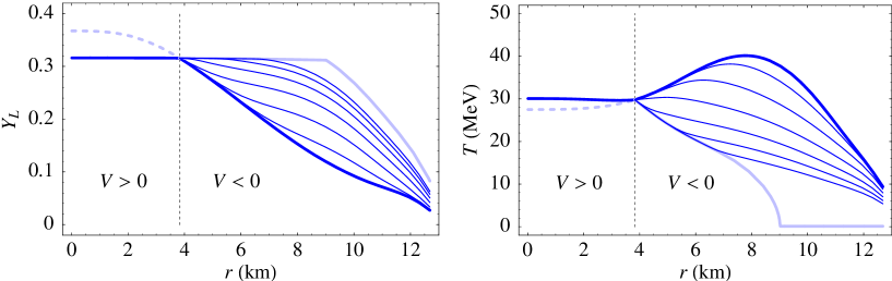
Figure 3: Lepton fraction and temperature profiles in the initial phase of the evolution. The thick dashed lines (dark solid in the $V<0$ region) represent the initial profiles. The dark thick lines show the profiles at the end of the neutrino escape phase. The thin lines show the effect of antineutrino escape 1 second later for $m^{2}\!R=10^{-(10,\,9,\,8,\,7,\,6,\,5)}\,\mathrm{eV}$. They can also be considered as the profiles at times $t=10^{-(5,\,4,\,3,\,2,\,1,\,0)}\,\mathrm{sec}\,(m^{2}\!R/(10^{-5}\,\mathrm{eV}))$ provided that $t\lesssim 1\,\mathrm{sec}$. Finally, the light thick lines show the values that would be asymptotically approached if diffusion could be indefinitely neglected.

After neutrinos in what was initially the $V>0$ region have been locked, antineutrinos loss begins to be significant in the $V<0$ region. This happens on the slower time scale $t_{\bar{\nu}}$, which depends on the position in the core. Since antineutrinos are lost, the lepton fraction $Y_{L}$, initially smaller than $Y^{0}_{L}$, grows and $V$ becomes less and less negative. Again, the essential point is whether the $V=0$ condition, or $Y_{L}=Y^{0}_{L}$, is reached before all the available energy is lost. The relevant equation is in this case

$$\frac{\partial s}{\partial Y_{L}}=-\left(\frac{F_{5/2}(-\mu_{\nu}/T)}{F_{3/2}(-\mu_{\nu}/T)}+\frac{\mu_{\nu}}{T}\right)\sim-\left(\frac{\mu_{\nu}}{T}+\frac{5}{2}\right)\;.$$ (19)

The loss turns out to be more pronounced than in the previous phase. Actually, the energy loss per unit of lepton number change is smaller, since the average antineutrino energy is $5/2\,T$ whereas the average neutrino energy was $5/7\mu_{\nu}$. However, the entropy variation is larger since the increase of $Y_{L}$ leads to an increase of the energy stored in the degenerate neutrino or electron sea at the expenses of the temperature and entropy. That is why the RHS in eq. (19) is larger than in eq. (18). Furthermore, the change in $Y_{L}$ needed to reach $Y^{0}_{L}$ is larger in the external part of the inner core, where $Y_{L}$ is lower. In order to clarify the situation, we need to numerically solve eq. (19). The result is that $V=0$ is reached before all the local energy is gone only in the inner part of the $V<0$ region. The outer part cools completely while $Y_{L}$ is still lower than $Y^{0}_{L}$, as it is apparent from Figs. 3. There, the light thick lines represent the asymptotic lepton fraction and temperature profiles that would be reached if the antineutrino escape phase continued indefinitely without diffusion. In the $r\gtrsim 9\,\mathrm{km}$ region, the asymptotic temperature profile reaches zero. Correspondingly, the maximum value of $Y_{L}$ attainable before complete cooling is not $Y^{0}_{L}$ anymore. In practice, complete cooling does not occur. The profiles reached after one second, before diffusion becomes essential, are shown by the thin lines in the $V<0$ regions of figs. 3. The lines correspond to $m^{2}\!R=10^{-(10,\,9,\,8,\,7,\,6,\,5)}\,\mathrm{eV}$. The three largest values, that are not in the parameter space we are interested in, illustrate the asymptotic behavior of the profiles. Alternatively, they can be considered as the profiles at times $t=10^{-(5,\,4,\,3,\,2,\,1,\,0)}\,\mathrm{sec}\,(m^{2}\!R/(10^{-5}\,\mathrm{eV}))$ for a given value of $m^{2}\!R$ — as long as $t\lesssim 1\,\mathrm{sec}$, of course. The $V=0$ condition is reached and antineutrinos are locked in a portion of the initially $V<0$ region which is larger the larger is $m^{2}\!R$. In a sufficiently large but finite time that would happen in all the region where the asymptotic $Y_{L}$ profile is constant and the $T$ one is non vanishing. In the outer part of the inner core, on the other hand, neither $Y^{0}_{L}$ nor the asymptotic profile will ever be reached. However, the attraction of the fixed point on $Y_{L}$ has the effect of raising the $Y_{L}$ profile, with interesting implications that will be discussed in section 3.4. The total energy loss in this phase is again a small fraction of the total available energy.

After the first, fast phase of neutrino escape and the second slower phase of antineutrino escape, diffusion begins to play a significant role. This happens on the slowest time scale $t_{\text{diff}}$. Diffusion “unlocks” the energy stored in the $V=0$ region. Some of it gets lost in the bulk, the rest diffuses out in the outer part and eventually is emitted mainly as active neutrinos. The diffusion regime however is different from the standard one that takes place in absence of transitions into the bulk. We have in this case a mixed regime in which the evolution is determined by an interplay of diffusion and escape. Let us consider first the inner part of the core, where $V=0$. Due to diffusion, the densities change, thus spoiling the $V=0$ condition. The lepton fraction decreases and $V$ becomes slightly negative. As $V$ becomes negative, though, antineutrinos start to escape in the bulk thus giving a positive contribution to $V$. At some point, the positive contribution to $V$ from conversion into bulk neutrinos will balance the negative contribution from diffusion. In this regime, some of the energy is lost in the bulk and some is diffused out. The amount of energy lost in the invisible channel turns out to be independent of $m^{2}\!R$ as long as the conversion of antineutrinos (slower than the neutrino conversion) is efficient enough to keep $|V|$ small. The evolution in such a regime is well described by a single equation for the temperature. In fact, denoting $Y_{L}=Y^{0}_{L}+\delta Y_{L}$, we have

$$V=V(\rho,T)\simeq\frac{\partial V}{\partial Y_{L}}\delta Y_{L}\;.$$ (20)

When inserted in eqs. (3.2), the previous expression allows to recover $\delta Y_{L}(\rho,T)$ from eq. (3.2a). Eq. (3.2b) then becomes

$$\begin{split}n_{B}T\frac{\partial s}{\partial t}=a_{e}\left(\vec{\nabla}\mu_{\nu}\right)^{2}&+\vec{\nabla}\cdot\left((a_{e}+a_{\mu}+a_{\tau})\frac{\pi^{2}}{6}\vec{\nabla}T^{2}\right)\\ &+\left(\mu_{\nu}-\sigma T\frac{F_{5/2}(\sigma\mu_{\nu}/T)}{F_{3/2}(\sigma\mu_{\nu}/T)}\right)\left(\vec{\nabla}\cdot\left(a_{e}~{}\vec{\nabla}\mu_{\nu}\right)-n_{B}\frac{\partial Y_{L}}{\partial t}\right)\;.\end{split}$$ (21)

Eq. (21) always holds. In the small $|V|$ limit, one can approximate $Y_{L}\simeq Y^{0}_{L}$ everywhere, in which case the equation becomes selfconsistent and the evolution becomes independent of $m^{2}\!R$. This of course will not hold forever since the efficiency of antineutrino conversion decreases as the star cools. Moreover, it certainly does not hold in the outer region where $V$ is well below zero in the first place.

In fig. 4 we show the evolution of the $Y_{L}$ and $T$ profiles that follows from eqs. (3.2) for three values of $m^{2}\!R$: $10^{-10}\,\mathrm{eV}$, $10^{-9}\,\mathrm{eV}$ and $10^{-8}\,\mathrm{eV}$. The case of no new physics is also showed in each plot for comparison (dashed lines). We do not aim at reproducing the results of the most sophisticated analysis in the literature for the latter case. However, a comparison between the solid and dashed lines in figure well illustrates the effect of new physics on the evolution. Due to neutrino conversion, $Y_{L}$ quickly drops to $Y^{0}_{L}$ in the inner part of the core. Then, on a longer time scale, diffusion further lowers $Y_{L}$, thus starting antineutrino conversion. For large values of $m^{2}\!R$, the latter is efficient enough to keep $Y_{L}$ close to $Y^{0}_{L}$ for a few seconds, until the region becomes too cool to sustain the necessary conversion. After the initial dramatic fall, the lepton fraction is higher than in the case of pure diffusion. The same happens in the outer part of the core, where the effect is more pronounced because neutrino loss never took place and $|V|$ is larger during antineutrino conversion. The lepton fraction even grows in the first second and then decreases slower than in the case of pure diffusion, at the expenses of a quicker cooling. The consequences of this effect will be discussed in the next subsection. For $m^{2}\!R=10^{-8}\,\mathrm{eV}$, the temperature in the inner core essentially never increases.

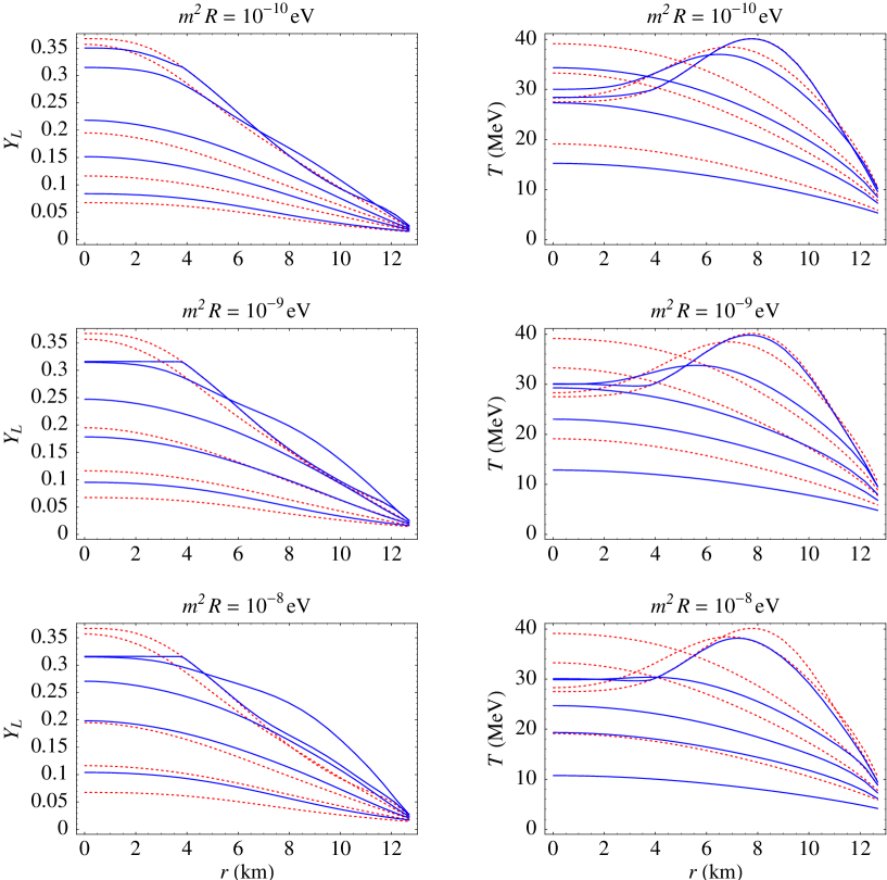
Figure 4: Lepton fraction and temperature profiles at $t=(0.01,\,1,\,10,\,20,\,40)\,\mathrm{sec}$ for different values of $m^{2}\!R$ (solid lines). The profiles for $m^{2}\!R=0$ are also shown for comparison (dashed lines).

3.4 Implications for supernova physics

Fig. 4 shows that deleptonization and cooling do take place on the same time scale as in absence of new physics despite the time scale of neutrino disappearance can be orders of magnitude faster than the diffusion one. What cannot be inferred from fig. 4 is the size of the portion of the available lepton number and energy that disappears in the bulk. Is something left to give rise to the SN 1987A neutrino signal and to revive the shock in the delayed explosion scenario? This issue is addressed in fig. 5, where the energy and lepton number lost by the inner core in the first 10 seconds are plotted against $m^{2}\!R$ and split in the component that goes into the observable neutrino flux and the component that is irremediably lost in the bulk. The latter grows with $m^{2}\!R$ but is never larger than 25% of the total. The total energy loss also grows with $m^{2}\!R$. This is just a consequence of the faster evolution of the temperature profile due to the additional loss (see fig. 4). The net effect of the growth of both the total and the invisible energy loss is that the energy emitted in the visible channel in the first 10 seconds (as well as in the following 10 seconds) remains within 10% of the $m^{2}\!R=0$ value.

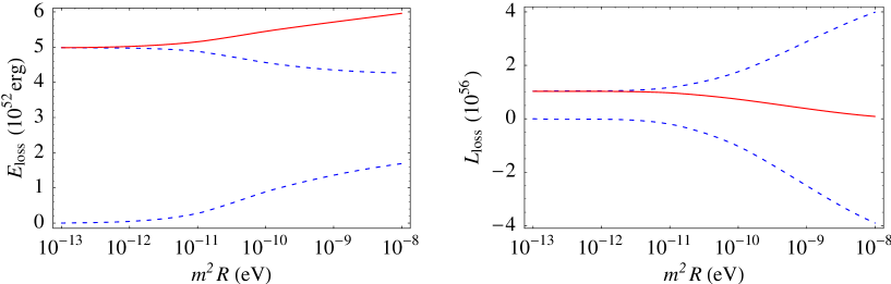
Figure 5: Energy and lepton number loss in the first 10 seconds. The total loss (solid lines) is shown together with its visible (upper dashed lines) and invisible (lower dashed lines) components as a function of $m^{2}\!R$.

The lepton number lost in the bulk in the first 10 seconds is negative, a consequence of the dominance of the antineutrino escape phase. The reluctance of the lepton fraction to get away from the $V=0$ value shows in fig. 5 in the reduction of the total lepton number loss with $m^{2}\!R$. It is also apparent how the large negative loss in the invisible channel translates into an enhancement up to a factor four of the emitted lepton number. Fig. 7 shows that the enhancement takes place on the time scale of the initial antineutrino loss rate and is therefore effective already in the first second.

The enhancement of the emitted lepton number has interesting consequences on the SN phenomenology. In order to discuss them, we first comment on the temperature of the neutrinosphere and the spectrum of the neutrino flux. A quantitative analysis of this and the following issues would require solving the evolution of the mantle, which is beyond the scope of this paper. We will therefore confine ourselves to some qualitative considerations. The disappearance probability is negligible at the density and temperature $T_{\nu}$ of the neutrinosphere, thus the latter can hardly be affected. Moreover, $T_{\nu}$ might even increase due to compressional heating until the mantle settles. The faster inner core cooling will therefore affect $T_{\nu}$ only later on. Finally, as the temperature of the neutrinosphere decreases, the neutrino mean free path grows and the neutrinosphere moves in the hotter interior, partially compensating the temperature change. We do not expect the spectrum of the neutrino flux to be significantly affected either.

The composition of the neutrino flux depends in first approximation on $T_{\nu}$ and on the energy radiated per unit of lepton number. Neglecting the difference among the neutrino spectra [25], the number of neutrinos emitted per unit of lepton number is $N\sim kE/(LT_{\nu})$, where $E$ is the energy radiated with the lepton number $L$ and $k$ characterizes the shape of the energy spectrum at the neutrinosphere. In absence of new physics one has $N\sim 10$. Since the total electron lepton number of those neutrinos must be 1, there is a slight prevalence of electron neutrinos over the other species. Consider now our situation in the extreme limit $m^{2}\!R=10^{-8}\,\mathrm{eV}$. The lepton number emitted in say the first second is 4–5 times larger than in the standard case, while the energy emitted is about the same. Each electron neutrino emitted will be therefore accompanied in average by only a couple of neutrinos of other species. Such a peculiar neutrino flux composition could be indirectly observed in the existing neutrino detectors when the signal of a SN explosion in our galaxy will reach us.

The prevalence of electron neutrinos in the neutrino flux for large $m^{2}\!R$ has two further consequences. First, it reduces the electron antineutrino component, which is constrained by the SN 1987A signal. Moreover, the electron neutrinos are much more effective than muon or tau neutrinos in depositing energy in the matter outside the neutrinosphere. As a consequence, a larger $\nu_{e}$ component might help a stalling shock in ejecting the SN envelope. In fact, the heating rate of matter irradiated by a hotter $\nu_{e}$ flux is proportional to $T_{\nu}^{2}$, which we expect not to be significantly affected by a large $m^{2}\!R$, and to the $\nu_{e}$ luminosity. As the left panel of fig. 5 shows, the total luminosity in all neutrino species (integrated over 10 seconds, but the same holds for the luminosity itself) is not significantly affected. Therefore, an increase of the $\nu_{e}$ component has the effect of increasing the $\nu_{e}$ luminosity and, in turn, the heating rate. The enhancement can be significant and is only limited by the reduction of the $\bar{\nu}_{e}$ flux and the effect on r-processes one is willing to accept.

Figure 6: Enhancement of the lepton number flux over the $m^{2}\!R=0$ case. The five lines correspond to $m^{2}\!R=10^{-(12,\,11,\,10,\,9,\,8)}\,\mathrm{eV}$. The enhancement grows with $m^{2}\!R$.

Figure 7: Limits on the amplitude of $\nu_{e}$, $\bar{\nu}_{e}$ and $\nu_{\mu,\tau}$ or $\bar{\nu}_{\mu,\tau}$ oscillations into an invisible channel as functions of the squared mass difference ${\Delta m^{2}}$.

4 “Conventional” invisible channels

Before concluding, we discuss the limits on conventional (non self-limiting) invisible cooling channels. This simple application of the formalism set up in the previous section is relevant to our discussion because it provides the condition under which subleading contribution to the disappearance probability are under control.

Let $P_{\nu}(L,E)$ be the probability that a neutrino of type $\nu=\nu_{e},\nu_{\mu},\nu_{\tau},\bar{\nu}_{e},\bar{\nu}_{\mu},\bar{\nu}_{\tau}$ with energy $E$ disappears in an invisible channel while traveling a distance $L$ and let us assume that there is no reappearance. In order to obtain a limit on $P_{\nu}$, we compare the consequent lepton number loss rate with the diffusion one. The simplest case is that of a power-law disappearance probability $P_{\nu}(L,E)=P_{0}(L/L_{0})^{\alpha}(E/E_{0})^{\beta}$. For example, the mixing with a tower of KK states gives rise to a contribution to the escape probability which is essentially constant in the relevant range for $L$, $E$: $P_{\nu_{e},\bar{\nu}_{e}}\sim(mR)^{2}$.

The neutrino number density loss rate is

$$\Gamma_{\nu}=\int\frac{d\vec{p}}{(2\pi)^{3}}\frac{\left\langle P\right\rangle_{E}}{\lambda_{\nu}(E)}f_{\nu}(E)\,,$$ (22)

where $\left\langle P\right\rangle=\int^{\infty}_{0}dxP(x\lambda_{\nu}(E),E)e^{-x}$ is the average over the distance traveled of the disappearance probability. In the case of a power law probability and within the approximations discussed in Section 3.1, one has

$$\Gamma_{\nu}=\frac{\Gamma(\alpha+1)}{12\pi^{4}a_{\nu}}\,T^{5}F_{4+\beta-2\alpha}\left(\frac{\mu_{\nu}}{T}\right)\,,$$ (23)

where $a_{\nu}=\lambda_{\nu}E^{2}/(6\pi^{2})$. By definition of $t_{\text{diff}}$, the diffusion rate is $\Gamma_{\text{diff}}=n_{B}\partial Y_{L}/\partial t=n_{B}Y_{L}/t_{\text{diff}}$. The limit on the probability following from $\Gamma_{\nu}<\Gamma_{\text{diff}}$ reflects the abundance of the neutrino type considered,

$$P_{\nu}(\lambda(\mu_{\nu}),\mu_{\nu}) <2\cdot 10^{-11}a_{\alpha\beta}\left(\frac{200\,\mathrm{MeV}}{\mu_{\nu}}\right)^{5}\frac{\rho}{\rho_{0}}\frac{Y_{L}}{0.3}\frac{10\,\mathrm{sec}}{t_{\text{diff}}} \nu=\nu_{e}$$ for (24a)

$$P_{\nu}(\lambda(T),T) <1.5\cdot 10^{-8}b_{\alpha\beta}\left(\frac{30\,\mathrm{MeV}}{T}\right)^{5}\frac{\rho}{\rho_{0}}\frac{Y_{L}}{0.3}\frac{10\,\mathrm{sec}}{t_{\text{diff}}} \nu=\nu_{\mu,\tau} \bar{\nu}_{\mu,\tau}$$ for or (24b)

$$P_{\nu}(\lambda(T),T) <3\cdot 10^{-6}b_{\alpha\beta}\,e^{(\mu_{\nu}/T-20/3)}\left(\frac{30\,\mathrm{MeV}}{T}\right)^{5}\frac{\rho}{\rho_{0}}\frac{Y_{L}}{0.3}\frac{10\,\mathrm{sec}}{t_{\text{diff}}} \text{for $\nu=\bar{\nu}_{e}$}\,,$$ (24c)

where $a_{\alpha\beta}=(5+\beta-2\alpha)/(5\Gamma(\alpha+1))$, $b_{\alpha\beta}=24/(\Gamma(5+\beta-2\alpha)\Gamma(\alpha+1))$ are numerical coefficients normalized to $a_{00}=b_{00}=1$. In particular, in the case of a constant electron neutrino disappearance probability $P_{\nu_{e}}=(mR)^{2}$ we get the limit $mR\lesssim 0.5\cdot 10^{-5}(200\,\mathrm{MeV}/\mu_{\nu})^{5/2}(10\,\mathrm{sec}/t_{\text{diff}})$ that we used to determine the conservative upper bound $m^{2}\!R\lesssim 10^{-8}\,\mathrm{eV}$.

For completeness, we also give the limit on the amplitude of a simple oscillation probability $P_{\nu}(L,E)=A\sin^{2}({\Delta m^{2}}L/(4E))$ into an invisible channel. The limit on $A$ as a function of ${\Delta m^{2}}$ for the case of $\nu_{e}$, $\bar{\nu}_{e}$ and $\nu_{\mu,\tau}$ or $\bar{\nu}_{\mu,\tau}$ oscillations is plotted in Fig. 7 for $\rho=\rho_{0}$, $Y=0.3$, $t_{\text{diff}}=10\,\mathrm{sec}$, $\mu_{\nu}=200\,\mathrm{MeV}$ and $T=30\,\mathrm{MeV}$.

5 Summary

The supernova plays an important role in the phenomenology of a possible mixing between SM neutrinos and fermions propagating in the bulk of large extra dimensions. We studied both the constraints on such a mixing following from the necessity of avoiding unacceptable energy loss and the implications for supernova physics. We considered the simple case of mixing between the electron neutrino and a single KK tower of 5D bulk neutrinos. The parameter space where interesting effects arise is quite broad, with the size of the extra dimension in the range $10^{-2}\,\mathrm{eV}\lesssim 1/R\lesssim 1\,\mathrm{keV}$ and the mixing mass parameter $m$ such that $10^{-12}\,\mathrm{eV}\lesssim m^{2}\!R\lesssim 10^{-8}\,\mathrm{eV}$ and $mR\lesssim 10^{-5}$. The interplay of neutrino diffusion and conversion into bulk neutrinos has an important role in the phenomenology we study and requires taking into account the relevant aspects of neutrino transport, which we did in the context of a simplified model of the protoneutron star core.

Due to the large number of available states and especially to matter effects, the rate at which neutrino disappearance in the bulk cools the protoneutron star is initially dangerously high. If taken at face value, such a rate would set quite a stringent bound on $m^{2}\!R$, $m^{2}\!R\lesssim 10^{-12}\,\mathrm{eV}$ in the case of neutrino conversion. However, the disappearance rate quickly reduces itself to acceptable values. This happens for different reasons. In the region where the MSW potential $V$ is positive, neutrinos escape in the bulk and the lepton fraction quickly drops to the value $Y^{0}_{L}\simeq 0.3$ at which $V=0$, thus stopping the potentially most dangerous MSW enhanced conversion before a significant amount of energy is lost. Then, on a much slower time scale, neutrino diffusion spoils the $V=0$ condition and unlocks the energy frozen in what was initially the $V>0$ region. The potential becomes slightly negative and antineutrinos start escaping in the bulk to restore the $V=0$ condition. This feedback keeps $Y_{L}$ close to $Y^{0}_{L}$ until the temperature becomes too low to sustain the necessary antineutrino escape rate. In the region where the potential was initially negative, neutrino conversion never takes place. The initial loss rate is smaller because of the much lower antineutrino density. Still, it would be too high for large values of $m^{2}\!R$. However, in the inner part of the $V<0$ region the antineutrino loss stops itself by drawing $V$ up to zero before all the local energy is lost, analogously to the $V>0$ case. In the outer part of the $V<0$ region, there is not enough energy to reach $V=0$. However, the conversion again controls itself. This happens this time because the energy loss, proportional to $T^{7/2}$, becomes less and less effective as the region cools.

The described mechanism allows to gain four orders of magnitude in the allowed range for $m^{2}\!R$ ($10^{-12}\,\mathrm{eV}\rightarrow 10^{-8}\,\mathrm{eV}$). In the subsequent four orders of magnitudes, the MSW enhanced conversion would still be under control but what were previously neglected as subleading contributions to the oscillation probability become too large. Such contributions, as well as the limits on other “conventional” invisible cooling channels, were discussed in Section 4. In the gained portion of the parameter space, the implications for supernova physics are particularly interesting. Although compatible with the SN 1987A signal, the evolution of the protoneutron star is significantly affected, especially for large values of $m^{2}\!R$. Deleptonization and cooling take place on the same time scale as in absence of new physics. However, the reluctance of the lepton fraction to get away from $Y^{0}_{L}\sim 0.3$ slows the deleptonization, while the energy loss accelerates the cooling. Up to a fourth of the energy lost by the protoneutron star goes to the bulk but the total luminosity in all neutrino species turns out to be approximately the same as in the standard case, at least in the first 20 seconds. Antineutrinos escape in the bulk in the effort of keeping $Y_{L}$ close to $Y^{0}_{L}$, which boosts the lepton number radiated from the neutrinosphere. A quantitative study of the consequences of such an enhancement would require solving the evolution of the mantle. However, we expect it to result in an enhancement of the $\nu_{e}$ component of the neutrino flux and therefore of the $\nu_{e}$ luminosity, an effect observable in the existing neutrino detectors. Since we expect the temperature of the neutrinosphere not to be significantly affected, the energy deposition in a possibly stalling shock would also be enhanced at the expenses of a smaller $\bar{\nu}_{e}$ luminosity.

The exotic phenomenology discussed in this paper represents an example of how the standard ideas about protoneutron star evolution could be affected in an unexpected way by the presence of new physics.

References

- [1] Q. R. Ahmad et al. [SNO Collaboration], Phys. Rev. Lett. 87 (2001) 071301 [arXiv:nucl-ex/0106015]; Q. R. Ahmad et al. [SNO Collaboration], Phys. Rev. Lett. 89 (2002) 011301 [arXiv:nucl-ex/0204008]; Q. R. Ahmad et al. [SNO Collaboration], Phys. Rev. Lett. 89 (2002) 011302 [arXiv:nucl-ex/0204009].
- [2] K. R. Dienes, E. Dudas and T. Gherghetta, Nucl. Phys. B 557 (1999) 25 [arXiv:hep-ph/9811428]; N. Arkani-Hamed, S. Dimopoulos, G. R. Dvali and J. March-Russell, Phys. Rev. D 65 (2002) 024032 [arXiv:hep-ph/9811448].
- [3] G. R. Dvali and A. Y. Smirnov, Nucl. Phys. B 563 (1999) 63 [arXiv:hep-ph/9904211].
- [4] I. Antoniadis, Phys. Lett. B 246 (1990) 377; J. D. Lykken, Phys. Rev. D 54 (1996) 3693 [arXiv:hep-th/9603133]; N. Arkani-Hamed, S. Dimopoulos and G. R. Dvali, Phys. Lett. B 429 (1998) 263 [arXiv:hep-ph/9803315]; I. Antoniadis, N. Arkani-Hamed, S. Dimopoulos and G. R. Dvali, Phys. Lett. B 436 (1998) 257 [arXiv:hep-ph/9804398].
- [5] A. Pomarol and M. Quiros, Phys. Lett. B 438 (1998) 255 [arXiv:hep-ph/9806263]; R. Barbieri, L. J. Hall and Y. Nomura, Phys. Rev. D 63 (2001) 105007 [arXiv:hep-ph/0011311].
- [6] K. Hirata et al. [KAMIOKANDE-II Collaboration], Phys. Rev. Lett. 58 (1987) 1490; R. M. Bionta et al., Phys. Rev. Lett. 58 (1987) 1494.
- [7] G. G. Raffelt, Ann. Rev. Nucl. Part. Sci. 49 (1999) 163 [arXiv:hep-ph/9903472].
- [8] N. Arkani-Hamed, S. Dimopoulos and G. R. Dvali, Phys. Rev. D 59 (1999) 086004 [arXiv:hep-ph/9807344]; T. Han, J. D. Lykken and R. J. Zhang, Phys. Rev. D 59 (1999) 105006 [arXiv:hep-ph/9811350]; S. Cullen and M. Perelstein, Phys. Rev. Lett. 83 (1999) 268 [arXiv:hep-ph/9903422]; C. Hanhart, D. R. Phillips, S. Reddy and M. J. Savage, Nucl. Phys. B 595 (2001) 335 [arXiv:nucl-th/0007016]; C. Hanhart, J. A. Pons, D. R. Phillips and S. Reddy, Phys. Lett. B 509 (2001) 1 [arXiv:astro-ph/0102063].
- [9] A. D. Dolgov, S. H. Hansen, G. Raffelt and D. V. Semikoz, Nucl. Phys. B 580 (2000) 331 [arXiv:hep-ph/0002223].
- [10] R. Barbieri, P. Creminelli and A. Strumia, Nucl. Phys. B 585 (2000) 28 [arXiv:hep-ph/0002199].
- [11] H. Nunokawa, J. T. Peltoniemi, A. Rossi and J. W. Valle, Phys. Rev. D 56 (1997) 1704 [arXiv:hep-ph/9702372].
- [12] A. Lukas, P. Ramond, A. Romanino and G. G. Ross, JHEP 0104 (2001) 010 [arXiv:hep-ph/0011295].
- [13] For general reviews and extensive references, see H. A. Bethe, Rev. Mod. Phys. 62 (1990) 801; G. G. Raffelt, “ Stars and as laboratories for fundamental physics: The astrophysics of neutrinos, axions, and other weakly interacting particles,” Chicago Univ.Press, Chicago, 1996.
- [14] J. M. Lattimer, “The Nuclear Equation of State and Supernovae,” in “Nuclear Equation of State”, ed. A. Ansari and L. Satpathy (World Scientific, Singapore), pp. 83-208 (1996); M. Prakash, J. M. Lattimer, J. A. Pons, A. W. Steiner and S. Reddy, “Evolution of a Neutron Star From its Birth to Old Age,” Lect. Notes Phys. 578 (2001) 364 [arXiv:astro-ph/0012136]; H. T. Janka, K. Kifonidis and M. Rampp, “Supernova explosions and neutron star formation,” Lect. Notes Phys. 578 (2001) 333 [arXiv:astro-ph/0103015].
- [15] S. Yamada, H-Th. Janka and H. Suzuki, A.& A. 344 (1999) 533-550 [arXiv:astro-ph/9809009]; M. Rampp and H. T. Janka, Astrophys. J. 539 (2000) L33 [arXiv:astro-ph/0005438]; A. Mezzacappa, M. Liebendorfer, O. E. Messer, W. R. Hix, F. K. Thielemann and S. W. Bruenn, Phys. Rev. Lett. 86 (2001) 1935 [arXiv:astro-ph/0005366]; M. Liebendorfer, A. Mezzacappa, F. K. Thielemann, O. E. Messer, W. R. Hix and S. W. Bruenn, Phys. Rev. D 63 (2001) 103004 [arXiv:astro-ph/0006418].
- [16] M. Rampp, E. Mueller and M. Ruffert, A.& A. 332 (1998) 969-983 [arXiv:astro-ph/9711122].
- [17] For example, convective motions have been considered in M. Herant, W. Benz, W. R. Hix, C. L. Fryer and S. A. Colgate, Astrophys. J. 435 (1994) 339 [arXiv:astro-ph/9404024]; A. Burrows, J. Hayes and B. A. Fryxell, Astrophys. J. 450 (1995) 830 [arXiv:astro-ph/9506061]; rotation in R. Mönchmeyer, G. Schaefer, E. Mueller and R. E. Kates, A.& A. 246 (1991) 417-440; rotation and magnetic fields in J. M. Leblanc and J. R. Wilson, Astrophys. J. 450 (1995) 830.
- [18] See, for example, polarization spectrometry results in D. C. Leonard, A. V. Filippenko, D. R. Ardila and M. S. Brotherton, Astrophys. J. 553 (2001) 861 [arXiv:astro-ph/0009285]; L. Wang, D. A. Howell, P. Höflich, and J. C. Wheeler, Astrophys. J. 550 (2001) 1030.
- [19] A. Lukas, P. Ramond, A. Romanino and G. G. Ross, Phys. Lett. B 495 (2000) 136 [arXiv:hep-ph/0008049].
- [20] A. E. Faraggi and M. Pospelov, Phys. Lett. B 458 (1999) 237 [arXiv:hep-ph/9901299]; R. N. Mohapatra, S. Nandi and A. Perez-Lorenzana, Phys. Lett. B 466 (1999) 115 [arXiv:hep-ph/9907520]; A. Ioannisian and A. Pilaftsis, Phys. Rev. D 62 (2000) 066001 [arXiv:hep-ph/9907522]; A. Lukas and A. Romanino, arXiv:hep-ph/0004130; K. R. Dienes and I. Sarcevic, Phys. Lett. B 500 (2001) 133 [arXiv:hep-ph/0008144]; A. Lukas, P. Ramond, A. Romanino and G. G. Ross, Int. J. Mod. Phys. A 16S1C (2001) 934; D. O. Caldwell, R. N. Mohapatra and S. J. Yellin, Phys. Rev. Lett. 87 (2001) 041601 [arXiv:hep-ph/0010353]; A. S. Dighe and A. S. Joshipura, Phys. Rev. D 64 (2001) 073012 [arXiv:hep-ph/0105288]; A. De Gouvea, G. F. Giudice, A. Strumia and K. Tobe, Nucl. Phys. B 623 (2002) 395 [arXiv:hep-ph/0107156]; H. Davoudiasl, P. Langacker and M. Perelstein, Phys. Rev. D 65 (2002) 105015 [arXiv:hep-ph/0201128].
- [21] L. J. Hall and D. R. Smith, Phys. Rev. D 60 (1999) 085008 [arXiv:hep-ph/9904267]; S. Hannestad, Phys. Rev. D 64 (2001) 023515 [arXiv:hep-ph/0102290].
- [22] A. Burrows, T. J. Mazurek, J. M. Lattimer, Astrophys. J. 251 (1981) 325; A. Burrows and J. M. Lattimer, Astrophys. J. 307 (1986) 178.
- [23] S. Reddy, M. Prakash and J. M. Lattimer, Phys. Rev. D 58 (1998) 013009 [arXiv:astro-ph/9710115].
- [24] W. Keil and H. T. Janka, Astron. Astrophys. 296 (1995) 145; K. Sumiyoshi, H. Suzuki and H. Toki, Astron. Astrophys. 303 (1995) 475 [arXiv:astro-ph/9506024]; J. A. Pons, S. Reddy, M. Prakash, J. M. Lattimer and J. A. Miralles, Astrophys. J. 513 (1999) 780 [arXiv:astro-ph/9807040].
- [25] For a recent discussion of spectra formation, see e.g. M. T. Keil et al., “Monte Carlo Study of Supernova Neutrino Spectra Formation,” [arXiv:astro-ph/0208035].