PCCF-RI-02-08

ADP-02-81/T520

Enhanced direct $CP$ violation in $B^{\pm,0}\rightarrow\pi^{+}\pi^{-}K^{\pm,0}$

O. Leitner^1,2, X.-H. Guo¹, A.W. Thomas^1
1 Department of Physics and Mathematical Physics, and

Special Research Center for the Subatomic Structure of Matter,

University of Adelaide, Adelaide 5005, Australia

² Laboratoire de Physique Corpusculaire, Université Blaise Pascal,

CNRS/IN2P3, 24 avenue des Landais, 63177 Aubière Cedex, France

We investigate in a phenomenological way, direct $CP$ violation in the hadronic decays $B^{\pm,0}\rightarrow\pi^{+}\pi^{-}K^{\pm,0}$ where the effect of $\rho-\omega$ mixing is included. If $N_{c}^{eff}$ (the effective parameter associated with factorization) is constrained using the most recent experimental branching ratios (to $\rho^{0}K^{0},\rho^{\pm}K^{\mp},\rho^{\pm}K^{0},\rho^{0}K^{\pm}$ and $\omega K^{\pm}$) from the BABAR, BELLE and CLEO Collaborations, we get a maximum $CP$ violating asymmetry, $a_{max}$, in the range $-25\%$ to $+49\%$ for $B^{-}\rightarrow\pi^{+}\pi^{-}K^{-}$ and $-24\%$ to $+55\%$ for ${\bar{B}}^{0}\rightarrow\pi^{+}\pi^{-}{\bar{K}}^{0}$. We also find that $CP$ violation is strongly dependent on the Cabibbo-Kobayashi-Maskawa matrix elements. Finally, we show that the sign of $\sin\delta$ is always positive in the allowed range of $N_{c}^{eff}$ and hence, a measurement of direct $CP$ violation in $B^{\pm,0}\rightarrow\pi^{+}\pi^{-}K^{\pm,0}$ would remove the mod$(\pi)$ ambiguity in ${\rm arg}\left[-\frac{V_{ts}V_{tb}^{\star}}{V_{us}V_{ub}^{\star}}\right]$.

PACS Numbers: 11.30.Er, 12.39.-x, 13.25.Hw.

1 Introduction

The study of $CP$ violation in $B$ decays is one of the most important aims for the $B$ factories. The relative large $CP$ violating effects expected in $B$ meson decays should provide efficient tests of the standard model through the Cabibbo-Kobayashi-Maskawa (CKM) matrix. It is usually assumed that a nonzero imaginary phase angle, $\eta$, is responsible for the $CP$ violating phenomena. This is why, in the past few years, numerous theoretical studies and experiments have been conducted in the $B$ meson system [1, 2] in order to reduce uncertainties in calculations (e.g. CKM matrix elements, hadronic matrix elements and nonfactorizable effects) and increase our understanding of $CP$ violation within the standard model framework.
Direct $CP$ violating asymmetries in $B$ decays occur through the interference of at least two amplitudes with different weak phase $\phi$ and strong phase $\delta$. In order to extract the weak phase (which is determined by the CKM matrix elements) through the measurement of a $CP$ violating asymmetry, one must know the strong phase $\delta$ and this is usually not well determined. In addition, in order to have a large signal, we have to appeal to some phenomenological mechanism to obtain a large $\delta$. The charge symmetry violating mixing between $\rho^{0}$ and $\omega$ can be extremely important in this regard. In particular, it can lead to a large $CP$ violation in $B$ decays, such as $B^{\pm,0}\rightarrow\rho^{0}(\omega)K^{\pm,0}\rightarrow\pi^{+}\pi^{-}K^{\pm,0}$, because the strong phase passes through $90^{o}$ at the $\omega$ resonance [3, 4, 5].
We have collected the latest data for $b$ to $s$ transitions concentrating on the CLEO, BABAR and BELLE branching ratio results in our approach. The aim of the present work is multiple. The main one is to constrain the $CP$ violating calculation in $B^{\pm,0}\rightarrow\rho^{0}(\omega)K^{\pm,0}\rightarrow\pi^{+}\pi^{-}K^{\pm,0}$, including $\rho-\omega$ mixing and using the most recent experimental data for $B\rightarrow\rho K$ decays. The second one is to extract consistent constraints for $B$ decays into $\rho(PS)$ where $PS$ can be either $\pi$ or $K$. In order to extract the strong phase $\delta$, we shall use the factorization approach, in which the hadronic matrix elements of operators are saturated by vacuum intermediate states. Moreover, we approximate non-factorizable effects by introducing an effective number of colors, $N_{c}^{eff}$.
In this paper we investigate five phenomenological models with different weak form factors and determine the $CP$ violating asymmetry, $a$, for $B^{\pm,0}\rightarrow\rho^{0}(\omega)K^{\pm,0}\rightarrow\pi^{+}\pi^{-}K^{\pm,0}$ in these models. We select models which are consistent with all the data and determine the allowed range for $N_{c}^{eff}$ ($0.66(0.61)<N_{c}^{eff}<2.84(2.82)$). Then, we study the sign of $\sin\delta$ in this range of $N_{c}^{eff}$ for all these models. We also discuss the model dependence of our results in detail.
The remainder of this paper is organized as it follows. In Section 2, we present the form of the effective Hamiltonian which is based on the operator product expansion, together with the values of the corresponding Wilson coefficients. In Section 3, we give the phenomenological formalism for the $CP$ violating asymmetry in decay processes including $\rho-\omega$ mixing, where all aspects of the calculation of direct $CP$ violation, the CKM matrix, $\rho-\omega$ mixing, factorization and form factors are discussed in detail. In Section 4, we list all the numerical inputs which are needed for calculating the asymmetry, $a$, in $B^{\pm,0}\rightarrow\rho^{0}(\omega)K^{\pm,0}\rightarrow\pi^{+}\pi^{-}K^{\pm,0}$. Section 5 is devoted to results and discussions for these decays. In Section 6, we calculate branching ratios for decays such as $B^{\pm,0}\rightarrow\rho^{\pm,0}K^{\pm,0}$ and $B^{\pm}\rightarrow\omega K^{\pm}$ as well, and present numerical results over the range of $N_{c}^{eff}$ which is allowed by experimental data from the CLEO, BABAR, and BELLE Collaborations. In the last section, we summarize our results and determine the allowed range of $N_{c}^{eff}$ which is consistent with data for both $\rho\pi$ and $\rho K$ decays. Uncertainties in our approach and conclusions are also discussed in this section.

2 The effective Hamiltonian

2.1 Operator product expansion

Operator product expansion (OPE) [6] is a useful tool introduced to analyze the weak interaction of quarks. Defining the decay amplitude $A(M\rightarrow F)$ as

$$A(M\rightarrow F)\propto C_{i}(\mu)\langle F|O_{i}(\mu)|M\rangle\ ,$$ (1)

where $C_{i}(\mu)$ are the Wilson coefficients (see Section 2.2) and $O_{i}(\mu)$ the operators given by the OPE, one sees that OPE separates the calculation of the amplitude, $A(M\rightarrow F)$, into two distinct physical regimes. One is related to hard or short-distance physics, represented by $C_{i}(\mu)$ and calculated by a perturbative approach. The other is the soft or long-distance regime. This part must be treated by non-perturbative approaches such as the $1/N$ expansion [7], QCD sum rules [8] or hadronic sum rules.

The operators, $O_{i}$, are local operators which can be written in the general form:

$$O_{n}=({\bar{q}}_{i}\Gamma_{n1}q_{j})({\bar{q}}_{k}\Gamma_{n2}q_{l})\ ,$$ (2)

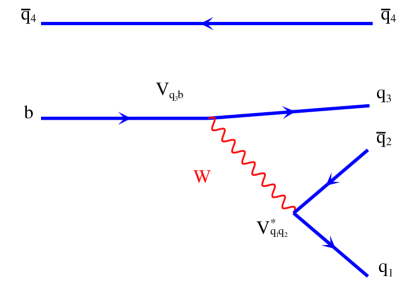
Figure 1: Tree diagram, for $B$ decays.

where $\Gamma_{n1}$ and $\Gamma_{n2}$ denote a combination of gamma matrices and $q$ the quark flavor. They should respect the Dirac structure, the color structure and the types of quarks relevant for the decay being studied. They can be divided into two classes according to topology: tree operators ($O_{1},O_{2}$), and penguin operators ($O_{3}$ to $O_{10}$). For tree contributions ($W^{\pm}$ is exchanged), the Feynman diagram is shown Fig. 1. The current-current operators related to the tree diagram are the following:

$$O_{1}^{s} =\bar{q}_{\alpha}\gamma_{\mu}(1-\gamma{{}_{5}})u_{\beta}\bar{s}_{\beta}\gamma^{\mu}(1-\gamma{{}_{5}})b_{\alpha}\ ,$$

$$O_{2}^{s} =\bar{q}\gamma_{\mu}(1-\gamma{{}_{5}})u\bar{s}\gamma^{\mu}(1-\gamma{{}_{5}})b\ ,$$ (3)

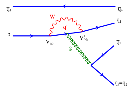
Figure 2: QCD penguin diagram, for $B$ decays.

where $\alpha$ and $\beta$ are the color indices. The penguin terms can be divided into two sets. The first is from the QCD penguin diagrams (gluons are exchanged) and the second is from the electroweak penguin diagrams ($\gamma$ and $Z^{0}$ exchanged). The Feynman diagram for the QCD penguin diagram is shown in Fig. 2 and the corresponding operators are written as follows:

$$O_{3} =\bar{q}\gamma_{\mu}(1-\gamma{{}_{5}})b\sum_{q\prime}\bar{q}^{\prime}\gamma^{\mu}(1-\gamma{{}_{5}})q^{\prime}\ ,$$

$$O_{4} =\bar{q}_{\alpha}\gamma_{\mu}(1-\gamma{{}_{5}})b_{\beta}\sum_{q\prime}\bar{q}^{\prime}_{\beta}\gamma^{\mu}(1-\gamma{{}_{5}})q^{\prime}_{\alpha}\ ,$$ (4)

$$O_{5} =\bar{q}\gamma_{\mu}(1-\gamma{{}_{5}})b\sum_{q^{\prime}}\bar{q}^{\prime}\gamma^{\mu}(1+\gamma{{}_{5}})q^{\prime}\ ,$$

$$O_{6} =\bar{q}_{\alpha}\gamma_{\mu}(1-\gamma{{}_{5}})b_{\beta}\sum_{q^{\prime}}\bar{q}^{\prime}_{\beta}\gamma^{\mu}(1+\gamma{{}_{5}})q^{\prime}_{\alpha}\ ,$$ (5)

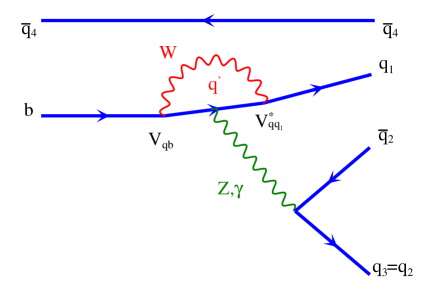
Figure 3: Electroweak-penguin diagram, for $B$ decays.

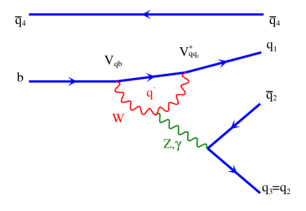
Figure 4: Electroweak-penguin diagram (coupling between $Z,\gamma$ and $W$), for $B$ decays.

where $q^{\prime}=u,d,s,c$. Finally, the electroweak penguin operators arise from the two Feynman diagrams represented in Fig. 3 ($Z,\gamma$ exchanged from a quark line) and Fig. 4 ($Z,\gamma$ exchanged from the $W$ line). They have the following expressions:

$$O_{7} =\frac{3}{2}\bar{q}\gamma_{\mu}(1-\gamma{{}_{5}})b\sum_{q^{\prime}}e_{q^{\prime}}\bar{q}^{\prime}\gamma^{\mu}(1+\gamma{{}_{5}})q^{\prime}\ ,$$

$$O_{8} =\frac{3}{2}\bar{q}_{\alpha}\gamma_{\mu}(1-\gamma{{}_{5}})b_{\beta}\sum_{q^{\prime}}e_{q^{\prime}}\bar{q}^{\prime}_{\beta}\gamma^{\mu}(1+\gamma{{}_{5}})q^{\prime}_{\alpha}\ ,$$

$$O_{9} =\frac{3}{2}\bar{q}\gamma_{\mu}(1-\gamma{{}_{5}})b\sum_{q^{\prime}}e_{q^{\prime}}\bar{q}^{\prime}\gamma^{\mu}(1-\gamma{{}_{5}})q^{\prime}\ ,$$

$$O_{10} =\frac{3}{2}\bar{q}_{\alpha}\gamma_{\mu}(1-\gamma{{}_{5}})b_{\beta}\sum_{q^{\prime}}e_{q^{\prime}}\bar{q}^{\prime}_{\beta}\gamma^{\mu}(1-\gamma{{}_{5}})q^{\prime}_{\alpha}\ ,$$ (6)

where $e_{q^{\prime}}$ denotes the electric charge of $q^{\prime}$.

2.2 Wilson coefficients

As we mentioned in the preceding subsection, the Wilson coefficients [9], $C_{i}(\mu)$, represent the physical contributions from scales higher than $\mu$ (the OPE describes physics for scales lower than $\mu$). Since QCD has the property of asymptotic freedom, they can be calculated in perturbation theory. The Wilson coefficients include contributions of all heavy particles, such as the top quark, the $W$ bosons, and the charged Higgs boson. Usually, the scale $\mu$ is chosen to be of order $O(m_{b})$ for $B$ decays. Wilson coefficients have been calculated to the next-to-leading order (NLO). The evolution of $C(\mu)$ (the matrix that includes $C_{i}(\mu)$) is given by,

$$C(\mu)=U(\mu,M_{W})C(M_{W})\ ,$$ (7)

where $U(\mu,M_{W})$ is the QCD evolution matrix:

$$U(\mu,M_{W})=\biggl{[}1+\frac{\alpha_{s}(\mu)}{4\pi}J\biggr{]}U^{0}(\mu,M_{W})\biggl{[}1-\frac{\alpha_{s}(M_{W})}{4\pi}J\biggr{]}\ ,$$ (8)

with $J$ the matrix summarizing the next-to-leading order corrections and $U^{0}(\mu,M_{W})$ the evolution matrix in the leading-logarithm approximation. Since the strong interaction is independent of quark flavor, the $C(\mu)$ are the same for all $B$ decays. At the scale $\mu=m_{b}=5$ GeV, $C(\mu)$ take the values summarized in Table 1 [10, 11].

To be consistent, the matrix elements of the operators, $O_{i}$, should also be renormalized to the one-loop order. This results in the effective Wilson coefficients, $C_{i}^{\prime}$, which satisfy the constraint,

$$C_{i}(m_{b})\langle O_{i}(m_{b})\rangle=C_{i}^{\prime}{\langle O_{i}\rangle}^{tree}\ ,$$ (9)

where ${\langle O_{i}\rangle}^{tree}$ are the matrix elements at the tree level. These matrix elements will be evaluated in the factorization approach. From Eq. (9), the relations between $C_{i}^{\prime}$ and $C_{i}$ are [10, 11],

$$C_{1}^{\prime} =C_{1}\ ,\; C_{2}^{\prime} =C_{2}\ ,$$

$$C_{3}^{\prime} =C_{3}-P_{s}/3\ ,\; C_{4}^{\prime} =C_{4}+P_{s}\ ,$$

$$C_{5}^{\prime} =C_{5}-P_{s}/3\ ,\; C_{6}^{\prime} =C_{6}+P_{s}\ ,$$

$$C_{7}^{\prime} =C_{7}+P_{e}\ ,\; C_{8}^{\prime} =C_{8}\ ,$$

$$C_{9}^{\prime} =C_{9}+P_{e}\ ,\; C_{10}^{\prime} =C_{10}\ ,$$ (10)

where,

$$P_{s} =(\alpha_{s}/8\pi)C_{2}(10/9+G(m_{c},\mu,q^{2}))\ ,$$

$$P_{e} =(\alpha_{em}/9\pi)(3C_{1}+C_{2})(10/9+G(m_{c},\mu,q^{2}))\ ,$$ (11)

and

$$G(m_{c},\mu,q^{2})=4\int_{0}^{1}dxx(x-1){\rm ln}\frac{m_{c}^{2}-x(1-x)q^{2}}{\mu^{2}}\ .$$ (12)

Here $q^{2}$ is the typical momentum transfer of the gluon or photon in the penguin diagrams and $G(m_{c},\mu,q^{2})$ has the following explicit expression [12],

$$\Re e\;G=\frac{2}{3}\left({\rm ln}\frac{m_{c}^{2}}{\mu^{2}}-\frac{5}{3}-4\frac{m_{c}^{2}}{q^{2}}+\left(1+2\frac{m_{c}^{2}}{q^{2}}\right)\sqrt{1-4\frac{m_{c}^{2}}{q^{2}}}{\rm ln}\frac{1+\sqrt{1-4\frac{m_{c}^{2}}{q^{2}}}}{1-\sqrt{1-4\frac{m_{c}^{2}}{q^{2}}}}\right),$$

$$\Im m\;G=-\frac{2}{3}\left(1+2\frac{m_{c}^{2}}{q^{2}}\right)\sqrt{1-4\frac{m_{c}^{2}}{q^{2}}}\ .$$ (13)

Based on simple arguments at the quark level, the value of $q^{2}$ is chosen in the range $0.3<q^{2}/m_{b}^{2}<0.5$ [3, 4]. From Eqs. (2.2-2.2) we can obtain numerical values for $C_{i}^{\prime}$. These values are listed in Table 2, where we have taken $\alpha_{s}(m_{Z})=0.112,\;\;\;\alpha_{em}(m_{b})=1/132.2,\;\;\;m_{b}=5$ GeV, and $\;\;m_{c}=1.35$ GeV.

2.3 Effective Hamiltonian

In any phenomenological treatment of the weak decays of hadrons, the starting point is the weak effective Hamiltonian at low energy [13]. It is obtained by integrating out the heavy fields (e.g. the top quark, $W$ and $Z$ bosons) from the standard model Lagrangian. It can be written as,

$${\cal H}_{eff}=\frac{G_{F}}{\sqrt{2}}\sum_{i}V_{CKM}C_{i}(\mu)O_{i}(\mu)\ ,$$ (14)

where $G_{F}$ is the Fermi constant, $V_{CKM}$ is the CKM matrix element (see Section 3.1), $C_{i}(\mu)$ are the Wilson coefficients (see Section 2.2), $O_{i}(\mu)$ are the operators from the operator product expansion (see Section 2.1), and $\mu$ represents the renormalization scale. We emphasize that the amplitude corresponding to the effective Hamiltonian for a given decay is independent of the scale $\mu$. In the present case, since we analyze direct $CP$ violation in $B$ decays, we take into account both tree and penguin diagrams. For the penguin diagrams, we include all operators $O_{3}$ to $O_{10}$. Therefore, the effective Hamiltonian used will be,

$${\cal H}_{eff}^{\bigtriangleup B=1}=\frac{G_{F}}{\sqrt{2}}\biggl{[}V_{ub}V_{us}^{\ast}(C_{1}O_{1}^{s}+C_{2}O_{2}^{s})-V_{tb}V_{ts}^{\ast}\sum_{i=3}^{10}C_{i}O_{i}\biggr{]}+H.c.\ ,$$ (15)

and consequently, the decay amplitude can be expressed as follows,

$$A(B\rightarrow PV)=\frac{G_{F}}{\sqrt{2}}\biggl{[}V_{ub}V_{us}^{\ast}\bigl{(}C_{1}\langle PV|O_{1}^{s}|B\rangle+C_{2}\langle PV|O_{2}^{s}|B\rangle\bigr{)}-\\ V_{tb}V_{ts}^{\ast}\sum_{i=3}^{10}C_{i}\langle PV|O_{i}|B\rangle\biggr{]}+H.c.\ ,$$ (16)

where $\langle PV|O_{i}|B\rangle$ are the hadronic matrix elements. They describe the transition between the initial state and the final state for scales lower than $\mu$ and include, up to now, the main uncertainties in the calculation since they involve non-perturbative effects.

3 $CP$ violation in $B^{\pm,0}\rightarrow\rho^{0}(\omega)K^{\pm,0}\rightarrow\pi^{+}\pi^{-}K^{\pm,0}$

Direct $CP$ violation in a decay process requires that the two $CP$ conjugate decay processes have different absolute values for their amplitudes [14]. Let us start from the usual definition of asymmetry,

$$a(B\rightarrow F)=\frac{\Gamma(B\rightarrow F)-\Gamma({\bar{B}}\rightarrow{\bar{F}})}{\Gamma(B\rightarrow F)+\Gamma({\bar{B}}\rightarrow{\bar{F}})}\ ,$$ (17)

which gives

$$a(B\rightarrow F)=\frac{|A(B\rightarrow F)|^{2}-|{\bar{A}}({\bar{B}}\rightarrow{\bar{F}})|^{2}}{|A(B\rightarrow F)|^{2}+|{\bar{A}}({\bar{B}}\rightarrow{\bar{F}})|^{2}}\ ,$$ (18)

where $A(B\rightarrow F)$ is the amplitude for the considered decay, which in general can be written as $A(B\rightarrow F)=|A_{1}|e^{i\delta_{1}+i\phi_{1}}+|A_{2}|e^{i\delta_{2}+i\phi_{2}}$. Hence one gets

$$a(B\rightarrow F)=\frac{-2|A_{1}||A_{2}|\sin(\phi_{1}-\phi_{2})\sin(\delta_{1}-\delta_{2})}{|A_{1}|^{2}+2|A_{1}||A_{2}|\cos(\phi_{1}-\phi_{2})\cos(\delta_{1}-\delta_{2})+|A_{2}|^{2}}\ .$$ (19)

Therefore, in order to obtain direct $CP$ violation, the $CP$ asymmetry parameter $a$ needs a strong phase difference, $\delta_{1}-\delta_{2}$, coming from the hadronic matrix and a weak phase difference, $\phi_{1}-\phi_{2}$, coming from the CKM matrix.

3.1 CKM matrix

In phenomenological applications, the widely used CKM matrix parametrization is the Wolfenstein parametrization [15]. In this approach, the four independent parameters are $\lambda,A,\rho$ and $\eta$. Then, by expanding each element of the matrix as a power series of the parameter $\lambda=\sin\theta_{c}=0.2209$ ($\theta_{c}$ is the Gell-Mann-Levy-Cabibbo angle), one gets ($O(\lambda^{4})$ is neglected)

$${\hat{V}}_{CKM}=\left(\begin{array}[]{ccc}1-\frac{1}{2}\lambda^{2}&\lambda&A\lambda^{3}(\rho-i\eta)\\ -\lambda&1-\frac{1}{2}\lambda^{2}&A\lambda^{2}\\ A\lambda^{3}(1-\rho-i\eta)&-A\lambda^{2}&1\\ \end{array}\right)\ ,$$ (20)

where $\eta$ plays the role of the $CP$-violating phase. In this parametrization, even though it is an approximation in $\lambda$, the CKM matrix satisfies unitarity exactly, which means,

$${\hat{V}}_{CKM}^{\dagger}\cdot{\hat{V}}_{CKM}={\hat{I}}={\hat{V}}_{CKM}\cdot{\hat{V}}_{CKM}^{\dagger}\ .$$ (21)

3.2 $\rho-\omega$ mixing

In the vector meson dominance model [16], the photon propagator is dressed by coupling to vector mesons. From this, the $\rho-\omega$ mixing mechanism [17] was developed. Let $A$ be the amplitude for the decay $B\rightarrow\rho^{0}(\omega)K\rightarrow\pi^{+}\pi^{-}K$, then one has,

$$A=\langle K\pi^{-}\pi^{+}|H^{T}|B\rangle+\langle K\pi^{-}\pi^{+}|H^{P}|B\rangle\ ,$$ (22)

with $H^{T}$ and $H^{P}$ being the Hamiltonians for the tree and penguin operators. We can define the relative magnitude and phases between these two contributions as follows,

$$A =\langle K\pi^{-}\pi^{+}|H^{T}|B\rangle[1+re^{i\delta}e^{i\phi}]\ ,$$

$$\bar{A} =\langle\bar{K}\pi^{+}\pi^{-}|H^{T}|\bar{B}\rangle[1+re^{i\delta}e^{-i\phi}]\ ,$$ (23)

where $\delta$ and $\phi$ are strong and weak phases, respectively. The phase $\phi$ arises from the appropriate combination of CKM matrix elements, and $\phi={\rm arg}[(V_{tb}V_{ts}^{\star})/(V_{ub}V_{us}^{\star})]$. As a result, $\sin\phi$ is equal to $\sin\gamma$ with $\gamma$ defined in the standard way [18]. The parameter, $r$, is the absolute value of the ratio of tree and penguin amplitudes:

$$r\equiv\left|\frac{\langle\rho^{0}(\omega)K|H^{P}|B\rangle}{\langle\rho^{0}(\omega)K|H^{T}|B\rangle}\right|.$$ (24)

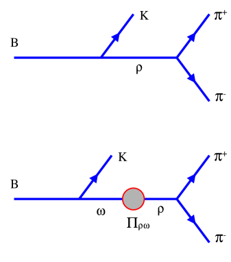
Figure 5: $B$ decays without (upper) and with (lower) $\rho-\omega$ mixing.

In order to obtain a large signal for direct $CP$ violation, we need some mechanism to make both $\sin\delta$ and $r$ large. We stress that $\rho-\omega$ mixing has the dual advantages that the strong phase difference is large (passing through $90^{o}$ at the $\omega$ resonance) and well known [4, 5]. With this mechanism (see Fig. 5), to first order in isospin violation, we have the following results when the invariant mass of $\pi^{+}\pi^{-}$ is near the $\omega$ resonance mass,

$$\langle K\pi^{-}\pi^{+}|H^{T}|B\rangle =\frac{g_{\rho}}{s_{\rho}s_{\omega}}\tilde{\Pi}_{\rho\omega}t_{\omega}+\frac{g_{\rho}}{s_{\rho}}t_{\rho}\ ,$$

$$\langle K\pi^{-}\pi^{+}|H^{P}|B\rangle =\frac{g_{\rho}}{s_{\rho}s_{\omega}}\tilde{\Pi}_{\rho\omega}p_{\omega}+\frac{g_{\rho}}{s_{\rho}}p_{\rho}\ .$$ (25)

Here $t_{V}\;(V=\rho\;{\rm or}\;\omega)$ is the tree amplitude and $p_{V}$ the penguin amplitude for producing a vector meson, $V$, $g_{\rho}$ is the coupling for $\rho^{0}\rightarrow\pi^{+}\pi^{-}$, $\tilde{\Pi}_{\rho\omega}$ is the effective $\rho-\omega$ mixing amplitude, and $s_{V}$ is from the inverse propagator of the vector meson $V$,

$$s_{V}=s-m_{V}^{2}+im_{V}\Gamma_{V}\ ,$$ (26)

with $\sqrt{s}$ being the invariant mass of the $\pi^{+}\pi^{-}$ pair. We stress that the direct coupling $\omega\rightarrow\pi^{+}\pi^{-}$ is effectively absorbed into $\tilde{\Pi}_{\rho\omega}$ [19], leading to the explicit $s$ dependence of $\tilde{\Pi}_{\rho\omega}$. Making the expansion $\tilde{\Pi}_{\rho\omega}(s)=\tilde{\Pi}_{\rho\omega}(m_{\omega}^{2})+(s-m_{w}^{2})\tilde{\Pi}_{\rho\omega}^{\prime}(m_{\omega}^{2})$, the $\rho-\omega$ mixing parameters were determined in the fit of Gardner and O’Connell [20]: $\Re e\;\tilde{\Pi}_{\rho\omega}(m_{\omega}^{2})=-3500\pm 300\;{\rm MeV}^{2},\;\;\;\Im m\;\tilde{\Pi}_{\rho\omega}(m_{\omega}^{2})=-300\pm 300\;{\rm MeV}^{2}$, and $\tilde{\Pi}_{\rho\omega}^{\prime}(m_{\omega}^{2})=0.03\pm 0.04$. In practice, the effect of the derivative term is negligible. ¿From Eqs. (22, 3.2) one has

$$re^{i\delta}e^{i\phi}=\frac{\tilde{\Pi}_{\rho\omega}p_{\omega}+s_{\omega}p_{\rho}}{\tilde{\Pi}_{\rho\omega}t_{\omega}+s_{\omega}t_{\rho}}\ .$$ (27)

Defining

$$\frac{p_{\omega}}{t_{\rho}}\equiv r^{\prime}e^{i(\delta_{q}+\phi)}\ ,\;\;\;\;\frac{t_{\omega}}{t_{\rho}}\equiv\alpha e^{i\delta_{\alpha}}\ ,\;\;\;\;\frac{p_{\rho}}{p_{\omega}}\equiv\beta e^{i\delta_{\beta}}\ ,$$ (28)

where $\delta_{\alpha},\delta_{\beta}$ and $\delta_{q}$ are strong phases (absorptive part). Substituting Eq. (28) into Eq. (27), one finds:

$$re^{i\delta}=r^{\prime}e^{i\delta_{q}}\frac{\tilde{\Pi}_{\rho\omega}+\beta e^{i\delta_{\beta}}s_{\omega}}{s_{\omega}+\tilde{\Pi}_{\rho\omega}\alpha e^{i\delta_{\alpha}}}\ ,$$ (29)

where

$$\alpha e^{i\delta_{\alpha}}=f,\;\;\;\beta e^{i\delta_{\beta}}=b+ci,\;\;\;r^{\prime}e^{i\delta_{q}}=d+ei\ ,$$ (30)

and using Eq. (29), we obtain the following result when $\sqrt{s}\sim m_{\omega}$:

$$re^{i\delta}=\frac{C+iD}{(s-m_{\omega}^{2}+f\Re e\;\tilde{\Pi}_{\rho\omega})^{2}+(f\Im m\;\tilde{\Pi}_{\rho\omega}+m_{\omega}\Gamma_{\omega})^{2}}\ .$$ (31)

Here $C$ and $D$ are defined as:

$$C=\bigl{(}s-m_{\omega}^{2}+f\Re e\;\tilde{\Pi}_{\rho\omega}\bigr{)}\Biggl{\{}d\biggl{[}\Re e\;\tilde{\Pi}_{\rho\omega}+b(s-m_{\omega}^{2})-cm_{\omega}\Gamma_{\omega}\biggr{]}\\ -e\biggl{[}\Im m\;\tilde{\Pi}_{\rho\omega}+bm_{\omega}\Gamma_{\omega}+c(s-m_{\omega}^{2})\biggr{]}\Biggr{\}}\\ +\bigl{(}f\Im m\;\tilde{\Pi}_{\rho\omega}+m_{\omega}\Gamma_{\omega}\bigr{)}\Biggl{\{}e\biggl{[}\Re e\;\tilde{\Pi}_{\rho\omega}+b(s-m_{\omega}^{2})-cm_{\omega}\Gamma_{\omega}\biggr{]}\\ +d\biggl{[}\Im m\;\tilde{\Pi}_{\rho\omega}+bm_{\omega}\Gamma_{\omega}+c(s-m_{\omega}^{2})\biggr{]}\Biggr{\}}\ ,$$ (32)

and

$$D=\bigl{(}s-m_{\omega}^{2}+f\Re e\;\tilde{\Pi}_{\rho\omega}\bigr{)}\Biggl{\{}e\biggl{[}\Re e\;\tilde{\Pi}_{\rho\omega}+d(s-m_{\omega}^{2})-cm_{\omega}\Gamma_{\omega}\biggr{]}\\ +d\biggl{[}\Im m\;\tilde{\Pi}_{\rho\omega}+bm_{\omega}\Gamma_{\omega}+c(s-m_{\omega}^{2})\biggr{]}\Biggr{\}}\\ -\bigl{(}f\Im m\;\tilde{\Pi}_{\rho\omega}+m_{\omega}\Gamma_{\omega}\bigr{)}\Biggl{\{}d\biggl{[}\Re e\;\tilde{\Pi}_{\rho\omega}+b(s-m_{\omega}^{2})-cm_{\omega}\Gamma_{\omega}\biggr{]}\\ -e\biggl{[}\Im m\;\tilde{\Pi}_{\rho\omega}+bm_{\omega}\Gamma_{\omega}+c(s-m_{\omega}^{2})\biggr{]}\Biggr{\}}\ .$$ (33)

$\alpha e^{i\delta_{\alpha}}$, $\beta e^{i\delta_{\beta}}$, and $r^{\prime}e^{i\delta_{q}}$ will be calculated later. In order to get the $CP$ violating asymmetry, $a$, $\sin\phi$ and $\cos\phi$ are needed, where $\phi$ is determined by the CKM matrix elements. In the Wolfenstein parametrization [15], the weak phase comes from $[V_{tb}V^{\star}_{ts}/V_{ub}V^{\star}_{us}]$ and one has for the decay $B\rightarrow\rho^{0}(\omega)K$,

$$\sin\phi =\frac{-\eta}{\sqrt{\rho^{2}+\eta^{2}}}\ ,$$

$$\cos\phi =\frac{-\rho}{\sqrt{\rho^{2}+\eta^{2}}}\ .$$ (34)

The values used for $\rho$ and $\eta$ will be discussed in Section 4.1.

3.3 Factorization

With the Hamiltonian given in Eq. (15) (see Section 2.3), we are ready to evaluate the matrix elements for $B^{\pm,0}\rightarrow\rho^{0}(\omega)K^{\pm,0}$. In the factorization approximation [21], either $\rho^{0}(\omega)$ or $K^{\pm,0}$ is generated by one current which has the appropriate quantum numbers in the Hamiltonian. For these decay processes, two kinds of matrix element products are involved after factorization (i.e. omitting Dirac matrices and color labels): $\langle\rho^{0}(\omega)|(\bar{u}u)|0\rangle\langle K^{\pm,0}|(\bar{s}b)|B^{\pm,0}\rangle$ and $\langle K^{\pm,0}|(\bar{q}_{1}q_{2})|0\rangle\langle\rho^{0}(\omega)|(\bar{u}b)|B^{\pm,0}\rangle$, where $q_{1}$ and $q_{2}$ could be $u,s$ or $d$. We will calculate them in several phenomenological quark models.
The matrix elements for $B\rightarrow X$ and $B\rightarrow X^{\star}$ (where X and $X^{\star}$ denote pseudoscalar and vector mesons, respectively) can be decomposed as follows [22],

$$\langle X|J_{\mu}|B\rangle=\left(p_{B}+p_{X}-\frac{m_{B}^{2}-m_{X}^{2}}{k^{2}}k\right)_{\mu}F_{1}(k^{2})+\frac{m_{B}^{2}-m_{X}^{2}}{k^{2}}k_{\mu}F_{0}(k^{2})\ ,$$ (35)

and,

$$\langle X^{\star}|J_{\mu}|B\rangle=\frac{2}{m_{B}+m_{X^{\star}}}\epsilon_{\mu\nu\rho\sigma}\epsilon^{\star\nu}p_{B}^{\rho}p_{X^{\star}}^{\sigma}V(k^{2})+i\Biggl{\{}\epsilon_{\mu}^{\star}(m_{B}+m_{X^{\star}})A_{1}(k^{2})\\ -\frac{\epsilon^{\star}\cdot k}{m_{B}+m_{X^{\star}}}(P_{B}+P_{X^{\star}})_{\mu}A_{2}(k^{2})-\frac{\epsilon^{\star}\cdot k}{k^{2}}2m_{X^{\star}}\cdot k_{\mu}A_{3}(k^{2})\Biggr{\}}\\ +i\frac{\epsilon^{\star}\cdot k}{k^{2}}2m_{X^{\star}}\cdot k_{\mu}A_{0}(k^{2})\ ,$$ (36)

where $J_{\mu}$ is the weak current, defined as $J_{\mu}=\bar{q}\gamma^{\mu}(1-\gamma_{5})b\;\;{\rm with}\;\;q=u,d,s$ and $k=p_{B}-p_{X(X^{\star})}$. $\epsilon_{\mu}$ is the polarization vector of $X^{\star}$. $F_{0}$ and $F_{1}$ are the form factors related to the transition $0^{-}\rightarrow 0^{-}$, while $A_{0},A_{1},A_{2},A_{3}$ and $V$ are the form factors that describe the transition $0^{-}\rightarrow 1^{-}$. Finally, in order to cancel the poles at $q^{2}=0$, the form factors respect the conditions:

$$F_{1}(0)=F_{0}(0),\;\;A_{3}(0)=A_{0}(0)\ ,$$ (37)

and they also satisfy the following relations:

$$A_{3}(k^{2})=\frac{m_{B}+m_{X^{\star}}}{2m_{X^{\star}}}A_{1}(k^{2})-\frac{m_{B}-m_{X^{\star}}}{2m_{X^{\star}}}A_{2}(k^{2})\ .$$ (38)

An argument for factorization has been given by Bjorken [23]: the heavy quark decays are very energetic, so the quark-antiquark pair in a meson in a final state moves very fast away from the localized weak interaction. The hadronization of the quark-antiquark pair occurs far away from the remaining quarks. Then, the meson can be factorized out and the interaction between the quark pair in the meson and the remaining quark should be tiny.

In the evaluation of matrix elements, the effective number of colors, $N_{c}^{eff}$, enters through a Fierz transformation. In general, for operator $O_{i}$, one can write,

$$\frac{1}{(N_{c}^{eff})_{i}}=\frac{1}{3}+\xi_{i}\ ,{\rm with}\;i=1,\cdots,10\ ,$$ (39)

where $\xi_{i}$ describes non-factorizable effects. We assume $\xi_{i}$ is universal for all the operators $O_{i}$. We also ignore the final state interactions (FSI). After factorization, and using the decomposition in Eqs. (35, 36), one obtains for the process ${\bar{B}}^{0}\rightarrow\rho^{0}(\omega){\bar{K}}^{0}$,

$$t_{\rho}=m_{B}|\vec{p}_{\rho}|\bigl{(}C_{1}^{\prime}+\frac{1}{N_{c}}C_{2}^{\prime}\bigr{)}f_{\rho}F_{1}(m_{\rho}^{2})\ ,$$ (40)

where $f_{\rho}$ is the $\rho$ decay constant (and to simplify the formulas we use $N_{c}$ for $N_{c}^{eff}$ in Eqs. (40)-(50)). In the same way, we find $t_{\omega}=t_{\rho}$, so that,

$$\alpha e^{i\delta_{\alpha}}=1\ .$$ (41)

After calculating the penguin operator contributions, one has,

$$r^{\prime}e^{i\delta_{q}}=-\frac{p_{\omega}}{(C_{1}^{\prime}+\frac{1}{N_{c}}C_{2}^{\prime})f_{\rho}F_{1}(m_{\rho}^{2})}\left|\frac{V_{tb}V_{ts}^{\star}}{V_{ub}V_{us}^{\star}}\right|\ ,$$ (42)

and

$$\beta e^{i\delta_{\beta}}=\frac{m_{B}|\vec{p}_{\rho}|}{p_{\omega}}\Bigg{\{}\frac{3}{2}\biggl{(}(C_{7}^{\prime}+\frac{1}{N_{c}}C_{8}^{\prime})+(C_{9}^{\prime}+\frac{1}{N_{c}}C_{10}^{\prime})\biggr{)}f_{\rho}F_{1}(m_{\rho}^{2})+\\ \hskip 40.00006pt\Biggl{(}(C_{4}^{\prime}+\frac{1}{N_{c}}C_{3}^{\prime})-\frac{1}{2}(C_{10}^{\prime}+\frac{1}{N_{c}}C_{9}^{\prime})\\ +\biggl{(}-2(C_{6}^{\prime}+\frac{1}{N_{c}}C_{5}^{\prime})+(C_{8}^{\prime}+\frac{1}{N_{c}}C_{7}^{\prime})\biggr{)}\left[\frac{m_{K}^{2}}{(m_{b}+m_{d})(m_{d}+m_{s})}\right]\Biggr{)}f_{K}A_{0}(m_{K}^{2})]\Bigg{\}}\ ,$$ (43)

where $f_{K}$ is the $K$ decay constant. In Eqs. (42, 43), $p_{\omega}$ has the following form:

$$p_{\omega}=m_{B}|\vec{p}_{\rho}|\Bigg{\{}2\biggl{(}(C_{3}^{\prime}+\frac{1}{N_{c}}C_{4}^{\prime})+(C_{5}^{\prime}+\frac{1}{N_{c}}C_{6}^{\prime})\biggr{)}f_{\rho}F_{1}(m_{\rho}^{2})\\ \hskip 55.00008pt+\frac{1}{2}\biggl{(}(C_{7}^{\prime}+\frac{1}{N_{c}}C_{8}^{\prime})+(C_{9}^{\prime}+\frac{1}{N_{c}}C_{10}^{\prime})\biggr{)}f_{\rho}F_{1}(m_{\rho}^{2})\\ +\biggl{(}(C_{8}^{\prime}+\frac{1}{N_{c}}C_{7}^{\prime})-2(C_{6}^{\prime}+\frac{1}{N_{c}}C_{5}^{\prime})\biggl{)}\left[\frac{m_{K}^{2}f_{K}A_{0}(m_{K}^{2})}{(m_{b}+m_{d})(m_{d}+m_{s})}\right]\\ +\biggl{(}(C_{4}^{\prime}+\frac{1}{N_{c}}C_{3}^{\prime})-\frac{1}{2}(C_{10}^{\prime}+\frac{1}{N_{c}}C_{9}^{\prime})\biggr{)}f_{K}A_{0}(m_{K}^{2})\Bigg{\}}\ ,$$ (44)

and the CKM amplitude entering the $b\rightarrow s$ transition is,

$$\left|\frac{V_{tb}V_{ts}^{\star}}{V_{ub}V_{us}^{\star}}\right|=\frac{1}{\lambda^{2}}\frac{1}{\sqrt{{\rho}^{2}+{\eta}^{2}}}=\frac{1}{\lambda^{2}}\frac{1}{|\sin\beta|}\ ,$$ (45)

with $\beta$ defined as the unitarity triangle as usual. Similarly, by applying the same formalism, one gets for the decay $B^{-}\rightarrow\rho^{0}(\omega)K^{-}$,

$$t_{\rho}=m_{B}|\vec{p}_{\rho}|\left[(C_{1}^{\prime}+\frac{1}{N_{c}}C_{2}^{\prime})f_{\rho}F_{1}(m_{\rho}^{2})+(C_{2}^{\prime}+\frac{1}{N_{c}}C_{1}^{\prime})f_{K}A_{0}(m_{K}^{2})\right]\ .$$ (46)

In the same way, we find $t_{\omega}=t_{\rho}$, therefore one has again,

$$\alpha e^{i\delta_{\alpha}}=1\ .$$ (47)

The ratio between penguin and tree operator contributions, which involves CKM matrix elements, is given by,

$$r^{\prime}e^{i\delta_{q}}=-\frac{p_{\omega}}{(C_{1}^{\prime}+\frac{1}{N_{c}}C_{2}^{\prime})f_{\rho}F_{1}(m_{\rho}^{2})+(C_{2}^{\prime}+\frac{1}{N_{c}}C_{1}^{\prime})f_{K}A_{0}(m_{K}^{2})}\left|\frac{V_{tb}V_{ts}^{\star}}{V_{ub}V_{us}^{\star}}\right|\ ,$$ (48)

and finally,

$$\beta e^{i\delta_{\beta}}=\frac{m_{B}|\vec{p}_{\rho}|}{p_{\omega}}\Bigg{\{}(C_{4}^{\prime}+\frac{1}{N_{c}}C_{3}^{\prime})f_{K}A_{0}(m_{K}^{2})\\ +\frac{3}{2}\biggl{(}(C_{7}^{\prime}+\frac{1}{N_{c}}C_{8}^{\prime})+(C_{9}^{\prime}+\frac{1}{N_{c}}C_{10}^{\prime})\biggr{)}f_{\rho}F_{1}(m_{\rho}^{2})+(C_{10}^{\prime}+\frac{1}{N_{c}}C_{9}^{\prime})f_{K}A_{0}(m_{K}^{2})\\ -2\biggl{(}(C_{6}^{\prime}+\frac{1}{N_{c}}C_{5}^{\prime})+(C_{8}^{\prime}+\frac{1}{N_{c}}C_{7}^{\prime})\biggr{)}\left[\frac{m_{K}^{2}f_{K}A_{0}(m_{K}^{2})}{(m_{u}+m_{s})(m_{b}+m_{u})}\right]\Bigg{\}}\ ,$$ (49)

where the $\omega$ penguin contribution, $p_{\omega}$, is:

$$p_{\omega}=m_{B}|\vec{p}_{\rho}|\Bigg{\{}2\biggl{(}(C_{3}^{\prime}+\frac{1}{N_{c}}C_{4}^{\prime})+(C_{5}^{\prime}+\frac{1}{N_{c}}C_{6}^{\prime})\biggr{)}f_{\rho}F_{1}(m_{\rho}^{2})\\ +\frac{1}{2}\biggl{(}(C_{7}^{\prime}+\frac{1}{N_{c}}C_{8}^{\prime})+(C_{9}^{\prime}+\frac{1}{N_{c}}C_{10}^{\prime})\biggr{)}f_{\rho}F_{1}(m_{\rho}^{2})+\biggl{(}(C_{4}^{\prime}+\frac{1}{N_{c}}C_{3}^{\prime})+(C_{10}^{\prime}+\frac{1}{N_{c}}C_{9}^{\prime})\biggr{)}f_{K}A_{0}(m_{K}^{2})\\ -2\biggl{(}(C_{8}^{\prime}+\frac{1}{N_{c}}C_{7}^{\prime})+(C_{6}^{\prime}+\frac{1}{N_{c}}C_{5}^{\prime})\biggr{)}\left[\frac{m_{K}^{2}}{(m_{u}+m_{s})(m_{b}+m_{u})}\right]f_{K}A_{0}(m_{K}^{2})\Bigg{\}}\ .$$ (50)

3.4 Form factors

The form factors $F_{i}(k^{2})$ and $A_{j}(k^{2})$ depend on the inner structure of the hadrons. We will adopt here three different theoretical approaches. The first was proposed by Bauer, Stech, and Wirbel [22] (BSW), who used the overlap integrals of wave functions in order to evaluate the meson-meson matrix elements of the corresponding current. The momentum dependence of the form factors is based on a single-pole ansatz. The second one was developed by Guo and Huang (GH) [24]. They modified the BSW model by using some wave functions described in the light-cone framework. The last model was given by Ball [25] and Ball and Braun [26]. In this case, the form factors are calculated from QCD sum rules on the light-cone and leading twist contributions, radiative corrections, and $SU(3)$-breaking effects are included. Nevertheless, all these models use phenomenological form factors which are parametrized by making the nearest pole dominance assumption. The explicit $k^{2}$ dependence of the form factor is as [22, 24, 25, 26, 27]:

$$F_{1}(k^{2})=\frac{h_{1}}{\left(1-\frac{k^{2}}{m_{1}^{2}}\right)^{n}}\ ,\;\;\;\;\;\;A_{0}(k^{2})=\frac{h_{A_{0}}}{\left(1-\frac{k^{2}}{m_{A_{0}}^{2}}\right)^{n}}\ ,$$

$${\rm or}\hskip 378.0006pt$$

$$F_{1}(k^{2})=\frac{h_{1}}{1-d_{1}\frac{k^{2}}{m_{B}^{2}}+b_{1}\left(\frac{k^{2}}{m_{B}^{2}}\right)^{2}}\ ,\;\;\;\;\;\;A_{0}(k^{2})=\frac{h_{A_{0}}}{1-d_{0}\frac{k^{2}}{m_{B}^{2}}+b_{0}\left(\frac{k^{2}}{m_{B}^{2}}\right)^{2}}\ ,$$ (51)

where $n=1,2$, $m_{A_{0}}$ and $m_{1}$ are the pole masses associated with the transition current, $h_{1}$ and $h_{A_{0}}$ are the values of form factors at $q^{2}=0$, and $d_{i}$ and $b_{i}$ ($i=0,1$) are parameters in the model of Ball.

4 Numerical inputs

4.1 CKM values

In our numerical calculations we have several parameters: $q^{2},N_{c}^{eff}$, and the CKM matrix elements in the Wolfenstein parametrization. As mentioned in Section 2.2, the value of $q^{2}$ is conventionally chosen to be in the range $0.3<q^{2}/{m_{b}}^{2}<0.5$. The CKM matrix, which should be determined from experimental data, is expressed in terms of the Wolfenstein parameters, $A,\;\lambda,\;\rho$, and $\eta$ [15]. Here, we shall use the latest values [28] which were extracted from charmless semileptonic $B$ decays, ($|V_{ub}|$), charm semileptonic $B$ decays, ($|V_{cb}|$), $s$ and $d$ mass oscillations, $\Delta m_{s},\Delta m_{d}$, and $CP$ violation in the kaon system ($\epsilon_{K}$), ($\rho,\eta$). Hence, one has,

$$\lambda=0.2237\ ,\;\;A=0.8113\ ,\;\;0.190<\rho<0.268\ ,\;\;0.284<\eta<0.366\ .$$ (52)

These values respect the unitarity triangle as well (see also Table 3).

4.2 Quark masses

The running quark masses are used in order to calculate the matrix elements of penguin operators. The quark mass is taken at the scale $\mu\simeq m_{b}$ in $B$ decays. Therefore one has [29],

$$m_{u}(\mu=m_{b}) =2.3\;{\rm MeV}\ , m_{d}(\mu=m_{b}) =4.6\;{\rm MeV}\ ,$$

$$m_{s}(\mu=m_{b}) =90\;{\rm MeV}\ , m_{b}(\mu=m_{b}) =4.9\;{\rm GeV}\ ,$$ (53)

which corresponds to $m_{s}(\mu=1\;{\rm GeV})=140\;{\rm MeV}$. For meson masses, we shall use the following values [18]:

$$m_{B^{\pm}} =5.279\;{\rm GeV}\ , m_{B^{0}} =5.279\;{\rm GeV}\ ,$$

$$m_{K^{\pm}} =0.493\;{\rm GeV}\ , m_{K^{0}} =0.497\;{\rm GeV}\ ,$$

$$m_{\pi^{\pm}} =0.139\;{\rm GeV}\ , m_{\pi^{0}} =0.135\;{\rm GeV}\ ,$$

$$m_{\rho^{0}} =0.769\;{\rm GeV}\ , m_{\omega} =0.782\;{\rm GeV}\ .$$ (54)

4.3 Form factors and decay constants

In Table 4 we list the relevant form factor values at zero momentum transfer [22, 24, 25, 26, 30] for the $B\rightarrow K$ and $B\rightarrow\rho$ transitions. The different models are defined as follows: models (1) and (3) are the BSW model where the $q^{2}$ dependence of the form factors is described by a single- and a double-pole ansatz, respectively. Models (2) and (4) are the GH model with the same momentum dependence as models (1) and (3). Finally, model (5) refers to the Ball model. We define the decay constants for pseudo-scalar ($f_{P}$) and vector ($f_{V}$) mesons as usual by,

$$\langle P(q)|\bar{q}_{1}\gamma_{\mu}\gamma_{5}q_{2}|0\rangle =if_{P}q_{\mu}\ ,$$

$$\sqrt{2}\langle V(q)|\bar{q}_{1}\gamma_{\mu}q_{2}|0\rangle =f_{V}m_{V}\epsilon_{V}\ ,$$ (55)

with $q_{\mu}$ being the momentum of the pseudo-scalar meson, $m_{V}$ and $\epsilon_{V}$ being the mass and polarization vector of the vector meson, respectively. Numerically, in our calculations, we take [18],

$$f_{K}=160\;{\rm MeV}\ ,\;f_{\rho}\simeq f_{\omega}=221\;{\rm MeV}\ .$$ (56)

The $\rho$ and $\omega$ decay constants are very close and for simplification (without any consequences for results) we choose $f_{\rho}=f_{\omega}$.

5 Results and discussion

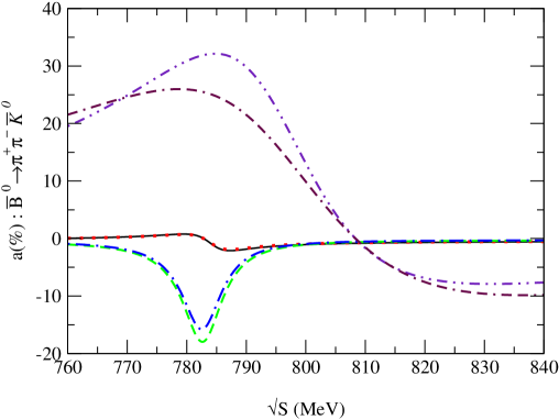
Figure 6: $CP$ violating asymmetry, $a$, for ${\bar{B}}^{0}\rightarrow\pi^{+}\pi^{-}{\bar{K}}^{0}$, for $k^{2}/m_{b}^{2}=0.3$, for $N_{c}^{eff}=0.66,2.69,2.84$ and for limiting values, max (min), of the CKM matrix elements for model $(1)$: dot-dot-dashed line (dot-dash-dashed line) for $N_{c}^{eff}=0.66$. Solid line (dotted line) for $N_{c}^{eff}=2.69$. Dashed line (dot-dashed line) for $N_{c}^{eff}=2.84$.

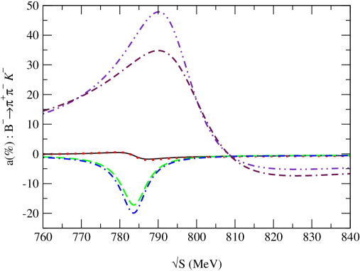
Figure 8: $CP$ violating asymmetry, $a$, for $B^{-}\rightarrow\pi^{+}\pi^{-}K^{-}$, for $k^{2}/m_{b}^{2}=0.3$, for $N_{c}^{eff}=0.66,2.69,2.84$ and for limiting values, max (min), of the CKM matrix elements for model $(1)$: dot-dot-dashed line (dot-dash-dashed line) for $N_{c}^{eff}=0.66$. Solid line (dotted line) for $N_{c}^{eff}=2.69$. Dashed line (dot-dashed line) for $N_{c}^{eff}=2.84$.

We have investigated the $CP$ violating asymmetry, $a$, for the two $B$ decays: ${\bar{B}}^{0}\rightarrow\rho^{0}{\bar{K}}^{0}\rightarrow\pi^{+}\pi^{-}{\bar{K}}^{0}$ and $B^{-}\rightarrow\rho^{0}K^{-}\rightarrow\pi^{+}\pi^{-}K^{-}$. The results are shown in Figs. 6 and 7 for ${\bar{B}}^{0}\rightarrow\pi^{+}\pi^{-}{\bar{K}}^{0}$, ($a=[\Gamma({\bar{B}}^{0}\rightarrow\pi^{+}\pi^{-}{\bar{K}}^{0})-\Gamma(B^{0}\rightarrow\pi^{-}\pi^{+}K^{0})]/[\Gamma({\bar{B}}^{0}\rightarrow\pi^{+}\pi^{-}{\bar{K}}^{0})+\Gamma(B^{0}\rightarrow\pi^{-}\pi^{+}K^{0})]$), where $k^{2}/m_{b}^{2}=0.3(0.5)$ and for $N_{c}^{eff}$ equal to $0.61,0.66,2.65,2.69,2.82$ and $2.84$. Similarly, in Figs. 8 and 9, the $CP$ violating asymmetry, $a$, ($=[\Gamma(B^{-}\rightarrow\pi^{+}\pi^{-}K^{-})-\Gamma(B^{+}\rightarrow\pi^{-}\pi^{+}K^{+})]/[\Gamma(B^{-}\rightarrow\pi^{+}\pi^{-}K^{-})+\Gamma(B^{+}\rightarrow\pi^{-}\pi^{+}K^{+})]$), is plotted for $B^{-}\rightarrow\pi^{+}\pi^{-}K^{-}$, where $k^{2}/m_{b}^{2}=0.3(0.5)$ and for the same values of $N_{c}^{eff}$ previously applied for ${\bar{B}}^{0}\rightarrow\pi^{+}\pi^{-}{\bar{K}}^{0}$. In our numerical calculations, we found that the $CP$ violating parameter, $a$, reaches a maximum value, $a_{max}$, when the invariant mass of the $\pi^{+}\pi^{-}$ is in the vicinity of the $\omega$ resonance, for a fixed value of $N_{c}^{eff}$. We have studied the model dependence of $a$ with five models where different form factors have been applied. Numerical results for ${\bar{B}}^{0}\rightarrow\pi^{+}\pi^{-}{\bar{K}}^{0}$ and $B^{-}\rightarrow\pi^{+}\pi^{-}K^{-}$ are listed in Tables 5 and 6, respectively. It appears that the form factor dependence of $a$ for all models, and in both decays, is weaker than the $N_{c}^{eff}$ dependence.

For ${\bar{B}}^{0}\rightarrow\pi^{+}\pi^{-}{\bar{K}}^{0}$, we have determined the range of the maximum asymmetry parameter, $a_{max}$, when $N_{c}^{eff}$ varies between $0.66(0.61)$ and $2.84(2.82)$, in the case of $k^{2}/m_{b}^{2}=0.3(0.5)$. The evaluation of $a_{max}$ gives allowed values from $37\%(55\%)$ to $-20\%(-24\%)$ for the range of $N_{c}^{eff}$ and CKM matrix elements indicated before. The sign of $a_{max}$ stays positive until $N_{c}^{eff}$ reaches $2.7$. If we look at the numerical results for the asymmetries (Table 5), for $N_{cmin}^{eff}=0.66(0.61)$ and $k^{2}/m_{b}^{2}=0.3(0.5)$, we find good agreement between all the models, with a maximum asymmetry, $a_{max}$, around $33\%(45.6\%)$ for the set $(\rho_{max},\eta_{max})$, and around $26\%(33.2\%)$ for the set $(\rho_{min},\eta_{min})$. The ratio between asymmetries associated with the upper and lower limits of $(\rho,\eta)$ is around $1.26(1.37)$. If we consider the maximum asymmetry parameter, $a_{max}$, for $N_{cmax}^{eff}=2.84(2.82)$, we observe a distinction between the models. Indeed, two classes of models appear: models $(2)$ and $(4)$ and models $(1,3)$ and $(5)$. For models $(2)$ and $(4)$, one has an asymmetry, $a_{max}$, around $-6\%(-7\%)$ and around $-9\%(-10\%)$ for the upper and lower set of $(\rho,\eta)$, respectively. The ratio between them is around $1.50(1.42)$. For models $(1,3)$ and $(5)$, the maximum asymmetry is of order $-14.3\%(-16.3\%)$ for $(\rho_{max},\eta_{max})$ and around $-19.3\%(-23.0\%)$ for $(\rho_{min},\eta_{min})$. In this case, the ratio between asymmetries is around $1.34(1.41)$.

The first reason why the maximum asymmetry, $a_{max}$, can vary so much comes from the element $V_{ub}$. The other CKM matrix elements $V_{tb},V_{ts}$ and $V_{us}$, all proportional to $A$ and $\lambda$, are very well measured experimentally and thus do not interfere in our results. Only $V_{ub}$, which contains the $\rho$ and $\eta$ parameters, provides large uncertainties, and thus, large variations for the maximum asymmetry. The second reason is the non-factorizable effects in the transition $b\rightarrow s$. It is well known that decays including a $K$ meson (and therefore an $s$ quark) carry more uncertainties than those involving only a $\pi$ meson ($u$,$d$ quarks). If we look at the asymmetries at $N_{cmin}^{eff}$, all models give almost the same values, whereas at $N_{cmax}^{eff}$, we obtain different asymmetry values (with, moreover, a change of sign for the $CP$ violating asymmetry). The $CP$ asymmetry parameter is more sensitive to form factors at high values of $N_{c}^{eff}$ than at low values of $N_{c}^{eff}$. It appears therefore that all of the models investigated can be divided in two classes, referring to the two classes of form factors.

For $B^{-}\rightarrow\pi^{+}\pi^{-}K^{-}$, we have similarly investigated the $CP$ violating asymmetry. The values of maximum asymmetry parameter, $a_{max}$, for a range of $N_{c}^{eff}$ from $0.66(0.61)$ to $2.84(2.82)$, where $k^{2}/m_{b}^{2}=0.3(0.5)$ and for the five models analyzed, are given in Table 6. We found that for this decay, the $CP$ violating parameter, $a$, takes values around $49\%(46\%)$ to $-22\%(-25\%)$ for the limiting CKM matrix values of $\rho$ and $\eta$ defined before. Once again, the sign of the asymmetry parameter, $a$, is positive if the value of $N_{c}^{eff}$ stays below $2.7$. If we focus on $N_{cmin}^{eff}$ equal to $0.66(0.61)$, models $(1,2,3,4)$ and $(5)$ give almost the same value which is around $46.6\%(43.6\%)$ for the maximum values of the CKM matrix elements. For the set $(\rho_{min},\eta_{min})$, the maximum asymmetry, $a$, is around $34.0\%(33.8\%)$. The ratio between asymmetry values taken at upper and lower limiting $\rho$ and $\eta$ values is around $1.37(1.28)$. Let us have a look at the $CP$ asymmetry values at $N_{cmax}^{eff}$. As we observed for the decay ${\bar{B}}^{0}\rightarrow\pi^{+}\pi^{-}{\bar{K}}^{0}$, all models are separated into two distinct classes related to their form factors. For models $(1,3)$ and $(5)$, the value of maximum asymmetry, $a_{max}$, is around $-15.6\%(-17.6\%)$ and around $-21\%(-23.6\%)$ for the maximum and minimum values of set $(\rho,\eta)$, respectively. The calculated ratio is around $1.34(1.34)$, between these two asymmetries. As regards models $(2)$ and $(4)$, for the same set of $(\rho,\eta)$, one gets $-11.5\%(-13\%)$ and $-17\%(-18\%)$. In this case, one has $1.47(1.38)$ for the ratio. The reasons for the differences between the maximum asymmetry parameter, $a_{max}$, are the same as in the decay ${\bar{B}}^{0}\rightarrow\pi^{+}\pi^{-}{\bar{K}}^{0}$.

By analyzing the $B$ decays, such as ${\bar{B}}^{0}\rightarrow\pi^{+}\pi^{-}{\bar{K}}^{0}$ and $B^{-}\rightarrow\pi^{+}\pi^{-}K^{-}$, we found that the $CP$ violating asymmetry, $a$, depends on the CKM matrix elements, form factors and the effective parameter $N_{c}^{eff}$ (in order of increasing dependence). As regards the CKM matrix elements, the dependence through the element, $V_{ub}$, contributes to the asymmetry in the ratio between the $\omega$ penguin contributions and the $\rho$ tree contributions. It also appears that for the upper limit of set $(\rho,\eta)$, we get the higher value asymmetry, $a$, and vice versa. With regard to the form factors, the dependence at low values of $N_{c}^{eff}$ is very weak although the huge difference between the phenomenological form factors (models $(2)$ and $(4)$ and models $(1,3)$ and $(5)$) applied in our calculations. At high values of $N_{c}^{eff}$, the dependence becomes strong and then, the asymmetry appears very sensitive to form factors. For the effective parameter, $N_{c}^{eff}$, (related to hadronic non-factorizable effects), our results show explicitly the dependence of the asymmetry parameter on it. Because of the energy carried by the quark $s$, intermediate states and final state interactions are not well taken into account and may explain this strong sensitivity. Finally, results obtained at $k^{2}/m_{b}^{2}=0.3(0.5)$, also show renormalization effects of the Wilson coefficients involved in the weak effective hadronic Hamiltonian. For the ratio between asymmetries, results give an average value of order $1.36(1.40)$ for ${\bar{B}}^{0}\rightarrow\pi^{+}\pi^{-}{\bar{K}}^{0}$ and $1.39(1.33)$ for $B^{-}\rightarrow\pi^{+}\pi^{-}K^{-}$. This ratio is mainly governed by the term $1/\sin\beta$, where the values of the angles $\alpha,\beta$ and $\gamma$ are listed in Table 3.

As a first conclusion on these numerical results, it is obvious that the dependence of the asymmetry on the effective parameter $N_{c}^{eff}$ is dramatic and therefore it is absolutely necessary to more efficiently constrain its value, in order to use asymmetry, $a$, to determine the CKM parameters $\rho$ and $\eta$. We know that the effects of $\rho-\omega$ mixing only exist around $\omega$ resonance. Nevertheless, in Figs. 6, 7, 8, and 9, at small values of $N_{c}^{eff}$, e.g. $\simeq 0.6$, the curves show large asymmetry values far away from $\omega$ resonance, which is a priori unexpected. In fact, if we assume that nonfactorizable effects are not as important as factorizable contributions, then $N_{c}^{eff}$ should be much bigger (see Eq. (39)). ¿From previous analysis on some other $B$ decays such as $B\rightarrow D\pi,B\rightarrow\omega\pi$, and $B\rightarrow\omega K$, it was found that $N_{c}^{eff}$ should be around $2$ [31]. Therefore, although small values of $N_{c}^{eff}$ are allowed by the experimental data we are considering in this paper, we expect that the value of $N_{c}^{eff}$ cannot be so small with more accurate data. We have checked that when $N_{c}^{eff}$ is larger than $1$ the large $CP$ asymmetries are confined in the $\omega$ resonance region. With a very small value of $N_{c}^{eff}$, nonfactorizable effects have been overestimated. This means that soft gluon exchanges between $\rho^{0}(\omega)$ and $K$ may affect $\rho-\omega$ mixing and hence lead to the large $CP$ asymmetries in a region far away from $\omega$ resonance. However, when $\sqrt{s}$ is very far from $\omega$ resonance, the $CP$ asymmetries go to zero as expected.

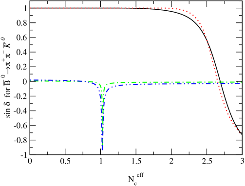
Figure 10: $\sin\delta$, as a function of $N_{c}^{eff}$, for ${\bar{B}}^{0}\rightarrow\pi^{+}\pi^{-}{\bar{K}}^{0}$, for $k^{2}/m_{B}^{2}=0.3(0.5)$ and for model $(1)$. The solid (dotted) line at $\sin\delta=+1$ corresponds to the case $\tilde{\Pi}_{\rho\omega}=(-3500;-300)$, where $\rho-\omega$ mixing is included. The dot-dashed (dot-dot-dashed) line corresponds to $\tilde{\Pi}_{\rho\omega}=(0;0)$, where $\rho-\omega$ mixing is not included.

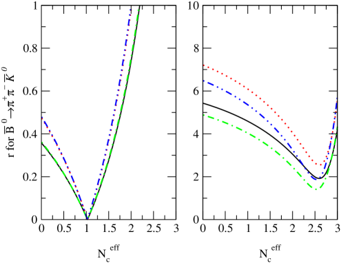
Figure 12: The ratio of penguin to tree amplitudes, $r$, as a function of $N_{c}^{eff}$, for ${\bar{B}}^{0}\rightarrow\pi^{+}\pi^{-}{\bar{K}}^{0}$, for $k^{2}/m_{B}^{2}=0.3(0.5)$, for limiting values of the CKM matrix elements $(\rho,\eta)$ max(min), for $\tilde{\Pi}_{\rho\omega}=(-3500;-300)(0,0)$, (i.e. with(without) $\rho-\omega$ mixing) and for model $(1)$. Figure 12a (left): for $\tilde{\Pi}_{\rho\omega}=(0;0)$, solid line (dotted line) for $k^{2}/m_{B}^{2}=0.3$ and $(\rho,\eta)$ max(min). Dot-dashed line (dot-dot-dashed line) for $k^{2}/m_{B}^{2}=0.5$ and $(\rho,\eta)$ max(min). Figure 12b (right): same caption but for $\tilde{\Pi}_{\rho\omega}=(-3500;-300)$.

In spite of the uncertainties discussed previously, the main effect of $\rho-\omega$ mixing in $B\rightarrow\pi^{+}\pi^{-}K$ is the removal of the ambiguity concerning the strong phase, $\sin\delta$. In the $b\rightarrow s$ transition, the weak phase in the rate asymmetry is proportional to $\sin\gamma$ where $\gamma=arg[-(V_{ts}V_{tb}^{\star})/(V_{us}V_{ub}^{\star})]$. Knowing the sign of $\sin\delta$, we are then able to determine the sign of $\sin\gamma$ from a measurement of the asymmetry, $a$. In Figs. 10 and 11, the value of $\sin\delta$ is plotted as a function of $N_{c}^{eff}$ for ${\bar{B}}^{0}\rightarrow\pi^{+}\pi^{-}{\bar{K}}^{0}$ and $B^{-}\rightarrow\pi^{+}\pi^{-}K^{-}$, respectively. It appears, in both cases, when $\rho-\omega$ mixing mechanism is included, that the sign of $\sin\delta$ is positive, for all models studied, until $N_{c}^{eff}$ reaches $2.69(2.65)$ for both $B^{-}\rightarrow\pi^{+}\pi^{-}K^{-}$ and ${\bar{B}}^{0}\rightarrow\pi^{+}\pi^{-}{\bar{K}}^{0}$, when $k^{2}/m_{b}^{2}=0.3(0.5)$. For values of $N_{c}^{eff}$ bigger than this limit, $\sin\delta$ becomes negative. At the same time, the sign of the asymmetry also changes. In Figs. 12b and 13b, the ratio of penguin to tree amplitudes is shown for $B^{\pm,0}\rightarrow\pi^{+}\pi^{-}K^{\pm,0}$, in the case of $\tilde{\Pi}_{\rho\omega}=(-3500,-300)$. The critical point around $N_{c}^{eff}=2.7$, refers to the change of sign of $\sin\delta$. Clearly, we can use a measurement of the asymmetry, $a$, to eliminate the uncertainty mod$(\pi)$ which is usually involved in the determination of $\gamma$ (through $\sin 2\gamma$). If we do not take into account $\rho-\omega$ mixing, the $CP$ violating asymmetry, $a$, remains very small (just a few percent) in both decays. In Figs. 10 and 11 (for the evolution of $\sin\delta$) and in Figs. 12a and 13a (for the evolution of penguin to tree amplitudes), for $B^{\pm,0}\rightarrow\pi^{+}\pi^{-}K^{\pm,0}$, we plot $\sin\delta$ and $r$ when $\tilde{\Pi}_{\rho\omega}=(0,0)$ –i.e. without $\rho-\omega$ mixing. There is a critical point at $N_{c}^{eff}=1$ (for ${\bar{B}}^{0}\rightarrow\pi^{+}\pi^{-}{\bar{K}}^{0}$) and $N_{c}^{eff}=0.24$ (for $B^{-}\rightarrow\pi^{+}\pi^{-}K^{-}$) for which the value of $\sin\delta$ is at its maximum and corresponds (for the same value of $N_{c}^{eff}$), to the lowest value of $r$. The last results show the double effect of the $\rho-\omega$ mixing: the $CP$ violating asymmetry increases and the sign of the strong phase $\delta$ is determined.

6 Branching ratios for $B^{\pm,0}\rightarrow\rho^{0}K^{\pm,0}$

6.1 Formalism

With the factorized decay amplitudes, we can compute the decay rates by using the following expression [27],

$$\Gamma(B\rightarrow VP)=\frac{|\vec{p}_{\rho}|^{3}}{8\pi m_{V}^{2}}\left|\frac{A(B\rightarrow VP)}{\epsilon_{V}\cdot p_{B}}\right|^{2}\ ,$$ (57)

where $\vec{p}_{\rho}$ is the c.m. momentum of the decay particles defined as,

$$|\vec{p}_{\rho}|=\frac{\sqrt{[m_{B}^{2}-(m_{1}+m_{2})^{2}][m_{B}^{2}-(m_{1}-m_{2})^{2}]}}{2m_{B}}\ .$$ (58)

$m_{1}(m_{2})$ is the mass of the vector (pseudo-scalar) $V(P)$ particle, $\epsilon_{V}$ is the polarization vector and $A(B\rightarrow VP)$ is the decay amplitude given by,

$$A(B\rightarrow VP)=\frac{G_{F}}{\sqrt{2}}\sum_{i=1,10}V_{s}^{T,P}a_{i}\langle VP|O_{i}|B\rangle\ ,$$ (59)

where the effective parameters, $a_{i}$, which are involved in the decay amplitude, are the following combinations of effective Wilson coefficients:

$$a_{2j}=C_{2j}^{\prime}+\frac{1}{N_{c}^{eff}}C_{2j-1}^{\prime},\;\;\;a_{2j-1}=C_{2j-1}^{\prime}+\frac{1}{N_{c}^{eff}}C_{2j}^{\prime},\;\;{\rm for}\;\;j=1,\cdots,5\ .$$ (60)

All other variables in Eq. (59) have been introduced earlier. In the Quark Model, the diagram (Fig. 5 top) gives the main contribution to the $B\rightarrow\rho^{0}K$ decay. In our case, to be consistent, we should also take into account the $\rho-\omega$ mixing contribution (Fig. 5 bottom) when we calculate the branching ratio, since we are working to the first order of isospin violation. The application is straightforward and we obtain the branching ratio for $B\rightarrow\rho^{0}K$:

$${\rm BR}(B\rightarrow\rho^{0}K)=\frac{G_{F}^{2}|\vec{p}_{\rho}|^{3}}{\alpha_{k}\pi\Gamma_{B}}\Bigg{|}\bigg{[}V_{s}^{T}A^{T}_{\rho^{0}}(a_{1},a_{2})-V_{s}^{P}A^{P}_{\rho^{0}}(a_{3},\cdots,a_{10})\bigg{]}\\ +\bigg{[}V_{s}^{T}A^{T}_{\omega}(a_{1},a_{2})-V_{s}^{P}A^{P}_{\omega}(a_{3},\cdots,a_{10})\bigg{]}\frac{\tilde{\Pi}_{\rho\omega}}{(s_{\rho}-m_{\omega}^{2})+im_{\omega}\Gamma_{\omega}}\Bigg{|}^{2}\ .$$ (61)

In Eq. (61) $G_{F}$ is the Fermi constant, $\Gamma_{B}$ is the total width $B$ decay, and $\alpha_{k}$ is an integer related to the given decay. $A^{T}_{V}$ and $A^{P}_{V}$ are the tree and penguin amplitudes which respect quark interactions in the $B$ decay. $V_{s}^{T,P}$ (in Eq. (59)) or $V_{s}^{T},V_{s}^{P}$ (in Eq. (61)) represent the CKM matrix elements involved in the tree and penguin diagram, respectively:

$$V_{s}^{T}=|V_{ub}V_{us}^{\star}|\;\;{\rm for}\;\;\;\;i=1,2\ ,\;\;\;\;{\rm and}\;\;\;V_{s}^{P}=|V_{tb}V_{ts}^{\star}|\;\;{\rm for}\;\;\;\;i=3,\cdots,10\ .$$ (62)

6.2 Calculational details

In this section, we enumerate the theoretical decay amplitudes. We shall analyze five $b$ into $s$ transitions. Two of them involve $\rho-\omega$ mixing. These are $B^{-}\rightarrow\rho^{0}K^{-}$ and ${\bar{B}}^{0}\rightarrow\rho^{0}{\bar{K}}^{0}$. Two other decays are ${\bar{B}}^{0}\rightarrow\rho^{-}K^{+}$ and $B^{-}\rightarrow\rho^{-}{\bar{K}}^{0}$ and the last one is $B^{-}\rightarrow\omega K^{-}$. We list in the following, the tree and penguin amplitudes which appear in the given transitions.
For the decay $B^{-}\rightarrow\rho^{0}K^{-}$ ($\alpha_{k}=32$ in Eq. (61)),

$$\sqrt{2}A^{T}_{\rho}(a_{1},a_{2})=a_{1}f_{\rho}F_{1}(m_{\rho}^{2})+a_{2}f_{K}A_{0}(m_{K}^{2})\ ,\hskip 160.00024pt$$ (63)

$$\sqrt{2}A^{P}_{\rho}(a_{3},\cdots,a_{10})=f_{\rho}F_{1}(m_{\rho}^{2})\biggl{\{}\frac{3}{2}(a_{7}+a_{9})\biggr{\}}\\ +f_{K}A_{0}(m_{K}^{2})\Biggl{\{}a_{4}+a_{10}-2(a_{6}+a_{8})\biggl{[}\frac{m_{K}^{2}}{(m_{u}+m_{s})(m_{b}+m_{u})}\biggr{]}\Biggl{\}}\ ;$$ (64)

for the decay $B^{-}\rightarrow\omega K^{-}$ ($\alpha_{k}=32$ in Eq. (61)),

$$\sqrt{2}A^{T}_{\omega}(a_{1},a_{2})=a_{1}f_{\rho}F_{1}(m_{\rho}^{2})+a_{2}f_{K}A_{0}(m_{K}^{2})\ ,\hskip 160.00024pt$$ (65)

$$\sqrt{2}A^{P}_{\omega}(a_{3},\cdots,a_{10})=f_{\rho}F_{1}(m_{\rho}^{2})\bigg{\{}2(a_{3}+a_{5})+\frac{1}{2}(a_{7}+a_{9})\bigg{\}}\\ +f_{K}A_{0}(m_{K}^{2})\Biggl{\{}-2(a_{8}+a_{6})\biggl{[}\frac{m_{K}^{2}}{(m_{u}+m_{s})(m_{b}+m_{u})}\biggr{]}+a_{4}+a_{10}\Biggr{\}}\ ;$$ (66)

for the decay ${\bar{B}}^{0}\rightarrow\rho^{0}{\bar{K}}^{0}$ ($\alpha_{k}=32$ in Eq. (61)),

$$\sqrt{2}A^{T}_{\rho}(a_{1},a_{2})=a_{1}f_{\rho}F_{1}(m_{\rho}^{2})\ ,\hskip 220.00034pt$$ (67)

$$\sqrt{2}A^{P}_{\rho}(a_{3},\cdots,a_{10})=f_{\rho}F_{1}(m_{\rho}^{2})\biggl{\{}\frac{3}{2}(a_{7}+a_{9})\biggr{\}}\\ +f_{K}A_{0}(m_{K}^{2})\Biggl{\{}a_{4}-(2a_{6}-a_{8})\biggl{[}\frac{m_{K}^{2}}{(m_{s}+m_{d})(m_{b}+m_{d})}\biggr{]}-\frac{1}{2}a_{10}\Bigg{\}}\ ;$$ (68)

for the decay ${\bar{B}}^{0}\rightarrow\omega{\bar{K}}^{0}$ ($\alpha_{k}=32$ in Eq. (61)),

$$\sqrt{2}A^{T}_{\omega}(a_{1},a_{2})=a_{1}f_{\rho}F_{1}(m_{\rho}^{2})\ ,\hskip 220.00034pt$$ (69)

$$\sqrt{2}A^{P}_{\omega}(a_{3},\cdots,a_{10})=f_{\rho}F_{1}(m_{\rho}^{2})\biggl{\{}2(a_{3}+a_{5})+\frac{1}{2}(a_{7}+a_{9})\biggr{\}}\\ +f_{K}A_{0}(m_{K}^{2})\Biggl{\{}a_{4}-(2a_{6}-a_{8})\biggl{[}\frac{m_{K}^{2}}{(m_{s}+m_{d})(m_{b}+m_{d})}\biggr{]}-\frac{1}{2}a_{10}\Biggr{\}}\ ;$$ (70)

for the decay $B^{-}\rightarrow\rho^{-}{\bar{K}}^{0}$ ($\alpha_{k}=16$ in Eq. (61)),

$$A^{T}_{\rho}(a_{1},a_{2})=a_{2}f_{\rho}F_{1}(m_{\rho}^{2})\ ,\hskip 230.00035pt$$ (71)

$$A^{P}_{\rho}(a_{3},\cdots,a_{10})=f_{K}A_{0}(m_{K}^{2})\Biggl{\{}a_{4}-\frac{1}{2}a_{10}-(2a_{6}-a_{8})\biggl{[}\frac{m_{K}^{2}}{(m_{s}+m_{d})(m_{b}+m_{d})}\biggr{]}\Biggr{\}}\ ;$$ (72)

for the decay ${\bar{B}}^{0}\rightarrow\rho^{+}K^{-}$ ($\alpha_{k}=16$ in Eq. (61)),

$$A^{T}_{\rho}(a_{1},a_{2})=a_{2}f_{K}A_{0}(m_{K}^{2})\ ,\hskip 230.00035pt$$ (73)

$$A^{P}_{\rho}(a_{3},\cdots,a_{10})=f_{K}A_{0}(m_{K}^{2})\Biggl{\{}a_{4}+a_{10}-2(a_{6}+a_{8})\biggl{[}\frac{m_{K}^{2}}{(m_{s}+m_{u})(m_{b}+m_{u})}\biggr{]}\Biggr{\}}\ .$$ (74)

Moreover, we can calculate the ratio between two branching ratios, in which the uncertainty caused by many systematic errors is removed. We define the ratio $R$ as:

$$R=\frac{{\rm BR}(B^{0}\rightarrow\rho^{\pm}K^{\mp})}{{\rm BR}(B^{\pm}\rightarrow\rho^{0}K^{\pm})}\ ,$$ (75)

and, without taking into account the penguin contribution, one has,

$$R=\frac{2\Gamma_{B^{+}}}{\Gamma_{B^{0}}}\bigg{|}\bigg{(}1+\frac{a_{1}f_{\rho}F_{1}(m_{\rho}^{2})}{a_{2}f_{K}A_{0}(m_{K}^{2})}\bigg{)}\bigg{(}1+\frac{\tilde{\Pi}_{\rho\omega}}{(s_{\rho}-m_{\omega}^{2})+im_{\omega}\Gamma_{\omega}}\bigg{)}\bigg{|}^{-2}\ .$$ (76)

6.3 Numerical results

The numerical values for the CKM matrix elements $V_{s}^{T,P}$, the $\rho-\omega$ mixing amplitude $\tilde{\Pi}_{\rho\omega}$, and the particle masses $m_{V,P}$, which appear in Eq. (61), have been all reported in Section 4. The Fermi constant is taken to be $G_{F}=1.166391\times 10^{-5}\;{\rm GeV}^{-2}$ [18], and for the total width $B$ decay, $\Gamma_{B}(=1/\tau_{B})$, we use the world average $B$ lifetime values (combined results from ALEPH, Collider Detector at Fermilab (CDF), DELPHI, L3, OPAL and SLAC Large Detector (SLD)) [28]:

$$\tau_{B^{0}} =1.546\pm 0.021\;{\rm ps}\ ,$$

$$\tau_{B^{+}} =1.647\pm 0.021\;{\rm ps}\ .$$ (77)

To compare the theoretical results with experimental data, as well as to determine the constraints on the effective number of color, $N_{c}^{eff}$, the form factors, and the CKM matrix parameters, we shall apply the experimental branching ratios collected at CLEO [32], BELLE [33, 34, 35] and BABAR [36, 37] factories. All the experimental values are summarized in Table 7.

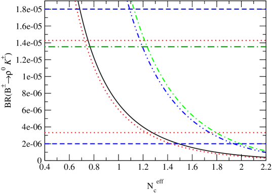
Figure 14: Branching ratio for $B^{\pm}\rightarrow\rho^{0}K^{\pm}$, for models $1(2)$, $k^{2}/m_{B}^{2}=0.3$ and limiting values of the CKM matrix elements. Solid line (dotted line) for model $(1)$ and max (min) CKM matrix elements. Dot-dashed line (dot-dot-dashed line) for model $(2)$ and max (min) CKM matrix elements. Notation: horizontal dotted line: CLEO data; dashed line: BABAR data; dot-dashed line: BELLE data.

In order to determine the range of $N_{c}^{eff}$ available for calculating the $CP$ violating parameter, $a$, in $B^{\pm,0}\rightarrow\rho^{0}K^{\pm,0}$, we have calculated the branching ratios for $B^{\pm}\rightarrow\rho^{0}K^{\pm}$, $B^{\pm}\rightarrow\rho^{\pm}K^{0}$, $B^{0}\rightarrow\rho^{\pm}K^{\mp}$, $B^{0}\rightarrow\rho^{0}K^{0}$, and $B^{\pm}\rightarrow\omega K^{\pm}$. We show all the results in Figs. 14, 15, 16, 17, and 18, where branching ratios are plotted as a function of $N_{c}^{eff}$ for models $(1)$ and $(2)$ (different form factors are used in models $(1)$ and $(2)$). By taking experimental data from CLEO, BABAR and BELLE Collaborations, listed in Table 7, and comparing theoretical predictions with experimental results, we expect to extract the allowed range of $N_{c}^{eff}$ in $B\rightarrow\rho K$ and to make the dependence on the form factors explicit between the two classes of models: models $(1,3)$ and $(5)$, and models $(2)$ and $(4)$. We shall mainly use the CLEO data, since the BABAR and BELLE data are (as yet) less numerous and accurate. An exception will be made for the branching ratio $B^{\pm}\rightarrow\omega K^{\pm}$, where we shall take the BELLE data for our analysis since they are the most accurate and most recent measurements in that case. Nevertheless, we shall also apply all of them to check the agreement between all the branching ratio data. The CLEO, BABAR and BELLE Collaborations give almost the same experimental branching ratios for all the investigated decays except for the decay $B^{-}\rightarrow\omega K^{-}$. In this later case, we observe a strong disagreement between all of them since they provide experimental data in a range from $0.1\times 10^{-6}$ to $12.8\times 10^{-6}$. Finally, it is evident that numerical results are very sensitive to uncertainties coming from the experimental data and from the factorization approach applied to calculate hadronic matrix elements in the $B\rightarrow K$ transition. Moreover, for $B\rightarrow\rho K$, the data are less numerous than for $B\rightarrow\rho\pi$, so we cannot expect to get a very accurate range of $N_{c}^{eff}$.

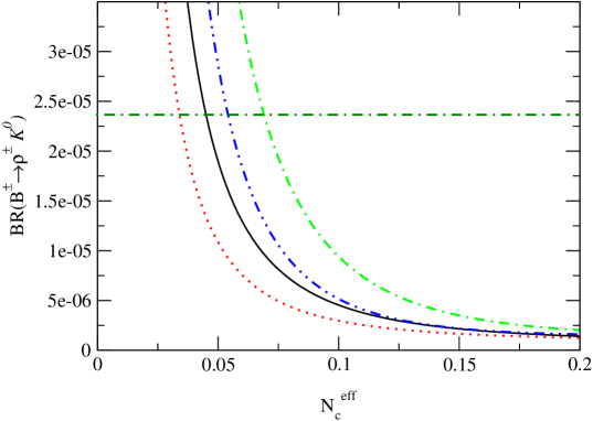
Figure 15: Branching ratio for $B^{\pm}\rightarrow\rho^{\pm}K^{0}$, for models $1(2)$, $k^{2}/m_{B}^{2}=0.3$ and limiting values of the CKM matrix elements. Solid line (dotted line) for model $(1)$ and max (min) CKM matrix elements. Dot-dashed line (dot-dot-dashed line) for model $(2)$ and max (min) CKM matrix elements. Same notation as in Fig. 14, but only experimental upper limits are available.

For the branching ratio $B^{\pm}\rightarrow\rho^{0}K^{\pm}$ (Fig. 14) we found a large range of values of $N_{c}^{eff}$ and CKM matrix elements over which the theoretical results are consistent with experimental data from CLEO, BABAR and BELLE. Each of the models, $(1,2,3,4)$ and $(5)$, gives an allowed range of $N_{c}^{eff}$. Even though strong differences appear between the two classes of models, because of the different used form factors, we are not able to draw strong conclusions about the dependence on the form factors. For the branching ratio $B^{\pm}\rightarrow\rho^{\pm}K^{0}$, (Fig. 15), BELLE gives only an upper branching ratio limit whereas BABAR and CLEO do not. Our predictions are still consistent with the experimental data for all models, for a large range of $N_{c}^{eff}$. In this case, the numerical results for models $(1)$ and $(2)$ are very close to each other and, we need new data to constrain our calculations.

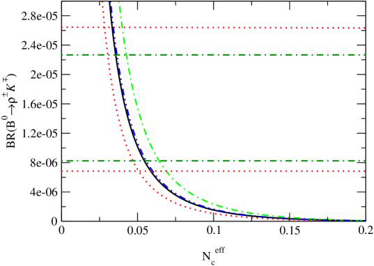
Figure 16: Branching ratio for $B^{0}\rightarrow\rho^{\pm}K^{\mp}$, for models $1(2)$, $k^{2}/m_{B}^{2}=0.3$ and limiting values of the CKM matrix elements. Solid line (dotted line) for model $(1)$ and max (min) CKM matrix elements. Dot-dashed line (dot-dot-dashed line) for model $(2)$ and max (min) CKM matrix elements. Same notation as in Fig. 14.

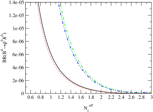
Figure 17: Branching ratio for $B^{0}\rightarrow\rho^{0}K^{0}$, for models $1(2)$, $k^{2}/m_{B}^{2}=0.3$ and limiting values of the CKM matrix elements. Solid line (dotted line) for model $(1)$ and max (min) CKM matrix elements. Dot-dashed line (dot-dot-dashed line) for model $(2)$ and max (min) CKM matrix elements.

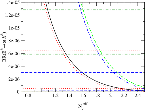
Figure 18: Branching ratio for $B^{\pm}\rightarrow\omega K^{\pm}$, for models $1(2)$, $k^{2}/m_{B}^{2}=0.3$ and limiting values of the CKM matrix elements. Solid line (dotted line) for model $(1)$ and max (min) CKM matrix elements. Dot-dashed line (dot-dot-dashed line) for model $(2)$ and max (min) CKM matrix elements. Same notation as in Fig. 14.

If we consider our results for the branching ratio $B^{0}\rightarrow\rho^{\pm}K^{\mp}$ (plotted in Fig. 16), there is agreement between the experimental results from CLEO and BELLE (no data from BABAR) and our theoretical predictions at very low values of $N_{c}^{eff}$ and the CKM matrix elements. All the models $(1,2,3,4)$ and $(5)$, give branching values within the range of branching ratio measurements if $N_{c}^{eff}$ is less than $0.07$. The tiny difference observed between models $(1)$ and $(2)$ comes from the form factor $A_{0}(k^{2})$ (where $A_{0}(k^{2})$ refers to the $B$ to $\rho$ transition taken at $k^{2}=m_{K}^{2}$) since in that case, the amplitude computed involves only the form factor $A_{0}(k^{2})$. For the branching ratio $B^{0}\rightarrow\rho^{0}K^{0}$ shown in Fig. 17, neither CLEO, BABAR nor BELLE give experimental results. Nevertheless, from models $(1)$ and $(2)$, it appears that this branching ratio is very sensitive to the magnitude of the form factor $F_{1}(k^{2})$ (in our case, $F_{1}(k^{2})$ is uncertain because $h_{1}=0.360$ or $0.762$ in models $(1)$ and $(2)$, respectively) since the tree contribution is only proportional to $F_{1}$. Moreover, from the range of allowed values of $N_{c}^{eff}$, we can estimate the upper limit of this branching ratio to be of the order $20\times 10^{-6}$. Finally, we focus on the branching ratio $B^{\pm}\rightarrow\omega K^{\pm}$ which is plotted in Fig. 18 for models $(1)$ and $(2)$. We find that both the experimental and theoretical results are in agreement for a large range of values of $N_{c}^{eff}$. But, the models $(1)$ and $(2)$ do not give similar results because the form factor $F_{1}$, applied in these models, is very different in both cases. Moreover, the dependence of the branching ratio on the CKM parameters $\rho$ and $\eta$ indicates that it would be possible to strongly constrain $\rho$ and $\eta$ with a very accurate experimental measurement for the decay $B^{-}\rightarrow\omega K^{-}$.

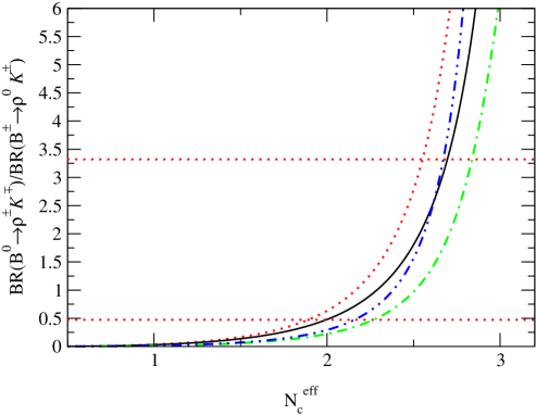
Figure 19: The ratio of two $\rho K$ branching ratios versus $N_{c}^{eff}$ for models $1(2)$ and for limiting values of the CKM matrix elements: solid line (dotted line) for model $(1)$ with max (min) CKM matrix elements. Dot-dashed line (dot-dot-dashed line) for model $(2)$ with max (min) CKM matrix elements. Same notation as in Fig. 14.

To remove systematic errors in branching ratios given by the $B$ factories, we look at the ratio, $R$, between the two following branching ratios: ${\rm BR}(B^{0}\rightarrow\rho^{\pm}K^{\mp})$ and ${\rm BR}(B^{\pm}\rightarrow\rho^{0}K^{\mp})$. The ratio is plotted in Fig. 19 as a function of $N_{c}^{eff}$, for models $(1)$ and $(2)$ and for limiting values of the CKM matrix elements. These results indicate that the ratio is very sensitive to both $N_{c}^{eff}$ and to the magnitude of the form factors. The sensitivity increases with the value of $N_{c}^{eff}$ and gives a large difference between models $(1,3)$ and $(5)$ and models $(2)$ and $(4)$. We found that for a definite range of $N_{c}^{eff}$, all models investigated give a ratio consistent with the experimental data from CLEO. It should be noted that $R$ is not very sensitive to the CKM matrix elements. Indeed, if we only take into account the tree contributions, $R$ is independent of the CKM parameters $\rho$ and $\eta$. The difference which appears comes from the penguin contribution and has to be taken into account in any approach since they are not negligible.

We have summarized for each model, each branching ratio and each set of limiting values of CKM matrix elements, the allowed range of $N_{c}^{eff}$ within which the experimental data and numerical results are consistent. To determine the best range of $N_{c}^{eff}$, we have to find some intersection of values of $N_{c}^{eff}$ for each model and each set of CKM matrix elements, for which the theoretical and experimental results are consistent. Since the experimental results are not numerous and not as accurate as one would like, it is more reasonable to fix the upper and lower limits of $N_{c}^{eff}$ which allow us the maximum of agreement between the theoretical and experimental approaches. By using the limiting values of the CKM matrix elements we show in Table 8, the range of allowed values of $N_{c}^{eff}$ with $\rho-\omega$ mixing. Even though in our previous study for $B\rightarrow\rho\pi$, we have restricted ourselves to models $(2)$ and $(4)$ rather than models $(1,3)$ and $(5)$, here, we cannot exclude one of the models $(1,2,3,4)$ and $(5)$ due to the lack of accurate experimental data. We find that $N_{c}^{eff}$ should be in the following range: $0.66(0.61)<N_{c}^{eff}<2.84(2.82)$, where the values outside and inside brackets correspond to the choice $k^{2}/m_{b}^{2}=0.3(0.5)$. Finally, if we take into account the allowed range of $N_{c}^{eff}$ determined for decays such as $B\rightarrow\rho\pi$ and $B\rightarrow\rho K$ we find a minimum global allowed range of $N_{c}^{eff}$ which should be in the range $1.17(1.12)<N_{c}^{eff}<1.63(1.77)$.

7 Summary and discussion

We have studied direct $CP$ violation in decay process such as $B^{\pm,0}\rightarrow\rho^{0}K^{\pm,0}\rightarrow\pi^{+}\pi^{-}K^{\pm,0}$ with the inclusion of $\rho-\omega$ mixing. When the invariant mass of the $\pi^{+}\pi^{-}$ pair is in the vicinity of the $\omega$ resonance, it is found that the $CP$ violating asymmetry, $a$, has a maximum $a_{max}$. We have also investigated the branching ratios $B^{0}\rightarrow\rho^{0}K^{0}$, $B^{0}\rightarrow\rho^{\pm}K^{\mp}$, $B^{\pm}\rightarrow\rho^{\pm}K^{0}$, $B^{\pm}\rightarrow\rho^{0}K^{\pm}$, and $B^{\pm}\rightarrow\omega K^{\pm}$. From our theoretical results, we make comparisons with experimental data from the CLEO, BABAR and BELLE Collaborations. We have applied five phenomenological models in order to show their dependence on form factors, CKM matrix elements and the effective parameter $N_{c}^{eff}$ in our approach.

To calculate the $CP$ violating asymmetry, $a$, and the branching ratios, we started from the weak Hamiltonian in which the OPE separates hard and soft physical regimes. We worked in the factorization approximation where the hadronic matrix elements are treated in some phenomenological quark models. The effective parameter, $N_{c}^{eff}$, was used in order to take into account, as well as possible, the non-factorizable effects involved in $B\rightarrow\rho K$ decays. Although one must have some doubts about factorization, it has been pointed out that it may be quite reliable in energetic weak decays [38].

With the present work, we have explicitly shown that the direct $CP$ violating asymmetry is very sensitive to the CKM matrix elements, the magnitude of the form factors $A_{0}(k^{2})$ and $F_{1}(k^{2})$, and also to the effective parameter $N_{c}^{eff}$ (in order of increasing dependence). We have determined a range for the maximum asymmetry, $a_{max}$, as a function of the parameter $N_{c}^{eff}$, the limits of CKM matrix elements and the choice of $k^{2}/m_{b}^{2}=0.3(0.5)$. For the decay ${\bar{B}}^{0}\rightarrow\pi^{+}\pi^{-}{\bar{K}}^{0}$ and from all models investigated, we found that the largest $CP$ violating asymmetry varies from $+37\%(+55\%)$ to $-20\%(-24\%)$. As regards $B^{-}\rightarrow\pi^{+}\pi^{-}K^{-}$, one gets $+49\%(+46\%)$ to $-22\%(-25\%)$. For $B^{\pm,0}\rightarrow\pi^{+}\pi^{-}K^{\pm,0}$, the sign of $a_{max}$ stays positive as long as the value of $N_{c}$ is less than $2.7$. In both decays, the ratio between asymmetry values which are taken at upper and lower limiting $\rho$ and $\eta$ values is mainly governed by the term $1/\sin\beta$. It appears also that the direct $CP$ violating asymmetry is very sensitive to the form factors at high values of $N_{c}^{eff}$. We underline that without the inclusion of $\rho-\omega$ mixing, we would not have a large $CP$ violating asymmetry, $a$, since $a$ is proportional to both $\sin\delta$ and $r$. We found a critical point for which $\sin\delta$ reaches the value $+1$, but at the same time, $r$ becomes very tiny. We emphazise that the advantage of $\rho-\omega$ mixing is the large strong phase difference which varies extremely rapidly near the $\omega$ resonance. In our calculations, we found that for $B^{\pm,0}\rightarrow\pi^{+}\pi^{-}K^{\pm,0}$, the sign of $\sin\delta$ is positive until $N_{c}^{eff}$ reaches $2.69(2.65)$ when $k^{2}/m_{b}^{2}=0.3(0.5)$. Then, by measuring $a$ for values of $N_{c}^{eff}$ lower than the limits given above, we can remove the phase uncertainty mod$(\pi)$ in the determination of the CKM angle $\gamma$.

As regards theoretical results for the branching ratios $B^{\pm}\rightarrow\rho^{0}K^{\pm}$, $B^{\pm}\rightarrow\rho^{\pm}K^{0}$, $B^{0}\rightarrow\rho^{\pm}K^{\mp}$, $B^{0}\rightarrow\rho^{0}K^{0}$ and $B^{\pm}\rightarrow\omega K^{\pm}$, we made comparison with data from the CLEO (mainly), BABAR and BELLE (for $B^{\pm}\rightarrow\omega K^{\pm}$) Collaborations. We found that it is possible to have agreement between the theoretical results and experimental branching ratio data for $B^{\pm}\rightarrow\rho^{0}K^{\pm}$, $B^{\pm}\rightarrow\rho^{\pm}K^{0}$, $B^{\pm}\rightarrow\omega K^{\pm}$, $B^{0}\rightarrow\rho^{\pm}K^{\mp}$, and $R$. For $B^{0}\rightarrow\rho^{0}K^{0}$, the lack of results does not allow us to draw conclusions. Only an estimation for the upper limit ($20\times 10^{-6}$) has been determined. Nevertheless, we have determined a range of value of $N_{c}^{eff}$, $0.66(0.61)<N_{c}^{eff}<2.84(2.82)$, inside of which the experimental data and theoretical calculations are consistent. We have to keep in mind that, because of the difficulty in dealing with non-factorizable effects associated with final state interactions (FSI), which are more complex for decays involving an $s$ quark, we have weakly constrained the range of value of $N_{c}^{eff}$.

¿From the $CP$ violating asymmetry and the branching ratios, we expect to determine the CKM matrix elements. In order to reach our aim, all uncertainties in our calculations have to be decreased: the transition form factors for $B\rightarrow\rho$ and $B\rightarrow K$ have to be well determined and non-factorizable effects have to be treated in the future by using generalized QCD factorization. Moreover, we strongly need more numerous and accurate experimental data in $B\rightarrow\rho K$ decays if we want to understand direct $CP$ violation in $B$ decays better.

Acknowledgments

This work was supported in part by the Australian Research Council and the University of Adelaide.

Figure captions

• Fig. 1 Tree diagram, for $B$ decays.

• Fig. 2 QCD-penguin diagram, for $B$ decays.

• Fig. 3 Electroweak-penguin diagram, for $B$ decays.

• Fig. 4 Electroweak-penguin diagram (coupling between $Z,\gamma$ and $W$), for $B$ decays.

• Fig. 5 $B$ decays without (upper) and with (lower) $\rho-\omega$ mixing.

• Fig. 6 $CP$ violating asymmetry, $a$, for ${\bar{B}}^{0}\rightarrow\pi^{+}\pi^{-}{\bar{K}}^{0}$, for $k^{2}/m_{b}^{2}=0.3$, for $N_{c}^{eff}=0.66,2.69,2.84$ and for limiting values, max (min), of the CKM matrix elements for model $(1)$: dot-dot-dashed line (dot-dash-dashed line) for $N_{c}^{eff}=0.66$. Solid line (dotted line) for $N_{c}^{eff}=2.69$. Dashed line (dot-dashed line) for $N_{c}^{eff}=2.84$.

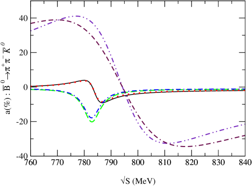
Figure 7: $CP$ violating asymmetry, $a$, for ${\bar{B}}^{0}\rightarrow\pi^{+}\pi^{-}{\bar{K}}^{0}$, for $k^{2}/m_{b}^{2}=0.5$, for $N_{c}^{eff}=0.61,2.65,2.82$ and for limiting values, max (min), of the CKM matrix elements for model $(1)$: dot-dot-dashed line (dot-dash-dashed line) for $N_{c}^{eff}=0.61$. Solid line (dotted line) for $N_{c}^{eff}=2.65$. Dashed line (dot-dashed line) for $N_{c}^{eff}=2.82$.

• Fig. 7 $CP$ violating asymmetry, $a$, for ${\bar{B}}^{0}\rightarrow\pi^{+}\pi^{-}{\bar{K}}^{0}$, for $k^{2}/m_{b}^{2}=0.5$, for $N_{c}^{eff}=0.61,2.65,2.82$ and for limiting values, max (min), of the CKM matrix elements for model $(1)$: dot-dot-dashed line (dot-dash-dashed line) for $N_{c}^{eff}=0.61$. Solid line (dotted line) for $N_{c}^{eff}=2.65$. Dashed line (dot-dashed line) for $N_{c}^{eff}=2.82$.

• Fig. 8 $CP$ violating asymmetry, $a$, for $B^{-}\rightarrow\pi^{+}\pi^{-}K^{-}$, for $k^{2}/m_{b}^{2}=0.3$, for $N_{c}^{eff}=0.66,2.69,2.84$ and for limiting values, max (min), of the CKM matrix elements for model $(1)$: dot-dot-dashed line (dot-dash-dashed line) for $N_{c}^{eff}=0.66$. Solid line (dotted line) for $N_{c}^{eff}=2.69$. Dashed line (dot-dashed line) for $N_{c}^{eff}=2.84$.

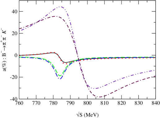
Figure 9: $CP$ violating asymmetry, $a$, for $B^{-}\rightarrow\pi^{+}\pi^{-}K^{-}$, for $k^{2}/m_{b}^{2}=0.5$, for $N_{c}^{eff}=0.61,2.65,2.82$ and for limiting values, max (min), of the CKM matrix elements for model $(1)$: dot-dot-dashed line (dot-dash-dashed line) for $N_{c}^{eff}=0.61$. Solid line (dotted line) for $N_{c}^{eff}=2.65$. Dashed line (dot-dashed line) for $N_{c}^{eff}=2.82$.

• Fig. 9 $CP$ violating asymmetry, $a$, for $B^{-}\rightarrow\pi^{+}\pi^{-}K^{-}$, for $k^{2}/m_{b}^{2}=0.5$, for $N_{c}^{eff}=0.61,2.65,2.82$ and for limiting values, max (min), of the CKM matrix elements for model $(1)$: dot-dot-dashed line (dot-dash-dashed line) for $N_{c}^{eff}=0.61$. Solid line (dotted line) for $N_{c}^{eff}=2.65$. Dashed line (dot-dashed line) for $N_{c}^{eff}=2.82$.

• Fig. 10 $\sin\delta$, as a function of $N_{c}^{eff}$, for ${\bar{B}}^{0}\rightarrow\pi^{+}\pi^{-}{\bar{K}}^{0}$, for $k^{2}/m_{B}^{2}=0.3(0.5)$ and for model $(1)$. The solid (dotted) line at $\sin\delta=+1$ corresponds the case $\tilde{\Pi}_{\rho\omega}=(-3500;-300)$, where $\rho-\omega$ mixing is included. The dot-dashed (dot-dot-dashed) line corresponds to $\tilde{\Pi}_{\rho\omega}=(0;0)$, where $\rho-\omega$ mixing is not included.

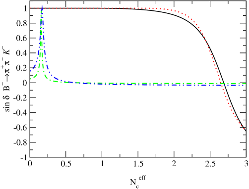
Figure 11: $\sin\delta$, as a function of $N_{c}^{eff}$ for $B^{-}\rightarrow\pi^{+}\pi^{-}K^{-}$, for $k^{2}/m_{B}^{2}=0.3(0.5)$ and for model $(1)$. The solid (dotted) line at $\sin\delta=+1$ corresponds to the case $\tilde{\Pi}_{\rho\omega}=(-3500;-300)$, where $\rho-\omega$ mixing is included. The dot-dashed (dot-dot-dashed) line corresponds to $\tilde{\Pi}_{\rho\omega}=(0;0)$, where $\rho-\omega$ mixing is not included.

• Fig. 11 $\sin\delta$, as a function of $N_{c}^{eff}$, for $B^{-}\rightarrow\pi^{+}\pi^{-}K^{-}$, for $k^{2}/m_{B}^{2}=0.3(0.5)$ and for model $(1)$. The solid (dotted) line at $\sin\delta=+1$ corresponds the case $\tilde{\Pi}_{\rho\omega}=(-3500;-300)$, where $\rho-\omega$ mixing is included. The dot-dashed (dot-dot-dashed) line corresponds to $\tilde{\Pi}_{\rho\omega}=(0;0)$, where $\rho-\omega$ mixing is not included.

• Fig. 12 The ratio of penguin to tree amplitudes, $r$, as a function of $N_{c}^{eff}$, for ${\bar{B}}^{0}\rightarrow\pi^{+}\pi^{-}{\bar{K}}^{0}$, for $k^{2}/m_{B}^{2}=0.3(0.5)$, for limiting values of the CKM matrix elements $(\rho,\eta)$ max(min), for $\tilde{\Pi}_{\rho\omega}=(-3500;-300)(0,0)$, (i.e. with(without) $\rho-\omega$ mixing) and for model $(1)$. Figure 12a (left): for $\tilde{\Pi}_{\rho\omega}=(0;0)$, solid line (dotted line) for $k^{2}/m_{B}^{2}=0.3$ and $(\rho,\eta)$ max(min). Dot-dashed line (dot-dot-dashed line) for $k^{2}/m_{B}^{2}=0.5$ and $(\rho,\eta)$ max(min). Figure 12b (right): same caption but for $\tilde{\Pi}_{\rho\omega}=(-3500;-300)$.

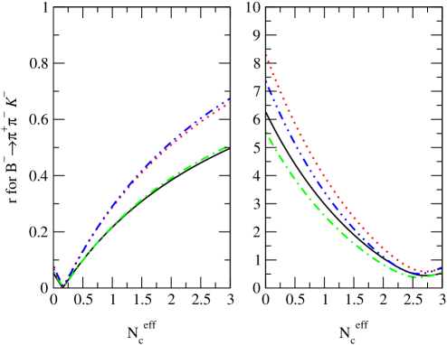
Figure 13: The ratio of penguin to tree amplitudes, $r$, for $B^{-}\rightarrow\pi^{+}\pi^{-}K^{-}$. Same caption for Figure 13a (left) and Figure 13b (right) as in Fig. 12.

• Fig. 13 The ratio of penguin to tree amplitudes, $r$, for $B^{-}\rightarrow\pi^{+}\pi^{-}K^{-}$. Same caption for Figure 13a (left) and Figure 13b (right) as in Fig. 12.

• Fig. 14 Branching ratio for $B^{\pm}\rightarrow\rho^{0}K^{\pm}$, for models $1(2)$, $k^{2}/m_{B}^{2}=0.3$ and limiting values of the CKM matrix elements. Solid line (dotted line) for model $(1)$ and max (min) CKM matrix elements. Dot-dashed line (dot-dot-dashed line) for model $(2)$ and max (min) CKM matrix elements.

• Fig. 15 Branching ratio for $B^{\pm}\rightarrow\rho^{\pm}K^{0}$, for models $1(2)$, $k^{2}/m_{B}^{2}=0.3$ and limiting values of the CKM matrix elements. Solid line (dotted line) for model $(1)$ and max (min) CKM matrix elements. Dot-dashed line (dot-dot-dashed line) for model $(2)$ and max (min) CKM matrix elements.

• Fig. 16 Branching ratio for $B^{0}\rightarrow\rho^{\pm}K^{\mp}$, for models $1(2)$, $k^{2}/m_{B}^{2}=0.3$ and limiting values of the CKM matrix elements. Solid line (dotted line) for model $(1)$ and max (min) CKM matrix elements. Dot-dashed line (dot-dot-dashed line) for model $(2)$ and max (min) CKM matrix elements.

• Fig. 17 Branching ratio for $B^{0}\rightarrow\rho^{0}K^{0}$, for models $1(2)$, $k^{2}/m_{B}^{2}=0.3$ and limiting values of the CKM matrix elements. Solid line (dotted line) for model $(1)$ and max (min) CKM matrix elements. Dot-dashed line (dot-dot-dashed line) for model $(2)$ and max (min) CKM matrix elements.

• Fig. 18 Branching ratio for $B^{\pm}\rightarrow\omega K^{\pm}$, for models $1(2)$, $k^{2}/m_{B}^{2}=0.3$ and limiting values of the CKM matrix elements. Solid line (dotted line) for model $(1)$ and max (min) CKM matrix elements. Dot-dashed line (dot-dot-dashed line) for model $(2)$ and max (min) CKM matrix elements.

• Fig. 19 The ratio of the two $\rho K$ branching ratios versus $N_{c}^{eff}$ for models $1(2)$ and for limiting values of the CKM matrix elements: solid line (dotted line) for model $(1)$ with max (min) CKM matrix elements. Dot-dashed line (dot-dot-dashed line) for model $(2)$ with max (min) CKM matrix elements.

Table captions

• Table 1 Wilson coefficients to the next-leading order.

• Table 2 Effective Wilson coefficients related to the tree operators, electroweak and QCD-penguin operators.

• Table 3 Values of the CKM unitarity triangle for limiting values of the CKM matrix elements.

• Table 4 Form factor values for $B\rightarrow\rho$ and $B\rightarrow K$ at $q^{2}=0$.

• Table 5 Maximum $CP$ violating asymmetry $a_{max}(\%)$ for ${\bar{B}}^{0}\rightarrow\pi^{+}\pi^{-}{\bar{K}}^{0}$, for all models, limiting values of the CKM matrix elements (upper and lower limit), and for $k^{2}/m_{b}^{2}=0.3(0.5)$.

• Table 6 Maximum $CP$ violating asymmetry $a_{max}(\%)$ for $B^{-}\rightarrow\pi^{+}\pi^{-}K^{-}$, for all models, limiting values of the CKM matrix elements (upper and lower limit), and for $k^{2}/m_{b}^{2}=0.3(0.5)$.

• Table 7 The measured branching ratios by CLEO, BABAR and BELLE factories for $B$ decays into $\rho K$ ($10^{-6}$).

• Table 8 Best range of $N_{c}^{eff}$ determined for $k^{2}/m_{b}^{2}=0.3(0.5)$ and for $B\rightarrow\rho K$ decays (upper). Also range of $N_{c}^{eff}$ determined previously for $B\rightarrow\rho\pi$ decays [39] (updated). Finally global range of $N_{c}^{eff}$ from both $B$ decays (lower).

$C_{i}(\mu)$ for $\mu=5$ GeV
	$C_{1}$	$-0.3125$
	$C_{2}$	$+1.1502$
$C_{3}$	$+0.0174$	$C_{5}$	$+0.0104$
$C_{4}$	$+0.0373$	$C_{6}$	$-0.0459$
$C_{7}$	$-1.050\times 10^{-5}$	$C_{9}$	$-0.0101$
$C_{8}$	$+3.839\times 10^{-4}$	$C_{10}$	$+1.959\times 10^{-3}$

Table 1: Wilson coefficients to the next-leading order (see the reference in text).

$C_{i}^{\prime}$	$q^{2}/m_{b}^{2}=0.3$	$q^{2}/m_{b}^{2}=0.5$
$C_{1}^{\prime}$	$-0.3125$	$-0.3125$
$C_{2}^{\prime}$	$+1.1502$	$+1.1502$
$C_{3}^{\prime}$	$+2.433\times 10^{-2}+1.543\times 10^{-3}i$	$+2.120\times 10^{-2}+2.174\times 10^{-3}i$
$C_{4}^{\prime}$	$-5.808\times 10^{-2}-4.628\times 10^{-3}i$	$-4.869\times 10^{-2}-1.552\times 10^{-2}i$
$C_{5}^{\prime}$	$+1.733\times 10^{-2}+1.543\times 10^{-3}i$	$+1.420\times 10^{-2}+5.174\times 10^{-3}i$
$C_{6}^{\prime}$	$-6.668\times 10^{-2}-4.628\times 10^{-3}i$	$-5.729\times 10^{-2}-1.552\times 10^{-2}i$
$C_{7}^{\prime}$	$-1.435\times 10^{-4}-2.963\times 10^{-5}i$	$-8.340\times 10^{-5}-9.938\times 10^{-5}i$
$C_{8}^{\prime}$	$+3.839\times 10^{-4}$	$+3.839\times 10^{-4}$
$C_{9}^{\prime}$	$-1.023\times 10^{-2}-2.963\times 10^{-5}i$	$-1.017\times 10^{-2}-9.938\times 10^{-5}i$
$C_{10}^{\prime}$	$+1.959\times 10^{-3}$	$+1.959\times 10^{-3}$

Table 2: Effective Wilson coefficients related to the tree operators, electroweak and QCD penguin operators (see the reference in text).

	$\alpha$	$\beta$	$\gamma$
$(\rho_{min},\eta_{min})$	$104^{o}47$	$19^{o}32$	$56^{o}21$
$(\rho_{min},\eta_{max})$	$93^{o}13$	$24^{o}31$	$62^{o}56$
$(\rho_{max},\eta_{min})$	$112^{o}14$	$21^{o}20$	$46^{o}66$
$(\rho_{max},\eta_{max})$	$99^{o}66$	$26^{o}56$	$53^{o}78$

Table 3: Values of the CKM unitarity triangle for limiting values of the CKM matrix elements.

	$h_{A_{0}}$	$h_{1}$	$m_{A_{0}}$	$m_{1}$	$d_{0}(d_{1})$	$b_{0}(b_{1})$
model $(1)$	0.280	0.360	5.27	5.41
model $(2)$	0.340	0.762	5.27	5.41
model $(3)$	0.280	0.360	5.27	5.41
model $(4)$	0.340	0.762	5.27	5.41
model $(5)$	0.372	0.341			1.400(0.410)	0.437(-0.361)

Table 4: Form factor values for $B\rightarrow\rho$ and $B\rightarrow K$ at $q^{2}=0$ (see the reference in text).

	$N_{cmin}^{eff}=0.66(0.61)$	$N_{cmax}^{eff}=2.84(2.82)$
model $(1)$
$\rho_{max},\eta_{max}$	32(46)	-14(-16)
$\rho_{min},\eta_{min}$	25(33)	-19(-22)
model $(2)$
$\rho_{max},\eta_{max}$	32(41)	-6(-7)
$\rho_{min},\eta_{min}$	27(30)	-9(-10)
model $(3)$
$\rho_{max},\eta_{max}$	32(45)	-14(-16)
$\rho_{min},\eta_{min}$	25(33)	-20(-23)
model $(4)$
$\rho_{max},\eta_{max}$	32(41)	-6(-7)
$\rho_{min},\eta_{min}$	27(30)	-9(-10)
model $(5)$
$\rho_{max},\eta_{max}$	37(55)	-15(-17)
$\rho_{min},\eta_{min}$	26(40)	-19(-24)

Table 5: Maximum $CP$ violating asymmetry $a_{max}(\%)$ for ${\bar{B}}^{0}\rightarrow\pi^{+}\pi^{-}{\bar{K}}^{0}$, for all models, limiting values (upper and lower) of the CKM matrix elements, and for $k^{2}/m_{b}^{2}=0.3(0.5)$.

	$N_{cmin}^{eff}=0.66(0.61)$	$N_{cmax}^{eff}=2.84(2.82)$
model $(1)$
$\rho_{max},\eta_{max}$	47(45)	-15(-17)
$\rho_{min},\eta_{min}$	34(35)	-21(-23)
model $(2)$
$\rho_{max},\eta_{max}$	45(41)	-11(-13)
$\rho_{min},\eta_{min}$	33(32)	-17(-18)
model $(3)$
$\rho_{max},\eta_{max}$	47(44)	-15(-17)
$\rho_{min},\eta_{min}$	34(35)	-20(-23)
model $(4)$
$\rho_{max},\eta_{max}$	45(42)	-12(-13)
$\rho_{min},\eta_{min}$	33(32)	-17(-18)
model $(5)$
$\rho_{max},\eta_{max}$	49(46)	-17(-19)
$\rho_{min},\eta_{min}$	36(35)	-22(-25)

Table 6: Maximum $CP$ violating asymmetry $a_{max}(\%)$ for $B^{-}\rightarrow\pi^{+}\pi^{-}K^{-}$, for all models, limiting values of the CKM matrix elements (upper and lower limit), and for $k^{2}/m_{b}^{2}=0.3(0.5)$.

	CLEO	BABAR	BELLE
$\rho^{0}K^{\pm}$	${8.46^{+4.0}_{-3.4}\pm 1.8}^{\bullet}$ ${(\leq 17)}^{\P}$	${10\pm 6\pm 2}^{\star}$ ${(\leq 29)}^{\P}$	${\leq 13.5}^{\P}$
$\rho^{\pm}K^{0}$	$-$	$-$	${\leq 23.6}^{\P}$
$\rho^{\pm}K^{\mp}$	${16.0^{+7.6}_{-6.4}\pm 2.8}^{\bullet}$ ${(\leq 32)}^{\P}$	$-$	${15.8^{+5.1\;+1.7}_{-4.6\;-3.0}}^{\star}$
$\rho^{0}K^{0}$	$-$	$-$	$-$
$\frac{BR(\rho^{\pm}K^{\mp})}{BR(\rho^{0}K^{\pm})}$	$1.89\pm 1.41$	$-$	$-$
$\omega K^{\pm}$	${3.2^{+2.4}_{-1.9}\pm 0.8}^{\bullet}$ ${(\leq 7.9)}^{\P}$	${1.4^{+1.3}_{-1.0}\pm 0.3}^{\star}$	${9.2^{+2.6}_{-2.3}\pm 1.0}^{\star}$

Table 7: The measured branching ratios by CLEO, BABAR and BELLE factories for $B$ decays into $\rho K$ ($10^{-6}$) (see the reference in text). ${\rm Experimental\;data}^{\star}$, ${\rm fit}^{\bullet}$ and ${\rm upper\;limit}^{\P}$.

$B\rightarrow\rho K$	$\left\{N_{c}^{eff}\right\}$
model $(1)$	0.66;2.68(0.61;2.68)
model $(2)$	1.17;2.84(1.09;2.82)
maximum range	0.66;2.84(0.61;2.82)
minimum range	1.17;2.68(1.09;2.68)
$B\rightarrow\rho\pi$	$\left\{N_{c}^{eff}\right\}$
model $(2)$	1.09;1.63(1.12;1.77)
model $(4)$	1.10;1.68(1.11;1.80)
maximum range	1.09;1.68(1.11;1.80)
minimum range	1.10;1.63(1.12;1.77)
global range	$\left\{N_{c}^{eff}\right\}$
global maximum range	0.66;2.84(0.61;2.82)
global minimum range	1.17;1.63(1.12;1.77)

Table 8: Best range of $N_{c}^{eff}$ determined for $k^{2}/m_{b}^{2}=0.3(0.5)$ and for $B\rightarrow\rho K$ decays (upper). Also range of $N_{c}^{eff}$ determined previously for $B\rightarrow\rho\pi$ decays [39] (updated). Finally global range of $N_{c}^{eff}$ from both $B$ decays (lower).

References

- [1] A.B. Carter and A.I. Sanda, Phys. Rev. Lett. 45 (1980) 952, Phys. Rev. D23 (1981) 1567; I.I. Bigi and A.I. Sanda, Nucl. Phys. B193 (1981) 85.
- [2] Proceedings of the Workshop on Violation, Adelaide 1998, edited by X.-H. Guo, M. Sevior and A.W. Thomas (World Scientific, Singapore).
- [3] R. Enomoto and M. Tanabashi, Phys. Lett. B386 (1996) 413.
- [4] S. Gardner, H.B. O’Connell and A.W. Thomas, Phys. Rev. Lett. 80 (1998) 1834.
- [5] X.-H. Guo and A.W. Thomas, Phys. Rev. D58 (1998) 096013, Phys. Rev. D61 (2000) 116009.
- [6] A.J. Buras, Lect. Notes Phys. 558 (2000) 65, also in ‘Recent Developments in Quantum Field Theory’, Springer Verlag, edited by P. Breitenlohner, D. Maison and J. Wess (Springer-Verleg, Berlin, in press), hep-ph/9901409.
- [7] V.A. Novikov, M.A. Shifman, A.I. Vainshtein and V.I. Zakharov, Nucl. Phys. B249 (1985) 445, Yad. Fiz. 41 (1985) 1063.
- [8] M.A. Shifman, A.I. Vainshtein and V.I. Zakharov, Nucl. Phys. B147 (1979) 385, Nucl. Phys. B147 (1979) 448.
- [9] A.J. Buras, Published in ‘Probing the Standard Model of Particle Interactions’, eds. 1998, Elsevier Science B.V., hep-ph/9806471.
- [10] N.G. Deshpande and X.-G. He, Phys. Rev. Lett. 74 (1995) 26.
- [11] R. Fleischer, Int. J. Mod. Phys. A12 (1997) 2459, Z. Phys. C62 (1994) 81, Z. Phys. C58 (1993) 483.
- [12] G. Kramer, W. Palmer and H. Simma, Nucl. Phys. B428 (1994) 77.
- [13] G. Buchalla, A.J. Buras and M.E. Lautenbacher, Rev. Mod. Phys. 68, (1996) 1125.
- [14] M. Beneke, Published in Budapest 2001, High Energy Physics, hep-ph/0201137.
- [15] L. Wolfenstein, Phys. Rev. Lett. 51 (1983) 1945, Phys. Rev. Lett. 13 (1964) 562.
- [16] J.J. Sakurai, Currents and Mesons, University of Chicago Press (1969).
- [17] H.B. O’Connell, B.C. Pearce, A.W. Thomas and A.G. Williams, Prog. Part. Nucl. Phys. 39 (1997) 201; H.B. O’Connell, A.G. Williams, M. Bracco and G. Krein, Phys. Lett. B370 (1996) 12; H.B. O’Connell, Aust. J. Phys. 50 (1997) 255.
- [18] The Particle Data Group, D.E. Groom et al., Eur. Phys. J. C15 (2000) 1.
- [19] H.B. O’Connell, A.W. Thomas and A.G. Williams, Nucl. Phys. A623 (1997) 559; K. Maltman, H.B. O’Connell and A.G. Williams, Phys. Lett. B376 (1996) 19.
- [20] S. Gardner and H.B. O’Connell, Phys. Rev. D57 (1998) 2716.
- [21] J. Schwinger, Phys. Rev. 12 (1964) 630; D. Farikov and B. Stech, Nucl. Phys. B133 (1978) 315; N. Cabibbo and L. Maiani, Phys. Lett. B73 (1978) 418; M.J. Dugan and B. Grinstein, Phys. Lett. B255 (1991) 583.
- [22] M. Bauer, B. Stech and M. Wirbel, Z. Phys. C34 (1987) 103; M. Wirbel, B. Stech and M. Bauer, Z. Phys. C29 (1985) 637.
- [23] J.D. Bjorken, Nucl. Phys. Proc. Suppl. 11 (1989) 325.
- [24] X.-H. Guo and T. Huang, Phys. Rev. D43 (1991) 2931.
- [25] P. Ball, JHEP 9809 (1998) 005.
- [26] P. Ball and V.M. Braun, Phys. Rev. D58 (1998) 094016.
- [27] Y.-H. Chen, H.-Y. Cheng, B. Tseng and K.-C. Yang, Phys. Rev. D60 (1999) 094014.
- [28] By ALEPH Collaboration, CDF Collaboration, DELPHI Collaboration, L3 Collaboration, OPAL Collaboration and SLD Collaboration (D. Abbaneo et al.), hep-ex/0112028.
- [29] H.-Y. Cheng and A. Soni, Phys. Rev. D64 (2001) 114013.
- [30] D. Melikhov and B. Stech, Phys. Rev. D62 (2000) 014006.
- [31] H.-Y. Cheng and B. Tseng, hep-ph/9708211.
- [32] C.P. Jessop, et al. (CLEO Collaboration), Phys. Rev. Lett. 85 (2000) 2881.
- [33] A. Bozek (BELLE Collaboration), in Proceedings of the 4th International Conference on B Physics and Violation, Ise-Shima, Japan, February 2001, hep-ex/0104041.
- [34] K. Abe, et al. (BELLE Collaboration), in Proceedings of the XX International Symposium on Lepton and Photon Interactions at High Energies, July 2001, Roma, Italy, BELLE-CONF-0115 (2001).
- [35] K. Abe, et al. (BELLE Collaboration), Phys. Rev. D65 (2002) 092005; R.S. Lu, et al. (BELLE Collaboration), hep-ex/0207019 (Submitted to Phys. Rev. Lett.).
- [36] T. Schietinger (BABAR Collaboration), Proceedings of the Lake Louise Winter Institute on Fundamental Interactions, Alberta, Canada, February 2001, hep-ex/0105019.
- [37] B. Aubert, et al. (BABAR Collaboration), hep-ex/0008058; B. Aubert, et al. (BABAR Collaboration), Phys. Rev. Lett. 87 (2001) 221802.
- [38] H.-Y. Cheng, Phys. Lett. B335 (1994) 428, Phys. Lett. B395 (1997) 345; H.-Y. Cheng and B. Tseng, Phys. Rev. D58 (1998) 094005.
- [39] X.-H. Guo, O. Leitner and A.W. Thomas, Phys. Rev. D63 (2001) 056012.