Abstract

We explore the usefulness of the existing relations between the $S$-matrix and time delay in characterizing baryon resonances in pion-nucleon scattering. We draw attention to the fact that the existence of a positive maximum in time delay is a necessary criterion for the existence of a resonance and should be used as a constraint in conventional analyses which locate resonances from poles of the $S$-matrix and Argand diagrams. The usefulness of the time delay plots of resonances is demonstrated through a detailed analysis of the time delay in several partial waves of $\pi N$ elastic scattering.

PACS numbers: 14.20.Gk, 13.85.Dz, 03.65.Nk

1 Introduction

Ever since the discovery of the first excited nucleon state [1], the baryon resonances have played a major role in particle and nuclear physics and have contributed crucially to the search of the fundamental building blocks of nature. We perceive them now as the low energy manifestation of quantum chromodynamics (QCD) with three quark degrees of freedom. However, low energy QCD is still not well understood and very often one is left with models. The status of the resonances can differ from case to case as can their parameters extracted from different experiments. The $N^{*}$ programs at Jefferson Lab [2] and the forthcoming Japan Hadron Facility [3] have both revived the area. The various theoretical studies [4-7] and the hope to find exotic hadrons [8], make the area once again an exciting field of physics. It is then justified to look at the baryon resonances from a yet different perspective and to analyze the existing data in a novel albeit well established way, while waiting for new experimental results. Specifically, we refer to the time delay method which was introduced into scattering theory and especially resonance physics by Eisenbud and Wigner [9, 10, 11]. In view of the considerable number of standard textbooks [12-17] and numerous papers [9-11,18-39] published since the seminal paper by Wigner [10], we provide only a short introduction. Time delay is a measure of the collision time in a scattering reaction which can be calculated directly from the phase shift or the $T$ matrix. Obviously, such a concept has a close connection to the appearance of an unstable intermediate state (resonance), which, due to its finite lifetime, “delays” the reaction. Though the interest in time delay ever since the first papers was unabated, it is only recently that it has been used in practice in quantum scattering theory (in chaotic scattering [40], hadron resonances [33,37-39] and heavy ion collisions [35]) and tunneling phenomena [36], with success. The present work is simply a logical extension of this program carried over to baryon resonances, partly done already in [37].

To identify the baryon resonances, one performs a partial wave analysis of the meson baryon scattering data and obtains the energy dependent amplitude (or $T$-matrix) by fitting cross section data. Resonances are then determined by locating the poles of the $T$-matrix on the unphysical sheet and studying the Argand diagrams of the complex $T$-matrix. Due to model dependence in the analyses of the energy-dependent amplitudes, there are differences in the resonance parameters quoted by different groups [41]. The resonance receiving confirmation from several analyses is considered to be well established. Though we do not dispute the usefulness of the pole of the $S$-matrix, we note that there exist several views in literature, regarding the definition of a resonance. In a review article [42], Dalitz discussed various criteria for the existence of a resonance elaborately, with the conclusion that for the case of a pole in the $S$-matrix, $S(E)$, in the unphysical E-plane lying sufficiently close to the physical E axis, there is no ambiguity in the conclusion of the existence of a resonance. However, the authors in [43] constructed examples in such a way that a sharp resonance was produced without an accompanying pole in the unphysical sheet. They noted that even the inverse correspondence, namely, (pole of the $S$-matrix on the unphysical sheet) $\rightarrow$ (unstable particle) may be questioned. In [44], it was pointed out that a peak in the cross section cannot be conclusive evidence of a resonance. In [45], in addition to time delay, the exponential decay law was required as a signal of a genuine resonance (this may be in view of the existence of double poles, which would lead to a non-exponential decay [46]). Cautious remarks on the use of Argand diagrams can be found in [19, 47]. The many different opinions reflect only the fact that the issue is not yet satisfactorily settled. Indeed, unstable particles remained to be problematic even until now [48]. We make use of the requirement stated in literature and text books [9-39], namely, the formation of a resonance should introduce a large positive time delay in the scattering of particles. We try to extract resonance parameters from the energy distribution of time delay by locating the position of the local maximum and reading off the width as advocated e.g. in [49]. Though the non-resonant background can deform the positive resonant structure in the vicinity of a resonance, we do expect some positive region around the resonance point, with perhaps a less dominant peak. This is confirmed by our study.

Starting with the definition of time delay in terms of the $S$-matrix, we obtain its relation with the $T$-matrix and scattering phase shifts. We shall first demonstrate the usefulness of the method with examples of well-known $N$ and $\Delta$ resonances. Later on we proceed to the analysis of time delay in various partial waves of $\pi N$ elastic scattering, using the available single energy values as well as some energy-dependent forms of the $T$-matrix. Before we move on to the discussion of time delay, it is important to note that the time delay plots of the present work are not the same as speed plots [50] which have been sometimes referred to as time delay plots in literature. Speed plots are positive definite by definition. Time delay plots can also assume negative values and only a positive peak signals a resonance. In the elastic region, the speed is equal to time delay up to a constant factor, but once the inelastic channels open up, this is no longer true [37].

Considering the fact that the time delay method has so far not been applied to baryon resonances (but has been successfully applied to meson resonances [39]), our study is a practical test of time delay when applied directly to data. When applied to theoretical $T$ matrix solutions, we could say that indeed the model is being tested, if we consider the resonances to be well established.

In passing, we note that time delay is also related to the so called arrival time in quantum mechanics [51] and has also been used to obtain the density of resonances [52].

2 Time delay in resonant scattering

We shall now discuss the expressions which quantify time delay and can hence be used to characterize resonances.

2.1 Relation to phase shifts

In the early fifties, using a wave packet analysis, Bohm [15], Eisenbud [9] and Wigner [10], obtained an expression for the time delay $\Delta t$ in binary collisions. In the case of elastic scattering, they derived $\Delta t$ in terms of the energy derivative of the scattering phase shift as follows:

$$\Delta t=2\hbar{d\delta\over dE}\,.$$ (1)

The formation of a resonance in a scattering process, introduces a positive time delay between the arrival of the incident wave packet and its departure from the collision region. From the above relation, one expects the phase shift to increase rapidly in the vicinity of a resonance.

The wave packet analysis of time delay was extended by Eisenbud to inelastic collisions [9]. He defined the delay time matrix $\Delta t$, such that an element $\Delta t_{ij}$ of this matrix, corresponded to the time interval between the outgoing wave in channel $j$ and the ingoing wave in channel $i$. This time delay, $\Delta t_{ij}$, is related to the $S$-matrix as follows:

$$\Delta t_{ij}=Re\big{[}-i\hbar(S_{ij})^{-1}{dS_{ij}\over dE}\big{]}\,.$$ (2)

Before we proceed further, we note that the phase shifts, in principle, depend on the orbital angular momenta, $l$, $l^{\prime}$, of the initial and final states respectively and on the total angular momentum $J$. However, we have suppressed this dependence in the expressions whenever not relevant. In the present work, we consider $\pi N$ elastic scattering, which is the scattering of a spin zero and spin one half particle. Since the total spin in the final and initial state is $S=S^{\prime}=1/2$ and conservation of parity gives $l=l^{\prime}$, the total angular momentum $J$ takes the values $l-1/2$ and $l+1/2$. The $S$-matrix is diagonal in $l$ and its elements are related to phase shifts as $S_{ll}^{J}=exp(2i\delta^{J})$, for the elastic case in the absence of inelasticities.

We see that in the case of purely elastic scattering ($j=i$), and using a phase shift formulation for the $S$-matrix where $S=e^{2i\delta}$, we get,

$$\Delta t_{ii}=2\hbar{d\delta\over dE}\,,$$ (3)

which is the same as Eq. (1). These $\Delta t_{ii}$ are related to the lifetimes of metastable states or resonances in elastic scattering (see [18]). At high energies, where apart from elastic scattering, the possibility of scattering into inelastic channels also opens up, the elastic $S$-matrix element is defined as $S=\eta e^{2i\delta}$, where $\eta$ is the inelasticity parameter defined such that $0<\eta\leq 1$. Substituting the modified $S$ (i.e. $S=\eta e^{2i\delta}$) in Eq. (2), gives,

$$\Delta t_{ii} = Re\biggl{[}\,-i\hbar\,\biggl{(}\,2i{d\delta\over dE}+{d\eta\over dE}\,{1\over\eta}\,\biggr{)}\biggr{]}\,\,=\,2\hbar\,{d\delta\over dE}\,.$$ (4)

The above equation is the same as Eqs (1) and (3). Thus it can be seen that the expression for the time delay, $\Delta t_{ii}$, for elastic scattering is the same, irrespective of the presence of inelastic channels.

It is clear from the above expressions that time delay can also take negative values resulting from phase shifts which decrease as a function of energy. However, the negative delay times cannot assume arbitrarily large values. In the case of elastic scattering (for the case of $l=0$ and $1$) it was shown by Wigner [10], that the causality condition puts a constraint on the lower value of the phase shift derivative (related in an obvious way to time delay), which in case of high momenta, i.e. for large $k$ is given as, $d\delta_{l}/dk>-a$. $a$ can be interpreted as the range of the interaction potential. We do observe some regions of large negative $\Delta t$ which will be discussed in Section 3.

2.2 Relation to $T$-matrix

Instead of using the phase shift formulation of the $S$-matrix, we now start by defining the $S$-matrix in terms of the $T$-matrix, i.e.,

$$S=1+2iT\,,$$ (5)

as is usually done in partial wave analyses of resonances [53, 54]. The matrix $T$ contains the entire information of the resonant and non-resonant scattering and is complex ($T=T^{R}+iT^{I}$). Substituting from Eq. (5) into the expression for time delay in (2), the time delay $\Delta t_{ii}$, in terms of the real and imaginary parts of the amplitude $T$ is given as,

$$S^{*}_{ii}S_{ii}\,\Delta t_{ii}=2\hbar\biggl{[}{dT^{R}_{ii}\over dE}+2T^{R}_{ii}{dT^{I}_{ii}\over dE}-2T^{I}_{ii}{dT^{R}_{ii}\over dE}\biggr{]},$$ (6)

where $S^{*}_{ii}S_{ii}$ can be evaluated using Eq. (5). In the present work, we have evaluated the time delay in $\pi N$ elastic scattering and hence, $i$ corresponds to $\pi N$ in the above equation.

Although a simple Breit-Wigner (BW) is not always a good choice to describe a broad hadronic resonance, it is instructive to see the results we get for time delay, starting from a BW matrix element. If we insert one such commonly used form of the $T$-matrix [54] in resonance regions, namely,

$$T={\Gamma/2\over E_{R}\,-\,E\,-\,i\Gamma/2}\,,$$ (7)

in (6), we obtain,

$$\Delta t(E)_{BW}={\hbar\Gamma\over(E_{R}-E)^{2}+{1\over 4}\Gamma^{2}}$$ (8)

and the time delay at the resonance energy $E_{R}$ (within the assumption that the widths are not energy dependent) is,

$$\Delta t(E_{R})_{BW}={4\hbar\over\Gamma}\,.$$ (9)

A simple BW $T$-matrix, however, can be misleading, especially while discussing time delay. The reason among others is that it lacks certain usually expected properties (threshold behaviour being one of them). We shall come to this point in greater detail in section 4.

Before ending this section, we note the dependence of time delay on wave packets. It is well-known that the survival probability and lifetime of an unstable quantum state depend on its preparation. Explicit formulae including wave packets can be found for unstable neutral kaons in [55]. We expect a similar dependence to be present in the expressions for time delay. Indeed, as given in [16],

$$\Delta t(E)=8\pi^{2}\hbar\int_{0}^{\infty}dE^{\prime}|A(E^{\prime},E)|^{2}2{d\delta\over dE^{\prime}}\,\,,$$ (10)

where $A(E^{\prime})$ is the initial wave packet in momentum space. If the wave packet is sharply centered around an energy $E$, we recover Eq. (1). In scattering processes where one measures the cross sections and distributions, the wave packets are indeed narrow, i.e., the energy spread $\Delta E\ll\Gamma$ (see the second and last reference in [13] for a discussion of this issue). Hence we can use Eqs (1-4) to calculate time delay.

In the next section, we shall evaluate the time delay in several partial waves of $\pi N$ elastic scattering. We have checked that the values of time delay, $\Delta t_{ii}$, obtained either using the derivative of the real phase shifts as in Eq. (3) or the $T$-matrix as in Eq. (6) are the same. Since both the methods are equivalent, one can in fact use fits to the single energy values of phase shifts to extract resonance parameters.

3 Time delay plots of resonances in $\pi N$ elastic scattering

We now analyze the existing $\pi N$ scattering data using time delay plots. To demonstrate the usefulness of the method, we plot time delay in the energy regions where two well-known baryon resonances occur. In Fig. 1 are shown the real and imaginary parts of the complex $T$-matrices, the phase shifts and the corresponding time delay in the $P_{33}$ and $D_{13}$ partial waves in $\pi N$ scattering, evaluated using the $T$-matrices (solid lines) which fit the single energy values of $T$ very well. The filled circles in Fig. 1 are the single energy values of phase shifts extracted from the cross section data on $\pi N$ elastic scattering [56]. The widths of the $P_{33}$ and $D_{13}$ peaks at half

Figure 1: Single energy values of the real part of the $T$-matrix (filled triangles), imaginary part of $T$ (open squares), phase shifts (filled circles) and the time delay $\Delta t$ evaluated in the $P_{33}$ and $D_{13}$ partial waves of $\pi N$ elastic scattering. The time delay is evaluated using the $T$-matrix given by the solid lines which fit the single energy values very well.

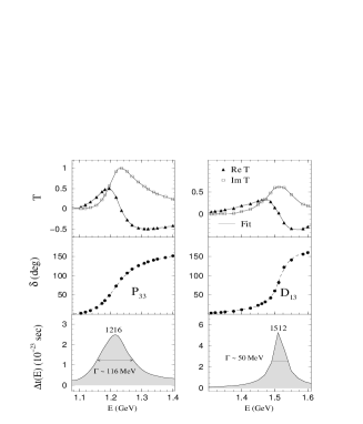
maximum can be read from Fig. 1 to be around 116 and 50 MeV respectively. The peaks in the energy distributions occur at 1216 and 1512 MeV respectively. The average values of Breit-Wigner masses (widths) given in the Summary Table (ST) of the Particle Data Group [41] for these $P_{33}$ and $D_{13}$ resonances are 1232 (120) and 1520 (120) MeV respectively. The $\Delta$(1232) decays almost 100% to the $\pi N$ channel and hence the time delay width seems to be in good agreement with the above value listed in the ST. The $D_{13}$ has a branching ratio of 50 to 60% to the $\pi N$ channel and the width of the time delay distribution is consistent with the partial width listed in the ST. Thus we see that in the case of purely elastic scattering as well as in the case of elastic scattering in the presence of inelastic channels, the method is quite useful. The peak position and width of the time delay distribution give the mass and elastic partial width of the resonance, respectively.

Interestingly, the $P_{33}$ phase shift of the only $\pi N$ resonance ($\Delta(1232)$) in the elastic region, remains positive and shows the characteristic resonant jump in this region. Hence, in this case, the speed defined in [50] is the same as time delay up to a constant factor.

3.1 New resonances from single energy values of phase shifts

We shall now evaluate time delay from fits to single energy (SE) values of phase shifts. Since the results depend crucially on the quality of the data, we chose data sets with small error bars and made separate $n^{th}$ order polynomial fits to different energy regions of the phase shift. It would be more appropriate to consider error bars and perform a $\chi^{2}$ fit, with a certain function. However, such a procedure would not be able to pick up the small structures and would amount to giving results similar to the energy dependent ones. We also chose to fit SE values of phase shifts rather than the SE values of real and imaginary parts of the $T$-matrix, simply as a matter of convenience. The time delay evaluated using fits to phase shifts or $T$-matrices is actually the same. The advantage of calculating time delay from such fits is that the results are directly related to data. The disadvantage is that they are sensitive to the quality of the data and hence to the fit. There also exists the well known continuum ambiguity problem with the SE values of phase shifts [58]. However, the present work does not aim at finding solutions to the problems related to the extraction of SE values. Hence, we use the values as available in literature and check if we still get some useful results for time delay.

We perform this analysis for the $I=1/2$ partial waves, $P_{11}$, $P_{13}$, $D_{13}$, $S_{11}$ and $F_{15}$ in $\pi N$ elastic scattering. We note that in spite of the above mentioned problems, we get strikingly similar peak positions and widths as compared to the Summary Table resonance parameters.

Figure 2: Single energy values of phase shifts and the corresponding time delay in the $S_{11}$ partial wave evaluated from a smooth fit to the phase shifts.

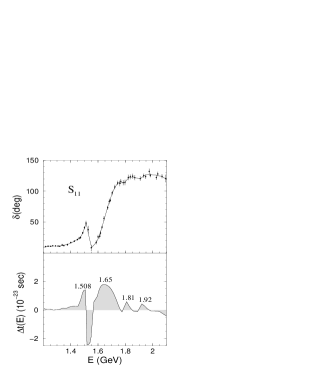
The results in Figs 2 and 3 reveal that time delay has the following main characteristics: (i) it locates well established resonances (ii) the positive peaks are more prominent than in the case where we calculated the same quantity for the energy-dependent solutions (see section 3.2 below), (iii) there exist regions of negative time delay in addition to the positive peaks (iv) the new feature here is that we find additional resonant peaks. At present, given the quality of the data, it is not clear if these new structures are artifacts of the fit to the data or genuine indications of (new) resonances. For example, in the $P_{11}$ and $S_{11}$ cases, we have hints for new resonances in the higher energy regions where the quality of data is worse. On the other hand, some one-star resonances like $P_{11}(2100)$ and $S_{11}(2090)$ are not excluded. We find evidence for the 3-star resonances $F_{15}(2000)$ and $P_{13}(1900)$, with some indication that the latter consists actually of two nearby resonances. In the $D_{13}$ partial wave, we observe distinct peaks at 1512, 1695 and 1940 MeV, which could be associated with the 4-, 3- and 2-star resonances $N(1520)$, $N(1700)$ and $N(2080)$ respectively. Note however that the existence of the two small peaks in this case depends crucially on two data points, and hence on the fit. These two points are sufficiently above continuum to justify the peaks (more so as they can be associated with known resonances). There seems to be more structure in the $1400-1700$ MeV region of $S_{11}$. A fit made to this detailed structure reveals the possibility of four resonances around $1650$ MeV. Indeed, there is some support for this structure from recent works in literature [5, 59], where the existence of new resonances at 1.6 and 1.7 GeV is predicted within quark models.

With the availability of more precise data on cross sections which would enable a better extraction of the

Figure 3: Single energy values of phase shifts and the corresponding time delay in the $P_{11}$, $P_{13}$, $D_{13}$ and $F_{15}$ partial waves of $\pi N$ elastic scattering. The time delay is evaluated using the solid lines which are fits to the single energy values of phase shifts.

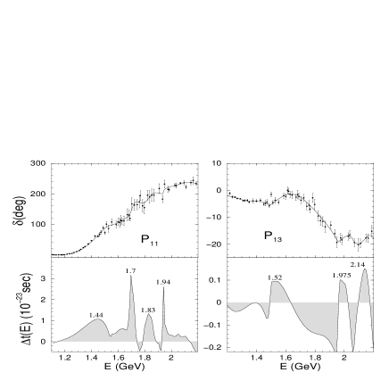
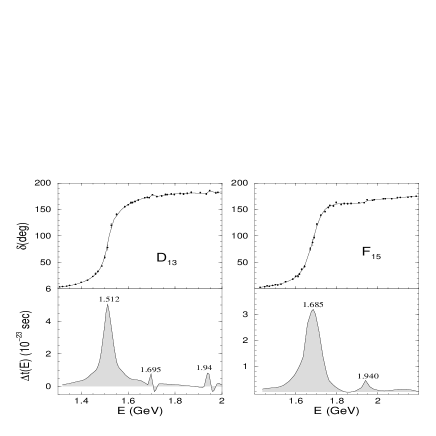
Table 1. Peak positions and corresponding widths from time delay plots using fits to single energy values of phase shifts. Masses and widths are in MeV.

L2I,2J	ST average	B.F.=$\Gamma_{\pi N}/\Gamma$	Partial width	Time Delay
Massstatus(Full	Pole (P)	(ST average)	= B.F.$\times$	Peak [Partial
Width)	Re P [-2 Im P]		(-2 Im P)	Widths]
D13
1520∗∗∗∗ [120]	1510 [115]	0.5 - 0.6	58 - 69	1512 [48]
1700∗∗∗ [100]	1680 [100]	0.05 - 0.15	5 - 15	1695 [12]
2080∗∗ [-]	1824 - 2120	-		1940 [18]
F15
1680∗∗∗∗ [130]	1670 [120]	0.6 - 0.7	72 - 84	1685 [91]
2000∗∗ [-]	-	-		1940 [33]
P11
1440∗∗∗∗ [350]	1365 [210]	0.6 - 0.7	126 - 147	1440 [207]
1710∗∗∗ [100]	1720 [230]	0.1 - 0.2	23 - 46	1700 [37]
-	-	-		1830 [65]
2100∗ [-]	-	-		1940 [13]
P13
-	-	-	-	1520 [101]
1900∗∗ [-]		-	-	1975 [51]
-	-	-	-	2140 [54]
S11
1535∗∗∗∗ [150]	1505 [170]	0.35 - 0.55	60 - 94	1510 [37.8]
-	-	-		1590 [25.2]
1650∗∗∗∗ [150]	1660 [160]	0.6 - 0.8	96 - 128	1630 [$\sim$ 40]
-	-	-		1680 [$\sim$ 24]
-	-	-		1700 [25.6]
-	-	-		1810 [31]
2090∗ [-]	1795 - 2220	-		1920 [38]

SE values of phase shifts, one could locate the resonances from time delay plots more accurately. We limit the discussion in this section only to the 5 partial waves shown in Figs 2 and 3, since a detailed analysis with all partial waves would make sense only when the SE values of phase shifts would be better known. We list our findings in Table 1.

3.2 Time delay from energy-dependent amplitudes

One of the standard methods of characterizing resonances involves locating the poles of an energy dependent $T$-matrix on the unphysical sheet. If these poles correspond to resonances, a positive maximum in time delay at the energies where the poles occur is expected. However, none of the existing analyses are constrained by this necessary condition. In what follows, we use the energy-dependent solutions obtained from the SAID program [56] as an example of such analyses, to evaluate time delay. We start with the $I=1/2$ partial waves in $\pi N$ elastic scattering. In Fig. 4a, we plot the SAID solution FA02 of the complex amplitudes. The corresponding time delay, using these $T$-matrices and those from an earlier analysis (SM95 solutions) by the same group, is plotted in Fig. 4b. The two solutions give rise to similar values of time delay in all except the $P_{11}$ and $P_{13}$ partial waves, where the peak positions differ. The FA02 solutions which are in better agreement with the SE values as compared to SM95 were obtained [60] using a much bigger database. The $P_{11}(~{}2000)$ peak obtained using SM95 is not seen with FA02. Indeed it was noted in [60], that the most significant shifts in the pole values occur in the P-waves ($P_{11}$ and $P_{13}$). We observe the resonant peaks in the $P_{11}$, $S_{11}$, $D_{13}$, $D_{15}$, $F_{15}$ and $P_{13}$ partial waves close to the pole positions predicted by the $T$-matrices. However, small peaks in the $G_{17}$ and $H_{19}$ partial waves appear at much lower values than the poles. The shifts in the time delay peaks as compared to the pole values could be due to the presence of a non-resonant background in these partial waves. Yet another explanation is offered in section 4. We give a more detailed discussion of the resonances in various partial waves now.

${\rm P}_{11}$-resonances: The SM95 solution gives a broad peak around $1400-1500$ MeV and a prominent peak at $\sim 2050$ MeV which could be attributed to the $P_{11}(1440)$ and the less established $P_{11}(2100)$ respectively. With the FA02, the two peaks at $1370$ MeV and $1745$ MeV are a clear signal of $P_{11}(1440)$ and $P_{11}(1710)$ listed in the ST. The FA02 $T$-matrix has two closely located poles at 1357 and 1386 MeV. The broad time delay peak around 1370 could actually be due to two closely overlapping resonances. The observation of the time delay peak at 1370 MeV which is much lower than the ST value of 1440 MeV is similar to the finding of Ref. [57]. In fact, most of the time delay peaks being close to the pole positions, occur at lower values than the parameters of the ST. The prominent peak at 2050 MeV with SM95 is not present in FA02 anymore.

We also note that $P_{11}$ resonances at 1500 and 1700 MeV were found in [61] from fits to the energy dependence of the amplitude obtained from an older VPI single energy analysis.

${\rm P}_{13}$-resonances: We see peaks at $1585$ and $1600$ MeV corresponding to the FA02 and SM95 solutions respectively. There exists a pole of the SM95 solution at $1717$ MeV which is close to the resonance $P_{13}(1720)$. However the FA02 pole occurs at a much lower value of $1584$ MeV. Though the pole values of the two solutions differ a lot, the time delay peaks with the two solutions are quite close.

${\rm S}_{11}$-resonances: We observe a positive peak around $1494$ MeV, which can be attributed to $S_{11}(1535)$, again as in the case of $P_{11}(1440)$ at a considerably lower value. The positive peak at $1650$ MeV is a nice manifestation of $S_{11}(1650)$. We note another phenomenon which commonly occurs in time delay plots now. The small peak at 1494 MeV is followed by a large negative region (which, as emphasized before, cannot be associated with resonance formation). The negative time delay is associated with the opening up of new channels in $\pi N$ scattering and in fact, the minimum in the dip occurs at the energy corresponding to maximum inelasticity. The energy derivative of the phase shift (and hence time delay) is related through the Beth-Uhlenbeck formula to the change in density of states in the presence of interaction [52]. The negative time delay corresponds to situations where due to the interaction, the density of states is less than in the absence of interaction. This is exactly what happens when the inelastic channels open up and there is a loss of flux from the elastic channel, thus reducing the density of states due to interaction. A detailed discussion on this issue can be found in [37]. A repulsive non-resonant background could make an additional contribution to the negative time delay.

Figure 4: (a) Real (dashed lines) and imaginary (solid lines) parts of the $T$-matrix solutions FA02 [56] for isospin, $I=1/2$, partial waves. (b) The time delay (solid lines) evaluated using the $T$-matrix solutions FA02 (shown in (a)) and an earlier version SM95 (dashed lines) by the same group.

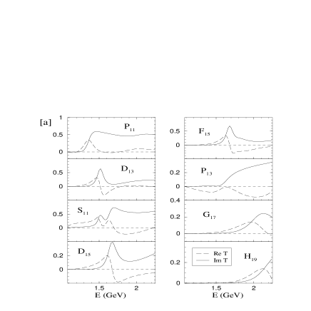
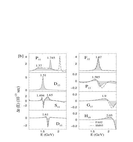
Table 2. Comparison of nucleon resonance parameters from time delay evaluated using the FA02 $T$-matrix solution, with the pole positions [62] of the same $T$-matrix, Summary Table values and Speed Plot poles (P = E - $i\Gamma/2$) .
L_2I,2J Speed Plot FA02 Branching Time delay Mass (Full - Pole(P) Pole (P) to $\pi$N Peak [Partial width) Re P [-2 Im P] Re P [-2 Im P] decay mode - width] P${}_{11}^{****}$ 1385 [164] 1357 [162] 60 - 70 $\%$ 1370 [298] 1440 (350) 1386 [170] $\dagger$ D${}_{13}^{****}$ 1510 [120] 1514 [103] 50 - 60 $\%$ 1510 [50] 1520 (120) S${}_{11}^{****}$ 1487 [ - ] 1516 [123] 35 - 55 $\%$ 1494 [48] 1535 (150) S${}_{11}^{****}$ 1670 [163] 1639 [155] 55 - 90 $\%$ 1650 [145] 1650 (150) D${}_{15}^{****}$ 1656 [126] 1664 [141] 40 - 50 $\%$ 1610 [93] 1675 (150) F${}_{15}^{****}$ 1673 [135] 1677 [121] 60 - 70 $\%$ 1670 [75] 1680 (130) 1778 [215] D${}_{13}^{***}$ 1700 [120] - 5 - 15 $\%$ - 1700 (100) P${}_{11}^{***}$ 1690 [200] - 10 - 20 $\%$ 1745 [50] 1710 (100) P${}_{13}^{***}$ 1686 [187] 1584 [287] 10 - 20 $\%$ 1585 [124] 1720 (150) P${}_{11}^{**}$ - 2009 [458] - - 2100 ( - ) G${}_{17}^{****}$ 2042 [482] 2084 [453] 10 - 20 $\%$ 1900 [310] 2190 (450) H${}_{19}^{****}$ 2135 [400] 2230 [553] 10 - 20 $\%$ 2050 [276] 2220 (400)

$\dagger$ Width is large due to the possibility of 2 overlapping resonances.

${\rm D}_{13}$ and ${\rm F}_{15}$-resonances: Time delay reveals the $D_{13}(1520)$ and ${\rm F}_{15}(1680)$ resonances. The three- and two-star resonances $D_{13}(1700)$ and $F_{15}(2000)$ respectively, do not appear in the time delay evaluated with the SM95 or FA02 solutions. This is consistent with the fact that the same solutions do not locate the corresponding poles. However, these two resonances do appear in the time delay plots obtained from fits to the single energy values of the $T$-matrix.

${\rm D}_{15}$ resonance: Though the peak is not prominent, its position and width are close to the pole values.

${\rm G}_{17}$ and ${\rm H}_{19}$-resonances: The peak positions in time delay are at much lower values as compared to the poles and much broader than the partial widths corresponding to the poles. It is not clear if such a large shift in these 2 cases should be attributed to the non-resonant background, since most of the other resonances were shifted from the pole values by only few tens of MeV at the most. Although a remote possibility, it could be that the shifted peaks represent resonances without corresponding poles and the poles at higher values do not correspond to resonances. These cases could be realistic examples similar to the constructed ones in [43], where the authors doubt the one-to-one correspondence between an unstable state and $S$-matrix pole. A good knowledge of the non-resonant background would clarify the situation. An alternative explanation will be given in section 4.

Figure 5: (a) Real (dashed lines) and imaginary (solid lines) parts of the $T$-matrix solutions FA02 [56] for isospin, $I=3/2$, partial waves. (b) The time delay evaluated using the $T$-matrix solutions FA02 (shown in (a)) and an earlier version SM95 by the same group.

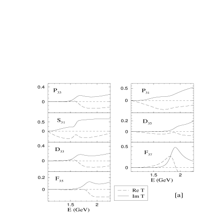
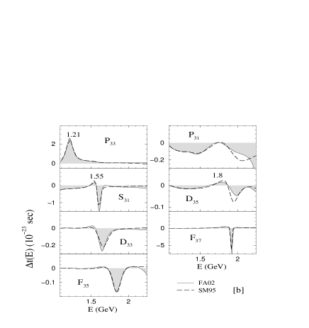
Table 3. Comparison of $\Delta$ resonance parameters from time delay evaluated using the FA02 $T$-matrix solution, with the pole positions [62] of the same $T$-matrix, Summary Table values and Speed Plot poles (P = E - $i\Gamma/2$).
L_2I,2J Speed plots FA02 Branching Time delay Mass (Full - Pole (P) Pole (P) to $\pi$N Peak [Partial width) Re P [-2 Im P] Re P [-2 Im P] decay mode - width] P${}_{33}^{****}$ 1209 [100] 1211 [101] $\geq$ 99 $\%$ 1210 [108] 1232 (120) P${}_{33}^{***}$ 1550 [ - ] - 10 - 25 $\%$ - 1600 (350) S${}_{31}^{****}$ 1608 [116] 1594 [114] 20 - 30 $\%$ 1550 [54] 1620 (150) D${}_{33}^{****}$ 1651 [159] 1633 [254] 10 - 20 $\%$ $\dagger$ 1700 (300) S${}_{31}^{***}$ 1780 [ - ] - 10 - 30 $\%$ - 1900 (200) F${}_{35}^{****}$ 1829 [303] 1832 [239] 5 - 15 $\%$ $\dagger$ 1905 (350) P${}_{31}^{****}$ 1874 [283] 1781 [493] 15 - 30 $\%$ - 1910 (250) P${}_{33}^{***}$ 1900 [ - ] - - - 1920 (200) D${}_{35}^{****}$ 1850 [180] 1918 [277] 10 - 20 $\%$ 1800 [157] 1930 (350) F${}_{37}^{****}$ 1878 [230] 1871 [236] 35 - 40 $\%$ $\dagger$ 1950 (300)

$\dagger$ Resonance signal not very clear

A comparison of the time delay peaks (evaluated using the FA02 solution) with the ST values and pole positions of FA02 and Speed Plots is given in Table 2. The branching fractions of the various resonances to the $\pi N$ decay channel are also listed. The widths in time delay are the partial widths corresponding to the $\pi N$ decay mode. Widths listed in the second and third columns are full widths. It can be seen that we get distinct resonance signals even for resonances with a branching fraction as small as 10-20 % to the $\pi N$ channel.

Next, we move on to the analysis of the $I=3/2$ partial waves in $\pi N$ scattering (Fig. 5). Many conventional pole positions of the energy-dependent $T$-matrices occur in regions of negative time delay. However, the time delay plots made from fits to the single energy values of the amplitude do show small peaks due to the $\Delta$ resonances with a small branching fraction to the $\pi N$ decay mode [37]. With the exception of $P_{31}$ where we do not find any positive region, the overall picture is similar to the case of the $I=1/2$ resonances. It is however fair to say that in the cases of $D_{33}$, $F_{35}$ and $F_{37}$ partial waves, the positive peaks are really too tiny to be conclusive. A comparison of the time delay peaks in the $I=3/2$ partial waves (evaluated using the FA02 solution) with the Summary Table values and pole positions of FA02 and Speed Plots is given in Table 3.

4 Time delay and Breit-Wigner amplitudes

In 2.2, we evaluated the time delay from a simple Breit-Wigner (BW) amplitude, assuming that the branching ratio for the elastic channel under consideration is $1$. We discuss this topic at this point again as we wish to interpret the results of our time delay analysis using $T$-matrix solutions which involve BW-like functions.

Generalizing the case of the BW amplitude by considering an elastic channel $i$ with a branching ratio, $Br\equiv\Gamma_{i}/\Gamma$, smaller than one, we have

$$T={\Gamma_{i}/2\over E_{R}-E-i\Gamma/2}$$ (11)

from which, after taking into account that the $S$-matrix is $S=1+2iT=\eta e^{2i\delta}$, the phase shift $\delta$ can be calculated to be

$$\delta={1\over 2}\tan^{-1}\biggl{[}{\Gamma_{i}(E_{R}-E)\over(E_{R}-E)^{2}+\Gamma^{2}/4-\Gamma_{i}\Gamma/2}\biggr{]}\,.$$ (12)

The derivative of the phase shift taken at $E=E_{R}$ is,

$${d\delta\over dE}\biggr{|}_{E=E_{R}}={1\over\Gamma}{Br\over(Br-1/2)}\,.$$ (13)

From Eq. 13, we see that if $Br<1/2$, time delay at resonance is negative. The negative region around $E_{R}$ is a local negative minimum accompanied on two sides by local positive maxima. We refer to this phenomenon as ‘two-horn’ structure. We can either say that the time delay concept loses its meaning in resonance physics in channels with a branching ratio less than $1/2$, or, the simple Breit-Wigner is not an adequate description for a resonant amplitude; although for many purposes other than time delay, a reasonable approximation. Indeed, Eq. (11) lacks the threshold factor and energy dependent widths. The threshold should at least be implemented correctly by $\Gamma_{i}\to\Gamma_{i}[q(E)/q(E_{R})]^{2l+1}$ (see e.g. [63] and references therein), where $q$ is the momentum of one of the initial particles in the CM frame. This $\Gamma_{i}$ is not unique and can be modified [54]. Moreover, as noted in [54] the rest of the energy dependence can take many different forms (see [64] for the latest collection of such resonant amplitudes). Hence, any argument in connection with time delay relating the latter with a Breit-Wigner should not be based on (11). This is exactly what we have done by computing the time delay from $T$-matrix solutions which are based on a more sophisticated BW form [54]. Certainly in some cases, an almost ‘two-horn’ structure is visible and is reminiscent of a BW. However, not always should this fact be considered as a drawback for the time delay concept. Indeed, in spite of an almost ‘two-horn’ structure for $P_{13}$, we find a mass of $1585$ MeV as compared to the pole value of $1584$ MeV. The $S_{11}$ partial wave, in spite of the almost ‘two-horn’ structure, displays two bona fide resonances at their expected values. This shows that a more sophisticated BW can indeed account for resonances in the time delay. The $D_{15}$, $S_{31}$ and $D_{35}$ resonances are in agreement with the values found in [54]. We do find the $P_{11}(1710)$ in spite of a branching ratio of $10-20\%$. Hence, this again demonstrates that arguments based on (11) are not at all stringent.

There are certainly problematic cases such as the $D_{33}$, $F_{37}$ and $F_{35}$. Dismissing the concept of time delay on account of these cases would amount to the same as dismissing the solutions of [54] which also fail to find several important resonances quoted in PDG (in addition to the fact that the resonance parameters do not always agree with the mean PDG value). This is clearly unacceptable as it is rather the rule than exception that different analyses in hadronic resonances yield different results. The fact that time delay is indecisive in certain cases could be due to the BW used in the parametrization of the $T$-matrix solutions. Although much better than (11) (as already proved by the time delay method itself), it might still not be the most general and suitable form for broad resonances [65]. In the $i\to j$ channel, the numerator of the BW amplitude gets replaced by $c_{i}c_{j}$ with $c_{i}=\sqrt{\Gamma_{i}/\Gamma}$. It was noted in [66] in connection with $\pi\pi$ scattering, that in order to obtain the correct $S$-matrix, the $c_{i}$’s should be complex. This should apply equally well to the baryon resonances (a similar argument can be found in [12]). It is worth noting that in our time delay analysis of meson-meson scattering [39], in all cases with $Br\ll 1/2$ for the elastic channel we found positive peaks (and no ‘two-horn’ structures). These cases are not isolated as there are six of them. Hence in contrast to the simple theoretical example of an oversimplified BW, in reality (at least for the meson-meson case) time delay works. We therefore suspect that an improvement on the BW in the baryon case will also lead to an improvement of the corresponding time delay results.

Finally, we also examine the influence of the non-resonant background using the BW parametrization for coupled channels as in [67]. Assuming a diagonal background, the $S$-matrix for elastic scattering ($i=j$) is given as,

$$S=e^{2i\eta_{i}}\biggl{[}1-2i{E_{R}\Gamma_{i}(E)\over E^{2}-E_{R}^{2}+iE_{R}\Gamma(E)}\biggr{]}$$ (14)

where $\eta_{i}$ is the background phase. In this case,

$${d\delta\over dE}\biggr{|}_{E=E_{R}}={Br\over\Gamma(E_{R})(Br-1/2)}+{d\eta_{i}\over dE}\biggr{|}_{E=E_{R}}$$ (15)

which generalizes Eq. (13).

5 Summary

Though the resonances in $\pi N$ scattering belong to one of the oldest topics of particle and nuclear physics, their study is far from being complete. This can be seen alone from their classification into four-, three-, two-, and one-star resonances according to the status of being well or less established. Disagreements in the extractions of resonance parameters are often encountered and theoretical model calculations sometimes predict new resonances.

Motivated by statements in literature that a positive time delay is a necessary condition to confirm a resonance, in the present work we have put the time delay method to test and have presented a systematic survey of time delay plots for the $\pi N$ resonances. In case of a clear signal, the resonance parameters could be extracted from the time delay plots. When $\Delta t(E)$ was calculated from the $T$-matrix solutions, we did not always find resonances at the energies corresponding to the poles of the $T$-matrix. This might be due to the model dependence of the $T$-matrix solutions or the non-resonant background in them. The calculation of $\Delta t(E)$ directly from data via phase shifts also characterized several established resonances. The results indicate that in some cases a known resonance could actually be a mixture of two neighbouring resonances. Detailed fits to the structure in the data revealed new resonances. For example, in the much talked about $S_{11}$ partial wave [5, 59, 68] we found some new resonances with some of them in agreement with the predictions in literature [59]. We believe that given more precise data, the time delay approach to resonances would be a very useful tool to characterize resonances.

APPENDIX

We briefly discuss two concepts related to time delay. These were not used in the present work, but we include them to avoid confusion among different concepts.

Time delay is closely related to the lifetime matrix Q, defined by Smith [18]. This Q is related to the scattering matrix S as, ${\bf Q}=-i\hbar\,{\bf S}\,d{\bf S}^{{\dagger}}/dE\,.$ The average time delay can be defined as a weighted average of the delay times $\Delta t_{ij}$ and is the same as $Q_{ii}$. Since the particle has probability $|S_{ij}|^{2}$ of emerging in the $j^{th}$ channel, the average time delay for a particle injected in the $i^{th}$ channel is given as,

$$\langle\,\Delta t_{i}\,\rangle_{av} = \sum_{j}\,S_{ij}^{*}S_{ij}\,\Delta t_{ij}\,\,=\,Re\biggr{[}\,-i\hbar\,\sum_{j}S^{*}_{ij}\,{dS_{ij}\over dE}\biggr{]}\,\,=\,Q_{ii}\,.$$

Strictly speaking, equations (1), (6) and (10) represent a time “delay” due to interaction. One can also derive an expression [16] (quoted here for $J=0$):

$$T(a)=8\pi^{2}\hbar\int_{0}^{\infty}dE^{\prime}|A(E^{\prime},E)|^{2}\left\{2{d\delta\over dE^{\prime}}+2a-{\sin[2(\delta+k^{\prime}a)]\over k^{\prime}}\right\}\,,$$

which is interpreted as the time spent within the spherical interaction region of radius $a$ in the presence of interaction. Since the above equation can be rewritten as an integral over a probability, $T(a)$ is always positive definite in contrast to (1), (6) and (10).

We also note that yet another discussion of time delay in classical and quantum scattering theory can be found in [31].

Acknowledgements: The authors wish to thank R. A. Arndt for useful discussions and I. Strakovsky for providing the pole values of their $T$-matrix solutions.

References

- [1] H. L. Anderson, E. Fermi, E. A. Long and D. E. Nagle, Phys. Rev. 85 936 (1952).
- [2] V. D. Burkert, “ Status of the program at Jefferson Lab”, hep-ph/0210321.
- [3] R.S. Hayano, Nucl. Phys. A655 369 (1999).
- [4] N. Isgur and G. Karl, Phys. Rev. D18 4187 (1978); ibid D20 1191 (1979); S. Godfrey and N. Isgur, Phys. Rev. D32 189 (1985); S. Capstick and N. Isgur, Phys. Rev. D34 2809 (1986); M. Kirchbach, M. Moshinsky and Yu. F. Smirnov, Phys. Rev. D64 114004 (2001).
- [5] B. Saghai and Z. Li, Proceedings of EMI 2002, Osaka, Ibaraki, Japan, eds. M. Fujiwara and T. Shima, World Scientific (2003), nucl-th/0202007; B. Saghai and Z. Li, Eur. Phys. J. A 11, 217 (2001); Z. Li and R. Workman, Phys. Rev. C 53, R549 (1996); B. Saghai and Z. Li, “ Beyond the known Resonances” nucl-th/03055004; M.M. Giannini, E. Santopinto and A. Vassallo, Eur. Phys. J. A12 447 (2001); ibid “Extra S11 and P13 in Hypercentral Constituent Model” nucl-th/0302019.
- [6] E. Hernandez, E. Oset and M. J. Vicente Vacas, Phys. Rev. C66 065201 (2002); J. E. Palomar and E. Oset, Nucl. Phys. A716 169 (2003); T. Inoue, E. Oset and M. J. Vicente Vacas, Phys. Rev. C65 035204 (2002); A. Ramos, A. Parreno, J. C. Nacher, E. Oset and C. Bennhold in Workshop of the Physics of Excited Nucleon, Mainz, Germany 2001, nucl-th/0106028; T. D. Cohen and L. Ya. Glozman, Phys. Rev. C65 016006 (2002); L. Ya. Glozman, Nucl. Phys. A663 252 (2000); W. Plessas, Few Body Systems Suppl. (2003) 1, nucl-th/0306021.
- [7] N. Kaiser, P. B. Siegel and W. Weise, Phys. Lett. B362, 23 (1995); Preprint nucl-th/9507036; Norbert Kaiser, P.B. Siegel and W. Weise, Nucl. Phys. A594, 325 (1995); Preprint nucl-th/9505043; P.B. Siegel and W. Weise (Regensburg U.), Phys. Rev. C38, 2221 (1988).
- [8] F. Close, Nature 389 230 (1997); G. S. Adams et al., Nucl. Phys. A680 335 (2000); S. U. Chung, Nucl. Phys. Proc. Suppl. 56 234 (1997); M. Gerber and M. Nowakowski, Nucl. Phys. A548 681 (1992).
- [9] L. Eisenbud, dissertation, Princeton, June 1948 (unpublished).
- [10] E. P. Wigner, Phys. Rev. 98, 145 (1955).
- [11] E. P. Wigner and L. Eisenbud, Phys. Rev. 72 29 (1947)
- [12] B. H. Bransden and R. Gordon Moorhouse, The Pion-Nucleon System (Princeton University Press, New Jersey, 1973).
- [13] M. L. Goldberger and K. M. Watson, Collision Theory (John Wiley, 1964); C. J. Joachain, Quantum Collision Theory (North-Holland, 1975); Quantum Mechanics, Arno Böhm, (Springer-Verlag, 1979); A. Messiah, Quantum Mechanics, V. I. North-Holland Publishing Company, Amsterdam, 1961.
- [14] J. R. Taylor, Scattering Theory: The Quantum theory on non-relativistic collisions, John Wiley and Sons, Inc., 1972.
- [15] D. Bohm, Quantum Theory (Prentice-Hall, New York, 1951).
- [16] H. M. Nussenzveig, Causality and Dispersion Relations, Academic Press, New York and London 1972.
- [17] A. I. Baz, Ya. B. Zel’dovich, A. M. Perelomov, “Scattering reactions and decay in non-relativistic quantum mechanics” (Israel Program of Scientific Translations, Jerusalem, 1969).
- [18] F. T. Smith, Phys. Rev. 118, 349 (1960); ibid Phys. Rev. 130 394 (1963).
- [19] N. R. Lipshutz, Phys. Rev. 181, 1972 (1969).
- [20] A. I. Baz, JETP 33, 923 (1957).
- [21] B. A. Lippmann, Phys. Rev. 151 1023 (1966).
- [22] M. L. Goldberger and K. M. Watson, Phys. Rev. 127 2284 (162).
- [23] M. Froissart, M. L. Goldberger and K. M. Watson, Phys. Rev. 131 2820 (1963).
- [24] R. Fong, Phys. Rev. 140 B762 (1965).
- [25] A. Peres, Ann. Phys. (N.Y.) 37 179 (1966).
- [26] J. M. Jauch and J. P. Marchand, Helv. Phys. Acta 40 217 (1967).
- [27] L. Calenza and W. Tobocman, Phys. Rev. 174 1115 (1968).
- [28] D. Bolle and T. A. Osborn, Phys. Rev. D11 3417 (1975).
- [29] H. M. Nussenzveig, Phys. Rev. D6 1534 (1972); ibid Phys. Rev. A55 1012 (1997).
- [30] J. O. Hirschfelder, Phys. Rev. A19 2463 (1979)
- [31] H. Narnhofer, Phys. Rev. D 22, 2387 (1980).
- [32] S. Bosnac, Phys. Rev. A24 777 (1981); ibid A30 153 (1984).
- [33] J. Fraxedas and J. Sesma, Phys. Rev. C37 2016 (1988); J. R. Pelaez, Phys. Rev. D 55 4193 (1997).
- [34] J. P. Svenne, T. A. Osborn, G. Pisent and D. Eyre, Phys. Rev. C40 1136 (1989).
- [35] P. Danielewicz and S. Pratt, Phys. Rev. C 53, 249 (1996); S. Leupold, Nucl. Phys. A 695, 377 (2001); C. David, C. Hartnack and J. Aichelin, Nucl. Phys. A 650, 358 (1999); A. B. Larionov et al., nucl-th/0107031.
- [36] G. Garcia-Calderon and J. Villavicencio, Phys. Rev. A66 032104 (2002).
- [37] N. G. Kelkar, J. Phys G: Nucl. Part. Phys. 29, L1 (2003); hep-ph/0205188.
- [38] N. G. Kelkar, M. Nowakowski and K. P. Khemchandani, J. Phys. G: Nucl. Part. Phys. 29 1001 (2003).
- [39] N. G. Kelkar, M. Nowakowski and K. P. Khemchandani, Nucl. Phys. A 724, 357 (2003).
- [40] Y. V. Fyodorov, H. J. Sommers, J. Math. Phys. 38 1918 (1997).
- [41] K. Hagiwara et al., (Particle Data Group), Phys. Rev. D 66, 010001 (2002) (URL:http://pdg.lbl.gov).
- [42] R. H. Dalitz and R. G. Moorhouse, Proc. Roy. Soc. Lond. A 318, 279 (1970).
- [43] G. Calucci, L. Fonda and G. C. Ghirardi, Phys. Rev. 166, 1719 (1968); G. Calucci and G. C. Ghirardi, Phys. Rev. 169 1339 (1968); L. Fonda, G. C. Ghirardi and G. L. Shaw, Phys. Rev. D8 353 (1973); L. Fonda, G. C. Ghirardi and A. Rimini, Rep. Prog. Phys. 41 587 (1978).
- [44] H. C. Ohanian and C. G. Ginsburg, Am. Journal of Phys. 42, 310 (1974).
- [45] R. G. Newton, Ann. of Phys. 14, 333 (1961).
- [46] J. S. Bell and C. J. Goebel, Phys. Rev. B 138, 1198 (1965).
- [47] P. D. B. Collins, R. C. Johnson and G. G. Ross, Phys. Rev. 176, 1952 (1968); N. Masuda, Phys. Rev. D1, 2565 (1970).
- [48] M. Nowakowski and A. Pilaftsis, Z. Phys. C60 121 (1993); M. Nowakowski, Int. J. Mod. Phys. A14 589 (1999).
- [49] A. Bianchini, R. J. Liotta and N. Sandulescu, Phys. Rev. C63, 024610 (2001).
- [50] G. Höhler, Newsletter 14, 168 (1998); ibid, Newsletter 9, 1 (1993).
- [51] Ken-Ichi Aoki, Atsushi Horikoshi, Etsuko Nakamura, Phys. Rev. A 62, 22101 (2000); J. G. Muga and C. R. Leavens, Phys. Rep. 338 353 (2000).
- [52] E. Beth and G. E. Uhlenbeck 1937 Physica 4 915; K. Huang 1963 Statistical Mechanics (Wiley, New York); R. K. Bhaduri, “Models of the nucleon: from quarks to soliton”, Lecture notes and supplements in physics: 22; Addison-Wesley publishing company, Inc. 1988; on pg. 29 is an example with discussion on resonances with the density of states formula; Z. Ahmed and S. R. Jain, “Number of quantal resonances”, quant-ph/0309206.
- [53] D. M. Manley and E. M. Saleski, Phys. Rev. D 45, 4002 (1992).
- [54] R. A. Arndt et al., Phys. Rev. C 52, 2120 (1995).
- [55] R. G. Sachs, Ann. Phys. (N.Y.) 22, 239 (1963).
- [56] Single energy values of phase shifts can be obtained from the SAID program made available on internet (URL: http://gwdac.phys.gwu.edu) by R. A. Arndt et al. To access it by telnet, link to gwdac.phys.gwu.edu with ‘LOGIN:said’. Password is not required.
- [57] G. Höhler, “Against Breit-Wigner parameters- a pole-emic” D. E. Groom et al., The European Physical Journal C 15, 1 (2000) and 1999 off-year partial update for the 2000 edition (URL: http://pdg.lbl.gov).
- [58] I. Saba-Stefanescu, Fortschritte der Physik 35, 573 (1987); J. E. Bowbock and H. Burkhardt, Rep. Prog. Phys. 38, 1099 (1975); D. Atkinson, M. de Roo and T. J. T. M. Polman, Phys. Lett. B 148, 361 (1984).
- [59] A. Svarc and S. Ceci, nucl-th/0009024; J. Z. Bai et al. (BES collaboration), Phys. Lett. B510 75 (2001); G.-Y. Chen, S. Kamalov, S.N. Yang, D. Drechsel and T. Tiator, nucl-th/0210013.
- [60] R. A. Arndt et al., nucl-th/0205067; nucl-th/9807087.
- [61] R. E. Cutkosky and S. Wang, Phys. Rev. D 42, 235 (1990).
- [62] R. A. Arndt, I. I. Strakovsky et al., private communication.
- [63] M. Nowakowski, Z. Phys. C35, 129 (1987).
- [64] H. Q. Zheng, “How to parameterize a light and broad resonance”, in International Symposium on Hadron Spectroscopy, Tokyo, Japan 24-26 Feb 2003, hep-ph/0304173.
- [65] Eef van Beveren and G. Rupp, Eur. J. Phys. C22, 493 (2001); ibid in Workshop on Recent Developments In Particle and Nuclear Physics, Coimbra, Portugal, 30 Apr 2001, hep-ph/0201006.
- [66] R. Kaminski, L. Lesniak and B. Loiseau, Eur. J. Phys. C9, 141 (1999)
- [67] A. M. Badalian, L. P. Kok, M. L. Polikarpov and Yu. A. Simonov, Phys. Rep. 82, 31 (1982); C. Garcia-Recio, J. Nieves, E. Ruiz Arriola and M. J. Vicente Vacas, Phys. Rev. D 67, 076009 (2003).
- [68] P. B. Siegel, S. Guertin, Newsletter 15, 246 (1999).