IFIC/02$-$14

FTUV/02$-$0822

Rho Meson Properties in the Chiral Theory Framework
J.J. Sanz-Cillero and  A. Pich

Departament de Física Teòrica, IFIC, Universitat de València - CSIC
Apt. Correus 22085, E-46071 València, Spain

We study the mass, width and couplings of the lightest resonance multiplet with $I\,(J^{PC})=1\,(1^{--})$ quantum numbers. Effective field theories based on chiral symmetry are employed in order to describe the form factor associated with the two-pseudoscalar matrix element of the QCD vector current. The bare poles of the intermediate resonances are regularized through a Dyson-Schwinger-like summation. We explore the role of the resonance width in physical observables and make a coupled-channel analysis of final-state interactions. This provides many interesting properties, as the pole mass $M_{\rho}^{\mbox{\tiny pole}}=764.1\pm 2.7\,{}^{+4.0}_{-2.5}$ MeV. At energies $E\mathrel{\hbox to0.0pt{\lower 4.0pt\hbox{\hskip 1.0pt$\sim$}\hss}\raise 1.0pt\hbox{$>$}}1$ GeV, a second $1\,(1^{--})$ resonance multiplet is considered in order to describe the data in a more consistent way. From the phenomenologically extracted resonance couplings, we obtain the chiral coupling $L_{9}^{r}(\mu_{0})=(7.04\pm 0.05\,{}^{+0.19}_{-0.27})\cdot 10^{-3}$, at $\mu_{0}=770$ MeV, and show how the running with the scale $\mu$ affects the resonance parameters. A $1/N_{C}$ counting is adopted in this work and the consistency of the large–$N_{C}$ expansion is tested. Finally, we make an estimation of the contribution from diagrams with resonances in crossed channels.

1 Introduction

It has become evident that Quantum Chromodynamics (QCD) is the correct theory which describes hadronic processes [1]. In the high-energy region ($E\gg 1$ GeV) the theory accepts a perturbative description and, accordingly, many calculations up to several orders in the perturbative expansion parameter $\alpha_{s}$ have been performed. These theoretical results have been successfully tested in many high-energy experiments. Nevertheless, since the running coupling constant $\alpha_{s}(\mu)$ increases as the energy decreases, the perturbative expansion in powers of $\alpha_{s}$ breaks down at energies $E\sim 1$ GeV. In this paper the problem of describing the $E\mathrel{\hbox to0.0pt{\lower 4.0pt\hbox{\hskip 1.0pt$\sim$}\hss}\raise 1.0pt\hbox{$<$}}1$ GeV region by employing effective theories of QCD [2, 3] will be analyzed.

When we study processes at energies much lower than the heavy quark masses, the degrees of freedom corresponding to heavy quarks decouple [4] and QCD, with only the light quark fields, yields a proper description. In the massless limit, the QCD lagrangian shows chiral symmetry: the left-handed and right-handed quark fields can be rotated independently under the $SU(n_{f})_{L}\otimes SU(n_{f})_{R}$ flavour chiral group, where $n_{f}$ is the number of light quarks. The symmetry is spontaneously broken to the $SU(n_{f})_{V}$ subgroup and $n_{f}^{2}-1$ massless Nambu-Goldstone bosons appear, associated with the broken generators. Nonetheless, as the light quark QCD lagrangian has small non-zero mass terms, chiral symmetry is also broken explicitly and the Nambu-Goldstone bosons gain small masses. These bosons have $J^{P}=0^{-}$ and are identified with the triplet of pions, in the $SU(2)$ case, and the ($\pi,\ K,\ \eta_{8}$) octet of light pseudoscalars for $SU(3)$.

The low-energy chiral effective field theory describing the dynamics of the lightest pseudoscalar multiplet was first developed for the $SU(2)_{L}\otimes SU(2)_{R}$ symmetry group [5], and was later generalized to the three flavour $SU(3)_{L}\otimes SU(3)_{R}$ case [6]. We will use the latter in order to include kaon interactions in our study. Chiral Perturbation Theory ($\chi$PT) [5, 6, 7, 8, 9] describes the physical low-energy amplitudes as an expansion in powers of quark masses and momenta over a characteristic chiral scale $\Lambda_{\chi}\simeq 4\pi f_{\pi}\sim 1$ GeV, with $f_{\pi}=92.4$ MeV the pion decay constant.

The expansion in powers of momenta over $\Lambda_{\chi}$ deteriorates as the energy of the process is increased and, in order to reach the relevant accuracy, one needs to add higher and higher chiral orders to the $\chi$PT lagrangian. In the resonance region one must introduce a different effective field theory with explicit massive fields to describe the degrees of freedom associated with the mesonic resonances. In the eighties, Gasser and Leutwyler worked out an $SU(2)_{L}\otimes SU(2)_{R}$ lagrangian describing the pions and the vector resonance $\rho(770)$ [5]. Later on this work was extended to the $n_{f}=3$ case [10], developing the Resonance Chiral Theory (R$\chi$T). Further studies on the R$\chi$T and $\chi$PT lagrangians constrained the resonance chiral couplings, employing the QCD short-distance behaviour of appropriate Green functions [11].

Once the resonance fields are explicitly included in the effective lagrangian, the chiral counting becomes ineffective because the masses of these resonances are of the same order than the chiral characteristic scale $\Lambda_{\chi}$. However, an expansion of QCD and its low-energy effective field theory in powers of $1/N_{C}$, with $N_{C}$ the number of quark colours, appears to be suitable [12]. In the large–$N_{C}$ limit, the hadronic description reduces to tree-level processes without hadron loops. As the $1/N_{C}$ expansion seems to yield a proper description of $N_{C}=3$  QCD, it seems also appropriate to expand the R$\chi$T results in powers of $1/N_{C}$ [13]. To a certain extent, this reduces to just counting the number of loops.

At leading order (LO) in $1/N_{C}$, R$\chi$T yields a good description of many phenomena. However it fails when the energy approaches the bare mass of a resonance. This situation is common to every unstable propagating state in a Quantum Field Theory when its propagator turns on-shell. It is solved by the Dyson-Schwinger summation of one particle insertion blocks (1PI), which provides the unstable particles with an imaginary absorptive part in the resonance propagator. This summation must also be done in R$\chi$T, with some prescriptions, but essentially in the same way. In Refs. [14, 15] the $\rho$-channel was studied and an appropriate off-shell width for the $\rho(770)$ resonance was obtained.

In this paper we continue the work put forward in Ref. [15], extending it to a coupled-channel analysis. We will study the vector form factor (VFF) [14, 15, 16, 17, 18] and overview the correlator of two QCD vector currents and the corresponding partial-wave scattering amplitude. It will be shown that our coupled-channel description of the resonance width agrees with the one in Ref. [15], obtained with a single-channel treatment. From the Dyson-Schwinger summation, we find that the rescattering dresses the bare propagator in a universal way. The induced correction only depends on the intermediate 1PI blocks and not on the final or initial states of the process.

We briefly describe the basic ingredients of the R$\chi$T effective action in Section 2. The Dyson-Schwinger analysis of the different observables is performed in Section 3. In Section 4 the obtained results are matched to the ${\cal O}(p^{4})$ $\chi$PT description and compared with the data in Section 5. The $\chi$PT coupling $L_{9}^{r}(\mu)$ is calculated here and a test of the $1/N_{C}$ expansion is also performed. The small corrections induced by resonance exchanges in the $t$–channel are estimated in Section 6. Our conclusions are finally given in Section 7. Some technical details have been relegated to the Appendices. In particular, a generalized formal summation of diagrams with two-body topologies is presented in Appendix C.

2 Resonance Chiral Theory

We will work with the $SU(3)$ octet of light pseudoscalar bosons, interacting through the ${\cal O}(p^{2})$ $\chi$PT lagrangian [6, 10]:

$$\mathcal{L}_{\mbox{\tiny$\chi$PT}}^{(2)}\;=\;\frac{\displaystyle f^{2}}{\displaystyle 4}\;\langle\,u^{\mu}u_{\mu}\,+\,\chi_{+}\,\rangle\,,$$ (1)

where $\langle\,...\,\rangle$ is short for the trace over flavour matrices and $f\approx f_{\pi}$ is the pion decay constant at lowest order. The tensors $u^{\mu}=i[u^{\dagger}(\partial^{\mu}-ir^{\mu})u-u(\partial^{\mu}-il^{\mu})u^{\dagger}]$ and $\chi_{+}=u^{\dagger}\chi u^{\dagger}+u\chi^{\dagger}u$ are functions of the left, right and scalar external sources $l^{\mu},\ r^{\mu}$ and $\chi$ [5, 6]. The pseudoscalar fields

$$\Phi=\left(\begin{array}[]{ccc}\frac{\pi^{0}}{\sqrt{2}}+\frac{\eta_{8}}{\sqrt{6}}&\pi^{+}&K^{+}\\ \pi^{-}&-\frac{\pi^{0}}{\sqrt{2}}+\frac{\eta_{8}}{\sqrt{6}}&K^{0}\\ K^{-}&\overline{K}^{0}&-\frac{2\eta_{8}}{\sqrt{6}}\end{array}\right)$$ (2)

are parameterized through the $SU(3)$ matrix  $u\equiv\exp{\left[\frac{i}{f\sqrt{2}}\,\Phi\right]}$.

The interactions of the Nambu-Goldstone bosons with the lightest multiplet of vector resonances

$$V_{\mu\nu}\,=\,\frac{\displaystyle\lambda^{a}}{\displaystyle\sqrt{2}}V_{\mu\nu}^{a}\,=\,\pmatrix{{1\over\sqrt{2}}\rho^{0}+{1\over\sqrt{6}}\omega_{8}+{1\over\sqrt{3}}\omega_{1}&\rho^{+}&K^{*+}\cr\rho^{-}&-{1\over\sqrt{2}}\rho^{0}+{1\over\sqrt{6}}\omega_{8}+{1\over\sqrt{3}}\omega_{1}&K^{\,*0}\cr K^{*-}&\bar{K}^{*0}&-{2\over\sqrt{6}}\omega_{8}+{1\over\sqrt{3}}\omega_{1}}_{\mu\nu}$$ (3)

are given by [10]

$$\mathcal{L}_{\mbox{\tiny R$\chi$T}}^{V}\,=\,\frac{\displaystyle F_{V}}{\displaystyle 2\sqrt{2}}\;\langle\,\ V_{\mu\nu}f_{+}^{\mu\nu}\,\rangle\,+\,i\;\frac{\displaystyle G_{V}}{\displaystyle\sqrt{2}}\;\langle\,V_{\mu\nu}u^{\mu}u^{\nu}\,\rangle\,,$$ (4)

where $f_{+}^{\mu\nu}=u\,F_{L}^{\mu\nu}u^{\dagger}+u^{\dagger}F_{R}^{\mu\nu}u$, with $F_{L,R}^{\mu\nu}$ the field strength tensors of the left and right external fields [5, 6]. We use the R$\chi$T lagrangian in the antisymmetric formalism provided in Ref. [10]. It was demonstrated in Ref. [11] that this antisymmetric description of the vector fields is equivalent to the more usual Proca formalism plus the ${\cal O}(p^{4})$ $\chi$PT lagrangian with its couplings $L_{i}$ constrained by the short-distance QCD behaviour.

In general, one should consider a set of vector resonance multiplets $V^{(i)}_{\mu\nu}$ with couplings $F_{V_{i}}$ and $G_{V_{i}}$. At low energies ($\sqrt{s}\mathrel{\hbox to0.0pt{\lower 4.0pt\hbox{\hskip 1.0pt$\sim$}\hss}\raise 1.0pt\hbox{$<$}}1.2$ GeV), the lightest multiplet yields the dominant contributions. However the tail of the second nonet may generate sizable corrections which must also be taken into account in the $\sqrt{s}\sim 1$ GeV region.

3 The Vector Form Factor

Let us consider the hadronic matrix element corresponding to the production of two pseudoscalars with $I=J=1$ through the charged $\bar{d}\,\gamma^{\mu}u$ vector current:

$$\langle\,P^{-}(p_{1})\,P^{0}(p_{2})\,|\,\bar{d}\,\gamma^{\mu}u\,\,|0\rangle\;=\;\sqrt{2}\ \left(p_{1}-p_{2}\right)^{\mu}\ \mathcal{F}^{(P)}_{\phantom{0}}(q^{2})\,,$$ (5)

with $q=p_{1}+p_{2}$. The label $P$ denotes the pair of pseudoscalars which are produced in the final state, either $\pi^{-}\pi^{0}$ or $K^{-}K^{0}$. The Lorentz structure is fixed by current conservation in the isospin limit.

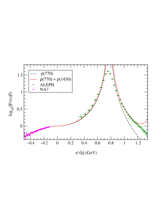
Figure 1: VFF at leading order in $1/N_{C}$ with one and two vector resonances. For the two-resonance case we have adopted the input parameters $M_{V_{1}}=775$ MeV, $M_{V_{2}}=1450$ MeV, $F_{V_{1}}G_{V_{1}}/f^{2}=1.1$ and $F_{V_{2}}G_{V_{2}}/f^{2}=-0.1$. Data from ALEPH [19] and NA7 [20].

At leading order in $1/N_{C}$, the vector form factor $\mathcal{F}^{(P)}_{0}(q^{2})$ is easily computed through the diagrams shown in Fig. 2(a). We put together the two $\mathcal{F}_{0}^{(P)}(q^{2})$ functions in the vector

$$\vec{\mathcal{F}}_{0}(q^{2})\;\equiv\;\left(\begin{array}[]{c}\mathcal{F}_{0}^{(\pi)}(q^{2})\\ \mathcal{F}_{0}^{(K)}(q^{2})\end{array}\right)\;=\;\left\{1\,+\,\sum_{i}\;\frac{F_{V_{i}}G_{V_{i}}}{f^{2}}\;\frac{\displaystyle q^{2}}{\displaystyle M_{V_{i}}^{2}-q^{2}}\right\}\ \left(\begin{array}[]{c}1\\ -\frac{1}{\sqrt{2}}\end{array}\right)\,.$$ (6)

The requirement that the vector form factor should vanish at infinite momentum transfer constrains the resonance couplings at LO in $1/N_{C}$ to satisfy the short-distance QCD relation [11, 13]

$$1\ -\ \sum_{i}\,\frac{F_{V_{i}}G_{V_{i}}}{f^{2}}\;=\;0\,.$$ (7)

If only one vector multiplet is considered, then $F_{V_{1}}G_{V_{1}}/f^{2}=1$ and one gets the familiar vector-meson dominance expression

$$\vec{\mathcal{F}}_{0}(q^{2})\;=\;\frac{\displaystyle M_{V_{1}}^{2}}{\displaystyle M_{V_{1}}^{2}-q^{2}}\ \left(\begin{array}[]{c}1\\ -\frac{1}{\sqrt{2}}\end{array}\right)\,.$$ (8)

This yields a rather good description of the data in the region $\sqrt{q^{2}}\mathrel{\hbox to0.0pt{\lower 4.0pt\hbox{\hskip 1.0pt$\sim$}\hss}\raise 1.0pt\hbox{$<$}}0.7$ GeV, below the $\rho(770)$ peak. Chiral loop corrections are subleading in the $1/N_{C}$ counting and turn out to be rather small in this case. Other resonances can also be included. The relevance of the large–$N_{C}$ expansion to approximate the physical vector form factor is clearly seen in Fig. 1, either with just one resonance or including a second multiplet.

The vector couplings are as well constrained in the large–$N_{C}$ limit by the relation

$$\sum_{i}\,\frac{\displaystyle 2\,F_{V_{i}}G_{V_{i}}-F_{V_{i}}^{2}}{\displaystyle M_{V_{i}}^{2}}\;=\;0\,,$$ (9)

provided by the short-distance QCD conditions over the axial form factor [11, 13].

For the simplest situation with a single resonance exchange, the short-distance QCD constraints yield $F_{V_{1}}=2\,G_{V_{1}}=\sqrt{2}\,f$ in the large–$N_{C}$ limit [11]. However, since we are going to work at higher orders in $1/N_{C}$, we will leave these couplings free and will test afterwards the deviation of their experimental values from the large–$N_{C}$ predictions, that we expect to be small.

3.1 Dyson-Schwinger Summation

Figure 2: Effective vertices for the vector current insertion producing two pseudoscalars (a) and for the two pseudoscalar scattering (b). The first terms come from $\mathcal{L}_{\mbox{\tiny$\chi$PT}}^{(2)}$ and the second ones from the interaction via an intermediate resonance due to the $\mathcal{L}_{\mbox{\tiny R$\chi$T}}^{V}$ lagrangian.

At energies close to the mass of a resonance we need to know the denominator of the resonance propagator beyond the leading, bare, order in $1/N_{C}$. What is usually done is a Dyson-Schwinger summation, as for instance in the QED photon polarization. That is, summing diagrams composed by a series of propagator, 1PI block, propagator, …, and so on. This summation regularizes the pole of the bare propagator. It gives a self-energy with its corresponding absorptive part, up to the perturbative order employed for the 1PI block. In R$\chi$T, however, at the same order than the resonance-exchange contribution there is also a local interaction from the $\mathcal{L}_{\mbox{\tiny$\chi$PT}}^{(2)}$ lagrangian. The Dyson-Schwinger summation must be then slightly modified. One constructs effective current vertices and effective scattering vertices [15], by adding the contribution from intermediate resonance exchanges in the $s$–channel to the local $\chi$PT interaction $\mathcal{L}_{\mbox{\tiny$\chi$PT}}^{(2)}$. Both contributions are of the same order in the $1/N_{C}$ counting. These effective vertices, shown in Fig. 2, are independent of the explicit formulation adopted for the spin–1 fields [11, 15]. If we use the Proca formulation we have to take into account the local interaction from the ${\cal O}(p^{4})$ $\chi$PT lagrangian as it is described in Ref. [11]. The inclusion of the local vertices is not important on the resonance peak but it turns to be relevant away from it.

For the moment, we are only interested in the imaginary part of the self-energy. Therefore, we will concentrate in the sum over diagrams with absorptive cuts. For the range of energies we are interested, the most relevant contributions come from intermediate states with two pseudoscalars; states with a higher number of particles being suppressed by phase space and chiral counting. Thus, we are going to sum diagrams constructed with an initial effective current insertion connected to an effective scattering vertex through a two-pseudoscalar loop. The pair of outgoing pseudoscalars from the scattering vertex are again connected to another effective scattering vertex through another two-pseudoscalar loop, and so on, as it can be seen in Fig. 3.

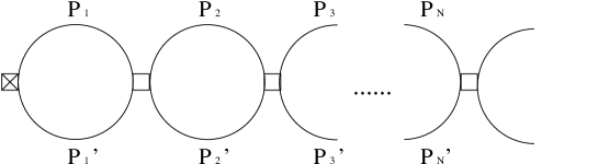
Figure 3: Diagrammatic summation at $N$ loops.

The off-shell effective current vertex shows the momentum structure

$$\vec{V}_{0}^{\mu}\;=\;\sqrt{2}\,\left[\ \vec{\mathcal{F}}_{0}\,P_{T}^{\mu\nu}\ +\ \vec{\mathcal{F}^{\prime}}_{0}\,P_{L}^{\mu\nu}\ \right]\ (p_{1}-p_{2})^{\nu}\,,$$ (10)

with $P_{T}^{\mu\nu}=g^{\mu\nu}-\frac{q^{\mu}q^{\nu}}{q^{2}}$ and $P_{L}^{\mu\nu}=\frac{q^{\mu}q^{\nu}}{q^{2}}$ the usual transverse and longitudinal Lorentz projectors. In the isospin limit, the second term with $\vec{\mathcal{F}^{\prime}}_{0}$ vanishes when the outgoing pseudoscalars are both on-shell. Notice that this off-shell function depends on the adopted parameterization of the fields, but the final on-shell amplitude does not depend on it.

When the current insertion $\vec{V}_{0}^{\mu}$ is connected to a successive number of loops and effective scattering vertices one gets $\vec{V}_{N}^{\mu}=\sqrt{2}\left[\vec{\mathcal{F}}_{N}P_{T}^{\mu\nu}+\vec{\mathcal{F}^{\prime}}_{N}P_{L}^{\mu\nu}\right](p_{1}-p_{2})^{\nu}$, where $N$ is the number of intermediate loops in the diagrammatic chain shown in Fig. 3. Thus the momentum structure remains. Inductively, from $N$ to $N+1$ loops we can observe the linear recurrence $\mathcal{F}_{N+1}^{(i)}=\sum_{j}\,\mathcal{M}^{ij}\,\mathcal{F}_{N}^{(j)}$, where $i=1$ stands for $\pi\pi$ and $i=2$ for $K\overline{K}$. This feature can be expressed in the matrix form

$$\vec{\mathcal{F}}_{N+1}\,=\,\mathcal{M}\;\vec{\mathcal{F}}_{N}\,=\,\mathcal{M}^{2}\;\vec{\mathcal{F}}_{N-1}\,=\,\cdots\,=\,\mathcal{M}^{N+1}\;\vec{\mathcal{F}}_{0}\,,$$ (11)

with $\vec{\mathcal{F}}_{N}$ the vector form factor at $N$ loops. The $2\times 2$ recurrence matrix takes the form

$$\mathcal{M}\ \ =\ -\ \Sigma^{-1}\,T_{\mbox{\tiny LO}}^{s}\,\Sigma^{-1}\ (192\,\pi\,B_{22})\,,$$ (12)

with the diagonal matrix $\Sigma=\$diag$\,\left(\sigma_{\pi},\ \sigma_{K}\right)$, being $\sigma_{P}=\sqrt{1-4\,m_{P}^{2}/q^{2}}$. The matrix

$$T_{\mbox{\tiny LO}}^{s}\;=\;\frac{\displaystyle q^{2}}{\displaystyle 96\pi f^{2}}\ \left\{\,1\,+\,\sum_{i}\;\frac{\displaystyle 2\,G_{V_{i}}^{2}}{\displaystyle f^{2}}\;\frac{\displaystyle q^{2}}{\displaystyle M_{V_{1}}^{2}-q^{2}}\,\right\}\;\;\Sigma\;\;\left(\begin{array}[]{cc}1&-\frac{1}{\sqrt{2}}\\[10.0pt] -\frac{1}{\sqrt{2}}&\frac{1}{2}\end{array}\right)\;\;\Sigma\,,$$ (13)

is the $s$–channel partial-wave scattering amplitude with $I=J=1$, at LO in $1/N_{C}$ [Fig. 2(b)]. The diagrams with resonances in the crossed channels produce a tiny contribution which will be taken into account in Section 6. We can also observe in Eq. (12) the diagonal matrix $B_{22}=\$diag$\,\left(B_{22}^{(\pi)},\ B_{22}^{(K)}\right)$, with the two-propagator Feynman integral $B_{22}^{(P)}$ given in Appendix A.

Summing the result in Eq. (11) for any number of loops, one gets a geometrical series which can be easily handled:

$$\vec{\mathcal{F}}\;=\;\sum_{N=0}^{\infty}\,\vec{\mathcal{F}}_{N}\;=\;\left(\sum_{N=0}^{\infty}\,\mathcal{M}^{N}\right)\;\vec{\mathcal{F}}_{0}\;=\;\left(1-\mathcal{M}\right)^{-1}\,\vec{\mathcal{F}}_{0}\;=\;\frac{\displaystyle 1}{\displaystyle 1-\mbox{tr}(\mathcal{M})}\;\vec{\mathcal{F}}_{0}\,.$$ (14)

The last identity is not trivial. The $\Sigma^{-1}T^{s}_{\mbox{\tiny LO}}\Sigma^{-1}$ matrix is proportional to a dimension-one projector and $\vec{\mathcal{F}}_{0}$ is eigenvector of this projector. Thus, $\mathcal{M}^{N}$ acting over $\vec{\mathcal{F}}_{0}$ reproduces again the vector $\vec{\mathcal{F}}_{0}$ times a number. The mathematical details can be found in Appendix B.

Afterwards a more complete calculation of the form factor will be developed. At the moment only the absorptive diagrams have been included and only the imaginary part is under control. Moreover, let us consider the simplest case of a single resonance exchange. The factor $\frac{1}{1-\mbox{tr}(\mathcal{M})}$ together with the initial $\vec{\mathcal{F}}_{0}$ generates a complex denominator $M_{V_{1}}^{2}-q^{2}-\xi(q^{2})$: a non-controlled real part plus a well defined imaginary term, given by

$$\mbox{Im}\ \xi(q^{2})\ \ =\ \ \mbox{Im}\ \xi_{\pi}(q^{2})+\mbox{Im}\ \xi_{K}(q^{2})\ .$$ (15)

The bubble loop summation provides an imaginary contribution which gets separate contributions from the $\pi\pi$ and $K\overline{K}$ channels. The corresponding partial widths are provided by

$$\mbox{Im}\ \xi_{P}(q^{2})\ =\ C_{P}\;\;\left(M_{V_{1}}^{2}\,-q^{2}+\frac{2\,G_{V_{1}}^{2}}{f^{2}}\,q^{2}\right)\frac{q^{2}\sigma_{P}^{3}}{96\,\pi\,f^{2}}\;\;\theta(q^{2}-4m_{P}^{2})\,,$$ (16)

with $C_{\pi}=1$ and $C_{K}=\frac{1}{2}$. When we substitute the coupling at LO in $1/N_{C}$, $G_{V_{1}}=f/\sqrt{2}$, these imaginary terms Im $\xi_{P}(q^{2})$ agree with the partial widths $M_{\rho}\Gamma_{\rho}^{(P)}(q^{2})$ obtained in Refs. [14, 15] from a simplified single-channel analysis. This energy dependence for the width was long ago considered by Gounaris and Sakurai from general arguments [22]. As well, they had exactly the same logarithm in their work that the one which naturally appears in our calculation of the absorptive contribution through the Feynman integral $B_{22}^{(P)}$.

The correlator of two vector currents and the $I=J=1$ partial-wave scattering amplitude, can be computed in a similar way. For the correlator we begin with a current effective vertex, like for the form factor, and connect it to a $N$-loop final-state interaction, which ends into another current effective vertex. For the scattering amplitude we start from a scattering effective vertex and go on connecting loops and scattering vertices in the same way. A similar rescattering effect appears in the three quantities. The resulting ($s$–channel) $I=J=1$ scattering amplitude takes the form:

$$T\ =\ \Sigma\left(\,\sum_{N=0}^{\infty}\;\mathcal{M}^{N}\right)\Sigma^{-1}\;T_{\mbox{\tiny LO}}^{s}\;=\;\Sigma\ \left(1-\mathcal{M}\right)^{-1}\Sigma^{-1}\;T^{s}_{\mbox{\tiny LO}}\;=\;\frac{\displaystyle 1}{\displaystyle 1-\mbox{tr}\{\mathcal{M}\}}\;\;T_{\mbox{\tiny LO}}^{s}\,.$$ (17)

The matrix structure $(1-\mathcal{M})^{-1}$ only depends on the scattering effective vertex and on the two-intermediate particle loop. As these are identical for the three quantities (VFF, correlator and scattering), the final-state interaction dresses the bare resonance pole in a universal way, providing the same complex pole for all processes.

4 Low-Energy Matching Conditions

All the former calculations must reproduce the QCD low-energy behaviour provided by the $\chi$PT framework. This allows to fix the polynomial ambiguities at a given order in the chiral expansion. We can identify the momentum expansion up to ${\cal O}(E^{4})$ of the resummed vector form factor (14) with the standard ${\cal O}(E^{4})$ $\chi$PT calculation in the usual $\overline{MS}-1$ scheme [23]. At leading order in $1/N_{C}$, we have the well-known relation [10, 13]

$$\left.L_{9}\right|_{N_{C}\to\infty}\;=\;\sum_{i}\;{F_{V_{i}}G_{V_{i}}\over 2\,M_{V_{i}}^{2}}\,,$$ (18)

with $F_{V_{i}},\ G_{V_{i}}$ and $M_{V_{i}}$ the bare parameters of the R$\chi$T lagrangian.

Keeping $1/N_{C}$ corrections, the ${\cal O}(E^{4})$ matching determines the regularized function $B_{22}^{r,(P)}$, up to the considered chiral order, to be [14, 15, 16]

$$B_{22}^{r,(P)}\;=\;\frac{\displaystyle 1}{\displaystyle 192\pi^{2}}\left[\sigma_{P}^{3}\,\ln{\left(\frac{\sigma_{P}+1}{\sigma_{P}-1}\right)}+\ln{\left(\frac{m_{P}^{2}}{\mu^{2}}\right)}-\frac{\displaystyle 5}{\displaystyle 3}+\frac{\displaystyle 8\,m_{P}^{2}}{\displaystyle q^{2}}\right]-\frac{\displaystyle 2}{\displaystyle 3}\,\delta L_{9}^{r}(\mu)\,,$$ (19)

where  $\delta L_{9}^{r}(\mu)\equiv L_{9}^{r}(\mu)\,-\,\left.L_{9}\right|_{N_{C}\to\infty}$. The renormalization scale dependence of the ${\cal O}(E^{4})$ $\chi$PT coupling $L_{9}^{r}(\mu)$ cancels out with the term $\ln\left(m_{P}^{2}/\mu^{2}\right)$. The resulting vector form factor from (14) takes then the form

$$\begin{array}[]{ccl}\vec{\mathcal{F}}&=&\ \ \frac{\displaystyle 1+\sum_{i}\frac{F_{V_{i}}G_{V_{i}}}{f^{2}}\frac{q^{2}}{M_{V_{i}}^{2}-q^{2}}}{\displaystyle 1+\left(1+\sum_{i}\frac{2G_{V_{i}}^{2}}{f^{2}}\frac{q^{2}}{M_{V_{i}}^{2}-q^{2}}\right)\frac{2q^{2}}{f^{2}}\left[B_{22}^{r,(\pi)}+\frac{1}{2}B_{22}^{r,(K)}\right]}\ \left(\begin{array}[]{c}1\\ -\frac{1}{\sqrt{2}}\end{array}\right)\,.\end{array}$$ (20)

With the information obtained from the VFF we obtain as well the ($s$–channel) $I=J=1$ partial-wave scattering amplitude,

$$T\ \ =\ \ \frac{\displaystyle\frac{\displaystyle q^{2}}{\displaystyle 96\pi f^{2}}\left(1+\sum_{i}\frac{2G_{V_{i}}^{2}}{f^{2}}\frac{q^{2}}{M_{V_{i}}^{2}-q^{2}}\right)}{\displaystyle 1+\left(1+\sum_{i}\frac{2G_{V_{i}}^{2}}{f^{2}}\frac{q^{2}}{M_{V_{i}}^{2}-q^{2}}\right)\frac{2q^{2}}{f^{2}}\left[B_{22}^{r,(\pi)}+\frac{1}{2}B_{22}^{r,(K)}\right]}\left(\begin{array}[]{cc}\sigma_{\pi}^{2}&-\frac{\displaystyle\sigma_{\pi}\sigma_{K}}{\displaystyle\sqrt{2}}\\[10.0pt] -\frac{\displaystyle\sigma_{\pi}\sigma_{K}}{\displaystyle\sqrt{2}}&\frac{\displaystyle\sigma_{K}^{2}}{\displaystyle 2}\end{array}\right)\,,$$ (21)

with $B_{22}^{r,(P)}$ being the same than in the VFF due to the optical theorem.

4.1 Scale Running

When the low-energy matching was performed, the unfixed $\delta L^{r}_{9}(\mu)$ parameter was left. It appeared as an extra constant in $B_{22}^{r,(P)}$. This also pointed out an ambiguity in the election of the scale and in the renormalization scheme, usually $\overline{MS}-1$ but not the unique one. For simplicity we will analyze this feature in the single resonance case and with the leading values of the couplings, $F_{V_{1}}=\sqrt{2}f=2G_{V_{1}}$. In this situation the VFF, for instance, becomes

$$\begin{array}[]{ccl}\vec{\mathcal{F}}&=&\frac{\displaystyle M_{V_{1}}^{2}}{\displaystyle M_{V_{1}}^{2}-q^{2}+\frac{2M_{V_{1}}^{2}q^{2}}{f^{2}}\left(B_{22}^{r,(\pi)}+\frac{1}{2}B_{22}^{r,(K)}\right)}\ \left(\begin{array}[]{c}1\\ -\frac{1}{\sqrt{2}}\end{array}\right)\\ \\ &=&\frac{\displaystyle M_{V_{1}}^{2}(\mu)}{\displaystyle M_{V_{1}}^{2}(\mu)-q^{2}+\frac{2M_{V_{1}}^{2}(\mu)q^{2}}{f^{2}}\left.\left(B_{22}^{r,(\pi)}+\frac{1}{2}B_{22}^{r,(K)}\right)\right|_{\delta L^{r}_{9}(\mu)=0}\ +\ {\cal O}(q^{2}/N_{C}^{2})}\ \left(\begin{array}[]{c}1\\ -\frac{1}{\sqrt{2}}\end{array}\right)\,,\end{array}$$ (22)

where

$$M_{V_{1}}^{2}(\mu)=M_{V_{1}}^{2}\left(1-\frac{2\,\delta L^{r}_{9}(\mu)\,M_{V_{1}}^{2}}{f^{2}}\right)\,.$$ (23)

The second line in (22) is easily obtained by multiplying the numerator and denominator with the factor $(1-2\,\delta L^{r}_{9}(\mu)\,M_{V_{1}}^{2}/f^{2})$. After introducing this definition, $\delta L^{r}_{9}(\mu)$ shuffles from $B_{22}^{r,(P)}$ to the parameter $M_{V_{1}}^{2}(\mu)$. Thus instead of two independent constants, $\delta L^{r}_{9}(\mu)$ and $M_{V_{1}}^{2}$, we only have the combination $M_{V_{1}}^{2}(\mu)$ replacing everywhere the parameter $M_{V_{1}}^{2}$. The term $\delta L^{r}_{9}(\mu)$ disappears from $B_{22}^{r,(P)}$, hence leaving in the regularized Feynman integral an explicit dependence on $\mu$. Moreover, the use of $M_{V_{1}}^{2}(\mu)$ in (18) allows us to recover the whole value of the $\chi$PT running coupling

$$L^{r}_{9}(\mu)\ \ =\ \ \left.L^{r}_{9}\right|_{N_{C}\to\infty}+\delta L^{r}_{9}(\mu)\ \ \simeq\ \ \frac{\displaystyle f^{2}}{\displaystyle 2\,M_{V_{1}}^{2}(\mu)}\ \ ,$$ (24)

up to the considered order. Therefore the parameter $M_{V_{1}}^{2}(\mu)$ captures the right dependence of $L_{9}^{r}(\mu)$ on the renormalization scale. In our phenomenological analysis, we will adopt the usual reference value $\mu_{0}=770$ MeV. Later on we will perform numerical studies at different scales $\mu$ and will examine the corresponding values of $L_{9}^{r}(\mu)$ derived through (24). The prescription of eliminating $\delta L^{r}_{9}(\mu)$ from $B_{22}^{r,(P)}$ is assumed in the following.

When studying the experimental data, we will observe that the couplings $F_{V_{1}}$ and $G_{V_{1}}$ are not exactly the ones provided by the large–$N_{C}$ limit, but they have small deviations. These parameters suffer also slight variations when more than one resonance is taken into account. In that case, the scale dependence does not go in such a straightforward way to the parameter $M_{V_{1}}(\mu)$ as we have seen in (23), although the relation is still obeyed within a given accuracy. The other parameters are going to suffer very tiny modifications with the scale but, at the precision of our study, they remain like constants.

5 Phenomenology

We are going to analyze the experimental data for the vector form factor, which is much cleaner than the one from $\pi\pi$ scattering. The vector form factor can be experimentally tested in the photoproduction of pseudoscalars from $e^{+}e^{-}$ annihilation or in $\tau$ decay. Although there are many data from $e^{+}e^{-}$ [20, 24], we have decided not to consider them, as we have not taken into account the $\omega$–$\rho$ mixing. We have studied the $\tau\to\nu_{\tau}2\pi$ data from ALEPH [19], which provides a covariance matrix to account for experimental error correlations. Similar data from CLEO [25] and OPAL [26] are also available.

The range of validity up to which we will extend our fit is at most $\sqrt{q^{2}}\leq 1.2$ GeV. Beyond this energy, multiparticle channels become important. First we perform a fit to the modulus of the VFF (ALEPH data) with the $\rho(770)$ resonance only. This yields the parameter $M_{V_{1}}(\mu)$ and the couplings $F_{V_{1}}$ and $G_{V_{1}}$. We choose as matching scale $\mu_{0}=770$ MeV, take the pion decay constant $f=f_{\pi}=92.4$ MeV as an input, and fit the region $2\,m_{\pi}\leq\sqrt{s}\leq\Lambda_{\mbox{\tiny max}}=1.2$ GeV. We obtain the values shown in Table 1, with a $\chi^{2}/$dof$=24.8/25$. The corresponding VFF is shown in Fig. 4. In order to estimate the systematic errors, we have varied the chiral parameter $f$ in the interval $f=92.4\pm 1.0$ MeV and the final point of the fit $\Lambda_{\mbox{\tiny max}}$ between 1.0 and 1.2 GeV. All these effects yield a more conservative result with a broader error. The first error in Table 1 is the one provided by MINUIT [27], while the second is our estimated systematic uncertainty.

Besides the lagrangian parameter $M_{V_{1}}(\mu)$, we can determine the more usual “physical”  masses: the Breit-Wigner mass $M_{{}_{BW}}$ and the pole mass $M_{\rho}^{\mbox{\tiny pole}}$. The energy where the phase-shift $\phi_{\pi\pi}=\frac{\pi}{2}$ defines the Breit-Wigner mass $M_{{}_{BW}}$ and the corresponding width is given by $1/\Gamma_{{}_{BW}}=M_{{}_{BW}}\left.\frac{d\phi_{\pi\pi}}{ds}\right|_{s=M_{{}_{BW}}^{2}}$ [22]. The complex pole of the observables in the second Riemann sheet, $s^{\mbox{\tiny pole}}_{\rho}=(M^{\mbox{\tiny pole}}_{\rho}-i\,\Gamma^{\mbox{\tiny pole}}_{\rho}/2)^{2}$, defines the alternative pole parameters.

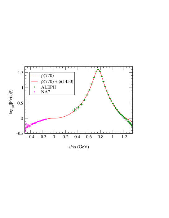
Figure 4: VFF fits to the $\tau\to\nu_{\tau}2\pi$ ALEPH data [19], with one and two $\rho$ resonances. Also shown are the $e^{+}e^{-}\to 2\pi$ data points from NA7 [20].

Chiral Coupling	$\rho(770)$	$\rho(770)\ +\ \rho(1450)$
$M_{V_{1}}(\mu_{0})$	$845.4\pm 1.1\,{}^{+0.8}_{-2.8}$ MeV	$839.4\pm 1.4\,{}^{+0.9}_{-2.3}$ MeV
$|F_{V_{1}}/f|$	$1.696\pm 0.008\,{}^{+0.010}_{-0.028}$	$1.669\pm 0.008\pm 0.017$
$|G_{V_{1}}/f|$	$0.695\pm 0.004\,{}^{+0.011}_{-0.019}$	$0.670\pm 0.005\,{}^{+0.012}_{-0.016}$
$F_{V_{1}}G_{V_{1}}/f^{2}$	$1.178\pm 0.010\,{}^{+0.009}_{-0.004}$	$1.119\pm 0.012\,{}^{+0.008}_{-0.018}$
$L_{9}^{r}(\mu_{0})=\sum_{i}\frac{F_{V_{i}}G_{V_{i}}}{2M_{V_{i}}^{2}(\mu_{0})}$	$(7.04\pm 0.05\,{}^{+0.19}_{-0.27})\cdot 10^{-3}$	$(6.79\pm 0.09\,{}^{+0.19}_{-0.27})\cdot 10^{-3}$
$M_{{}_{BW}}$	$776.0\pm 1.6\,{}^{+0.3}_{-0.7}$ MeV	$773.9\pm 2.0\,{}^{+0.3}_{-1.0}$ MeV
$\Gamma_{{}_{BW}}$	$156.2\pm 1.6\,{}^{+0.3}_{-3.0}$ MeV	$150.2\pm 2.0\,{}^{+0.7}_{-1.6}$ MeV
$M_{\rho}^{\mbox{\tiny pole}}$	$764.1\pm 2.7\,{}^{+4.0}_{-2.5}$ MeV	$770\pm 3\pm 3$ MeV
$\Gamma_{\rho}^{\mbox{\tiny pole}}$	$148.2\pm 1.9\,{}^{+1.7}_{-5.0}$ MeV	$137.3\pm 2.6\pm 2.6$ MeV

Table 1: Determination of some R$\chi$T and $\chi$PT couplings, at the scale $\mu_{0}=770$ MeV, from the VFF fit. The parameters $F_{V_{1}}/f$ and $G_{V_{1}}/f$ have the same sign as $F_{V_{1}}G_{V_{1}}/f^{2}>0$.

In Table 1 we have written the resulting values for these two different mass and width definitions. In order to derive those numbers, we have taken into account the correlations among the fitted parameters $M_{V_{1}}(\mu_{0})$, $F_{V_{1}}$ and $G_{V_{1}}$. Owing to the off-shell $q^{2}$ behaviour of the denominator, the pole mass turns out to be lower than the Breit-Wigner mass, in agreement with former works [28]. The opposite behaviour would have been obtained from a constant Breit-Wigner width parameterization.

In Fig. 5 we plot the phase-shift $\phi_{\pi\pi}$. In the low-energy region $\sqrt{s}\mathrel{\hbox to0.0pt{\lower 4.0pt\hbox{\hskip 1.0pt$\sim$}\hss}\raise 1.0pt\hbox{$<$}}0.7$ GeV, the experimental data appears to be slightly above the predicted values. The same behaviour can be observed in previous theoretical studies [14, 16, 17, 29, 30]. The experimental errors are probably underestimated in this region, although higher-order chiral corrections could induce small variations to our predictions. Other studies [28] seem to have a better control of the region closer to the $\pi\pi$ threshold and dominated by the $\chi$PT constraints. Beyond this region the agreement of our one-resonance analysis with the scattering data is good up to $\sqrt{q^{2}}\leq 1$ GeV. Above this point the prediction for the scattering amplitude begins to fail.

In order to better study the region around $\sqrt{s}\sim 1$ GeV, we include a second vector multiplet with the $\rho(1450)$. The effect of the tail of the $\rho(1450)$ can modify slightly the distribution in this region, where still the $\rho(770)$ dominates. Nonetheless, we cannot study energies much higher than $\sqrt{s}\sim 1.2$ GeV, since some not well-known strong inelasticities do arise (the experimental phase-shift data does not seem to pass through $3\pi/2$ at the $\rho(1450)$ mass [31]). Clearly, the two-pseudoscalar loops cannot incorporate all the inelasticity needed to describe the $\rho(1450)$ region. Other multiparticle intermediate states may be responsible for this large effect.

We have fitted our theoretical determination of the scattering amplitude with two resonances to the experimental phase-shift in the region $0.7$ GeV$\leq\sqrt{s}\leq 1.2$ GeV. The fit is not very sensitive to the $\rho(1450)$ mass, allowing a wide range of values. Nevertheless, it requires that $M_{V_{2}}(\mu_{0})\mathrel{\hbox to0.0pt{\lower 4.0pt\hbox{\hskip 1.0pt$\sim$}\hss}\raise 1.0pt\hbox{$>$}}1550$ MeV. Taking $M_{V_{2}}(\mu_{0})=1550$ MeV, the fit to the phase-shift gives $M_{V_{1}}(\mu_{0})=841.8\pm 0.6$ MeV,  $G_{V_{1}}/f=0.6631\pm 0.0027$ and $G_{V_{2}}/f=0.373\pm 0.028$, with $\chi^{2}/$dof$=18.8/22$. The fitted value of $G_{V_{2}}/f$ increases for larger masses of the $\rho(1450)$ resonance; the central value grows to 0.57 for $M_{V_{2}}(\mu_{0})=2000$ MeV. The precision of $G_{V_{1}}/f$ is improved, as expected, because the phase-shift has a larger sensitivity to this parameter. The differences between the analyses of $\phi_{\pi\pi}$ with one and two resonances are tiny for $\sqrt{s}\mathrel{\hbox to0.0pt{\lower 4.0pt\hbox{\hskip 1.0pt$\sim$}\hss}\raise 1.0pt\hbox{$<$}}1$ GeV. Beyond $\sqrt{s}\simeq 1.2$ GeV, the description breaks down because the pathological $\frac{\pi}{2}(2n+1)$ behaviour of the phase-shift in the neighbourhood of the $\rho(1450)$ still remains [see Fig. 5].

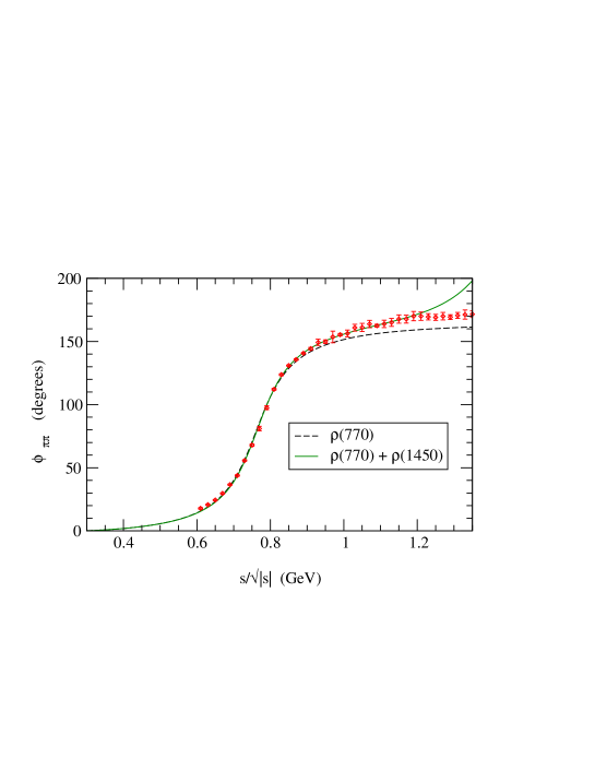
Figure 5: Phase-shift $\phi_{\pi\pi}$ of the $\pi\pi$ scattering amplitude. The parameters employed for the one-resonance graph are the same than in Fig. 4. The curve with two resonances takes the values from the fit to the scattering amplitude, with the inputs $M_{V_{2}}(\mu_{0})=1550$ MeV and $f=92.4$ MeV.

We have performed next another fit to the VFF ALEPH data, with two vector multiplets and taking $\Lambda_{\mbox{\tiny max}}=1.2$ GeV. Since in this region the data have very small sensitivity to the $\rho(1450)$ mass and the coupling $G_{V_{2}}$, we introduce as an input the value of $M_{V_{2}}(\mu_{0})$ and the corresponding coupling $G_{V_{2}}$ obtained from the phase-shift fit. The results of this VFF fit, given in Table 1, have a $\chi^{2}/$dof$=14.7/24$. The systematic errors have been estimated varying the pion decay constant in the interval $f=92.4\pm 1.0$ MeV and the value of $M_{V_{2}}(\mu_{0})$ in the range from $1550$ to $2000$ MeV, which implies $G_{V_{2}}/f=0.37\pm 0.03\,{}^{+0.2}_{-0.0}$. In this analysis we have recovered as well the Breit-Wigner and pole masses and widths for the $\rho(770)$ meson. We have not tried to determine the $\rho(1450)$ pole, because it would lie in a region which is not well described. We also give in Table 1 the $\chi$PT coupling $L_{9}^{r}(\mu_{0})$ at the matching scale $\mu_{0}=770$ MeV.

The VFF fit is sensitive to the product of couplings $F_{V_{2}}G_{V_{2}}/f^{2}$. One gets,

$$F_{V_{2}}G_{V_{2}}/f^{2}=0.007\pm 0.024\,{}^{+0.000}_{-0.050}\,.$$ (25)

For the range of $G_{V_{2}}/f$ values quoted before, this implies $F_{V_{2}}/f=0.02\pm 0.06\,{}^{+0.00}_{-0.08}$.

Modifications of the $\rho(1450)$ inputs produce sizable variations on the $\rho(770)$ couplings. Thus, a better knowledge of the $\rho(1450)$ is needed to get more accurate values of the $\rho(770)$ parameters from a two-resonance fit. The results are consistent with the more precise determinations from the fit with only one resonance, which we take as our best estimates.

5.1 Running of $L^{r}_{9}(\mu)$

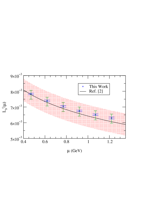
Figure 6: Comparison between the usually quoted value of the chiral coupling $L_{9}^{r}(\mu)$ [2] (shadowed band) and some determinations from the fit at several matching scales: $L_{9}^{r}(\mu)=\sum_{i}\frac{F_{V_{i}}G_{V_{i}}}{2M_{V_{i}}^{2}(\mu)}$. The smaller error intervals are the statistical uncertainties given by MINUIT, the larger ones indicate the total errors including systematic contributions.

We have seen in Section 4, from a simplified theoretical analysis, that the parameter $M_{V_{1}}(\mu)$ depends on the $\chi$PT renormalization scale adopted in the loop function $B_{22}^{r,(P)}$, in such a way that the physically measurable VFF is scale independent as it should. The dependence of $M_{V_{1}}(\mu)$ with the scale was given by the equation

$$M_{V_{1}}^{2}(\mu_{2})-M_{V_{1}}^{2}(\mu_{1})=\frac{M_{V_{1}}^{2}}{64\pi^{2}f^{2}}\ln{\left(\frac{\mu_{2}^{2}}{\mu_{1}^{2}}\right)}\,,$$ (26)

as $L_{9}^{r}(\mu_{2})-L_{9}^{r}(\mu_{1})=\delta L_{9}^{r}(\mu_{2})-\delta L_{9}^{r}(\mu_{1})=-\frac{1}{128\pi^{2}}\ln{\left(\frac{\mu_{2}^{2}}{\mu_{1}^{2}}\right)}$. The theoretical running of $M_{V_{1}}(\mu)$ induces a scale dependence on the predicted value of $L_{9}^{r}(\mu)$ in Eq. (24). When the phenomenological fit is performed at different values of $\mu$, the parameter $M_{V_{1}}(\mu)$ increases with $\mu$. The other parameters of the fit remain essentially unaffected, i.e. they suffer modifications much smaller than their errors. Varying the scale $\mu$ in the range between 0.5 GeV and 1.2 GeV, the $\chi^{2}$ varies less than $2\%$.

The fitted $L_{9}^{r}(\mu)$ results are compared in Fig. 6 to the usually quoted values [2]. At the standard reference scale $\mu_{0}=770$ MeV, we obtain

$$L_{9}^{r}(\mu_{0})=(7.04\pm 0.05\,{}^{+0.19}_{-0.27})\cdot 10^{-3}\,,$$ (27)

which improves considerably previous determinations [2, 33]. The systematic errors would increase to ${}^{+0.19}_{-0.50}$ if we would have considered the fit with two resonances. The lack of knowledge about the second multiplet parameters introduces an extra uncertainty of the same order than the one we have with only one resonance.

5.2 Large–$N_{C}$ relations

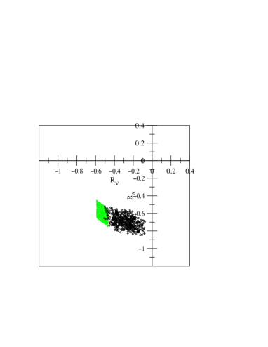
Figure 7: Allowed region in the $(R_{V},R_{A})$ plane. The shaded zone on the left corresponds to the one-resonance study, while the dotted zone results from the analysis with two resonances.

As we work at higher orders in $1/N_{C}$, our experimental results have next-to-leading deviations from the LO values provided by the two short-distance QCD relations (7) and (9). We are going to test now how well they are satisfied. Typically, there should be a deviation from zero of ${\cal O}(1/N_{C})$ in the VFF relation (with $N_{C}=3$ in physical QCD), as the leading terms of the left-hand side of the equalities are $F_{V_{1}}G_{V_{1}}/f^{2}\sim 1$. The deviation in the axial form factor constraint should be of ${\cal O}(1/N_{C})\cdot 0.03$, because its leading terms are $2F_{V_{1}}G_{V_{1}}/M_{V_{1}}^{2}\sim F^{2}_{V_{1}}/M_{V_{1}}^{2}\sim 0.03$.

In Fig. 7, we have plotted the variables

$$\begin{array}[]{ccl}R_{V}&\equiv&\displaystyle\left\{1-\sum_{i}\;\frac{\displaystyle F_{V_{i}}G_{V_{i}}}{\displaystyle f^{2}}\right\}\ \cdot\ N_{C}\ ,\\ \\ R_{A}&\equiv&\displaystyle\left\{\sum_{i}\;\frac{\displaystyle 2F_{V_{i}}G_{V_{i}}-F^{2}_{V_{i}}}{\displaystyle M_{V_{i}}^{2}}\right\}\ \cdot\ N_{C}\ (0.03)^{-1}\ ,\\ \end{array}$$ (28)

which have been normalized with appropriate factors so that the expected deviations from zero are of ${\cal O}(1)$. We have performed a scanning of the range of values for the R$\chi$T couplings obtained from the VFF fits. We can see in the figure that the separation from the large–$N_{C}$ QCD relations is indeed of the expected order for both types of fits (with one or two resonances). Thus, the short-distance relations (7) and (9) are well satisfied, within the given accuracy.

6 Uncertainties from Higher-Order Corrections

There exist many more diagrammatic contributions which have not been included in our results. We show in Appendix C that, when the production of multiparticle states is neglected, it is possible to define a generalized summation of Feynman diagrams with two-body topologies. It makes use of a kernel function $\mathcal{K}$, associated with the two-body scattering amplitude, which incorporates those contributions not included in our effective $s$–channel vertex of Fig. 2(b). The resulting VFF can be formally written in a very compact form, given in Eq. (C.10). Making a $1/N_{C}$ expansion of the kernel $\mathcal{K}$, one can easily check that our $s$–channel result in Eq. (14) corresponds to the leading-order approximation. The first correction originates from a single resonance exchange in the $t$–channel, which induces a subleading contribution of ${\cal O}(1/N_{C})$ to the kernel $\mathcal{K}$. The exchange of $n$ meson fields contributes to the kernel at ${\cal O}(1/N_{C}^{n})$.

A general calculation of those higher-order corrections is a formidable task. We know, however, that in the energy region we are studying the tree-level scattering in the $t$–channel is much smaller than the one coming from the $s$–channel, what seems to imply that they contribute as a small perturbation. To estimate the size of those corrections, we have analyzed the leading contribution from t–channel resonance exchange between the final pions. According to the results in Appendix C, it induces a multiplicative correction into the VFF:

$$\vec{\mathcal{F}}\;\approx\;\left[1-\mathcal{G}^{t}_{1R}\right]^{-1}\left[1+\Sigma^{-1}T^{s}_{\mbox{\tiny LO}}\,\Sigma^{-1}(192\pi B_{22}^{r})\right]^{-1}\vec{\mathcal{F}}_{0}\,,$$ (29)

where $\mathcal{G}^{t}_{1R}$ is the contribution from a single t–channel exchange.

The complete calculation of $\mathcal{G}^{t}_{1R}$ is rather involved, since it makes necessary to address the renormalization of R$\chi$T. This is a very interesting issue, which we plan to analyze in a future publication where a full analysis of the VFF at next-to-leading order in $1/N_{C}$ will be attempted. Here, we are only interested in its numerical impact on the results presented in the previous sections. For simplicity, we will study $\mathcal{G}^{t}_{1R}$ in the SU(2) theory; i.e. we neglect the tiny contributions from diagrams with kaons in the intermediate loop or in the final state ($\mathcal{G}^{t\ (\pi,K)}_{1R}=\mathcal{G}^{t\ (K,\pi)}_{1R}=\mathcal{G}^{t\ (K,K)}_{1R}=0$). Moreover, we will work in the chiral limit ($m_{\pi}=0$).

Although there are several Feynman diagrams contributing, we only need to consider the dominant one where the current vertex $(k_{1}^{\mu}-k_{2}^{\mu})$ produces a $\pi^{-}(k_{1})\pi^{0}(k_{2})$ pair, which is rescattered through a $t$–channel resonance. This diagram generates the interesting non-analytic contributions, plus a divergent local correction which should combine with the local contributions from the other diagrams to provide a physical finite result. Since we are interested in the region $\sqrt{s}\ll 2M_{V}$ (i.e. we work below the two-resonance cut), there are no additional sources of non-analytic terms. The local ambiguity can be fixed to ${\cal O}(E^{4})$ by matching Eq. (29) with the known $\chi$PT result. This requires $\mathcal{G}^{t}_{1R}\sim{\cal O}(E^{4})$. The exchange of a vector resonance can be easily computed in this way. One gets:

$$\begin{array}[]{ll}\mathcal{G}^{t\ (\pi,\pi)}_{1V}=&\frac{\displaystyle G_{V_{1}}^{2}\,M_{V_{1}}^{2}}{\displaystyle(4\pi)^{2}f^{4}}\left\{\left[\mbox{Li}_{2}\left(1+\frac{\displaystyle q^{2}}{\displaystyle M_{V_{1}}^{2}}\right)-\mbox{Li}_{2}\left(1\right)\right]\left(2\,\frac{\displaystyle M_{V_{1}}^{4}}{\displaystyle q^{4}}+5\,\frac{\displaystyle M_{V_{1}}^{2}}{\displaystyle q^{2}}+2\right)\right.\\ \\ &\qquad\quad\;\left.+\;\ln{\left(-\frac{\displaystyle q^{2}}{\displaystyle M_{V_{1}}^{2}}\right)}\left(2\,\frac{\displaystyle M_{V_{1}}^{2}}{\displaystyle q^{2}}+4+\frac{\displaystyle 1}{\displaystyle 6}\,\frac{\displaystyle q^{2}}{\displaystyle M_{V_{1}}^{2}}\right)-2\,\frac{\displaystyle M_{V_{1}}^{2}}{\displaystyle q^{2}}-\frac{\displaystyle 9}{\displaystyle 2}-\frac{\displaystyle 35}{\displaystyle 36}\,\frac{\displaystyle q^{2}}{\displaystyle M_{V_{1}}^{2}}\right\}\,.\end{array}$$ (30)

Since $\mathcal{G}^{t\ (\pi,\pi)}_{1V}\sim q^{4}/M_{V}^{2}$, we can neglect the exchange of higher-mass vector resonances. However, we will also consider the $t$–channel exchange of scalar resonances from the lightest multiplet, with a mass $M_{S}\simeq 1$ GeV [10, 32] and couplings $c_{d},c_{m}\simeq f/2$ [34]. It provides the contribution:

$$\begin{array}[]{ll}\mathcal{G}^{t\ (\pi,\pi)}_{1S}=&\frac{\displaystyle 2\,c_{d}^{2}\,M_{S}^{2}}{\displaystyle(4\pi)^{2}f^{4}}\left\{\left[\mbox{Li}_{2}\left(1+\frac{\displaystyle q^{2}}{\displaystyle M_{S}^{2}}\right)-\mbox{Li}_{2}\left(1\right)\right]\left(2\,\frac{\displaystyle M_{S}^{4}}{\displaystyle q^{4}}+\frac{\displaystyle M_{S}^{2}}{\displaystyle q^{2}}\right)\right.\\ \\ &\qquad\qquad\left.+\ln{\left(-\frac{\displaystyle q^{2}}{\displaystyle M_{S}^{2}}\right)}\left(2\,\frac{\displaystyle M_{S}^{2}}{\displaystyle q^{2}}+\frac{\displaystyle 1}{\displaystyle 6}\,\frac{\displaystyle q^{2}}{\displaystyle M_{S}^{2}}\right)-2\,\frac{\displaystyle M_{S}^{2}}{\displaystyle q^{2}}-\frac{\displaystyle 1}{\displaystyle 2}+\frac{\displaystyle 1}{\displaystyle 36}\,\frac{\displaystyle q^{2}}{\displaystyle M_{S}^{2}}\right\}\,.\end{array}$$ (31)

This result includes contributions from the singlet and the octet scalars.

At energies below and around the $\rho(770)$ peak, these $t$–channel diagrams give a correction smaller than $5\%$, which is within the uncertainties of the numerical analyses performed in the previous section. However, above $E\sim 1.2$ GeV the vector contribution becomes larger than 10% and these topologies cannot be neglected any more. This kind of diagrams turn out to be very important at high energies.

We have repeated our previous fits to the VFF ALEPH data, including the correction induced by $\mathcal{G}^{t\ (\pi,\pi)}_{1R}=\mathcal{G}^{t\ (\pi,\pi)}_{1V}+\mathcal{G}^{t\ (\pi,\pi)}_{1S}$. The results of these fits are compatible with the ones obtained before, showing that our former studies neglecting crossed channels provide a good description within the given precision.

7 Conclusions

A quantum field theory description of strong interactions at energies around the hadronization scale, $E\sim 1$ GeV, requires appropriate non-perturbative tools. While a fundamental understanding of the confinement region of QCD is still lacking, substantial phenomenological progress can be achieved through effective field theories incorporating the relevant symmetries and dynamical degrees of freedom.

Using an effective chiral lagrangian which includes pseudoscalars and explicit resonance fields, we have investigated the VFF and related $I=J=1$ observables in the interesting $E\sim 1$ GeV energy range. The heavy particles make the standard chiral counting in powers of momenta useless, because their masses are of the same order than the chiral symmetry breaking scale. Therefore, we have adopted instead the more convenient large–$N_{C}$ expansion, which provides a powerful tool to organize the calculation.

At the leading order in $1/N_{C}$, one gets an excellent description of the VFF, far away from the resonance singularities. A proper understanding of the zone close to the $\rho(770)$ pole, requires the inclusion of next-to-leading contributions providing the non-zero width of the unstable meson. The dressed propagator can be calculated through a Dyson-Schwinger summation of the dominant $s$–channel rescattering corrections, constructed from effective Goldstone vertices containing both the local $\chi$PT interaction and the resonance-exchange contributions [13, 14, 15, 16].

We have extended the Dyson-Schwinger summation of effective vertices to handle problems with coupled channels in a systematic way, through the recurrence matrix $\mathcal{M}$. The inverse matrix $\left(1-\mathcal{M}\right)^{-1}$, generated by final-state interactions, provides the right unitarity structure of the observables [17, 29, 30]. Moreover, with an $SU(3)$–symmetric dynamics (the vertices contain only derivatives and no quark masses), $\left(1-\mathcal{M}\right)^{-1}$ acts just like a pure number $\left[1-\mbox{tr}\{\mathcal{M}\}\right]^{-1}$. Hence, there is no mixing among loops and the total decay width is simply given by a sum of separate contributions from the different channels, which correspond to the partial decay widths. An improved diagrammatic summation of more general two-body topologies has been given in Appendix C. It includes the smaller $t$–channel corrections, through the $1/N_{C}$ expansion of a non-trivial interaction kernel $\mathcal{K}$ associated with the two-pseudoscalar scattering amplitude.

The Feynman loops fully determine the non-analytic contributions, which are dictated by unitarity and chiral symmetry. The local corrections, however, are functions of the theoretically unknown couplings of the effective lagrangian. They incorporate the short-distance dynamics and take care of the regularization and renormalization prescriptions adopted in the calculation. A significative reduction on the number of free parameters is obtained, requiring the different amplitudes to satisfy the appropriate QCD constraints at large momentum transfer [10, 11]. In fact, a very successful prediction of the most relevant $O(E^{4})$ $\chi$PT couplings is obtained, under the reasonable assumption that the lightest resonance multiplets give the dominant effects at low energies [13]. We have resolved the local ambiguities of the VFF, imposing the QCD short-distance constraints and performing a low-energy matching with the known ${\cal O}(E^{4})$ $\chi$PT result.

Working within the single-resonance approximation [13], we have obtained a good fit to the ALEPH $\tau\to\nu_{\tau}2\pi$ data [19], in the range $2m_{\pi}\leq\sqrt{q^{2}}\leq 1.2$ GeV. At the chiral renormalization scale $\mu_{0}=770$ MeV, the fit gives the values shown in Table 1 for the main $\rho$ parameters. The corresponding resonance pole $s^{\mbox{\tiny pole}}=(M^{\mbox{\tiny pole}}_{\rho}-i\,\Gamma^{\mbox{\tiny pole}}_{\rho}/2)^{2}$ in the second Riemann sheet is found to be at:

$$M_{\rho}^{\mbox{\tiny pole}}=764.1\pm 2.7\,{}^{+4.0}_{-2.5}\;\mbox{MeV}\,,\qquad\qquad\Gamma_{\rho}^{\mbox{\tiny pole}}=148.2\pm 1.9\,{}^{+1.7}_{-5.0}\;\mbox{MeV}\,.$$ (32)

We have achieved an improved determination of the $\chi$PT coupling

$$L_{9}^{r}(\mu_{0})=(7.04\pm 0.05\,{}^{+0.19}_{-0.27})\cdot 10^{-3}\,,$$ (33)

at $\mu_{0}=770$ MeV. Performing the phenomenological fit at several scales $\mu$, ones obtains the proper running of $L_{9}^{r}(\mu)$ as prescribed by $\chi$PT.

To test the convergence of the $1/N_{C}$ expansion, we have analyzed the deviations between the fitted parameters and the corresponding theoretical large–$N_{C}$ predictions [11]. The differences are found to be of the expected ${\cal O}(1/N_{C})$ size, showing that the limit $N_{C}\to\infty$ provides indeed an excellent description of the local chiral couplings.

We have also investigated the corrections induced by the tail of the $\rho(1450)$ vector resonance at the higher side of our energy range. The effects are sizable, but the sensitivity is not good enough to make a precise determination of its parameters or to disentangle the existence of several higher-mass states. In order to do that, one would need to study higher energies where other multiparticle final states, beyond the two-body modes that we have analyzed, become relevant. Moreover, a better calculation of $t$–channel contributions would be needed, because they are no longer small above 1.2 GeV.

To summarize, we have performed a detailed analysis of the $\rho(770)$ region, imposing all known theoretical constraints. The main $\rho$ parameters and the $\chi$PT coupling $L_{9}^{r}(\mu)$ have been determined with rather good precision. More work is needed to extend the results at higher energies. It would also be very interesting to investigate in a similar way the scalar sector, specially the pathological $I=J=0$ observables. We plan to address these issues in forthcoming works.

References

- [1] “Aspects of quantum chromodynamics” , A. Pich, Proc. 1999 ICTP Summer School in Particle Physics (Trieste, Italy, 21 June- 9 July 1999), eds. G. Senjanović and A. Yu. Smirnov, The ICTP Series in Theoretical Physics – Vol. 16 (World Scientific, Singapore, 2000) 53-102, hep-ph/0001118.
- [2] “Effective Field Theory”, A. Pich, Proc. Les Houches Summer School of Theoretical Physics –Probing the Standard Model of Particle Interactions– (Les Houches, France, 28 July – 5 September 1997), eds. R. Gupta et al. (Elsevier Science B.V., Amsterdam, 1999), Vol. II, 949-1050, hep-ph/9806303.
- [3] “Effective Lagrangian for the Standard Model”, A. Dobado, A. Gómez-Nicola, A.L. Maroto and J.R. Peláez, Springer-Verlag (Berlin–Heidelberg, 1997).
- [4] “Heavy Quarks and Long-lived Hadrons”, T. Appelquist and H.D. Politzer, Phys. Rev. D 12 (1975) 1404.
- [5] “Chiral Perturbation Theory to One Loop”, J. Gasser and H. Leutwyler, Ann. Phys. 158 (1984) 142.
- [6] “Chiral Perturbation Theory: Expansion in the Mass of the Strange Quark”, J. Gasser and H. Leutwyler, Nucl. Phys. B 250 (1985) 465.
- [7] “Phenomenological Lagrangians”, S. Weinberg, Physica 96A (1979) 327.
- [8] “Chiral Perturbation Theory”, G. Ecker, Prog. Part. Nucl. Phys. 35 (1995) 1.
- [9] “Chiral Perturbation Theory”, A. Pich, Rep. Prog. Phys. 58 (1995) 563.
- [10] “The Role of Resonances in Chiral Perturbation Theory”, G. Ecker, J. Gasser, A. Pich and E. de Rafael, Nucl. Phys. B 321 (1989) 311.
- [11] “Chiral Lagrangians for Massive Spin–1 Fields”, G. Ecker, J. Gasser, H. Leutwyler, A. Pich and E. de Rafael, Phys. Lett. B 223 (1989) 425.
-
[12]
“A Planar Diagram Theory for Strong Interactions”,
G. ’t Hooft, Nucl. Phys. B 72 (1974) 461.
“A Two-Dimensional Model for Mesons”, G. ’t Hooft, Nucl. Phys. B 75 (1974) 461.
“Baryons in the Expansion”, E. Witten, Nucl. Phys. B 160 (1979) 57. - [13] “Colourless Mesons in a Polychromatic World”, A. Pich, Proc. Workshop on The Phenomenology of Large– QCD (Tempe, Arizona, 9–11 January 2002), ed. R. Lebed (World Scientific, in press), hep-ph/0205030.
- [14] “Effective Field Theory Description of the Pion Form Factor”, F. Guerrero and A. Pich, Phys. Lett. B 412 (1997) 382.
- [15] “Hadronic Off-Shell Width of Meson Resonances”, D. Gómez Dumm, A. Pich and J. Portolés, Phys. Rev. D 62 (2000) 054014.
- [16] “Vector Form Factor of the Pion from Unitarity and Analyticity: A model-Independent Approach”, A. Pich and J. Portolés, Phys. Rev. D 63 (2001) 093005.
- [17] “Pion and Kaon Vector Form-Factors”, J.A. Oller, E. Oset and J.E. Palomar, Phys. Rev. D 63 (2001) 114009.
-
[18]
“Hadronic Contributions to the of the Muon”,
J.A. Casas, C. López and F.J. Yndurain,
Phys. Rev. D 32 (1985) 736.
“Precision Determination of the Pion Form Factor and Calculation of the Muon ”, J.F. De Trocóniz and F.J. Yndurain, Phys. Rev. D 65 (2002) 093001. - [19] “Measurement of the Spectral Functions of the Vector Current Hadronic Tau Decays”, ALEPH Collaboration (R. Barate et al.), Z. Phys. C 76 (1997) 15.
- [20] “A Measurement of the Space-like Pion Electromagnetic Form Factor”, NA7 Collaboration (S.R. Amendolia et al.), Nucl. Phys. B 277 (1986) 168.
- [21] “Bethe-Salpeter Approach for Unitarized Chiral Perturbation Theory”, J. Nieves and E. Ruiz Arriola, Nucl. Phys. A 679 (2000) 57.
- [22] “Finite-Width Corrections to the Vector-Meson-Dominance Prediction for ”, G.J. Gounaris and J.J. Sakurai, Phis. Rev. Let. 21 (1968) 244.
- [23] “Low-Energy Expansion of Meson Form Factors”, J. Gasser and H. Leutwyler, Nucl. Phys. B 250 (1985) 517.
- [24] “Measurement of Cross Section with CMD-2 around Meson”, CMD-2 Collaboration (R.R. Akhmetshin et al.), Phys. Lett. B 527 (2002) 161.
- [25] “Hadronic Structure in the Decay ”, CLEO Collaboration (S. Anderson et al.), Phys. Rev. D 61 (2000) 112002.
- [26] “Measurement of the Strong Coupling Constant and the Vector and Axial Vector Spectral Functions in Hadronic Tau Decays”, OPAL Collaboration (K. Ackerstaff et al.), Eur. Phys. J. C 7 (1999) 571.
- [27] “MINUIT a System for Function Minimization and Analysis of the Parameter Errors and Correlations”, F. James and M. Roos, Comput. Phys. Commun. 10 (1975) 343.
- [28] “ Scattering”, G. Colangelo, J. Gasser and H. Leutwyler, Nucl. Phys. B 603 (2001) 125.
-
[29]
“Chiral Perturbation Theory and Final State Theorem”,
T.N. Truong, Phys. Rev.Lett. 61 (1988) 2526.
“Unitarized Chiral Perturbation Theory for Elastic Pion-Pion Scattering”, A. Dobado, M.J. Herrero and Tran N. Truong, Phys. Lett. B 235 (1990) 134.
“The Inverse Amplitude Method and Chiral Perturbation Theory to Two Loops”, T. Hannah, Phys. Rev. D 55 (1997) 5613.
“Meson Meson Scattering within One Loop Chiral Perturbation Theory and its Unitarization”, A. Gómez Nicola and J.R. Peláez, Phys. Rev. D 65 (2002) 054009.
“The Inverse Amplitude Method in Scattering in Chiral Perturbation Theory to Two Loops”, J. Nieves, M. Pavón Valderrama and E. Ruiz Arriola, Phys. Rev. D 65 (2002) 036002. - [30] “N/D Description of Two Meson Amplitudes and Chiral Symmetry”, J.A. Oller and E. Oset, Phys. Rev. D 60 (1999) 074023.
- [31] “The Interaction”, J.L. Peterson, Yellow Report CERN 77-04 (1977).
- [32] “Review of Particle Physics”, Particle Data Group, Eur. Phys. J. C 15 (2000) 1.
-
[33]
“Pion and Kaon Electromagnetic Form Factors”, J. Bijnens and P. Talavera,
J. High Energy Phys. 03 (2002) 046.
“The Vector and Scalar Form Factors of The Pion to Two Loops”, J. Bijnens, G. Colangelo and P. Talavera, J. High Energy Phys. 05 (1998) 014. - [34] “Strangeness Changing Scalar Form Factors”, M. Jamin, J.A. Oller and A. Pich, Nucl. Phys. B 622 (2002) 279.