Updated Implications of the Muon Anomalous Magnetic Moment for Supersymmetry
Mark Byrne, Christopher Kolda and Jason E. Lennon

Department of Physics, University of Notre Dame
Notre Dame, IN  46556, USA

We re-examine the bounds on supersymmetric particle masses in light of the new E821 data on the muon anomalous magnetic moment and the revised theoretical calculations of its hadronic contributions. The current experimental excess is either $1.5\sigma$ or $3.2\sigma$ depending on whether $e^{+}e^{-}$ or $\tau$-decay data are used in the theoretical calculations for the leading order hadronic processes. Neither result is compelling evidence for new physics. However, if one interprets the excess as coming from supersymmetry, one can obtain upper mass bounds on many of the particles of the minimal supersymmetric standard model (MSSM). Within this framework we provide a general analysis of the lightest masses as a function of the deviation so that future changes in either experimental data or theoretical calculations can easily be translated into upper bounds at the desired level of statistical significance. In addition, we give specific bounds on sparticle masses in light of the latest experimental and theoretical calculations for the MSSM with universal slepton masses, with and without universal gaugino masses.

In February 2001 the Brookhaven E821 experiment [1] reported evidence for a deviation of the muon magnetic moment, $a_{\mu}$, from the Standard Model expectation of about $2.7\sigma$. Immediately following that announcement appeared a number of papers analyzing the reported excess in terms of various forms of new physics, including supersymmetry (SUSY) [2, 3, 4, 5]. Shortly thereafter, errors in the theoretical calculation of the magnetic moment within the Standard Model were discovered. In particular, the sign of the light-by-light hadronic contribution to $a_{\mu}$ was found to be in error [6], shifting the theoretical value by roughly $17\times 10^{-10}$ in the direction of the E821 data. The resulting discrepancy between data and theory was then only about $1.6\sigma$, leaving little indication of new physics.

Since that initial rise and ebb of interest in $a_{\mu}$, there has been progress both theoretically and experimentally. On the theory side, besides the recalculation of the light-by-light scattering, there have also appeared new calculations of the other hadronic contributions to $a_{\mu}$ [7, 8, 9, 10]. On the experimental front, E821 has announced [11] an updated measurement of $a_{\mu}$ using a data set four times larger than that analyzed in Ref. [1]. From their combined data sets, they obtain a world average for $a_{\mu}$ slightly higher than their previous measurement, but with significantly smaller errors. These various developments have now placed the discrepancy between experiment and theory in the range $1.5\sigma$ to $3.2\sigma$.

The current deviation of E821’s measurement from the Standard Model provides no compelling evidence in favor of new physics. However, the attention paid to this process over the last year warrants a re-examination of the bounds that can be placed on new physics by the current data, in particular, on new SUSY particles. If the small deviation in $a_{\mu}$ is a sign for new physics, then the SUSY explanation is, for many of us, the most exciting of the various proposals, since it implies SUSY at a mass scale not far above the weak scale. In particular, it implies a light slepton and a light gaugino, though “light” can still be as heavy as many hundred GeV.

This paper plays two roles. First and more importantly, we present general bounds on the spectrum of SUSY masses for any deviation of the muon magnetic moment from the theoretical Standard Model value. Any changes in the Standard Model calculation or to the data itself will not affect this general analysis; when new data or calculations appear, revised bounds can simply be read off the plots contained here. Second, we will determine specific $1\sigma$ upper bounds on SUSY states in light of the most recent E821 data and the latest theoretical calculations.

The existence of these bounds will rely on very simple and clearly stated assumptions about the SUSY particle spectrum; these assumptions will not include a fine-tunimg constraints.

1 SUSY and $a_{\mu}$

The measurement performed by the E821 collaboration is of the muon’s anomalous magnetic moment , which is to say, the coefficient $a_{\mu}$ of the non-renormalizable operator

$$\frac{a_{\mu}}{2m_{\mu}}\overline{\psi}\,\sigma^{\alpha\beta}\psi F_{\alpha\beta}.$$ (1)

Within the Standard Model, $a_{\mu}$ receives contributions from QED, electroweak and hadronic processes, the latter usually separated into contributions from vacuum polarization and light-by-light scattering. While the QED and electroweak contributions are well understood, the hadronic calculations are under scrutiny and require experimental input. For the purposes of this paper we will use the most recent determination of the hadronic contributions available.

The QED and electroweak contributions to $a_{\mu}$ are known:

$$\begin{array}[]{llrr}a_{\mu}^{\rm QED}&=&11\,658\,470.56\,(0.29)&\quad\mbox{\cite[cite]{[\@@bibref{}{qed}{}{}]}}\\[5.69054pt] a_{\mu}^{\rm EW}&=&15.2\phantom{2}\,(0.1)\phantom{2}&\mbox{\cite[cite]{[\@@bibref{}{ew}{}{}]}}\end{array}$$ (2)

where we are expressing $a_{\mu}$ in units of $10^{-10}$. In the hadronic sector, the next-to-leading order (NLO) contributions have been known for several years, while the and light-by-light (LBL) contributions have been updated in the last year:

$$\begin{array}[]{llrr}a_{\mu}^{\rm Had,NLO}&=&-10.0\,(0.6)&\quad\mbox{\cite[cite]{[\@@bibref{}{nlo}{}{}]}}\\[5.69054pt] a_{\mu}^{\rm Had,LBL}&=&8.0\,(4.0)&\mbox{\cite[cite]{[\@@bibref{}{lbl}{}{}]}}.\end{array}$$ (3)

The calculation of leading order (LO) hadronic contributions requires input from experiment. Davier et al. [9] have calculated the LO hadronic pieces using $e^{+}e^{-}$ scattering data and alternatively with a combination of $e^{+}e^{-}$ and $\tau$-decay data. They find:

$$a_{\mu}^{\rm Had,LO}=\left\{\begin{array}[]{rl}684.7\,(7.0)&\mbox{(no $\tau$ data)}\\ 701.9\,(6.2)&\mbox{($\tau$ data).}\end{array}\right.$$ (4)

Hagiwara et al. have also calculated the LO hadronic contribution without the $\tau$ data in Ref. [10]:

$$\begin{array}[]{llrl}a_{\mu}^{\rm Had,LO}&=&683.1\,(6.2)&\mbox{(no $\tau$ data)}\\ \end{array}$$ (5)

which is consistent with the above evaluation. For our estimate of $a_{\mu}$ without $\tau$ data we will use the average of the two results stated above and the larger error. Adding the contributions gives the standard model prediction for $a_{\mu}$:

$$a_{\mu}=\left\{\begin{array}[]{rl}11\,659\,167.7\,(8.1)&\mbox{(no $\tau$ data)}\\ 11\,659\,185.7\,(7.4)&\mbox{($\tau$ data)}.\end{array}\right.$$ (6)

Since the two values are mutually inconsistent, we will not combine them into a single prediction of $a_{\mu}$.

The new measurement made by E821 is [11] $a_{\mu}^{\rm E821}=11\,659\,204\,(7)(5)\times 10^{-10}$ yielding a world average of:

$$a_{\mu}^{\rm exp}=11\,659\,203\,(8)\times 10^{-10}$$ (7)

from which one deduces a discrepancy between the experiment and the Standard Model of

$$\delta a_{\mu}=\left\{\begin{array}[]{lll}35(11)\times 10^{-10}&\mbox{(no $\tau$ data)}\\ 17(11)\times 10^{-10}&\mbox{($\tau$ data)}\end{array}\right.$$ (8)

where we have added the theoretical and experimental errors in quadrature. Thus, the deviation is either $3.2\sigma$ or $1.5\sigma$, depending on whether or not the $\tau$ data is used. In the analysis that follows, we present results using both values of $\delta a_{\mu}$ from Eq. (8).

The SUSY contributions to $a_{\mu}$ have been known since the early days of SUSY and have become more complete with time[16]. In this paper we will follow the notation of Ref. [4] which has the advantage of using the standard conventions of Haber and Kane [17]; any convention which we do not define here can be found in either of these two papers.

Prior to the revision of the theoretical calculations and the release of the newest E821 data, there were a number of analyses in the context of SUSY [2, 3, 4, 5]. The present authors also presented an analysis of the full minimal supersymmetric standard model (MSSM) with and without gaugino unification and neutralino LSP constraints [18].

1.1 The diagrams

In the mass eigenbasis, there are only two one-loop SUSY diagrams which contribute to $a_{\mu}$, shown in Figure 1. The first has an internal loop of smuons and neutralinos, the second a loop of sneutrinos and charginos. But the charginos, neutralinos and even the smuons are themselves admixtures of various interaction eigenstates and we can better understand the physics involved by working in terms of these interaction diagrams, of which there are many more than two. We can easily separate the leading and sub-leading diagrams in the interaction eigenbasis by a few simple observations.

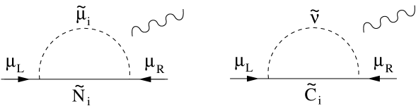
Figure 1: Supersymmetric diagrams contributing to $a_{\mu}$ at one-loop.

First, the magnetic moment operator is a helicity-flipping interaction. Thus any diagram which contributes to $a_{\mu}$ must involve a helicity flip somewhere along the fermion current. This automatically divides the diagrams into two classes: those with helicity flips on the external legs and those with flips on an internal line. For those in the first class, the amplitude must scale as $m_{\mu}$; for those in the second, the amplitudes can scale instead by $m_{\rm SUSY}$, where $m_{\rm SUSY}$ represents the mass of the internal SUSY fermion (a chargino or neutralino). Since $m_{\rm SUSY}\gg m_{\mu}$, it is the latter class that will typically dominate the SUSY contribution to $a_{\mu}$. Therefore we will restrict further discussion to this latter class of diagrams alone.

Secondly, the interaction of the neutralinos and charginos with the (s)muons and sneutrinos occurs either through their higgsino or gaugino components. Thus each vertex implies a factor of either $y_{\mu}$ (the muon Yukawa coupling) or $g$ (the weak and/or hypercharge gauge coupling). Given two vertices, the diagrams therefore scale as $y_{\mu}^{2}$, $gy_{\mu}$ or $g^{2}$. In the Standard Model, $y_{\mu}$ is smaller than $g$ by roughly $10^{-3}$. In the minimal SUSY standard model (MSSM) at low $\tan\beta$, this ratio is essentially unchanged, but because $y_{\mu}$ scales as $1/\cos\beta$, at large $\tan\beta$ ($\sim 60$) the ratio can be reduced to roughly $10^{-1}$. Thus we can safely drop the $y_{\mu}^{2}$ contributions from our discussions, but at large $\tan\beta$ we must preserve the $gy_{\mu}$ pieces as well as the $g^{2}$ pieces.

The pieces that we will keep are therefore shown in Figures 2. In Fig. 2(a)-(e) are shown the five neutralino contributions which scale as $g^{2}$ or $gy_{\mu}$; in Fig. 2(f) is the only chargino contribution, scaling as $gy_{\mu}$. The contributions to $a_{\mu}$ from the $i$th neutralino and the $m$th smuon due to each of these component diagrams are found to be:

$$\delta a_{\mu}=\frac{1}{48\pi^{2}}\frac{m_{\mu}m_{{\tilde{N}}_{i}}}{m_{{\tilde{\mu}}_{m}}^{2}}F_{2}^{N}(x_{im})\times\left\{\begin{array}[]{lc}g_{1}^{2}N_{i1}^{2}X_{m1}X_{m2}&({\tilde{B}}{\tilde{B}})\\ g_{1}g_{2}N_{i1}N_{i2}X_{m1}X_{m2}&({\tilde{W}}{\tilde{B}})\\ -\sqrt{2}g_{1}y_{\mu}N_{i1}N_{i3}X_{m2}^{2}&({\tilde{H}}{\tilde{B}})\\ \frac{1}{\sqrt{2}}g_{1}y_{\mu}N_{i1}N_{i3}X_{m1}^{2}&({\tilde{B}}{\tilde{H}})\\ \frac{1}{\sqrt{2}}g_{2}y_{\mu}N_{i2}N_{i3}X_{m1}^{2}&({\tilde{W}}{\tilde{H}})\end{array}\right.$$ (9)

and for the $k$th chargino and the sneutrino:

$$\delta a_{\mu}=-\frac{1}{24\pi^{2}}\frac{m_{\mu}m_{{\tilde{C}}_{k}}}{m_{{\tilde{\nu}}}^{2}}F_{2}^{C}(x_{k})\,g_{2}y_{\mu}U_{k2}V_{k1}.\quad\quad({\tilde{W}}{\tilde{H}})$$ (10)

The matrices $N$, $U$ and $V$ are defined in the appendix along with the functions $F_{2}^{N,C}$. A careful comparison to the equations in the appendix will reveal that we have dropped a number of complex conjugations in the above expressions; it has been shown previously [3, 4] that the SUSY contributions to $a_{\mu}$ are maximized for real entries in the mass matrices and so we will not retain phases in our discussion.

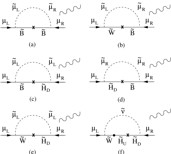
Figure 2: Diagrams contributing to $a_{\mu}$ in the interaction eigenbasis.

In many of the previous analyses of the MSSM parameter space, it was found that it is the chargino-sneutrino diagram at large $\tan\beta$ that can most easily generate values of $\delta a_{\mu}$ large enough to explain the observed discrepancy. From this observation, one can obtain an upper mass bound on the lightest chargino and the muon sneutrino. However, this behavior is not completely generic. For example, Martin and Wells emphasized that the ${\tilde{B}}{\tilde{B}}$ neutralino contribution could by itself be large enough to generate the old observed excess in $a_{\mu}$, and since it has no intrinsic $\tan\beta$ dependence, they could explain the old excess with $\tan\beta$ as low as 3. We can reproduce their result in a simple way because the ${\tilde{B}}{\tilde{B}}$ contribution has a calculable upper bound at which the smuons mix at $45^{\circ}$, $m_{{\tilde{\mu}}_{1}}\ll m_{{\tilde{\mu}}_{2}}$, and $m_{{\tilde{N}}_{1}}\ll m_{{\tilde{N}}_{2,3,4}}$ with ${\tilde{N}}_{1}={\tilde{B}}$. Then

$$\left|\delta a_{\mu}\right|_{({\tilde{B}}{\tilde{B}})}\leq\frac{g_{1}^{2}}{32\pi^{2}}\frac{m_{\mu}m_{{\tilde{N}}_{1}}}{m_{{\tilde{\mu}}_{1}}^{2}}\simeq 3800\times 10^{-10}\times\left(\frac{m_{{\tilde{N}}_{1}}}{100\,{\rm GeV}}\right)\left(\frac{100\,{\rm GeV}}{m_{{\tilde{\mu}}_{1}}}\right)^{2}$$ (11)

where we have used the fact that $(X_{11}X_{12})\leq\frac{1}{2}$ and $F_{2}^{N}\leq 3$ and have included a 7% two-loop suppression factor. Though any real model will clearly suppress this contribution somewhat, this is still $10^{2}$ times larger than needed experimentally.

This pure ${\tilde{B}}{\tilde{B}}$ scenario is actually an experimental worst-case, particularly for hadron colliders. The only sparticles that are required to be light are a single neutralino (which is probably ${\tilde{B}}$-like) and a single ${\tilde{\mu}}$. The neutralino is difficult to produce, and if stable, impossible to detect directly. The neutralino could be indirectly observed in the decay of the ${\tilde{\mu}}$ as missing energy, but production of a ${\tilde{\mu}}$ at a hadron machine is highly suppressed. In the worst of all possible worlds, E821 could be explained by only these two light sparticles, with the rest of the SUSY spectrum hiding above a TeV. Further, even the “light” sparticles can be too heavy to produce at a $500\,{\rm GeV}$ linear collider. While this case is in no way generic, it demonstrates that the E821 excess does not provide any sort of no-lose theorem (even at $1\sigma$) for the Tevatron, the LHC or the NLC.

This raises an important experimental question: how many of the MSSM states must be “light” in order to explain the E821 data? In the worst-case, it would appear to be only two. Even in the more optimistic scenario in which the chargino diagram dominates $\delta a_{\mu}$, the answer naively appears to be two: a single chargino and a single sneutrino. In this limit,

$$\left|\delta a_{\mu}\right|_{({\tilde{C}}{\tilde{\nu}})}\leq\frac{g_{2}y_{\mu}}{24\pi^{2}}\frac{m_{\mu}m_{{\tilde{C}}_{1}}}{m_{\tilde{\nu}}^{2}}\left|F^{C}_{2}\right|_{\rm max}\lower 3.01385pt\hbox{$\;\stackrel{{\scriptstyle\textstyle<}}{{\sim}}\;$}2600\times 10^{-10}\times\left(\frac{m_{{\tilde{C}}_{1}}}{100\,{\rm GeV}}\right)\left(\frac{100\,{\rm GeV}}{m_{{\tilde{\nu}}}}\right)^{2}\left(\frac{\tan\beta}{30}\right)$$ (12)

where we have bounded $|F_{2}^{C}|$ by 10 by assuming $m_{\tilde{\nu}}\lower 3.01385pt\hbox{$\;\stackrel{{\scriptstyle\textstyle<}}{{\sim}}\;$}1\,{\rm TeV}$. But this discussion is overly simplistic, as we will see.

1.2 Mass correlations

There are a total of 9 separate sparticles which can enter the loops in Fig. 1: 1 sneutrino, 2 smuons, 2 charginos and 4 neutralinos. The mass spectrum of these 9 sparticles is determined entirely by 7 parameters in the MSSM: 2 soft slepton masses($m_{L}$, $m_{R}$), 2 gaugino masses ($M_{1}$, $M_{2}$), the $\mu$-term, a soft trilinear slepton coupling ($A_{\tilde{\mu}}$) and finally $\tan\beta$. Of these, $A_{\tilde{\mu}}$ plays almost no role at all and so we leave it out of our discussions (see the appendix). And in some well-motivated SUSY-breaking scenarios, $M_{1}$ and $M_{2}$ are also correlated. Thus there are either 5 or 6 parameters responsible for setting 9 sparticle masses. There are clearly non-trivial correlations among the masses which can be exploited in setting mass limits on the sparticles.

First, there are well-known correlations between the chargino and neutralino masses; for example, a light charged ${\tilde{C}}_{i}\sim{\tilde{W}}$ implies a light neutral ${\tilde{N}}_{j}\sim{\tilde{W}}$ and vice-versa.

There are also correlations in mixed systems (i.e., the neutralinos, charginos and smuons) between the masses of the eigenstates and the size of their mixings. Consider the case of the smuons in particular; their mass matrix is given in the appendix. On diagonalizing, the left-right smuon mixing angle is given simply by:

$$\tan 2\theta_{\tilde{\mu}}\simeq\frac{2m_{\mu}\mu\tan\beta}{M_{L}^{2}-M_{R}^{2}}.$$ (13)

The chargino contribution is maximized for large smuon mixing and large mixing occurs when the numerator is of order or greater than the denominator; since the former is suppressed by $m_{\mu}$, one must compensate by having either a very large $\mu$-term in the numerator or nearly equal $M_{L}$ and $M_{R}$ in the denominator, both of which have profound impacts on the spectrum.

There is one more correlation/constraint that we feel is natural to impose on the MSSM spectrum: slepton mass universality. It is well-known that the most general version of the MSSM produces huge flavor-changing neutral currents (FCNCs) unless some external order is placed on the MSSM spectrum. By far, the simplest such order is for sparticles with the same gauge quantum numbers to be degenerate. This requirement is most stringent in the squark sector, but also holds in the slepton sector due to non-observation of $\mu\to e\gamma$ and $\tau\to\mu\gamma$. In any case, mechanisms which generate degeneracy in the squarks usually do so among the sleptons as well. Thus we assume $m_{{\tilde{\tau}}_{L}}=m_{{\tilde{\mu}}_{L}}\equiv m_{L}$ and $m_{{\tilde{\tau}}_{R}}=m_{{\tilde{\mu}}_{R}}\equiv m_{R}$. Then the mass matrix for the stau sector is identical to that of the smuons with the replacement $m_{\mu}\to m_{\tau}$ in the off-diagonal elements. This enhancement of the mixing in the stau sector by $m_{\tau}/m_{\mu}\simeq 17$ implies that $m_{{\tilde{\tau}}_{1}}<m_{{\tilde{\mu}}_{1}}$. In particular, if

$$M_{L}^{2}M_{R}^{2}<m^{2}_{\tau}\,\mu^{2}\tan^{2}\beta$$ (14)

then $m^{2}_{{\tilde{\tau}}_{1}}<0$ and QED will be broken by a stau vev. Given slepton universality, this imposes a constraint on the smuon mass matrix:

$$M_{L}^{2}M_{R}^{2}>\left(\frac{m_{\tau}}{m_{\mu}}\right)^{2}m_{\mu}^{2}\,\mu^{2}\tan^{2}\beta$$ (15)

or on the smuon mixing angle:

$$\tan 2\theta_{\tilde{\mu}}<\left(\frac{m_{\mu}}{m_{\tau}}\right)\frac{2M_{L}M_{R}}{M_{L}^{2}-M_{R}^{2}}$$ (16)

where $M_{L,R}$ are the positive roots of $M^{2}_{L,R}$. While not eliminating the possibility of $\theta_{\tilde{\mu}}\simeq 45^{\circ}$, this formula shows that a fine-tuning of at least 1 part in 17 is needed to obtain ${\cal O}(1)$ mixing. We will not apply any kind of fine-tuning criterion to our analysis, yet we will find that this slepton mass universality constraint sharply reduces the upper bounds on slepton masses which we are able to find in our study of points in MSSM parameter space.

(As an aside, if one assumes slepton mass universality at some SUSY-breaking messenger scale above the weak scale, Yukawa-induced corrections will break universality by driving the stau masses down. This effect would further tighten our bounds on smuon masses and mixings.)

The above discussion has an especially large impact on the worst-case scenario in which the ${\tilde{B}}{\tilde{B}}$ contributions dominates $\delta a_{\mu}$. For generic points in MSSM parameter space, one expects that $\tan 2\theta_{\tilde{\mu}}\lower 3.01385pt\hbox{$\;\stackrel{{\scriptstyle\textstyle<}}{{\sim}}\;$}1/17$ which reduces the size of the ${\tilde{B}}{\tilde{B}}$ contribution by a factor of 17. As a byproduct, the masses required for explaining the E821 anomaly are pushed back toward the experimentally accessible region.

2 Numerical results

Now that we have established the basic principle of our analysis, we will carry it out in detail. We will concentrate on three basic cases. The first case is the one most often considered in the literature: gaugino mass unification. Here one assumes that the weak-scale gaugino mass parameters ($M_{1}$ and $M_{2}$) are equal at the same scale at which the gauge couplings unify. This implies that at the weak scale $M_{1}=(5/3)(\alpha_{1}/\alpha_{2})M_{2}$. The second case we consider is identical to the first with the added requirement that the lightest SUSY sparticle (LSP) be a neutralino. This requirement is motivated by the desire to explain astrophysical dark matter by a stable LSP. Finally we will also consider the most general case in which all relevant SUSY parameters are left free independent of each other; we will refer to this as the “general MSSM” case.

The basic methodology is simple: we put down a logarithmic grid on the space of MSSM parameters ($M_{1}$, $M_{2}$, $m_{L}$, $m_{R}$ and $\mu$) for several choices of $\tan\beta$. The grid extends from $10\,{\rm GeV}$ for $M_{1}$, $M_{2}$ and $\mu$, and from $50\,{\rm GeV}$ for $m_{L,R}$, up to $2\,{\rm TeV}$ for all mass parameters. For the case in which gaugino unification is imposed $M_{2}$ is no longer a free parameter and our grid contains $10^{8}$ points. For the general MSSM case our grid contains $3\times 10^{9}$ points. Only $\mu>0$ is considered since that maximizes the value of $\delta a_{\mu}$. Finally, for our limits on $\tan\beta$ we used an adaptive mesh routine which did a better job of maximizing $\delta a_{\mu}$ over the space of MSSM inputs. By running with grids of varying resolutions and offsets we estimate the error on our mass bounds to be less than $\pm 5\%$.

2.1 Bounds on the lightest sparticles

Perhaps the most important information that can be garnered from the E821 data is an upper bound on the scale of sparticle masses. In particular, one can place upper bounds on the masses of the lightest sparticle(s) as a function of $\delta a_{\mu}$. Here we will derive bounds on the lightest slepton and chargino, but we will also derive bounds on the lightest several sparticles, independent of their identity.

These bounds on additional light sparticles provide an important lesson. Without them there remains the very real possibility that the E821 data is explained by a pair of light sparticles and that the remaining SUSY spectrum is out of reach experimentally. But our additional bounds will give us some indication not only of where we can find SUSY, but also of how much information we might be able to extract about the fundamental parameters of SUSY — the more sparticles we detect and measure, the more information we will have for disentangling the soft-breaking sector of the MSSM.

In Fig. 3 we have shown the upper mass bounds for the lightest four sparticles assuming gaugino mass unification. These bounds are not bounds on individual species of sparticles (which will come in the next section and always be larger than these bounds) but simply bounds on whatever sparticle happens to be lightest. The important points to note are: (i) the maximum values of the mass correspond to the largest value of $\tan\beta$, which is to be expected given dominance of the chargino diagram at large $\tan\beta$; (ii) the $1\sigma$ limit without (with) the $\tau$ data requires at least 2 sparticles to lie below roughly $490\,(990)\,{\rm GeV}$; (iii) for the central value of the E821 data, at least 4 sparticles must lie below $585\,(915)\,{\rm GeV}$; and (iv) for low values of $\tan\beta$ a maximum value of $\delta a_{\mu}$ is reached (we will return to this later).

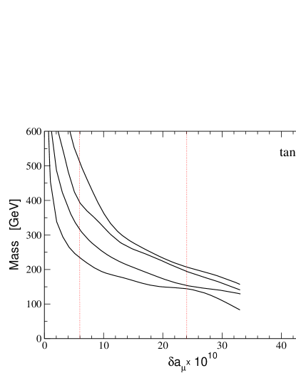
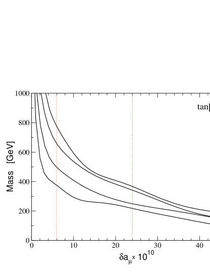
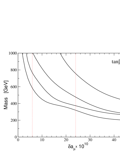
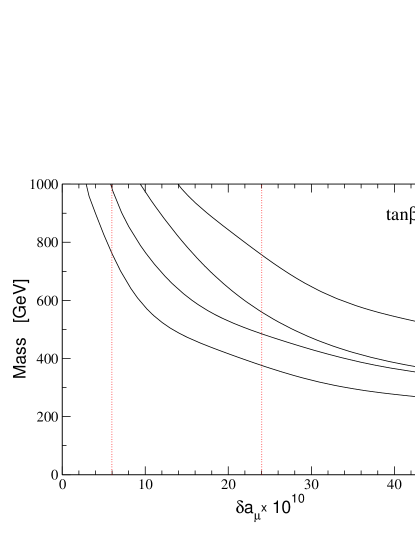
Figure 3: Bounds on the masses of the four lightest sparticles as a function of $\delta a_{\mu}$ for $\tan\beta=3$, 10, 30 and 50. These figures assume gaugino unification only. The vertical dotted lines represent the $1\sigma$ bounds using the $\tau$-decay data ($\delta a_{\mu}=6$) or not ($\delta a_{\mu}=24$).

The same plots could be produced with the additional assumption that the LSP be a neutralino, but we will only show the case for the LSP bound, in Fig. 4. In this figure, the solid lines correspond to a neutralino LSP, while the dotted lines are for the more general case discussed above (i.e., they match the lines in the $\tan\beta=50$ plot of Fig. 3). Notice that for $\delta a_{\mu}\lower 3.01385pt\hbox{$\;\stackrel{{\scriptstyle\textstyle>}}{{\sim}}\;$}40\times 10^{-10}$ there is little difference between the cases with and without a neutralino LSP. At the extreme upper and lower values of $\tan\beta$ there is also little difference. It is only for the intermediate values of $\tan\beta$ that the mass bound shifts appreciably; for $\tan\beta=10$ it comes down by as much as $50\,{\rm GeV}$ when one imposes a neutralino LSP.

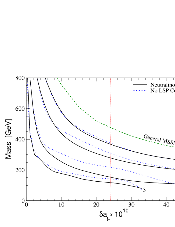
Figure 4: Bound on the mass of the LSP as a function of $\delta a_{\mu}$ for $\tan\beta=3$, 5, 10, 30 and 50. The dotted lines assume gaugino unification only while the solid lines require additionally that the LSP is a neutralino. The dashed line is the bound in the general MSSM, calculated at $\tan\beta=50$.

Finally, we consider the most general MSSM case, i.e., without gaugino unification. Here the correlations are much less pronounced, but interesting bounds still exist. For example the central value of the E821 data still demands at least 3 sparticles below $525\,(770)\,{\rm GeV}$. In figure 5 we demonstrate this explicitly by plotting the masses of the four lightest sparticles for $\tan\beta=50$ and a wide range of $\delta a_{\mu}$. (We also plot the mass bound on the LSP in Fig. 4 with the label “General MSSM.”) We see that dropping the gaugino unification requirement has one primary effect: the mass of the LSP is significantly increased. This is because the LSP in the unified case is usually a ${\tilde{N}}_{1}\sim{\tilde{B}}$ but isn’t itself responsible for generating $\delta a_{\mu}$. In the general case, the LSP must participate in $\delta a_{\mu}$ (otherwise its mass could be arbitrarily large) and so is roughly the mass of the second lightest sparticle in the unified case, whether that be a ${\tilde{\mu}}$ or ${\tilde{C}}$. Otherwise the differences between the more general MSSM and the gaugino unified MSSM are small.

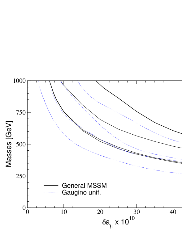
Figure 5: Bounds on the masses of the four lightest sparticles as a function of $\delta a_{\mu}$ for $\tan\beta=50$. The dotted lines assume gaugino unification only while the solid lines are for the general MSSM.

We have summarized all this data on the LSP in Table 1 where we have shown the mass bounds using the $1\sigma$ limit of the E821 data on the LSP for various $\tan\beta$ values with our various assumptions. The numbers represent the bounds without (with) the inclusion of the $\tau$ decay data. The last line in the table represents an upper bound for any model with $\tan\beta\leq 50$: $m_{\rm LSP}<475\,{\rm GeV}\,(1\,{\rm TeV})$ for the E821 $1\sigma$ lower bounds of $\delta a_{\mu}$. But perhaps of equal importance are the bounds on the next 2 lightest sparticles (the “2LSP” and “3LSP”): Using $a_{\mu}$ calculated without $\tau$-decay data, $m_{\rm 2LSP}<485\,{\rm GeV}$ and $m_{\rm 3LSP}<630\,{\rm GeV}$; for the value of $a_{\mu}$ calculated with the $\tau$ data, $m_{\rm 2LSP}<1\,{\rm TeV}$, while $m_{\rm 3LSP}$ is pushed somewhat above $1\,{\rm TeV}$. Note that the bound on the 2LSP is essentially identical to that on the LSP. The central value of the E821 anomaly further implies a fourth (third) sparticle below $1\,{\rm TeV}$ even in this most general case.

Mass	General	Gaugino	+ Dark
Bound	MSSM	Unification	Matter
$\tan\beta=3$	205 (331)	140 (230)	115 (215)
5	235 (395)	170 (280)	135 (280)
10	280 (475)	215 (350)	150 (325)
30	340 (750)	305 (580)	275 (565)
50	475 (1000)	370 (765)	365 (765)

Table 1: Upper bounds on the mass (in GeV) of the lightest sparticle for the general MSSM, the MSSM with gaugino mass unification, and the MSSM with gaugino mass unification plus a neutralino LSP. The entries represent the $1\sigma$ bound without (with) the inclusion of the $\tau$ decay data. The boldfaced $\tan\beta=50$ entries represent upper bounds over all $\tan\beta\leq 50$.

2.2 Bounds on the sparticle species

In the previous subsection, we derived bounds on the lightest sparticles, independent of the identity of those sparticles. Another important piece of information that can be provided by this analysis is bounds on individual species of sparticles, for example, on the charginos or on the smuons. These bounds will of necessity be higher than those derived in the previous section, but still provide important information about how and where to look for SUSY. In particular, they can help us gauge the likelihood of finding SUSY at Run II of the Tevatron or at the LHC.

There is one complication in obtaining these bounds. At low $\tan\beta$ the data is most easily explained by the neutralino diagrams and as such there must be at least one light smuon and one light neutralino. At larger $\tan\beta$ contributions from the chargino diagrams dominate, implying a light chargino and sneutrino. However the correlations already discussed preserve the bounds on the various species over the whole range of $\tan\beta$. A bound on $m_{\tilde{\nu}}$ implies a bound on $m_{{\tilde{\mu}}_{1}}$, and a bound on $m_{{\tilde{C}}_{1}}$ implies a bound on at least one of the $m_{{\tilde{N}}_{i}}$, and in certain cases (such as gaugino unification), the converses may be true as well.

We have shown in Fig. 6 the mass bounds on ${\tilde{\mu}}_{1}$ and ${\tilde{N}}_{1}$ under the assumption of gaugino unification; a plot for ${\tilde{C}}_{1}$/${\tilde{N}}_{2}$ will appear later in our discussion of Tevatron physics. Note that ${\tilde{N}}_{1}$ must lie below $500\,(950)\,{\rm GeV}$, even for large $\tan\beta$, thanks to the gaugino unification condition, while ${\tilde{\mu}}_{1}$ can be heavier but must still lie below $915\,(1800)\,{\rm GeV}$ at $1\sigma$.

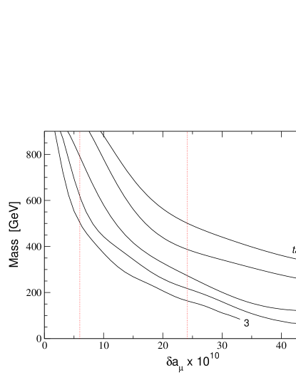
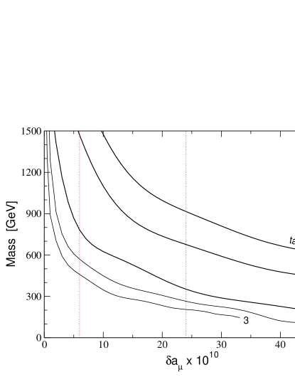
Figure 6: Bounds on the masses of ${\tilde{N}}_{1}$ and ${\tilde{\mu}}_{1}$ as a function of $\delta a_{\mu}$ for various $\tan\beta$ with gaugino mass unification assumed. Again, the vertical dotted lines indicate $1\sigma$ bounds without (with) the inclusion of the $\tau$ decay data.

Finally, we can consider the general MSSM without gaugino unification. The results are shown schematically in Fig. 7 where the general MSSM bounds (solid lines) are shown alongside the gaugino unification bounds (dashed lines).

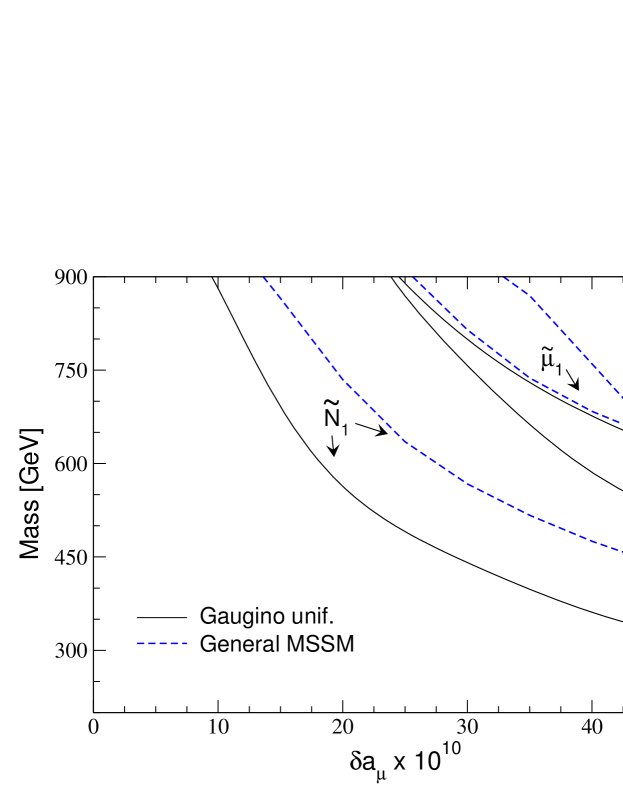
Figure 7: Bounds on the masses of ${\tilde{\mu}}_{1}$, ${\tilde{C}}_{1}$, and ${\tilde{N}}_{1}$ as a function of $\delta a_{\mu}$ for $\tan\beta=50$, with gaugino unification (solid) and in the general MSSM (dashed). The two lines for the ${\tilde{\mu}}_{1}$ essentially overlap.

We can see from the figure that the bound on the ${\tilde{\mu}}_{1}$ is essentially identical to that in the gaugino unification picture. However the gaugino masses have shifted, and the reason is no mystery. Once again, the lightest neutralino is no longer a ${\tilde{B}}$-like spectator to the magnetic moment, but is a ${\tilde{W}}$-like partner of a participating ${\tilde{W}}$-like chargino.

The results of these plots for the current discrepancy are summarized as follows. For the MSSM with gaugino unification, the lightest neutralino must fall below $500\,(950)\,{\rm GeV}$ for a $1\sigma$ deviation. The lighter smuon must lie below $915\,{\rm GeV}$ ($1.8\,{\rm TeV}$). Without the $\tau$-decay data, the lighter chargino falls below $890\,{\rm GeV}$; using the $\tau$ data, the bound rises above $2\,{\rm TeV}$.

For the worst case, the general MSSM, the smuon bound increases by only about $50\,{\rm GeV}$ over the gaugino unification limits and the neutralino bounds increase to $890\,{\rm GeV}$ (over $1\,{\rm TeV}$), only slightly higher than the unified case. However, the bounds on the lighter chargino jump above $2\,{\rm TeV}$.

2.3 Bounds on $\tan\beta$

The final bound we will investigate using the E821 data is on $\tan\beta$. There had been, after the appearance of the original E821 data, some discussion in the literature about which values of $\tan\beta$ were capable of explaining it. In particular, at lower $\tan\beta$ there is a real suppression in the maximum size of $\delta a_{\mu}$. In Figure 8 we have shown the maximum attainable value of $\delta a_{\mu}$ as a function of $\tan\beta$ in the general MSSM; adding the assumption of gaugino unification changes the figure only slightly.

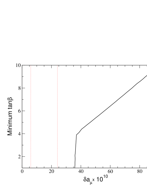
Figure 8: Bounds on $\tan\beta$ as a function of $\delta a_{\mu}$ for the general MSSM. The dotted lines represent the $1\sigma$ limits, without (with) the inclusion of the $\tau$ decay data.

The limit in Fig. 8 clearly divides into two regions. At $\delta a_{\mu}>36\times 10^{-10}$ the chargino contribution dominates and thus $\delta a_{\mu}\propto y_{\mu}$, scaling linearly with $\tan\beta$. At lower $\delta a_{\mu}$, however, both neutralino and chargino contributions can be important so it becomes possible to generate $\delta a_{\mu}$ with much smaller values of $\tan\beta$ than would be possible from the charginos alone. The E821 data does not therefore imply any bound on $\tan\beta$ whatsoever, neither at $1\sigma$ nor at the experimental central value. Further reductions in the size of the error bars will not change this result, so long as the central value remains at or below its current $1\sigma$ upper bound.

2.4 Implications for the Tevatron

At its simplest level, the measurement of $\delta a_{\mu}$, an anomaly in the lepton sector, has little impact on the Tevatron, a hadron machine. In particular, the light smuons associated with $\delta a_{\mu}$ cannot be directly produced at the Tevatron, occurring only if heavier non-leptonic states are produced which then decay to sleptons. In the calculation of $a_{\mu}$, the only such sparticles are the neutralinos and charginos. These states can be copiously produced and in fact form the initial state for the “gold-plated” SUSY trilepton signature.

Of particular interest for the trilepton signature are the masses of the lighter chargino (${\tilde{C}}_{1}$) and 2nd lightest neutralino (${\tilde{N}}_{2}$). Studies of mSUGRA parameter space indicate that the sensitivity to the trilepton signature at Run II/III of the Tevatron depends strongly on the mass of sleptons which can appear in the gaugino decay chains. For heavy sleptons, the Tevatron is only sensitive to gaugino masses in the range [20] $m_{{\tilde{C}}_{1},{\tilde{N}}_{2}}\lower 3.01385pt\hbox{$\;\stackrel{{\scriptstyle\textstyle<}}{{\sim}}\;$}130$ to $140\,{\rm GeV}$ for $10\,\mbox{fb}^{-1}$ of luminosity and $145$ to $155\,{\rm GeV}$ for $30\,\mbox{fb}^{-1}$, where the quoted ranges take one from low to high $\tan\beta$. However, for light sleptons (below about $200\,{\rm GeV}$) the range is considerably extended, up to gaugino masses around 190 to $210\,{\rm GeV}$.

It is impossible in the kind of analysis presented here to comment on the expected cross-sections for the neutralino-chargino production (for example, there is no information in $a_{\mu}$ on the masses of the $t$-channel squarks) but we can examine the mass bounds on ${\tilde{C}}_{1}$ and ${\tilde{N}}_{2}$. In Fig. 9 we have shown just that: the upper bound on the heavier of either ${\tilde{C}}_{1}$ or ${\tilde{N}}_{2}$ as a function of $\delta a_{\mu}$ for several values of $\tan\beta$.

A few comments are in order on the figure. First, this figure assumes gaugino unification; dropping that assumption can lead to significantly heavier and unequal masses for the ${\tilde{N}}_{2}$ and ${\tilde{C}}_{1}$. Second, we have also assumed a neutralino LSP; this is to be expected since the event topology for the trilepton signal assumes a stable, neutralino LSP. Finally, on the $y$-axis is actually plotted $m_{{\tilde{C}}_{1}}$, but in every case we examined with gaugino unification, the difference in the maximum masses of ${\tilde{C}}_{1}$ and ${\tilde{N}}_{2}$ differed by at most a few GeV. This is because they are both dominantly wino-like in the unified case and thus have masses $\simeq M_{2}$.

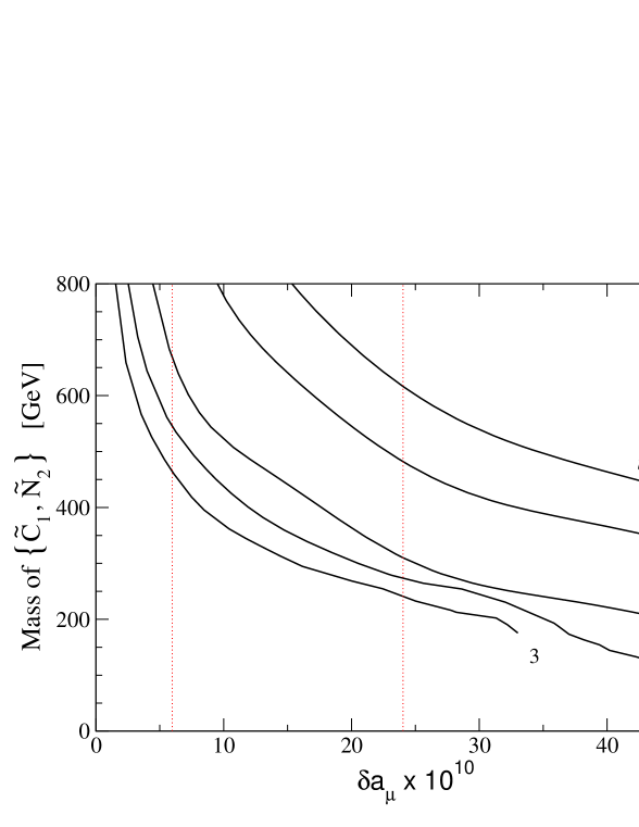
Figure 9: Mass bounds on ${\tilde{C}}_{1}$ and ${\tilde{N}}_{2}$ (where $m_{{\tilde{C}}_{1}}\simeq m_{{\tilde{N}}_{2}}$) as a function of $\delta a_{\mu}$ for $\tan\beta=3$, 5, 10, 30 and 50. The dotted lines represent the $1\sigma$ bounds without (with) the inclusion of the $\tau$ decay data. This figure assumes gaugino unification and a neutralino LSP.

From the figure it is clear that one cannot devise a no-lose theorem for the Tevatron from current E821 data. However, if $\tan\beta$ is small and $\delta a_{\mu}\geq 35\times 10^{-10}$ (the current central value using only $e^{+}e^{-}$ data) then the gauginos may be within the Tevatron’s reach. We must also emphasize that these are upper bounds on the sparticle masses and in no way represent best fits or preferred values. Thus, for small $\tan\beta$, there is reason to hope that the Tevatron will be able to probe the gaugino sector in Run II or III; for larger $\tan\beta$ there is little information about SUSY at the Tevatron to be garnered from $a_{\mu}$.

2.5 Implications for a Linear Collider

A consensus has emerged in favor of building a $\sqrt{s}=500\,{\rm GeV}$ linear collider, presumably a factory for sparticles with masses below $250\,{\rm GeV}$. What does the measurement of $a_{\mu}$ tell us with regards to our chances for seeing SUSY at $\sqrt{s}=500\,{\rm GeV}$? And how many sparticles will be actually accessible to such a collider?

The analysis of the previous section can put a lower bound on the number of observable sparticles at a linear collider as a function of $\delta a_{\mu}$ and $\tan\beta$ and we show those numbers as a histogram in Fig. 10. In this figure, we have shown the minimum number of sparticles with mass below $250\,{\rm GeV}$ for $\tan\beta=3$, 10, 30 and 50, assuming gaugino unification. In the graph, the thinner bars represent smaller $\tan\beta$. As is to be expected, the number of light states increases with increasing $\delta a_{\mu}$ and with decreasing $\tan\beta$. However note that there are no $\tan\beta=3$ lines for $\delta a_{\mu}\geq 40\times 10^{-10}$ since there is no way to explain such large $\delta a_{\mu}$ values at low $\tan\beta$.

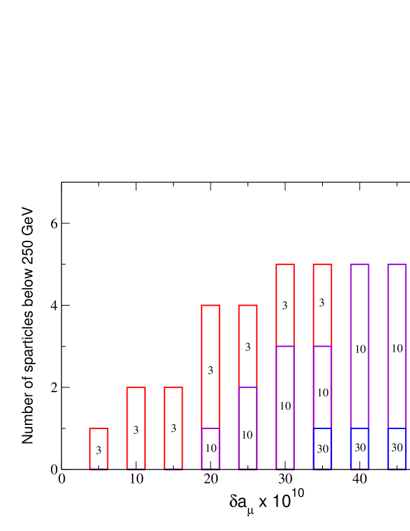
Figure 10: Minimum number of sparticles directly observable at a $\sqrt{s}=500\,{\rm GeV}$ linear collider as a function of $\delta a_{\mu}$. The bars represent $\tan\beta=3$, 10, 30 and 50. This graph assumes gaugino unification but does not include additional sleptons implied by slepton mass universality.

We see from the figure that at low $\tan\beta$, there is a $1\sigma$ “guarantee” that at least 1 to 4 sparticles will be produced at a $500\,{\rm GeV}$ linear collider, depending on whether the $\tau$-decay is used. This counting does not include extra sleptons due to slepton mass universality; for example, a light muon sneutrino also implies light tau and electron sneutrinos, and likewise for the charged smuon. We see also that for $\tan\beta\lower 3.01385pt\hbox{$\;\stackrel{{\scriptstyle\textstyle>}}{{\sim}}\;$}30$ there is no such guarantee that a $500\,{\rm GeV}$ machine would produce on-shell sparticles; this is not to be taken to mean that one should not expect their production, simply that $a_{\mu}$ cannot guarantee it.

A similar bar graph can also be made for a $1\,{\rm TeV}$ machine, though we do not show it here. However the relevant numbers can be inferred from Fig. 3.

Note that any particular class of models, such as gravity- or gauge-mediated SUSY-breaking, may not saturate the bounds presented here. That is, other constraints may rule out all regions of parameter space in which $\delta a_{\mu}$ exceeds some maximum value. However if a model does allow a particular value of $\delta a_{\mu}$, then pursuant to the conditions discussed here, that model must have at least as many light particles as the number given above.

3 Conclusions

Deviations in the muon anomalous magnetic moment have long been advertised as a key hunting ground for indirect signatures of SUSY. However, the current experimental excess is too small, given the large theoretical uncertainties, to provide statistically significant evidence for SUSY.

The most recent Standard Model calculations indicate an excess of either $1.5\sigma$ or $3.2\sigma$. If one were to accept the E821 anomaly as evidence for SUSY (at either of these values), then a number of statements can be inferred at the $1\sigma$ confidence level:

• The lightest sparticle must lie below $475\,{\rm GeV}\,(1\,{\rm TeV})$;

• For models with unified gaugino masses, there must be at least 2 sparticles with masses below $585\,{\rm GeV}\,(1\,{\rm TeV})$;

• There is no lower bound on $\tan\beta$.

Bounds on individual species of sparticles are weaker, usually falling at or above $1\,{\rm TeV}$.

However, these pessimistic bounds are over all $\tan\beta$, which means effectively that they are the bounds when $\tan\beta=50$, the maximum value we considered. For low $\tan\beta$, the bounds on sparticle masses are much smaller. At $\tan\beta=3$ and with gaugino unification and a neutralino LSP, there must be a sparticle below $115\,(215)\,{\rm GeV}$, within the range accessible in the very near future. So, while the bounds placed on SUSY by $a_{\mu}$ are relatively weak when no constraints are placed on the MSSM, constraining the model by demanding gaugino unification or low(er) $\tan\beta$ can bring down the mass bounds into the experimentally interesting region.

Appendix

The supersymmetric contributions to $a_{\mu}$ are generated by diagrams involving charged smuons with neutralinos, and sneutrinos with charginos. The most general form of the calculation, including phases, takes the form (we follow Ref. [4]):

$$\delta a_{\mu}^{({\tilde{N}})} = \frac{m_{\mu}}{16\pi^{2}}\sum_{i,m}\left\{-\frac{m_{\mu}}{12m^{2}_{{\tilde{\mu}}_{m}}}(|n^{L}_{im}|^{2}+|n^{R}_{im}|^{2})F^{N}_{1}(x_{im})+\frac{m_{{\tilde{N}}_{i}}}{3m^{2}_{{\tilde{\mu}}_{m}}}{\rm Re}[n^{L}_{im}n^{R}_{im}]F^{N}_{2}(x_{im})\right\}$$

$$\delta a_{\mu}^{({\tilde{C}})} = \frac{m_{\mu}}{16\pi^{2}}\sum_{k}\left\{\frac{m_{\mu}}{12m^{2}_{{\tilde{\nu}}}}(|c^{L}_{k}|^{2}+|c^{R}_{k}|^{2})F^{C}_{1}(x_{k})+\frac{2m_{{\tilde{C}}_{k}}}{3m^{2}_{{\tilde{\nu}}}}{\rm Re}[c^{L}_{k}c^{R}_{k}]F^{C}_{2}(x_{k})\right\}$$ (17)

where $i=1,2,3,4$, $m=1,2$, and $k=1,2$ label the neutralino, smuon and chargino mass eigenstates respectively, and

$$n^{R}_{im} = \sqrt{2}g_{1}N_{i1}X_{m2}+y_{\mu}N_{i3}X_{m1},$$

$$n^{L}_{im} = {1\over\sqrt{2}}\left(g_{2}N_{i2}+g_{1}N_{i1}\right)X_{m1}^{*}-y_{\mu}N_{i3}X^{*}_{m2},$$

$$c^{R}_{k} = y_{\mu}U_{k2},$$

$$c^{L}_{k} = -g_{2}V_{k1},$$ (18)

$y_{\mu}=g_{2}m_{\mu}/\sqrt{2}m_{W}\cos\beta$ is the muon Yukawa coupling, and $g_{1,2}$ are the U(1) hypercharge and SU(2) gauge couplings. The loop functions depend on the variables $x_{im}=m^{2}_{{\tilde{N}}_{i}}/m^{2}_{{\tilde{\mu}}_{m}}$, $x_{k}=m^{2}_{{\tilde{C}}_{k}}/m^{2}_{{\tilde{\nu}}}$ and are given by

$$F^{N}_{1}(x) = \frac{2}{(1-x)^{4}}\left[1-6x+3x^{2}+2x^{3}-6x^{2}\ln x\right]$$

$$F^{N}_{2}(x) = \frac{3}{(1-x)^{3}}\left[1-x^{2}+2x\ln x\right]$$

$$F^{C}_{1}(x) = \frac{2}{(1-x)^{4}}\left[2+3x-6x^{2}+x^{3}+6x\ln x\right]$$

$$F^{C}_{2}(x) = -\frac{3}{2(1-x)^{3}}\left[3-4x+x^{2}+2\ln x\right]$$ (19)

For degenerate sparticles ($x=1$) the functions are normalized so that $F^{N}_{1}(1)=F^{N}_{2}(1)=F^{C}_{1}(1)=F^{C}_{2}(1)=1$. We can also bound the magnitude of some of these functions; in particular $|F^{N}_{2}(x)|\leq 3$ while $|F^{C}_{2}(x)|$ is unbounded as $x\to 0$.

The neutralino and chargino mass matrices are given by

$$M_{{\tilde{N}}}=\left(\begin{array}[]{cccc}M_{1}&0&-m_{Z}s_{W}c_{\beta}&m_{Z}s_{W}s_{\beta}\\ 0&M_{2}&m_{Z}c_{W}c_{\beta}&-m_{Z}c_{W}s_{\beta}\\ -m_{Z}s_{W}c_{\beta}&m_{Z}c_{W}c_{\beta}&0&-\mu\\ m_{Z}s_{W}s_{\beta}&-m_{Z}c_{W}s_{\beta}&-\mu&0\end{array}\right)$$ (20)

and

$$M_{{\tilde{C}}}=\left(\begin{array}[]{cc}M_{2}&\sqrt{2}m_{W}s_{\beta}\\ \sqrt{2}m_{W}c_{\beta}&\mu\end{array}\right)$$ (21)

where $s_{\beta}=\sin\beta$, $c_{\beta}=\cos\beta$ and likewise for $\theta_{W}$. The neutralino mixing matrix $N_{ij}$ and the chargino mixing matrices $U_{kl}$ and $V_{kl}$ satisfy

$$N^{*}M_{{\tilde{N}}}N^{\dagger} = {\rm diag}(m_{{\tilde{N}}_{1}},m_{{\tilde{N}}_{2}},m_{{\tilde{N}}_{3}},m_{{\tilde{N}}_{4}})$$

$$U^{*}{M}_{{\tilde{C}}}V^{\dagger} = {\rm diag}(m_{{\tilde{C}}_{1}},m_{{\tilde{C}}_{2}}).$$ (22)

The smuon mass matrix is given in the $\{{\tilde{\mu}}_{L},{\tilde{\mu}}_{R}\}$ basis as:

$$M^{2}_{{\tilde{\mu}}}=\left(\begin{array}[]{cc}M_{L}^{2}&m_{\mu}(A^{*}_{\tilde{\mu}}-\mu\tan\beta)\\ m_{\mu}(A_{\tilde{\mu}}-\mu^{*}\tan\beta)&M_{R}^{2}\end{array}\right)$$ (23)

where

$$M_{L}^{2} = m^{2}_{L}+(s_{W}^{2}-\frac{1}{2})m_{Z}^{2}\cos 2\beta$$

$$M_{R}^{2} = m^{2}_{R}-s_{W}^{2}\,m_{Z}^{2}\cos 2\beta$$ (24)

for soft masses $m_{L}^{2}$ and $m_{R}^{2}$; the unitary smuon mixing matrix $X_{mn}$ is defined by

$$XM^{2}_{{\tilde{\mu}}}\,X^{\dagger}={\rm diag}\,(m^{2}_{{\tilde{\mu}}_{1}},m^{2}_{{\tilde{\mu}}_{2}}).$$ (25)

We will define a smuon mixing angle $\theta_{\tilde{\mu}}$ such that $X_{11}=\cos\theta_{\tilde{\mu}}$ and $X_{12}=\sin\theta_{\tilde{\mu}}$. In our numerical calculations we will set $A_{\tilde{\mu}}=0$. At low $\tan\beta$ we have checked that varying $A_{\tilde{\mu}}$ makes only slight numerical difference, while at large $\tan\beta$ it has no observable effect whatsoever. Finally, the muon sneutrino mass is related to the left-handed smuon mass parameter by

$$m_{{\tilde{\nu}}}^{2}=m_{L}^{2}+{1\over 2}m_{Z}^{2}\cos 2\beta.$$ (26)

The leading 2-loop contributions to $\delta a_{\mu}$ have been calculated [21] and have been found to suppress the SUSY contribution by a factor $(4\alpha/\pi)\log(m_{\rm SUSY}/m_{\mu})\approx 0.07$; we will include this 7% suppression in all our numerical results.

References

- [1] H. N. Brown et al. [Muon g-2 Collaboration], Phys. Rev. Lett. 86, 2227 (2001).
- [2] A. Czarnecki and W. J. Marciano, Phys. Rev. D 64, 013014 (2001).
- [3] L. Everett, G. Kane, S. Rigolin and L. Wang, Phys. Rev. Lett. 86, 3484 (2001).
- [4] S. P. Martin and J. D. Wells, Phys. Rev. D 64, 035003 (2001).
-
[5]
J. L. Feng and K. T. Matchev,
Phys. Rev. Lett. 86, 3480 (2001);
U. Chattopadhyay and P. Nath, Phys. Rev. Lett. 86, 5854 (2001);
S. Komine, T. Moroi and M. Yamaguchi, Phys. Lett. B 506, 93 (2001) and Phys. Lett. B 507, 224 (2001);
J. R. Ellis, D. V. Nanopoulos and K. A. Olive, Phys. Lett. B 508, 65 (2001);
R. Arnowitt, B. Dutta, B. Hu and Y. Santoso, Phys. Lett. B 505, 177 (2001);
K. Choi et al., Phys. Rev. D 64, 055001 (2001);
J. E. Kim, B. Kyae and H. M. Lee, Phys. Lett. B 520, 298 (2001);
K. Cheung, C. Chou and O. C. Kong, Phys. Rev. D 64, 111301 (2001);
H. Baer et al., Phys. Rev. D 64, 035004 (2001);
F. Richard, arXiv:hep-ph/0104106;
C. Chen and C. Q. Geng, Phys. Lett. B 511, 77 (2001);
K. Enqvist, E. Gabrielli and K. Huitu, Phys. Lett. B 512, 107 (2001);
D. G. Cerdeno et al., Phys. Rev. D 64, 093012 (2001);
G. Cho and K. Hagiwara, Phys. Lett. B 514, 123 (2001). -
[6]
M. Knecht et al.,
Phys. Rev. Lett. 88, 071802 (2002);
M. Knecht and A. Nyffeler, Phys. Rev. D 65, 073034 (2002);
M. Hayakawa and T. Kinoshita, arXiv:hep-ph/0112102;
J. Bijnens, E. Pallante and J. Prades, Nucl. Phys. B 626, 410 (2002);
I. Blokland, A. Czarnecki and K. Melnikov, Phys. Rev. Lett. 88, 071803 (2002);
M. Ramsey-Musolf and M. B. Wise, Phys. Rev. Lett. 89, 041601 (2002). - [7] S. Narison, Phys. Lett. B 513, 53 (2001) [Erratum-ibid. B 526, 414 (2002)].
- [8] J. F. De Trocóniz and F. J. Ynduráin, Phys. Rev. D 65, 093001 (2002).
- [9] M. Davier, S. Eidelman, A. Höcker, and Z. Zhang, arXiv:hep-ph/0208177.
- [10] K. Hagiwara, A. Martin, D. Nomura, and T. Teubner, arXiv:hep-ph/0209187.
- [11] G. W. Bennett et al. [Muon g-2 Collaboration], arXiv:hep-ex/0208001.
- [12] J. Feng, K. Matchev and Y. Shadmi, arXiv:hep-ph/0208106.
-
[13]
V. Hughes and T. Kinoshita
Rev. Mod. Phys. 71, S133 (1999);
A. Czarnecki and W. J. Marciano, Nucl. Phys. Proc. Suppl. 76, 245 (1999). -
[14]
A. Czarnecki, B. Krause and W. Marciano,
Phys. Rev. D. 52, 2619 (1995);
S. Peris, M. Perrottet, and E. de Rafael, Phys. Lett. B355, 523 (1995). -
[15]
B. Krause, Phys. Lett. B390, 392 (1997);
R. Alemany, M. Davier and A. Höcker, Eur. Phys. J. C2, 123 (1998). -
[16]
J. A. Grifols and A. Mendez,
Phys. Rev. D 26, 1809 (1982);
R. Barbieri and L. Maiani, Phys. Lett. B 117, 203 (1982);
D. A. Kosower, L. M. Krauss and N. Sakai, Phys. Lett. B 133, 305 (1983);
T. C. Yuan et al., Z. Phys. C 26, 407 (1984);
U. Chattopadhyay and P. Nath, Phys. Rev. D 53, 1648 (1996);
T. Moroi, Phys. Rev. D 53, 6565 (1996), [E: ibid. D 56, 4424 (1996)];
M. Carena, G. F. Giudice and C. E. Wagner, Phys. Lett. B 390, 234 (1997);
T. Ibrahim and P. Nath, Phys. Rev. D 61, 095008 (2000). - [17] H. E. Haber and G. L. Kane, Phys. Rept. 117, 75 (1985).
- [18] M. Byrne, C. Kolda and J. E. Lennon, arXiv:hep-ph/0108122.
- [19] U. Chattopadhyay and P. Nath, arXiv:hep-ph/0208012.
-
[20]
For a review, see:
S. Abel et al. [Tevatron Run II SUGRA Working Group], arXiv:hep-ph/0003154. - [21] G. Degrassi and G. F. Giudice, Phys. Rev. D 58, 053007 (1998).