Generalized flux-tube solution in Abelian-projected SU($N$) gauge theory

Abstract

The [U(1)]^N-1 dual Ginzburg-Landau (DGL) theory as a low-energy effective theory of Abelian-projected SU($N$) gauge theory is formulated in a Weyl symmetric way. The string tensions of flux-tube solutions of the DGL theory associated with color-electric charges in various representations of SU($N$) are calculated analytically at the border between type-I and type-II of the dual superconducting vacuum (Bogomol’nyi limit). The resulting string tensions satisfy the flux counting rule, which reflects the non-Abelian nature of gauge theory.

I Introduction

The dual superconducting picture of the QCD vacuum provides an illuminating scenario of the quark confinement mechanism in QCD tHooft:1975pu ; Mandelstam:1974pi . For example, in this vacuum the color-electric flux associated with a quark-antiquark system is squeezed into an almost-one-dimensional object due to the dual Meissner effect, which forms the so-called color-electric flux tube. If the flux tube is long enough it acquires a constant energy per unit length which we call the string tension. A linearly rising confinement potential has naturally appeared. This picture is analytically described by the dual Ginzburg-Landau (DGL) theory Suzuki:1988yq ; Maedan:1988yi ; Suganuma:1995ps ; Sasaki:1995sa .

The DGL theory is constructed from QCD, following ’t Hooft, by performing an Abelian projection tHooft:1981ht . Two hypotheses enter this construction, Abelian dominance and monopole condensation Ezawa:1982bf ; Ezawa:1982ey . These hypotheses are numerically supported by many studies of SU(2) and SU(3) lattice gauge theories in the maximally Abelian gauge (MAG) Kronfeld:1987vd ; Suzuki:1990gp ; Brandstater:1991sn ; Shiba:1995db ; Bali:1996dm . The importance of monopoles, of Abelian degrees of freedom in general, and the resulting dual superconducting properties have been confirmed even in full QCD in maximally Abelian gauge (MAG) Bornyakov:2001nd . In view of these observations, the dual superconductor picture seems to be realized as an universal feature of the vacuum in arbitrary SU($N$) gauge theory. As for $N\geq 3$, this could be expected since SU($N\geq 3$) contains SU(2) as a subgroup.

In the present paper, we elaborate on the dual superconducting scenario applied to the SU($N$) (with $N>3$) gauge theory by formulating explicitly the [U(1)]^N-1 DGL theory under the usual assumptions of Abelian dominance and monopole condensation. Based on the Weyl symmetric formulation Koma:2000wn ; Koma:2001ut ; Koma:2000hw , we are able to simplify the DGL framework and calculate systematically the string tensions of flux tubes associated with color-electric charges in various representations of SU($N$). Finally, we extrapolate the behavior of the resulting string tensions to the large $N$ limit.

Our main interest here is to learn how the original non-Abelian SU($N$) gauge symmetry is reflected in the systematics of the flux-tube solutions that emerges in the [U(1)]^N-1 DGL theory. In order to be able to work out these consequences in an analytically accessible case first, it is recommendable to start these considerations at the point separating between the type-I and the type-II dual superconducting vacuum, at the so-called Bogomol’nyi limit Bogomolny:1976de ; deVega:1976mi ; Chernodub:1999xi ; Koma:2000wn , where the flux counting rule will become manifest. The flux counting rule indicates that the string tension of the flux tube is proportional to the topological winding number of the flux, which depends on the color-electric charges attached to its ends. It is instructive to compare the resulting rule with the eigenvalues of quadratic Casimir operator in various representations, to which the different color charges of the non-Abelian gauge theory can belong. We shall make some important observations at this point.

II The [U(1)]^N-1 Dual Ginzburg-Landau Theory

In the SU($N$) case, the color-electric charges of quarks and the color-magnetic charges of monopoles can be defined by using the weight vectors and the root vectors of the SU($N$) algebra as $\vec{Q}_{k}^{(e)}=e\vec{\omega}_{k}$ ($k=1,2,\ldots,N$), and $\vec{Q}_{ij}^{(m)}=g\vec{\varepsilon}_{ij}$ ($i=1,2,\ldots,N$ and $j=i+1,\ldots,N$), where $\vec{\varepsilon}_{ij}\equiv\vec{\omega}_{i}-\vec{\omega}_{j}$. The Dirac quantization condition, $eg=4\pi$, is now extended to

$$\vec{Q}_{ij}^{(m)}\cdot\vec{Q}_{k}^{(e)}=2\pi m_{ij\;k}\;,$$ (1)

where

$$m_{ij\;k}\equiv 2\vec{\varepsilon}_{ij}\cdot\vec{\omega}_{k}=\delta_{ik}-\delta_{jk}$$ (2)

takes integer values only.

In the Cartan representation, the [U(1)]^N-1 DGL theory has the form 

$${\cal L}_{\rm DGL}=-\frac{1}{4}(\partial_{\mu}\vec{B}_{\nu}-\partial_{\nu}\vec{B}_{\mu}-e\sum_{k=1}^{N}\vec{\omega}_{k}\Sigma_{k\;\mu\nu}^{(e)})^{2}+\sum_{i<j}^{N}\left[\left|(\partial_{\mu}+ig\vec{\varepsilon}_{ij}\cdot\vec{B}_{\mu})\chi_{ij}\right|^{2}-\lambda\left(|\chi_{ij}|^{2}-v^{2}\right)^{2}\right]\;,$$ (3)

where $\vec{B}_{\mu}=(B_{\mu}^{(3)},B_{\mu}^{(8)},\ldots,B_{\mu}^{(N^{2}-1)})$ is the dual gauge field and $\chi_{ij}$ the complex-scalar monopole field which has $N(N-1)/2$ components. For the potential of the monopole field we adopt the most simple form which is able to incorporate monopole condensation. In the presence of external color-electric charges, a color-electric Dirac string $\Sigma_{k\;\mu\nu}^{(e)}$ ($k=1,2,\ldots,N$) appears in the dual field strength tensor, where the color-electric charge $\vec{Q}_{k}^{(e)}$ is factorized out. In the dual description, this Dirac string singularity is important to define the color-electric current $j_{k\;\mu}^{(e)}$ as a boundary term $j_{k\;\mu}^{(e)}=\partial^{\nu}{}^{*\!}\Sigma_{k\;\mu\nu}^{(e)}$, which leads to the violation of the dual Abelian Bianchi identity. The characteristic scales are given by the masses of the monopole field $m_{\chi}=2\sqrt{\lambda}v$ and of the dual gauge field $m_{B}=\sqrt{N}gv$. The ratio between them, $\kappa\equiv m_{\chi}/m_{B}$, is the Ginzburg-Landau parameter which classifies the type of the vacuum: $\kappa<1$ (type-I) and $\kappa>1$ (type-II).

The dual field strength tensor ${}^{*\!}\vec{F}_{\mu\nu}$ appearing in (3) can be rewritten in a way lined up with the components of the Higgs field. Redefining the dual gauge field as

$$B_{ij\;\mu}\equiv g\vec{\varepsilon}_{ij}\cdot\vec{B}_{\mu}\;,$$ (4)

we can rewrite the dual field strength tensor as

$${}^{*\!}\vec{F}_{\mu\nu} \equiv \partial_{\mu}\vec{B}_{\nu}-\partial_{\nu}\vec{B}_{\mu}-e\sum_{k=1}^{N}\vec{\omega}_{k}\Sigma_{k\;\mu\nu}^{(e)}=\frac{1}{Ng}\sum_{i=1}^{N}\sum_{j=1}^{N}\vec{\varepsilon}_{ij}{}^{*\!}F_{ij\;\mu\nu}\;,$$ (5)

with

$${}^{*\!}F_{ij\,\mu\nu}=\partial_{\mu}B_{ij\,\nu}-\partial_{\nu}B_{ij\,\mu}-2\pi\sum_{k=1}^{N}m_{ij\,k}\Sigma_{k\,\mu\nu}^{(e)}\;,$$ (6)

where we have used

$$\vec{B}_{\mu}=\frac{1}{Ng}\sum_{i=1}^{N}\sum_{j=1}^{N}\vec{\varepsilon}_{ij}B_{ij\;\mu}\;.$$ (7)

Now, the dual gauge field consists of $N(N-1)/2$ components which parallels the monopole field. Reflecting the fact that the $N(N-1)/2$ root vectors are not all independent, the dual gauge field has to satisfy several constraints connecting different color labels. Since this redefinition allows us to write the square of the dual field strength tensor as

$$({}^{*\!}\vec{F}_{\mu\nu})^{2}=\frac{1}{Ng^{2}}\sum_{i=1}^{N}\sum_{j=1}^{N}({}^{*\!}F_{ij\,\mu\nu})^{2}=\frac{2}{Ng^{2}}\sum_{i<j}^{N}({}^{*\!}F_{ij\,\mu\nu})^{2}\;,$$ (8)

we find that the DGL theory can be written in a manifestly Weyl symmetric form as

$${\cal L}_{\rm DGL}=\sum_{i<j}^{N}\left[-\frac{1}{2Ng^{2}}{}^{*\!}F_{ij\,\mu\nu}^{2}+\left|(\partial_{\mu}+iB_{ij\,\mu})\chi_{ij}\right|^{2}-\lambda\left(|\chi_{ij}|^{2}-v^{2}\right)^{2}\right].$$ (9)

Clearly, this form is symmetric under the exchange of the color labels $i$ or $j$. This is the extension of our previous work  Koma:2000wn from SU(3) to SU($N$). Apart from the existing constraints, the action takes the form of a sum of $N(N-1)/2$ types of U(1) dual Abelian Higgs (DAH) models. The Lagrangian density is invariant under the [U(1)]^N(N-1)/2 transformation:

$$\chi_{ij}\mapsto\chi_{ij}e^{if_{ij}},\quad\chi_{ij}^{*}\mapsto\chi_{ij}^{*}e^{-if_{ij}},\quad B_{ij\;\mu}\mapsto B_{ij\;\mu}-\partial_{\mu}f_{ij},$$

$$(i=1,2,\ldots,N\;\mbox{and}\;j=i+1,\ldots,N).$$ (10)

However, this does not imply an increase of symmetry. The remaining constraints among the dual gauge fields express the fact that the dual gauge symmetry remains [U(1)]^N-1. The number of constraints is found to be $N(N-1)/2-(N-1)=(N-2)(N-1)/2$. For example, in the SU($N=3$) case we have one constraint $B_{12\;\mu}+B_{23\;\mu}+B_{31\;\mu}=0$ Koma:2000wn .

III The Generalized Flux-Tube Solutions

We are interested in the flux-tube solution to be obtained in this framework which is associated with external color-electric charges belonging to some particular representation of SU($N$). The solution is provided by solving the classical field equations derived from the Lagrangian density for each pair $i<j$:

$$\frac{1}{g_{m}^{2}}\partial^{\mu}{}^{*\!}F_{ij\;\mu\nu}=-i\left(\chi_{ij}^{*}\partial_{\nu}\chi_{ij}-\chi_{ij}\partial_{\nu}\chi_{ij}^{*}\right)+2B_{ij\;\nu}\chi_{ij}^{*}\chi_{ij}=k_{ij\;\nu}\;,$$ (11)

$$\left(\partial_{\mu}+iB_{ij\;\mu}\right)^{2}\chi_{ij}=2\lambda\chi_{ij}(\chi_{ij}^{*}\chi_{ij}-v^{2})\;.$$ (12)

Here we have defined an “effective” dual gauge coupling

$$g_{m}\equiv\sqrt{\frac{N}{2}}g.$$ (13)

Written in terms of the coupling $g_{m}$, each pair of the replicated field equations has exactly the same form as in the U(1) DGL theory for SU($N=2$). This is one of the advantages of this formulation. The flux-tube solution is induced by the Dirac string singularity, where the field profiles have to behave so as to make the energy of the system finite. In order to realize this feature more explicitly, it is useful to parametrize the dual gauge field by two parts as

$$B_{ij\;\mu}\equiv B_{ij\;\mu}^{\rm reg}+\sum_{k=1}^{N}m_{ij\;k}B_{k\;\mu}^{\rm sing},$$ (14)

where the second term, the singular part of the dual gauge field, is determined by the relation

$$\partial_{\mu}B_{k\;\nu}^{\rm sing}-\partial_{\nu}B_{k\;\mu}^{\rm sing}-2\pi\Sigma_{k\;\mu\nu}^{(e)}=2\pi C_{k\;\mu\nu}^{(e)}$$ (15)

with the Coulombic field tensor

$$C_{k\;\mu\nu}^{(e)}(x)=\frac{1}{4\pi^{2}}\int d^{4}y\frac{1}{|x-y|^{2}}{}^{*\!}(\partial\wedge j_{k}^{(e)}(y))_{\mu\nu}\;.$$ (16)

Note that the square of this field tensor leads to the interaction Lagrangian between the color-electric currents via the Coulomb propagator. It means that this term gives the Coulomb potential for the static quark-antiquark system . Inserting Eqs. (14) and (15) into Eq. (6), the dual field strength tensor is written as

$${}^{*\!}F_{ij\;\mu\nu}=\partial_{\mu}B_{ij\;\nu}^{\rm reg}-\partial_{\nu}B_{ij\;\mu}^{\rm reg}+2\pi\sum_{k=1}^{N}m_{ij\;k}C_{k\;\mu\nu}^{(e)}.$$ (17)

Here both the regular part of the dual gauge field $B_{ij\;\mu}^{\rm reg}$ and the Coulomb term $C_{k\;\mu\nu}^{(e)}$ does not contain any string singularity, so that the dual field strength tensor does not either. All the information concerning the string, for instance its position or length, is now described by the singular part $B_{k\;\mu}^{\rm sing}$, which is not a part of the gauge field any more. Since $B_{k\;\mu}^{\rm sing}$ directly couples to the monopole field $\chi_{ij}$, one can find the general boundary conditions; on the string the modulus of the monopole field should vanish $|\chi_{ij}|=0$, while it takes the value of condensate $|\chi_{ij}|\to v$ at a distance from the string. Simultaneously, the dual gauge field should behave as $B_{ij\;\nu}^{\rm reg}\to-\sum_{k=1}^{N}m_{ij\;k}B_{k\;\mu}^{\rm sing}$.

Let us consider the infinitely long flux-tube system with cylindrical and translational symmetry along $z$ axis, in other words, we put a quark at $x=y=0$ and $z=-\infty$ and an antiquark at $x=y=0$ and $z=\infty$. In this case we can neglect the Coulomb term $C_{j\;\mu\nu}^{(e)}$. All fields are now described as a function only of the radial coordinate $r$ :

$$\chi_{ij}=\phi_{ij}(r)\exp(i\eta_{ij}),$$ (18)

and

$$\mbox{\boldmath$B$}_{ij}^{\rm reg}(r)=B_{ij}^{\rm reg}(r)\mbox{\boldmath$e$}_{\varphi}\equiv\frac{\tilde{B}_{ij}^{\rm reg}(r)}{r}\mbox{\boldmath$e$}_{\varphi},$$ (19)

where $\varphi$ denotes the azimuthal angle around the $z$ axis. It is useful to note that, when the open flux-tube system is considered, the phase of the monopole field $\eta_{ij}$ is single-valued, which can be absorbed in the regular part of the dual gauge field by the redefinition as $B_{ij\;\mu}^{\rm reg}+\partial_{\mu}\eta_{ij}\to B_{ij\;\mu}^{\rm reg}$. The solution of Eq. (15) is found to be

$$\sum_{k=1}^{N}m_{ij\;k}\mbox{\boldmath$B$}_{k}^{\rm sing}(r)=-\frac{n_{ij}^{(m)}}{r}\mbox{\boldmath$e$}_{\varphi}\;,$$ (20)

where

$$n_{ij}^{(m)}=\sum_{k=1}^{N}m_{ij\;k}n_{k}^{(e)}=n_{i}^{(e)}-n_{j}^{(e)}$$ (21)

is the winding number of the flux tube. The set of integer values $\{n_{1}^{(e)},n_{2}^{(e)},\ldots,n_{N}^{(e)}\}$ depends on the representation to which the color-electric charges placed at the ends of the flux tube belong . Paying attention to the highest weight of a $D$-dimensional representation of the SU($N$) algebra, being specified by Dynkin indices as $[p_{1},p_{2},\ldots,p_{N-1}]$, we find the simple relation

$$\{n_{1}^{(e)},n_{2}^{(e)},\ldots,n_{N}^{(e)}\}=\{p_{1},-p_{2},-(p_{2}+p_{3}),\ldots,-\sum_{i=2}^{N-1}p_{i},0\}.$$ (22)

Note that since only $N-1$ of the weight vectors are independent due to $\sum_{j=1}^{N}\vec{w}_{j}=0$, we can choose $n_{N}^{(e)}=0$ without loss of generality.

The field equations (11) and (12) are now reduced to

$$\frac{d^{2}\tilde{B}^{\rm reg}_{ij}}{dr^{2}}-\frac{1}{r}\frac{d\tilde{B}^{\rm reg}_{ij}}{dr}-2g_{\rm m}^{2}\left(\tilde{B}^{\rm reg}_{ij}-n_{ij}^{(m)}\right)\phi_{ij}^{2}=0\;,$$ (23)

$$\frac{d^{2}\phi_{ij}}{dr^{2}}+\frac{1}{r}\frac{d\phi_{ij}}{dr}-\left(\frac{\tilde{B}^{\rm reg}_{ij}-n_{ij}^{(m)}}{r}\right)^{2}\phi_{ij}-2\lambda\phi_{ij}(\phi_{ij}^{2}-v^{2})=0\;.$$ (24)

Here we can write the boundary conditions for the fields explicitly as

$$\tilde{B}^{\rm reg}_{ij}=0,\quad\phi_{ij}=\left\{\begin{array}[]{cc}0&(n_{ij}^{(m)}\neq 0)\\ v&(n_{ij}^{(m)}=0)\end{array}\right.\quad{\rm as}\quad r\to 0\;,$$ (27)

$$\tilde{B}^{\rm reg}_{ij}=n_{ij}^{(m)},\quad\phi_{ij}=v\qquad\qquad\;\;\;{\rm as}\quad r\to\infty\;.$$ (28)

In order to obtain a flux-tube solution, some of the winding numbers must take non-zero integer values, $n_{ij}^{(m)}\neq 0$. In other words, if $n_{ij}^{(m)}=0$ for all combinations of $i$ and $j$, the field equations have only a trivial solution: $\tilde{B}^{\rm reg}_{ij}=0$, $\phi_{ij}=v$ everywhere.

IV The generalized string tension

The energy of the system is, in general, given by the spatial integration of the energy-momentum tensor. Starting from this, we can specify the string tension as the energy of the flux tube per unit length. In the system with cylindrical symmetry we have

$$\sigma_{D}=2\pi\sum_{i<j}^{N}\int_{0}^{\infty}rdr\Biggl{[}\frac{1}{2g_{\rm m}^{2}}\left(\frac{1}{r}\frac{d\tilde{B}^{\rm reg}_{ij}}{dr}\right)^{2}+\left(\frac{d\phi_{ij}}{dr}\right)^{2}+\left(\frac{\tilde{B}^{\rm reg}_{ij}-n_{ij}^{(m)}}{r}\right)^{2}\!\phi_{ij}^{2}+\lambda(\phi_{ij}^{2}-v^{2})^{2}\Biggr{]}\;.$$ (29)

Remarkably, in this system, the boundary conditions of the field profile (28) allow to write the string tension as

$$\sigma_{D} = 2\pi v^{2}\sum_{i<j}^{N}\left|n_{ij}^{(m)}\right|+2\pi\sum_{i<j}^{N}\int_{0}^{\infty}\!\!rdr\Biggl{[}\frac{1}{2g_{\rm m}^{2}}\left(\frac{1}{r}\frac{d\tilde{B}^{\rm reg}_{ij}}{dr}\pm g_{\rm m}^{2}(\phi_{ij}^{2}-v^{2})\right)^{2}$$ (30)

$$+\left(\frac{d\phi_{ij}}{dr}\pm\left(\tilde{B}^{\rm reg}_{ij}-n_{ij}^{(m)}\right)\frac{\phi_{ij}}{r}\right)^{2}+\frac{1}{2}\left(2\lambda-g_{\rm m}^{2}\right)(\phi_{ij}^{2}-v^{2})^{2}\Biggr{]}\;.$$

From this expression one finds that the so-called Bogomol’nyi limit,

$$g_{\rm m}^{2}=2\lambda,\quad{\rm or}\quad Ng^{2}=4\lambda,$$ (31)

leads to a considerable simplification in the evaluation on the string tension. Note that these relations correspond to taking $m_{B}=m_{\chi}$ ($\kappa=m_{\chi}/m_{B}=1$). In this case, the field equations turn into first order differential equations:

$$\frac{1}{r}\frac{d\tilde{B}^{\rm reg}_{ij}}{dr}\pm g_{\rm m}^{2}(\phi_{ij}^{2}-v^{2})=0\;,$$ (32)

$$\frac{d\phi_{ij}}{dr}\pm\left(\tilde{B}^{\rm reg}_{ij}-n_{ij}^{(m)}\right)\frac{\phi_{ij}}{r}=0\;.$$ (33)

If they are satisfied, the string tension acquires the simple form

$$\sigma_{D}=2\pi v^{2}\sum_{i<j}^{N}\left|n_{ij}^{(m)}\right|=2\pi v^{2}\sum_{i<j}^{N}\left|n_{i}^{(e)}-n_{j}^{(e)}\right|=2\pi v^{2}\sum^{N-1}_{k=1}k(N-k)p_{k}\;,$$ (34)

where the final equality holds in view of the relation between the winding numbers and the Dynkin index (22). This is the main result of this paper. The string tension in the fundamental representation $\sigma_{F}$ is given by $\sigma_{F}=2\pi v^{2}(N-1)$ since $p_{1}=1$, $p_{i=2,\ldots,N-1}=0$. For the adjoint representation, $\sigma_{A}=4\pi v^{2}(N-1)$, where $p_{1}=p_{N-1}=1$, $p_{i=2,\ldots,N-2}=0$. It is interesting to note that $\sigma_{A}/\sigma_{F}=2$ for arbitrary gauge group SU($N$). We find that the string tension is proportional to the number of color-electric Dirac strings inside the flux-tube, $n_{ij}^{(m)}$. It means that the flux counting rule for the string tension is realized. This is a good starting point for considerations in the type-I ($\kappa<1$) or type-II ($\kappa>1$) dual superconducting vacuum, where the string tension deviates from the flux counting rule, due to the manifest interaction between the dual gauge field and the monopole field, in the sense that the corrections will be under control.

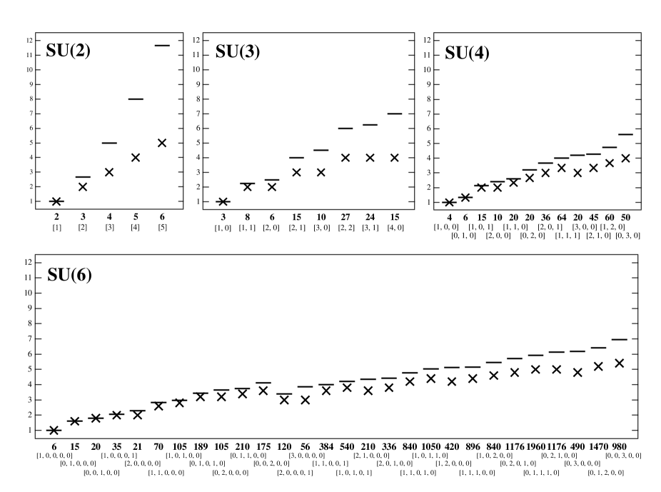
Figure 1: The systematic behavior of the ratios of string tensions, $d_{D}\equiv\sigma_{D}/\sigma_{F}$, at the Bogomol’nyi limit $\kappa=1$ (crosses) associated with color-electric charges in various $D$-dimensional representations in SU(2), SU(3), SU(4), and SU(6). The ratio of eigenvalues of quadratic Casimir operators is shown as black bars. Boldface numbers and brackets $[p_{1},p_{2},\ldots,p_{N-1}]$ denote the dimension and the Dynkin indices of each representation, respectively.

In Fig. 1 we show the systematic behavior of the ratio between string tensions,

$$d_{D}=\frac{\sigma_{D}}{\sigma_{F}}=\sum_{k=1}^{N-1}\frac{k(N-k)}{N-1}p_{k}\;,$$ (35)

for the gauge groups SU(2), SU(3), SU(4), and SU(6). In comparison, we also plot the corresponding ratio between the eigenvalues of the quadratic Casimir operator associated with the representations $D$ and $F$, $C^{(2)}(D)/C^{(2)}(F)$ (see, Appendix A). At glance, one finds that the ratio $d_{D}$ tends to approach the Casimir ratio in the large $N$ limit. This will become clearer in the Appendix A, where we observe that the leading contribution to the ratio of eigenvalues of Casimir operator for lower dimensional representations is given by

$$C^{(2)}(D)/C^{(2)}(F)\sim\sum_{k=1}^{N-1}\frac{k(N-k)}{N-1}p_{k}\;,$$ (36)

which coincides with Eq. (35).

It is amusing to note that if one evaluates the eigenvalues of quadratic Casimir operator only from off-diagonal generators, neglecting the original diagonal ones $T_{3}$, $T_{8}$, $\ldots$ , $T_{N^{2}-1}$, one gets

$$C_{\rm offdiag}^{(2)}(D)=\frac{1}{2}\sum_{k=1}^{N-1}k(N-k)p_{k}\;.$$ (37)

Here only induced diagonal generators, appearing through the commutation relations among off-diagonal generators are taken into account. Then, the ratio $C_{\rm offdiag}^{(2)}(D)/C_{\rm offdiag}^{(2)}(F)$ exactly reproduces Eq. (35). Since the DGL theory is based on the Abelian projection scheme, where the non-diagonal part of the non-Abelian gauge field is absent, one might be misled to expect that the string tension of the flux tube in this approach scales exclusively with the square of the original diagonal generators. The result shows, however, that this consideration is too naive. The flux tube energy is mainly controlled by induced diagonal generators. This clear result manifestly emerges in the Bogomol’nyi limit.

V Summary

We have formulated the [U(1)]^N-1 dual Ginzburg-Landau (DGL) theory as a low-energy effective theory of Abelian-projected SU($N$) gauge theory within a manifestly Weyl symmetric procedure. This leads to a Lagrangian density which corresponds to the sum of $N(N-1)/2$ types of U(1) dual Abelian Higgs models with $(N-2)(N-1)/2$ constraints among the dual gauge fields. We have calculated the string tensions of the flux-tube solution associated with static charges in various $D$-dimensional representations for SU($N$). This is analytically possible at the transition point from a type-I to type-II superconducting vacuum, also known as the Bogomol’nyi limit ($\kappa=1$). We have shown that the string tensions satisfy the flux counting rule. By comparing the ratio of string tensions, $d_{D}\equiv\sigma_{D}/\sigma_{F}$, with the ratio of eigenvalues of the quadratic Casimir operators, we have found that the flux-tube in the DGL theory mainly carries the information of induced diagonal generators rather than that of the original diagonal ones. This feature leads to the tendency, that $d_{D}\to C^{(2)}(D)/C^{(2)}(F)$ in the large $N$ limit.

In this paper we have concentrated on the Bogomol’nyi limit. The actual type of the dual superconducting vacuum is not determined yet, which is one of the longstanding problems in this scenario. Of course, finally it should be determined directly from the non-Abelian gauge theory. The investigation of monopole dynamics based on lattice simulations is a promising way for this purpose. In fact, such efforts for the SU(2) and the SU(3) cases are in progress Suzuki:2001tp . Once the vacuum parameters are found, it becomes interesting to compare the ratio of the string tension of the flux tubes for arbitrary sources in the DGL theory, with observed lattice data Deldar:1999vi ; Bali:2000un ; Lucini:2001nv ; DelDebbio:2001kz ; DelDebbio:2001sj in the non-Abelian theory.

Appendix A Eigenvalue of quadratic Casimir operator

The eigenvalue of quadratic Casimir operator $C^{(2)}[D]$ for arbitrary dimensional representations in SU($N$) can be expressed in terms of the Dynkin indices $[p_{1},p_{2},\ldots,p_{N-1}]$. For SU(2), SU(3), SU(4), and SU(6) cases:

$$\mbox{SU(2):}\quad C^{(2)}[D] = \frac{p_{1}}{2}+\left(\frac{p_{1}}{2}\right)^{2},$$ (38)

$$\mbox{SU(3):}\quad C^{(2)}[D] = p_{1}+p_{2}+\left(\frac{p_{1}+p_{2}}{2}\right)^{2}+\left(\frac{p_{1}-p_{2}}{2\sqrt{3}}\right)^{2},$$ (39)

$$\mbox{SU(4):}\quad C^{(2)}[D] = \frac{3}{2}(p_{1}+\frac{4}{3}p_{2}+p_{3})+\left(\frac{p_{1}+p_{2}+p_{3}}{2}\right)^{2}+\left(\frac{p_{1}+p_{2}-p_{3}}{2\sqrt{3}}\right)^{2}+\left(\frac{p_{1}-2p_{2}-p_{3}}{2\sqrt{6}}\right)^{2},$$ (40)

$$\mbox{SU(6):}\quad C^{(2)}[D] = \frac{5}{2}(p_{1}+\frac{8}{5}p_{2}+\frac{9}{5}p_{3}+\frac{8}{5}p_{4}+p_{5})+\left(\frac{p_{1}+p_{2}+p_{3}+p_{4}+p_{5}}{2}\right)^{2}$$ (41)

$$+\left(\frac{p_{1}+p_{2}+p_{3}+p_{4}-p_{5}}{2\sqrt{3}}\right)^{2}+\left(\frac{p_{1}+p_{2}+p_{3}-2p_{4}-p_{5}}{2\sqrt{6}}\right)^{2}$$

$$+\left(\frac{p_{1}+p_{2}-3p_{3}-2p_{4}-p_{5}}{2\sqrt{10}}\right)^{2}+\left(\frac{p_{1}-4p_{2}-3p_{3}-2p_{4}-p_{5}}{2\sqrt{15}}\right)^{2}.$$

These formulae can be obtained by paying attention to the highest weight state of the representation. As an example, it is instructive to learn the derivation from the SU(2) case. Let the state which belongs to $D$-dimensional representation be $|D\rangle$ and its highest weight state $|D_{\rm max}\rangle$, where the latter state is defined so as to satisfy $E_{+}|D_{\rm max}\rangle=0$ with raising operator $E_{+}\equiv T_{1}+iT_{2}$. Operating $T_{3}$ on the highest weight, we get an eigenvalue $p_{1}/2$ with the Dynkin index $[p_{1}]$:

$$T_{3}|D_{\rm max}\rangle=\frac{p_{1}}{2}|D_{\rm max}\rangle.$$ (42)

Then the eigenvalue of the quadratic Casimir operator is calculated as

$$C^{(2)}[D]=\langle D|\sum_{a=1}^{3}T_{a}T_{a}|D\rangle=\langle D_{\rm max}|E_{-}E_{+}+T_{3}+T_{3}^{2}|D_{\rm max}\rangle=\frac{p_{1}}{2}+\left(\frac{p_{1}}{2}\right)^{2}.$$ (43)

This derivation is extended straightforwardly to the SU(3), SU(4), and SU(6) cases, which provides the above expressions. The dimension $D_{N}$ for the representation $[p_{1},p_{2},\ldots,p_{N-1}]$ is

$$D_{N} = \frac{1}{2!\cdots(N-1)!}(p_{1}+1)(p_{1}+p_{2}+2)\cdots(p_{1}+\cdots+p_{N-1}+N-1)$$ (44)

$$\times(p_{2}+1)(p_{2}+p_{3}+2)\cdots(p_{2}+\cdots+p_{N-1}+N-2)$$

$$\times\cdots$$

$$\times(p_{N-2}+p_{N-1}+2)$$

$$\times(p_{N-1}+1).$$

Explicitly, this means for our cases

$$\mbox{SU(2):}\quad D_{2} = p_{1}+1,$$ (45)

$$\mbox{SU(3):}\quad D_{3} = \frac{1}{2}(p_{1}+1)(p_{1}+p_{2}+2)$$ (46)

$$\times(p_{2}+1),$$

$$\mbox{SU(4):}\quad D_{4} = \frac{1}{2!3!}(p_{1}+1)(p_{1}+p_{2}+2)(p_{1}+p_{2}+p_{3}+3)$$ (47)

$$\times(p_{2}+1)(p_{2}+p_{3}+2)$$

$$\times(p_{3}+1),$$

$$\mbox{SU(6):}\quad D_{6} = \frac{1}{2!3!4!5!}(p_{1}+1)(p_{1}+p_{2}+2)(p_{1}+p_{2}+p_{3}+3)(p_{1}+p_{2}+p_{3}+p_{4}+4)(p_{1}+p_{2}+p_{3}+p_{4}+p_{5}+5)$$ (48)

$$\times(p_{2}+1)(p_{2}+p_{3}+2)(p_{2}+p_{3}+p_{4}+3)(p_{2}+p_{3}+p_{4}+p_{5}+4)$$

$$\times(p_{3}+1)(p_{3}+p_{4}+2)(p_{3}+p_{4}+p_{5}+3)$$

$$\times(p_{4}+1)(p_{4}+p_{5}+2)$$

$$\times(p_{5}+1).$$

References

• (1) G. ’t Hooft, in High-Energy Physics. Proceedings of the EPS International Conference, Palermo, Italy, 23-28 June 1975, Vol. 2, edited by A. Zichichi (Bologna, 1976), pp. 1225–1249.
• (2) S. Mandelstam, Phys. Rept. 23C, 245 (1976).
• (3) T. Suzuki, Prog. Theor. Phys. 80, 929 (1988).
• (4) S. Maedan and T. Suzuki, Prog. Theor. Phys. 81, 229 (1989).
• (5) H. Suganuma, S. Sasaki, and H. Toki, Nucl. Phys. B435, 207 (1995), eprint hep-ph/9312350.
• (6) S. Sasaki, H. Suganuma, and H. Toki, Prog. Theor. Phys. 94, 373 (1995).
• (7) G. ’t Hooft, Nucl. Phys. B190, 455 (1981).
• (8) Z. F. Ezawa and A. Iwazaki, Phys. Rev. D25, 2681 (1982).
• (9) Z. F. Ezawa and A. Iwazaki, Phys. Rev. D26, 631 (1982).
• (10) A. S. Kronfeld, G. Schierholz, and U. J. Wiese, Nucl. Phys. B293, 461 (1987).
• (11) T. Suzuki and I. Yotsuyanagi, Phys. Rev. D42, 4257 (1990).
• (12) F. Brandstaeter, U. J. Wiese, and G. Schierholz, Phys. Lett. B272, 319 (1991).
• (13) H. Shiba and T. Suzuki, Phys. Lett. B351, 519 (1995), eprint hep-lat/9408004.
• (14) G. S. Bali, V. Bornyakov, M. Muller-Preussker, and K. Schilling, Phys. Rev. D54, 2863 (1996), eprint hep-lat/9603012.
• (15) V. Bornyakov et al., Nucl. Phys. Proc. Suppl. 106, 634 (2002), eprint hep-lat/0111042.
• (16) Y. Koma and H. Toki, Phys. Rev. D62, 054027 (2000), eprint hep-ph/0004177.
• (17) Y. Koma, E. M. Ilgenfritz, H. Toki, and T. Suzuki, Phys. Rev. D64, 011501 (2001), eprint hep-ph/0103162.
• (18) Y. Koma, E. M. Ilgenfritz, T. Suzuki, and H. Toki, Phys. Rev. D64, 014015 (2001), eprint hep-ph/0011165.
• (19) E. B. Bogomol’nyi, Sov. J. Nucl. Phys. 24, 449 (1976).
• (20) H. J. de Vega and F. A. Schaposnik, Phys. Rev. D14, 1100 (1976).
• (21) M. N. Chernodub, Phys. Lett. B474, 73 (2000), eprint hep-ph/9910290.
• (22) T. Suzuki et al., Nucl. Phys. Proc. Suppl. 106, 631 (2002), eprint hep-lat/0110059.
• (23) S. Deldar, Phys. Rev. D62, 034509 (2000), eprint hep-lat/9911008.
• (24) G. S. Bali, Phys. Rev. D62, 114503 (2000), eprint hep-lat/0006022.
• (25) B. Lucini and M. Teper, Phys. Rev. D64, 105019 (2001), eprint hep-lat/0107007.
• (26) L. Del Debbio, H. Panagopoulos, P. Rossi, and E. Vicari, Phys. Rev. D65, 021501 (2002), eprint hep-th/0106185.
• (27) L. Del Debbio, H. Panagopoulos, P. Rossi, and E. Vicari, JHEP 01, 009 (2002), eprint hep-th/0111090.
• (28) Y. Koma, M. Koma, D. Ebert, and H. Toki, Towards the string representation of the dual Abelian Higgs model beyond the London limit (2001), eprint hep-th/0108138.
• (29) Y. Koma, M. Koma, D. Ebert, and H. Toki, Effective string action for the U(1) x U(1) dual Ginzburg- Landau theory beyond the London limit (2002), eprint hep-th/0206074.