The electroweak matter sector from

an effective theory perspective

Julián Ángel Manzano Flecha

Barcelona, Juny 2002

Universitat de Barcelona

Departament d’Estructura i Constituents de la Matèria

The electroweak matter sector from

an effective theory perspective

Memòria de la tesi presentada

per Julián Ángel Manzano Flecha

per optar al grau de Doctor en Ciències Físiques

Director de tesi: Dr. Domènec Espriu

Programa de doctorat del Departament

d’Estructura i Constituents de la Matèria

“Partícules, camps i fenòmens quàntics col·lectius”

Bienni 1997-99

Universitat de Barcelona

Signat: Dr. Domènec Espriu

A Judith

Preface

This thesis deals with some theoretical and phenomenological aspects of the electroweak matter sector with special emphasis on the effective theory approach. This approach has been chosen for its versatility when general conclusions are sought without entering in the details of the currently available “fundamental” theories. Effective theories are present in the description of almost all physical phenomena even though such description is often not recognized as “effective”. In particular, effective theories in the context of quantum field theories are treated in well known works in the literature and excellent introductions are available. Because of that, I have chosen not to repeat what can be found easily elsewhere but to indicate the reader the relevant references in the introduction.

The thesis is structured in chapters that are almost in one to one correspondence with my research articles. Namely Chapter 2 is based on the article published in Phys.Rev.D60: 114035, 1999 with some typos corrected and with some notational modifications made in order to comply with the rest of the thesis notation. Chapter 3 is based on the article published in Phys.Rev.D63: 073008, 2001 where again some modifications have been made. In particular a whole section was completely omitted in favor of the next chapter which is based in a recent research article that extensively surpass the contents of that section. This article, which is the is the groundwork of Chapter 4, has been accepted for publication in Phys.Rev. and has E-Print archive number hep-ph/0204085 (in http://xxx.lanl.gov/multi). Chapter 5 is based on the publication Phys.Rev.D65: 073005, 2002 and finally Chapter 6 is based on a recent work not yet published.

At the end of the thesis I have included a set of appendices that can be useful for those interested in technical details of some sections. Even though chapters are based on research articles some changes and new sections have been inserted in order to make them more self-contained. Whenever possible I have left some of the intermediate calculational steps to the ease of those interested in reobtaining some results. In order to conform to the University rules part of the thesis has been written in Spanish. In particular the introduction and conclusion are presented in duplicate, English and Spanish.

Prefacio

Esta tesis trata aspectos teóricos y fenomenológicos del sector de materia electrodébil con especial énfasis en el uso de lagrangianos efectivos. Hemos utilizado la técnica de lagrangianos efectivos debido a la versatilidad que nos brinda a la hora de obtener resultados generales sin entrar en los detalles concretos de cada una de las teorías “fundamentales” actualmente utilizadas. Las teorías efectivas están presentes en la descripción de casi todos los fenómenos físicos aun cuando muchas veces tal descripción no es reconocida como tal. En particular el uso de teorías efectivas en el contexto de las teorías cuánticas de campos está tratado en reconocidos trabajos de la literatura científica y se dispone de excelentes introducciones. Es por ello que he preferido no repetir aquí los temas que fácilmente pueden hallarse en dichos trabajos, optando por dirigir al lector a las referencias adecuadas al comienzo de la introducción.

Esta tesis se estructura en capítulos que han sido basados en mis artículos de investigación. Concretamente, el Capítulo 2 está basado en el artículo publicado en la revista Phys.Rev.D60: 114035, 1999 con algunas correcciones tipográficas y con algunas modificaciones de notación para adaptarlo al resto de la tesis. El Capítulo 3 está basado en el artículo publicado en Phys.Rev.D63: 073008, 2001 donde también se han efectuado algunas modificaciones. En particular he omitido una sección completa ya que su antiguo contenido está ampliado y mejorado en el Capítulo 4 basado en un artículo reciente que trata el tema de manera extensiva. Este artículo ha sido aceptado para ser publicado en la revista Phys.Rev. y tiene número de archivo electrónico hep-ph/0204085 (en http://xxx.lanl.gov/multi). El Capítulo 5 está basado en la publicación en Phys.Rev.D65: 073005, 2002 y finalmente el Capítulo 6 está basado en un trabajo reciente que aún no ha sido publicado.

Al final de la tesis he incluído un conjunto de apéndices que pueden ser útiles para aquellos interesados en los detalles técnicos de algunas secciones. Aún cuando los capítulos están basados en los artículos de investigación he agregado algunas secciones para hacerlos más independientes. Además he intentado dejar pasos intermedios en algunos cálculos para facilitar la reproducción de algunos de los resultados. Cumpliendo con las normas de la Universidad parte de la tesis está escrita en castellano. En particular la introducción y las conclusiones se presentan por duplicado en inglés y en castellano.

Agradecimientos

Una tesis es algo más que una colección de trabajos, es por sobre todo una colección de experiencias. Es por ello que en esta sección quisiera volcar al menos una ínfima parte del sentimiento de gratitud que tengo hacia las personas con las que he tenido la suerte de relacionarme en este proceso. En primer lugar quisiera comenzar con mi jefe, en Domènec. “Yo hago fenomenología” me dijo cuando discutíamos las alternativas de tema de tesis. “Uff, fenomenología…, no sé…” le contesté poco convencido. “Mira, hay fenomenología y FENOMENOLOGIA” me contestó. Fue suficiente; era un alivio saber que no haría fenomenología sino FENOMENOLOGIA y con esto comencé a trabajar entusiasmado. Por supuesto ahora que he acabado no se si he hecho fenomenología o FENOMENOLOGIA, incluso la parte de TEORIA quizás sea sólo teoría. Lo que si me queda claro es que en estos años Domènec siempre me ha apoyado y me ha animado en mis frecuentes desvíos del camino señalado. Es este apoyo el que me ha hecho sentir cómodo trabajando con él y uno de los aspectos que más valoro de su papel como director. Gracias Domènec, ha sido un placer trabajar con vos.

Y por supuesto no me puedo olvidar aquí de mis compañeros de doctorado, los unos y los otros. Los unos, David, Guifré, Joan, Ignasi, Toni ahora ya doctores con los cuales comencé a pelearme con la física y con los cuales disfruté de innumerables discusiones. Los otros, Dani, Dolors, Enric, que empezaron mas tarde y que ya están acabando! Quiero agradecerles aquí los buenos momentos (¡malos no hubo!;) que pasamos entre estas venerables paredes. Enric i Dolors, Gràcies per l’ajuda en les meves cuites d’última hora!! Tampoco me quiero olvidar de los benjamines (¡que nadie se ofenda!), Alex, Aleix, Lluís, Toni, Luca, a todos les deseo que disfruten de la tesis al máximo, que todo se acaba aunque no lo parezca! Luca, Gracias por tus ideas revolucionarias, en física, política y otros asuntos que no nombraré aquí, he disfrutado mucho de tu compañía.

Algo que no quiero olvidarme de agradecer es el buen ambiente de trabajo del departamento, Joan, José Ignacio, Quim, Pere, Rolf (al menos antes de su paso a las altas esferas), Josep,… les quiero agradecer especialmente haber estado allí siempre dispuestos a aguantar y a pasarlo bien con nuestras dudas y certezas.

Pere, gràcies per l’entusiasme contagiós!

Finalmente quiero acordarme de mi familia, Má, Pá, Pablo, ¡qué les voy a agradecer! ¡¡Qué los quiero!! Y a vos Ju, que sos mi joya en esta vida, aquesta tesi és per a tu.

Resumen de la Tesis

1 Introducción

Las Teorías Cuánticas de Campos (QFT) se definen utilizando el grupo de renormalización. La idea básica tiene sus orígenes en el mundo de la materia condensada [1] y básicamente se puede expresar diciendo que en el límite termodinámico (un número infinito de grados de libertad) la integración de los grados de libertad de alta frecuencia es equivalente a una redefinición de los operadores que aparecen en la teoría. Cuando el número de dichos operadores es finito decimos que la teoría es ‘renormalizable’ y cuando no lo es decimos que es ‘no renormalizable’ o efectiva [2, 3]. Las teorías renormalizables pueden ser consideradas como Teorías Cuánticas de Campos (QFT) ‘fundamentales’ ya que el límite al continuo es posible.

En cualquier caso, los operadores renormalizados poseen una dependencia en el cut-off que regulariza la teoría. Esta dependencia está dictada principalmente por la dimensión naive del operador. Cuanto mayor es dicha dimensión, mayor es la supresión dictada por el cut-off. Por ello, las teorías no renormalizables pueden ser analizadas en la práctica truncando el número de operadores que se ordenan por dimensión creciente. Los operadores de dimensión menor dan las contribuciones más importantes a los observables de baja energía, lo cual hace que estas teorías tengan poder de predicción si nos restringimos a dicho régimen energético. A medida que incrementamos la energía o el orden en teoría de perturbaciones (relacionado con el orden en energía por el teorema de Weinberg [4]), se necesitan más y más operadores en los cálculos, y por lo tanto el poder de predicción se reduce y eventualmente la teoría se vuelve ineficaz. Esta característica (o inconveniente) de las teorías efectivas está compensada por sus ventajas en términos de generalidad. Como diferentes teorías de altas energías pertenecen a la misma clase de universalidad (la misma fenomenología a bajas energías) las teorías efectivas se pueden considerar como una forma compacta de probar diversas teorías sin entrar en sus peculiaridades irrelevantes de altas energías. Podemos resumir estas consideraciones en la Tabla (1.1)

Aparte de consideraciones dimensionales, las simetrías son el otro ingrediente básico que clasifica operadores y restringe la mezcla de los mismos generada por el grupo de renormalización.

QFT renormalizables	QFT efectivas
número finito de operadores	número infinito de operadores (truncación controlada por la dimensión)
poder de predicción a energías arbitrarias	poder de predicción a bajas energías
proliferación de modelos	generalidad

Cuadro 1.1: QFT renormalizables vs. QFT efectivas

El objetivo de esta tesis es el estudio de algunos problemas abiertos en el sector de materia electrodébil. Los temas estudiados incluyen:

• Aspectos generales de modelos de ruptura dinámica de simetría donde estudiamos posibles trazas que estos mecanismos pueden dejar a bajas energías.

• Un tratamiento general de la violación de la simetría $CP$ y la mezcla de familias en el ámbito de una teoría efectiva y la determinación de algunos de los coeficientes efectivos involucrados.

• Aspectos teóricos conectando el grupo de renormalización, la invariancia gauge, $CP$, $CPT$, y los observables físicos.

• La posibilidad de acotar experimentalmente algunos de los acoplos efectivos involucrados en el futuro acelerador de protones LHC.

En lo que sigue presentaremos un resumen detallado de los temas tratados en esta tesis.

A pesar de que la estructura básica del Modelo Estándar (SM) de las interacciones electrodébiles ya ha sido bien verificada gracias a un gran número de experimentos, su sector de ruptura de simetría no ha sido firmemente establecido aún, tanto desde el punto de vista teórico como experimental.

En la versión mínima del SM de interacciones electrodébiles, el mismo mecanismo (un único doblete escalar complejo) da masa simultáneamente a los bosones de gauge $W$ y $Z$ y a los campos de materia fermiónicos (con la posible excepción del neutrino). Este mecanismo está, sin embargo, basado en una aproximación perturbativa. Desde el punto de vista no perturbativo el sector escalar del SM mínimo se supone trivial, que a su vez es equivalente a considerar a dicho modelo como una truncación de una teoría efectiva. Esto implica que a una escala $\sim 1$ TeV nuevas interacciones deberían aparecer si el Higgs no se encuentra a más bajas energías [5]. El cut-off de 1 TeV está determinado por estudios no perturbativos y sugerido por la falta de validez del esquema perturbativo a esa escala. Por otro lado, en el SM mínimo es completamente antinatural tener un Higgs ligero ya que su masa no está protegida por ninguna simetría (el así denominado problema de jerarquías).

Esta contradicción se resuelve utilizando extensiones supersimétricas del SM, donde esencialmente tenemos el mismo mecanismo, aunque el sector escalar es mucho más rico en este caso con preferencia de escalares relativamente ligeros. En realidad, si la supersimetría resulta ser una idea útil en fenomenología, es crucial que el Higgs se encuentre con una masa $M_{H}\leq 125$ GeV, ya que si esto no ocurre los problemas teóricos que motivaron la introducción de la supersimetría reaparecerían [6]. Cálculos a dos loops [7] elevan este límite a alrededor de los 130 GeV.

Una tercera posibilidad es la dada por modelos de ruptura dinámica de la simetría (tales como la teorías de technicolor (TC) [8]). En este caso existen interacciones que se vuelven fuertes, típicamente a la escala $\Lambda_{\chi}\simeq 4\pi v$ ($v=250$ GeV), rompiendo la simetría global $SU(2)_{L}\times SU(2)_{R}$ a su subgrupo diagonal $SU(2)_{V}$ y produciendo bosones de Goldstone que eventualmente pasan a ser los grados de libertad longitudinales de $W^{\pm}$ y $Z$. Para transmitir esta ruptura de simetría a los campos ordinarios de materia se requiere de interacciones adicionales, usualmente denominadas technicolor extendido (ETC) y caracterizado por una escala diferente $M$. Generalmente, se asume que $M\gg 4\pi v$ para mantener bajo control a posibles corrientes neutras de cambio de sabor (FCNC) [9]. Así, una característica distintiva de estos modelos es que el mecanismo responsable de dar masas a los bosones $W^{\pm}$ y $Z$ y a los campos de materia es diferente.

¿Dónde estamos actualmente? Algunos irian tan lejos como para decir que un Higgs elemental (supersimétrico o de otro tipo) ha sido ‘visto’ a través de correcciones radiativas y que su masa es menor que 200 GeV, o incluso que ha sido descubierto en los últimos días del LEP con una masa $\simeq$115 GeV [10]. Otros descreen de estas afirmaciones (ver por ejemplo [11] para un estudio crítico sobre las actuales afirmaciones acerca de un Higgs ligero).

El enfoque basado en los Lagrangianos efectivos ha sido notablemente útil a la hora de fijar restricciones al tipo de nueva física detrás del mecanismo de ruptura de simetría del SM tomando como datos básicamente los resultados experimentales de LEP [12] (y SLC [13]). Hasta ahora ha sido aplicado principalmente al sector bosónico, las así denominadas correcciones ’oblicuas’. La idea es considerar el Lagrangiano más general que describe las interacciones entre el sector de gauge y los bosones de Goldstone que aparecen luego de que la ruptura $SU(2)_{L}\times SU(2)_{R}\rightarrow SU(2)_{V}$ tiene lugar. Ya que no se asume ningún mecanismo especial para esta ruptura, el procedimiento es completamente general asumiendo, por supuesto, que las partículas no explícitamente incluidas en el Lagrangiano efectivo son mucho más pesadas que las que sí lo están. La dependencia en el modelo específico tiene que estar contenida en los coeficientes de los operadores de dimensión más alta.

Con la idea de extender este enfoque que ha sido tan eficaz, en el Capítulo 2 parametrizamos, independientemente del modelo, posibles desviaciones de las predicciones del Modelo Estándar mínimo en el sector de materia. Como ya hemos dicho, esto se realiza asumiendo sólo el esquema de ruptura de simetría del Modelo Estándar y que las partículas aún no observadas son suficientemente pesadas, de manera que la simetría está realizada de manera no lineal. También reexaminamos, dentro del lenguaje de las teorías efectivas, hasta que punto los modelos más simples de ruptura dinámica están realmente acotados y las hipótesis utilizadas en la comparación con el experimento. Ya que los modelos de ruptura dinámica de simetría pueden ser aproximados a energías intermedias $\Lambda_{\chi}<E<M$ por operadores de cuatro fermiones, presentamos una clasificación completa de los mismos cuando las nuevas partículas aparecen en la representación usual del grupo $SU(2)_{L}\times SU(3)_{c}$ y también una clasificación parcial en el caso general. Luego discutimos la precisión de la descripción basada en operadores de cuatro fermiones efectuando el matching con una teoría ‘fundamental’ en un ejemplo simple. Los coeficientes del Lagrangiano efectivo en el sector de materia para los modelos de ruptura dinámica de simetría (expresados en términos de los coeficientes de los operadores de cuatro fermiones) son luego comparados con aquellos provenientes de modelos con escalares elementales (como el Modelo Estándar mínimo). Contrariamente a lo creído comúnmente, observamos que el signo de las correcciones de vértice no están fijadas en los modelos de ruptura dinámica de simetría. Resumiendo, sin analizar los temas de violación de $CP$ o fenomenología de mezcla de familias, el trabajo de este capítulo proporciona las herramientas teóricas requeridas para analizar en términos generales restricciones en el sector de materia del Modelo Estándar.

Hasta aquí nada definitivo se ha dicho acerca de la violación de $CP$ o la mezcla de familias. Sin embargo, tal como sucede en el SM, estos fenómenos están probablemente relacionados con el sector de ruptura de simetría.

La violación de $CP$ y la mezcla de familias se encuentran entre los enigmas más intrigantes del SM. La comprensión del origen de la violación de $CP$ es en realidad uno de los objetivos más importantes de los experimentos actuales y futuros. Esto está completamente justificado ya que dicha comprensión puede no sólo revelar características inesperadas de sectores de nueva física, sino también dar pistas en el entendimiento de aspectos fenomenológicos complejos como la bariogénesis en cosmología.

En el Modelo Estándar mínimo la información sobre las cantidades que describen esta fenomenología está codificada en la matriz de mezcla de Cabibbo-Kobayashi-Maskawa (CKM) (aquí denotada $K$). En este contexto, aunque la matriz de masas más general posee, en principio, un gran número de fases, sólo las matrices de diagonalización de fermiones de quiralidad left sobreviven combinadas en una única matriz CKM. Esta matriz contiene sólo una fase compleja observable. Si esta única fuente de violación de $CP$ es suficiente o no para explicar nuestro mundo es, actualmente, una incógnita.

Como es bien sabido, algunas de las entradas de esta matriz están muy bien medidas, mientras que otras (tales como $K_{tb}$, $K_{ts}$ y $K_{td}$) son poco conocidas y la única restricción experimental real viene dada por los requerimientos de unitariedad. En este problema en particular se ha invertido un gran esfuerzo en la última década y esta dedicación continuará en el futuro inmediato destinada a lograr en el sector cargado una precisión comparable con la lograda en el sector neutro. Como guía, mencionamos que la precisión en $\sin 2\beta$ se espera que sea superior al 1 % en el futuro LHCb, y una precisión semejante se espera para ese momento en los experimentos actualmente en curso (BaBar, Belle) [14].

Unos de los propósitos de los experimentos de nueva generación es testear la ‘unitariedad de la matriz CKM’. Puesto de esta forma, dicho propósito no parece tener mucho sentido. Por supuesto si sólo mantenemos las tres generaciones conocidas, la mezcla ocurre a través de una matriz de $3\times 3$ que es, por construcción, necesariamente unitaria. Lo que realmente se quiere decir con la afirmación anterior es que se quiere verificar si los elementos de matriz $S$ observables, que a nivel árbol son proporcionales a elementos de CKM, cuando son medidos en decaimientos débiles están o no de acuerdo con las relaciones de unitariedad a nivel árbol predichas por el Modelo Estándar. Si escribimos por ejemplo

$$\left\langle q_{j}\left|W_{\mu}^{+}\right|q_{i}\right\rangle=U_{ij}V_{\mu},$$ (.1)

a nivel árbol, está claro que la unitariedad de la matriz CKM implica

$$\sum_{k}U_{ik}U_{jk}^{\ast}=\delta_{ij},$$ (.2)

Sin embargo, incluso si no existe nueva física más allá del Modelo Estándar las correcciones radiativas contribuyen a los elementos de matriz relevantes en los decaimientos débiles y arruinan la unitariedad de la ‘matriz CKM’ $U$, en el sentido de que los correspondientes elementos de matriz $S$ no estarán restringidos a obedecer las relaciones de unitariedad indicadas arriba. Obviamente, las desviaciones de unitariedad debidas a las correcciones radiativas electrodébiles serán necesariamente pequeñas. Después veremos a que nivel debemos esperar violaciones de unitariedad debidas a correcciones radiativas.

Pero por supuesto, las violaciones de unitariedad que realmente son interesantes son las causadas por nueva física. La física más allá del Modelo Estándar se puede manifestar de diferentes maneras y a diferentes escalas. Otra vez, tal como hemos hecho con el caso sin mezcla ni violación de $CP$ asumiremos que la nueva física puede aparecer a una escala $\Lambda$ que es relativamente grande comparada con $M_{Z}$. Esta observación incluye al sector escalar también; es decir, asumimos que el Higgs —si es que existe— es suficientemente pesado. Con estas hipótesis trataremos de extraer algunas conclusiones acerca de la mezcla de familias y la violación de $CP$ utilizando técnicas de Lagrangianos efectivos.

Ilustremos esta idea con un ejemplo simple: Supongamos el caso en el que hay una nueva generación pesada. En ese caso podemos proceder de dos maneras. Una posibilidad consiste en tratar a todos los fermiones, ligeros o pesados, al mismo nivel. Terminaríamos entonces con una matriz de mezcla de $4\times 4$ unitaria, cuya submatriz de $3\times 3$, correspondiente a los fermiones ligeros, no necesitaría ser —y en realidad no sería— unitaria. Puesto de esta manera, las desviaciones de unitariedad (¡incluso a nivel árbol!) podrían ser considerables. La manera alternativa de proceder consistiría, de acuerdo a la filosofía de los Lagrangianos efectivos, en integrar completamente a la generación pesada. Nos quedaríamos entonces, al nivel más bajo en la expansión en la inversa de la masa pesada, con los términos cinéticos y de masa ordinarios para los fermiones ligeros y una matriz de mezcla ordinaria de $3\times 3$ que sería obviamente unitaria. Naturalmente no existe contradicción lógica entre ambos procedimientos ya que lo que realmente importa es el elemento matriz $S$ y este adquiere, si seguimos el segundo procedimiento (integración de campos pesados), dos clases de contribuciones: una de los operadores de dimensión más baja, que contienen sólo fermiones ligeros, y otra de los de dimensión más alta obtenidos después de integrar los campos pesados. El resultado para el elemento de matriz $S$ observable debe ser el mismo sea cual sea el procedimiento aplicado, pero del segundo método aprendemos que las violaciones de unitariedad en el triángulo de tres generaciones están suprimidas por una masa pesada. Este simple ejercicio ilustra las ventajas del enfoque basado en los Lagrangianos efectivos.

En el Capítulo 3 extendemos el Lagrangiano efectivo presentado en el Capítulo 2 para considerar mezcla de familias y violación de $CP$. Este Lagrangiano contiene los operadores efectivos que dan la contribución dominante en teorías donde la física más allá del Modelo Estándar aparece a la escala $\Lambda>>M_{W}$. Como en el Capítulo 2 aquí mantenemos sólo los operadores efectivos no universales dominantes, o sea los de dimensión cuatro. Como no hacemos otras suposiciones aparte de las de simetría, consideramos términos cinético y de masa no diagonales y efectuamos con toda generalidad la diagonalización y el paso a la base física. Esta diagonalización no deja trazas en el SM aparte de la matriz CKM. Sin embargo, veremos aquí que mucha más información de la base débil queda en los operadores efectivos escritos en la base diagonal. Luego determinaremos la contribución en diferentes observables y discutiremos las posibles nuevas fuentes de violación de $CP$, la idea es extraer conclusiones sobre nueva física más allá del Modelo Estándar de consideraciones generales, sin tener que calcular en cada modelo. En el mismo capítulo presentamos los valores de los coeficientes del Lagrangiano efectivo calculados en algunas teorías, incluido el Modelo Estándar con un Higgs pesado, y tratamos de obtener conclusiones generales sobre el esquema general exhibido por la física más allá del Modelo Estándard en lo que concierne a la violación de $CP$.

En el proceso tenemos que tratar un problema teórico que es interesante por sí mismo: la renormalización de la matriz CKM y de la función de onda (wfr.) en el esquema on-shell en presencia de mezcla de familias. Pero, ¿por qué tenemos que preocuparnos de la wfr. o de los contra-términos de CKM si aquí trabajamos a nivel árbol? La respuesta es bastante simple: incluso a nivel árbol uno de los operadores efectivos contribuye a las autoenergías fermiónicas y por lo tanto a las wfr. Esto implica que esta contribución “indirecta” tiene que ser tenida en cuenta ya que para calcular observables físicos las wfr. están dictadas por los requerimientos de LSZ que a su vez son equivalentes a los requerimientos del esquema on-shell. Además, se puede ver que los contra-términos de CKM están también relacionados con las wfr. (aunque no con las físicas o “externas”) y por lo tanto otra contribución potencial puede aparecer a través de este contra-término.

En este punto descubrimos que algunas preguntas acerca de la correcta implementación del esquema on-shell en presencia de mezcla de familias quedaban por contestar. Algunas de estas preguntas fueron hechas por primera vez en [15] donde se presentaron supuestas inconsistencias entre el esquema on-shell y la invariancia gauge. Motivados por estos resultados decidimos investigar el tema del esquema on-shell en presencia de mezcla de familias y su relación con la invariancia gauge. Nuestro trabajo en relación con este tema está presentado en el Capítulo 4 y los resultados de este capítulo se utilizan en el caso mucho más simple de la contribución de teoría efectiva a primer orden. Aquí vale la pena remarcar que los resultados obtenidos en el Capítulo 4 van mucho más allá que su aplicación en el Capítulo 3 y son relevantes en los cálculos de violación de $CP$ en futuros experimentos de alta precisión.

Hagamos aquí una breve introducción al problema: Cuando calculamos una amplitud física de vértice a nivel 1-loop tenemos que considerar las contribuciones de nivel árbol más correcciones de varios tipos. O sea, necesitamos contra-términos para la carga eléctrica, ángulo de Weinberg y renormalización de la función de onda del bosón de gauge $W$. También necesitamos la wfr. de los fermiones externos y los contra-términos de CKM. Estas últimas renormalizaciones están relacionadas en una forma que veremos en el Capítulo 4 [16]. Finalmente necesitamos calcular los diagramas 1PI correspondientes al vértice en cuestión.

Hasta aquí todo lo dicho es.estándar. Sin embargo, una controversia relativamente antigua existe en la literatura con respecto a cuál es la manera adecuada de definir las wfr. externas y los contra-términos de CKM. La cuestión es bastante compleja ya que estamos tratando con partículas que son inestables (y por lo tanto las autoenergías, relacionadas con las wfr., desarrollan cortes en el plano complejo que en general dependen de la fijación de gauge) y con la cuestión de mezcla de familias.

Varias propuestas han aparecido en la literatura tratando de definir los contra-términos adecuados tanto para las patas externas (wfr.) como para los elementos de matriz de CKM. Las condiciones on-shell que diagonalizan el propagador fermiónico on-shell fueron introducidas originalmente en [17]. En [18] las wfr. que “satisfacían” las condiciones de [17] fueron derivadas. Sin embargo en [18] no se tenía en cuenta la presencia de cortes en las autoenergías, un hecho que entra en conflicto con las condiciones en [17]. Más tarde esto fue reconocido en [19]. El problema se puede resumir diciendo que las condiciones on-shell definidas en [17] son en realidad imposibles de satisfacer por un conjunto mínimo de constantes de renormalización debido a la presencia de partes absortivas en las autoenergías. El autor de [19] evita este problema introduciendo una prescripción que elimina de facto estas partes absortivas, pero pagando el precio de no diagonalizar el propagador fermiónico en sus índices de familia.

Las identidades de Ward basadas en la simetría de gauge SU(2)_L relacionan las wfr. y los contra-términos de CKM [16]. En [15] se muestra que si la prescripción de [18] se utiliza en los contra-términos de CKM, el resultado del cálculo de un observable físico resulta dependiente del parámetro de gauge. Como ya hemos mencionado, los resultados en [18] no tratan adecuadamente las partes absortivas presentes en las autoenergías; que a su vez resultan ser dependientes del parámetro de gauge. En el Capítulo 4 veremos que a pesar de los problemas existentes en la prescripción dada en [18], las conclusiones dadas en [15] son correctas: una condición necesaria para la invariancia gauge de las amplitudes físicas es que el contra-término de CKM sea independiente del parámetro de gauge. Tanto el contra-término de CKM propuesto [15] como los propuestos en [16], [20] satisfacen dicha condición.

Existen en la literatura otras propuestas para definir la renormalización de CKM, [20], [21] y [22]. En todos estos trabajos, o se utilizan las wfr. propuestas originalmente en [18] o las dadas en [19], o la cuestión de la correcta definición de la wfr. externas se evita completamente. En cualquier caso las partes absortivas de las autoenergías no son tenidas en cuenta (incluso las partes absortivas de los diagramas 1PI son evitadas en [21]). Como veremos, hacer esto conduce a amplitudes físicas —elementos de matriz $S$ — que son dependientes del parámetro de gauge, independientemente del método utilizado para renormalizar $K_{ij}$ siempre que la redefinición de $K_{ij}$ sea independiente del gauge y preserve unitariedad.

Debido a la estructura de los cortes absortivos resulta que, sin embargo, la dependencia en el parámetro de gauge en la amplitud —elemento de matriz $S$— , usando la prescripción de [19], cancela en el modulo cuadrado de la misma en el SM. Esta cancelación ha sido verificada numéricamente por los autores de [23]. En el Capítulo 4 presentaremos los resultados analíticos que muestran que esta cancelación es exacta. Sin embargo la dependencia en el parámetro de gauge permanece en la amplitud.

¿Es esto aceptable? Creemos que no. Los diagramas que contribuyen al mismo proceso físico fuera del sector electrodébil del SM pueden interferir con la amplitud del SM y revelar la inaceptable dependencia gauge. Más aún, las partes absortivas independientes del gauge están también eliminadas en la prescripción en [19]. Sin embargo, estas partes, a diferencia de las dependientes del gauge, no desaparecen de la amplitud al cuadrado tal como veremos. Además, no debemos olvidar que el esquema en [19] no diagonaliza correctamente los propagadores en sus índices de familia. El Capítulo 4 está dedicado a respaldar las afirmaciones anteriores.

En resumen, en el Capítulo 4, con la ayuda de un uso extensivo de las identidades de Nielsen [24, 25, 26] complementadas con cálculos explícitos, corroboramos que el contra-término de CKM tiene que ser independiente del parámetro de gauge y demostramos que la prescripción comúnmente utilizada para la renormalización de la función de onda conduce a amplitudes físicas dependientes del parámetro de gauge, incluso si el contra-término de CKM no depende del parámetro de gauge tal como se requiere. Para aquellos lectores no familiarizados con las identidades de Nielsen presentamos un resumen pedagógico de las mismas indicando las referencias relevantes. Usando esta tecnología mostramos que una prescripción que cumple los requerimientos de LSZ conduce a amplitudes independientes del parámetro de gauge. Las renormalizaciones de función de onda resultantes necesariamente poseen partes absortivas. Por ello verificamos explícitamente que dicha presencia no altera los requerimientos esperados en cuanto a $CP$ y $CPT$. Los resultados obtenidos utilizando esta prescripción son diferentes (incluso a nivel del módulo cuadrado de la amplitud) de los que se obtienen despreciando las partes absortivas en el caso del decaimiento del quark top. Mostramos asimismo que esta diferencia es numéricamente relevante.

Una vez que estos aspectos teóricos están aclarados pasamos al estudio de la fenomenología capaz de probar la física del sector de corrientes cargadas que es el sector sensible a la violación de $CP$ en el Modelo Estándar. Cuando nos centramos en interacciones que involucran a los bosones $W,Z$, los operadores presentes en el Lagrangiano efectivo electrodébil inducen vértices efectivos que acoplan los bosones de gauge con los campos de materia [29]

$$-\frac{e}{4c_{W}s_{W}}\bar{f}\gamma^{\mu}\left(\kappa_{L}^{NC}L+\kappa_{R}^{NC}R\right)Z_{\mu}f-\frac{e}{s_{W}}\bar{f}\gamma^{\mu}\left(\kappa_{L}^{CC}L+\kappa_{R}^{CC}R\right)\frac{\tau^{-}}{2}W_{\mu}^{+}f+h\mathchar 46\relax c\mathchar 46\relax$$ (.3)

Otros posibles efectos no son físicamente observables, tal como veremos en el Capítulo 5. En términos prácticos, LHC establecerá restricciones en los acoplos efectivos del vértice del $W$, y por lo tanto en la nueva física que contribuye a los mismos. Nuestros resultados son también relevantes en un contexto fenomenológico más amplio como una manera de restringir $\kappa_{L}$ y $\kappa_{R}$ (incluyendo nueva física y correcciones radiativas), sin necesidad de apelar a un Lagrangiano efectivo subyacente que describa un modelo específico de ruptura de simetría. Por supuesto en ese caso se pierde el poder de un Lagrangiano efectivo, es decir, se pierde el conjunto bien definido de reglas de contaje y la capacidad de relacionar diferentes procesos.

Como ya hemos destacado, incluso en el Modelo Estándar mínimo, las correcciones radiativas inducen modificaciones en los vértices. Asumiendo una dependencia suave en los momentos externos estos factores de forma pueden ser expandidos en potencias de momentos. Al orden más bajo en la expansión en derivadas, el efecto de las correcciones radiativas puede ser codificado en los vértices efectivos $\kappa_{L}$ y $\kappa_{R}$. Así, estos vértices efectivos toman valores bien definidos, valores calculables en el Modelo Estándar mínimo, y cualquier desviación de los mismos (que, incidentalmente, no han sido determinados completamente en el Modelo Estándar aún) indicaría la presencia de nueva física en el sector de materia. La capacidad que LHC tiene para fijar restricciones directas en los vértices efectivos, en particular en aquellos que involucran a la tercera generación, es de vital importancia para acotar los posibles modelos de física más allá del Modelo Estándard. El trabajo del Capítulo 5 está dedicado a este análisis en procesos cargados involucrando al quark top en el LHC.

A la energía de LHC (14 Tev) el mecanismo dominante en la producción de tops, con una sección eficaz de 800 pb [30], es el mecanismo de fusión gluon-gluon. Este mecanismo no tiene nada que ver con el sector electrodébil y por lo tanto no el más adecuado para nuestros propósitos. Aunque es el mecanismo que más tops produce y por lo tanto es importante considerarlo a la hora de estudiar los acoplos del top a través de su decaimiento, que será nuestro principal interés en el Capítulo 6, y también como background al proceso que nos ocupará en este capítulo.

Figura 1.1: Diagramas de Feynman que contribuyen al subproceso de producción de un single-top. En este caso tenemos un quark $d$ como quark espectador

Figura 1.2: Diagramas de Feynman que contribuyen al subproceso de producción de un single-top. En este caso tenemos un quark $\bar{u}$ como quark espectador

La física electrodébil entra en juego en la producción de single-top (un único top). (para una revisión reciente ver e.g. [31].) A las energías de LHC el subproceso electrodébil dominante (de lejos) que contribuye a la producción de single-top está dado por un gluon ($g$) viniendo de un protón y un quark o anti-quark ligero viniendo del otro (este proceso también se denomina de producción en canal t [32, 33]). Este proceso está graficado en las Figs. 1.1 y 1.2, donde quarks ligeros de tipo $u$ o antiquarks ligeros de tipo $\bar{d}$ son extraídos del protón, respectivamente. Estos quarks luego radian un $W$ cuyo acoplo efectivo es el objeto de nuestro interés. La sección eficaz total para este proceso en el LHC ha sido calculada en 250 pb [33], a ser comparada con los 50 pb para la asociada a la producción con un bosón $W^{+}$ y un quark $b$ extraído del mar de protón, y 10 pb que corresponden a la fusión quark-quark (producción en canal s que será analizada en el Capítulo 6). En el Tevatron (2 GeV) la sección eficaz de producción para fusión $W$-gluon es de 2.5 pb, y por lo tanto, en comparación, la producción de tops en este subproceso en particular es realmente copiosa en LHC. La simulaciones de Monte Carlo incluyendo el análisis de los productos de decaimiento del top indican que este proceso puede ser analizado en detalle en LHC y tradicionalmente ha sido considerado como el más importante para nuestros propósitos.

En una colisión protón protón también se produce un par bottom anti-top a través de un subproceso análogo. En cualquier caso los resultados cualitativos son muy similares a aquellos correspondientes a la producción de tops, de donde las secciones eficaces pueden ser fácilmente derivadas haciendo los cambios adecuados.

En el contexto de teorías efectivas, la contribución de operadores de dimension cinco a la producción de tops a través de fusión de bosones vectoriales longitudinales fue estimada hace algún tiempo en [34], aunque el estudio no fue de ningún modo completo. Debe ser mencionado que la producción de un par $t,\bar{t}$ a través de este mecanismo está muy enmascarada por el mecanismo dominante que es la fusión gluon-gluon, mientras que la producción de single-top, a través de fusión $WZ$, se supone mucho más suprimida comparada con el mecanismo presentado en este trabajo. Esto se debe a que los dos vértices son electrodébiles en el proceso discutido en [34], y a que los operadores de dimensión cinco se suponen suprimidos por una escala elevada. La contribución de operadores de dimensión cuatro no ha sido, por lo que sabemos, considerada anteriormente, aunque la capacidad de la producción de single-top para medir el elemento de matriz de CKM $K_{tb}$, ha sido hasta cierto punto analizado en el pasado (ver por ejemplo [33, 35]).

Para resumir, en el Capítulo 5 analizamos la sensibilidad de diferentes observables a la magnitud de los coeficientes efectivos que parametrizan la nueva física más allá del Modelo Estándar. También mostramos que los observables relevantes para la distinción de los acoplos quirales left y right involucra, en la práctica, la medición del espín del top que sólo puede ser realizada de forma indirecta midiendo la distribución angular de sus productos de decaimiento. Mostramos que la presencia de acoplos efectivos de quiralidad right implican que el top no se encuentra en un estado puro y que existe una única base de espín útil para conectar la distribución de los productos de decaimiento del top con la sección eficaz diferencial de producción de tops polarizados. Presentamos además las expresiones analíticas completas, incluyendo acoplos efectivos generales, de las secciones eficaces diferenciales correspondientes a los subprocesos de producción de single-top polarizado en canal t. La masa del quark bottom, que resulta ser más relevante de lo que se puede esperar, se mantiene en todo el cálculo. Finalmente analizamos diferentes aspectos de la sección eficaz total relevantes para la detección de nueva física a través de los acoplos efectivos. También hemos desarrollado la aproximación llamada de W efectivo para este proceso pero los resultados no se presentan en esta tesis [36].

Finalmente en el Capítulo 6 estudiamos un aspecto de la producción de tops que no fue finalizado en el capítulo anterior; la “medición” del espín del top a través de sus productos de decaimiento. El análisis numérico de la sensibilidad de los diferentes observables al acoplo right $g_{R}$ se realiza aquí incluyendo los productos de decaimiento del top. Ya que el principal objetivo de este capítulo es aclarar el rol del espín del top cuando el decaimiento del top también se considera, estudiamos la producción de single-top a través del canal s, más simple de analizar desde el punto de vista teórico. La producción y decaimiento del top en este canal se grafica en la Fig. (1.3)

En el Capítulo 6 mostramos como la sección eficaz diferencial correspondiente al proceso de la Fig. (1.3) se calcula en dos pasos usando la aproximación resonancia estrecha teniendo en cuenta el espín del top. O sea, en primer lugar calculamos la probabilidad de producir tops con una dada polarización y luego convolucionamos dicha probabilidad con la probabilidad de decaimiento, sumando sobre las dos polarizaciones del top. Exponemos los argumentos que permiten demostrar que los efectos de interferencia cuánticos pueden ser minimizados con una elección adecuada de la base de espín. Presentamos expresiones explícitas tanto para el canal s como para el canal t de la base de espín que diagonaliza la matriz densidad del top. En el caso del canal s utilizamos esta base en nuestro programa de integración de Monte Carlo analizando numéricamente la sensibilidad de nuestros resultados ante cambios de la base de espín o incluso ante la posibilidad de prescindir del espín completamente. Estos estudios numéricos muestran que la implementación de la base correcta de espín es importante a nivel del 4 %. Además de la cuestión del espín del top, nuestros resultados numéricos muestran claramente el papel crucial de elegir configuraciones cinemáticas concretas para los productos de decaimiento del top que maximicen la sensibilidad al acoplo $g_{R}$ tanto en magnitud como en fase.

Figura 1.3: Diagrama de Feynman correspondiente a la producción y decaimiento de single-top en el canal s.

En los apéndices de esta tesis hemos incluído material técnico que complementa los contenidos de los capítulos y algunos cálculos que pueden servir al lector interesado en reproducir los resultados. En particular hemos incluído el cálculo completo de todas las autoenergías fermiónicas en un gauge arbitrario $R_{\xi}$ .

2 Resultados y Conclusiones

En lo que sigue presentamos un sumario de los principales resultados y conclusiones de esta tesis.

• En el Capítulo 2:

  • Ofrecemos una clasificación completa de los operadores de cuatro campos fermiónicos responsables de dar masa a fermiones físicos y a bosones gauge vectoriales en modelos con rotura dinámica de simetría. Dicha clasificación se realiza cuando las nuevas partículas aparecen en las representaciones usuales del grupo $SU(2)_{L}\times SU(3)_{c}$. En el caso general discutimos, además, una clasificación parcial. Debido a que se ha tomado únicamente el caso de una sola familia, el problema de mezcla no ha sido aquí considerado.

  • Investigamos las consecuencias fenomenológicas para el sector electrodébil neutro en dicha clase de modelos. Para ello realizamos el matching entre la descripción mediante términos de cuatro fermiones y una teoría a más bajas energías que contiene sólamente los grados de libertad del SM (a excepción del Higgs). Los coeficientes de este Lagrangiano efectivo de bajas energías para modelos con rotura dinámica de simetría son, a continuación, comparados con los de modelos con escalares elementales (como por ejemplo, en el Modelo Estándar mínimo).

  • Determinamos el valor del acoplamiento efectivo de $Zb\bar{b}$ en modelos con rotura dinámica de simetría verificando que su contribución es importante, pero su signo no está determinado contrariamente a afirmaciones anteriores. El valor experimental actual se desvía del predicho por el SM en casi 3 $\sigma$. Estimamos también los efectos en los fermiones ligeros, a pesar de que no son observables actualmente. Algunas consideraciones generales concernientes al mecanismo de rotura dinámica de simetría son presentadas.

• En el Capítulo 3:

  • Analizamos la estructura de los operadores efectivos de cuatro dimensiones para el sector de materia de la teoría electrodébil cuando se permiten violaciones $CP$ y mezcla de familias.

  • Realizamos la diagonalización de los términos de masa y cinéticos demostrando que, además de la presencia de la matriz CKM en el vértice cargado del SM, aparecen nuevas estructuras en los operadores efectivos construídos con fermiones de quiralidad left. En particular la matriz CKM se encuentra también presente en el sector neutro.

  • Calculamos también la contribución de los operadores efectivos en el SM mínimo con un Higgs pesado y en el SM con un doblete de fermiones pesados adicional.

  • En general, incluso si la física responsable de la generación de los operadores efectivos adicionales conserva $CP$, las fases presentes en los acoplamientos Yukawa y cinéticos se hacen observables en los operadores efectivos tras su diagonalización.

• En el Capítulo 4:

  • Presentamos y resolvemos la cuestión sobre la definición de un conjunto de constantes wfr. a 1 loop consistentes con los requerimientos de on-shell y la invariancia gauge de las amplitudes físicas electrodébiles. Demostramos, utilizando las identidades de Nielsen, que con nuestro conjunto de constantes wfr. y una renormalización del CKM independiente del gauge, se obtienen unas amplitudes físicas para el decaimiento del top y del W independientes del gauge.

  • Mostramos que la prescripción on-shell dada en [19] no diagonaliza el propagador en los índices de familia y que dicha prescripción origina amplitudes que dependen del gauge, aunque dicha dependencia desaparece en módulo de la amplitud correspondiente al vértice cargado electrodébil. El hecho de que sólo el módulo de las amplitudes electrodébiles no dependa del gauge no es satisfactorio, ya que la interferencia con fases fuertes puede, por ejemplo, originar una dependencia gauge inaceptable. En el caso del decaimiento del top encontramos que la diferencia numérica entre nuestro resultado para el módulo al cuadrado de la amplitud y el mismo obtenido con la prescripción dada en [19] llega al $0{,}5\leavevmode\,\%{}$. Esta diferencia será relevante en los futuros experimentos de precisión diseñados para determinar el vértice $tb$.

  • Comprobamos la consistencia de nuestro esquema con el teorema $CPT$. Dicha comprobación se hace mostrando que, aunque nuestras constantes wfr. no verifican la condición de pseudo-hermiticidad ($\bar{Z}\neq\gamma^{0}Z^{\dagger}\gamma^{0}$), la anchura total de partículas y anti-partículas coincide.

• En el Capítulo 5:

  • Presentamos un cálculo completo de las secciones eficaces en el canal t para tops o anti-tops polarizados incluyendo acoplamientos efectivos right y contribuciones a la masa del quark bottom.

  • Realizamos una simulación Monte Carlo de la producción de single-top polarizado en el LHC para una colección de distribuciones en $p_{T}$ y distribuciones angulares para los quarks $t$ y $\bar{b}$. Mostramos, sin tener en cuenta backgrounds o el efecto del decaimiento del top, que podemos esperar una sensibilidad de 2 desviaciones estándar para variaciones de $g_{R}$ del orden de $5\times 10^{-2}$.

  • Mostramos, basándonos en consideraciones teóricas, que el top no puede producirse en un estado de espín puro si $g_{R}\neq 0$. Más aún, indicamos cual es la base de espín adecuada para convolucionar la sección eficaz de producción del top con la sección eficaz de decaimiento del mismo. Dicha convolución se efectúa para poder calcular el proceso completo en el marco de la aproximación de resonancia estrecha.

• En el Capítulo 6:

  • Presentamos un cálculo completo de la sección eficaz en el canal s de producción de single-top incluyendo su decaimiento. Los cálculos incluyen acoplamientos efectivos right y contribuciones de la masa del quark bottom.

  • Efectuamos una simulación Monte Carlo de la producción y decaimiento de tops polarizados en el LHC en el canal s. Representamos gráficamente diferentes distribuciones de $p_{T}$, masa invariante y distribuciones angulares construídas con los momentos del anti-leptón y el momento de los jets del bottom y del anti-bottom. Encontramos que las variaciones de $g_{R}$ del orden $5\times 10^{-2}$ son visibles con señales comprendidas entre 3 y 1 desviaciones estándar dependiendo de la fase de $g_{R}$ y de los observables elegidos.

  • Presentamos expresiones explícitas para los canales t y s de la base de espín del top que diagonaliza su matriz densidad. Comprobamos numéricamente que para el canal s dicha base minimiza los términos de interferencia ignorados en la aproximación de resonancia estrecha.

Chapter 1 Introduction

Quantum field theories (QFT) are defined through the renormalization group. The basic idea has its origins in the condensed matter world [1] and briefly can be stated by saying that in the thermodinamic limit (an infinite number of degrees of freedom) the integration of high frequency degrees of freedom can be seen as a redefinition of the operators appearing in the theory. When the number of such operators is finite we call this theory ‘renormalizable’ and when it is not we call it non-renormalizable or effective theory [2, 3]. Renormalizable theories are in principle capable of being considered as ‘fundamental’ QFT since the continuum limit is feasible.

In any case renormalized operators bear dependence on the cut-off that regularizes the theory. Such dependence is dictated mainly by the naive dimension of the operator. The bigger the dimension the bigger the cut-off suppression. Because of that, non renormalizable theories can be analyzed in practice truncating the number of operators which are ordered by increasing dimensionality. Lower dimensional operators provide the leading contribution to observables at low energies and because of that these theories still have predictive power if we restrict ourselves to such regime. As we increase the energy or the order in perturbation theory (related to the energy counting by the Weinberg theorem [4]) more and more operators are needed in calculations and therefore the predictive power reduces and eventually the theory becomes worthless. This inconvenient feature of effective theories is compensated by their advantage in terms of generality. Since different high energy models belong to the same universality class (the same phenomenology at low energies) effective field theories provide a way to probe theories in a compact way without entering in irrelevant high energy features. In total we can summarize these considerations in Table (1.1)

renormalizable QFT	effective QFT
finite number of operators	infinite number of operators (truncation controlled by dimensionality)
predictability power at all energies	predictability power at low enegies
model proliferation	generality

Table 1.1: renormalizable vs. effective QFT’s

Besides dimensionality considerations, symmetry is the other basic ingredient that classifies operators and restricts the renormalization group mixing between operators.

The object of this thesis is the study of some open problems in the electroweak matter sector from an effective theory perspective. The topics studied include:

• General aspects of dynamical symmetry breaking models, studying what traces these mechanisms may leave at low energies.

• A treatment of $CP$ violation and family mixing in the framework of an effective theory and the determination of some of the effective couplings involved.

• Theoretical issues connecting the renormalization group, gauge invariance, $CP$, $CPT$ and physical observables.

• The possibility of experimentally constraining some of the effective couplings involved at the LHC.

In what follows we will provide a more detailed picture of the scope of this thesis.

Even though the basic structure of Standard Model (SM) of electroweak interactions has already been well tested thanks to a number of accurate experiments, its symmetry breaking sector is not firmly established yet, both from the theoretical and the experimental point of view.

In the minimal version of the SM of electroweak interactions the same mechanism (a one-doublet complex scalar field) gives masses simultaneously to the $W$ and $Z$ gauge bosons and to the fermionic matter fields (with the possible exception of the neutrino). This mechanism is, however, based in a perturbative approximation. From the non-perturbative point of view the minimal SM scalar sector is believed to be trivial, which in turn is equivalent to considering such model as a truncation of an effective theory. This implies that at a scale $\sim 1$ TeV new interactions should appear if the Higgs particle is not found by then [5]. The 1 TeV cut-off is determined from non-perturbative studies and hinted by the breakdown of perturbative unitarity. On the other hand, in the minimal SM it is completely unnatural to have a light Higgs particle since its mass is not protected by any symmetry (the so-called hierarchy problem).

This contradiction is solved by supersymmetric extensions of the SM, where essentially the same symmetry breaking mechanism is at work, although the scalar sector becomes much richer in this case with relatively light scalars preferred. In fact, if supersymmetry is to remain a useful idea in phenomenology, it is crucial that the Higgs particle is found with a mass $M_{H}\leq 125$ GeV, or else the theoretical problems, for which supersymmetry was invoked in the first place, will reappear [6]. Two-loop calculations [7] raise this limit somewhat to 130 GeV or thereabouts.

A third possibility is the one provided by models of dynamical symmetry breaking (such as technicolor (TC) theories [8]). Here there are interactions that become strong, typically at the scale $\Lambda_{\chi}\simeq 4\pi v$ ($v=250$ GeV), breaking the global $SU(2)_{L}\times SU(2)_{R}$ symmetry to its diagonal subgroup $SU(2)_{V}$ and producing Goldstone bosons which eventually become the longitudinal degrees of freedom of the $W^{\pm}$ and $Z$. In order to transmit this symmetry breaking to the ordinary matter fields one requires additional interactions, usually called extended technicolor (ETC) and characterized by a different scale $M$. Generally, it is assumed that $M\gg 4\pi v$ to keep possible flavor-changing neutral currents (FCNC) under control [9]. Thus a distinctive characteristic of these models is that the mechanism giving masses to the $W^{\pm}$ and $Z$ bosons and to the matter fields is different.

Where do we stand at present? Some will go as far as saying that an elementary Higgs (supersymmetric or otherwise) has been ‘seen’ through radiative corrections and that its mass is below 200 GeV, or even discovered in the last days of LEP with a mass $\simeq$115 GeV [10]. Others dispute this fact (see for instance [11] for a critical review of current claims of a light Higgs).

The effective Lagrangian approach has proven to be remarkably useful in setting very stringent bounds on the type of new physics behind the symmetry breaking mechanism of the SM taking as input basically the LEP [12] (and SLC [13]) experimental results. So far it has been applied mostly to the bosonic sector, the so-called ‘oblique’ corrections. The idea is to consider the most general Lagrangian which describes the interactions between the gauge sector and the Goldstone bosons appearing after the $SU(2)_{L}\times SU(2)_{R}\rightarrow SU(2)_{V}$ breaking takes place. Since no special mechanism is assumed for this breaking the procedure is completely general, assuming of course that particles not explicitly included in the effective Lagrangian are much heavier than those appearing in it. The dependence on the specific model must be contained in the coefficients of higher dimensional operators.

With the idea of extending this successful approach, in Chapter 2 we parametrize in a model-independent way possible departures from the minimal Standard Model predictions in the matter sector. As we have said that is done assuming only the symmetry breaking pattern of the Standard Model and that new particles are sufficiently heavy so that the symmetry is non-linearly realized. We also review in the effective theory language to what extent the simplest models of dynamical breaking are actually constrained and the assumptions going into the comparison with experiment. Since dynamical symmetry breaking models can be approximated at intermediate energies $\Lambda_{\chi}<E<M$ by four-fermion operators we present a complete classification of the latter when new particles appear in the usual representations of the $SU(2)_{L}\times SU(3)_{c}$ group as well as a partial classification in the general case. Then we discuss the accuracy of the four-fermion description by matching to a simple ‘fundamental’ theory. The coefficients of the effective Lagrangian in the matter sector for dynamical symmetry breaking models (expressed in terms of the coefficients of the four-quark operators) are then compared to those of models with elementary scalars (such as the minimal Standard Model). Contrary to a somewhat widespread belief, we see that the sign of the vertex corrections is not fixed in dynamical symmetry breaking models. Summing up, without dealing with $CP$ violating or mixing phenomenology, the work of this chapter provides the theoretical tools required to analyze in a rather general setting constraints on the matter sector of the Standard Model.

Up to this point nothing definite has been said about $CP$ violation or mixing. However as is the case in the SM these phenomena are probably related to the symmetry breaking sector.

$CP$ violation and family mixing are among the most intriguing puzzles of the SM. Understanding the origin of $CP$ violation is in fact one of the important objectives of ongoing and future experiments. This is fairly justified since such understanding may not only reveal unexpected features of physics beyond the SM but also add clues to the comprehension of more complex phenomena such as baryogenesis in cosmology.

In the minimal Standard Model the information about quantities describing these phenomena is encoded in the Cabibbo-Kobayashi-Maskawa (CKM) mixing matrix (here denoted $K$). In this context, although the most general mass matrix does, in principle, contain a large number of phases, only the left handed diagonalization matrices survive combined in a single CKM mixing matrix. This matrix contains only one observable complex phase. Whether this source of $CP$ violation is enough to explain our world is, at present, an open question.

As it is well known, some of the entries of this matrix are remarkably well measured, while others (such as the $K_{tb}$, $K_{ts}$ and $K_{td}$ elements) are poorly known and the only real experimental constraint come from the unitarity requirements. A lot of effort in the last decade has been invested in this particular problem and this dedication will continue in the foreseeable future aiming to a precision in the charged current sector comparable to the one already reached in the neutral sector. As a guidance, let us mention that the accuracy in $\sin 2\beta$ after LHCb is expected to be just beyond the 1% level, and a comparable accuracy might be expected by that time from the ongoing generation of experiments (BaBar, Belle) [14].

One of the commonly stated purposes of the new generation of experiments is to check the ‘unitarity of the CKM matrix’. Stated this way, the purpose sounds rather meaningless. Of course, if one only retains the three known generations, mixing occurs through a $3\times 3$ matrix that is, by construction, necessarily unitary. What is really meant by the above statement is whether the observable $S$-matrix elements, which at tree level are proportional to a CKM matrix element, when measured in charged weak decays, turn out to be in good agreement with the tree-level unitarity relations predicted by the Standard Model. If we write, for instance,

$$\left\langle q_{j}\left|W_{\mu}^{+}\right|q_{i}\right\rangle=U_{ij}V_{\mu},$$ (1.1)

at tree level, it is clear that unitarity of the CKM matrix implies

$$\sum_{k}U_{ik}U_{jk}^{\ast}=\delta_{ij},$$ (1.2)

However, even if there is no new physics at all beyond the Standard Model radiative corrections contribute to the matrix elements relevant for weak decays and spoil the unitarity of the ‘CKM matrix’ $U$, in the sense that the corresponding $S$-matrix elements are no longer constrained to verify the above relation. Obviously, departures from unitarity due to the electroweak radiative corrections are bound to be small. Later we shall see at what level are violations of unitarity due to radiative corrections to be expected.

But of course, the violations of unitarity that are really interesting are those caused by new physics. Physics beyond the Standard Model can manifest itself in several ways and at several scales. Again as we have done with the case without mixing or $CP$ violation we shall assume that new physics may appear at a scale $\Lambda$ which is relatively large compared to the $M_{Z}$ scale. This remark again includes the scalar sector too; i.e. we assume that the Higgs particle —if it exists at all— it is sufficiently heavy. With these assumptions we will try to derive some conclusions about mixing and $CP$ violation using effective Lagrangian techniques.

Let us illustrate the idea with a simple example: Suppose we consider the case of a new heavy generation. In that case we can proceed in two ways. One possibility is to treat all fermions, light or heavy, on the same footing. We would then end up with a $4\times 4$ unitary mixing matrix, the one corresponding to the light fermions being a $3\times 3$ submatrix which, of course need not be —and in fact, will not be— unitary. Stated this way the departures from unitarity (already at tree level!) could conceivably be sizeable. The alternative way to proceed would be, in the philosophy of effective Lagrangians, to integrate out completely the heavy generation. One is then left, at lowest order in the inverse mass expansion, with just the ordinary kinetic and mass terms for light fermions, leading —obviously— to an ordinary $3\times 3$ mixing matrix, which is of course unitary. Naturally, there is no logical contradiction between the two procedures because what really matters is the physical $S$-matrix element and this gets, if we follow the second procedure (integrating out the heavy fields), two type of contributions: from the lowest dimensional operators involving only light fields and from the higher dimensional operators obtained after integrating out the heavy fields. The result for the observable $S$-matrix element should obviously be the same whatever procedure we follow, but in using the second method we learn that the violations of unitarity in the (three generation) unitarity triangle are suppressed by some heavy mass. This simple consideration illustrates the virtues of the effective Lagrangian approach.

In Chapter 3 we extend the effective Lagrangian presented in Chapter 2 in order to consider mixing and $CP$ violating terms. Such Lagrangian contains the effective operators that give the leading contribution in theories where the physics beyond the Standard Model shows at a scale $\Lambda>>M_{W}$. Like in Chapter 2 we keep here only the leading non-universal effective operators, that is dimension four ones. Since we make no assumptions besides symmetries, we take non-diagonal kinetic and mass terms and we perform the diagonalization and passage to the physical basis in full generality. Such diagonalization leaves no traces in the SM besides the CKM matrix, however we shall see here that a lot more information of the weak basis remains in the effective operators written in the diagonal basis. Then we shall determine the contribution to different observables and discuss the possible new sources of $CP$ violation, the idea being to be able to gain some knowledge about new physics beyond the Standard Model from general considerations, without having to compute model by model. In this same chapter the values of the coefficients of the effective Lagrangian in some theories, including the Standard Model with a heavy Higgs, are presented and we try to draw some general conclusions about the general pattern exhibited by physics beyond the Standard Model in what concerns $CP$ violation.

In the process we have to deal with two theoretical problems which are very interesting in their own: the renormalization of the CKM matrix elements and the wave function renormalization (wfr.) in the on-shell scheme when mixing is present. But why should we care about wfr. or CKM counterterms if here we work at tree level? The answer is quite simple: even at tree level one of the effective operators contribute to the fermionic self-energies and therefore to the wfr. constants. This implies that this “indirect” contribution must also be taken into account since in order to calculate physical observables the wfr. constants are constrained by the LSZ requirements which in turn are equivalent to the requirements of the on-shell scheme. Moreover, it can be shown that CKM counterterm is also related to the wfr. constants (although not to the physical or “external” ones) so another potential contribution may arise through this counterterm.

At this point one discovers that some questions remained to be answered regarding the correct implementation of the on-shell scheme in the presence of mixing. Some of these questions were raised in [15] where supposed inconsistencies between the on-shell scheme and gauge invariance were put forward. Spurred by these results we decided to investigate the issue of the on-shell scheme in the presence of mixing and its relation to gauge invariance. Our work with respect to this issue is condensed in Chapter 4 and the results of this chapter are applied in the much more simple case of the effective theory contribution at leading order. Here, it is worthwhile to point out that the results obtained in Chapter 4 go far beyond their application in Chapter 3 and are sure to be relevant in forthcoming high precision experiments to compare with theoretical expectations.

Let us here make a brief introduction to the problem: When calculating a vertex physical amplitude at 1-loop level we have to consider tree level contributions plus corrections of several types. That is, we need counter terms for the electric charge, Weinberg angle and wave-function renormalization for the $W$ gauge boson. We also require wfr. for the external fermions and counter terms for the entries of the CKM matrix. The latter are in fact related in a way that will be described in Chapter 4 [16]. Finally one needs to compute the 1PI diagrams correspoding to the given vertex.

So far everything is clear. However, a long standing controversy exists in the literature concerning what is the appropriate way to define both an external wfr. and CKM counter terms. The issue becomes involved because we are dealing with particles which are unstable (and therefore the self-energies, that are related to the wfr. constants, develop branch cuts; even gauge dependent ones) and because of mixing.

Several proposals have been put forward in the literature to define appropriate counter terms both for the external legs and for the CKM matrix elements in the on-shell scheme. The original conditions diagonalizing the fermionic on-shell propagator were introduced in [17]. In [18] the wfr. “satisfying” the conditions of [17] were derived. However in [18] no care was taken about the presence of branch cuts in the self-energies, a fact that enters into conflict with conditions in [17]. That was later realized in [19]. The problem can be stated saying that the on-shell conditions defined in [17] are in fact impossible to satisfy for a minimal set of renormalization constants due to the absorptive parts present in the self-energies. The author of [19] circumvented this problem by introducing a prescription that de facto eliminates such absorptive parts, but at the price of not diagonalizing the fermionic propagators in family space.

Ward identities based on the SU(2)_L gauge symmetry relate wfr. and counter terms for the CKM matrix elements [16]. In [15] it was seen that if the prescription of [18] was used in the counter terms for the CKM matrix elements, the result of a calculation of a given vertex observable is gauge dependent. As we have just mentioned, the results in [18] do not deal properly with the absorptive terms appearing in the self-energies; which in addition happen to be gauge dependent. In Chapter 4 we will see that in spite of the problems with the prescription for the wfr. given in [18], the conclusions reached in [15] are correct: a necessary condition for gauge invariance of the physical amplitudes is that counter terms for the CKM matrix elements $K_{ij}$ are by themselves gauge independent. This condition is fulfilled by the CKM counter term proposed in [15] as it is in minimal subtraction [16], [20].

Other proposals to handle CKM renormalization exist in the literature [20], [21] and [22]. In all these works either the external wfr. proposed originally in [18] or [19] are used, or the issue of the correct definition of the external wfr. is sidestepped altogether. In any case the absorptive part of the self-energies (and even the absorptive part of the 1PI vertex part in one particular instance [21]) are not taken into account. As we shall see doing so leads to physical amplitudes — $S$-matrix elements— which are gauge dependent, and this irrespective of the method one uses to renormalize $K_{ij}$ provided the redefinition of $K_{ij}$ is gauge independent and preserves unitarity.

Due to the structure of the imaginary branch cuts it turns out however, that the gauge dependence present in the amplitude using the prescription of [19] cancels in the modulus squared of the physical $S$-matrix element in the SM. This cancellation has been checked numerically by the authors in [23]. In Chapter 4 we shall provide analytical results showing that this cancellation is exact. However the gauge dependence remains at the level of the amplitude.

Is this acceptable? We do not think so. Diagrams contributing to the same physical process outside the SM electroweak sector may interfere with the SM amplitude and reveal the unwanted gauge dependence. Furthermore, gauge independent absorptive parts are also discarded by the prescription in [19]. These parts, contrary to the gauge dependent ones, do not drop in the squared amplitude as we shall show. In addition, one should not forget that the scheme in [19] does not deliver on-shell renormalized propagators that are diagonal in family space. Chapter 4 is dedicated to substantiate the above claims.

Briefly, in Chapter 4 with the aid of an extensive use of the Nielsen identities [24, 25, 26] complemented by explicit calculations we corroborate that the counter term for the CKM mixing matrix must be explicitly gauge independent and demonstrate that the commonly used prescription for the wave function renormalization constants leads to gauge parameter dependent amplitudes, even if the CKM counter term is gauge invariant as required. For those not familiar with Nielsen identities we provide a brief, and hopefully pedagogical, introduction and indicate the relevant references. Using that technology we show that a proper LSZ-compliant prescription leads to gauge independent amplitudes. The resulting wave function renormalization constants necessarily possess absorptive parts, but we verify that they comply with the expected requirements concerning $CP$ and $CPT$. The results obtained using this prescription are different (even at the level of the modulus squared of the amplitude) from the ones neglecting the absorptive parts in the case of top decay. We show that the difference is numerically relevant.

Once those theoretical aspects are settled we move onto the study of the phenomenology capable of probing the physics of the charged current sector which is the one sensible to the electroweak $CP$ violation in the SM. When particularizing to interactions involving the $W,Z$ bosons, the operators present in the effective electroweak Lagrangian induce effective vertices coupling the gauge bosons to the matter fields [29]

$$-\frac{e}{4c_{W}s_{W}}\bar{f}\gamma^{\mu}\left(\kappa_{L}^{NC}L+\kappa_{R}^{NC}R\right)Z_{\mu}f-\frac{e}{s_{W}}\bar{f}\gamma^{\mu}\left(\kappa_{L}^{CC}L+\kappa_{R}^{CC}R\right)\frac{\tau^{-}}{2}W_{\mu}^{+}f+h.c.$$ (1.3)

Other possible effects are not physically observable, as we shall see in Chapter 5. In practical terms, LHC will set bounds on these effective $W$ vertices, and therefore on the new physics contributing to them. Our results are also relevant in a broader phenomenological context as a way to bound $\kappa_{L}$ and $\kappa_{R}$ (including both new physics and universal radiative corrections), without any need to appeal to an underlying effective Lagrangian describing a specific model of symmetry breaking. Of course one then looses the power of an effective Lagrangian, namely a well defined set of counting rules and the ability to relate different processes.

As already remarked, even in the minimal Standard Model, radiative corrections induce modifications in the vertices. Assuming a smooth dependence in the external momenta these form factors can be expanded in powers of momenta. At the lowest order in the derivative expansion, the effect of radiative corrections can be encoded in the effective vertices $\kappa_{L}$ and $\kappa_{R}$. Thus these effective vertices take well defined, calculable values in the minimal Standard Model, and any deviation from these values (which, incidentally, have not been fully determined in the Standard Model yet) would indicate the presence of new physics in the matter sector. The extent to what LHC can set direct bounds on the effective vertices, in particular on those involving the third generation, is highly relevant to constraint physics beyond the Standard Model in a direct way. The work in Chapter 5 is devoted to such an analysis in charged processes involving a top quark at the LHC.

At the LHC energy (14 TeV) the dominant mechanism of top production, with a cross section of 800 pb [30], is gluon-gluon fusion. This mechanism has nothing to do with the electroweak sector and thus is not the most adequate for our purposes. Although it is the one producing most of the tops and thus its consideration becomes necessary in order to study the top couplings through their decay, which will our main interest in Chapter 6, and also as a background to the process we shall be interested in.

Figure 1.1: Feynman diagrams contributing single top production subprocess. In this case we have a $d$ as spectator quark

Figure 1.2: Feynman diagrams contributing single top production subprocess. In this case we have a $\bar{u}$ as spectator quark

Electroweak physics enters the game in single top production. (for a recent review see e.g. [31].) At LHC energies the (by far) dominant electroweak subprocess contributing to single top production is given by a gluon ($g$) coming from one proton and a light quark or anti-quark coming from the other (this process is also called t-channel production [32, 33]). This process is depicted in Figs. 1.1 and 1.2, where light $u$-type quarks or $\bar{d}$-type antiquarks are extracted from the proton, respectively. These quarks then radiate a $W$ whose effective couplings are the object of our interest. The cross total section for this process at the LHC is estimated to be 250 pb [33], to be compared to 50 pb for the associated production with a $W^{+}$ boson and a $b$-quark extracted from the sea of the proton, and 10 pb corresponding to quark-quark fusion (s-channel production to be analyzed in chapter 6). For comparison, at the Tevatron (2 GeV) the cross section for $W$-gluon fusion is 2.5 pb, so the production of tops through this particular subprocess is copious at the LHC. Monte Carlo simulations including the analysis of the top decay products indicate that this process can be analyzed in detail at the LHC and traditionally has been regarded as the most important one for our purposes.

In a proton-proton collision a bottom-anti-top pair is also produced, through analogous subprocesses. At any rate qualitative results are very similar to those corresponding to top production, from where the cross sections can be easily derived doing the appropriate changes.

In the context of effective theories, the contribution from operators of dimension five to top production via longitudinal vector boson fusion was estimated some time ago in [34], although the study was by no means complete. It should be mentioned that $t,\bar{t}$ pair production through this mechanism is very much masked by the dominant mechanism of gluon-gluon fusion, while single top production, through $WZ$ fusion, is expected to be much suppressed compared to the mechanism presented in this work, the reason being that both vertices are electroweak in the process discussed in [34], and that operators of dimension five are expected to be suppressed, at least at moderate energies, by some large mass scale. The contribution from dimension four operators as such has not, to our knowledge, been considered before, although the potential for single top production for measuring the CKM matrix element $K_{tb}$, has to some extent been analyzed in the past (see e.g. [33, 35]).

To summarize, in Chapter 5 we analyze the sensitivity of different observables to the magnitude of the effective couplings that parametrize new physics beyond the Standard Model. We also show that the observables relevant to the distinction between left and right effective couplings involve in practice the measurement of the spin of the top that only can be achieved indirectly by measuring the angular distribution of its decay products. We show that the presence of effective right-handed couplings implies that the top is not in a pure spin state and that a unique spin basis is singled out which allows one to connect top decay products angular distribution with the polarized top differential cross section. We present a complete analytical expression of the differential polarized cross section of the relevant perturbative subprocess including general effective couplings. The mass of the bottom quark, which actually turns out to be more relevant than naively expected, is retained. Finally we analyze different aspects the total cross section relevant to the measurement of new physics through the effective couplings. We have also worked out the effective-W approximation for this process but results are not presented here [36].

Finally in Chapter 6 we address an aspect of single top production that was not finished in the previous chapter, namely the “measurement” of the top spin via its decay products. Here, the numerical analysis of the sensitivity of different observables to the right coupling $g_{R}$ is performed including the top decay products. Since the main objective of this chapter is to clarify the role of the top spin when the top decay is also considered we study single top production through the theoretically simpler s-channel. Single top production and decay in this channel is depicted in Fig. (1.3)

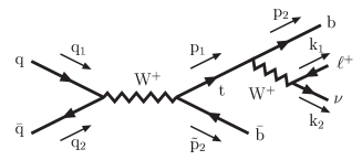
Figure 1.3: Feynman diagram contributing to single top production and decay process in the s-channel.

In Chapter 6 we show how the differential cross section corresponding to the process of Fig. (1.3) is calculated in a two step process using the narrow-width approximation with the top spin taken into account. That is, we first calculate the probability of producing tops with a given polarization and then we convolute it with the probability of decay summing over both polarizations. We argue how quantum interference effects can be minimized by the appropriate choice of spin basis. We present explicit expressions for the top spin basis that diagonalizes top density matrix both for the t- and s- channels. In the case of the s-channel we use this basis in our Monte Carlo integration and we check numerically how sensitive our results are to a change of spin-basis or even to disregarding top spin altogether This numerical study shows that the implementation of the correct spin basis is numerically important at the 4% level. Besides the top-spin issue, our simulations clearly show the crucial role of selecting specific kinematical configurations for the top decay products in order to achieve maximal sensitivity to $g_{R}$ both in magnitude and phase.

In the appendices of this thesis we have included technical material that complement the contents of the chapters and some calculations that can be a useful reference for those interested in some technical results. In particular we have included the complete calculation of all fermionic self-energies in an arbitrary $R_{\xi}$ gauges.

Chapter 2 The effective Lagrangian approach in the matter sector

The Standard Model of electroweak interactions has by now been impressively tested up to one part in a thousand level thanks to the formidable experimental work of LEP, SLC and other experiments in recent years. However, when it comes to the symmetry breaking mechanism clouds remain in this otherwise bright horizon and the mechanism giving masses to $W^{\pm}$, $Z,$ and fermions remains largely veiled.

The effective Lagrangian approach has already proven remarkably useful in setting very stringent bounds on some types of new physics taking as input basically the LEP [12] (and SLC [13]) experimental results. One writes the most general Lagrangian describing the interactions between the gauge sector and the Goldstone bosons appearing after the $SU(2)_{L}\times SU(2)_{R}\rightarrow SU(2)_{V}$ breaking . Since nothing is assumed for this breaking, the procedure is completely universal. The dependence on the specific model underlying the symmetry breaking is contained in the coefficients of higher dimensional operators. These kind of techniques —inherited from pion physics— have been already used to analyze contributions to the $S$, $T$ and $U$ parameters [41] and extract useful constraints on the models of symmetry breaking from them.

Our purpose in this chapter is to extend these techniques to the matter sector of the Standard Model. We shall write the leading non-universal operators, determine how their coefficients affect different physical observables and then determine their value in two very general families of models: those containing elementary scalars and those with dynamical symmetry breaking. Since the latter become non-perturbative at the $M_{Z}$ scale, effective Lagrangian techniques are called for anyway. In short, we would like to provide the theoretical tools required to test —at least in principle— whether the mechanism giving masses to quarks and fermions is the same as that which makes the intermediate vector bosons massive or not without having to get involved in the nitty-gritty details of particular models.

1 The effective Lagrangian approach

Let us start by briefly recalling the salient features of the effective Lagrangian analysis of the oblique corrections.

Including only those operators which are relevant for oblique corrections, the effective Lagrangian reads (see e.g. [37, 39] for the complete Lagrangian)

$$\mathcal{L}_{\mathrm{eff}}=\frac{v^{2}}{4}\mathrm{tr}D_{\mu}UD^{\mu}U^{\dagger}+a_{0}{g^{\prime}}^{2}\frac{v^{2}}{4}(\mathrm{tr}TD_{\mu}UU^{\dagger})^{2}+a_{1}gg^{\prime}\mathrm{tr}UB_{\mu\nu}U^{\dagger}W^{\mu\nu}-a_{8}\frac{g^{2}}{4}(\mathrm{tr}TW^{\mu\nu})^{2},$$ (2.1)

where $U=\exp(i\tau\cdot\chi/v)$ contains the 3 Goldstone bosons generated after the breaking of the global symmetry $SU(2)_{L}\times SU(2)_{R}\rightarrow SU(2)_{V}$. The covariant derivative is defined by

$$D_{\mu}U=\partial_{\mu}U+ig\frac{\tau}{2}\cdot W_{\mu}U-ig^{\prime}U\frac{\tau^{3}}{2}B_{\mu},.$$ (2.2)

$B_{\mu\nu}$ and $W^{\mu\nu}$ are the field-strength tensors corresponding to the right and left gauge groups, respectively

$$W_{\mu\nu}=\frac{\vec{\tau}}{2}\cdot\vec{W}_{\mu\nu},\qquad B_{\mu\nu}=\frac{\tau^{3}}{2}(\partial_{\mu}B_{\nu}-\partial_{\nu}B_{\mu}),$$ (2.3)

and $T=U\tau^{3}U^{\dagger}$. Only terms up to order $\mathcal{O}(p^{4})$ have been included. The reason is that dimensional counting arguments suppress, at presently accessible energies, higher dimensional terms, in the hypothesis that all undetected particles are much heavier than those included in the effective Lagrangian. While the first term on the r.h.s. of (2.1) is universal (in the unitary gauge it is just the mass term for the $W^{\pm}$ and $Z$ bosons), the coefficients $a_{0}$, $a_{1}$ and $a_{8}$ are non-universal. In other words, they depend on the specific mechanism responsible for the symmetry breaking. (Throughout this chapter the term ‘universal’ means ‘independent of the specific mechanism triggering $SU(2)_{L}\times SU(2)_{R}\rightarrow SU(2)_{V}$ breaking’.)

Most $Z$-physics observables relevant for electroweak physics can be parametrized in terms of vector and axial couplings $g_{V}$ and $g_{A}$ (see section 4). These are, in practice, flavor-dependent since they include vertex corrections which depend on the specific final state. Oblique corrections are however the same for all final states. The non-universal (but generation-independent) contributions to $g_{V}$ and $g_{A}$ coming from the effective Lagrangian (2.1) are

$$\bar{g}_{V} = a_{0}g^{\prime\,2}\left[\frac{\tau^{3}}{2}+2Q_{f}\left(2c_{W}^{2}-s_{W}^{2}\right)\right]+2a_{1}Q_{f}g^{2}s_{W}^{2}+2a_{8}Q_{f}g^{2}c_{W}^{2},$$ (2.4)

$$\bar{g}_{A} = a_{0}\frac{\tau^{3}}{2}g^{\prime\,2}.$$ (2.5)

They do depend on the specific underlying breaking mechanism through the values of the $a_{i}$. It should be noted that these coefficients depend logarithmically on some unknown scale. In the minimal Standard Model the characteristic scale is the Higgs boson mass, $M_{H}$. In other theories the scale $M_{H}$ will be replaced by some other scale $\Lambda$. A crucial prediction of chiral perturbation theory is that the dependence on these different scales is logarithmic and actually the same. It is thus possible to eliminate this dependence by building suitable combinations of $g_{V}$ and $g_{A}$ [38, 40] determined by the condition of absence of logs. Whether this line intersects or not the experimentally allowed region is a direct test of the nature of the symmetry breaking sector, independently of the precise value of Higgs mass (in the minimal Standard Model) or of the scale of new interactions (in other scenarios).

One could also try to extract information about the individual coefficients $a_{0}$, $a_{1}$ and $a_{8}$ themselves, and not only on the combinations cancelling the dependence on the unknown scale. This necessarily implies assuming a specific value for the scale $\Lambda$ and one should be aware that when considering these scale dependent quantities there are finite uncertainties of order $1/16\pi^{2}$ associated to the subtraction procedure —an unavoidable consequence of using an effective theory, that is often overlooked. (And recall that using an effective theory is almost mandatory in dynamical symmetry breaking models.) Only finite combinations of coefficients have a universal meaning. The subtraction scale uncertainty persists when trying to find estimates of the above coefficients via dispersion relations and the like [41].

In the previous analysis it is assumed that the hypothetical new physics contributions from vertex corrections are completely negligible. But is it so? The way to analyze such vertex corrections in a model-independent way is quite similar to the one outlined for the oblique corrections. We shall introduce in the next section the most general effective Lagrangian describing the matter sector. In this sector there is one universal operator (playing a role analogous to that of the first operator on the r.h.s. of (2.1) in the purely bosonic sector)

$$\mathcal{L}_{\mathrm{eff}}=-v\mathrm{\bar{f}}Uy_{f}R\mathrm{f}+h.c.,\qquad y_{f}=y\mathbf{1}+y_{3}\tau_{3}.$$ (2.6)

It is an operator of dimension 3. In the unitary gauge $U=1$, it is just the mass term for the matter fields. For instance if $\bar{q}_{L}$ is the doublet $(\bar{t},\bar{b})$

$$m_{t}=v(y+y_{3})=vy_{t},\qquad m_{b}=v(y-y_{3})=vy_{b}.$$ (2.7)

Non-universal operators carrying in their coefficients the information on the mechanism giving masses to leptons and quarks will be of dimension 4 and higher.

We shall later derive the values of the coefficients corresponding to operators in the effective Lagrangian of dimension 4 within the minimal Standard Model in the large $M_{H}$ limit and see how the effective Lagrangian provides a convenient way of tracing the Higgs mass dependence in physical observables. We shall later argue that non-decoupling effects should be the same in other theories involving elementary scalars, such as e.g. the two-Higgs doublet model, replacing $M_{H}$ by the appropriate mass.

Large non-decoupling effects appear in theories of dynamical symmetry breaking and thus they are likely to produce large contributions to the dimension 4 coefficients. If the scale characteristic of the extended interactions (i.e. those responsible of the fermion mass generation) is much larger than the scale characteristic of the electroweak breaking, it makes sense to parametrize the former, at least at low energies, via effective four-fermion operators. We shall assume here that this clear separation of scales does take place and only in this case are the present techniques really accurate. The appearance of pseudo Goldstone bosons (abundant in models of dynamical breaking) may thus jeopardize our conclusions, as they bring a relatively light scale into the game (typically even lighter than the Fermi scale). In fact, for the observables we consider their contribution is not too important, unless they are extremely light. For instance a pseudo-Goldstone boson of 100 GeV can be accommodated without much trouble, as we shall later see.

The four-fermion operators we have just alluded to can involve either four ordinary quarks or leptons (but we will see that dimensional counting suggests that their contribution will be irrelevant at present energies with the exception of those containing the top quark), or two new (heavy) fermions and two ordinary ones. This scenario is quite natural in several extended technicolor (ETC) or top condensate (TopC) models [42, 43], in which the underlying dynamics is characterized by a scale $M$. At scales $\mu<M$ the dynamics can be modelled by four-fermion operators (of either technifermions in ETC models, or ordinary fermions of the third family in TopC models). We perform a classification of these operators. We shall concentrate in the case where technifermions appear in ordinary representations of $SU(2)_{L}\times SU(3)_{c}$ (hypercharge can be arbitrary). The classification will then be exhaustive. We shall discuss other representations as well, although we shall consider custodially preserving operators only, and only those operators which are relevant for our purposes.

As a matter of principle we have tried not to make any assumptions regarding the actual way different generations are embedded in the extended interactions. In practice, when presenting our numerical plots and figures, we are assuming that the appropriate group-theoretical factors are similar for all three generations of physical fermions.

It has been our purpose in this chapter to be as general as possible, not advocating or trying to put forward any particular theory. Thus, the analysis may, hopefully, remain useful beyond the models we have just used to motivate the problem. We hope to convey to the reader our belief that a systematic approach based on four-fermion operators and the effective Lagrangian treatment can be very useful.

2 The matter sector

Appelquist, Bowick, Cohler and Hauser established some time ago a list of $d=4$ operators [44]. These are the operators of lowest dimensionality which are non-universal. In other words, their coefficients will contain information on whatever mechanism Nature has chosen to make quarks and leptons massive. Of course operators of dimensionality 5, 6 and so on will be generated at the same time. We shall turn to these later. We have reanalyzed all possible independent operators of $d=4$ (see the discussion in appendix B.1) and we find the following ones

$$\mathcal{L}_{L}^{1} = i\mathrm{\bar{f}}M_{L}^{1}\gamma^{\mu}U\left(D_{\mu}U\right)^{\dagger}L\mathrm{f}+h.c.,$$ (2.8)

$$\mathcal{L}_{L}^{2} = i\mathrm{\bar{f}}M_{L}^{2}\gamma^{\mu}\left(D_{\mu}U\right)\tau^{3}U^{\dagger}L\mathrm{f}+h.c.,$$ (2.9)

$$\mathcal{L}_{L}^{3} = i\mathrm{\bar{f}}M_{L}^{3}\gamma^{\mu}U\tau^{3}U^{\dagger}\left(D_{\mu}U\right)\tau^{3}U^{\dagger}L\mathrm{f}+h.c.,$$ (2.10)

$$\mathcal{L}_{L}^{4} = i\mathrm{\bar{f}}M_{L}^{4}\gamma^{\mu}U\tau^{3}U^{\dagger}D_{\mu}^{L}L\mathrm{f}+h.c.,$$ (2.11)

$$\mathcal{L}_{R}^{1} = i\mathrm{\bar{f}}M_{R}^{1}\gamma^{\mu}U^{\dagger}\left(D_{\mu}U\right)R\mathrm{f}+h.c.,$$ (2.12)

$$\mathcal{L}_{R}^{2} = i\mathrm{\bar{f}}M_{R}^{2}\gamma^{\mu}\tau^{3}U^{\dagger}\left(D_{\mu}U\right)R\mathrm{f}+h.c.,$$ (2.13)

$$\mathcal{L}_{R}^{3} = i\mathrm{\bar{f}}M_{R}^{3}\gamma^{\mu}\tau^{3}U^{\dagger}\left(D_{\mu}U\right)\tau^{3}R\mathrm{f}+h.c.,$$ (2.14)

$$\mathcal{L}_{R}^{\prime} = i\mathrm{\bar{f}}M_{R}^{\prime}\tau^{3}\gamma^{\mu}D_{\mu}^{L}R\mathrm{f}+h.c..$$ (2.15)

Each operator is accompanied by a coefficient $M_{L,R}^{i}$. In this chapter we will not consider mixing and therefore these coefficient are pure numbers. In Chapter 3 mixing is considered and therefore we will allow the $M_{L,R}^{i}$ to have family indices. Thus, up to $\mathcal{O}(p^{4})$, our effective Lagrangian is

$$\mathcal{L}_{\mathrm{eff}}=\mathcal{L}_{R}^{\prime}+\sum_{i=1}^{4}\mathcal{L}_{L}^{i}+\sum_{i=1}^{3}\mathcal{L}_{R}^{i}.$$ (2.16)

In the above, $D_{\mu}U$ is defined in (2.2) whereas

$$D_{\mu}^{L}f_{L} = \left[\partial_{\mu}+ig\frac{\tau}{2}\cdot W_{\mu}+ig^{\prime}\left(Q-\frac{\tau^{3}}{2}\right)B_{\mu}+ig_{s}\frac{\lambda}{2}\cdot G_{\mu}\right]f_{L},$$

$$D_{\mu}^{R}f_{R} = \left[\partial_{\mu}+ig^{\prime}QB_{\mu}+ig_{s}\frac{\lambda}{2}\cdot G_{\mu}\right]f_{R},$$

where $Q$ is the electric charge given by

$$Q=\frac{\tau^{3}}{2}+z,$$

with $z=1/6$ for quarks and $z=-1/2$ for leptons and therefore with the hypercharge given by

$$Y=\left\{\begin{tabular}[]{ll}$z$&$\mathrm{for\ lefts.}$\\ $\frac{\tau^{3}}{2}+z$&$\mathrm{for\ rights.}$\end{tabular}\right.$$

This list differs from the one in [44] by the presence of the last operator (2.15). It will turn out, however, that $M_{R}^{\prime}$ does not contribute to any observable. All these operators are invariant under local $SU(2)_{L}\times U(1)_{Y}$ transformations.

This list includes both the custodially preserving operators $\mathcal{L}_{L}^{1}$ and $\mathcal{L}_{R}^{1}$ and the rest of operators that are custodially breaking ones. In the purely bosonic part of the effective Lagrangian (2.1), the first (universal) operator and the one accompanying $a_{1}$ are custodially preserving, while those going with $a_{0}$ and $a_{8}$ are custodially breaking. E.g., $a_{0}$ parametrizes the contribution of the new physics to the $\Delta\rho$ parameter. If the underlying physics is custodially preserving only $M_{L,R}^{1}$ will get non-vanishing contributions.

The operator $\mathcal{L}_{L}^{4}$ deserves some comments. By using the equations of motion it can be reduced to the mass term (2.6)

$$vM_{L}^{4}\mathrm{\bar{f}}U\tau^{3}y_{f}R\mathrm{f}+h.c.,$$

However this procedure is, generally speaking, only justified if the matter fields appear only as external legs. For the time being we shall keep $\mathcal{L}_{L}^{4}$ as an independent operator and in the next section we shall determine its value in the minimal Standard Model after integrating out a heavy Higgs. We shall see that, after imposing that physical on-shell fields have unit residue, $M_{L}^{4}$ does drop from all physical predictions.

What is the expected size of the $M_{L,R}^{i}$ coefficients in the minimal Standard Model? This question is easily answered if we take a look at the diagrams that have to be computed to integrate out the Higgs field (Fig. (2.2)). Notice that the calculation is carried out in the non-linear variables $U$, hence the appearance of the unfamiliar diagram e). Diagram d) is actually of order $1/M_{H}^{2}$, which guarantees the gauge independence of the effective Lagrangian coefficients. The diagrams are obviously proportional to $y^{2}$, $y$ being a Yukawa coupling, and also to $1/16\pi^{2}$, since they originate from a one-loop calculation. Finally, the screening theorem shows that they may depend on the Higgs mass only logarithmically, therefore

$$M_{L,R}^{i\left(\mathrm{SM}\right)}\sim{\frac{y^{2}}{{16\pi^{2}}}}\log{\frac{M_{H}^{2}}{M_{Z}^{2}}}.$$ (2.17)

These dimensional considerations show that the vertex corrections are only sizeable for third generation quarks.

In models of dynamical symmetry breaking, such as TC or ETC, we shall have new contributions to the $M_{L,R}^{i}$ from the new physics (which we shall later parametrize with four-fermion operators). We have several new scales at our disposal. One is $M$, the mass normalizing dimension six four-fermion operators. The other can be either $m_{b}$ (negligible, since $M$ is large), $m_{t}$, or the dynamically generated mass of the techniquarks $m_{Q}$ (typically of order $\Lambda_{TC}$, the scale associated to the interactions triggering the breaking of the electroweak group). Thus we can get a contribution of order

$$M_{L,R}^{i\left(\mathrm{Q}\right)}\sim\frac{1}{16\pi^{2}}\frac{m_{Q}^{2}}{M^{2}}\log\frac{m_{Q}^{2}}{M^{2}}.$$ (2.18)

While $m_{Q}$ is, at least naively, expected to be $\simeq\Lambda_{TC}$ and therefore similar for all flavors, there should be a hierarchy for $M$. As will be discussed in the following sections, the scale $M$ which is relevant for the mass generation (encoded in the only dimension 3 operator in the effective Lagrangian), via techniquark condensation and ETC interaction exchange (Fig. (2.1)), is the one normalizing chirality flipping operators. On the contrary, the scale normalizing dimension 4 operators in the effective theory is the one that normalizes chirality preserving operators. Both scales need not be exactly the same, and one may envisage a situation with relatively light scalars present where the former can be much lower. However, it is natural to expect that $M$ should at any rate be smallest for the third generation. Consequently the contribution to the $M_{L,R}^{i}$’s from the third generation should be largest.

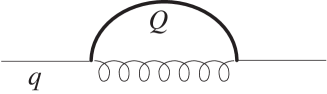
Figure 2.1: Mechanism generating quark masses through the exchange of a ETC particle.

We should also discuss dimension 5, 6, etc. operators and why we need not include them in our analysis. Let us write some operators of dimension 5:

$$\mathrm{\bar{f}}\hat{W}UR\mathrm{f}+h.c.,$$

$$\mathrm{\bar{f}}U\hat{B}R\mathrm{f}+h.c.,$$

$$\mathrm{\bar{f}}\sigma^{\mu\nu}\left(D_{\mu}\left(D_{\nu}U\right)\right)^{\dagger}R\mathrm{f}+h.c.,$$

$$\mathrm{\bar{f}}\sigma^{\mu\nu}\left(D_{\mu}U\right)^{\dagger}D_{\nu}R\mathrm{f}+h.c.,$$

$$\mathrm{\bar{f}}UD^{2}R\mathrm{f}+h.c.,$$

where we use the notation $\hat{W}\equiv ig\sigma^{\mu\nu}W_{\mu\nu}$, $\hat{B}\equiv ig^{\prime}\sigma^{\mu\nu}B_{\mu\nu}$. These are a few of a long list of about 25 operators, and this including only the ones contributing to the $ffZ$ vertex. All these operators are however chirality flipping and thus their contribution to the amplitude must be suppressed by one additional power of the fermion masses. This makes their study unnecessary at the present level of precision. Similar considerations apply to operators of dimensionality 6 or higher.

3 The effective theory of the Standard Model

In this section we shall obtain the values of the coefficients $M_{L,R}^{i}$ in the minimal Standard Model. The appropriate effective coefficients for the oblique corrections $a_{i}$ have been obtained previously by several authors [38, 40, 46]. Their values are

$$a_{0} = \frac{1}{16\pi^{2}}\frac{3}{8}\left(\frac{1}{\hat{\epsilon}}-\log\frac{M_{H}^{2}}{\mu^{2}}+\frac{5}{6}\right),$$ (2.19)

$$a_{1} = \frac{1}{16\pi^{2}}\frac{1}{12}\left(\frac{1}{\hat{\epsilon}}-\log\frac{M_{H}^{2}}{\mu^{2}}+\frac{5}{6}\right),$$ (2.20)

$$a_{8} = 0.$$ (2.21)

where $1/\hat{\epsilon}\equiv 1/\epsilon-\gamma_{E}+\log 4\pi$. We use dimensional regularization with a space-time dimension $4-2\epsilon$.

We begin by writing the Standard Model in terms of the non-linear variables $U$. The matrix

$$\mathcal{M}=\sqrt{2}(\tilde{\Phi},\Phi),$$ (2.22)

constructed with the Higgs doublet, $\Phi$ and its conjugate, $\tilde{\Phi}\equiv i\tau^{2}\Phi^{\ast}$, is rewritten in the form

$$\mathcal{M}=(v+\rho)U,\qquad U^{-1}=U^{\dagger},$$ (2.23)

where $\rho$ describe the ‘radial’ excitations around the v.e.v. $v$. Integrating out the field $\rho$ produces an effective Lagrangian of the form (2.1) with the values of the $a_{i}$ given above (as well as some other pieces not shown there). This functional integration also generates the vertex corrections (2.16).

We shall determine the $M_{L,R}^{i}$ by demanding that the renormalized one-particle irreducible Green functions (1PI), $\hat{\Gamma}$, are the same (up to some power in the external momenta and mass expansion) in both, the minimal Standard Model and the effective Lagrangian. In other words, we require that

$$\Delta\hat{\Gamma}=0,$$ (2.24)

where throughout this section

$$\Delta\Gamma\equiv\Gamma_{\mathrm{SM}}-\Gamma_{\mathrm{eff}},$$ (2.25)

and the hat denotes renormalized quantities. This procedure is known as matching. It goes without saying that in doing so the same renormalization scheme must be used. The on-shell scheme is particularly well suited to perform the matching and will be used throughout this work.

One only needs to worry about SM diagrams that are not present in the effective theory; namely, those containing the Higgs. The rest of the diagrams give exactly the same result, thus dropping from the matching. In contrast, the diagrams containing a Higgs propagator are described by local terms (such as $\mathcal{L}_{L}^{1}$ through $\mathcal{L}_{L}^{4}$) in the effective theory, they involve the coefficients $M_{L,R}^{i}$, and give rise to the Feynman rules collected in appendix B.2.

Let us first consider the fermion self-energies. There is only one 1PI diagram with a Higgs propagator (see Fig. (2.2)).

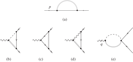
Figure 2.2: The diagrams relevant for the matching of the fermion self-energies and vertices (counterterm diagrams are not included). Double lines represent the Higgs, dashed lines the Goldstone bosons, and wiggly lines the gauge bosons.

A straightforward calculation gives

$$\Sigma_{\mathrm{SM}}^{f}=-{\frac{y_{f}^{2}}{16\pi^{2}}}\left\{\not{p}\left[{\frac{1}{2}}\frac{1}{\hat{\epsilon}}-{\frac{1}{2}}\log{\frac{M_{H}^{2}}{\mu^{2}}}+{\frac{1}{4}}\right]+m_{f}\left[\frac{1}{\hat{\epsilon}}-\log{\frac{M_{H}^{2}}{\mu^{2}}}+1\right]\right\}.$$ (2.26)

$\Delta\Sigma^{f}$ can be computed by subtracting Eqs. (B.13) and (B.14) from Eq. (2.26).

Next, we have to renormalize the fermion self-energies. We introduce the following notation

$$\Delta Z\equiv Z_{\mathrm{SM}}-Z_{\mathrm{eff}}=\delta Z_{\mathrm{SM}}-\delta Z_{\mathrm{eff}},$$ (2.27)

where $Z_{\mathrm{SM}}$ ($Z_{\mathrm{eff}}$) stands for any renormalization constant of the SM (effective theory). To compute $\Delta\hat{\Sigma}^{f}$, we simply add to $\Delta\Sigma^{f}$ the counterterm diagram (B.47) with the replacements $\delta Z_{V,A}^{f}\rightarrow\Delta Z_{V,A}^{f}$ and $\delta m_{f}\rightarrow\Delta m_{f}$. This, of course, amounts to Eqs. (B.54), (B.55) and (B.56) with the same replacements. From Eqs. (B.57), (B.58) and (B.59) (which also hold for $\Delta Z$, $\Delta m$ and $\Delta\Sigma$) one can express $\Delta Z_{V,A}^{f}$ and $\Delta m_{f}/m_{f}$ in terms of the bare fermion self-energies and finally obtain $\Delta\hat{\Sigma}^{f}$. The result is

$$\Delta\hat{\Sigma}_{A,V,S}^{d} = 0,$$ (2.28)

$$\Delta\hat{\Sigma}_{A}^{u} = 0,$$ (2.29)

$$\Delta\hat{\Sigma}_{V,S}^{u} = 4M_{L}^{4}-{\frac{1}{16\pi^{2}}}{\frac{y_{u}^{2}-y_{d}^{2}}{2}}\left[\frac{1}{\hat{\epsilon}}-\log{\frac{M_{H}^{2}}{\mu^{2}}}+{\frac{1}{2}}\right].$$ (2.30)

We see from Eq. (2.30) that the matching conditions, $\Delta\hat{\Sigma}_{V,S}^{u}=0$, imply

$$M_{L}^{4}={\frac{1}{16\pi^{2}}}{\frac{y_{u}^{2}-y_{d}^{2}}{8}}\left[\frac{1}{\hat{\epsilon}}-\log{\frac{M_{H}^{2}}{\mu^{2}}}+{\frac{1}{2}}\right].$$ (2.31)

The other matchings are satisfied automatically and do not give any information.

Let us consider the vertex $ffZ$. The relevant diagrams are shown in Fig. (2.2) (diagrams b–e). We shall only collect the contributions proportional to $\gamma_{\mu}$ and $\gamma_{\mu}\gamma_{5}$. Remembering

$$s_{W} \equiv \sin\theta_{W}\equiv\frac{g^{\prime}}{\sqrt{g^{2}+g^{\prime\,2}}},\qquad c_{W}\equiv\cos\theta_{W}\equiv\frac{g}{\sqrt{g^{2}+g^{\prime\,2}}},$$

$$e \equiv gs_{W}=g^{\prime}c_{W},\qquad W_{\mu}^{3}=s_{W}A_{\mu}+c_{W}Z_{\mu},\qquad B_{\mu}=c_{W}A_{\mu}-s_{W}Z_{\mu},$$ (2.32)

and Eq. (B.52) the result is

$$\Gamma_{\mu}^{ffZ}={\frac{-1}{16\pi^{2}}}{\frac{y_{f}^{2}}{2}}\gamma_{\mu}\left\{v_{f}\left(\frac{1}{\hat{\epsilon}}-\log{\frac{M_{H}^{2}}{\mu^{2}}}+{\frac{1}{2}}\right)-3a_{f}\,\gamma_{5}\left(\frac{1}{\hat{\epsilon}}-\log{\frac{M_{H}^{2}}{\mu^{2}}}+{\frac{11}{6}}\right)\right\}.$$ (2.33)

By subtracting the diagrams (B.8) and (B.9) from $\Gamma_{\mu}^{ffZ}$ one gets $\Delta\Gamma_{\mu}^{ffZ}$. Renormalization requires that we add the counterterm diagram (B.48) where, again, $\delta Z\rightarrow\Delta Z$. One can check that both $\Delta Z_{1}^{Z}-\Delta Z_{2}^{Z}$ and $\Delta Z_{1}^{Z\gamma}-\Delta Z_{2}^{Z\gamma}$ are proportional to $\Delta\Sigma_{Z\gamma}(0)$, which turns out to be zero. Hence the only relevant renormalization constants are $\Delta Z_{V}^{f}$ and $\Delta Z_{A}^{f}$. These renormalization constant have already been determined. One obtains for $\Delta\hat{\Gamma}_{\mu}^{ffZ}$ the result

$$\Delta\hat{\Gamma}_{\mu}^{ddZ} = {\frac{-e}{2s_{W}c_{W}}}\gamma_{\mu}\left\{\left[M_{L}^{1}-M_{L}^{3}-M_{R}^{1}-M_{R}^{3}+M_{L}^{2}+M_{R}^{2}\right]\right.$$

$$- \left.\gamma_{5}\left[{\frac{1}{16\pi^{2}}}{\frac{y_{d}^{2}}{2}}\left(\frac{1}{\hat{\epsilon}}-\log{\frac{M_{H}^{2}}{\mu^{2}}}+{\frac{5}{2}}\right)+M_{L}^{1}-M_{L}^{3}+M_{R}^{1}+M_{R}^{3}+M_{L}^{2}-M_{R}^{2}\right]\right\}$$

$$\Delta\hat{\Gamma}_{\mu}^{uuZ} = {\frac{e}{2s_{W}c_{W}}}\gamma_{\mu}\left\{\left[M_{L}^{1}-M_{L}^{3}-M_{R}^{1}-M_{R}^{3}-M_{L}^{2}-M_{R}^{2}\right]\right.$$

$$- \left.\gamma_{5}\left[{\frac{1}{16\pi^{2}}}{\frac{y_{u}^{2}}{2}}\left(\frac{1}{\hat{\epsilon}}-\log{\frac{M_{H}^{2}}{\mu^{2}}}+{\frac{5}{2}}\right)+M_{L}^{1}-M_{L}^{3}+M_{R}^{1}+M_{R}^{3}-M_{L}^{2}+M_{R}^{2}\right]\right\},$$

where use has been made of Eq. (2.31). The matching condition, $\Delta\hat{\Gamma}_{\mu}^{ffZ}=0$ implies

$$M_{L}^{1}-M_{L}^{3} = -{\frac{1}{16\pi^{2}}}{\frac{y_{u}^{2}+y_{d}^{2}}{8}}\left(\frac{1}{\hat{\epsilon}}-\log{\frac{M_{H}^{2}}{\mu^{2}}}+{\frac{5}{2}}\right),$$ (2.34)

$$M_{R}^{1}+M_{R}^{3} = -{\frac{1}{16\pi^{2}}}{\frac{y_{u}^{2}+y_{d}^{2}}{8}}\left(\frac{1}{\hat{\epsilon}}-\log{\frac{M_{H}^{2}}{\mu^{2}}}+{\frac{5}{2}}\right),$$ (2.35)

$$M_{L}^{2} = {\frac{1}{16\pi^{2}}}{\frac{y_{u}^{2}-y_{d}^{2}}{8}}\left(\frac{1}{\hat{\epsilon}}-\log{\frac{M_{H}^{2}}{\mu^{2}}}+{\frac{5}{2}}\right),$$ (2.36)

$$M_{R}^{2} = -{\frac{1}{16\pi^{2}}}{\frac{y_{u}^{2}-y_{d}^{2}}{8}}\left(\frac{1}{\hat{\epsilon}}-\log{\frac{M_{H}^{2}}{\mu^{2}}}+{\frac{5}{2}}\right).$$ (2.37)

To determine completely the $M_{L,R}^{i}$ coefficients we need to consider the vertex $udW$. The relevant diagrams are analogous to those of Fig. 2.2. A straightforward calculation gives

$$\Delta\hat{\Gamma}_{\mu}^{udW} = {\frac{e}{4\sqrt{2}s_{W}}}\;\gamma_{\mu}\left\{\left[{\frac{y_{u}y_{d}}{16\pi^{2}}}\left(\frac{1}{\hat{\epsilon}}-\log{\frac{M_{H}^{2}}{\mu^{2}}}+{\frac{5}{2}}\right)+4\left(M_{R}^{1}-M_{R}^{3}\right)\right](1+\gamma_{5})\right.$$

$$\left.-\left[{\frac{y_{u}^{2}+y_{d}^{2}}{16\pi^{2}}}\frac{1}{2}\left(\frac{1}{\hat{\epsilon}}-\log{\frac{M_{H}^{2}}{\mu^{2}}}+{\frac{5}{2}}\right)+4\left(M_{L}^{1}+M_{L}^{3}\right)\right](1-\gamma_{5})\right\}.$$

The matching condition $\Delta\hat{\Gamma}_{\mu}^{udW}=0$ amounts to the following set of equations

$$M_{R}^{1}-M_{R}^{3} = -{\frac{1}{16\pi^{2}}}{\frac{y_{u}y_{d}}{4}}\left(\frac{1}{\hat{\epsilon}}-\log{\frac{M_{H}^{2}}{\mu^{2}}}+{\frac{5}{2}}\right),$$

$$M_{L}^{1}+M_{L}^{3} = -{\frac{1}{16\pi^{2}}}{\frac{y_{u}^{2}+y_{d}^{2}}{8}}\left(\frac{1}{\hat{\epsilon}}-\log{\frac{M_{H}^{2}}{\mu^{2}}}+{\frac{5}{2}}\right),$$

Combining these equations with Eqs. (2.34, 2.35) we finally get

$$M_{L}^{1} = -{\frac{1}{16\pi^{2}}}{\frac{y_{u}^{2}+y_{d}^{2}}{8}}\left(\frac{1}{\hat{\epsilon}}-\log{\frac{M_{H}^{2}}{\mu^{2}}}+{\frac{5}{2}}\right),$$ (2.38)

$$M_{R}^{1} = -{\frac{(y_{u}+y_{d})^{2}}{\left(16\pi\right)^{2}}}\left(\frac{1}{\hat{\epsilon}}-\log{\frac{M_{H}^{2}}{\mu^{2}}}+{\frac{5}{2}}\right),$$ (2.39)

$$M_{L}^{3} = 0,$$ (2.40)

$$M_{R}^{3} = -{\frac{(y_{u}-y_{d})^{2}}{\left(16\pi\right)^{2}}}\left(\frac{1}{\hat{\epsilon}}-\log{\frac{M_{H}^{2}}{\mu^{2}}}+{\frac{5}{2}}\right),$$ (2.41)

This, along with Eqs. (2.36, 2.37) and Eq. (2.31), is our final answer. These results coincide, where the comparison is possible, with those obtained in [47] by functional methods. It is interesting to note that it has not been necessary to consider the matching of the vertex $ff\gamma$.

We shall show explicitly that $M_{L}^{4}$ drops from the $S$ matrix element corresponding to $Z\rightarrow f\bar{f}$. It is well known that the renormalized $u$-fermion propagator has residue $1+\delta_{res}$, where $\delta_{res}$ is given in Eq. (B.60) of appendix B.4. Therefore, in order to evaluate $S$-matrix elements involving external $u$ lines at one-loop, one has to multiply the corresponding amputated Green functions by a factor $1+n\,\delta_{res}/2$, where $n$ is the number on external $u$-lines (in the case under consideration $n=2$). One can check that when this factor is taken into account, the $M_{L}^{4}$ appearing in the renormalized S-matrix vertex are cancelled.

We notice that $M_{L}^{1}$ and $M_{R}^{1}$ indeed correspond to custodially preserving operators, while $M_{L,R}^{2}$ and $M_{L,R}^{3}$ do not. All these coefficients (just as $a_{0}$, $a_{1}$ and $a_{8}$) are ultraviolet divergent (with the exception of $M_{L}^{3}$). This is so because the Higgs particle is an essential ingredient to guarantee the renormalizability of the Standard Model. Once this is removed, the usual renormalization process (e.g. the on-shell scheme) is not enough to render all “renormalized” Green functions finite. This is why the bare coefficients of the effective Lagrangian (which contribute to the renormalized Green functions either directly or via counterterms) have to be proportional to $1/\epsilon$ to cancel the new divergences. The coefficients of the effective Lagrangian are manifestly gauge invariant.

What is the value of these coefficients in other theories with elementary scalars and Higgs-like mechanism? This issue has been discussed in some detail in [48] in the context of the two-Higgs doublet model, but it can actually be extended to supersymmetric theories (provided of course scalars other than the $CP$-even Higgs can be made heavy enough, see e.g. [49]). It was argued there that non-decoupling effects are exactly the same as in the minimal Standard Model, including the constant non-logarithmic piece. Since the $M_{L,R}^{i}$ coefficients contain all the non-decoupling effects associated to the Higgs particle at the first non-trivial order in the momentum or mass expansion, the low energy effective theory will be exactly the same.

4 Z decay observables

The decay width of $Z\rightarrow f\bar{f}$ is described by

$$\Gamma_{f}\equiv\Gamma\left(Z\rightarrow f\bar{f}\right)=4n_{c}\Gamma_{0}\left[\left(g_{V}^{f}\right)^{2}R_{V}^{f}+\left(g_{A}^{f}\right)^{2}R_{A}^{f}\right],$$ (2.42)

where $g_{V}^{f}$ and $g_{A}^{f}$ are the effective electroweak couplings as defined in [50] and $n_{c}$ is the number of colors of fermion $f$. The radiation factors $R_{V}^{f}$ and $R_{A}^{f}$ describe the final state QED and QCD interactions [51]. For a charged lepton we have

$$R_{V}^{l} = 1+\frac{3\bar{\alpha}}{4\pi}+\mathcal{O}\left(\bar{\alpha}^{2},\left(\frac{m_{l}}{M_{Z}}\right)^{4}\right),$$

$$R_{A}^{l} = 1+\frac{3\bar{\alpha}}{4\pi}-6\left(\frac{m_{l}}{M_{Z}}\right)^{2}+\mathcal{O}\left(\bar{\alpha}^{2},\left(\frac{m_{l}}{M_{Z}}\right)^{4}\right),$$

where $\bar{\alpha}$ is the electromagnetic coupling constant at the scale $M_{Z}$ and $m_{l}$ is the final state lepton mass

The tree-level width $\Gamma_{0}$ is given by

$$\Gamma_{0}=\frac{G_{\mu}M_{Z}^{3}}{24\sqrt{2}\pi}.$$ (2.43)

If we define

$$\rho_{f} \equiv 4\left(g_{A}^{f}\right)^{2},$$ (2.44)

$$\bar{s}_{W}^{2} \equiv \frac{\tau^{3}}{4Q_{f}}\left(1-\frac{g_{V}^{f}}{g_{A}^{f}}\right),$$ (2.45)

we can write

$$\Gamma_{f}=n_{c}\Gamma_{0}\rho_{f}\left[4\left(\frac{\tau^{3}}{2}-2Q_{f}\bar{s}_{W}^{2}\right)^{2}R_{V}^{f}+R_{A}^{f}\right].$$ (2.46)

Other quantities which are often used are $\Delta\rho_{f}$, defined through

$$\rho_{f}\equiv\frac{1}{1-\Delta\rho_{f}},$$ (2.47)

the forward-backward asymmetry $A_{FB}^{f}$

$$A_{FB}^{f}=\frac{3}{4}A^{e}A^{f},$$ (2.48)

and $R_{b}$

$$R_{b}=\frac{\Gamma_{b}}{\Gamma_{h}},$$ (2.49)

where

$$A^{f}\equiv\frac{2g_{V}^{f}g_{A}^{f}}{\left(g_{A}^{f}\right)^{2}+\left(g_{V}^{f}\right)^{2}},$$

and $\Gamma_{b}$, $\Gamma_{h}$ are the b-partial width and total hadronic width, respectively (each of them, in turn, can be expressed in terms of the appropriate effective couplings). As we see, nearly all of $Z$ physics can be described in terms of $g_{A}^{f}$ and $g_{V}^{f}$. The box contributions to the process $e^{+}e^{-}\rightarrow f\bar{f}$ are not included in the analysis because they are negligible and they cannot be incorporated as contributions to effective electroweak neutral current couplings anyway.

We shall generically denote these effective couplings by $g^{f}$. If we express the value they take in the Standard Model by $g^{f\left(\mathrm{SM}\right)}$, we can write a perturbative expansion for them in the following way

$$g^{f\left(\mathrm{SM}\right)}=g^{f\left(0\right)}+g^{f\left(2\right)}+\bar{g}^{f}(a_{i}^{\mathrm{(SM)}})+\hat{g}^{f}(M_{L,R}^{i\mathrm{(SM)}}),$$ (2.50)

where $g^{f\left(0\right)}$ are the tree-level expressions for these form factors, $g^{f\left(2\right)}$ are the one-loop contributions which do not contain any Higgs particle as internal line in the Feynman graphs. In the effective Lagrangian language they are generated by the quantum corrections computed by operators such as (2.6) or the first operator on the r.h.s. of (2.1). On the other hand, the Feynman diagrams containing the Higgs particle contribute to $g^{f\left(\mathrm{SM}\right)}$ in a twofold way. One is via the $\mathcal{O}(p^{2})$ and $\mathcal{O}(p^{4})$ Longhitano effective operators (2.1) which depend on the $a_{i}$ coefficients, which are Higgs-mass dependent, and thus give a Higgs-dependent oblique correction to $g^{f\left(\mathrm{SM}\right)}$, which is denoted by $\bar{g}^{f}$. The other one is via genuine vertex corrections which depend on the $M_{L,R}^{i}$. This contribution is denoted by $\hat{g}^{f}$.

The tree-level value for the form factors are

$$g_{V}^{f\left(0\right)}=\frac{\tau^{3}}{2}-2s_{W}^{2}Q_{f},\qquad g_{A}^{f\left(0\right)}=\frac{\tau^{3}}{2}.$$ (2.51)

In a theory X, different from the minimal Standard Model, the effective form factors will take values $g^{f\left(\mathrm{X}\right)}$, where

$$g^{f\left(\mathrm{X}\right)}=g^{f\left(0\right)}+g^{f\left(2\right)}+\bar{g}^{f}(a_{i}^{\mathrm{(X)}})+\hat{g}^{f}(M_{L,R}^{i\mathrm{(X)}}),$$ (2.52)

and the $a_{i}^{\mathrm{(X)}}$ and $M_{L,R}^{i\mathrm{(X)}}$ are effective coefficients corresponding to theory X.

Within one-loop accuracy in the symmetry breaking sector (but with arbitrary precision elsewhere), $\bar{g}^{f}$ and $\hat{g}^{f}$ are linear functions of their arguments and thus we have

$$g^{f\left(\mathrm{X}\right)}=g^{f\left(\mathrm{SM}\right)}+\bar{g}^{f}(a_{i}^{\mathrm{(X)}}-a_{i}^{\mathrm{(SM)}})+\hat{g}^{f}(M_{L,R}^{i\mathrm{(X)}}-M_{L,R}^{i\mathrm{(SM)}}).$$ (2.53)

The expression for $\bar{g}^{f}$ in terms of $a_{i}$ was already given in Eqs. (2.4) and (2.5). On the other hand from appendix B.2 we learn that

$$\hat{g}_{V}^{f}\left(M_{L,R}^{i}\right) = M_{L}^{2}+M_{R}^{2}-\tau^{3}\left(M_{L}^{1}-M_{L}^{3}-M_{R}^{1}-M_{R}^{3}\right),$$

$$\hat{g}_{A}^{f}\left(M_{L,R}^{i}\right) = M_{L}^{2}-M_{R}^{2}-\tau^{3}\left(M_{L}^{1}-M_{L}^{3}+M_{R}^{1}+M_{R}^{3}\right),$$

In the minimal Standard Model all the Higgs dependence at the one loop level (which is the level of accuracy assumed here) is logarithmic and is contained in the $a_{i}$ and $M_{L,R}^{i}$ coefficients. Therefore one can easily construct linear combinations of observables where the leading Higgs dependence cancels. These combinations allow for a test of the minimal Standard Model independent of the actual value of the Higgs mass.

Let us now review the comparison with current electroweak data for theories with dynamical symmetry breaking. Some confusion seem to exist on this point so let us try to analyze this issue critically.

A first difficulty arises from the fact that at the $M_{Z}$ scale perturbation theory is not valid in theories with dynamical breaking and the contribution from the symmetry breaking sector must be estimated in the framework of the effective theory, which is non-linear and non-renormalizable. Observables will depend on some subtraction scale. (Estimates based on dispersion relations and resonance saturation amount, in practice, to the same, provided that due attention is paid to the scale dependence introduced by the subtraction in the dispersion relation.)

A somewhat related problem is that, when making use of the variables $S,T$ and $U$ [41], or $\epsilon_{1},\epsilon_{2}$ and $\epsilon_{3}$ [52], one often sees in the literature bounds on possible “new physics” in the symmetry breaking sector without actually removing the contribution from the Standard Model Higgs that the “new physics” is supposed to replace (this is not the case e.g. in [41] where this issue is discussed with some care). Unless the contribution from the “new physics” is enormous, this is a flagrant case of double counting, but it is easy to understand why this mistake is made: removing the Higgs makes the Standard Model non-renormalizable and the observables of the Standard Model without the Higgs depend on some arbitrary subtraction scale.

In fact the two sources of arbitrary subtraction scales (the one originating from the removal of the Higgs and the one from the effective action treatment) are one an the same and the problem can be dealt with the help of the coefficients of higher dimensional operators in the effective theory (i.e. the $a_{i}$ and $M_{L,R}^{i}$). The dependence on the unknown subtraction scale is absorbed in the coefficients of higher dimensional operators and traded by the scale of the “new physics”. Combinations of observables can be built where this scale (and the associated renormalization ambiguities) drops. These combinations allow for a test of the “new physics” independently of the actual value of its characteristic scale. In fact they are the same combinations of observables where the Higgs dependence drops in the minimal Standard Model.

A third difficulty in making a fair comparison of models of dynamical symmetry breaking with experiment lies in the vertex corrections. If we analyze the lepton effective couplings $g_{A}^{l}$ and $g_{V}^{l}$, the minimal Standard Model predicts very small vertex corrections arising from the symmetry breaking sector anyway and it is consistent to ignore them and concentrate in the oblique corrections. However, this is not the situation in dynamical symmetry breaking models. We will see in the next sections that for the second and third generation vertex corrections can be sizeable. Thus if we want to compare experiment to oblique corrections in models of dynamical breaking we have to concentrate on electron couplings only.

Figure 2.3: The $1-\sigma$ experimental region in the $g_{A}^{e}-g_{V}^{e}$ plane. The Standard Model predictions as a function of $m_{t}$ ($170.6\leq m_{t}\leq 180.6$ GeV) and $M_{H}$ ($70\leq M_{H}\leq 1000$ GeV) are shown (the middle line corresponds to the central value $m_{t}=175.6$ GeV). The predictions of a QCD-lke technicolor theory with $n_{TC}n_{D}=8$ and degenerate technifermion masses are shown as straight lines (only oblique corrections are included). One moves along the straight lines by changing the scale $\Lambda$. The three lines correspond to the extreme and central values for $m_{t}$. Recall that the precise location anywhere on the straight lines (which definitely do intersect the $1-\sigma$ region) depends on the renormalization procedure and thus is not predictable within the non-renormalizable effective theory. In addition the technicolor prediction should be considered accurate only at the 15% level due to the theoretical uncertainties discussed in the text (this error is at any rate smaller than the one associated to the uncertainty in $\Lambda$). Notice that the oblique corrections, in the case of degenerate masses, are independent of the value of the technifermion mass. Assuming universality of the vertex corrections reduces the error bars by about a factor one-half and leaves technicolor predictions outside the $1-\sigma$ region.

In Fig. 2.3 we see the prediction of the minimal Standard Model for $170.6<m_{t}<180.6$ GeV and $70<M_{H}<1000$ GeV including the leading two-loop corrections [51], falling nicely within the experimental $1-\sigma$ region for the electron effective couplings. In this and in subsequent plots we present the data from the combined four LEP experiments only. What is the actual prediction for a theory with dynamical symmetry breaking? The straight solid lines correspond to the prediction of a QCD-like technicolor model with $n_{TC}=2$ and $n_{D}=4$ (a one-generation model) in the case where all technifermion masses are assumed to be equal (we follow [37], see [53] for related work) allowing the same variation for the top mass as in the Standard Model. We do not take into account here the contribution of potentially present pseudo Goldstone bosons, assuming that they can be made heavy enough. The corresponding values for the $a_{i}$ coefficients in such a model are given in appendix B.5 and are derived using chiral quark model techniques and chiral perturbation theory. They are scale dependent in such a way as to make observables finite and unambiguous, but of course observables depend in general on the scale of “new physics” $\Lambda$.

We move along the straight lines by changing the scale $\Lambda$. It would appear at first sight that one needs to go to unacceptably low values of the new scale to actually penetrate the $1-\sigma$ region, something which looks unpleasant at first sight (we have plotted the part of the line for $100\leq\Lambda\leq 1500$ GeV), as one expects $\Lambda\sim\Lambda_{\chi}$. In fact this is not necessarily so. There is no real prediction of the effective theory along the straight lines, because only combinations which are $\Lambda$-independent are predictable. As for the location not along the line, but of the line itself it is in principle calculable in the effective theory, but of course subject to the uncertainties of the model one relies upon, since we are dealing with a strongly coupled theory. (We shall use chiral quark model estimates in this work as we believe that they are quite reliable for QCD-like theories, see the discussion below.)

If we allow for a splitting in the technifermion masses the comparison with experiment improves very slightly. The values of the effective Lagrangian coefficients relevant for the oblique corrections in the case of unequal masses are also given in appendix B.5. Since $a_{1}$ is independent of the technifermion dynamically generated masses anyway, the dependence is fully contained in $a_{0}$ (the parameter $T$ of Peskin and Takeuchi [41]) and $a_{8}$ (the parameter $U$). This is shown in Fig. 2.4. We assume that the splitting is the same for all doublets, which is not necessarily true.

If other representations of the $SU(2)_{L}\times SU(3)_{c}$ gauge group are used, the oblique corrections have to be modified in the form prescribed in section 7. Larger group theoretical factors lead to larger oblique corrections and, from this point of view, the restriction to weak doublets and color singlets or triplets is natural.

Let us close this section by justifying the use of chiral quark model techniques, trying to assess the errors involved, and at the same time emphasizing the importance of having the scale dependence under control. A parameter like $a_{1}$ (or $S$ in the notation of Peskin and Takeuchi [41]) contains information about the long-distance properties of a strongly coupled theory. In fact, $a_{1}$ is nothing but the familiar $L_{10}$ parameter of the strong chiral Lagrangian of Gasser and Leutwyler [55] translated to the electroweak sector. This strong interaction parameter can be measured and it is found to be $L_{10}=(-5.6\pm 0.3)\times 10^{-3}$ (at the $\mu=M_{\eta}$ scale, which is just the conventional reference value and plays no specific role in the Standard Model.) This is almost twice the value predicted by the chiral quark model [56, 57] ($L_{10}=-1/32\pi^{2}$), which is the estimate plotted in Fig. 2.3. Does this mean that the chiral quark model grossly underestimates this observable? Not at all. Chiral perturbation theory predicts the running of $L_{10}$. It is given by

$$L_{10}(\mu)=L_{10}(M_{\eta})+\frac{1}{128\pi^{2}}\log\frac{\mu^{2}}{M_{\eta}^{2}}.$$ (2.54)

According to our current understanding (see e.g. [58]), the chiral quark model gives the value of the chiral coefficients at the chiral symmetry breaking scale ($4\pi f_{\pi}$ in QCD, $\Lambda_{\chi}$ in the electroweak theory). Then the coefficient $L_{10}$ (or $a_{1}$ for that matter) predicted within the chiral quark model agrees with QCD at the 10% level.

Figure 2.4: The effect of isospin breaking in the oblique corrections in QCD-like technicolor theories. The $1-\sigma$ region for the $g_{A}^{e}-g_{V}^{e}$ couplings and the SM prediction (for $m_{t}=175.6$ GeV, and $70\leq M_{H}\leq 1000$ GeV) are shown. The different straight lines correspond to setting the technifermion masses in each doublet ($m_{1}$, $m_{2}$) to the value $m_{2}=$ 250, 300, 350, 400 and 450 GeV (larger masses are the ones deviating more from the SM predictions), and $m_{1}=1.05m_{2}$ (plot 1), $m_{1}=1.1m_{2}$ (plot 2), $m_{1}=1.2m_{2}$ (plot 3), and $m_{1}=1.3m_{2}$ (plot 4). The results are invariant under the exchange of $m_{1}$ and $m_{2}$. As in figure 2.3 the prediction of the effective theory is the whole straight line and not any particular point on it, as we move along the line by varying the unknown scale $\Lambda$. Clearly isospin breakings larger than 20 % give very poor agreement with the data, even for low values of the dynamically generated mass.

Let us now turn to the issue of vertex corrections in theories with dynamical symmetry breaking and the determination of the coefficients $M_{L,R}^{i}$ which are, after all, the focal point of this chapter.

5 New physics and four-fermion operators

In order to have a picture in our mind, let us assume that at sufficiently high energies the symmetry breaking sector can be described by some renormalizable theory, perhaps a non-abelian gauge theory. By some unspecified mechanism some of the carriers of the new interaction acquire a mass. Let us generically denote this mass by $M$. One type of models that comes immediately to mind is the extended technicolor scenario. $M$ would then be the mass of the ETC bosons. Let us try, however, not to adhere to any specific mechanism or model.

Below the scale $M$ we shall describe our underlying theory by four-fermion operators. This is a convenient way of parametrizing the new physics below $M$ without needing to commit oneself to a particular model. Of course the number of all possible four-fermion operators is enormous and one may think that any predictive power is lost. This is not so because of two reasons: a) The size of the coefficients of the four fermion operators is not arbitrary. They are constrained by the fact that at scale $M$ they are given by

$$-\xi_{\mathrm{CG}}\frac{G^{2}}{M^{2}}$$ (2.55)

where $\xi_{\mathrm{CG}}$ is built out of Clebsch-Gordan factors and $G$ a gauge coupling constant, assumed perturbative of $\mathcal{O}(1)$ at the scale $M$. The $\xi_{\mathrm{CG}}$ being essentially group-theoretical factors are probably of similar size for all three generations, although not necessarily identical as this would assume a particular style of embedding the different generations into the large ETC (for instance) group. Notice that for four-fermion operators of the form $\mathbf{J}\cdot\mathbf{J}^{\dagger}$, where $\mathbf{J}$ is some fermion bilinear, $\xi_{\mathrm{CG}}$ has a well defined sign, but this is not so for other operators. b) It turns out that only a relatively small number of combinations of these coefficients do actually appear in physical observables at low energies.

Matching to the fundamental physical theory at $\mu=M$ fixes the value of the coupling constants accompanying the four-fermion operators to the value (2.55). In addition contact terms, i.e. non-zero values for the effective coupling constants $M_{L,R}^{i}$, are generally speaking required in order for the fundamental and four-fermion theories to match. These will later evolve under the renormalization group due to the presence of the four-fermion interactions. Because we expect that $M\gg\Lambda_{\chi}$, the $M_{L,R}^{i}$ will be typically logarithmically enhanced. Notice that there is no guarantee that this is the case for the third generation, as we will later discuss. In this case the TC and ETC dynamics would be tangled up (which for most models is strongly disfavored by the constraints on oblique corrections). For the first and second generation, however, the logarithmic enhancement of the $M_{L,R}^{i}$ is a potentially large correction and it actually makes the treatment of a fundamental theory via four-fermion operators largely independent of the particular details of specific models, as we will see.

Let us now get back to four-fermion operators and proceed to a general classification. A first observation is that, while in the bosonic sector custodial symmetry is just broken by the small $U(1)_{Y}$ gauge interactions, which is relatively small, in the matter sector the breaking is not that small. We thus have to assume that whatever underlying new physics is present at scale $M$ it gives rise both to custodially preserving and custodially non-preserving four-fermion operators with coefficients of similar strength. Obvious requirements are hermiticity, Lorentz invariance and $SU(3)_{c}\times SU(2)_{L}\times U(1)_{Y}$ symmetry. Neither $C$ nor $P$ invariance are imposed, but invariance under $CP$ is assumed.

We are interested in $d=6$ four-fermion operators constructed with two ordinary fermions (either leptons or quarks), denoted by $q_{L}$, $q_{R}$, and two fermions $Q^{A}_{L}$, $Q^{A}_{R}$. Typically $A$ will be the technicolor index and the $Q_{L}$, $Q_{R}$ will therefore be techniquarks and technileptons, but we may be as well interested in the case where the $Q$ may be ordinary fermions. In this case the index $A$ drops (in our subsequent formulae this will correspond to taking $n_{TC}=1$). We shall not write the index $A$ hereafter for simplicity, but this degree of freedom is explicitly taken into account in our results.

As we have already mentioned we shall discuss in detail the case where the additional fermions fall into ordinary representations of $SU(2)_{L}\times SU(3)_{c}$ and will discuss other representations later. The fields $Q_{L}$ will therefore transform as $SU(2)_{L}$ doublets and we shall group the right-handed fields $Q_{R}$ into doublets as well, but then include suitable insertions of $\tau^{3}$ to consider custodially breaking operators. In order to determine the low energy remnants of all these four-fermion operators (i.e. the coefficients $M_{L,R}^{i}$) it is enough to know their couplings to $SU(2)_{L}$ and no further assumptions about their electric charges (or hypercharges) are needed. Of course, since the $Q_{L}$, $Q_{R}$ couple to the electroweak gauge bosons they must not lead to new anomalies. The simplest possibility is to assume they reproduce the quantum numbers of one family of quarks and leptons (that is, a total of four doublets $n_{D}=4$), but other possibilities exist (for instance $n_{D}=1$ is also possible [59], although this model presents a global $SU(2)_{L}$ anomaly).

We shall first be concerned with the $Q_{L}$, $Q_{R}$ fields belonging to the representation $\mathbf{3}$ of $SU(3)_{c}$ and afterwards, focus in the simpler case where the $Q_{L}$, $Q_{R}$ are color singlet (technileptons). Colored $Q_{L}$, $Q_{R}$ fermions can couple to ordinary quarks and leptons either via the exchange of a color singlet or of a color octet. In addition the exchanged particle can be either an $SU(2)_{L}$ triplet or a singlet, thus leading to a large number of possible four-fermion operators. More important for our purposes will be whether they flip or not the chirality. We use Fierz rearrangements in order to write the four-fermion operators as product of either two color singlet or two color octet currents. A complete list is presented in table 2.1 and table 2.2 for the chirality preserving and chirality flipping operators, respectively.

$L^{2}=(\bar{Q}_{L}\gamma_{\mu}Q_{L})(\bar{q}_{L}\gamma^{\mu}q_{L})$
$R^{2}=(\bar{Q}_{R}\gamma_{\mu}Q_{R})(\bar{q}_{R}\gamma^{\mu}q_{R})$	$R_{3}R=(\bar{Q}_{R}\gamma_{\mu}\tau^{3}Q_{R})(\bar{q}_{R}\gamma^{\mu}q_{R})$
	$RR_{3}=(\bar{Q}_{R}\gamma_{\mu}Q_{R})(\bar{q}_{R}\gamma^{\mu}\tau^{3}q_{R})$
	$R_{3}^{2}=(\bar{Q}_{R}\gamma_{\mu}\tau^{3}Q_{R})(\bar{q}_{R}\gamma^{\mu}\tau^{3}q_{R})$
$RL=(\bar{Q}_{R}\gamma_{\mu}Q_{R})(\bar{q}_{L}\gamma^{\mu}q_{L})$	$R_{3}L=(\bar{Q}_{R}\gamma_{\mu}\tau^{3}Q_{R})(\bar{q}_{L}\gamma^{\mu}q_{L})$
$LR=(\bar{Q}_{L}\gamma_{\mu}Q_{L})(\bar{q}_{R}\gamma^{\mu}q_{R})$	$LR_{3}=(\bar{Q}_{L}\gamma_{\mu}Q_{L})(\bar{q}_{R}\gamma^{\mu}\tau^{3}q_{R})$
$rl=(\bar{Q}_{R}\gamma_{\mu}\vec{\lambda}Q_{R})\cdot(\bar{q}_{L}\gamma^{\mu}\vec{\lambda}q_{L})$	$r_{3}l=(\bar{Q}_{R}\gamma_{\mu}\vec{\lambda}\tau^{3}Q_{R})\cdot(\bar{q}_{L}\gamma^{\mu}\vec{\lambda}q_{L})$
$lr=(\bar{Q}_{L}\gamma_{\mu}\vec{\lambda}Q_{L})\cdot(\bar{q}_{R}\gamma^{\mu}\vec{\lambda}q_{R})$	$lr_{3}=(\bar{Q}_{L}\gamma_{\mu}\vec{\lambda}Q_{L})\cdot(\bar{q}_{R}\gamma^{\mu}\vec{\lambda}\tau^{3}q_{R})$
$(\bar{Q}_{L}\gamma_{\mu}q_{L})(\bar{q}_{L}\gamma^{\mu}Q_{L})$
$(\bar{Q}_{R}\gamma_{\mu}q_{R})(\bar{q}_{R}\gamma^{\mu}Q_{R})$	$(\bar{Q}_{R}\gamma_{\mu}\tau^{3}q_{R})(\bar{q}_{R}\gamma^{\mu}Q_{R})+(\bar{Q}_{R}\gamma_{\mu}q_{R})(\bar{q}_{R}\gamma^{\mu}\tau^{3}Q_{R})$
	$(\bar{Q}_{R}\gamma_{\mu}\tau^{3}q_{R})(\bar{q}_{R}\gamma^{\mu}\tau^{3}Q_{R})$
$(\bar{Q}_{L}^{i}\gamma_{\mu}Q^{j}_{L})(\bar{q}_{L}^{j}\gamma^{\mu}q_{L}^{i})$
$(\bar{Q}_{R}^{i}\gamma_{\mu}Q^{j}_{R})(\bar{q}_{R}^{j}\gamma^{\mu}q_{R}^{i})$
$(\bar{Q}_{L}^{i}\gamma_{\mu}q_{L}^{j})(\bar{q}_{L}^{j}\gamma^{\mu}Q_{L}^{i})$
$(\bar{Q}_{R}^{i}\gamma_{\mu}q_{R}^{j})(\bar{q}_{R}^{j}\gamma^{\mu}Q_{R}^{i})$	$(\bar{Q}_{R}^{i}\gamma_{\mu}q_{R}^{j})(\bar{q}_{R}^{j}\gamma^{\mu}[\tau^{3}Q_{R}]^{i})$

Table 2.1: Four-fermion operators which do not change the fermion chirality. The first (second) column contains the custodially preserving (breaking) operators.

$(\bar{Q}_{L}\gamma^{\mu}q_{L})(\bar{q}_{R}\gamma_{\mu}Q_{R})$	$(\bar{Q}_{L}\gamma^{\mu}q_{L})(\bar{q}_{R}\gamma_{\mu}\tau^{3}Q_{R})$
$(\bar{q}_{L}^{i}q_{R}^{j})(\bar{Q}_{L}^{k}Q_{R}^{l})\epsilon_{ik}\epsilon_{jl}$	$(\bar{q}_{L}^{i}[\tau^{3}q_{R}]^{j})(\bar{Q}_{L}^{k}Q_{R}^{l})\epsilon_{ik}\epsilon_{jl}$
$(\bar{q}_{L}^{i}Q_{R}^{j})(\bar{Q}_{L}^{k}q_{R}^{l})\epsilon_{ik}\epsilon_{jl}$	$(\bar{q}_{L}^{i}Q_{R}^{j})(\bar{Q}_{L}^{k}[\tau^{3}q_{R}]^{l})\epsilon_{ik}\epsilon_{jl}$
$(\bar{Q}_{L}\gamma^{\mu}\vec{\lambda}q_{L})\cdot(\bar{q}_{R}\gamma_{\mu}\vec{\lambda}Q_{R})$	$(\bar{Q}_{L}\gamma^{\mu}\vec{\lambda}q_{L})\cdot(\bar{q}_{R}\gamma_{\mu}\vec{\lambda}\tau^{3}Q_{R})$
$(\bar{q}_{L}^{i}\vec{\lambda}q_{R}^{j})\cdot(\bar{Q}_{L}^{k}\vec{\lambda}Q_{R}^{l})\epsilon_{ik}\epsilon_{jl}$	$(\bar{q}_{L}^{i}\vec{\lambda}[\tau^{3}q_{R}]^{j})\cdot(\bar{Q}_{L}^{k}\vec{\lambda}Q_{R}^{l})\epsilon_{ik}\epsilon_{jl}$
$(\bar{q}_{L}^{i}\vec{\lambda}Q_{R}^{j})\cdot(\bar{Q}_{L}^{k}\vec{\lambda}q_{R}^{l})\epsilon_{ik}\epsilon_{jl}$	$(\bar{q}_{L}^{i}\vec{\lambda}Q_{R}^{j})\cdot(\bar{Q}_{L}^{k}\vec{\lambda}[\tau^{3}q_{R}]^{l})\epsilon_{ik}\epsilon_{jl}$

Table 2.2: Chirality-changing four-fermion operators. To each entry, the corresponding hermitian conjugate operator should be added. The left (right) column contains custodially preserving (breaking) operators.

$l^{2}=(\bar{Q}_{L}\gamma_{\mu}\vec{\lambda}Q_{L})\cdot(\bar{q}_{L}\gamma^{\mu}\vec{\lambda}q_{L})$
$r^{2}=(\bar{Q}_{R}\gamma_{\mu}\vec{\lambda}Q_{R})\cdot(\bar{q}_{R}\gamma^{\mu}\vec{\lambda}q_{R})$	$r_{3}r=(\bar{Q}_{R}\gamma_{\mu}\vec{\lambda}\tau^{3}Q_{R})\cdot(\bar{q}_{R}\gamma^{\mu}\vec{\lambda}q_{R})$
	$rr_{3}=(\bar{Q}_{R}\gamma_{\mu}\vec{\lambda}Q_{R})\cdot(\bar{q}_{R}\gamma^{\mu}\vec{\lambda}\tau^{3}q_{R})$
	$r_{3}^{2}=(\bar{Q}_{R}\gamma_{\mu}\vec{\lambda}\tau^{3}Q_{R})\cdot(\bar{q}_{R}\gamma^{\mu}\vec{\lambda}\tau^{3}q_{R})$
$\vec{L}^{2}=(\bar{Q}_{L}\gamma_{\mu}\vec{\tau}Q_{L})\cdot(\bar{q}_{L}\gamma^{\mu}\vec{\tau}q_{L})$
$\vec{R}^{2}=(\bar{Q}_{R}\gamma_{\mu}\vec{\tau}Q_{R})\cdot(\bar{q}_{R}\gamma^{\mu}\vec{\tau}q_{R})$
$\vec{l}^{2}=(\bar{Q}_{L}\gamma_{\mu}\vec{\lambda}\vec{\tau}Q_{L})\cdot(\bar{q}_{L}\gamma^{\mu}\vec{\lambda}\vec{\tau}q_{L})$
$\vec{r}^{2}=(\bar{Q}_{R}\gamma_{\mu}\vec{\lambda}\vec{\tau}Q_{R})\cdot(\bar{q}_{R}\gamma^{\mu}\vec{\lambda}\vec{\tau}q_{R})$

Table 2.3: New four-fermion operators of the form $\mathbf{J}\cdot\mathbf{j}$ obtained after fierzing. The left (right) column contains custodially preserving (breaking) operators. In addition those written in the two upper blocks of table 2.1 should also be considered. Together with the above they form a complete set of chirality preserving operators.

Note that the two upper blocks of table 2.1 contain operators of the form $\mathbf{J}\cdot\mathbf{j}$, where ($\mathbf{J}$) $\mathbf{j}$ stands for a (heavy) fermion current with well defined color and flavor numbers; namely, belonging to an irreducible representation of $SU(3)_{c}$ and $SU(2)_{L}$. In contrast, those in the two lower blocks are not of this form. In order to make their physical content more transparent, we can perform a Fierz transformation and replace the last nine operators (two lower blocks) in table 2.1 by those in table 2.3. These two basis are related by

$$(\bar{Q}_{L}\gamma_{\mu}q_{L})(\bar{q}_{L}\gamma^{\mu}Q_{L}) = \frac{1}{4}l^{2}+\frac{1}{6}L^{2}+\frac{1}{4}\vec{l}~{}{}^{2}+\frac{1}{6}\vec{L}^{2}$$ (2.56)

$$(\bar{Q}_{L}^{j}\gamma_{\mu}Q_{L}^{i})(\bar{q}_{L}^{i}\gamma^{\mu}q_{L}^{j}) = \frac{1}{2}L^{2}+\frac{1}{2}\vec{L}^{2}$$ (2.57)

$$(\bar{Q}_{L}^{j}\gamma_{\mu}q_{L}^{i})(\bar{q}_{L}^{i}\gamma^{\mu}Q_{L}^{j}) = \frac{1}{2}l^{2}+\frac{1}{3}L^{2}$$ (2.58)

$$(\bar{Q}_{R}\gamma_{\mu}q_{R})(\bar{q}_{R}\gamma^{\mu}Q_{R}) = \frac{1}{4}r^{2}+\frac{1}{6}R^{2}+\frac{1}{4}\vec{r}^{2}+\frac{1}{6}\vec{R}^{2}$$ (2.59)

$$(\bar{Q}_{R}\gamma_{\mu}q_{R})(\bar{q}_{R}\gamma^{\mu}\tau^{3}Q_{R})\kern 42.67912pt$$ (2.60)

$$+(\bar{Q}_{R}\gamma_{\mu}\tau^{3}q_{R})(\bar{q}_{R}\gamma^{\mu}Q_{R}) = \frac{1}{2}rr_{3}+\frac{1}{3}RR_{3}+\frac{1}{2}r_{3}r+\frac{1}{3}R_{3}R$$ (2.61)

$$(\bar{Q}_{R}\gamma_{\mu}\tau^{3}q_{R})(\bar{q}_{R}\gamma^{\mu}\tau^{3}Q_{R}) = \frac{1}{4}r^{2}+\frac{1}{6}R^{2}-\frac{1}{4}\vec{r}^{2}-\frac{1}{6}\vec{R}^{2}+\frac{1}{2}r_{3}^{2}+\frac{1}{3}R_{3}^{2}$$ (2.62)

$$(\bar{Q}_{R}^{j}\gamma_{\mu}Q_{R}^{i})(\bar{q}_{R}^{i}\gamma^{\mu}q_{R}^{j}) = \frac{1}{2}R^{2}+\frac{1}{2}\vec{R}^{2}$$ (2.63)

$$(\bar{Q}_{R}^{j}\gamma_{\mu}q_{R}^{i})(\bar{q}_{R}^{i}\gamma^{\mu}Q_{R}^{j}) = \frac{1}{2}r^{2}+\frac{1}{3}R^{2}$$ (2.64)

$$(\bar{Q}_{R}^{j}\gamma_{\mu}q_{R}^{i})(\bar{q}_{R}^{i}\gamma^{\mu}[\tau^{3}Q_{R}]^{j}) = \frac{1}{2}r_{3}r+\frac{1}{3}R_{3}R$$ (2.65)

for colored techniquarks. Notice the appearance of some minus signs due to the fierzing and that operators such as $L^{2}$ (for instance) get contributions from four fermions operators which do have a well defined sign as well as from others which do not.

The use of this basis simplifies the calculations considerably as the Dirac structure is simpler. Another obvious advantage of this basis, which will become apparent only later, is that it will make easier to consider the long distance contributions to the $M_{L,R}^{i}$, from the region of momenta $\mu<\Lambda_{\chi}$.

The classification of the chirality preserving operator involving technileptons is of course simpler. Again we use Fierz rearrangements to write the operators as $\mathbf{J}\cdot\mathbf{j}$. However, in this case only a color singlet $\mathbf{J}$ (and, thus, also a color singlet $\mathbf{j}$) can occur. Hence, the complete list can be obtained by crossing out from table 2.3 and from the first eight rows of table 2.1 the operators involving $\vec{\lambda}$. Namely, those designated by lower-case letters. We are then left with the two operators $\vec{L}^{2}$, $\vec{R}^{2}$ from table 2.3 and with the first six rows of table 2.1: $L^{2}$, $R^{2}$, $R_{3}R$, $RR_{3}$, $R_{3}^{2}$, $RL$, $R_{3}L$, $LR$ and $LR_{3}$. If we choose to work instead with the original basis of chirality preserving operators in table 2.1, we have to supplement these nine operators in the first six rows of the table with $(\bar{Q}_{L}\gamma_{\mu}q_{L})(\bar{q}_{L}\gamma^{\mu}Q_{L})$ and $(\bar{Q}_{R}\gamma_{\mu}q_{R})(\bar{q}_{R}\gamma^{\mu}Q_{R})$, which are the only independent ones from the last seven rows. These two basis are related by

$$(\bar{Q}_{L}\gamma_{\mu}q_{L})(\bar{q}_{L}\gamma^{\mu}Q_{L}) = \frac{1}{2}L^{2}+\frac{1}{2}\vec{L}^{2}$$ (2.66)

$$(\bar{Q}_{R}\gamma_{\mu}q_{R})(\bar{q}_{R}\gamma^{\mu}Q_{R}) = \frac{1}{2}R^{2}+\frac{1}{2}\vec{R}^{2}$$ (2.67)

for technileptons.

It should be borne in mind that Fierz transformations, as presented in the above discussion, are strictly valid only in four dimensions. In $4-2\epsilon$ dimensions for the identities to hold we need ‘evanescent’ operators [60], which vanish in 4 dimensions. However the replacement of some four-fermion operators in terms of others via the Fierz identities is actually made inside a loop of technifermions and therefore a finite contribution is generated. Thus the two basis will eventually be equivalent up to terms of order

$$\frac{1}{16\pi^{2}}\frac{G^{2}}{M^{2}}m_{Q}^{2}$$ (2.68)

where $m_{Q}$ is the mass of the technifermion (this estimate will be obvious only after the discussion in the next sections). In particular no logarithms can appear in (2.68).

Let us now discuss how the appearance of other representations might enlarge the above classification. We shall not be completely general here, but consider only those operators that may actually contribute to the observables we have been discussing (such as $g_{V}$ and $g_{A}$). Furthermore, for reasons that shall be obvious in a moment, we shall restrict ourselves to operators which are $SU(2)_{L}\times SU(2)_{R}$ invariant.

The construction of the chirality conserving operators for fermions in higher dimensional representations of $SU(2)$ follows essentially the same pattern presented in appendix B.3 for doublet fields, except for the fact that operators such as

$$(\bar{Q}_{L}\gamma_{\mu}q_{L})(\bar{q}_{L}\gamma^{\mu}Q_{L}),\qquad(\bar{Q}_{L}^{i}\gamma_{\mu}Q_{L}^{j})(\bar{q}_{L}^{j}\gamma^{\mu}q_{L}^{i}),$$ (2.69)

and their right-handed versions, which appear on the right hand side of table 2.1, are now obviously not acceptable since $Q_{L}$ and $q_{L}$ are in different representations. Those operators, restricting ourselves to color singlet bilinears (the only ones giving a non-zero contribution to our observables) can be replaced in the fundamental representation by

$$(\bar{Q}_{L}\gamma_{\mu}Q_{L})(\bar{q}_{L}\gamma^{\mu}q_{L}),\qquad(\bar{Q}_{L}\gamma_{\mu}\vec{\tau}Q_{L})(\bar{q}_{L}\gamma^{\mu}\vec{\tau}q_{L}),$$ (2.70)

when we move to the $\mathbf{J}\cdot\mathbf{j}$ basis. Now it is clear how to modify the above when using higher representations for the $Q$ fields. The first one is already included in our set of custodially preserving operators, while the second one has to be modified to

$${\vec{L}}^{2}\ \equiv\ (\bar{Q}_{L}\gamma_{\mu}\vec{T}Q_{L})(\bar{q}_{L}\gamma^{\mu}\vec{\tau}q_{L}),$$ (2.71)

where $\vec{T}$ are the $SU(2)$ generators in the relevant representation. In addition we have the right-handed counterpart, of course. We could in principle now proceed to construct custodially violating operators by introducing suitable $T^{3}$ and $\tau^{3}$ matrices. Unfortunately, it is not possible to present a closed set of operators of this type, as the number of independent operators does obviously depend on the dimensionality of the representation. For this reason we shall only consider custodially preserving operators when moving to higher representations, namely $L^{2}$, $R^{2}$, $RL$, $LR$, ${\vec{L}}^{2}$ and ${\vec{R}}^{2}$.

If we examine tables 1, 2 and 3 we will notice that both chirality violating and chirality preserving operators appear. It is clear that at the leading order in an expansion in external fermion masses only the chirality preserving operators (tables 2.1 and 2.3) are important, those operators containing both a $q_{L}$ and a $q_{R}$ field will be further suppressed by additional powers of the masses of the fermions and thus subleading. Furthermore, if we limit our analysis to the study of the effective $W^{\pm}$ and $Z$ couplings, such as $g_{V}$ and $g_{A}$, as we do here, chirality-flipping operators can contribute only through a two-loop effect. Thus the contribution from the chirality flipping operators contained in table 2.2 is suppressed both by an additional $1/16\pi^{2}$ loop factor and by a $m_{Q}^{2}/M^{2}$ chirality factor. If for the sake of the argument we take $m_{Q}$ to be 400 GeV, the correction will be below or at the 10% level for values of $M$ as low as 100 GeV. This automatically eliminates from the game operators generated through the exchange of a heavy scalar particle, but of course the presence of light scalars, below the mentioned limit, renders their neglection unjustified. It is not clear where simple ETC models violate this limit (see e.g. [61]). We just assume that all scalar particles can be made heavy enough.

Additional light scalars may also appear as pseudo Goldstone bosons at the moment the electroweak symmetry breaking occurs due to $\bar{Q}Q$ condensation. We had to assume somehow that their contribution to the oblique correction was small (e.g. by avoiding their proliferation and making them sufficiently heavy). They also contribute to vertex corrections (and thus to the $M_{L,R}^{i}$), but here their contribution is naturally suppressed. The coupling of a pseudo Goldstone boson $\omega$ to ordinary fermions is of the form

$$\frac{1}{4\pi}\frac{m_{Q}^{2}}{M^{2}}\omega\bar{q}_{L}q_{R},$$ (2.72)

thus their contribution to the $M_{L,R}^{i}$ will be or order

$$g\frac{G^{4}}{(16\pi^{2})^{2}}(\frac{m_{Q}^{2}}{M^{2}})^{2}\log\frac{\Lambda_{\chi}^{2}}{m_{\omega}^{2}}.$$ (2.73)

Using the same reference values as above a pseudo Goldstone boson of 100 GeV can be neglected.

If the operators contained in table 2.2 are not relevant for the $W^{\pm}$ and $Z$ couplings, what are they important for? After electroweak breaking (due to the strong technicolor forces or any other mechanism) a condensate $\langle\bar{Q}Q\rangle$ emerges. The chirality flipping operators are then responsible for generating a mass term for ordinary quarks and leptons. Their low energy effects are contained in the only $d=3$ operator appearing in the matter sector, discussed in section 1. We thus see that the four fermion approach allows for a nice separation between the operators responsible for mass generation and those that may eventually lead to observable consequences in the $W^{\pm}$ and $Z$ couplings. One may even entertain the possibility that the relevant scale is, for some reason, different for both sets of operators (or, at least, for some of them). It could, at least in principle, be the case that scalar exchange enhances the effect of chirality flipping operators, allowing for large masses for the third generation, without giving unacceptably large contributions to the $Z$ effective coupling. Whether one is able to find a satisfactory fundamental theory where this is the case is another matter, but the four-fermion approach allows, at least, to pose the problem.

We shall now proceed to determine the constants $M_{L,R}^{i}$ appearing in the effective Lagrangian after integration of the heavy degrees of freedom. For the sake of the discussion we shall assume hereafter that technifermions are degenerate in mass and set their masses equal to $m_{Q}$. The general case is discussed in appendix B.5.

6 Matching to a fundamental theory (ETC)

At the scale $\mu=M$ we integrate out the heavier degrees of freedom by matching the renormalized Green functions computed in the underlying fundamental theory to a four-fermion interaction. This matching leads to the values (2.55) for the coefficients of the four-fermion operators as well as to a purely short distance contribution for the $M_{L,R}^{i}$, which shall be denoted by $\tilde{M}_{L,R}^{i}$. The matching procedure is indicated in Fig. 2.5.

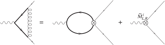
Figure 2.5: The matching at the scale $\mu=M$.

It is perhaps useful to think of the $\tilde{M}_{L,R}^{i}$ as the value that the coefficients of the effective Lagrangian take at the matching scale, as they contain the information on modes of frequencies $\mu>M$. The $\tilde{M}_{L,R}^{i}$ will be, in general, divergent, i.e. they will have a pole in $1/\epsilon$. Let us see how to obtain these coefficients $\tilde{M}_{L,R}^{i}$ in a particular case.

As discussed in the previous section we understand that at very high energies our theory is described by a gauge theory. Therefore we have to add to the Standard Model Lagrangian (already extended with technifermions) the following pieces

$$-\frac{1}{4}E_{\mu\nu}E^{\mu\nu}-\frac{1}{2}M^{2}E_{\mu}E^{\mu}+G\bar{Q}\gamma^{\mu}E_{\mu}q+\mathrm{h.c.}.$$ (2.74)

The $E_{\mu}$ vector boson (of mass $M$) acts in a large flavor group space which mixes ordinary fermions with heavy ones. (The notation in (2.74) is somewhat symbolic as we are not implying that the theory is vector-like, in fact we do not assume anything at all about it.)

At energies $\mu<M$ we can describe the contribution from this sector to the effective Lagrangian coefficients either using the degrees of freedom present in (2.74) or via the corresponding four quark operator and a non-zero value for the $\tilde{M}_{L,R}^{i}$ coefficients. Demanding that both descriptions reproduce the same renormalized $ffW$ vertex fixes the value of the $\tilde{M}_{L,R}^{i}$.

Let us see this explicitly in the case where the intermediate vector boson $E_{\mu}$ is a $SU(3)_{c}\times SU(2)_{L}$ singlet. For the sake of simplicity, we take the third term in (2.74) to be

$$G\bar{Q}_{L}\gamma^{\mu}E_{\mu}q_{L}.$$ (2.75)

At energies below $M$, the relevant four quark operator is then

$$-{\frac{G^{2}}{M^{2}}}(\bar{Q}_{L}\gamma^{\mu}q_{L})(\bar{q}_{L}\gamma_{\mu}Q_{L}).$$ (2.76)

In the limit of degenerate techniquark masses, it is quite clear that only $\tilde{M}_{L}^{1}$ can be different from zero. Thus, one does not need to worry about matching quark self-energies. Concerning the vertex (Fig. 2.5), we have to impose Eq. (2.24), where now

$$\Delta\Gamma\equiv\Gamma_{E}-\Gamma_{4Q}.$$ (2.77)

Namely, $\Delta\Gamma$ is the difference between the vertex computed using Eq. (2.74) and the same quantity computed using the four quark operators as well as non zero $\tilde{M}_{L,R}^{i}$ coefficients (recall that the hat in Eq. (2.24) denotes renormalized quantities). A calculation analogous to that of section 3 (now the leading terms in $1/M^{2}$ are retained) leads to

$$\tilde{M}_{L}^{1}=-{\frac{G^{2}}{16\pi^{2}}}{\frac{m_{Q}^{2}}{M^{2}}}{\frac{1}{\hat{\epsilon}}}.$$ (2.78)

7 Integrating out heavy fermions

As we move down in energies we can integrate lower and lower frequencies with the help of the four-fermion operators (which do accurately describe physics below $M$). This modifies the value of the $M_{L,R}^{i}$

$$M_{L,R}^{i}(\mu)=\tilde{M}_{L,R}^{i}+\Delta M_{L,R}^{i}(\mu/M),\qquad\mu<M.$$ (2.79)

The quantity $\Delta M_{L,R}^{i}(\mu/M)$ can be computed in perturbation theory down to the scale $\Lambda_{\chi}$ where the residual interactions labelled by the index $A$ becomes strong and confine the technifermions. The leading contribution is given by a loop of technifermions.

To determine such contribution it is necessary to demand that the renormalized Green functions match when computed using explicitly the degrees of freedom $Q_{L}$, $Q_{R}$ and when their effect is described via the effective Lagrangian coefficients $M_{L,R}^{i}$. The matching procedure is illustrated in Fig. 2.6.

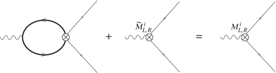
Figure 2.6: Matching at the scale $\mu=\Lambda_{\chi}$.

The scale $\mu$ of the matching must be such that $\mu<M$, but such that $\mu>\Lambda_{\chi}$, where perturbation theory in the technicolor coupling constant starts being questionable.

The result of the calculation in the case of degenerate masses is

$$\Delta M_{L,R}^{i}(\mu/M)=-\bar{M}_{L,R}^{i}\left(1-\hat{\epsilon}\log{\frac{\mu^{2}}{M^{2}}}\right),$$ (2.80)

where we have kept the logarithmically enhanced contribution only and have neglected any other possible constant pieces. $\bar{M}_{L,R}^{i}$ is the singular part of $\tilde{M}_{L,R}^{i}$. The finite parts of $\tilde{M}_{L,R}^{i}$ are clearly very model dependent (cf for instance the previous discussion on evanescent operators) and we cannot possibly take them into account in a general analysis. Accordingly, we ignore all other terms in (2.80) as well as those finite pieces generated through the fierzing procedure (see discussion in previous section). Keeping the logarithmically enhanced terms therefore sets the level of accuracy of our calculation. We will call (2.79) the short-distance contribution to the coefficient $M_{L,R}^{i}$. General formulae for the case where the two technifermions are not degenerate in masses can be found in appendix B.5.

Notice that the final short distance contribution to the $M_{L,R}^{i}$ is ultraviolet finite, as it should. The divergences in $\tilde{M}_{L,R}^{i}$ are exactly matched by those in $\Delta M_{L,R}^{i}$. The pole in $\tilde{M}_{L,R}^{i}$ combined with singularity in $\Delta M_{L,R}^{i}$ provides a finite contribution.

There is another potential source of corrections to the $M_{L,R}^{i}$ stemming from the renormalization of the four fermion coupling constant $G^{2}/M^{2}$ (similar to the renormalization of the Fermi constant in the electroweak theory due to gluon exchange). This effect is however subleading here. The reason is that we are considering technigluon exchange only for four-fermion operators of the form $\mathbf{J}\cdot\mathbf{j}$, where, again, $\mathbf{j}$ ($\mathbf{J}$) stands for a (heavy) fermion current (which give the leading contribution, as discussed). The fields carrying technicolor have the same handedness and thus there is no multiplicative renormalization and the effect is absent.

Of course in addition to the short distance contribution there is a long-distance contribution from the region of integration of momenta $\mu<\Lambda_{\chi}$. Perturbation theory in the technicolor coupling constant is questionable and we have to resort to other methods to determine the value of the $M_{L,R}^{i}$ at the $Z$ mass.

There are two possible ways of doing so. One is simply to mimic the constituent chiral quark model of QCD. There one loop of chiral quarks with momentum running between the scale of chiral symmetry breaking and the scale of the constituent mass of the quark, which acts as infrared cut-off, provide the bulk of the contribution [57, 58] to $f_{\pi}$, which is the equivalent of $v$. Making the necessary translations we can write for QCD-like theories

$$v^{2}\simeq n_{TC}n_{D}\frac{m_{Q}^{2}}{4\pi^{2}}\log\frac{\Lambda_{\chi}^{2}}{m_{Q}^{2}}.$$ (2.81)

Alternatively, we can use chiral Lagrangian techniques [62] to write a low-energy bosonized version of the technifermion bilinears $\bar{Q}_{L}\Gamma Q_{L}$ and $\bar{Q}_{R}\Gamma Q_{R}$ using the chiral currents $\mathbf{J}_{L}$ and $\mathbf{J}_{R}$. The translation is

$$\bar{Q}_{L}\gamma^{\mu}Q_{L} \rightarrow \frac{v^{2}}{2}\mathrm{tr}U^{\dagger}iD_{\mu}U$$ (2.82)

$$\bar{Q}_{L}\gamma^{\mu}\tau^{i}Q_{L} \rightarrow \frac{v^{2}}{2}\mathrm{tr}U^{\dagger}\tau^{i}iD_{\mu}U$$ (2.83)

$$\bar{Q}_{R}\gamma^{\mu}Q_{R} \rightarrow \frac{v^{2}}{2}\mathrm{tr}UiD_{\mu}U^{\dagger}$$ (2.84)

$$\bar{Q}_{R}\gamma^{\mu}\tau^{i}Q_{R} \rightarrow \frac{v^{2}}{2}\mathrm{tr}U\tau^{i}iD_{\mu}U^{\dagger}$$ (2.85)

Other currents do not contribute to the effective coefficients. Both methods agree.

Finally, we collect all contributions to the coefficients $M_{L,R}^{i}$ of the effective Lagrangian. For fields in the usual representations of the gauge group

$$2M_{L}^{1} = a_{\vec{L}^{2}}\frac{G^{2}}{M^{2}}(v^{2}+n_{TC}n_{D}\frac{m_{Q}^{2}}{4\pi^{2}}\log\frac{M^{2}}{\Lambda_{\chi}^{2}})-\frac{1}{16\pi^{2}}\frac{y_{u}^{2}+y_{d}^{2}}{4}(\frac{1}{\hat{\epsilon}}-\log\frac{\Lambda^{2}}{\mu^{2}}),$$ (2.86)

$$2M_{R}^{1} = (a_{\vec{R}^{2}}+\frac{1}{2}a_{R_{3}^{2}})\frac{G^{2}}{M^{2}}(v^{2}+n_{TC}n_{D}\frac{m_{Q}^{2}}{4\pi^{2}}\log\frac{M^{2}}{\Lambda_{\chi}^{2}})-\frac{1}{16\pi^{2}}\frac{(y_{u}+y_{d})^{2}}{8}(\frac{1}{\hat{\epsilon}}-\log\frac{\Lambda^{2}}{\mu^{2}}),$$ (2.87)

$$M_{L}^{2} = \frac{1}{2}a_{R_{3}L}\frac{G^{2}}{M^{2}}(v^{2}+n_{TC}n_{D}\frac{m_{Q}^{2}}{4\pi^{2}}\log\frac{M^{2}}{\Lambda_{\chi}^{2}})+\frac{1}{16\pi^{2}}\frac{y_{u}^{2}-y_{d}^{2}}{8}(\frac{1}{\hat{\epsilon}}-\log\frac{\Lambda^{2}}{\mu^{2}}),$$ (2.88)

$$2M_{L}^{3} = 0,$$ (2.89)

$$M_{R}^{2} = \frac{1}{2}a_{R_{3}R}\frac{G^{2}}{M^{2}}(v^{2}+n_{TC}n_{D}\frac{m_{Q}^{2}}{4\pi^{2}}\log\frac{M^{2}}{\Lambda_{\chi}^{2}})-\frac{1}{16\pi^{2}}\frac{y_{u}^{2}-y_{d}^{2}}{8}(\frac{1}{\hat{\epsilon}}-\log\frac{\Lambda^{2}}{\mu^{2}}),$$ (2.90)

$$2M_{R}^{3} = \frac{1}{2}a_{R_{3}^{2}}\frac{G^{2}}{M^{2}}(v^{2}+n_{TC}n_{D}\frac{m_{Q}^{2}}{4\pi^{2}}\log\frac{M^{2}}{\Lambda_{\chi}^{2}})-\frac{1}{16\pi^{2}}\frac{(y_{u}-y_{d})^{2}}{8}(\frac{1}{\hat{\epsilon}}-\log\frac{\Lambda^{2}}{\mu^{2}}),$$ (2.91)

while in the case of higher representations, where only custodially preserving operators have been considered, only $M_{L}^{1}$ and $M_{R}^{1}$ get non-zero values (through $a_{{\vec{L}}^{2}}$ and $a_{{\vec{R}}^{2}}$). The long distance contribution is, obviously, universal (see section 1), while we have to modify the short distance contribution by replacing the Casimir of the fundamental representation of $SU(2)$ for the appropriate one ($1/2\rightarrow c(R)$), the number of doublets by the multiplicity of the given representation, and $n_{c}$ by the appropriate dimensionality of the $SU(3)_{c}$ representation to which the $Q$ fields belong.

These expressions require several comments. First of all, they contain the same (universal) divergences as their counterparts in the minimal Standard Model. The scale $\Lambda$ should, in principle, correspond to the matching scale $\Lambda_{\chi}$, where the low-energy non-linear effective theory takes over. However, we write an arbitrary scale just to remind us that the finite part accompanying the log is regulator dependent and cannot be determined within the effective theory. Recall that the leading $\mathcal{O}(n_{TC}n_{D})$ term is finite and unambiguous, and that the ambiguity lies in the formally subleading term (which, however, due to the log is numerically quite important). Furthermore only logarithmically enhanced terms are included in the above expressions. Finally one should bear in mind that the chiral quark model techniques that we have used are accurate only in the large $n_{TC}$ expansion (actually $n_{TC}n_{D}$ here). The same comments apply of course to the oblique coefficients $a_{i}$ presented in appendix B.5.

The quantities $a_{\vec{L}^{2}}$, $a_{\vec{R}^{2}}$, $a_{R_{3}^{2}}$, $a_{R_{3}L}$ and $a_{R_{3}R}$ are the coefficients of the four-fermion operators indicated by the sub-index (a combination of Clebsch-Gordan and fierzing factors). They depend on the specific model. As discussed in previous sections these coefficients can be of either sign. This observation is important because it shows that the contribution to the effective coefficients has no definite sign [63] indeed. It is nice that there is almost a one-to-one correspondence between the effective Lagrangian coefficients (all of them measurable, at least in principle) and four-fermion coefficients.

Apart from these four-fermion coefficients, the $M_{L,R}^{i}$ depend on a number of quantities ($v$, $m_{Q}$, $\Lambda_{\chi}$, $G$ and $M$). Let us first discuss those related to the electroweak symmetry breaking, ($m_{Q}$ and $\Lambda_{\chi}$) and postpone the considerations on $M$ to the next section ($G$ will be assumed to be of $\mathcal{O}(1)$). $v$ is of course the Fermi scale and hence not an unknown at all ($v\simeq 250$ GeV). The value of $m_{Q}$ can be estimated from (2.81) since $v^{2}$ is known and $\Lambda_{\chi}$, for QCD-like technicolor theories is $\sim 4\pi v$. Solving for $m_{Q}$ one finds that if $n_{D}=4$, $m_{Q}\simeq v$, while if $n_{D}=1$, $m_{Q}\simeq 2.5v$. Notice that $m_{Q}$ and $v$ depend differently on $n_{TC}$ so it is not correct to simply assume $m_{Q}\simeq v$. In theories where the technicolor $\beta$ function is small (and it is pretty small if $n_{D}=4$ and $n_{TC}=2$) the characteristic scale of the breaking is pushed upwards, so we expect $\Lambda_{\chi}\gg 4\pi v$. This brings $m_{Q}$ somewhat downwards, but the decrease is only logarithmic. We shall therefore take $m_{Q}$ to be in the range 250 to 450 GeV. We shall allow for a mass splitting within the doublets too. The splitting within each doublet cannot be too large, as Fig. 2.4 shows. For simplicity we shall assume an equal splitting of masses for all doublets.

8 Results and discussion

Let us first summarize our results so far. The values of the effective Lagrangian coefficients encode the information about the symmetry breaking sector that is (and will be in the near future) experimentally accessible. The $M_{L,R}^{i}$ are therefore the counterpart of the oblique corrections coefficients $a_{i}$ and they have to be taken together in precision analysis of the Standard Model, even if they are numerically less significant.

These effective coefficients apply to $Z$-physics at LEP, top production at the Next Linear Collider, measurements of the top decay at CDF, or indeed any other process involving the third generation (where their effect is largest), provided the energy involved is below $4\pi v$, the limit of applicability of chiral techniques. (Of course chiral effective Lagrangian techniques fails well below $4\pi v$ if a resonance is present in a given channel, see also [64].)

In the Standard model the $M_{L,R}^{i}$ are useful to keep track of the $\log M_{H}$ dependence in all processes involving either neutral or charged currents. They also provide an economical description of the symmetry breaking sector, in the sense that they contain the relevant information in the low-energy regime, the only one testable at present. Beyond the Standard model the new physics contribution is parametrized by four-fermion operators. By choosing the number of doublets, $m_{Q}$, $M$, and $\Lambda_{\chi}$ suitably, we are in fact describing in a single shot a variety of theories: extended technicolor (commuting and non-commuting), walking technicolor [65] or top-assisted technicolor, provided that all remaining scalars and pseudo-Goldstone bosons are sufficiently heavy.

The accuracy of the calculation is limited by a number of approximations we have been forced to make and which have been discussed at length in previous sections. In practice we retain only terms which are logarithmically enhanced when running from $M$ to $m_{Q}$, including the long distance part, below $\Lambda_{\chi}$. The effective Lagrangian coefficients $M_{L,R}^{i}$ are all finite at the scale $\Lambda_{\chi}$, the lower limit of applicability of perturbation theory. Below that scale they run following the renormalization group equations of the non-linear theory and new divergences have to be subtracted. These coefficients contain finally the contribution from scales $M>\mu>m_{Q}$, the dynamically generated mass of the technifermion (expected to be of $\mathcal{O}(\Lambda_{TC})$). In view of the theoretical uncertainties, to restrict oneself to logarithmically enhanced terms is a very reasonable approximation which should capture the bulk of the contribution.

Let us now proceed to a more detailed discussion of the implications of our analysis. Let us begin by discussing the value that we should take for $M$, the mass scale normalizing four-fermion operators. Fermion condensation gives a mass to ordinary fermions via chirality-flipping operators of order

$$m_{f}\simeq\frac{G^{2}}{M^{2}}\langle\bar{Q}Q\rangle,$$ (2.92)

through the operators listed in table 2.2. A chiral quark model calculation shows that

$$\langle\bar{Q}Q\rangle\simeq v^{2}m_{Q}.$$ (2.93)

Thus, while $\langle\bar{Q}Q\rangle$ is universal, there is an inverse relation between $M^{2}$ and $m_{f}$. In QCD-like theories this leads to the following rough estimates for the mass $M$ (the subindex refers to the fermion which has been used in the l.h.s. of (2.92))

$$M_{e}\sim 150\mathrm{TeV},\qquad M_{\mu}\sim 10\mathrm{TeV},\qquad M_{b}\sim 3\mathrm{TeV}.$$ (2.94)

If taken at face value, the scale for $M_{b}$ is too low, even the one for $M_{\mu}$ may already conflict with current bounds on FCNC, unless they are suppressed by some other mechanism in a natural way. Worse, the top mass cannot be reasonably reproduced by this mechanism. This well-known problem can be partly alleviated in theories where technicolor walks or invoking top-color or a similar mechanism [66]). Then $M$ can be made larger and $m_{Q}$, as discussed, somewhat smaller. For theories which are not vector-like the above estimates become a lot less reliable.

However one should not forget that none of the four-fermion operators playing a role in the vertex effective couplings participates at all in the fermion mass determination. In principle we can then entertain the possibility that the relevant mass scale for the latter should be lower (perhaps because they get a contribution through scalar exchange, as some of them can be generated this way). Even in this case it seems just natural that $M_{b}$ (the scale normalizing chirality preserving operators for the third generation, that is) is low and not too different from $\Lambda_{\chi}$. Thus the logarithmic enhancement is pretty much absent in this case and some of the approximations made become quite questionable in this case. (Although even for the $b$ couplings there is still a relatively large contribution to the $M_{L,R}^{i}$’s coming from long distance contributions.) Put in another words, unless an additional mechanism is invoked, it is not really possible to make definite estimates for the $b$-effective couplings without getting into the details of the underlying theory. The flavor dynamics and electroweak breaking are completely entangled in this case. If one only retains the long distance part (which is what we have done in practice) we can, at best, make order-of-magnitude estimates. However, what is remarkable in a way is that this does not happen for the first and second generation vertex corrections. The effect of flavor dynamics can then be encoded in a small number of coefficients.

We shall now discuss in some detail the numerical consequences of our assumptions. We shall assume the above values for the mass scale $M$; in other words, we shall place ourselves in the most disfavored situation. We shall only present results for QCD-like theories and $n_{D}=4$ exclusively. For other theories the appropriate results can be very easily obtained from our formulae. For the coefficients $a_{\vec{L}^{2}}$, $a_{R_{3}R}$, $a_{R_{3}L}$, etc. we shall use the range of variation [-2, 2] (since they are expected to be of $\mathcal{O}(1)$). Of course larger values of the scale, $M$, would simply translate into smaller values for those coefficients, so the results can be easily scaled down.

Fig. 2.7 shows the $g_{A}^{e},g_{V}^{e}$ electron effective couplings when vertex corrections are included and allowed to vary within the stated limits. To avoid clutter, the top mass is taken to the central value 175.6 GeV. The Standard Model prediction is shown as a function of the Higgs mass. The dotted lines in Fig. 2.7 correspond to considering the oblique corrections only. Vertex corrections change these results and, depending on the values of the four-fermion operator coefficients, the prediction can take any value in the strip limited by the two solid lines (as usual we have no specific prediction in the direction along the strip due to the dependence on $\Lambda$, inherited from the non-renormalizable character of the effective theory). A generic modification of the electron couplings is of $\mathcal{O}(10^{-5})$, small but much larger than in the Standard Model and, depending on its sign, may help to bring a better agreement with the central value.

The modifications are more dramatic in the case of the second generation, for the muon, for instance. Now, we expect changes in the $M_{L,R}^{i}$’s and, eventually, in the effective couplings of $\mathcal{O}(10^{-3})$ These modifications are just at the limit of being observable. They could even modify the relation between $M_{W}$ and $G_{\mu}$ (i.e. $\Delta r$).

Fig. 2.8 shows a similar plot for the bottom effective couplings $g_{A}^{b},g_{V}^{b}$. It is obvious that taking generic values for the four-fermion operators (of $\mathcal{O}(1)$) leads to enormous modifications in the effective couplings, unacceptably large in fact. The corrections become more manageable if we allow for a smaller variation of the four-fermion operator coefficients (in the range [-0.1,0.1]). This suggests that the natural order of magnitude for the mass $M_{b}$ is $\sim 10$ TeV, at least for chirality preserving operators. As we have discussed the corrections can be of either sign.

Figure 2.7: Oblique and vertex corrections for the electron effective couplings. The elipse indicate the 1-$\sigma$ experimental region. Three values of the effective mass $m_{2}$ are considered: 250 (a), 350 (b) and 450 GeV (c), and two splittings: 10% (right) and 20% (left). The dotted lines correspond to including the oblique corrections only. The coefficients of the four-fermion operators vary in the range [-2,2] and this spans the region between the two solid lines. The Standard Model prediction (thick solid line) is shown for $m_{t}=175.6$ GeV and $70\leq M_{H}\leq 1500$ GeV.

Figure 2.8: Bottom effective couplings compared to the SM prediction for $m_{t}=175.6$ as a function of the Higgs mass (in the range [70,1500] GeV). The elipses indicate 1, 2, and 3-$\sigma$ experimental regions. The dynamically generated masses are 250 (a), 350 (b) and 400 GeV (c) and we show a 20% splitting between the masses in the heavy doublet. The degenerate case does not present quantitative differencies if we consider the experimental errors. The central lines correspond to including only the oblique corrections. When we include the vertex corrections (depending on the size of the four-fermion coefficients) we predict the regions between lines indicated by the arrows. The four-fermion coefficients in this case take values in the range [-0.1,0.1].

One could, at least in the case of degenerate masses, translate the experimental constraints on the $M_{L,R}^{i}$ (recall that their experimental determination requires a combination of charged and neutral processes, since there are six of them) to the coefficients of the four-fermion operators. Doing so would provide us with a four-fermion effective theory that would exactly reproduce all the available data. It is obvious however that the result would not be very satisfactory. While the outcome would, most likely, be coefficients of $\mathcal{O}(1)$ for the electron couplings, they would have to be of $\mathcal{O}(10^{-1})$, perhaps smaller for the bottom. Worse, the same masses we have used lead to unacceptably low values for the top mass (2.92). Allowing for a different scale in the chirality flipping operators would permit a large top mass without affecting the effective couplings. Taking this as a tentative possibility we can pose the following problem: measure the effective couplings $M_{L,R}^{i}$ for all three generations and determine the values of the four-fermion operator coefficients and the characteristic mass scale that fits the data best. In the degenerate mass limit we have a total of 8 unknowns (5 of them coefficients, expected to be of $\mathcal{O}(1)$) and 18 experimental values (three sets of the $M_{L,R}^{i}$). A similar exercise could be attempted in the chirality flipping sector. If the solution to this exercise turned out to be mathematically consistent (within the experimental errors) it would be extremely interesting. A negative result would certainly rule out this approach. Notice that dynamical symmetry breaking predicts the pattern $M_{L,R}^{i}\sim m_{f}$, while in the Standard Model $M_{L,R}^{i}\sim m_{f}^{2}$.

We should end with some words of self-criticism. It may seem that the previous discussion is not too conclusive and that we have managed only to rephrase some of the long-standing problems in the symmetry breaking sector. However, the raison d’être of the present work is not really to propose a solution to these problems, but rather to establish a theoretical framework to treat them systematically. Experience from the past shows that often the effects of new physics are magnified and thus models are ruled out on this basis, only to find out that a careful and rigorous analysis leaves some room for them. We believe that this may be the case in dynamical symmetry breaking models and we believe too that only through a detailed and careful comparison with the experimental data will progress take place.

The effective Lagrangian provides the tools to look for an ‘existence proof’ (or otherwise) of a phenomenologically viable, mathematically consistent dynamical symmetry breaking model. We hope that there is any time soon sufficient experimental data to attempt to determine the four-fermion coefficients, at lest approximately.

Chapter 3 $CP$ violation and mixing

One of the pressing open problems in particle physics is to understand the origin of $CP$ violation and family mixing. In the minimal Standard Model we have only two possible sources of $CP$ violation, one is the strong $CP$ phase controlling the gluonic topological term and the other is the single phase present in the so-called Cabibbo-Kobayashi-Maskawa (CKM) mixing matrix (here denoted $K$) in the electroweak sector. In this chapter we will deal only with the electroweak sector even though both sectors are related [3].

Our main purpose here is to parametrize all possible sources of $CP$ violation and family mixing that may arise in the electroweak sector when considering new physics beyond the SM using an effective Lagrangian approach. Like in the previous chapter we consider only leading four-dimensional operators keeping all fields of the SM, except the not yet observed Higgs field. We start with a general classification of four-dimensional operators respecting the $SU(3)_{c}\times SU(2)_{L}\times U(1)_{Y}$ gauge symmetry with matter and gauge fields in the standard representations. This classification includes non-diagonal kinetic and mass terms along with Appelquist et al. effective operators. We perform a diagonalization in section 2 showing that, besides the presence of the CKM matrix in the SM charged vertex, new structures show up in effective operators constructed with left handed fermions. The rest of the chapter is dedicated to the study of the contribution of the effective operators to the physical observables in the neutral and charged vertices. Care is taken to ensure that all contributions to the observable quantities are taken into account, including wave function and CKM renormalization that are present even at tree level. The final section is devoted to the analysis of the SM supplemented with an additional heavy fermion doublet and the case of the SM with a heavy Higgs.

1 Effective Lagrangian and $CP$ violation

Let us first state the assumptions behind the present framework. We shall assume that the scale of any new physics beyond the standard model is sufficiently high so that an inverse mass expansion is granted, and we shall organize the effective Lagrangian accordingly. We shall also assume that the Higgs field either does not exist or is massive enough to permit an effective Lagrangian treatment by expanding in inverse powers of its mass, $M_{H}$. In short, we assume that all as yet undetected new particles are heavy, with a mass much larger than the energy scale at which the effective Lagrangian is to be used. Thus it is natural to use a non-linear realization of the $SU(2)_{L}\times U(1)$ symmetry where the unphysical scalar fields are collected in a unitary $2\times 2$ matrix $U(x)$ (see e.g. [39]).

An additional assumption that we shall later make is that whatever is the source of $CP$-violation beyond the Standard Model, when compared to the $CP$ conserving part, is ‘small’. This statement does need qualification. What we actually mean is that observable $CP$ violating deviations must me small. This does not mean that $CP$-violating operators are always suppressed. We can have the situation where lots of $CP$ violating phases appear or disappear when we pass to the physical basis. Since this basis is the most directly related one to observable quantities it is the chosen one to make a qualitative and quantitative analysis of $CP$ violating effects. However, we always have to remember that observable quantities include in their calculation renormalization contributions along with finite renormalizations of the involved external fields which generically alter the weight of the different $CP$ violating operators as we shall see.

Let us commence our classification of the operators present in the matter sector of the effective electroweak Lagrangian. We shall use the following projectors

$$R=\frac{1+\gamma^{5}}{2},\qquad L=\frac{1+\gamma^{5}}{2}\qquad\tau^{u}=\frac{1+\tau^{3}}{2},\qquad\tau^{d}=\frac{1-\tau^{3}}{2},$$ (3.1)

where $R$ is the right projector and $L$ the left projector in chirality space, and $\tau^{u}$ is the up projector and $\tau^{d}$ the down projector in $SU(2)$ space. The different gauge groups act on the scalar, $U(x)$, and fermionic, $f_{L}(x),f_{R}(x)$, fields in the following way

$$D_{\mu}U = \partial_{\mu}U+ig\frac{\tau}{2}\cdot W_{\mu}U-ig^{\prime}U\frac{\tau^{3}}{2}B_{\mu},$$

$$D_{\mu}^{L}f_{L} = \left[\partial_{\mu}+ig\frac{\tau}{2}\cdot W_{\mu}+ig^{\prime}\left(Q-\frac{\tau^{3}}{2}\right)B_{\mu}+ig_{s}\frac{\lambda}{2}\cdot G_{\mu}\right]f_{L},$$

$$D_{\mu}^{R}f_{R} = \left[\partial_{\mu}+ig^{\prime}QB_{\mu}+ig_{s}\frac{\lambda}{2}\cdot G_{\mu}\right]f_{R},$$ (3.2)

with

$$Q=\left\{\begin{array}[]{ccc}\frac{\tau^{3}}{2}+\frac{1}{6}&&\mathrm{quarks}\\ \frac{\tau^{3}}{2}-\frac{1}{2}&&\mathrm{leptons}\end{array}\right..$$

The following terms are universal. They must be present in any effective theory whose long-distance properties are those of the Standard Model. They correspond to the Standard Model kinetic and mass terms (we use the notation $\mathrm{f}$ to describe both left and right degrees of freedom simultaneously)

$$\mathcal{L}_{kin}^{L} = i\mathrm{\bar{f}}X_{L}\gamma^{\mu}D_{\mu}^{L}L\mathrm{f},$$

$$\mathcal{L}_{kin}^{R} = i\mathrm{\bar{f}}\left(\tau^{u}X_{R}^{u}+\tau^{d}X_{R}^{d}\right)\gamma^{\mu}D_{\mu}^{R}R\mathrm{f},$$

$$\mathcal{L}_{m} = -\mathrm{\bar{f}}\left(U\left(\tau^{u}\tilde{y}_{u}^{f}+\tau^{d}\tilde{y}_{d}^{f}\right)R+\left(\tau^{u}\tilde{y}_{u}^{f\dagger}+\tau^{d}\tilde{y}_{d}^{f\dagger}\right)U^{\dagger}L\right)\mathrm{f},$$ (3.3)

where $X_{L}$, $X_{R}^{u}$ and $X_{R}^{d}$ are non-singular Hermitian matrices having only family indices, and $\tilde{y}_{u}^{f}$ and $\tilde{y}_{d}^{f}$ are arbitrary matrices and have only family indices too. Note that in general $X_{R}^{d}\neq X_{R}^{u}$ and therefore the operator $\mathcal{L}_{R}^{\prime}$ presented in the previous chapter is automatically incorporated in these terms . In the Standard Model, these matrices can always be reabsorbed by an appropriate redefinition of the fields (we shall see this explicitly later), so one does not even contemplate the possibility that left and right ‘kinetic’ terms are differently normalized, but this is perfectly possible in an effective theory, and the transformations required to bring these kinetic terms to the standard form do leave some fingerprints.

In order to write the above terms in the familiar form in the Standard Model we shall perform a series of chiral changes of variables. In general, due to the axial anomaly, these changes will modify the topological $CP$ violating $\theta$-terms

$$\mathcal{L}_{\theta}=\epsilon^{\alpha\beta\mu\nu}\left(\theta_{1}B_{\alpha\beta}B_{\mu\nu}+\theta_{2}W_{\alpha\beta}^{a}W_{\mu\nu}^{a}+\theta_{3}G_{\alpha\beta}^{a}G_{\mu\nu}^{a}\right).$$ (3.4)

From those terms only the gluonic $\theta$-term is observable [67] but we will not deal here with this issue.

Notice the appearance of the unitary matrix $U$ collecting the (unphysical) Goldstone bosons. The Higgs field —as emphasized above— should it exist, has been integrated out. Since the global symmetries are non-linearly realized the above Lagrangian is non-renormalizable and additional operators are required to absorb the additional divergences which are generated due to the non-linear nature of the theory.

In addition to (3.3) a number of operators of dimension four should be included in the matter sector of the effective electroweak Lagrangian. They are, to begin with, necessary as counterterms to remove some ultraviolet divergences that appear at the quantum level due to the non-linear nature of (3.3). Moreover, physics beyond the Standard Model does in general contribute to the coefficients of those operators, as it may do to $X_{L}$, $X_{Ru}$ $X_{Rd}$, $\tilde{y}_{u}$ and $\tilde{y}_{d}$. The dimension 4 operators can be written generically as

$$\mathcal{L}_{L} = \mathrm{\bar{f}}\gamma_{\mu}M_{L}O_{L}^{\mu}L\mathrm{f}+h.c.,$$

$$\mathcal{L}_{R} = \mathrm{\bar{f}}\gamma_{\mu}M_{R}O_{R}^{\mu}R\mathrm{f}+h.c.,$$ (3.5)

where $M_{L}$ and $M_{R}$ are matrices having family indices only and $O_{L}^{\mu}$ and $O_{R}^{\mu}$ are operators of dimension one having weak indices (u,d) only. These operators were first written by [39] in the case where mixing between families is absent and they have been recently considered in [68]. The extension to the three-generation case is new and presented here.

The complete list of the dimension four operators is

$$\mathcal{L}_{L}^{1} = i\mathrm{\bar{f}}M_{L}^{1}\gamma^{\mu}U\left(D_{\mu}U\right)^{\dagger}L\mathrm{f}+h.c.,$$

$$\mathcal{L}_{L}^{2} = i\mathrm{\bar{f}}M_{L}^{2}\gamma^{\mu}\left(D_{\mu}U\right)\tau^{3}U^{\dagger}L\mathrm{f}+h.c.$$

$$\mathcal{L}_{L}^{3} = i\mathrm{\bar{f}}M_{L}^{3}\gamma^{\mu}U\tau^{3}U^{\dagger}\left(D_{\mu}U\right)\tau^{3}U^{\dagger}L\mathrm{f}+h.c.,$$

$$\mathcal{L}_{L}^{4} = i\mathrm{\bar{f}}M_{L}^{4}\gamma^{\mu}U\tau^{3}U^{\dagger}D_{\mu}^{L}L\mathrm{f}+h.c..$$

$$\mathcal{L}_{R}^{1} = i\mathrm{\bar{f}}M_{R}^{1}\gamma^{\mu}U^{\dagger}\left(D_{\mu}U\right)R\mathrm{f}+h.c.,$$

$$\mathcal{L}_{R}^{2} = i\mathrm{\bar{f}}M_{R}^{2}\gamma^{\mu}\tau^{3}U^{\dagger}\left(D_{\mu}U\right)R\mathrm{f}+h.c.,$$

$$\mathcal{L}_{R}^{3} = i\mathrm{\bar{f}}M_{R}^{3}\gamma^{\mu}\tau^{3}U^{\dagger}\left(D_{\mu}U\right)\tau^{3}R\mathrm{f}+h.c.,$$ (3.6)

Without any loss of generality we take the matrices in family space $M_{L}^{1}$, $M_{R}^{1}$, $M_{L}^{3}$ and $M_{R}^{3}$ Hermitian, while $M_{L}^{2}$, $M_{R}^{2}$ and $M_{L}^{4}$ are completely general. If we require the above operators to be $CP$ conserving, the matrices $M_{LR}^{i}$ must be real (see section 5).

In addition to the above ones, physics beyond the Standard Model generates, in general, an infinite tower of higher-dimensional operators with $d\geq 5$ (these operators are eventually required as counterterms too due to the non-linear nature of the Lagrangian (3.3) ). On dimensional grounds these operators shall be suppressed by powers of the scale $\Lambda$ characterizing new physics or by powers of $4\pi v$ ($v$ being the scale of the breaking —250 GeV). Therefore, if the scale of new physics is sufficiently high the contribution of higher dimensional operators can be neglected as compared to those of $d=4$. Of course for this to be true the later must be non-vanishing and sizeable. Thanks to the violation of the Appelquist-Carazzone decoupling theorem[69] in spontaneously broken theories, this is generically the case, unless the new physics is tuned so as to be decoupling as is the case in the minimal supersymmetric Standard Model. Our results do not apply in this case (see e.g. [70] for a recent discussion on this matter).

2 Passage to the physical basis

Let us first consider the operators which are already present in the Standard Model, Eq. (3.3). The diagonalization and passage to the physical basis are of course well known, but some modifications are required when one considers the general case in (3.3) so it is worth going through the discussion with some detail.

We perform first the unitary change of variables

$$\mathrm{f}=\left[\tilde{V}_{L}L+\left(\tilde{V}_{Ru}\tau^{u}+\tilde{V}_{Rd}\tau^{d}\right)R\right]\mathrm{f},$$ (3.7)

with the help of the unitary matrices $\tilde{V}_{L}$ ,$\tilde{V}_{Ru}$ and $\tilde{V}_{Rd}$. Hence

$$\left(\tilde{y}_{u}^{f}\tau^{u}+\tilde{y}_{d}^{f}\tau^{d}\right)\rightarrow\left(\tilde{V}_{L}^{\dagger}\tilde{y}_{u}^{f}\tilde{V}_{Ru}\tau^{u}+\tilde{V}_{L}^{\dagger}\tilde{y}_{d}^{f}\tilde{V}_{Rd}\tau^{d}\right),$$ (3.8)

and

$$X_{L} \rightarrow \tilde{V}_{L}^{\dagger}X_{L}\tilde{V}_{L}=D^{L},$$

$$X_{R}^{u} \rightarrow \tilde{V}_{Ru}^{\dagger}X_{R}^{u}\tilde{V}_{Ru}=D_{u}^{R},$$

$$X_{R}^{d} \rightarrow \tilde{V}_{Rd}^{\dagger}X_{R}^{d}\tilde{V}_{Rd}=D_{d}^{R},$$ (3.9)

where $D^{L}$ $D_{u}^{R}$ and $D_{d}^{R}$ are diagonal matrices with eigenvalues different from zero. Then, with the help of a non-unitary transformation

$$\mathrm{f}\rightarrow\left[\left(D^{L}\right)^{-\frac{1}{2}}L+\left(\left(D_{u}^{R}\right)^{-\frac{1}{2}}\tau^{u}+\left(D_{d}^{R}\right)^{-\frac{1}{2}}\tau^{d}\right)R\right]\mathrm{f},$$ (3.10)

we obtain

$$D^{L} \rightarrow \left(\left(D^{L}\right)^{-\frac{1}{2}}\right)^{\ast}D^{L}\left(D^{L}\right)^{-\frac{1}{2}}=I,$$

$$D_{u}^{R} \rightarrow \left(\left(D_{u}^{R}\right)^{-\frac{1}{2}}\right)^{\ast}D_{u}^{R}\left(D_{u}^{R}\right)^{-\frac{1}{2}}=I,$$

$$D_{d}^{R} \rightarrow \left(\left(D_{d}^{R}\right)^{-\frac{1}{2}}\right)^{\ast}D_{d}^{R}\left(D_{d}^{R}\right)^{-\frac{1}{2}}=I,$$ (3.11)

and the matrix $\tilde{y}_{u}^{f}\tau^{u}+\tilde{y}_{d}^{f}\tau^{d}$ transforms into

$$\left(\left(D^{L}\right)^{-\frac{1}{2}}\right)^{\ast}\tilde{V}_{L}^{\dagger}\tilde{y}_{u}^{f}\tilde{V}_{Ru}\left(D_{u}^{R}\right)^{-\frac{1}{2}}\tau^{u}+\left(\left(D^{L}\right)^{-\frac{1}{2}}\right)^{\ast}\tilde{V}_{L}^{\dagger}\tilde{y}_{d}^{f}\tilde{V}_{Rd}\left(D_{d}^{R}\right)^{-\frac{1}{2}}\tau^{d}\equiv y_{u}^{f}\tau^{u}+y_{d}^{f}\tau^{d},$$ (3.12)

where $y_{u}^{f}$ and $y_{d}^{f}$ are the Yukawa couplings. Thus, the left and right kinetic terms can be brought to the canonical form at the sole expense of redefining the Yukawa couplings. Since this is all there is in the Standard Model, we see that the effect of considering more general coefficients for the right-handed kinetic terms is irrelevant. This will not be the case when additional operators are considered. Fermions transform, up to this point, in irreducible representations of the gauge group.

We now perform the unitary change of variables

$$\mathrm{f}\rightarrow\left[\left(V_{Lu}\tau^{u}+V_{Ld}\tau^{d}\right)L+\left(V_{Ru}\tau^{u}+V_{Rd}\tau^{d}\right)R\right]\mathrm{f},$$ (3.13)

with unitary matrices $V_{Lu}$, $V_{Ru}$, $V_{Ld}$ and $V_{Rd}$ and having family indices only. They are chosen so that the Yukawa terms become diagonal and definite positive (see [71])

$$\left(V_{Lu}^{\dagger}\tau^{u}+V_{Ld}^{\dagger}\tau^{d}\right)\left(y_{u}^{f}\tau^{u}+y_{d}^{f}\tau^{d}\right)\left(V_{Ru}\tau^{u}+V_{Rd}\tau^{d}\right)=d_{u}^{f}\tau^{u}+d_{d}^{f}\tau^{d}.$$ (3.14)

After all these transformations $\mathcal{L}_{m}$ transforms into

$$\mathcal{L}_{m}=-\mathrm{\bar{f}}\left\{\left(\tau^{u}U+K^{\dagger}\tau^{d}U\right)\tau^{u}d_{u}^{f}+\left(\tau^{d}U+K\tau^{u}U\right)\tau^{d}d_{d}^{f}\right\}R\mathrm{f}+h.c.,$$ (3.15)

where $K\equiv V_{Lu}^{\dagger}V_{Ld}$ is well known Cabibbo-Kobayashi-Maskawa matrix. Note in Eq. (3.15) that when we set $U=I$ we obtain

$$\mathcal{L}_{m}\rightarrow-\mathrm{\bar{f}}\left(\tau^{u}d_{u}^{f}+\tau^{d}d_{d}^{f}\right)R\mathrm{f}+h.c.,$$

which is a diagonal mass term. Fermions now transform in reducible representations of the gauge group.

The left and right kinetic terms now read

$$\mathcal{L}_{kin}^{R}=i\mathrm{\bar{f}}\gamma^{\mu}D_{\mu}^{R}R\mathrm{f},$$ (3.16)

and

$$\mathcal{L}_{kin}^{L} = i\mathrm{\bar{f}}\gamma^{\mu}L\left\{\partial_{\mu}+ig^{\prime}\left(Q-\frac{\tau^{3}}{2}\right)B_{\mu}+ig\frac{\tau^{3}}{2}W_{\mu}^{3}\right.$$ (3.17)

$$\left.+ig\left(K\frac{\tau^{-}}{2}W_{\mu}^{+}+K^{\dagger}\frac{\tau^{+}}{2}W_{\mu}^{-}\right)+ig_{s}\frac{\lambda}{2}\cdot G_{\mu}\right\}\mathrm{f}.$$

$CP$ violation is obtained if and only if $K\neq K^{\ast}$. In total the SM kinetic term is written using physical gauge bosons is given by

$$\mathcal{L}_{kin} = \mathcal{L}_{kin}^{L}+\mathcal{L}_{kin}^{R}=i\bar{f}\gamma^{\mu}\left\{\partial_{\mu}+ig_{s}\frac{\mathbf{\lambda}}{2}\mathbf{\cdot G}_{\mu}+ieQA_{\mu}\right.$$ (3.18)

$$+\left.\frac{ie}{s_{W}c_{W}}\left[\left(\frac{\tau^{3}}{2}-Qs_{W}^{2}\right)L-Qs_{W}^{2}R\right]Z_{\mu}\right\}f$$

$$-\frac{e}{\sqrt{2}s_{W}}\left[\bar{u}\gamma^{\mu}KW_{\mu}^{+}Ld+\bar{d}\gamma^{\mu}K^{\dagger}W_{\mu}^{-}Lu\right].$$

As is well known, some freedom for additional phase redefinitions is left. If we make the replacement

$$\mathrm{f}\rightarrow\left[\left(W_{Lu}\tau^{u}+W_{Ld}\tau^{d}\right)L+\left(W_{Ru}\tau^{u}+W_{Rd}\tau^{d}\right)R\right]\mathrm{f},$$ (3.19)

we have to change

$$K=V_{Lu}^{\dagger}V_{Ld}\rightarrow W_{Lu}^{\dagger}V_{Lu}^{\dagger}V_{Ld}W_{Ld}=W_{Lu}^{\dagger}KW_{Ld},$$ (3.20)

and

$$d_{u} = V_{Lu}^{\dagger}y_{u}^{f}V_{Ru}\rightarrow W_{Lu}^{\dagger}V_{Lu}^{\dagger}y_{u}^{f}V_{Ru}W_{Ru}=W_{Lu}^{\dagger}d_{u}^{f}W_{Ru},$$

$$d_{d} = V_{Ld}^{\dagger}y_{d}^{f}V_{Rd}\rightarrow W_{Ld}^{\dagger}V_{Ld}^{\dagger}y_{d}^{f}V_{Rd}W_{Rd}=W_{Ld}^{\dagger}d_{d}^{f}W_{Rd},$$ (3.21)

but if we want to keep $d_{u}^{f}$ and $d_{d}^{f}$ diagonal real and definite positive, and if we suppose that they do not have degenerate eigenstates the only possibility for the unitary matrices $W$ is to be diagonal. This freedom can be used, for example, to extract five phases from $K$. After this no further redefinitions are possible neither in the left nor in the right handed sector. Henceforth, without any loss of generality, we will absorb matrices $W$ in the definition of matrices $V$.

So much for the Standard Model. Let us now move to the more general case represented at low energies by the $d=4$ operators listed in the previous section. We have to analyze the effect of the transformations given by Eqs. (3.7) (3.10) and (3.13) on the operators (3.6). The composition of those transformations is given by

$$\mathrm{f} \rightarrow \tilde{V}_{L}\left(D^{L}\right)^{\frac{-1}{2}}\left(V_{Lu}\tau^{u}+V_{Ld}\tau^{d}\right)L\mathrm{f}$$ (3.22)

$$+\left(\tilde{V}_{Ru}\left(D_{u}^{R}\right)^{\frac{-1}{2}}V_{Ru}\tau^{u}+\tilde{V}_{Rd}\left(D_{d}^{R}\right)^{\frac{-1}{2}}V_{Rd}\tau^{d}\right)R\mathrm{f}$$

$$\equiv \left(C_{L}^{u}\tau^{u}+C_{L}^{d}\tau^{d}\right)L\mathrm{f}+\left(C_{R}^{u}\tau^{u}+C_{R}^{d}\tau^{d}\right)R\mathrm{f},$$

Note that because of the presence of matrices $D$, matrices $C$ are in general non-unitary. We begin with the effective operators involving left handed fields. In this case when we perform transformation (3.22) we obtain

$$\mathcal{L}_{L}\rightarrow\mathrm{\bar{f}}\gamma_{\mu}Q_{L}^{\mu}L\mathrm{f}+h.c.,$$ (3.23)

with the operator $Q_{L}^{\mu}$ containing family and weak indices given by

$$Q_{L}^{\mu} = \hat{M}_{L}\tau^{u}O_{L}^{\mu}\tau^{u}+\hat{M}_{L}K\tau^{u}O_{L}^{\mu}\tau^{d}$$ (3.24)

$$+K^{\dagger}\hat{M}_{L}K\tau^{d}O_{L}^{\mu}\tau^{d}+K^{\dagger}\hat{M}_{L}\tau^{d}O_{L}^{\mu}\tau^{u},$$

where we have defined

$$\hat{M}_{L}\equiv C_{L}^{u\dagger}M_{L}C_{L}^{u}.$$ (3.25)

Thus new structures do appear involving the CKM matrix $K$ and left-handed fields. The former cannot be reduced to our starting set of operators by a simple redefinition of the original couplings $M_{L}$.

The case of the effective operators involving right handed fields ($\mathcal{L}_{R}$) is, in this sense, simpler because transformation (3.22) only redefine the matrices $M_{R}$. The operators involving right-handed fields are $\mathcal{L}_{R}^{1}$, $\mathcal{L}_{R}^{2}$, and $\mathcal{L}_{R}^{3}$ and can be written generically as (see next section)

$$\mathcal{L}_{R}^{p}=i\mathrm{\bar{f}}\gamma_{\mu}M_{R}^{p}O_{p}^{\mu}R\mathrm{f}+h.c.,$$ (3.26)

with

$$O_{1}^{\mu}=U^{\dagger}\left(D_{\mu}U\right),\qquad O_{2}^{\mu}=\tau^{3}U^{\dagger}\left(D_{\mu}U\right),\qquad O_{3}^{\mu}=\tau^{3}U^{\dagger}\left(D_{\mu}U\right)\tau^{3}.$$ (3.27)

Note that because of the $h.c.$ in $\mathcal{L}_{R}^{p}$ we can change $O_{2}^{\mu}$ by $U^{\dagger}\left(D_{\mu}U\right)\tau^{3}$ along with $M_{R}^{2}$ by $M_{R}^{2\dagger}$. So under the transformation (3.22) we obtain

$$\mathcal{L}_{R}^{p}\rightarrow i\mathrm{\bar{f}}\gamma_{\mu}Q_{pR}^{\mu}R\mathrm{f}+h.c.,$$

with the operators $Q_{pR}^{\mu}$ containing family and weak indices given by

$$Q_{pR}^{\mu} = C_{R}^{u\dagger}M_{R}^{p}C_{R}^{u}\tau^{u}O_{p}^{\mu}\tau^{u}+C_{R}^{u\dagger}M_{R}^{p}C_{R}^{d}\tau^{u}O_{p}^{\mu}\tau^{d}$$ (3.28)

$$+C_{R}^{u\dagger}M_{R}^{p}C_{R}^{d}\tau^{d}O_{p}^{\mu}\tau^{d}+C_{R}^{d\dagger}M_{R}^{p}C_{R}^{u}\tau^{d}O_{p}^{\mu}\tau^{u},$$

hence

$$\sum_{p=1}^{3}\mathcal{L}_{R}^{p} \rightarrow \sum_{p=1}^{3}\left(i\mathrm{\bar{f}}\gamma_{\mu}Q_{pR}^{\mu}R\mathrm{f}+h.c.\right)$$ (3.29)

$$= \sum_{p=1}^{3}\left(i\mathrm{\bar{f}}\gamma_{\mu}\tilde{M}_{R}^{p}O_{p}^{\mu}R\mathrm{f}+h.c.\right),$$

with

$$\hat{M}_{R}^{1} = C_{+}^{\dagger}M_{R}^{1}C_{+}+C_{-}^{\dagger}M_{R}^{2}C_{+}+C_{-}^{\dagger}M_{R}^{3}C_{-},$$

$$\hat{M}_{R}^{2} = C_{-}^{\dagger}M_{R}^{1}C_{+}+C_{+}^{\dagger}M_{R}^{2}C_{+}+C_{+}^{\dagger}M_{R}^{3}C_{-},$$

$$\hat{M}_{R}^{3} = C_{-}^{\dagger}M_{R}^{1}C_{-}+C_{+}^{\dagger}M_{R}^{2}C_{-}+C_{+}^{\dagger}M_{R}^{3}C_{+},$$ (3.30)

where $C_{\pm}=(C_{R}^{u}\pm C_{R}^{d})/2$. Hence, transformations (3.22) can be absorbed by a mere redefinition of the matrices$\ M_{R}^{1},$ $M_{R}^{2}$ and $M_{R}^{3}$.

3 Effective couplings and $CP$ violation

After the transformations discussed in the previous section we are now in the physical basis and in a position to discuss the physical relevance of the couplings in the effective Lagrangian. On dimensional grounds the contribution of all possible dimension four operators to the vertices can be parametrized in terms of effective couplings

$$\mathcal{L}_{eff} = -g_{s}\mathrm{\bar{f}}\gamma^{\mu}\left(a_{L}L+a_{R}R\right)\lambda\cdot G_{\mu}\mathrm{f}$$ (3.31)

$$-e\mathrm{\bar{f}}\gamma^{\mu}\left(b_{L}L+b_{R}R\right)A_{\mu}\mathrm{f}$$

$$-\frac{e}{2c_{W}s_{W}}\mathrm{\bar{f}}\gamma^{\mu}\left(g_{L}L+g_{R}R\right)Z_{\mu}\mathrm{f}$$

$$-\frac{e}{s_{W}}\mathrm{\bar{f}}\gamma^{\mu}\left(h_{L}L+h_{R}R\right)\frac{\tau^{-}}{2}W_{\mu}^{+}\mathrm{f}$$

$$-\frac{e}{s_{W}}\mathrm{\bar{f}}\gamma^{\mu}\left(h_{L}^{\dagger}L+h_{R}^{\dagger}R\right)\frac{\tau^{+}}{2}W_{\mu}^{-}\mathrm{f},$$

where we define

$$a_{LR}=a_{LR}^{u}\tau^{u}+a_{LR}^{d}\tau^{d},\qquad b_{LR}=b_{LR}^{u}\tau^{u}+b_{LR}^{d}\tau^{d},\qquad g_{LR}=g_{LR}^{u}\tau^{u}+g_{LR}^{d}\tau^{d}.$$ (3.32)

After rewriting the effective operators (3.6) in the physical basis, their contribution to the couplings $a_{R},a_{L},b_{R},\ldots$ can be found out by setting $U=I$.

The operators involving right-handed fields give rise to ($c_{W}$ and $s_{W}$ are the cosine and sine of the Weinberg angle, respectively)

$$\sum_{p=1}^{3}\mathcal{L}_{R}^{p} = -\bar{f}\gamma^{\mu}\left(\hat{M}_{R}^{1}+\hat{M}_{R}^{2}\tau^{3}\right)\left[\frac{e}{s_{W}}\left(\frac{\tau^{-}}{2}W_{\mu}^{+}+\frac{\tau^{+}}{2}W_{\mu}^{-}\right)+\frac{e}{c_{W}s_{W}}\frac{\tau^{3}}{2}Z_{\mu}\right]Rf+h.c.$$ (3.33)

$$-\bar{f}\gamma^{\mu}\hat{M}_{R}^{3}\tau^{3}\left[\frac{e}{s_{W}}\left(\frac{\tau^{-}}{2}W_{\mu}^{+}+\frac{\tau^{+}}{2}W_{\mu}^{-}\right)+\frac{e}{c_{W}s_{W}}\frac{\tau^{3}}{2}Z_{\mu}\right]\tau^{3}Rf+h.c$$

For the operators involving left-handed fields we have instead

$$\mathcal{L}_{L}^{1} = \bar{\mathrm{\ f}}\gamma^{\mu}\left\{\frac{e}{c_{W}s_{W}}\left(\hat{M}_{L}^{1}\frac{\tau^{u}}{2}-K^{\dagger}\hat{M}_{L}^{1}K\frac{\tau^{d}}{2}\right)Z_{\mu}\right.$$ (3.34)

$$+\left.\frac{e}{s_{W}}\left(\hat{M}_{L}^{1}K\frac{\tau^{-}}{2}W_{\mu}^{+}+K^{\dagger}\hat{M}_{L}^{1}\frac{\tau^{+}}{2}W_{\mu}^{-}\right)\right\}L\mathrm{\ f}+h.c.,$$

$$\mathcal{L}_{L}^{2} = -\bar{\mathrm{\ f}}\gamma^{\mu}\left\{\frac{e}{c_{W}s_{W}}\left(\hat{M}_{L}^{2}\frac{\tau^{u}}{2}+K^{\dagger}\hat{M}_{L}^{2}K\frac{\tau^{d}}{2}\right)Z_{\mu}\right.$$ (3.35)

$$+\left.\frac{e}{s_{W}}\left(-\hat{M}_{L}^{2}K\frac{\tau^{-}}{2}W_{\mu}^{+}+K^{\dagger}\hat{M}_{L}^{2}\frac{\tau^{+}}{2}W_{\mu}^{-}\right)\right\}L\mathrm{f}+h.c.,$$

$$\mathcal{L}_{L}^{3} = -\bar{\mathrm{f}}\gamma^{\mu}\left\{\frac{e}{c_{W}s_{W}}\left(\hat{M}_{L}^{3}\frac{\tau^{u}}{2}-K^{\dagger}\hat{M}_{L}^{3}K\frac{\tau^{d}}{2}\right)Z_{\mu}\right.$$ (3.36)

$$+\left.\frac{e}{s_{W}}\left(-\hat{M}_{L}^{3}K\frac{\tau^{-}}{2}W_{\mu}^{+}-K^{\dagger}\hat{M}_{L}^{3}\frac{\tau^{+}}{2}W_{\mu}^{-}\right)\right\}L\mathrm{f}+h.c..$$

The contribution from $\mathcal{L}_{L}^{4}$ is a little bit different and deserves some additional comments. Let us first see how this effective operator looks in the physical basis and after setting $U=I$

$$\mathcal{L}_{L}^{4} = -\bar{\mathrm{f}}\gamma^{\mu}\left\{\left(\hat{M}_{L}^{4}\tau^{u}-K^{\dagger}\hat{M}_{L}^{4}K\tau^{d}\right)\left[-i\partial_{\mu}+eQA_{\mu}\right.\right.$$ (3.37)

$$+\left.\frac{e}{c_{W}s_{W}}\left(\frac{\tau^{3}}{2}-Qs_{W}^{2}\right)Z_{\mu}+g_{s}\frac{\mathbf{\lambda}}{2}\mathbf{\cdot G}_{\mu}\right]$$

$$+\left.\frac{e}{s_{W}}\left(\hat{M}_{L}^{4}K\frac{\tau^{-}}{2}W_{\mu}^{+}-K^{\dagger}\hat{M}_{L}^{4}\frac{\tau^{+}}{2}W_{\mu}^{-}\right)\right\}L\mathrm{f}+h.c..$$

One sees that $\mathcal{L}_{L}^{4}$ is the only operator potentially contributing to the gluon and photon effective couplings. This is of course surprising since both the photon and the gluon are associated to currents which are exactly conserved and radiative corrections (including those from new physics) are prohibited at zero momentum transfer. However one should note that the effective couplings listed in (3.31) are not directly observable yet because one must take into account the renormalization of the external legs. In fact $\mathcal{L}_{L}^{4}$ is the only operator that can possibly contribute to such renormalization at the order we are working. This issue will be discussed in detail in the next section. When the contribution from the external legs is taken into account one observes that $\mathcal{L}_{L}^{4}$ can be eliminated altogether from the neutral gauge bosons couplings (and this includes the $Z$ couplings).

Another way of seeing this (as pointed out in [68]) is by realizing that after use of the equations of motion $\mathcal{L}_{L}^{4}$ transforms into a mass term, so the effect of $\mathcal{L}_{L}^{4}$ can be absorbed by a redefinition of the fermion masses, if the fermions are on-shell, as it will be the case in the present discussion. Then it is clear that $\mathcal{L}_{L}^{4}$ may possibly contribute to the renormalization of the CKM matrix elements only (i.e. to the charged current sector).

All this considered, from Eqs. (3.31) and (3.33-3.37), and from the results presented in section 8 concerning wave function renormalization, we obtain

$$a_{L}=a_{R}=b_{L}=b_{R}=0,$$ (3.38)

both for the up and down components. For the $Z$ couplings we get

$$g_{L}^{u} = -\hat{M}_{L}^{1}-\hat{M}_{L}^{1\dagger}+\hat{M}_{L}^{2\dagger}+\hat{M}_{L}^{2}+\hat{M}_{L}^{3}+\hat{M}_{L}^{3\dagger}$$

$$g_{L}^{d} = K^{\dagger}\left(\hat{M}_{L}^{1}+\hat{M}_{L}^{1\dagger}+\hat{M}_{L}^{2\dagger}+\hat{M}_{L}^{2}-\hat{M}_{L}^{3}-\hat{M}_{L}^{3\dagger}\right)K,$$

$$g_{R}^{u} = \hat{M}_{R}^{1}+\hat{M}_{R}^{1\dagger}+\hat{M}_{R}^{2}+\hat{M}_{R}^{2\dagger}+\hat{M}_{R}^{3}+\hat{M}_{R}^{3\dagger},$$

$$g_{R}^{d} = \hat{M}_{R}^{2}+\hat{M}_{R}^{2\dagger}-\hat{M}_{R}^{1}-\hat{M}_{R}^{1\dagger}-\hat{M}_{R}^{3}-\hat{M}_{R}^{3\dagger}.$$ (3.39)

To compare this results with the ones presented in section 4 regarding $Z$ decay we have to use

$$g_{V}^{f} = \frac{g_{R}^{f}+g_{L}^{f}}{2},$$

$$g_{A}^{f} = \frac{g_{L}^{f}-g_{R}^{f}}{2}.$$

The contribution from wave-function renormalization cancels the dependence from the vertices on the Hermitian combination $\hat{M}_{L}^{4}+\hat{M}_{L}^{4\dagger}$, which is the only one that appears from the vertices themselves.

As for the effective charged couplings we give here the contribution coming from the vertices only. So in order to get the full effective couplings one must still add the contribution from wave-function renormalization and from the renormalization of the CKM matrix elements. Actually we will see in section 8 that these contributions cancel out at tree level so in fact the following results include the full dependence on $\hat{M}_{L}^{4}$

$$h_{L} = \left(-\hat{M}_{L}^{1}-\hat{M}_{L}^{1\dagger}+\hat{M}_{L}^{2}-\hat{M}_{L}^{2\dagger}-\hat{M}_{L}^{3}-\hat{M}_{L}^{3\dagger}+\hat{M}_{L}^{4}-\hat{M}_{L}^{4\dagger}\right)K,$$

$$h_{R} = \hat{M}_{R}^{1}+\hat{M}_{R}^{1\dagger}+\hat{M}_{R}^{2}-\hat{M}_{R}^{2\dagger}-\hat{M}_{R}^{3}-\hat{M}_{R}^{3\dagger},$$ (3.40)

The above effective couplings thus summarize all effects due to the mixing of families in the low energy theory caused by the presence of new physics at some large scale $\Lambda$. Our aim now is to investigate the possible new sources of $CP$ violation in the above effective couplings. Let us first give a brief account of $C$ and $P$ transformations.

4 $CP$ transformations

Under $P$ we have

$$f\left(x\right) \rightarrow \gamma^{0}f\left(\tilde{x}\right),$$

$$\bar{f}\left(x\right) \rightarrow \bar{f}\left(\tilde{x}\right)\gamma^{0},$$

$$U\left(x\right) \rightarrow U^{\dagger}\left(\tilde{x}\right),$$

$$B_{\mu}\left(x\right) \rightarrow B^{\mu}\left(\tilde{x}\right),$$

$$\mathbf{W}_{\mu}\left(x\right) \rightarrow \mathbf{W}^{\mu}\left(\tilde{x}\right),$$

$$\partial_{\mu} \rightarrow \partial^{\mu},$$

where

$$\tilde{x}^{\mu}=x_{\mu}=\left(x^{0},-x^{i}\right).$$

Under $C$ we have

$$f\left(x\right) \rightarrow i\gamma^{2}\gamma^{0}\bar{f}^{T},$$

$$\bar{f}\left(x\right) \rightarrow f^{T}i\gamma^{2}\gamma^{0},$$

$$U\left(x\right) \rightarrow U^{\intercal}\left(x\right),$$

$$B_{\mu}\left(x\right) \rightarrow -B_{\mu}\left(x\right),$$

$$\left(W_{\mu}^{1},W_{\mu}^{2},W_{\mu}^{3}\right) \rightarrow \left(-W_{\mu}^{1},W_{\mu}^{2},-W_{\mu}^{3}\right),$$

The transformation for $\mathbf{W}_{\mu}$ can be written as

$$\mathbf{\tau\cdot W}_{\mu}\rightarrow-\mathbf{\tau}^{\intercal}\mathbf{\cdot W}_{\mu},$$

accordingly the $SU\left(3\right)_{c}$ gauge bosons transforms so as to satisfy

$$\mathbf{\lambda\cdot G}_{\mu}\rightarrow-\mathbf{\lambda}^{\intercal}\mathbf{\cdot G}_{\mu},$$

Let us investigate the effects of these transformations in some kinetic terms. The kinetic term of the Goldstone bosons is given by

$$\mathcal{L}_{0}=Tr\left(D_{\mu}UD^{\mu}U^{\dagger}\right)$$

transforming under $P$ as

$$\mathcal{L}_{0} \rightarrow Tr\left(D^{\mu}U^{\dagger}D_{\mu}U\right)$$

$$= Tr\left(D_{\mu}UD^{\mu}U^{\dagger}\right)=\mathcal{L}_{0},$$

where the change $x\rightarrow\tilde{x}$ has no effect since the Lagrangian is integrated over space-time. Under $C$ we have

$$D_{\mu}U\rightarrow\partial_{\mu}U^{\intercal}-ig\frac{\mathbf{\tau}^{\intercal}}{2}\mathbf{\cdot W}_{\mu}U^{\intercal}+ig^{\prime}U^{\intercal}\frac{\tau^{3}}{2}B_{\mu},$$

and under $CP$ we have

$$D_{\mu}U\rightarrow\partial^{\mu}U^{\ast}-ig\frac{\mathbf{\tau}^{\intercal}}{2}\mathbf{\cdot W}^{\mu}U^{\ast}+ig^{\prime}U^{\ast}\frac{\tau^{3}}{2}B^{\mu}=\left(D^{\mu}U\right)^{\ast},$$

so

$$\left(D_{\mu}U\right)^{\intercal} \rightarrow \left(\partial_{\mu}U^{\intercal}-ig\frac{\mathbf{\tau}^{\intercal}}{2}\mathbf{\cdot W}_{\mu}U^{\intercal}+ig^{\prime}U^{\intercal}\frac{\tau^{3}}{2}B_{\mu}\right)^{\intercal}$$

$$= \left(\partial_{\mu}U-igU\frac{\mathbf{\tau}}{2}\mathbf{\cdot W}_{\mu}+ig^{\prime}\frac{\tau^{3}}{2}B_{\mu}U\right)$$

$$= -U\left(\partial_{\mu}U^{\dagger}+ig\frac{\mathbf{\tau}}{2}\mathbf{\cdot W}_{\mu}U^{\dagger}-ig^{\prime}U^{\dagger}\frac{\tau^{3}}{2}B_{\mu}\right)U$$

$$= -U\left(D_{\mu}U^{\dagger}\right)U,$$

and

$$\left(D^{\mu}U^{\dagger}\right)^{\intercal}\rightarrow-U^{\dagger}\left(D^{\mu}U\right)U^{\dagger},$$

from the above we obtain

$$\mathcal{L}_{0}=Tr\left(\left(D^{\mu}U^{\dagger}\right)^{\intercal}\left(D_{\mu}U\right)^{\intercal}\right)\rightarrow Tr\left(D^{\mu}UD_{\mu}U^{\dagger}\right)=\mathcal{L}_{0},$$

so $\mathcal{L}_{0}$ is invariant under $C$ and $P$ separately. Finally it will be useful to keep for future use the following $CP$ transformations

$$f \rightarrow -i\gamma^{2}\bar{f}^{T},$$

$$\bar{f} \rightarrow if^{T}\gamma^{2},$$

$$U \rightarrow U^{\ast}$$

$$D_{\mu}U \rightarrow \left(D^{\mu}U\right)^{\ast},$$

$$B_{\mu} \rightarrow -B^{\mu},$$

$$\mathbf{\tau\cdot W}_{\mu} \rightarrow -\mathbf{\tau}^{\intercal}\mathbf{\cdot W}_{\mu},$$

$$\mathbf{\lambda\cdot G}_{\mu} \rightarrow -\mathbf{\lambda}^{\intercal}\mathbf{\cdot G}_{\mu},$$

$$\partial_{\mu} \rightarrow \partial^{\mu},$$ (3.41)

where the change $x\rightarrow\tilde{x}$ is understood

5 Dimension 4 operators under $CP$ transformations

In this section we will test necessary and sufficient conditions to have $CP$ invariant operators under transformations (3.41). Let us start with the kinetic term defining

$$\mathcal{L}_{L} = \mathcal{O}_{L}+\mathcal{O}_{L}^{\dagger}$$

$$\mathcal{O}_{L} = i\bar{f}M\gamma^{\mu}D_{\mu}^{L}\frac{1-\gamma^{5}}{2}f$$

$$= i\bar{f}M\gamma^{\mu}\frac{1-\gamma^{5}}{2}\left(\partial_{\mu}+ig\frac{\mathbf{\tau}}{2}\mathbf{\cdot W}_{\mu}+ig^{\prime}zB_{\mu}+ig_{s}\frac{\mathbf{\lambda}}{2}\mathbf{\cdot G}_{\mu}\right)f,$$

with the matrix $M$ having only mixing family indices. Then we have

$$\mathcal{O}_{L}^{\dagger} = if^{\dagger}\left(\partial_{\mu}+ig\frac{\mathbf{\tau}}{2}\mathbf{\cdot W}_{\mu}+ig^{\prime}zB_{\mu}+ig_{s}\frac{\mathbf{\lambda}}{2}\mathbf{\cdot G}_{\mu}\right)\frac{1-\gamma^{5}}{2}\gamma^{\mu\dagger}\gamma^{0}f$$

$$= i\bar{f}\gamma^{0}\gamma^{\mu\dagger}\gamma^{0}\left(\partial_{\mu}+ig\frac{\mathbf{\tau}}{2}\mathbf{\cdot W}_{\mu}+ig^{\prime}zB_{\mu}+ig_{s}\frac{\mathbf{\lambda}}{2}\mathbf{\cdot G}_{\mu}\right)\frac{1-\gamma^{5}}{2}M^{\dagger}f$$

$$= i\bar{f}M^{\dagger}\gamma^{\mu}D_{\mu}^{L}\frac{1-\gamma^{5}}{2}f,$$

so the complete term is

$$\mathcal{L}_{L} = i\bar{f}\left(M+M^{\dagger}\right)\gamma^{\mu}D_{\mu}^{L}\frac{1-\gamma^{5}}{2}f$$

$$= i\bar{f}A\gamma^{\mu}D_{\mu}^{L}\frac{1-\gamma^{5}}{2}f,$$

with $A$ an arbitrary $3\times 3$ Hermitian matrix. Under $CP$ we have

$$\mathcal{L}_{L} \rightarrow if^{\intercal}\gamma^{2}\gamma^{0}\gamma^{0}A\gamma^{\mu}\left(\partial^{\mu}-ig\frac{\mathbf{\tau}^{\intercal}}{2}\mathbf{\cdot W}^{\mu}+ig^{\prime}zB^{\mu}-ig_{s}\frac{\mathbf{\lambda}^{\intercal}}{2}\mathbf{\cdot G}^{\mu}\right)\frac{1-\gamma^{5}}{2}\gamma^{2}\gamma^{0}f^{\ast}$$

$$= if^{\intercal}A\frac{1-\gamma^{5}}{2}\gamma^{\mu\ast}\left(\partial^{\mu}-ig\frac{\mathbf{\tau}^{\intercal}}{2}\mathbf{\cdot W}^{\mu}+ig^{\prime}zB^{\mu}-ig_{s}\frac{\mathbf{\lambda}^{\intercal}}{2}\mathbf{\cdot G}^{\mu}\right)\gamma^{0}f^{\ast}$$

$$= -i\bar{f}A^{\intercal}\gamma^{\mu\dagger}\left(\overset{\leftarrow}{\partial^{\mu}}-ig\frac{\mathbf{\tau}}{2}\mathbf{\cdot W}^{\mu}+ig^{\prime}zB^{\mu}-ig_{s}\frac{\mathbf{\lambda}}{2}\mathbf{\cdot G}^{\mu}\right)\frac{1-\gamma^{5}}{2}f$$

$$= i\bar{f}A^{\intercal}\gamma_{\mu}\left(\partial^{\mu}+ig\frac{\mathbf{\tau}}{2}\mathbf{\cdot W}^{\mu}+ig^{\prime}zB^{\mu}+ig_{s}\frac{\mathbf{\lambda}}{2}\mathbf{\cdot G}^{\mu}\right)\frac{1-\gamma^{5}}{2}f.$$

where a minus sign is present due to the commutation of grassman variables and where a ’by parts’ integration was performed. Hence $\int d^{4}x\mathcal{L}_{L}$ is invariant under $CP$ if and only if

$$A=A^{\intercal},$$

Due to the fact that $A$ is Hermitian, this is the same as asking

$$A=A^{\ast},$$

in other words $A$ must be real symmetric.

Now we take

$$\mathcal{L}_{L}^{1}=\mathcal{O}_{1}+\mathcal{O}_{1}^{\dagger},$$

with

$$\mathcal{O}_{1} = i\bar{f}M_{L}^{1}U\gamma^{\mu}\left(D_{\mu}U\right)^{\dagger}\frac{1-\gamma^{5}}{2}f$$

$$= -if^{\dagger}\gamma^{0}M_{L}^{1}\gamma^{\mu}\left(D_{\mu}U\right)U^{\dagger}\frac{1-\gamma^{5}}{2}f,$$

then we have

$$\mathcal{O}_{1}^{\dagger} = if^{\dagger}\frac{1-\gamma^{5}}{2}\gamma^{\mu\dagger}\gamma^{0}M_{L}^{1\dagger}U\left(D_{\mu}U\right)^{\dagger}f$$

$$= i\bar{f}\gamma^{\mu}M_{L}^{1\dagger}U\left(D_{\mu}U\right)^{\dagger}\frac{1-\gamma^{5}}{2}f$$

$$= i\bar{f}^{0}M_{L}^{1\dagger}U\gamma^{\mu}\left(D_{\mu}U\right)^{\dagger}\frac{1-\gamma^{5}}{2}f,$$

hence $M_{L}^{1}$ can be taken Hermitian without loss of generality. Under $CP$ we have

$$\mathcal{O}_{1} \rightarrow -if^{\intercal}\gamma^{2}\gamma^{0}\gamma^{0}M_{L}^{1}\gamma^{\mu}\left(D^{\mu}U\right)^{\ast}U^{\intercal}\frac{1-\gamma^{5}}{2}\gamma^{2}\gamma^{0}f^{\ast}$$

$$= -if^{\intercal}\frac{1-\gamma^{5}}{2}\gamma^{\mu\ast}M_{L}^{1}\left(D^{\mu}U\right)^{\ast}U^{\intercal}\gamma^{0}f^{\ast}$$

$$= if^{\dagger}\gamma^{0}M_{L}^{1T}U\left(D^{\mu}U\right)^{\dagger}\gamma^{\mu\dagger}\frac{1-\gamma^{5}}{2}f$$

$$= -if^{\dagger}\gamma^{0}M_{L}^{1T}\gamma_{\mu}\left(D^{\mu}U\right)U^{\dagger}\frac{1-\gamma^{5}}{2}f.$$

Again, in order to have $CP$ invariance of $\int d^{4}x\mathcal{L}_{L}^{1}$ we must have

$$M_{L}^{1}=M_{L}^{1\ast},$$

so $M_{L}^{1}$ must be real symmetric. Now taking

$$\mathcal{L}_{R}^{1} = \mathcal{O}_{2}+\mathcal{O}_{2}^{\dagger},$$

$$\mathcal{O}_{2} = i\bar{f}M_{R}^{1}U^{\dagger}\gamma^{\mu}\left(D_{\mu}U\right)\frac{1+\gamma^{5}}{2}f,$$

and making a similar reasoning as in the case of $\mathcal{O}_{1}$ we obtain that $M_{R}^{1}$ can be taken Hermitian without loss of generality. In order to maintain $CP$ invariance it must be a real symmetric matrix. Again taking

$$\mathcal{L}_{L}^{2} = \mathcal{O}_{3}+\mathcal{O}_{3}^{\dagger},$$

$$\mathcal{O}_{3} = i\bar{f}M_{L}^{2}\gamma^{\mu}\left(D_{\mu}U\right)\tau^{3}U^{\dagger}\frac{1-\gamma^{5}}{2}f,$$

we have

$$\mathcal{O}_{3}^{\dagger} = -if^{\dagger}M_{L}^{2\dagger}\frac{1-\gamma^{5}}{2}U\tau^{3}\gamma^{\mu\dagger}\left(D_{\mu}U\right)^{\dagger}\gamma^{0}f$$

$$= -i\bar{f}M_{L}^{2\dagger}U\tau^{3}\gamma^{\mu}\left(D_{\mu}U\right)^{\dagger}\frac{1-\gamma^{5}}{2}f,$$

hence we have the Hermitian term

$$\mathcal{L}_{L}^{2}=i\bar{f}\gamma^{\mu}\left[M_{L}^{2}\left(D_{\mu}U\right)\tau^{3}U^{\dagger}-M_{L}^{2\dagger}U\tau^{3}\left(D_{\mu}U\right)^{\dagger}\right]\frac{1-\gamma^{5}}{2}f.$$

so, under $CP$ we have

$$\mathcal{L}_{L}^{2} \rightarrow if^{\intercal}\gamma^{2}\gamma^{0}\gamma^{0}\gamma^{\mu}\left[M_{L}^{2}\left(D^{\mu}U\right)^{\ast}\tau^{3}U^{\intercal}-M_{L}^{2\dagger}U^{\ast}\tau^{3}\left(D^{\mu}U\right)^{\intercal}\right]\frac{1-\gamma^{5}}{2}\gamma^{2}\gamma^{0}f^{\ast}$$

$$= if^{\intercal}\frac{1-\gamma^{5}}{2}\gamma^{\mu\ast}\left[M_{L}^{2}\left(D^{\mu}U\right)^{\ast}\tau^{3}U^{\intercal}-M_{L}^{2\dagger}U^{\ast}\tau^{3}\left(D^{\mu}U\right)^{\intercal}\right]\gamma^{0}f^{\ast}$$

$$= -i\bar{f}\gamma^{\mu\dagger}\left[M_{L}^{2T}U\tau^{3}\left(D^{\mu}U\right)^{\dagger}-M_{L}^{2\ast}\left(D^{\mu}U\right)\tau^{3}U^{\dagger}\right]\frac{1-\gamma^{5}}{2}f.$$

Hence, in order to have $CP$ invariance of $\int d^{4}x\mathcal{L}_{L}^{2}$ we must have

$$M_{L}^{2}=M_{L}^{2\ast},$$

but the difference in this case is that we don’t need the matrix $M_{L}^{2}$ to be Hermitian, so $M_{L}^{2}$ must be only real. The same kind of transformations can be done with the rest of dimension four operators. The conclusion is that without any loss of generality we take the matrices in family space $M_{L}^{1}$, $M_{R}^{1}$, $M_{L}^{3}$ and $M_{R}^{3}$ Hermitian, while $M_{L}^{2}$, $M_{R}^{2}$ and $M_{L}^{4}$ are completely general. If we require those operators to be $CP$ conserving, the matrices $M_{LR}^{i}$ must be real.

6 $CP$ violation in the effective couplings

Generically the effective operators can be written as

$$\mathcal{L}_{L}=\mathrm{\bar{f}}\gamma_{\mu}S^{\mu}L\mathrm{f}+h.c.,$$ (3.42)

where

$$S^{\mu}\equiv\hat{M}_{L}\tau^{u}O^{\mu}\tau^{u}+\hat{M}_{L}K\tau^{u}O^{\mu}\tau^{d}+K^{\dagger}\hat{M}_{L}K\tau^{d}O^{\mu}\tau^{d}+K^{\dagger}\hat{M}_{L}\tau^{d}O^{\mu}\tau^{u}$$ (3.43)

then under $CP$ we have

$$\mathcal{L}_{L}\rightarrow\mathrm{\bar{f}}\gamma_{\mu}S^{\prime\mu}L\mathrm{f},$$ (3.44)

with

$$S^{\prime\mu}\equiv\hat{M}_{L}^{t}\tau^{u}O^{\mu}\tau^{u}+K^{t}\hat{M}_{L}^{t}\tau^{d}O^{\mu}\tau^{u}+K^{t}\hat{M}_{L}^{t}K^{\ast}\tau^{d}O^{\mu}\tau^{d}+\hat{M}_{L}^{t}K^{\ast}\tau^{u}O^{\mu}\tau^{d}$$ (3.45)

so in order to have $CP$ invariance we require

$$\hat{M}_{L} = \hat{M}_{L}^{\ast},$$

$$\hat{M}_{L}K = \hat{M}_{L}K^{\ast},$$

$$K^{t}\hat{M}_{L}K^{\ast} = K^{\dagger}\hat{M}_{L}K,$$ (3.46)

which can be fulfilled requiring

$$\hat{M}_{L}=\hat{M}_{L}^{\ast},\qquad K=K^{\ast},$$ (3.47)

Note that this last condition is sufficient but not necessary, however if we ask for $CP$ invariance of the complete Lagrangian (as we should) the last condition is both sufficient and necessary. Analogously, the right-handed contribution, given by Eq. (3.33), is $CP$ invariant provided

$$\hat{M}_{R}^{p}=\hat{M}_{R}^{p\ast},$$ (3.48)

Eqs. (3.38), (3.39) and (3.40) thus summarize the contribution from dimension four operators to the observables. In addition there will be contributions from other higher dimensional operators, such as for instance dimension five ones (magnetic moment-type operators for example). We expect these to be small in theories such as the ones we are considering here. The reason is that we assume a large mass gap between the energies at which our effective Lagrangian is going to be used and the scale of new physics. This automatically suppresses the contribution of higher dimensional operators. However, non-decoupling effects may be left in dimension four operators, which may depend logarithmically in the scale of the new physics. The clearest example of this is the Standard Model itself. Since the Higgs is there an essential ingredient in proving the renormalizability of the theory, removing it induces new divergences which eventually manifest themselves as logarithms of the Higgs mass. This enhances (for a relatively heavy Higgs) the importance of the $d=4$ coefficients, albeit in the Standard model they are small nonetheless since the $\log M_{H}^{2}/M_{W}^{2}$ is preceded by a prefactor $y^{2}/16\pi^{2}$, where $y$ is a Yukawa coupling (see [68]).

Apart from the issue of wave-function renormalization, to which we shall turn next, we have finished our theoretical analysis and we can start drawing some conclusions.

One of the first things one observes is that there are no anomalous photon or gluon couplings, diagonal or not in family. This excludes the appearance of electromagnetic or strong penguin-like contributions from new physics to the effective couplings and observables considered here. Since our analysis is rather general this is an interesting observation.

Here it is worth to remember that the charged current sector cannot be exactly described by a unitarity triangle because radiative corrections spoil the relation between angles and sides of the observable vertex couplings. In fact the $d=4$ operators we have analyzed do spoil that relation too. To see this we need only to examine Eq. (3.40). The total charged current vertex will be proportional to

$$U=K+\Delta K_{,}$$ (3.49)

where $\Delta K$ is a combination of the $\hat{M}_{L}$ matrices. Since $\Delta K$ is neither Hermitian nor anti-hermitian, $U$ is not unitary, not even in a perturbative sense. The same happens when radiative corrections are considered.

7 Radiative corrections and renormalization

As we mentioned in the section 3, the effective couplings presented in (3.40) for the charged current vertices are not the complete story because CKM and wave-function renormalization gives a non-trivial contribution there. In this section we shall consider the contribution to the observables due to wave-function renormalization and the renormalization of the CKM matrix elements. The issue, as we shall see, is far from trivial.

When we calculate cross sections in perturbation theory we have to take into account the residues of the external leg propagators. The meaning of these residues is clear when we do not have mixing. In this case, if we work in the on-shell scheme, we can attempt to absorb these residues in the wave function renormalization constants and forget about them. However the Ward Identities force us to set up relations between the renormalization constants that invalidate the naive on-shell scheme. The issue is resolved in the following way: Take whatever renormalization scheme that respects Ward Identities (such as minimal scheme) and use the corresponding renormalization constants everywhere in except for the external legs contributions. For the latter use the wfr. constants arising after the mass pole and unit residue conditions are prescribed. This recipe is equivalent to use the Ward identities-complying renormalization constants everywhere and afterwards perform a finite renormalization of the external fields in order to assure mass pole and residue one for the propagators. This is the commonly used prescription [72] and, in the context of effective theories was used in Chapter 2 and in [68] [73].

Now let us now turn to the case where we have mixing. This was studied some time ago by Aoki et al [17] and a on-shell scheme was proposed. Unfortunately the issue is not settled. We have studied the problem with some detail anew since, as already mentioned, the contribution from wave-function renormalization is important in the present case. We have found out that the set of conditions imposed by Aoki et al over-determine the renormalization constants and is in fact incompatible with the analytic structure of the theory. Moreover, even if this inconsistency is “solved” [19] one has to be cautious to check that the resulting observable quantity is gauge invariant. Since the whole issue is rather complex we will analyze it separately in Chapter 4. Here we will use the results and conclusions of that chapter to proceed to the calculation of the physical amplitudes showing explicitly the validity of Eqs. (3.38), (3.39) and (3.40). The results of Chapter 4 that are used here are given by Eqs. (4.14), (4.15), (4.25) and (4.39).

8 Contribution to wave-function renormalization

The operator $\mathcal{L}_{L}^{4}$ is the only one contributing to self-energies and, hence, to the wave-function renormalization constants. It also gives a contribution (among others) to the neutral and charged current vertices which (see Eq. (3.37)). The bare contribution to the neutral current is proportional to

$$\left[\left(\hat{M}_{L}^{4}+\hat{M}_{L}^{4\dagger}\right)\tau^{u}-K^{\dagger}\left(\hat{M}_{L}^{4}+\hat{M}_{L}^{4\dagger}\right)K\tau^{d}\right]$$

$$\times\left[eQA_{\mu}+\frac{e}{c_{W}s_{W}}\left(\frac{\tau^{3}}{2}-Qs_{W}^{2}\right)Z_{\mu}+g_{s}\frac{\mathbf{\lambda}}{2}\mathbf{\cdot G}_{\mu}\right]L,$$ (3.50)

while its contribution to the charge current vertex is proportional to

$$\frac{e}{s_{W}}\left(\hat{M}_{L}^{4}-\hat{M}_{L}^{4\dagger}\right)\left(K\frac{\tau^{-}}{2}W_{\mu}^{+}-K^{\dagger}\frac{\tau^{+}}{2}W_{\mu}^{-}\right)L.$$ (3.51)

The contribution from $\mathcal{L}_{L}^{4}$ to the bare self energies is given by

$$\Sigma^{R\left(u,d\right)} = \Sigma^{L\left(u,d\right)}=0,$$

$$\Sigma^{\gamma Ru} = \Sigma^{\gamma Rd}=0,$$

$$\Sigma^{\gamma Ld} = K^{\dagger}\left(\hat{M}_{L}^{4}+\hat{M}_{L}^{4\dagger}\right)K,$$

$$\Sigma^{\gamma Lu} = -\left(\hat{M}_{L}^{4}+\hat{M}_{L}^{4\dagger}\right),$$ (3.52)

hence using the on-shell wfr. constants given by Eqs. (4.14) and (4.15) for $i\neq j$ we obtain

$$\frac{1}{2}\delta Z_{ij}^{uL} = \frac{1}{2}\delta\bar{Z}_{ij}^{uL\dagger}=-\frac{\left(\hat{M}_{L}^{4}+\hat{M}_{L}^{4\dagger}\right)_{ij}}{m_{j}^{2}-m_{i}^{2}}m_{j}^{2},$$

$$\frac{1}{2}\delta Z_{ij}^{uR} = \frac{1}{2}\delta\bar{Z}_{ij}^{uR\dagger}=-m_{i}\frac{\left(\hat{M}_{L}^{4}+\hat{M}_{L}^{4\dagger}\right)_{ij}}{m_{j}^{2}-m_{i}^{2}}m_{j},$$

$$\frac{1}{2}\delta Z_{ij}^{dL} = \frac{1}{2}\delta\bar{Z}_{ij}^{dL\dagger}=\frac{\left(K^{\dagger}\left(\hat{M}_{L}^{4}+\hat{M}_{L}^{4\dagger}\right)K\right)_{ij}}{m_{j}^{2}-m_{i}^{2}}m_{j}^{2},$$

$$\frac{1}{2}\delta Z_{ij}^{dR} = \frac{1}{2}\delta\bar{Z}_{ij}^{dR\dagger}=m_{i}\frac{\left(K^{\dagger}\left(\hat{M}_{L}^{4}+\hat{M}_{L}^{4\dagger}\right)K\right)_{ij}}{m_{j}^{2}-m_{i}^{2}}m_{j},$$ (3.53)

and for $i=j$ using Eq. (4.25) we have

$$\delta Z_{ii}^{uL} = \delta\bar{Z}_{ii}^{uL}=-\left(\hat{M}_{L}^{4}+\hat{M}_{L}^{4\dagger}\right)_{ii},$$

$$\delta Z_{ii}^{dL} = \delta\bar{Z}_{ii}^{dL}=\left(K^{\dagger}\left(\hat{M}_{L}^{4}+\hat{M}_{L}^{4\dagger}\right)K\right)_{ii},$$

$$\delta\bar{Z}_{ii}^{uR} = \delta Z_{ii}^{uR}=\delta\bar{Z}_{ii}^{dR}=\delta Z_{ii}^{dR}=0,$$ (3.54)

for the CKM counterterm we use the Ward identity (4.39) taking

$$\delta\hat{Z}^{dL}=\delta Z^{dL},$$

and using Ward identity (4.37)

$$\delta\hat{Z}^{uL} = \frac{1}{2}\left(\delta\hat{Z}^{uL}+\delta\hat{Z}^{uL\dagger}\right)+\frac{1}{2}\left(\delta\hat{Z}^{uL}-\delta\hat{Z}^{uL\dagger}\right)$$

$$= \frac{1}{2}K\left(\delta\hat{Z}^{dL\dagger}+\delta\hat{Z}^{dL}\right)K^{\dagger}+\frac{1}{2}\left(\delta\hat{Z}^{uL}-\delta\hat{Z}^{uL\dagger}\right),$$

hence we still have freedom to prescribe $\delta\hat{Z}^{uL}-\delta\hat{Z}^{uL\dagger}.$ That is

$$\delta K=\frac{1}{4}\left(\delta\hat{Z}^{uL}-\delta\hat{Z}^{uL\dagger}\right)K-\frac{1}{4}K\left(\delta Z^{dL}-\delta Z^{dL\dagger}\right).$$

The leading contribution of $\mathcal{L}_{L}^{4}$ to the charged vertex including counterterms (see section 5 in Chapter 4) is proportional to

$$\mathcal{A}_{\hat{M}_{L}^{4}}^{CC} = \left[K+\delta K+\frac{1}{2}\delta\bar{Z}^{Lu}K+\frac{1}{2}K\delta Z^{Ld}+\left(\hat{M}_{L}^{4}-\hat{M}_{L}^{4\dagger}\right)K\,\right]L$$ (3.55)

$$= \left[K+\frac{1}{4}K\left(\delta Z^{dL}+\delta Z^{dL\dagger}\right)+\frac{1}{2}\delta\bar{Z}^{Lu}K\right.$$

$$+\left.\frac{1}{4}\left(\delta\hat{Z}^{uL}-\delta\hat{Z}^{uL\dagger}\right)K+\left(\hat{M}_{L}^{4}-\hat{M}_{L}^{4\dagger}\right)K\right]L,$$

where the last term in Eq. (3.55) corresponds to the direct contribution of $\mathcal{L}_{L}^{4}$ (not through wfr. or CKM counterterms). Taking

$$\delta\hat{Z}^{uL}-\delta\hat{Z}^{uL\dagger}=\delta\bar{Z}^{Lu\dagger}-\delta\bar{Z}^{Lu},$$

Eq. (3.55) becomes

$$\mathcal{A}_{\hat{M}_{L}^{4}}^{CC}=\left[K+\frac{1}{4}K\left(\delta Z^{dL}+\delta Z^{dL\dagger}\right)+\frac{1}{4}\left(\delta\bar{Z}^{Lu}+\delta\bar{Z}^{Lu\dagger}\right)K+\left(\hat{M}_{L}^{4}-\hat{M}_{L}^{4\dagger}\right)K\right]L,$$

and from Eqs. (3.53) and (3.54) we finally obtain

$$\mathcal{A}_{\hat{M}_{L}^{4}}^{CC} = \left[K+\frac{1}{2}\left(\hat{M}_{L}^{4}+\hat{M}_{L}^{4\dagger}\right)K-\frac{1}{2}\left(\hat{M}_{L}^{4}+\hat{M}_{L}^{4\dagger}\right)K+\left(\hat{M}_{L}^{4}-\hat{M}_{L}^{4\dagger}\right)K\right]L$$

$$= \left[K+\left(\hat{M}_{L}^{4}-\hat{M}_{L}^{4\dagger}\right)K\right]L.$$

Thus we observe that the total contribution of $\mathcal{L}_{kin}+\mathcal{L}_{L}^{4}$ is in fact equal to the contribution of $\mathcal{L}_{L}^{4}$ alone. The contributions coming from the wave function and CKM renormalizations cancel out at tree level. Another point to note is that this particular contribution preserves the perturbative unitarity of $K$, in accordance with the equations-of-motion argument. For the neutral currents we have

$$\mathcal{A}_{\hat{M}_{L}^{4}}^{NC} = \left[\left(\hat{M}_{L}^{4}+\hat{M}_{L}^{4\dagger}\right)\tau^{u}-K^{\dagger}\left(\hat{M}_{L}^{4}+\hat{M}_{L}^{4\dagger}\right)K\tau^{d}\right]$$ (3.56)

$$\times\left[eQA_{\mu}+\frac{e}{c_{W}s_{W}}\left(\frac{\tau^{3}}{2}-Qs_{W}^{2}\right)Z_{\mu}+g_{s}\frac{\mathbf{\lambda}}{2}\mathbf{\cdot G}_{\mu}\right]L$$

$$+\bar{Z}^{\frac{1}{2}}\left(eQA_{\mu}+\frac{e}{c_{W}s_{W}}\left[\left(\frac{\tau^{3}}{2}-Qs_{W}^{2}\right)L-Qs_{W}^{2}R\right]Z_{\mu}+g_{s}\frac{\mathbf{\lambda}}{2}\cdot G_{\mu}\right)Z^{\frac{1}{2}}$$

$$= \mathcal{A}_{0}^{NC}+\left[\left(\hat{M}_{L}^{4}+\hat{M}_{L}^{4\dagger}\right)\tau^{u}-K^{\dagger}\left(\hat{M}_{L}^{4}+\hat{M}_{L}^{4\dagger}\right)K\tau^{d}\right]$$

$$\times\left[eQA_{\mu}+\frac{e}{c_{W}s_{W}}\left(\frac{\tau^{3}}{2}-Qs_{W}^{2}\right)Z_{\mu}+g_{s}\frac{\mathbf{\lambda}}{2}\mathbf{\cdot G}_{\mu}\right]L$$

$$+\frac{1}{2}\left(eQA_{\mu}+g_{s}\frac{\mathbf{\lambda}}{2}\cdot G_{\mu}\right)\left\{\left[\left(\delta\bar{Z}^{uL}+\delta Z^{uL}\right)\tau^{u}+\left(\delta\bar{Z}^{dL}+\delta Z^{dL}\right)\tau^{d}\right]L\right.$$

$$+\left.\left[\left(\delta\bar{Z}^{uR}+\delta Z^{uR}\right)\tau^{u}+\left(\delta\bar{Z}^{dR}+\delta Z^{dR}\right)\tau^{d}\right]R\right\}$$

$$+\frac{1}{2}\frac{e}{c_{W}s_{W}}\left(\frac{\tau^{3}}{2}-Qs_{W}^{2}\right)Z_{\mu}\left[\left(\delta\bar{Z}^{uL}+\delta Z^{uL}\right)\tau^{u}+\left(\delta\bar{Z}^{dL}+\delta Z^{dL}\right)\tau^{d}\right]L$$

$$-\frac{1}{2}\frac{e}{c_{W}s_{W}}Qs_{W}^{2}Z_{\mu}\left[\left(\delta\bar{Z}^{uR}+\delta Z^{uR}\right)\tau^{u}+\left(\delta\bar{Z}^{dR}+\delta Z^{dR}\right)\tau^{d}\right]R,$$

where we have defined the SM tree level contribution as

$$\mathcal{A}_{0}^{NC}=QA_{\mu}+\frac{e}{c_{W}s_{W}}\left[\left(\frac{\tau^{3}}{2}-Qs_{W}^{2}\right)L-Qs_{W}^{2}R\right]Z_{\mu}+g_{s}\frac{\mathbf{\lambda}}{2}\cdot G_{\mu},$$

using Eqs. (3.53) and (3.54) we have that for all family indices

$$\frac{1}{2}\left(\delta\bar{Z}^{uL}+\delta Z^{uL}\right) = -\hat{M}_{L}^{4}+\hat{M}_{L}^{4\dagger},$$

$$\frac{1}{2}\left(\delta\bar{Z}^{dL}+\delta Z^{dL}\right) = K^{\dagger}\left(\hat{M}_{L}^{4}+\hat{M}_{L}^{4\dagger}\right)K,$$

$$\frac{1}{2}\left(\delta\bar{Z}^{uR}+\delta Z^{uR}\right) = 0,$$

$$\frac{1}{2}\left(\delta\bar{Z}^{dR}+\delta Z^{dR}\right) = 0,$$

and therefore replacing the above expressions in Eq. (3.56) we obtain

$$\mathcal{A}_{\hat{M}_{L}^{4}}^{NC}=\mathcal{A}_{0}^{NC}.$$

Hence, we observe that when renormalization constants are taken into account the total contribution of $\mathcal{L}_{L}^{4}$ to the neutral current vertices vanishes. This is a very non-trivial check of the whole procedure . Of course nothing prevents the appearance of $\hat{M}_{L}^{4}$ at higher orders when one, for instance, performs loops with the effective operators. But this a purely academic question at this point.

This completes the theoretical analysis of the CKM and wave-function renormalization.

9 Some examples: a heavy doublet and a heavy Higgs

Let us now try to get a feeling about the order of magnitude of the coefficients of the effective Lagrangian. We shall consider two examples: the effective theory induced by the integration of a heavy doublet and the Standard Model itself in the limit of a heavy Higgs.

In the heavy doublet case we shall make use of some recent work by Del Aguila and coworkers [74]. These authors have recently analyzed the effect of integrating out heavy matter fields in different representations. For illustration purposes we shall only consider the doublet case here. As emphasized in [74] while additional chiral doublets are surely excluded by the LEP data, vector multiplets are not.

Let us assume that the Standard Model is extended with a doublet of heavy fermions $Q$ of mass $M$, with vector coupling to the gauge field. For the time being we shall assume a light Higgs. In addition there will be an extended Higgs-Yukawa term of the form

$$\lambda_{j}^{\left(u\right)}\bar{Q}\tilde{\phi}R\mathrm{u}_{j}+\lambda_{j}^{\left(d\right)}\bar{Q}\phi R\mathrm{d}_{j},$$ (3.57)

where

$$\phi=\frac{1}{\sqrt{2}}\left(\begin{array}[]{c}\varphi_{1}+i\varphi_{2}\\ v+h+i\varphi_{3}\end{array}\right),\qquad\tilde{\phi}=i\mathbf{\tau}^{2}\phi^{\ast},\qquad\mathrm{f}=\left(\begin{array}[]{c}\mathrm{u}\\ \mathrm{d}\end{array}\right).$$ (3.58)

The heavy doublet can be exactly integrated. This procedure is described in detail in [74]. After this operation we generate the following effective couplings (all of them corresponding to operators of dimension six)

$$i\phi^{\dagger}D_{\mu}\phi\mathrm{\bar{f}}\alpha_{\phi q}^{\left(1\right)}\gamma^{\mu}L\mathrm{f}+h.c.,$$

$$i\phi^{\dagger}\mathbf{\tau}^{j}D_{\mu}\phi\mathrm{\bar{f}}\alpha_{\phi q}^{\left(3\right)}\gamma^{\mu}\mathbf{\tau}^{j}L\mathrm{f}+h.c.,$$

$$i\phi^{\dagger}D_{\mu}\phi\mathrm{\bar{f}}\alpha_{\phi u}\gamma^{\mu}\mathbf{\tau}^{u}R\mathrm{f}+h.c.,$$

$$i\phi^{\dagger}D_{\mu}\phi\mathrm{\bar{f}}\alpha_{\phi d}\gamma^{\mu}\mathbf{\tau}^{d}R\mathrm{f}+h.c.,$$

$$\frac{1}{\sqrt{2}}\phi^{t}\mathbf{\tau}^{2}D_{\mu}\phi\mathrm{\bar{f}}\alpha_{\phi\phi}\gamma^{\mu}\mathbf{\tau}^{-}R\mathrm{f}+h.c.,$$

$$-\phi^{\dagger}\phi\mathrm{\bar{f}}\tilde{\phi}\alpha_{u\phi}R\mathrm{u}+h.c.,$$

$$-\phi^{\dagger}\phi\mathrm{\bar{f}}\phi\alpha_{d\phi}R\mathrm{d}+h.c.,$$ (3.59)

where

$$D_{\mu}\phi=\left(\partial_{\mu}+ig\frac{\mathbf{\tau}}{2}\cdot W_{\mu}+i\frac{g^{\prime}}{2}B_{\mu}\right)\phi.$$ (3.60)

The coefficients appearing in (3.59) take the values

$$\alpha_{\phi q}^{\left(1\right)} = 0,$$

$$\alpha_{\phi q}^{\left(3\right)} = 0,$$

$$\left(\alpha_{\phi u}\right)_{ij} = -\frac{1}{2}\lambda_{i}^{\left(u\right)\dagger}\lambda_{j}^{\left(u\right)}\frac{1}{M^{2}},$$

$$\left(\alpha_{\phi d}\right)_{ij} = \frac{1}{2}\lambda_{i}^{\left(d\right)\dagger}\lambda_{j}^{\left(d\right)}\frac{1}{M^{2}},$$

$$\left(\alpha_{\phi\phi}\right)_{ij} = \frac{1}{2}\lambda_{i}^{\left(u\right)\dagger}\lambda_{j}^{\left(d\right)}\frac{1}{M^{2}},$$

$$\tilde{y}_{u} \rightarrow \tilde{y}_{u}\left(I-\alpha_{\phi u}M^{2}\right),$$

$$\tilde{y}_{d} \rightarrow \tilde{y}_{d}\left(I+\alpha_{\phi d}M^{2}\right),$$ (3.61)

The above results are taken from [74] and have been derived in a linear realization of the symmetry group, where the Higgs field, $h$, is explicitly included, along with the Goldstone bosons. It is easy however to recover the leading contribution to the coefficients of our effective operators (3.6). The procedure would amount to integrating out the Higgs field, of course. This would lead to two type of contributions: tree-level and one loop. The latter are enhanced by logs of the Higgs mass, but suppressed by the usual loop factor $1/16\pi^{2}$. In addition there are the multiplicative Yukawa couplings. It is not difficult to see though that only the light fermion Yukawa couplings appear and hence the loop contribution is small. To retain the tree-level contribution only we simply replace $\phi$ by its vacuum expectation value.

Since $\alpha_{\phi q}^{(1)}$ and $\alpha_{\phi q}^{(3)}$ are zero there is no net contribution to the left effective couplings. On the contrary, $\alpha_{\phi u},$ $\alpha_{\phi d},$ and $\alpha_{\phi\phi}$ contribute to the effective operators containing right-handed fields

$$\frac{M_{R}^{2\dagger}+M_{R}^{2\dagger}}{2} = -\frac{v^{2}}{8}\left(\alpha_{\phi d}+\alpha_{\phi d}^{\dagger}+\alpha_{\phi u}+\alpha_{\phi u}^{\dagger}\right),$$

$$\frac{M_{R}^{2}-M_{R}^{2\dagger}}{2} = \frac{v^{2}}{8}\left(\alpha_{\phi\phi}-\alpha_{\phi\phi}^{\dagger}\right),$$

$$\frac{M_{R}^{1}+M_{R}^{1\dagger}}{2} = \frac{v^{2}}{16}\left(\alpha_{\phi d}+\alpha_{\phi d}^{\dagger}-\alpha_{\phi u}-\alpha_{\phi u}^{\dagger}+\alpha_{\phi\phi}+\alpha_{\phi\phi}^{\dagger}\right),$$

$$\frac{M_{R}^{3}+M_{R}^{3\dagger}}{2} = \frac{v^{2}}{16}\left(\alpha_{\phi d}+\alpha_{\phi d}^{\dagger}-\alpha_{\phi u}-\alpha_{\phi u}^{\dagger}-\alpha_{\phi\phi}-\alpha_{\phi\phi}^{\dagger}\right),$$ (3.62)

In the process of integrating out the heavy fermions new mass terms have been generated, so the mass matrix (of the light fermions) needs a further re-diagonalization. This is quite standard and can be done by using the formulae given in section 2. After diagonalization we should just replace $M_{R}^{i}\rightarrow\tilde{M}_{R}^{i}$ and this is the final result in the physical basis. As we can see, the contribution to the effective couplings, and hence to the observables, is always suppressed by a power of $M^{-2}$, the scale of the new physics, as announced in the introduction. The contribution from many other models involving heavy fermions can be deduced from [74] in a similar way and general patterns inferred.

The second example we would like to briefly discuss is the Standard Model itself. Particularly, the Standard Model in the limit of a heavy Higgs. In the case without mixing the effective coefficients were derived in [68]. The results in the general case where mixing is present are given by

$$\left(\tilde{M}_{R}^{2}-\tilde{M}_{R}^{2\dagger}\right)_{ij} = -\frac{1}{16\pi^{2}}\frac{m_{i}^{u}K_{ij}m_{j}^{d}-m_{i}^{d}K_{ij}^{\dagger}m_{j}^{u}}{4v^{2}}(\frac{1}{\hat{\epsilon}}-\log\frac{M_{H}^{2}}{\mu^{2}}+\frac{5}{2}),$$

$$\left(\tilde{M}_{R}^{2}+\tilde{M}_{R}^{2\dagger}\right)_{ij} = \frac{1}{16\pi^{2}}\frac{m_{i}^{d2}-m_{i}^{u2}}{4v^{2}}\left(\frac{1}{\hat{\epsilon}}-\log\frac{M_{H}^{2}}{\mu^{2}}+\frac{5}{2}\right)\delta_{ij},$$

$$\left(\tilde{M}_{R}^{1}+\tilde{M}_{R}^{1\dagger}\right)_{ij} = -\frac{1}{16\pi^{2}}\frac{\left(m_{i}^{u2}+m_{i}^{d2}\right)\delta_{ij}+m_{i}^{u}K_{ij}m_{j}^{d}+m_{i}^{d}K_{ij}^{\dagger}m_{j}^{u}}{8v^{2}}(\frac{1}{\hat{\epsilon}}-\log\frac{M_{H}^{2}}{\mu^{2}}+\frac{5}{2}),$$

$$\left(\tilde{M}_{R}^{3}+\tilde{M}_{R}^{3\dagger}\right)_{ij} = -\frac{1}{16\pi^{2}}\frac{\left(m_{i}^{u2}+m_{i}^{d2}\right)\delta_{ij}-m_{i}^{u}K_{ij}m_{j}^{d}-m_{i}^{d}K_{ij}^{\dagger}m_{j}^{u}}{8v^{2}}(\frac{1}{\hat{\epsilon}}-\log\frac{M_{H}^{2}}{\mu^{2}}+\frac{5}{2}),$$

$$\left(\hat{M}_{L}^{4}+\hat{M}_{L}^{4\dagger}\right)_{ij} = \frac{1}{16\pi^{2}}\frac{m_{i}^{u2}\delta_{ij}-K_{ik}m_{k}^{d2}K_{kj}^{\dagger}}{4v^{2}}(\frac{1}{\hat{\epsilon}}-\log\frac{M_{H}^{2}}{\mu^{2}}+\frac{1}{2}),$$

$$\left(\hat{M}_{L}^{2\dagger}+\hat{M}_{L}^{2}\right)_{ij} = \frac{1}{16\pi^{2}}\frac{m_{i}^{u2}\delta_{ij}-K_{ik}m_{k}^{d2}K_{kj}^{\dagger}}{4v^{2}}\left(\frac{1}{\hat{\epsilon}}-\log\frac{M_{H}^{2}}{\mu^{2}}+\frac{5}{2}\right),$$

$$\left(\hat{M}_{L}^{1}+\hat{M}_{L}^{1\dagger}\right)_{ij} = -\frac{1}{16\pi^{2}}\frac{m_{i}^{u2}\delta_{ij}+K_{ik}m_{k}^{d2}K_{kj}^{\dagger}}{4v^{2}}(\frac{1}{\hat{\epsilon}}-\log\frac{M_{H}^{2}}{\mu^{2}}+\frac{5}{2}),$$

$$\left(\hat{M}_{L}^{3}+\hat{M}_{L}^{3\dagger}\right)_{ij} = 0,$$

$$\left(\hat{M}_{L}^{2}-\hat{M}_{L}^{2\dagger}\right)_{ij} = -\left(\hat{M}_{L}^{4}-\hat{M}_{L}^{4\dagger}\right)_{ij},$$ (3.63)

where we have used dimensional regularization with $d=4-2\epsilon$ and $\left\{\gamma^{5},\gamma^{\mu}\right\}=0$; we have also defined $\frac{1}{\hat{\epsilon}}=\frac{1}{\epsilon}-\gamma+\log 4\pi$. Form Eqs. (3.63), (3.39) and (3.40) we immediately obtain the contribution to the $Z$ and $W$ current vertices

$$g_{L}^{u} = \frac{1}{16\pi^{2}}\frac{m_{i}^{u2}\delta_{ij}}{2v^{2}}\left(\frac{1}{\hat{\epsilon}}-\log\frac{M_{H}^{2}}{\mu^{2}}+\frac{5}{2}\right),$$

$$g_{L}^{d} = -\frac{1}{16\pi^{2}}\frac{m_{i}^{d2}\delta_{ij}}{2v^{2}}(\frac{1}{\hat{\epsilon}}-\log\frac{M_{H}^{2}}{\mu^{2}}+\frac{5}{2}),$$

$$g_{R}^{u} = -\frac{1}{16\pi^{2}}\frac{m_{i}^{u2}\delta_{ij}}{2v^{2}}(\frac{1}{\hat{\epsilon}}-\log\frac{M_{H}^{2}}{\mu^{2}}+\frac{5}{2}),$$

$$g_{R}^{d} = \frac{1}{16\pi^{2}}\frac{m_{i}^{d2}\delta_{ij}}{2v^{2}}\left(\frac{1}{\hat{\epsilon}}-\log\frac{M_{H}^{2}}{\mu^{2}}+\frac{5}{2}\right),$$

$$h_{L} = \frac{1}{16\pi^{2}}\frac{m_{i}^{u2}K_{ij}+K_{ij}m_{j}^{d2}}{4v^{2}}(\frac{1}{\hat{\epsilon}}-\log\frac{M_{H}^{2}}{\mu^{2}}+\frac{5}{2}),$$

$$h_{R} = -\frac{1}{16\pi^{2}}\frac{m_{i}^{u}K_{ij}m_{j}^{d}}{2v^{2}}(\frac{1}{\hat{\epsilon}}-\log\frac{M_{H}^{2}}{\mu^{2}}+\frac{5}{2}).$$ (3.64)

These coefficients summarize the non-decoupling effects of a heavy Higgs in the Standard Model. Note that a heavy Higgs gives rise to radiative corrections that do not contribute to flavor changing neutral currents, but generates contributions to the charged currents that alter the unitarity of the left mixing matrix $\mathcal{U}$ and produces a right mixing matrix which is non-unitary and of course is not present at tree level.

The divergence of these coefficients just reflect that the Higgs is a necessary ingredient for the Standard Model to be renormalizable. These divergences cancel the singularities generated by radiative corrections in the light sector. At the end of the day, this amounts to cancelling all $\frac{1}{\epsilon}$ and replacing $\mu\rightarrow M_{W}$.

Although, strictly speaking, the above results hold in the minimal Standard Model, experience from a similar calculation (without mixing) in the two-Higgs doublet model [48] leads us to conjecture that they also hold for a large class of extended scalar sectors, provided that all other scalar particles in the spectrum are made sufficiently heavy. Unless some additional $CP$ violation is included in the two-doublet potential, there is only one phase: the one of the Standard Model.

Thus we have seen how different type of theories lead to a very different pattern for the coefficients of the effective theory and, eventually, to the $CP$-violating observables. Theories with scalars are, generically, non-decoupling, with large logs, which are nevertheless suppressed by the usual loop factors. Theories with additional fermions are decoupling, but provide contributions already at tree level. For heavy doublets only in the right-handed sector, it turns out.

10 Conclusions

In this chapter we have performed a rather detailed analysis of the issue of possible departures from the Standard Model in effective vertices, with an special interest in the issue of possible new sources of $CP$ violation and family mixing. The analysis we have performed is rather general. We only assume that all —so far— undetected degrees of freedom are heavy enough for an expansion in inverse powers of their mass to be justified.

We have retained in all cases the leading contribution to the observables from the effective Lagrangian. To be fully consistent one should, at the same time, include the one-loop corrections from the Standard Model without Higgs (universal). We have not done so, so our results are sensitive to the contribution from the new physics —encoded in the coefficients of the effective Lagrangian— inasmuch as this dominates over the Standard Model radiative corrections. Anyhow, it is usually possible to treat radiative corrections with the help of effective couplings, thus falling back again in an effective Lagrangian treatment.

There are two main theoretical results presented in this chapter. First of all, we have performed a complete study of all the possible new operators, to leading order, and the way to implement the passage to the physical basis when these additional interactions are included. Once this diagonalization is performed we have found that new structures appear in the left effective operators. In particular the CKM matrix shows up also in the neutral sector.

Secondly, we have included the contribution to physical amplitudes of the wave function and CKM matrix element renormalization. Both need to be included when the contribution from the effective operators to the different observables is considered. In the next chapter we will analyze the renormalization issue in detail providing the theoretical ground for the wfr. and CKM counterterms used in this chapter.

Besides that, we have also computed the relevant coefficients in a number of theories. Theories with extended matter sectors give, in principle, relatively large contributions, since they contribute at the tree level. When only heavy doublets are considered, the relevant left couplings are left untouched. Observable effects should be sought after in the right-handed sector. The contribution from the new physics is decoupling (i.e. vanishes when the scale is sent to infinity). However the limits on additional vector generations are weak, roughly one requires only their mass to be heavier than the top one, so this may lead to large contributions. Of course, there are mixing parameters $\lambda$, which can be bound from flavor changing phenomenology. Measuring the right-handed couplings seems the most promising way to test these possible effects. Stringent bounds exist in this respect from $b\rightarrow s\gamma$, constraining the couplings at the few per mille level [75]. If one assumes some sort of naturality argument for the scale of the coefficients in the effective Lagrangian, this precludes observation unless at least the $1\%$ level of accuracy is reached. Theories with extended scalar sectors are (unless fine tuning of the potential is present such as in e.g. supersymmetric theories) non-decoupling and in order to make its contribution larger than the universal radiative corrections one requires a heavy Higgs (although their contribution, with respect to universal radiative corrections is nevertheless enhanced by the top Yukawa coupling).

In general, even if the physics responsible for the generation of the additional effective operators is $CP$-conserving, phases which are present in the Yukawa and kinetic couplings become observable. This should produce a wealth of phases and new $CP$- violating effects. As we have seen, contributions reaching the $1\%$ level are not easy to find, so it will be extremely difficult to find any sizeable deviation with respect the Standard Model in the ongoing experiments.

Moreover, since a good part of the radiative corrections in the Standard Model itself can be incorporated in the $d=4$ effective operators (we have seen that explicitly for the Higgs contribution) our results will be relevant the day that experiments become accurate enough so that radiative corrections are required. Finally, the effective Lagrangian approach consists not only in writing down the Lagrangian itself, but it also comes with a well defined set of counting rules. This set of counting rules allows in the case of the CKM matrix elements a perturbative treatment of the unitarity constraint. If one assumes that the contribution from new physics and radiative corrections are comparable, then it is legitimate to use the unitarity relations in all one-loop calculations. At tree-level, the predictions should be modified to account for the presence of the new-physics which introduces new phases. This procedure can be extended to arbitrary order.

Chapter 4 Gauge invariance and wave-function renormalization

In the previous chapters we have been concerned with the contribution of effective operators to observable quantities. We have seen also that low energy effects of genuine radiative corrections can also be incorporated using this language. In particular electroweak radiative corrections are known to be crucial in the neutral sector to bring theory and experiment into agreement. Tree level results are incompatible with experiment by many standard deviations [76]. Obviously we are not there yet in the charged current sector, but in a few years electroweak radiative corrections will be required in the studies analyzing the “unitarity” of the CKM matrix. It is hard to come with realistic models where new physics gives contributions much larger than radiative corrections at low energies, so it is crucial to have the latter under control.

These corrections are of several types. We need counter terms for the electric charge, Weinberg angle and wave-function renormalization (wfr.) for the $W$ gauge boson. We shall also require wfr. for the external fermions and counter terms for the entries of the CKM matrix. The latter are in fact related in a way that will be described below [16]. Finally one needs to include the 1PI vertex parts.

As explained in the introduction there has been some controversy in the literature regarding the correct implementation of the on-shell scheme in the presence of mixing. This chapter is dedicated to the analysis of this problem showing that the source of conflict is located in the absorptive parts of the fermionic self-energies. In the previous implementations of the on-shell scheme such parts were dropped in the calculation of the wfr. constants [19]. We show that these parts are necessary for the implementation of the no-mixing conditions on the fermionic propagator [17] and furthermore to guarantee the gauge invariance of physical amplitudes. In the following sections we shall compute the gauge dependence of the absorptive parts in the self-energies and the vertex functions. We shall see how the requirements of gauge invariance and proper on-shell conditions (including exact diagonalization in flavor space) single out a unique prescription for the wfr. We present the problem in detail in the next section with the explicit expressions for the renormalization constants given in sections 2 and 3. Implementation for $W$ and top decay are shown in section 5. A discussion to extract the gauge dependence of all absorptive terms has been made in section 7. There extensive use of the Nielsen identities [24, 25, 26, 77] has been made. Previously in section 6 we provide a brief introduction to such identities designed for a quick understanding of their content. In section 8 and 9 we return to $W$ and top decay to implement the previous results and finally we conclude in section 10.

1 Statement of the problem and its solution

We want to define an on-shell renormalization scheme that guarantees the correct properties of the fermionic propagator in the $p^{2}\rightarrow m_{i}^{2}$ limit and at the same time renders the observable quantities calculated in such a scheme gauge parameter independent. In the first place up and down-type propagators have to be family diagonal on-shell. The conditions necessary for that purpose were first given by Aoki et. al. in [17]. Let us introduce some notation in order to write them down. We renormalize the bare fermion fields $\Psi_{0}$ and $\bar{\Psi}_{0}$ as

$$\Psi_{0}=Z^{\frac{1}{2}}\Psi\,,\qquad\bar{\Psi}_{0}=\bar{\Psi}\bar{Z}^{\frac{1}{2}}\,.$$ (4.1)

For reasons that will become clear along the discussion, we shall allow $Z$ and $\bar{Z}$ to be independent renormalization constants. These renormalization constants contain flavor, family and Dirac indices. We can decompose them into

$$Z^{\frac{1}{2}}=Z^{u\frac{1}{2}}\tau^{u}+Z^{d\frac{1}{2}}\tau^{d}\,,\qquad\bar{Z}^{\frac{1}{2}}=\bar{Z}^{u\frac{1}{2}}\tau^{u}+\bar{Z}^{d\frac{1}{2}}\tau^{d}\,,$$ (4.2)

with $\tau^{u}$ and $\tau^{d}$ the up and down flavor projectors and furthermore each piece in left and right chiral projectors, $L$ and $R$ respectively,

$$Z^{u\frac{1}{2}}=Z^{uL\frac{1}{2}}L+Z^{uR\frac{1}{2}}R\,,\qquad\bar{Z}^{u\frac{1}{2}}=\bar{Z}^{uL\frac{1}{2}}R+\bar{Z}^{uR\frac{1}{2}}L\,.$$ (4.3)

Analogous decompositions hold for $Z^{d\frac{1}{2}}$ and $\bar{Z}^{d\frac{1}{2}}$. Due to radiative corrections the propagator mixes fermion of different family indices. Namely

$$iS^{-1}\left(p\right)=\bar{Z}^{\frac{1}{2}}\left(\frac{{}}{{}}\not{p}-m-\delta m-\Sigma\left(p\right)\right)Z^{\frac{1}{2}}\,,$$

where the bare self-energy $\Sigma$ is non-diagonal and is given by $-i\Sigma=\sum$1PI. Within one-loop accuracy we can write $Z^{\frac{1}{2}}=1+\frac{1}{2}\delta Z$ etc. Introducing the family indices explicitly we have

$$iS_{ij}^{-1}\left(p\right)=\left(\not{p}-m_{i}\right)\delta_{ij}-\hat{\Sigma}_{ij}\left(p\right)\,,$$

where the one-loop renormalized self-energy is given by

$$\hat{\Sigma}_{ij}\left(p\right)=\Sigma_{ij}\left(p\right)-\frac{1}{2}\delta\bar{Z}_{ij}\left(\not{p}-m_{j}\right)-\frac{1}{2}\left(\not{p}-m_{i}\right)\delta Z_{ij}+\delta m_{i}\delta_{ij}\,.$$ (4.4)

Since we can project the above definition for up and down type-quarks, flavor indices will be dropped in the sequel and only will be restored when necessary. Recalling the following on-shell relations for Dirac spinors ($p^{2}\rightarrow m_{i}^{2}$)

$$\left(\not{p}-m_{i}\right)u_{i}^{\left(s\right)}\left(p\right) = 0\,,$$

$$\bar{u}_{i}^{\left(s\right)}\left(p\right)\left(\not{p}-m_{i}\right) = 0\,,$$

$$\left(\not{p}-m_{i}\right)v_{i}^{\left(s\right)}\left(-p\right) = 0\,,$$

$$\bar{v}_{i}^{\left(s\right)}\left(-p\right)\left(\not{p}-m_{i}\right) = 0\,,$$ (4.5)

the conditions [17] necessary to avoid mixing will be

$$\hat{\Sigma}_{ij}\left(p\right)u_{j}^{\left(s\right)}\left(p\right) = 0\,,\qquad(p^{2}\rightarrow m_{j}^{2})\,,\quad\mathrm{(incoming}\text{ }\mathrm{particle)}$$ (4.6)

$$\bar{v}_{i}^{\left(s\right)}\left(-p\right)\hat{\Sigma}_{ij}\left(p\right) = 0\,,\qquad(p^{2}\rightarrow m_{i}^{2})\,,\quad\mathrm{(incoming}\text{ }\mathrm{anti}\mathrm{-}\mathrm{particle)}$$ (4.7)

$$\bar{u}_{i}^{\left(s\right)}\left(p\right)\hat{\Sigma}_{ij}\left(p\right) = 0\,,\qquad(p^{2}\rightarrow m_{i}^{2})\,,\quad\mathrm{(outgoing}\text{ }\mathrm{particle)}$$ (4.8)

$$\hat{\Sigma}_{ij}\left(p\right)v_{j}^{\left(s\right)}\left(-p\right) = 0\,,\qquad(p^{2}\rightarrow m_{j}^{2})\,,\quad\mathrm{(outgoing}\text{ }\mathrm{anti}\mathrm{-}\mathrm{particle)}$$ (4.9)

where no summation over repeated indices is assumed and $i\neq j.$ These relations determine the non-diagonal parts of $Z$ and $\bar{Z}$ as will be proven in the next section. Here, as a side remark, let us point out that the need of different “incoming” and “outgoing” wfr. constants was already recognized in [78]. Nevertheless, that paper was unsuccessful in reconciling the on-shell prescription with the presence of absorptive terms in the self-energies. However, since its results are concerned with the leading contribution of an effective Lagrangian, no absorptive terms are present and therefore conclusions still hold.

To obtain the diagonal parts $Z_{ii},$ $\bar{Z}_{ii}$, and $\delta m_{i}$ one imposes mass pole and unit residue conditions (to be discussed below). Here it is worth to make one important comment regarding the above conditions. First of all we note that in the literature the relation

$$\bar{Z}^{\frac{1}{2}}=\gamma^{0}Z^{\frac{1}{2}\dagger}\gamma^{0}\,,$$ (4.10)

is taken for granted. This relation is tacitly assumed in [17] and explicitly required in [19]. Imposing Eq. (4.10) would guarantee hermiticity of the Lagrangian written in terms of the renormalized physical fields. However, we are at this point concerned with external leg renormalization, for which it is perfectly possible to use a different set of renormalization constants (even ones that do not respect the requirement (4.10)), while keeping the Lagrangian hermitian. In fact, using two sets of renormalization constants is a standard practice in the on-shell scheme [72], so one should not be concerned by this fact per se. In case one is worried about the consistency of using a set of wfr. constants not satisfying (4.10) for the external legs while keeping a hermitian Lagrangian, it should be pointed out that there is a complete equivalence between the set of renormalization constants we shall find out below and a treatment of the external legs where diagrams with self-energies (including mass counter terms) are inserted instead of the wfr. constants; provided, of course, that the mass counter term satisfy the on-shell condition. Proceeding in this way gives results identical to ours and different from those obtained using the wfr. proposed in [19], which do fulfil (4.10). Further consistency checks are presented in the following sections.

In any case, self-energies develop absorptive terms and this makes Eq. (4.10) incompatible with the diagonalizing conditions (4.6)-(4.9). Therefore in order to circumvent this problem one can give up diagonalization conditions (4.6)-(4.9) or alternatively the hermiticity condition (4.10). The approach taken originally in [19] and works thereafter was the former alternative, while in this work we shall advocate the second one. The approach of [19] consists in dropping out absorptive terms from conditions (4.6)-(4.9). That is for $i\neq j$

$$\widetilde{Re}\left(\hat{\Sigma}_{ij}\left(p\right)\right)u_{j}^{\left(s\right)}\left(p\right) = 0\,,\qquad(p^{2}\rightarrow m_{j}^{2})\,,\quad\mathrm{(incoming}\text{ }\mathrm{particle)}$$

$$\bar{v}_{i}^{\left(s\right)}\left(-p\right)\widetilde{Re}\left(\hat{\Sigma}_{ij}\left(p\right)\right) = 0\,,\qquad(p^{2}\rightarrow m_{i}^{2})\,,\quad\mathrm{(incoming}\text{ }\mathrm{anti}\mathrm{-}\mathrm{particle)}$$

$$\bar{u}_{i}^{\left(s\right)}\left(p\right)\widetilde{Re}\left(\hat{\Sigma}_{ij}\left(p\right)\right) = 0\,,\qquad(p^{2}\rightarrow m_{i}^{2})\,,\quad\mathrm{(outgoing}\text{ }\mathrm{particle)}$$

$$\widetilde{Re}\left(\hat{\Sigma}_{ij}\left(p\right)\right)v_{j}^{\left(s\right)}\left(-p\right) = 0\,,\qquad(p^{2}\rightarrow m_{j}^{2})\,,\quad\mathrm{(outgoing}\text{ }\mathrm{anti}\mathrm{-}\mathrm{particle)}$$ (4.11)

where $\widetilde{Re}$ includes the real part of the logarithms arising in loop integrals appearing in the self-energies but not of the rest of coupling factors of the Feynmann diagram. This approach is compatible with the hermiticity condition (4.10) but on the other hand have several drawbacks. These drawbacks include

1. Since only the $\widetilde{Re}$ part of the self-energies enters into the diagonalizing conditions the on-shell propagator remains non-diagonal.

2. The very definition of $\widetilde{Re}$ relies heavily on the one-loop perturbative calculation where it is applied upon. In other words $\widetilde{Re}$ is not a proper function of its argument (in contrast to $Re$) and it is presumably cumbersome to implement in multi-loop calculations.

3. As it will become clear in next sections, the on-shell scheme based in the $\widetilde{Re}$ prescription leads to gauge parameter dependent physical amplitudes. The reason for this unwanted dependence is the dropping of absorptive gauge parameter dependent terms in the self-energies that are necessary to cancel absorptive terms appearing in the vertices. As mentioned in the introduction, in the SM, the gauge dependence drops in the modulus squared of the amplitude, but not in the amplitude itself and it could be eventually observable.

Once stated the unwanted features of the $\widetilde{Re}$ approach let us briefly state the consequences of dropping condition (4.10)

1. Conditions (4.6)-(4.9) readily determine the off-diagonal $Z$ and $\bar{Z}$ wfr. which coincide with the ones obtained using the $\widetilde{Re}$ prescription up to finite absorptive gauge parameter dependent terms.

2. The renormalized fermion propagator becomes exactly diagonal on-shell, unlike in the $\widetilde{Re}$ scheme.

3. Incoming and outgoing particles and anti-particles require different renormalization constants when computing a physical amplitude. Annihilation of particles and creation of anti-particles are accompanied by the renormalization constant $Z$, while creation of particles and annihilation of anti-particles are accompanied by the renormalization constant $\bar{Z}$.

4. These constants $Z$ and $\bar{Z}$ are in what respects to their dispersive parts identical to the ones in [19]. They differ in their absorptive parts. This might suggest to the alert reader there could be problems with fundamental symmetries such as $CP$ or $CPT$. We shall discuss this issue at the end of the chapter. Our conclusion is that everything works out consistently in this respect.

For explicit expressions for $Z$ and $\bar{Z}$ the reader should consult formulae (4.14), (4.15) and (4.25) in the next two sections. As an example how to implement them see section 5. The explicit dependence on the gauge parameter (for simplicity only the $W$ gauge parameter is considered) of the absorptive parts is given in section 8.

2 Off-diagonal wave-function renormalization constants

This section is devoted to a detailed derivation of the off-diagonal renormalization constants deriving entirely from the on-shell conditions (4.6)-(4.9) and allowing for $\bar{Z}^{\frac{1}{2}}\neq\gamma^{0}Z^{\frac{1}{2}\dagger}\gamma^{0}$. First of all we decompose the renormalized self-energy into all possible Dirac structures

$$\hat{\Sigma}_{ij}\left(p\right)=\not{p}\left(\hat{\Sigma}_{ij}^{\gamma R}\left(p^{2}\right)R+\hat{\Sigma}_{ij}^{\gamma L}\left(p^{2}\right)L\right)+\hat{\Sigma}_{ij}^{R}\left(p^{2}\right)R+\hat{\Sigma}_{ij}^{L}\left(p^{2}\right)L\,,$$ (4.12)

and use Eqs. (4.3), (4.4) and (4.12) to obtain

$$\hat{\Sigma}_{ij}\left(p\right) = \not{p}R\left(\Sigma_{ij}^{\gamma R}\left(p^{2}\right)-\frac{1}{2}\delta\bar{Z}_{ij}^{R}-\frac{1}{2}\delta Z_{ij}^{R}\right)+\not{p}L\left(\Sigma_{ij}^{\gamma L}\left(p^{2}\right)-\frac{1}{2}\delta\bar{Z}_{ij}^{L}-\frac{1}{2}\delta Z_{ij}^{L}\right)$$ (4.13)

$$+R\left(\Sigma_{ij}^{R}\left(p^{2}\right)+\frac{1}{2}\left(\delta\bar{Z}_{ij}^{L}m_{j}+m_{i}\delta Z_{ij}^{R}\right)+\delta_{ij}\delta m_{i}\right)$$

$$+L\left(\Sigma_{ij}^{L}\left(p^{2}\right)+\frac{1}{2}\left(\delta\bar{Z}_{ij}^{R}m_{j}+m_{i}\delta Z_{ij}^{L}\right)+\delta_{ij}\delta m_{i}\right)\,.$$

Repeated indices are not summed over. Hence from Eqs. (4.13), (4.5) and (4.6) we obtain

$$\Sigma_{ij}^{\gamma R}\left(m_{j}^{2}\right)m_{j}-\frac{1}{2}\delta Z_{ij}^{R}m_{j}+\Sigma_{ij}^{L}\left(m_{j}^{2}\right)+\frac{1}{2}m_{i}\delta Z_{ij}^{L} = 0\,,$$

$$\Sigma_{ij}^{\gamma L}\left(m_{j}^{2}\right)m_{j}-\frac{1}{2}\delta Z_{ij}^{L}m_{j}+\Sigma_{ij}^{R}\left(m_{j}^{2}\right)+\frac{1}{2}m_{i}\delta Z_{ij}^{R} = 0\,.$$

Exactly the same relations are obtained from Eqs. (4.13), (4.5) and Eq. (4.9). Analogously, Eqs. (4.13), (4.5) and Eq. (4.7) (or Eq. (4.8)) lead to

$$m_{i}\Sigma_{ij}^{\gamma R}\left(m_{i}^{2}\right)-\frac{1}{2}m_{i}\delta\bar{Z}_{ij}^{R}+\Sigma_{ij}^{R}\left(m_{i}^{2}\right)+\frac{1}{2}\delta\bar{Z}_{ij}^{L}m_{j} = 0\,,$$

$$m_{i}\Sigma_{ij}^{\gamma L}\left(m_{i}^{2}\right)-\frac{1}{2}m_{i}\delta\bar{Z}_{ij}^{L}+\Sigma_{ij}^{L}\left(m_{i}^{2}\right)+\frac{1}{2}\delta\bar{Z}_{ij}^{R}m_{j} = 0\,.$$

Using the above expressions we immediately obtain

$$\delta Z_{ij}^{L} = \frac{2}{m_{j}^{2}-m_{i}^{2}}\left[\Sigma_{ij}^{\gamma R}\left(m_{j}^{2}\right)m_{i}m_{j}+\Sigma_{ij}^{\gamma L}\left(m_{j}^{2}\right)m_{j}^{2}+m_{i}\Sigma_{ij}^{L}\left(m_{j}^{2}\right)+\Sigma_{ij}^{R}\left(m_{j}^{2}\right)m_{j}\right]\,,$$

$$\delta Z_{ij}^{R} = \frac{2}{m_{j}^{2}-m_{i}^{2}}\left[\Sigma_{ij}^{\gamma L}\left(m_{j}^{2}\right)m_{i}m_{j}+\Sigma_{ij}^{\gamma R}\left(m_{j}^{2}\right)m_{j}^{2}+m_{i}\Sigma_{ij}^{R}\left(m_{j}^{2}\right)+\Sigma_{ij}^{L}\left(m_{j}^{2}\right)m_{j}\right]\,,$$ (4.14)

and

$$\delta\bar{Z}_{ij}^{L} = \frac{2}{m_{i}^{2}-m_{j}^{2}}\left[\Sigma_{ij}^{\gamma R}\left(m_{i}^{2}\right)m_{i}m_{j}+\Sigma_{ij}^{\gamma L}\left(m_{i}^{2}\right)m_{i}^{2}+m_{i}\Sigma_{ij}^{L}\left(m_{i}^{2}\right)+\Sigma_{ij}^{R}\left(m_{i}^{2}\right)m_{j}\right]\,,$$

$$\delta\bar{Z}_{ij}^{R} = \frac{2}{m_{i}^{2}-m_{j}^{2}}\left[\Sigma_{ij}^{\gamma L}\left(m_{i}^{2}\right)m_{i}m_{j}+\Sigma_{ij}^{\gamma R}\left(m_{i}^{2}\right)m_{i}^{2}+m_{i}\Sigma_{ij}^{R}\left(m_{i}^{2}\right)+\Sigma_{ij}^{L}\left(m_{i}^{2}\right)m_{j}\right]\,.$$ (4.15)

At the one-loop level in the SM we can define

$$\Sigma_{ij}^{R}\left(p^{2}\right)\equiv\Sigma_{ij}^{S}\left(p^{2}\right)m_{j}\,,\qquad\Sigma_{ij}^{L}\left(p^{2}\right)\equiv m_{i}\Sigma_{ij}^{S}\left(p^{2}\right)\,,$$

and therefore

$$\delta\bar{Z}_{ij}^{L}-\delta Z_{ij}^{L\dagger} = \frac{2}{m_{i}^{2}-m_{j}^{2}}\left\{\frac{{}}{{}}\left(\Sigma_{ij}^{\gamma R}\left(m_{i}^{2}\right)-\Sigma_{ji}^{\gamma R\ast}\left(m_{i}^{2}\right)\right)m_{i}m_{j}\right.+\left(\Sigma_{ij}^{\gamma L}\left(m_{i}^{2}\right)-\Sigma_{ji}^{\gamma L\ast}\left(m_{i}^{2}\right)\right)m_{i}^{2}$$

$$\left.+\left(m_{i}^{2}+m_{j}^{2}\right)\left(\frac{{}}{{}}\Sigma_{ij}^{S}\left(m_{i}^{2}\right)-\Sigma_{ji}^{S\ast}\left(m_{i}^{2}\right)\frac{{}}{{}}\right)\frac{{}}{{}}\right\}\neq 0\,,$$

and a similar relation holds for $\delta\bar{Z}_{ij}^{R}-\delta Z_{ij}^{R\dagger}.$ The above non-vanishing difference is due to the presence of branch cuts in the self-energies that invalidate the pseudo-hermiticity relation

$$\Sigma_{ij}\left(p\right)\neq\gamma^{0}\Sigma_{ij}^{\dagger}\left(p\right)\gamma^{0}\,.$$ (4.16)

Eq. (4.16) is assumed in [17] and if we, temporally, ignore those branch cut contributions our results reduces to the ones depicted in [18] or [19]. In the SM these branch cuts are generically gauge dependent as a cursory look to the appropriate integrals shows at once.

3 Diagonal wave-function renormalization constants

Once the off-diagonal wfr. are obtained we focus our attention in the diagonal sector. Near the on-shell limit we can neglect the off-diagonal parts of the inverse propagator and write

$$iS_{ij}^{-1}\left(p\right)=\left(\not{p}-m_{i}-\hat{\Sigma}_{ii}\left(p\right)\right)\delta_{ij}=\left(\frac{{}}{{}}\not{p}\left(aL+bR\right)+cL+dR\frac{{}}{{}}\right)\delta_{ij}\,,$$ (4.17)

and therefore after some algebra

$$-iS_{ij}\left(p\right)=\frac{\not{p}\left(aL+bR\right)-dL-cR}{p^{2}ab-cd}\delta_{ij}\,,$$

in our case we have

$$a = 1-\Sigma_{ii}^{\gamma L}\left(p^{2}\right)+\frac{1}{2}\delta\bar{Z}_{ii}^{L}+\frac{1}{2}\delta Z_{ii}^{L}\,,$$

$$b = 1-\Sigma_{ii}^{\gamma R}\left(p^{2}\right)+\frac{1}{2}\delta\bar{Z}_{ii}^{R}+\frac{1}{2}\delta Z_{ii}^{R}\,,$$

$$c = -\Sigma_{ii}^{L}\left(p^{2}\right)-\left(1+\frac{1}{2}\delta\bar{Z}_{ii}^{R}+\frac{1}{2}\delta Z_{ii}^{L}\right)m_{i}-\delta m_{i}\,,$$

$$d = -\Sigma_{ii}^{R}\left(p^{2}\right)-\left(1+\frac{1}{2}\delta\bar{Z}_{ii}^{L}+\frac{1}{2}\delta Z_{ii}^{R}\right)m_{i}-\delta m_{i}\,.$$ (4.18)

In the limit $p^{2}\rightarrow m_{i}^{2}$ the chiral structures in the numerator has to cancel ($a\rightarrow b$ and $c\rightarrow d$), this requirement leads to

$$\delta\bar{Z}_{ii}^{R}-\delta\bar{Z}_{ii}^{L} = \Sigma_{ii}^{\gamma R}\left(m_{i}^{2}\right)-\Sigma_{ii}^{\gamma L}\left(m_{i}^{2}\right)+\frac{\Sigma_{ii}^{R}\left(m_{i}^{2}\right)-\Sigma_{ii}^{L}\left(m_{i}^{2}\right)}{m_{i}}\,,$$

$$\delta Z_{ii}^{R}-\delta Z_{ii}^{L} = \Sigma_{ii}^{\gamma R}\left(m_{i}^{2}\right)-\Sigma_{ii}^{\gamma L}\left(m_{i}^{2}\right)-\frac{\Sigma_{ii}^{R}\left(m_{i}^{2}\right)-\Sigma_{ii}^{L}\left(m_{i}^{2}\right)}{m_{i}}\,.$$ (4.19)

and we also have that

$$p^{2}b-cda^{-1}$$

$$= p^{2}\left(1-\Sigma_{ii}^{\gamma R}\left(p_{i}^{2}\right)+\frac{1}{2}\delta\bar{Z}_{ii}^{R}+\frac{1}{2}\delta Z_{ii}^{R}\right)-m_{i}^{2}\left(1+\Sigma_{ii}^{\gamma L}\left(p_{i}^{2}\right)-\frac{1}{2}\delta\bar{Z}_{ii}^{L}-\frac{1}{2}\delta Z_{ii}^{L}\right)$$

$$-m_{i}\left(\Sigma_{ii}^{R}\left(p_{i}^{2}\right)+\Sigma_{ii}^{L}\left(p_{i}^{2}\right)+\left(\frac{1}{2}\delta\bar{Z}_{ii}^{L}+\frac{1}{2}\delta Z_{ii}^{R}+\frac{1}{2}\delta\bar{Z}_{ii}^{R}+\frac{1}{2}\delta Z_{ii}^{L}\right)m_{i}+2\delta m_{i}\right)$$

since in the limit $p^{2}\rightarrow m_{i}^{2}$ we want to have a zero in the real part of the inverse of the propagator we impose

$$0 = \lim_{p^{2}\rightarrow m_{i}^{2}}Re\left(p^{2}b-cda^{-1}\right)$$

$$= Re\left\{m_{i}^{2}\left(-\Sigma_{ii}^{\gamma R}\left(m_{i}^{2}\right)-\Sigma_{ii}^{\gamma L}\left(m_{i}^{2}\right)\right)\right.$$

$$-\left.\left(\Sigma_{ii}^{R}\left(m_{i}^{2}\right)+\Sigma_{ii}^{L}\left(m_{i}^{2}\right)+2\delta m_{i}\right)m_{i}\right\}$$

from where $\delta m_{i}$ is obtained

$$\delta m_{i}=-\frac{1}{2}Re\left\{m_{i}\Sigma_{ii}^{\gamma L}\left(m_{i}^{2}\right)+m_{i}\Sigma_{ii}^{\gamma R}+\Sigma_{ii}^{L}\left(m_{i}^{2}\right)+\Sigma_{ii}^{R}\left(m_{i}^{2}\right)\right\}\,.$$ (4.20)

This condition defines a mass and a width that agrees at the one-loop level with the ones given in [79], [80], [81] and [82]. Mass and width are defined as the real an imaginary parts of the propagator pole in the complex plane respectively. Note also that from Eqs. (4.18) (4.19) and (4.20) we have

$$\lim_{p^{2}\rightarrow m_{i}^{2}}\left(-ca^{-1}\right)=m_{i}+\frac{i}{2}Im\left(\Sigma_{ii}^{\gamma R}\left(m_{i}^{2}\right)m_{i}+\Sigma_{ii}^{\gamma L}\left(m_{i}^{2}\right)m_{i}+\Sigma_{ii}^{R}\left(m_{i}^{2}\right)+\Sigma_{ii}^{L}\left(m_{i}^{2}\right)\right)\,,$$ (4.21)

and therefore

$$\lim_{p^{2}\rightarrow m_{i}^{2}}\frac{\not{p}\left(aL+bR\right)-dL-cR}{p^{2}ab-cd}=\frac{\not{p}+m_{i}-i\Gamma/2}{im_{i}\Gamma}\,,$$

where the width is defined as

$$\Gamma\equiv-Im\left(\Sigma_{ii}^{\gamma R}\left(m_{i}^{2}\right)m_{i}+\Sigma_{ii}^{\gamma L}\left(m_{i}^{2}\right)m_{i}+\Sigma_{ii}^{R}\left(m_{i}^{2}\right)+\Sigma_{ii}^{L}\left(m_{i}^{2}\right)\right)\,.$$

This quantity is ultraviolet finite. In order to find the residue in the complex plane we expand the propagator around the physical mass obtaining for $p^{2}\sim m_{i}^{2}$

$$S_{ij}\left(p\right)=\frac{i\left[\not{p}+m_{i}-i\Gamma/2+\mathcal{O}\left(p^{2}-m_{i}^{2}\right)\right]}{im_{i}\Gamma+\left(p^{2}-m_{i}^{2}\right)a^{-1}\left[ab+m_{i}^{2}\left(a^{\prime}b+ab^{\prime}\right)-\left(c^{\prime}d+cd^{\prime}\right)\right]}+\mathcal{O}\left(\left(p^{2}-m_{i}^{2}\right)^{2}\right)\,,$$ (4.22)

where $a=b$ and $c=d$ are evaluated at $p^{2}=m_{i}^{2}$. Hereafter primed quantities denote derivatives with respect to $p^{2}$. $\mathcal{O}\left(\left(p^{2}-m_{i}^{2}\right)^{n}\right)$ stands for non-essential corrections of order $(p^{2}-m_{i}^{2})^{n}$. Note that the $\mathcal{O}\left(p^{2}-m_{i}^{2}\right)$ corrections in the numerator do not mix with the ones of the same order in the denominator since the first ones are of order $\Gamma^{-1}$ and the second ones are of order $\Gamma^{-2}.$ Taking into account these comments the unit residue condition amounts to requiring

$$1 = \frac{a+b}{2}+m_{i}^{2}\left(a^{\prime}+b^{\prime}\right)-\left(c^{\prime}d+cd^{\prime}\right)a^{-1}$$

$$= \frac{a+b}{2}+m_{i}^{2}\left(a^{\prime}+b^{\prime}\right)+\left(m_{i}-i\Gamma/2\right)\left(c^{\prime}+d^{\prime}\right)\,,$$

from where we obtain

$$\frac{1}{2}\left(\delta\bar{Z}_{ii}^{L}+\delta\bar{Z}_{ii}^{R}\right) = \Sigma_{ii}^{\gamma L}\left(m_{i}^{2}\right)+\Sigma_{ii}^{\gamma R}\left(m_{i}^{2}\right)-\frac{1}{2}\left(\delta Z_{ii}^{L}+\delta Z_{ii}^{R}\right)$$ (4.23)

$$+2m_{i}^{2}\left(\Sigma_{ii}^{\gamma L\prime}\left(m_{i}^{2}\right)+\Sigma_{ii}^{\gamma R\prime}\left(m_{i}^{2}\right)\right)$$

$$+2m_{i}\left(\Sigma_{ii}^{L\prime}\left(m_{i}^{2}\right)+\Sigma_{ii}^{R\prime}\left(m_{i}^{2}\right)\right)$$

from where

$$\frac{1}{2}\left(\delta\bar{Z}_{ii}^{L}+\delta\bar{Z}_{ii}^{R}\right) = \Sigma_{ii}^{\gamma L}\left(m_{i}^{2}\right)+\Sigma_{ii}^{\gamma R}\left(m_{i}^{2}\right)-\frac{1}{2}\left(\frac{{}}{{}}\delta Z_{ii}^{L}+\delta Z_{ii}^{R}\frac{{}}{{}}\right)+2m_{i}^{2}\left(\Sigma_{ii}^{\gamma L\prime}\left(m_{i}^{2}\right)+\Sigma_{ii}^{\gamma R\prime}\left(m_{i}^{2}\right)\right)$$ (4.24)

$$+2m_{i}\left(\frac{{}}{{}}\Sigma_{ii}^{L\prime}\left(m_{i}^{2}\right)+\Sigma_{ii}^{R\prime}\left(m_{i}^{2}\right)\frac{{}}{{}}\right)\,.$$

We have already required all the necessary conditions to fix the correct properties of the on-shell propagator but still there is some freedom left in the definition of the diagonal $Z$’s. This freedom can be expressed in terms of a set of finite coefficients $\alpha_{i}$ given by

$$\frac{1}{2}\left(\delta Z_{ii}^{L}+\delta Z_{ii}^{R}\right)=\frac{1}{2}\left(\delta\bar{Z}_{ii}^{L}+\delta\bar{Z}_{ii}^{R}\right)+\alpha_{i}\,.$$

Bearing in mind that ambiguity and using Eqs. (4.19) and (4.24) we obtain

$$\delta\bar{Z}_{ii}^{L} = \Sigma_{ii}^{\gamma L}\left(m_{i}^{2}\right)-X-\frac{\alpha_{i}}{2}+D\,,$$

$$\delta\bar{Z}_{ii}^{R} = \Sigma_{ii}^{\gamma R}\left(m_{i}^{2}\right)+X-\frac{\alpha_{i}}{2}+D\,,$$

$$\delta Z_{ii}^{L} = \Sigma_{ii}^{\gamma L}\left(m_{i}^{2}\right)+X+\frac{\alpha_{i}}{2}+D\,,$$

$$\delta Z_{ii}^{R} = \Sigma_{ii}^{\gamma R}\left(m_{i}^{2}\right)-X+\frac{\alpha_{i}}{2}+D\,,$$ (4.25)

where

$$X = \frac{1}{2}\frac{\Sigma_{ii}^{R}\left(m_{i}^{2}\right)-\Sigma_{ii}^{L}\left(m_{i}^{2}\right)}{m_{i}}\,,$$

$$D = m_{i}^{2}\left(\Sigma_{ii}^{\gamma L\prime}\left(m_{i}^{2}\right)+\Sigma_{ii}^{\gamma R\prime}\left(m_{i}^{2}\right)\right)+m_{i}\left(\frac{{}}{{}}\Sigma_{ii}^{L\prime}\left(m_{i}^{2}\right)+\Sigma_{ii}^{R\prime}\left(m_{i}^{2}\right)\frac{{}}{{}}\right)\,.$$

Note that since $X=0$ at the one-loop level and choosing $\alpha_{i}=0$ we obtain $\delta\bar{Z}_{ii}^{L}=\delta Z_{ii}^{L}$ and $\delta\bar{Z}_{ii}^{R}=\delta Z_{ii}^{R}.$ However we have the freedom to choose $\alpha_{i}\neq 0$..Note that the presence of $\alpha_{i}$ does not affect mass terms since they renormalized as

$$\left(\delta\bar{Z}_{ii}^{L}+\delta Z_{ii}^{R}\right)R+\left(\delta\bar{Z}_{ii}^{R}+\delta Z_{ii}^{L}\right)L,$$

which is $\alpha_{i}$ independent. Moreover all neutral currents renormalized as

$$g_{R}\left(\delta\bar{Z}_{ii}^{R}+\delta Z_{ii}^{R}\right)R+g_{L}\left(\delta\bar{Z}_{ii}^{L}+\delta Z_{ii}^{L}\right)L,$$

which also $\alpha_{i}$ independent. However charged currents renormalize as

$$\left(\delta\bar{Z}_{ik}^{uL}K_{kj}+K_{ik}\delta Z_{kj}^{dL}\right)\tau^{-}+\left(\delta\bar{Z}_{ik}^{dL}K_{kj}^{\dagger}+K_{ik}^{\dagger}\delta Z_{kj}^{uL}\right)\tau^{+}$$

$$= \left(-\frac{\alpha_{i}^{u}}{2}K_{ij}+K_{ij}\frac{\alpha_{j}^{d}}{2}\right)\tau^{-}+\left(-\frac{\alpha_{i}^{d}}{2}K_{ij}^{\dagger}+K_{ij}^{\dagger}\frac{\alpha_{j}^{u}}{2}\right)\tau^{+}$$

hence if we take the tree level plus the above renormalization contribution and multiply this by its Hermitian conjugate we obtain

$$2\left[\left(K-\frac{\alpha^{u}}{2}K+K\frac{\alpha^{d}}{2}\right)\left(K-\frac{\alpha^{u}}{2}K+K\frac{\alpha^{d}}{2}\right)^{\dagger}\right]_{ij}\tau^{d}$$ (4.26)

$$+2\left[\left(K^{\dagger}-\frac{\alpha_{i}^{d}}{2}K_{ij}^{\dagger}+K_{ij}^{\dagger}\frac{\alpha_{j}^{u}}{2}\right)\left(K^{\dagger}-\frac{\alpha_{i}^{d}}{2}K_{ij}^{\dagger}+K_{ij}^{\dagger}\frac{\alpha_{j}^{u}}{2}\right)^{\dagger}\right]_{ij}\tau^{u}$$

$$= 2\left[\delta_{ij}-\frac{\alpha_{i}^{u}+\alpha_{i}^{u\ast}}{2}\delta_{ij}+K_{ik}\frac{\alpha_{k}^{d}+\alpha_{k}^{d\ast}}{2}K_{kj}^{\dagger}\right]\tau^{d}$$

$$+2\left[\delta_{ij}-\frac{\alpha_{i}^{d}+\alpha_{i}^{d\ast}}{2}\delta_{ij}+K_{ik}^{\dagger}\frac{\alpha_{k}^{u}+\alpha_{k}^{u\ast}}{2}K_{kj}\right]\tau^{u}$$

Note that when $\alpha_{i}$ are pure imaginary quantities we can interpret this freedom as the one we have to add phases to the CKM matrix. That freedom does not alter the unitarity of that matrix as can be immediately seen from (4.26). However when $\alpha_{i}$ are real this freedom alters such unitarity. Hereafter we will set $\alpha_{i}=0.$ This does not affect the mass terms or neutral current couplings, but changes the charged coupling currents by multiplying the CKM matrix $K$ by diagonal matrices. Except for this last freedom, the on-shell conditions determine one unique solution, the one presented here, with $\bar{Z}^{\frac{1}{2}}\neq\gamma^{0}Z^{\frac{1}{2}\dagger}\gamma^{0}$.

4 The role of Ward Identities

Let us obtain the Ward Identities that relate internal wfr. between themselves and to the CKM counterterm. The non-physical basis belongs to an irreducible representation of $SU_{L}\left(2\right)$ (weak doublet) and we if we ask the renormalization group to respect this representation we have

$$\mathrm{u}_{L}^{0} = Z_{w}^{L\frac{1}{2}}\mathrm{u}_{L},$$

$$\mathrm{d}_{L}^{0} = Z_{w}^{L\frac{1}{2}}\mathrm{d}_{L},$$ (4.27)

and

$$\mathrm{\bar{u}}_{L}^{0}\gamma^{\mu} = \mathrm{\bar{u}}_{L}\gamma^{\mu}\bar{Z}_{w}^{L\frac{1}{2}},$$

$$\mathrm{\bar{d}}_{L}^{0}\gamma^{\mu} = \mathrm{\bar{d}}_{L}\gamma^{\mu}\bar{Z}_{w}^{L\frac{1}{2}},$$ (4.28)

where the wfr. $Z_{w}^{L\frac{1}{2}}$and $\bar{Z}_{w}^{L\frac{1}{2}}$ are the same for the two components of the $SU_{L}\left(2\right)$ weak doublet. The non-physical basis is related to the basis diagonalizing the mass matrix in the Lagrangian via a bi-unitary transformation given by

$$\mathrm{u}_{L}^{0} = V_{Lu}^{0}u_{L}^{0},\quad\mathrm{u}_{L}=V_{Lu}u_{L},$$

$$\mathrm{d}_{L}^{0} = V_{Ld}^{0}d_{L}^{0},\quad\mathrm{d}_{L}=V_{Ld}d_{L},$$ (4.29)

and

$$\mathrm{\bar{u}}_{L}^{0} = \bar{u}_{L}^{0}V_{Lu}^{0\dagger},\quad\mathrm{\bar{u}}_{L}=\bar{u}_{L}V_{Lu}^{\dagger},$$

$$\mathrm{\bar{d}}_{L}^{0} = \bar{d}_{L}^{0}V_{Ld}^{0\dagger},\quad\mathrm{\bar{d}}_{L}=\bar{d}_{L}V_{Ld}^{\dagger},$$ (4.30)

so we obtain

$$u_{L}^{0} = V_{Lu}^{0\dagger}Z_{w}^{L\frac{1}{2}}V_{Lu}u_{L}\equiv\hat{Z}^{uL\frac{1}{2}}u_{L},$$

$$d_{L}^{0} = V_{Ld}^{0\dagger}Z_{w}^{L\frac{1}{2}}V_{Ld}d_{L}\equiv\hat{Z}^{dL\frac{1}{2}}d_{L},$$ (4.31)

and

$$\bar{u}_{L}^{0}\gamma^{\mu} = \bar{u}_{L}\gamma^{\mu}V_{Lu}^{\dagger}\bar{Z}_{w}^{L\frac{1}{2}}V_{Lu}^{0}\equiv\bar{u}_{L}\gamma^{\mu}\widehat{\bar{Z}}^{uL\frac{1}{2}},$$

$$\bar{d}_{L}^{0}\gamma^{\mu} = \bar{d}_{L}\gamma^{\mu}V_{Ld}^{\dagger}\bar{Z}_{w}^{L\frac{1}{2}}V_{Ld}^{0}\equiv\bar{d}_{L}\gamma^{\mu}\widehat{\bar{Z}}^{dL\frac{1}{2}}.$$ (4.32)

Note that $u_{L}$, $\bar{u}_{L}$, $d_{L}$ and $\bar{d}_{L}$ are not the physical fields since a diagonal mass matrix in the renormalized Lagrangian does not guarantee the diagonalization of the physical propagator containing radiative corrections. The physical fields can be obtained from these ones by a supplementary finite renormalization. From Eqs. (4.31-4.32) we immediately obtain

$$K^{0} = V_{Lu}^{0\dagger}V_{Ld}^{0}=\hat{Z}^{uL\frac{1}{2}}V_{Lu}^{\dagger}V_{Ld}\hat{Z}^{dL\frac{-1}{2}}$$ (4.33)

$$= \widehat{\bar{Z}}^{uL\frac{1}{2}}K\hat{Z}^{dL\frac{-1}{2}}=\widehat{\bar{Z}}^{uL\frac{-1}{2}}K\widehat{\bar{Z}}^{dL\frac{1}{2}}$$

and

$$\hat{Z}^{uL\dagger\frac{1}{2}}\hat{Z}^{uL\frac{1}{2}} = V_{Lu}^{\dagger}Z_{w}^{L\dagger\frac{1}{2}}Z_{w}^{L\frac{1}{2}}V_{Lu}$$ (4.34)

$$= V_{Lu}^{\dagger}V_{Ld}\hat{Z}^{dL\dagger\frac{1}{2}}\hat{Z}^{dL\frac{1}{2}}V_{Ld}^{\dagger}V_{Lu}$$

$$= K\hat{Z}^{dL\dagger\frac{1}{2}}\hat{Z}^{dL\frac{1}{2}}K^{\dagger},$$

together with

$$\widehat{\bar{Z}}^{uL\frac{1}{2}}\widehat{\bar{Z}}^{uL\dagger\frac{1}{2}} = V_{Lu}^{\dagger}\bar{Z}_{w}^{L\frac{1}{2}}\bar{Z}_{w}^{L\dagger\frac{1}{2}}V_{Lu}$$ (4.35)

$$= V_{Lu}^{\dagger}V_{Ld}\widehat{\bar{Z}}^{dL\frac{1}{2}}\widehat{\bar{Z}}^{dL\dagger\frac{1}{2}}V_{Ld}^{\dagger}V_{Lu}$$

$$= K\widehat{\bar{Z}}^{dL\frac{1}{2}}\widehat{\bar{Z}}^{dL\dagger\frac{1}{2}}K^{\dagger},$$

If we define the CKM renormalization constant as $K^{0}=K+\delta K$ we can rewrite Eqs. (4.33) and (4.34-4.35) in the perturbative way as

$$\delta K = \frac{1}{2}\left(\delta\hat{Z}^{uL}K-K\delta\hat{Z}^{dL}\right)=\frac{1}{2}\left(\delta\widehat{\bar{Z}}^{dL}K-K\delta\widehat{\bar{Z}}^{uL}\right),$$ (4.36)

$$\delta\hat{Z}^{uL\dagger}+\delta\hat{Z}^{uL} = K\left(\delta\hat{Z}^{dL\dagger}+\delta\hat{Z}^{dL}\right)K^{\dagger},$$ (4.37)

$$\delta\widehat{\bar{Z}}^{uL\dagger}+\delta\widehat{\bar{Z}}^{uL} = K\left(\delta\widehat{\bar{Z}}^{dL\dagger}+\delta\widehat{\bar{Z}}^{dL}\right)K^{\dagger}.$$ (4.38)

Using that equations we can rewrite $\delta K$ as

$$\delta K = \frac{1}{4}\left(\delta\hat{Z}^{uL}-\delta\hat{Z}^{uL\dagger}\right)K-\frac{1}{4}K\left(\delta\hat{Z}^{dL}-\delta\hat{Z}^{dL\dagger}\right)$$ (4.39)

$$= \frac{1}{4}\left(\delta\widehat{\bar{Z}}^{dL}-\delta\widehat{\bar{Z}}^{dL\dagger}\right)K-\frac{1}{4}K\left(\delta\widehat{\bar{Z}}^{uL}-\delta\widehat{\bar{Z}}^{uL\dagger}\right),$$

Obviously these identities constrain the $\delta K$ counterterm be such that $K+\delta K$ is a unitary matrix. Here it is worth remembering that the $\hat{Z}$’s and $\widehat{\bar{Z}}$’s are not the renormalization constants that allow us to obtain an up (down) propagator with the desired properties listed in the on-shell scheme, this properties must be attained performing an additional finite renormalization on the external up (down) fermions. This point is illustrated in section 8 of Chapter 3 where we have calculated the contribution to the vertices of the effective operators including the renormalization of the CKM matrix given by Eq. (4.39) and the contribution of the operator $\mathcal{L}_{L}^{4}$ via the wfr.

5 W⁺ and top decay

Let us now apply the above mechanism to $W^{+}$ and top decay. We write

$$W^{+}\left(q\right) \rightarrow f_{i}\left(p_{1}\right)\bar{f}_{j}\left(p_{2}\right)\,,$$ (4.40)

$$f_{i}\left(p_{1}\right) \rightarrow W^{+}\left(q\right)f_{j}\left(p_{2}\right)\,,$$ (4.41)

where $f$ indicates particle and $\bar{f}$ anti-particle. The Latin indices are reserved for family indices. Leptonic and quark channels can be considered with the same notation, and confusion should not arise. For the process (4.40) there are at next-to-leading order two different type of Lorentz structures

$$M_{L}^{\left(1\right)} = \bar{u}_{i}\left(p_{1}\right)\not{\varepsilon}\left(q\right)Lv_{j}\left(p_{2}\right)\,,\qquad\left(L\leftrightarrow R\right)\,,$$

$$M_{L}^{\left(2\right)} = \bar{u}_{i}\left(p_{1}\right)Lv_{j}\left(p_{2}\right)p_{1}\cdot\varepsilon\left(q\right)\,,\qquad\left(L\leftrightarrow R\right)\,,$$ (4.42)

where $\varepsilon$ stands for the vector polarization of the $W^{+}$. Equivalently for the process (4.41) we shall use

$$M_{L}^{\left(1\right)} = \bar{u}_{j}\left(p_{2}\right)\not{\varepsilon}^{\ast}\left(q\right)Lu_{i}\left(p_{1}\right)\,,\qquad\left(L\leftrightarrow R\right)\,,$$

$$M_{L}^{\left(2\right)} = \bar{u}_{j}\left(p_{2}\right)Lu_{i}\left(p_{1}\right)p_{1}\cdot\varepsilon^{\ast}\left(q\right)\,,\qquad\left(L\leftrightarrow R\right)\,.$$ (4.43)

The transition amplitude at tree level for the processes (4.40) and (4.41) is given by

$$\mathcal{M}_{0}=-\frac{eK_{ij}}{2s_{W}}M_{L}^{\left(1\right)}\,,$$

where Eq. (4.42) is used for $M_{L}^{\left(1\right)}$ in $W^{+}$ decay and Eq. (4.43) instead for $M_{L}^{\left(1\right)}$ in $t$ decay. The one-loop corrected transition amplitude can be written as

$$\mathcal{M}_{1} = -\frac{e}{2s_{W}}M_{L}^{\left(1\right)}\left[K_{ij}\left(1+\frac{\delta e}{e}-\frac{\delta s_{W}}{s_{W}}+\frac{1}{2}\delta Z_{W}\right)+\delta K_{ij}+\frac{1}{2}\sum_{r}\left(\delta\bar{Z}_{ir}^{Lu}K_{rj}+K_{ir}\delta Z_{rj}^{Ld}\right)\right]$$ (4.44)

$$-\frac{e}{2s_{W}}\left(\delta F_{L}^{\left(1\right)}M_{L}^{\left(1\right)}+M_{L}^{\left(2\right)}\delta F_{L}^{\left(2\right)}+M_{R}^{\left(1\right)}\delta F_{R}^{\left(1\right)}+M_{R}^{\left(2\right)}\delta F_{R}^{\left(2\right)}\right)\,.$$

In this expression $\delta F_{L,R}^{\left(1,2\right)}$ are the electroweak form factors coming from one-loop vertex diagrams. The renormalization constants are given by

$$\frac{\delta e}{e} = -\frac{1}{2}\left[\left(\delta Z_{2}^{A}-\delta Z_{1}^{A}\right)+\delta Z_{2}^{A}\right]=-\frac{s_{W}}{c_{W}M_{Z}^{2}}\Pi^{ZA}\left(0\right)+\frac{1}{2}\frac{\partial\Pi^{AA}}{\partial k^{2}}\left(0\right)\,,$$

$$\frac{\delta s_{W}}{s_{W}} = -\frac{c_{W}^{2}}{2s_{W}^{2}}\left(\frac{\delta M_{W}^{2}}{M_{W}^{2}}-\frac{\delta M_{Z}^{2}}{M_{Z}^{2}}\right)=-\frac{c_{W}^{2}}{2s_{W}^{2}}Re\left(\frac{\Pi^{WW}\left(M_{W}^{2}\right)}{M_{W}^{2}}-\frac{\Pi^{ZZ}\left(M_{Z}^{2}\right)}{M_{Z}^{2}}\right)\,,$$

$$\delta Z_{W} = -\frac{\partial\Pi^{WW}}{\partial k^{2}}\left(M_{W}^{2}\right)\,,$$

and the fermionic wfr. constants are depicted in Eqs. (4.14), (4.15) and (4.25) where the indices $u$ or $d$ must be restored in the masses. The index $A$ refers to the photon field.

As for the $\delta K_{ij}$ renormalization constants, a SU(2) Ward identity (4.39) [15] fixes these counter terms to be

$$\delta K_{jk}=\frac{1}{4}\left[\left(\delta\hat{Z}^{uL}-\delta\hat{Z}^{uL\dagger}\right)K-K\left(\delta\hat{Z}^{dL}-\delta\hat{Z}^{dL\dagger}\right)\right]_{jk}\,,$$ (4.45)

where the hat in $\hat{Z}$ means that the wfr. constants appearing in the above expression are not the same ones used to renormalize and guarantee the proper on-shell residue for the external legs as already has been emphasized (see section 4). One may, for instance, use minimal subtraction $Z$’s for the former.

We know [83] that the combination $\frac{\delta e}{e}-\frac{\delta s_{W}}{s_{W}}$ is gauge parameter independent. All the other vertex functions and renormalization constants are gauge dependent. For the reasons stated in the introduction we want the amplitude (4.44) to be exactly gauge independent —not just its modulus— so the gauge dependence must cancel between all the remaining terms.

In section 7 we shall make use of the Nielsen identities [77, 24, 25, 26] to determine that three of the form factors appearing in the vertex (4.44) are by themselves gauge independent, namely

$$\partial_{\xi}\delta F_{L}^{\left(2\right)}=\partial_{\xi}\delta F_{R}^{\left(1\right)}=\partial_{\xi}\delta F_{R}^{\left(2\right)}=0\,.$$

$\xi$ is the gauge-fixing parameter. We shall also see that the gauge dependence in the remaining form factor $\delta F_{L}^{\left(1\right)}$ cancels exactly with the one contained in $\delta Z_{W}$ and in $\delta Z$ and $\delta\bar{Z}$. Therefore to guarantee a gauge-fixing parameter independent amplitude $\delta K$ must be gauge independent as well.

The difficulties related to a proper definition of $\delta K$ were first pointed out in [15, 77], where it was realized that using the on-shell $Z$’s of [18] in Eq. (4.45) led to a gauge dependent $K$ and amplitude. They suggested a modification of the on-shell scheme based on a subtraction at $p^{2}=0$ for all flavors that ensured gauge independence. We want to stress that the choice for $\delta K$ is not unique and different choices may differ by gauge independent finite parts [23]. Note that the gauge independence of $\delta K$ is in contradistinction with the conclusions of [21] and in addition these authors have a non-unitary bare CKM matrix which does not respect the Ward identity.

As we shall see, if instead of using our prescription for $\delta Z$ and $\delta\bar{Z}$ one makes use of the wfr. constants of [19] to renormalize the external fermion legs, it turns out that the gauge cancellation dictated by the Nielsen identities does not actually take place in the amplitude. The culprits are of course the absorptive parts. These absorptive parts of the self-energies are absent in [19] due to the use of the $\widetilde{Re}$ prescription, which throws them away. Notice, though, that the vertex contribution has gauge dependent absorptive parts (calculated in the next section) and they remain in the final result.

One might think of absorbing these additional terms in the counter term for $\delta K$. This does not work. Indeed one can see from explicit calculations that wfr. constants decompose as

$$\delta Z^{Lu}=A^{uL}+iB^{uL}\,,\qquad\delta\bar{Z}^{Lu}=A^{uL\dagger}+iB^{uL\dagger}\,,\qquad\left(L\leftrightarrow R\text{, }u\leftrightarrow d\right)\,,$$ (4.46)

where the matrices $A$’s or $B$’s contain the dispersive and absorptive parts of the self-energies, respectively. Moreover if one substitutes back Eq. (4.46) into Eq. (4.44) one immediately sees that a necessary requirement allowing the $A^{u}$ and $A^{d}$ (respectively $B^{u}$ and $B^{d}$) contribution to be absorbed into a CKM matrix counter term of the form given in Eq. (4.45) is that $A^{u}$ and $A^{d}$ (respectively $B^{u}$ and $B^{d}$) were anti-hermitian (respectively hermitian) matrices. By direct inspection one can conclude that all $A$’s or $B$’s are neither hermitian nor anti-hermitian matrices and therefore any of such redefinitions are impossible unless one is willing to give up the unitarity of the bare $K$. A problem somewhat similar to that was encountered in [21] (but different, they did not consider absorptive parts at all, the inconsistency showed up already with the dispersive parts of the on-shell scheme of [18]).

It turns out that in the SM these gauge dependent absorptive parts, leading to a gauge dependent amplitude if they are dropped, do actually cancel, at least at the one-loop level, in the modulus of the $S$-matrix element. Thus at this level the use of $\widetilde{Re}$ is irrelevant. It is also shown in section 8 that gauge independent absorptive parts do survive even in the modulus of the amplitude for top or anti-top decay (and only in these cases). Therefore we have to conclude that the difference between using $\widetilde{Re}$, as advocated in [19], or not, as we do, is not just a semantic one. As we have seen such difference cannot be attributed to a finite renormalization of $K$, provided the bare $K$ remains unitary as required by the Ward identity (4.45).

6 Introduction to the Nielsen Identities.

This section is aimed to provide a basic introduction to the so-called Nielsen Identities. The literature dealing with this subject is rather extensive and we refer the interested reader to [24, 25, 26, 77] for details. Let us start by defining the complete Lagrangian necessary to work with. This Lagrangian includes the standard classical term $\mathcal{L}_{\varphi}$ plus the gauge fixing and Fadeev-Popov terms

$$\mathcal{L}_{GF}+\mathcal{L}_{FP}=\sum_{i}\alpha_{i}\left(\mathcal{L}_{GF}^{\left(i\right)}+\mathcal{L}_{FP}^{\left(i\right)}\right),\mathcal{\qquad L}_{GF}^{\left(i\right)}+\mathcal{L}_{FP}^{\left(i\right)}=s\mathcal{\tilde{L}}_{i},$$ (4.47)

where $\alpha_{i}$ are gauge fixing parameters and $s$ is the BRST operator [27, 28]. An essential ingredient to obtain Nielsen Identities is a source term $\mathcal{L}_{\chi}$ given by

$$\mathcal{L}_{\chi}=-\sum_{i}\chi_{i}\mathcal{\tilde{L}}_{i},$$

where $\chi_{i}$ are grassman source terms and the $\mathcal{\tilde{L}}_{i}$ factors are given by Eq. (4.47). The existence of $\mathcal{\tilde{L}}_{i}$ means that $\mathcal{L}_{GF}+\mathcal{L}_{FP}$ is a trivial term in the BRST cohomology generated by $s.$ Besides this source term we need the standard source term

$$\mathcal{L}_{J}=\sum_{\varphi}\mathcal{L}_{J_{\varphi}},\mathcal{\qquad L}_{J_{\varphi}}=J_{\varphi}\varphi,$$

where $\varphi$ represent matter and gauge fields and $J_{\varphi}$ are their corresponding sources. And finally a $\mathcal{L}_{\eta}$ term with sources $\eta_{\varphi}$ coupled to the BRST variations of the fields

$$\mathcal{L}_{\eta}=\sum_{\varphi}\mathcal{L}_{\eta_{\varphi}},\mathcal{\qquad L}_{\eta_{\varphi}}=\eta_{\varphi}s\varphi,$$

Recapitulating, we have the complete Lagrangian $\mathcal{L}$ given by

$$\mathcal{L}=\mathcal{L}_{\varphi}+\mathcal{L}_{GF}+\mathcal{L}_{FP}+\mathcal{L}_{J}+\mathcal{L}_{\eta_{\varphi}}+\mathcal{L}_{\chi}.$$

Then we introduce the partition function

$$Z\left[J,\eta,\chi,\alpha\right]=\int D\varphi\exp\left(i\mathcal{L}\right),$$

and the generator of connected Green functions $W$ given by

$$e^{iW}=Z\left[J,\eta,\chi,\alpha\right].$$

Finally the effective action $\Gamma$ is given by the Legendre transformation of $W$ with respect to $J_{\varphi}$ only, that is

$$\Gamma\left[\varphi^{cl},\eta,\chi,\alpha\right]=W\left[J,\eta,\chi,\alpha\right]-\sum_{\varphi}\varphi^{cl}J_{\varphi},$$

with

$$J_{\varphi}=-\frac{\delta\Gamma}{\delta\varphi^{cl}},\mathcal{\qquad}\varphi^{cl}=\frac{\delta W}{\delta J_{\varphi}}.$$ (4.48)

We are now ready to derive Nielsen Identities much in the same way as when deriving Ward Identities. Namely we will set the variation of $Z$ with respect to any change of variables to zero. We choose this change of variable as a BRST variation

$$\varphi=\tilde{\varphi}+\delta\tilde{\varphi}=\tilde{\varphi}+\left(s\tilde{\varphi}\right)\lambda,$$

which is a super-change of variables that is a symmetry of $\mathcal{L}_{\varphi}+\mathcal{L}_{GF}+\mathcal{L}_{FP}$ and has Berezinian equal to 1. Therefore

$$0 = \delta Z=\int D\tilde{\varphi}\left(Ber\left(\frac{\delta\varphi}{\delta\tilde{\varphi}}\right)\exp\left(i\mathcal{\tilde{L}}\left(\tilde{\varphi}\right)\right)-\exp\left(i\mathcal{L}\left(\tilde{\varphi}\right)\right)\right)$$

$$= i\int D\varphi\exp\left(i\mathcal{L}\right)\delta\mathcal{L}$$

$$= i\int D\varphi\exp\left(i\mathcal{L}\right)\left(\sum_{\varphi}J_{\varphi}\delta\varphi-\sum_{i}\chi_{i}\delta\mathcal{\tilde{L}}_{i}\right)$$

$$= i\int D\varphi\exp\left(i\mathcal{L}\right)\left(\sum_{\varphi}J_{\varphi}s\varphi-\sum_{i}\chi_{i}\left(\mathcal{L}_{GF}^{\left(i\right)}+\mathcal{L}_{FP}^{\left(i\right)}\right)\right)\lambda$$

$$= i\int D\varphi\exp\left(i\mathcal{L}\right)\left(\sum_{\varphi}J_{\varphi}\frac{\delta\mathcal{L}}{\delta\eta_{\varphi}}-\sum_{i}\chi_{i}\frac{\delta\mathcal{L}}{\delta\alpha_{i}}\right)\lambda$$

$$= \left(\sum_{\varphi}J_{\varphi}\frac{\delta Z}{\delta\eta_{\varphi}}-\sum_{i}\chi_{i}\frac{\delta Z}{\delta\alpha_{i}}\right)\lambda.$$

Hence

$$0 = \sum_{\varphi}J_{\varphi}\frac{\delta Z}{\delta\eta_{\varphi}}+\sum_{i}\chi_{i}\frac{\delta Z}{\delta\alpha_{i}}$$

$$= \sum_{\varphi}J_{\varphi}\frac{\delta W}{\delta\eta_{\varphi}}+\sum_{i}\chi_{i}\frac{\delta W}{\delta\alpha_{i}},$$

but using Eq. (4.48) and the fact that all sources but $J_{\varphi}$ were not Legendre transformed we obtain

$$0=-\sum_{\varphi}\frac{\delta\Gamma}{\delta\varphi^{cl}}\frac{\delta\Gamma}{\delta\eta_{\varphi}}-\sum_{i}\chi_{i}\frac{\delta\Gamma}{\delta\alpha_{i}},$$

or deriving with respect to $\chi_{i}$ and evaluating at $\chi_{i}=0$ we finally obtain

$$\left.\frac{\delta\Gamma}{\delta\alpha_{i}}\right|_{\chi_{i}=0}=-\sum_{\varphi}\left[\frac{\delta^{2}\Gamma}{\delta\chi_{i}\delta\varphi^{cl}}\frac{\delta\Gamma}{\delta\eta_{\varphi}}+\frac{\delta\Gamma}{\delta\varphi^{cl}}\frac{\delta^{2}\Gamma}{\delta\eta_{\varphi}\delta\chi_{i}}\right]_{\chi_{i}=0},$$ (4.49)

where all derivatives are right derivatives and care in the ordering must be noticed. Eq. (4.49) is the generator of all Nielsen identities that are obtained taking derivatives with respect to the $\varphi^{cl}$ different sources.

7 Nielsen Identities in $W^{+}$ and top decay

In this section we derive in detail the gauge dependence of the vertex three-point function. It is therefore rather technical and it can be omitted by readers just interested in the physical conclusions. In order to have control on gauge dependence, a useful tool is provided by the Nielsen identities discussed in the previous section. For such purpose besides the “classical” Lagrangian $\mathcal{L}_{\mathrm{SM}}$ we have to take into account the gauge fixing term $\mathcal{L}_{\mathrm{GF}}$, the Fadeev-Popov term $\mathcal{L}_{\mathrm{FP}}$ and source terms. Such source terms are the ones given by BRST variations of matter ($\bar{\eta}^{u},\eta^{u},\ldots$) and gauge fields together with Goldstone and ghost fields (not including anti-ghosts). We refer the reader to [72], [77] for notation and further explanations (we have absorbed a factor $i$ in the definition of the charged goldstone bosons $G^{\pm}$ with respect to the conventions in [72]). We also include source terms ($\chi$) for the composite operators whose BRST variation generate $\mathcal{L}_{\mathrm{GF}}+\mathcal{L}_{\mathrm{FP}}.$ Schematically

$$\mathcal{L} = \mathcal{L}_{\mathrm{SM}}+\mathcal{L}_{\mathrm{GF}}+\mathcal{L}_{\mathrm{FP}}-\frac{1}{2\xi}\chi\left(\frac{{}}{{}}\left(\partial^{\mu}W_{\mu}^{-}+\xi M_{W}G^{-}\right)\bar{c}^{+}+\left(\partial^{\mu}W_{\mu}^{+}+\xi M_{W}G^{+}\right)\bar{c}^{-}\frac{{}}{{}}\right)$$

$$+\frac{ig}{\sqrt{2}}\bar{\eta}_{i}^{u}K_{ir}Ld_{r}-\frac{ig}{\sqrt{2}}\bar{c}^{+}\bar{d}_{r}K_{rj}^{\dagger}R\eta_{j}^{u}+\bar{s}_{i}^{u}u_{i}+\bar{u}_{j}s_{j}^{u}+\bar{s}_{i}^{d}d_{i}+\bar{d}_{j}s_{j}^{d}+\ldots\,,$$

where the ellipsis stands for the remaining source terms. The effective action, $\Gamma$, is introduced in the standard manner

$$\Gamma\left[\chi,\bar{\eta}^{u},\eta^{u},\bar{u}^{cl},u^{cl},\ldots\right]=W\left[\chi,\bar{\eta}^{u},\eta^{u},\bar{s}^{u},s^{u},\ldots\right]-\left(\bar{s}_{i}^{u}u_{i}^{cl}+\bar{u}_{j}^{cl}s_{j}^{u}+\bar{s}_{i}^{d}d_{i}^{cl}+\bar{d}_{j}^{cl}s_{j}^{d}+\ldots\right)\,,$$ (4.50)

with

$$e^{iW}=Z\left[\chi,\bar{\eta}^{u},\eta^{u},\bar{s}^{u},s^{u},\ldots\right]\equiv\int D\Phi\exp\left(i\mathcal{L}\right)\,.$$ (4.51)

From the above expressions and using BRST transformations we can extract the Nielsen identities for the three-point functions (see [24] for details)

$$\partial_{\xi}\Gamma_{W_{\mu}^{+}\bar{u}_{i}d_{j}} = -\Gamma_{\chi W_{\mu}^{+}\gamma_{W_{\alpha}}^{-}}\Gamma_{W_{\alpha}^{+}\bar{u}_{i}d_{j}}-\Gamma_{\chi\bar{u}_{i}\eta_{r}^{u}}\Gamma_{W_{\mu}^{+}\bar{u}_{r}d_{j}}$$ (4.52)

$$-\Gamma_{W_{\mu}^{+}\bar{u}_{i}d_{r}}\Gamma_{\bar{\eta}_{r}^{d}d_{j}\chi}-\Gamma_{\chi W_{\mu}^{+}\gamma_{G_{\alpha}}^{-}}\Gamma_{G_{\alpha}^{+}\bar{u}_{i}d_{j}}$$

$$-\Gamma_{\chi\gamma_{G_{\alpha}}^{+}\bar{u}_{i}d_{j}}\Gamma_{G_{\alpha}^{-}W_{\mu}^{+}}-\Gamma_{\chi\gamma_{W_{\alpha}}^{+}\bar{u}_{i}d_{j}}\Gamma_{W_{\alpha}^{-}W_{\mu}^{+}}$$

$$-\Gamma_{\chi W_{\mu}^{+}\bar{u}_{i}\eta_{r}^{d}}\Gamma_{\bar{d}_{r}d_{j}}-\Gamma_{\bar{u}_{i}u_{r}}\Gamma_{\chi W_{\mu}^{+}\bar{\eta}_{r}^{u}d_{j}}\,,$$

where we have omitted the momentum dependence and defined

$$\Gamma_{\chi\bar{u}_{i}\eta_{j}^{u}}\equiv\frac{\vec{\delta}}{\delta\chi}\frac{\vec{\delta}}{\delta\bar{u}_{i}^{cl}\left(p\right)}\frac{\delta}{\delta\eta_{j}^{u}\left(p\right)}\Gamma\,,\quad\Gamma_{\bar{\eta}_{i}^{u}u_{j}\chi}\equiv\frac{\delta}{\delta\bar{\eta}_{i}^{u}\left(p\right)}\frac{\vec{\delta}}{\delta u_{j}^{cl}\left(p\right)}\frac{\vec{\delta}}{\delta\chi}\Gamma\,.$$

In the rest of this section we shall evaluate the on-shell contributions to Eq. (4.52). Analogously we can also derive Nielsen identities for two-point functions

$$\partial_{\xi}\Gamma_{W_{\mu}^{+}W_{\beta}^{-}}^{\left(1\right)} = -2\left(\Gamma_{\chi W_{\mu}^{+}\gamma_{W_{\alpha}}^{-}}^{\left(1\right)}\Gamma_{W_{\alpha}^{+}W_{\beta}^{-}}+\Gamma_{\chi W_{\mu}^{+}\gamma_{G_{\alpha}}^{-}}^{\left(1\right)}\Gamma_{G_{\alpha}^{+}W_{\beta}^{-}}\right)\,,$$ (4.53)

$$\partial_{\xi}\Gamma_{W_{\mu}^{+}G_{\beta}^{-}}^{\left(1\right)} = -2\left(\Gamma_{\chi W_{\mu}^{+}\gamma_{W_{\alpha}}^{-}}^{\left(1\right)}\Gamma_{W_{\alpha}^{+}G_{\beta}^{-}}+\Gamma_{\chi W_{\mu}^{+}\gamma_{G_{\alpha}}^{-}}^{\left(1\right)}\Gamma_{G_{\alpha}^{+}G_{\beta}^{-}}\right)\,.$$ (4.54)

On-shell these reduce to

$$\Gamma_{\chi W^{+}\gamma_{W}^{-}}^{T\left(1\right)}\left(M_{W}^{2}\right)=-\frac{1}{2}\partial_{\xi}\left.\frac{\partial\Gamma_{W^{+}W^{-}}^{T\left(1\right)}}{\partial q^{2}}\left(q^{2}\right)\right|_{q^{2}=M_{W}^{2}}=\frac{1}{2}\partial_{\xi}\delta Z_{W}\,,\quad\Gamma_{\chi W^{+}\gamma_{G}^{-}}^{T\left(1\right)}\left(q\right)=0\,,$$ (4.55)

where the superscript $T$ refers to the transverse part and the superscript $(1)$ makes reference to the one-loop order correction.

Using these two sets of results and restricting Eq. (4.52) to the 1PI function appropriate for (on-shell) top-decay

$$\bar{u}_{u}\left(p_{i}\right)\epsilon^{\mu}\left(q\right)\partial_{\xi}\Gamma_{W_{\mu}^{+}\bar{u}_{i}d_{j}}^{\left(1\right)}v_{d}\left(-p_{j}\right)$$ (4.56)

$$= \frac{g}{\sqrt{2}}\bar{u}_{u}\left(p_{i}\right)\left\{\Gamma_{\chi\bar{u}_{i}\eta_{r}^{u}}K_{rj}\not{\epsilon}L+K_{ir}\not{\epsilon}L\Gamma_{\bar{\eta}_{r}^{d}d_{j}\chi}+\frac{1}{2}\partial_{\xi}\delta Z_{W}K_{ij}\not{\epsilon}L\right\}v_{d}\left(-p_{j}\right)\,.$$

At the one-loop level we also have the Nielsen identity

$$\partial_{\xi}\Sigma_{ij}^{u}\left(p\right)=\Gamma_{\chi\bar{u}_{i}\eta_{j}^{u}}^{\left(1\right)}\left(p\right)\left(\not{p}-m_{j}^{u}\right)+\left(\not{p}-m_{i}^{u}\right)\Gamma_{\bar{\eta}_{i}^{u}u_{j}\chi}^{\left(1\right)}\left(p\right)\,,$$ (4.57)

which is the fermionic counterpart of Eqs. (4.53) and (4.54). Similar relation holds interchanging $u\leftrightarrow d$. With the use of Eq. (4.57) and an analogous decomposition to Eq. (4.12) for $\Gamma$,

$$\Gamma_{\chi\bar{u}_{i}\eta_{j}^{u}}^{\left(1\right)}\left(p\right) = \not{p}\left(\Gamma_{\chi\bar{u}_{i}\eta_{j}^{u}}^{\gamma R\left(1\right)}\left(p^{2}\right)R+\Gamma_{\chi\bar{u}_{i}\eta_{j}^{u}}^{\gamma L\left(1\right)}\left(p^{2}\right)L\right)+\Gamma_{\chi\bar{u}_{i}\eta_{j}^{u}}^{R\left(1\right)}\left(p^{2}\right)R+\Gamma_{\chi\bar{u}_{i}\eta_{j}^{u}}^{L\left(1\right)}\left(p^{2}\right)L\,,$$

$$\Gamma_{\bar{\eta}_{i}^{u}u_{j}\chi}^{\left(1\right)}\left(p\right) = \not{p}\left(\Gamma_{\bar{\eta}_{i}^{u}u_{j}\chi}^{\gamma R\left(1\right)}\left(p^{2}\right)R+\Gamma_{\bar{\eta}_{i}^{u}u_{j}\chi}^{\gamma L\left(1\right)}\left(p^{2}\right)L\right)+\Gamma_{\bar{\eta}_{i}^{u}u_{j}\chi}^{R\left(1\right)}\left(p^{2}\right)R+\Gamma_{\bar{\eta}_{i}^{u}u_{j}\chi}^{L\left(1\right)}\left(p^{2}\right)L\,,$$ (4.58)

we obtain after equating Dirac structures

$$\partial_{\xi}\Sigma_{ij}^{u\gamma R}\left(p^{2}\right) = \Gamma_{\chi\bar{u}_{i}\eta_{j}^{u}}^{L\left(1\right)}\left(p^{2}\right)-m_{j}\Gamma_{\chi\bar{u}_{i}\eta_{j}^{u}}^{\gamma R\left(1\right)}\left(p^{2}\right)+\Gamma_{\bar{\eta}_{i}^{u}u_{j}\chi}^{R\left(1\right)}\left(p^{2}\right)-m_{i}\Gamma_{\bar{\eta}_{i}^{u}u_{j}\chi}^{\gamma R\left(1\right)}\left(p^{2}\right)\,,$$

$$\partial_{\xi}\Sigma_{ij}^{uR}\left(p^{2}\right) = p^{2}\Gamma_{\chi\bar{u}_{i}\eta_{j}^{u}}^{\gamma L\left(1\right)}\left(p^{2}\right)-m_{j}\Gamma_{\chi\bar{u}_{i}\eta_{j}^{u}}^{R\left(1\right)}\left(p^{2}\right)+p^{2}\Gamma_{\bar{\eta}_{i}^{u}u_{j}\chi}^{\gamma R\left(1\right)}\left(p^{2}\right)-m_{i}\Gamma_{\bar{\eta}_{i}^{u}u_{j}\chi}^{R\left(1\right)}\left(p^{2}\right)\,,$$ (4.59)

and analogous expressions exchanging $L\leftrightarrow R$ and $u\leftrightarrow d$. Moreover from Eqs. (4.56) and (4.58) we obtain

$$\bar{u}_{u}\left(p_{i}\right)\epsilon^{\mu}\left(q\right)\partial_{\xi}\Gamma_{W_{\mu}^{+}\bar{u}_{i}d_{j}}^{\left(1\right)}v_{d}\left(-p_{j}\right)=$$

$$\frac{g}{\sqrt{2}}\left\{\frac{{}}{{}}\bar{u}_{u}\left(p_{i}\right)\left(m_{i}^{u}\Gamma_{\chi\bar{u}_{i}\eta_{r}^{u}}^{\gamma R\left(1\right)}\left(m_{i}^{u2}\right)+\Gamma_{\chi\bar{u}_{i}\eta_{r}^{u}}^{R\left(1\right)}\left(m_{i}^{u2}\right)\right)K_{rj}\not{\epsilon}Lv_{d}\left(-p_{j}\right)\right.$$

$$+\bar{u}_{u}\left(p_{i}\right)K_{ir}\not{\epsilon}L\left(m_{j}^{d}\Gamma_{\bar{\eta}_{r}^{d}d_{j}\chi}^{\gamma R\left(1\right)}\left(m_{j}^{d2}\right)+\Gamma_{\bar{\eta}_{r}^{d}d_{j}\chi}^{L\left(1\right)}\left(m_{j}^{d2}\right)\right)v_{d}\left(-p_{j}\right)$$

$$+\left.\frac{1}{2}\partial_{\xi}\delta Z_{W}\bar{u}_{u}\left(p_{i}\right)K_{ij}\not{\epsilon}Lv_{d}\left(-p_{j}\right)\frac{{}}{{}}\right\}\,.$$ (4.60)

Using Eqs. (4.14), (4.15) and (4.59) one arrives at

$$m_{j}^{u}\Gamma_{\bar{\eta}_{i}^{u}u_{j}\chi}^{\gamma R\left(1\right)}\left(m_{j}^{u2}\right)+\Gamma_{\bar{\eta}_{i}^{u}u_{j}\chi}^{L\left(1\right)}\left(m_{j}^{u2}\right) = \frac{1}{2}\partial_{\xi}\delta Z_{ij}^{uL}\,,\quad\left(i\neq j\right)\,,$$ (4.61)

$$m_{i}^{u}\Gamma_{\chi\bar{u}_{i}\eta_{j}^{u}}^{\gamma R\left(1\right)}\left(m_{i}^{u2}\right)+\Gamma_{\chi\bar{u}_{i}\eta_{j}^{u}}^{R\left(1\right)}\left(m_{i}^{u2}\right) = \frac{1}{2}\partial_{\xi}\delta\bar{Z}_{ij}^{uL}\,,\quad\left(i\neq j\right)\,,$$ (4.62)

and once more similar relations hold exchanging $L\leftrightarrow R$ and $u\leftrightarrow d$. Notice that absorptive parts are present in the 1PI Green functions and hence in $\delta Z$ and $\delta\bar{Z}$ too. If we forget about such absorptive parts we would have pseudo-hermiticity. Namely

$$\Gamma_{\chi\bar{u}_{i}\eta_{j}^{u}}^{\left(1\right)}=\gamma^{0}\Gamma_{\bar{\eta}_{i}^{u}u_{j}\chi}^{\left(1\right)\dagger}\gamma^{0}\,,$$

where $\Gamma_{\bar{\eta}_{i}^{u}u_{j}\chi}^{\dagger}$ means complex conjugating $\Gamma_{\bar{\eta}_{i}^{u}u_{j}\chi}$ and interchanging both Dirac and family indices. However the imaginary branch cuts terms prevent the above relation to hold and then Eq. (4.10) does not hold.

At this point one might be tempted to plug expressions (4.61), (4.62) in Eq. (4.60). However such relations are obtained only in the restricted case $i\neq j$. For $i=j$ Eqs. (4.59) are insufficient to determine the combinations appearing in the l.h.s. of Eqs. (4.61), (4.62) and further information is required. That is also necessary even in the actual case where the r.h.s. of Eqs. (4.61), (4.62) are not singular at $m_{i}\rightarrow m_{j}$ [22]. In the rest of this section we shall proceed to calculate such diagonal combinations and as by product we shall also cross-check the results already obtained for the off-diagonal contributions and in addition produce some new ones.

By direct computation one generically finds

$$\Gamma_{\chi\bar{u}_{i}\eta_{j}^{u}}^{\left(1\right)} = \left(\frac{{}}{{}}\not{p}m_{i}^{u}B_{ij}^{u}\left(p^{2}\right)+C_{ij}^{u}\left(p^{2}\right)+A_{ij}^{u}\left(p^{2}\right)\frac{{}}{{}}\right)R\,,$$

$$\Gamma_{\bar{\eta}_{i}^{u}u_{j}\chi}^{\left(1\right)} = L\left(\frac{{}}{{}}\not{p}B_{ij}^{u}\left(p^{2}\right)m_{j}^{u}+C_{ij}^{u}\left(p^{2}\right)+A_{ij}^{u}\left(p^{2}\right)\frac{{}}{{}}\right)\,,$$ (4.63)

and analogous relations interchanging $u\leftrightarrow d.$ The $A$ function comes from the diagram containing a charged gauge boson propagator and $B$ and $C$ from the diagram containing a charged Goldstone boson propagator. From Eqs. (4.57) and (4.63) we obtain

$$\partial_{\xi}\Sigma_{ij}^{\gamma R}\left(p^{2}\right) = -2m_{i}B_{ij}\left(p^{2}\right)m_{j}\,,$$

$$\partial_{\xi}\Sigma_{ij}^{\gamma L}\left(p^{2}\right) = 2\left(\frac{{}}{{}}A_{ij}\left(p^{2}\right)+C_{ij}\left(p^{2}\right)\frac{{}}{{}}\right)\,,$$

$$\partial_{\xi}\Sigma_{ij}^{R}\left(p^{2}\right) = \left(\frac{{}}{{}}p^{2}B_{ij}\left(p^{2}\right)-C_{ij}\left(p^{2}\right)-A_{ij}\left(p^{2}\right)\frac{{}}{{}}\right)m_{j}\,,$$

$$\partial_{\xi}\Sigma_{ij}^{L}\left(p^{2}\right) = m_{i}\left(\frac{{}}{{}}p^{2}B_{ij}\left(p^{2}\right)-C_{ij}\left(p^{2}\right)-A_{ij}\left(p^{2}\right)\frac{{}}{{}}\right)\,.$$ (4.64)

The above system of equations is overdetermined and therefore some consistency identities between bare self-energies arise, namely

$$\partial_{\xi}\left(\frac{{}}{{}}m_{i}\Sigma_{ij}^{R}\left(p^{2}\right)-\Sigma_{ij}^{L}\left(p^{2}\right)m_{j}\frac{{}}{{}}\right)=0\,,$$ (4.65)

and

$$\partial_{\xi}\left(p^{2}\Sigma_{ij}^{\gamma R}\left(p^{2}\right)+\Sigma_{ij}^{\gamma L}\left(p^{2}\right)m_{i}m_{j}+m_{i}\Sigma_{ij}^{R}\left(p^{2}\right)+\Sigma_{ij}^{L}\left(p^{2}\right)m_{j}\right)=0\,.$$ (4.66)

These constrains must hold independently of any renormalization scheme and we have checked them by direct computation. Actually the former trivially holds since, at least at the one-loop level in the SM,

$$m_{i}\Sigma_{ij}^{R}\left(p^{2}\right)-\Sigma_{ij}^{L}\left(p^{2}\right)m_{j}=0\,.$$ (4.67)

Finally, projecting Eq. (4.63) over spinors we also have

$$\bar{u}_{u}\left(p_{i}\right)\Gamma_{\chi\bar{u}_{i}\eta_{j}^{u}}^{\left(1\right)} = \bar{u}_{u}\left(p_{i}\right)\left(\frac{{}}{{}}m_{i}^{u2}B_{ij}^{u}\left(m_{i}^{u2}\right)+C_{ij}^{u}\left(m_{i}^{u2}\right)+A_{ij}^{u}\left(m_{i}^{u2}\right)\frac{{}}{{}}\right)R\,,$$

$$\Gamma_{\bar{\eta}_{i}^{d}d_{j}\chi}^{\left(1\right)}v_{d}\left(-p_{j}\right) = L\left(\frac{{}}{{}}B_{ij}^{d}\left(m_{j}^{d2}\right)m_{j}^{d2}+C_{ij}^{d}\left(m_{j}^{d2}\right)+A_{ij}^{d}\left(m_{j}^{d2}\right)\right)v_{d}\left(-p_{j}\right)\,.$$ (4.68)

The r.h.s. of the previous expressions can be evaluated in terms of the wfr. via the use of Eqs. (4.64)

$$\partial_{\xi} \left(m_{j}^{u}m_{i}^{u}\Sigma_{ij}^{u\gamma R}\left(p^{2}\right)+p^{2}\Sigma_{ij}^{u\gamma L}\left(p^{2}\right)+m_{j}^{u}\Sigma_{ij}^{uR}\left(p^{2}\right)+m_{i}^{u}\Sigma_{ij}^{uL}\left(p^{2}\right)\right)=$$ (4.70)

$$B_{ij}^{u}\left(p^{2}\right)\left(\frac{{}}{{}}p^{2}\left(m_{j}^{u2}+m_{i}^{u2}\right)-2m_{j}^{u2}m_{i}^{u2}\frac{{}}{{}}\right)$$

$$+\left(2p^{2}-m_{j}^{u2}-m_{i}^{u2}\right)\left(A_{ij}^{u}\left(p^{2}\right)+C_{ij}^{u}\left(p^{2}\right)\frac{{}}{{}}\right)\,,$$

$$\partial_{\xi} \left(\Sigma_{ij}^{d\gamma R}\left(p^{2}\right)m_{i}^{d}m_{j}^{d}+\Sigma_{ij}^{d\gamma L}\left(p^{2}\right)p^{2}+m_{i}^{d}\Sigma_{ij}^{dL}\left(p^{2}\right)+\Sigma_{ij}^{dR}\left(p^{2}\right)m_{j}^{d}\right)=$$

$$B_{ij}^{d}\left(p^{2}\right)\left(\frac{{}}{{}}p^{2}\left(m_{i}^{d2}+m_{j}^{d2}\right)-2m_{i}^{d2}m_{j}^{d2}\right)$$

$$+\left(2p^{2}-m_{i}^{d2}-m_{j}^{d2}\right)\left(\frac{{}}{{}}A_{ij}^{d}\left(p^{2}\right)+C_{ij}^{d}\left(p^{2}\right)\right)\,.$$

Hence using the off-diagonal wfr. expressions (4.14), (4.15) we re-obtain

$$\bar{u}_{u}\left(p_{i}\right)\frac{1}{2}\partial_{\xi}\delta\bar{Z}_{ij}^{uL}R=\bar{u}\left(p_{i}\right)\Gamma_{\chi\bar{u}_{i}\eta_{j}^{u}}^{\left(1\right)}\,,\qquad L\frac{1}{2}\partial_{\xi}\delta Z_{ij}^{dL}v_{d}\left(-p_{j}\right)=\Gamma_{\bar{\eta}_{i}^{d}d_{j}\chi}^{\left(1\right)}v_{d}\left(-p_{j}\right)\,.$$ (4.71)

For the diagonal wfr. we use Eqs. (4.25) together with (4.64) and (4.68) obtaining exactly the same result as in Eq. (4.71) with $i=j$ therein. Note however that since in Eq. (4.68) we have no derivatives with respect to $p^{2}$ obtaining Eq. (4.71) involves a subtle cancellation between the $p^{2}$ derivatives of the bare self-energies appearing in the definition of the diagonal wfr; for instance

$$\bar{u}\left(p_{i}\right)\frac{1}{2}\partial_{\xi_{W}}\delta\bar{Z}_{ii}^{uL}R$$

$$= \frac{1}{2}\bar{u}\left(p_{i}\right)\partial_{\xi_{W}}\left\{2\left(A_{ii}\left(m_{i}^{u2}\right)+C_{ii}\left(m_{i}^{u2}\right)\right)\right.$$

$$+2m_{i}^{u2}\left(-B_{ii}^{\prime}\left(m_{i}^{u2}\right)m_{i}^{u2}+A_{ii}^{\prime}\left(m_{i}^{u2}\right)+C_{ii}^{\prime}\left(m_{i}^{u2}\right)\right)$$

$$+\left.2m_{i}^{u2}\left(B_{ii}\left(m_{i}^{u2}\right)+m_{i}^{u2}B_{ii}^{\prime}\left(m_{i}^{u2}\right)-C_{ii}^{\prime}\left(m_{i}^{u2}\right)-A_{ii}^{\prime}\left(m_{i}^{u2}\right)\right)\right\}R$$

$$= \bar{u}\left(p_{i}\right)\Gamma_{\chi\bar{u}_{i}\eta_{j}^{u}}^{\left(1\right)}\,.$$

Before proceeding let us make a side remark concerning the regularity properties of the gauge derivative in Eqs. (4.70) and (4.70) in the limit $m_{i}\rightarrow m_{j}$. Note that evaluating Eq. (4.70) at $p^{2}=m_{i}^{u2}$ and Eq. (4.70) at $p^{2}=m_{j}^{d2},$ a global factor $\left(m_{i}^{u2}-m_{j}^{u2}\right)$ appears in the first equation and $\left(m_{j}^{d2}-m_{i}^{d2}\right)$ in the second one. Therefore it can be immediately seen that Nielsen identities together with the information provided by Eq. (4.63) assures the regularity of the gauge derivative for the off-diagonal wfr. constants when $m_{i}\rightarrow m_{j}$. Moreover we have seen that such limit is not only regular but also equal to the expression obtained from the diagonal wfr. which is not a priori obvious [15], [22].

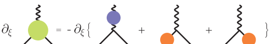
Figure 4.1: Pictorial representation of the on-shell Nielsen identity given by Eq.(4.72). The blobs in the lhs. represent bare one-loop contributions to the on-shell vertex and the blobs in the rhs. wfr. counter terms.

Replacing Eq. (4.71) in Eq. (4.56) we obtain

$$\partial_{\xi}\left(\bar{u}_{u}\left(p_{i}\right)\epsilon^{\mu}\left(q\right)\Gamma_{W_{\mu}^{+}\bar{u}_{i}d_{j}}^{\left(1\right)}v_{d}\left(-p_{j}\right)\right)$$ (4.72)

$$= \frac{e}{2s_{W}}M_{L}^{\left(1\right)}\partial_{\xi}\left(\delta\bar{Z}_{ir}^{uL}K_{rj}+K_{ir}\delta Z_{rj}^{dL}+\delta Z_{W}K_{ij}\right)$$

$$= -\frac{e}{2s_{W}}\partial_{\xi}\left(M_{L}^{\left(1\right)}\delta F_{L}^{\left(1\right)}+M_{L}^{\left(2\right)}\delta F_{L}^{\left(2\right)}+M_{R}^{\left(1\right)}\delta F_{R}^{\left(1\right)}+M_{R}^{\left(2\right)}\delta F_{R}^{\left(2\right)}\right)\,,$$

where Eq. (4.44) and the gauge independence of the electric charge and Weinberg angle has been used in the last equality. In the previous expression $M_{L,R}^{\left(i\right)}$ are understood with the physical momenta $p_{1}$ and $p_{2}$ of Eq. (4.42) replaced by the diagrammatic momenta $p_{i}$ and $-p_{j}$ respectively. Note that Eq. (4.72) states that the gauge dependence of the on-shell bare one-loop vertex function cancels out the renormalization counter terms appearing in Eq. (4.44) (see Fig. 4.1). This is one of the crucial results and special care should be taken not to ignore any of the absorptive parts —including those in the wfr. constants. As a consequence

$$\partial_{\xi}\mathcal{M}_{1}=-\frac{e}{2s_{W}}M_{L}^{\left(1\right)}\partial_{\xi}\delta K_{ij}\,,$$

and asking for a gauge independent amplitude the counter term for $K_{ij}$ must be separately gauge independent, as originally derived in [15].

Finally, since each structure $M_{L,R}^{\left(i\right)}$ must cancel separately we have that the Nielsen identities enforce

$$\partial_{\xi}\delta F_{L}^{\left(2\right)}=\partial_{\xi}\delta F_{R}^{\left(1\right)}=\partial_{\xi}\delta F_{R}^{\left(2\right)}=0\,.$$

8 Absorptive parts

Having determined in the previous section, thanks to an extensive use of the Nielsen identities, the gauge dependence of the different quantities appearing in top or $W$ decay in terms of the self-energies, we shall now proceed to list the absorptive parts of the wfr. constants, with special attention to their gauge dependence. The aim of this section is to state the differences between the wfr. constants given in our scheme and the ones in [19]. Recall that at one-loop such difference reduces to the absorptive ($\widetilde{Im}$) contribution to the $\delta Z$’s. In what concerns the gauge dependent part (with $\xi\geq 0$) the absorptive contribution ($\widetilde{Im}_{\xi}$) in the fermionic $\delta Z$’s amounts to

$$i\widetilde{Im}_{\xi}\left(\delta Z_{ij}^{uL}\right) = \sum_{h}\frac{iK_{ih}K_{hj}^{\dagger}}{8\pi v^{2}m_{j}^{u2}}\theta\left(m_{j}^{u}-m_{h}^{d}-\sqrt{\xi}M_{W}\right)\left(m_{j}^{u2}-m_{h}^{d2}-\xi M_{W}^{2}\right)$$

$$\times\sqrt{\left(\left(m_{j}^{u}-m_{h}^{d}\right)^{2}-\xi M_{W}^{2}\right)\left(\left(m_{j}^{u}+m_{h}^{d}\right)^{2}-\xi M_{W}^{2}\right)}\,,$$

$$i\widetilde{Im}_{\xi}\left(\delta\bar{Z}_{ij}^{uL}\right) = \sum_{h}\frac{iK_{ih}K_{hj}^{\dagger}}{8\pi v^{2}m_{i}^{u2}}\theta\left(m_{i}^{u}-m_{h}^{d}-\sqrt{\xi}M_{W}\right)\left(m_{i}^{u2}-m_{h}^{d2}-\xi M_{W}^{2}\right)$$

$$\times\sqrt{\left(\left(m_{i}^{u}-m_{h}^{d}\right)^{2}-\xi M_{W}^{2}\right)\left(\left(m_{i}^{u}+m_{h}^{d}\right)^{2}-\xi M_{W}^{2}\right)}\,,$$

$$\widetilde{Im}_{\xi}\left(\delta Z_{ij}^{uR}\right) = \widetilde{Im}_{\xi}\left(\delta\bar{Z}_{ij}^{uR}\right)=0\,,$$ (4.73)

where $\theta$ is the Heaviside function and $v$ is the Higgs vacuum expectation value (see appendix C). For the down $\delta Z$ we have the same formulae replacing $u\leftrightarrow d$ and $K\leftrightarrow K^{\dagger}.$ Note that the vanishing of $\widetilde{Im}_{\xi}\left(\delta Z_{ij}^{uR}\right)$ and $\widetilde{Im}_{\xi}\left(\delta\bar{Z}_{ij}^{uR}\right)$ could be anticipated from constraint (4.66) derived from Nielsen identities. Using these results we can write

$$i\partial_{\xi}\widetilde{Im}\left[\sum_{r}\left(\delta\bar{Z}_{ir}^{uL}K_{rj}+K_{ir}\delta Z_{rj}^{dL}\right)+\delta Z_{W}K_{ij}\right]$$ (4.74)

$$= K_{ij}\partial_{\xi}\left\{\frac{i}{8\pi v^{2}}\left[\frac{1}{m_{i}^{u2}}\theta\left(m_{i}^{u}-m_{j}^{d}-\sqrt{\xi}M_{W}\right)\left(m_{i}^{u2}-m_{j}^{d2}-\xi M_{W}^{2}\right)\right.\right.$$

$$+\left.\frac{1}{m_{j}^{d2}}\theta\left(m_{j}^{d}-m_{i}^{u}-\sqrt{\xi}M_{W}\right)\left(m_{j}^{d2}-m_{i}^{u2}-\xi M_{W}^{2}\right)\frac{{}}{{}}\right]$$

$$\times\left.\sqrt{\left(\left(m_{j}^{d}-m_{i}^{u}\right)^{2}-\xi M_{W}^{2}\right)\left(\left(m_{j}^{d}+m_{i}^{u}\right)^{2}-\xi M_{W}^{2}\right)}+i\widetilde{Im}_{\xi}\left(\delta Z_{W}\right)\frac{{}}{{}}\right\}\,.$$

In the case $\left|m_{i}^{u}-m_{j}^{d}\right|\leq\sqrt{\xi}M_{W}$ the above expression reduces to

$$\partial_{\xi}\sum_{r}\widetilde{Im}\left(\delta\bar{Z}_{ir}^{uL}K_{rj}+K_{ir}\delta Z_{rj}^{dL}\right)=0\,,$$ (4.75)

while for $\left|m_{i}^{u}-m_{j}^{d}\right|\geq\sqrt{\xi}M_{W}$ we have

$$i\partial_{\xi}\sum_{r}\widetilde{Im}\left(\delta\bar{Z}_{ir}^{uL}K_{rj}+K_{ir}\delta Z_{rj}^{dL}\right)$$ (4.76)

$$= K_{ij}\partial_{\xi}\left\{\frac{i}{4\pi v^{2}}\frac{\left|m_{i}^{u2}-m_{j}^{d2}\right|-\xi M_{W}^{2}}{m_{i}^{u2}+m_{j}^{d2}+\left|m_{i}^{u2}-m_{j}^{d2}\right|}\right.$$

$$\times\left.\sqrt{\left(\left(m_{j}^{d}-m_{i}^{u}\right)^{2}-\xi M_{W}^{2}\right)\left(\left(m_{j}^{d}+m_{i}^{u}\right)^{2}-\xi M_{W}^{2}\right)}\right\}\,.$$

Moreover the $\xi$-dependent absorptive contribution to $\delta Z_{W}$ ($\widetilde{Im}_{\xi}\left(\delta Z_{W}\right)$) has no dependence in quark masses since the diagram with a fermion loop is gauge independent. Because of that we can conclude that the derivative in Eq. (4.74) does not vanish. Defining $\Delta_{ij}$ as the difference between the vertex observable calculated in our scheme and the same in the scheme using $\widetilde{Re}$ we have

$$\Delta_{ij}\sim\left|K_{ij}\right|^{2}\mathrm{Re}\left(i\widetilde{Im}\delta Z_{W}\right)+\mathrm{Re}\left\{iK_{ij}^{\ast}\sum_{r}\left[\widetilde{Im}\left(\delta\bar{Z}_{ir}^{uL}\right)K_{rj}+K_{ir}\widetilde{Im}\left(\delta Z_{rj}^{dL}\right)\right]\right\}\,.$$

In the case of $\delta Z_{W}$ one can easily check that $\widetilde{Im}\left(\delta Z_{W}\right)=\mathrm{Im}\left(\delta Z_{W}\right)$ obtaining

$$\Delta_{ij}\sim\mathrm{Re}\left\{iK_{ij}^{\ast}\sum_{r}\left[\widetilde{Im}\left(\delta\bar{Z}_{ir}^{uL}\right)K_{rj}+K_{ir}\widetilde{Im}\left(\delta Z_{rj}^{dL}\right)\right]\right\}\,.$$ (4.77)

Thus from Eqs. (4.75), (4.76) and (4.77) we immediately obtain

$$\partial_{\xi}\Delta_{ij}\sim\mathrm{Re}\left\{iK_{ij}^{\ast}\sum_{r}\left[\partial_{\xi}\widetilde{Im}\left(\delta\bar{Z}_{ir}^{uL}\right)K_{rj}+K_{ir}\partial_{\xi}\widetilde{Im}\left(\delta Z_{rj}^{dL}\right)\right]\right\}=0\,.$$ (4.78)

However gauge independent absorptive parts, included if our prescription is used but not if one uses the one of [19] which makes use of the $\widetilde{Re}$, do contribute to Eq. (4.77). In order to see that we can take $\xi=1$ obtaining for the physical values of the masses

$$\widetilde{Im}_{\xi=1}\left(\delta Z_{rj}^{dL}\right) = 0\,,$$

$$\widetilde{Im}_{\xi=1}\left(\delta\bar{Z}_{ir}^{uL}\right) = \sum_{h}\frac{K_{ih}K_{hr}^{\dagger}}{8\pi v^{2}m_{i}^{u2}}\frac{\theta\left(m_{i}^{u}-m_{h}^{d}-M_{W}\right)}{m_{i}^{u2}-m_{r}^{u2}}$$

$$\times\sqrt{\left(m_{i}^{u2}-\left(M_{W}-m_{h}^{d}\right)^{2}\right)\left(m_{i}^{u2}-\left(M_{W}+m_{h}^{d}\right)^{2}\right)}$$

$$\times\left(\frac{1}{2}\left(m_{r}^{u2}+m_{h}^{d2}+2M_{W}^{2}\right)\left(m_{i}^{u2}+m_{h}^{2d}-M_{W}^{2}\right)-\left(m_{i}^{u2}+m_{r}^{u2}\right)m_{h}^{d2}\right)\,,$$

where only the results for $i\neq j$ have been presented. Note that $\widetilde{Im}_{\xi=1}\left(\delta\bar{Z}_{ir}^{uL}\right)\neq 0$ only when $i=3$, that is when the renormalized up-particle is a top. In addition, since the $m_{r}^{u2}$ dependence in Eq. (LABEL:zulb) does not vanish, CKM phases do not disappear from Eq. (4.77) and therefore

$$\Delta_{3j}\sim\mathrm{Re}\left\{iK_{3j}^{\ast}\sum_{r}\left[\widetilde{Im}\left(\delta\bar{Z}_{3r}^{uL}\right)K_{rj}+K_{3r}\widetilde{Im}\left(\delta Z_{rj}^{dL}\right)\right]\right\}\neq 0\,.$$ (4.80)

Eqs. (4.78) and (4.80) show that even though the difference $\Delta_{3j}$ is gauge independent, does not actually vanish. There are genuine gauge independent pieces that contribute not only to the amplitude, but also to the observable. As discussed these additional pieces cannot be absorbed by a redefinition of $K_{ij}$. Numerically such gauge independent corrections amounts roughly to $\Delta_{3j}\simeq 5\times 10^{-3}O_{\mathrm{tree}}$ where $O_{\mathrm{tree}}$ is the observable quantity calculated at leading order.

9 $CP$ violation and $CPT$ invariance

In this section we want to show that using wfr. constants that do not verify a pseudo-hermiticity condition does not lead to any unwanted pathologies. In particular: (a) No new sources of $CP$ violation appear besides the ones already present in the SM. (b) The total width of particles and anti-particles coincide, thus verifying the $CPT$ theorem. Let us start with the latter, which is not completely obvious since not all external particles and anti-particles are renormalized with the same constant due to the different absorptive parts.

The optical theorem asserts that

$$\Gamma_{t}\sim\sum_{f}\int d\Pi_{f}\left|M\left(t^{\left(\hat{n}\right)}\left(p\right)\rightarrow f\right)\right|^{2} = 2\mathrm{Im}\left[M\left(t^{\left(\hat{n}\right)}\left(p\right)\rightarrow t^{\left(\hat{n}\right)}\left(p\right)\right)\right]\,,$$ (4.81)

$$\Gamma_{\bar{t}}\sim\sum_{f}\int d\Pi_{f}\left|M\left(\bar{t}^{\left(\hat{n}\right)}\left(p\right)\rightarrow f\right)\right|^{2} = 2\mathrm{Im}\left[M\left(\bar{t}^{\left(\hat{n}\right)}\left(p\right)\rightarrow\bar{t}^{\left(\hat{n}\right)}\left(p\right)\right)\right]\,,$$ (4.82)

where we have consider, just as an example, top ($t^{\left(\hat{n}\right)}\left(p\right)$) and anti-top ($\bar{t}^{\left(\hat{n}\right)}\left(p\right)$) decay, with $p$ and $\hat{n}$ being their momentum and polarization. Recalling that the incoming fermion and outgoing anti-fermion spinors are renormalized with a common constant (see Eq. (4.1)) as are the outgoing fermion and incoming anti-fermion ones, it is immediate to see that

$$M\left(t^{\left(\hat{n}\right)}\left(p\right)\rightarrow t^{\left(\hat{n}\right)}\left(p\right)\right) = \bar{u}^{\left(\hat{n}\right)}\left(p\right)A_{33}\left(p\right)u^{\left(\hat{n}\right)}\left(p\right)\,,$$

$$M\left(\bar{t}^{\left(\hat{n}\right)}\left(p\right)\rightarrow\bar{t}^{\left(\hat{n}\right)}\left(p\right)\right) = -\bar{v}^{\left(\hat{n}\right)}\left(p\right)A_{33}\left(-p\right)v^{\left(\hat{n}\right)}\left(p\right)\,,$$

where the minus sign comes from an interchange of two fermion operators and where the subscripts in $A$ indicate family indices. Using the fact that

$$u^{\left(\hat{n}\right)}\left(p\right)\otimes\bar{u}^{\left(\hat{n}\right)}\left(p\right)=\frac{\not{p}+m}{2m}\frac{1+\gamma^{5}\not{n}}{2}\,,\qquad-v^{\left(\hat{n}\right)}\left(p\right)\otimes\bar{v}^{\left(\hat{n}\right)}\left(p\right)=\frac{-\not{p}+m}{2m}\frac{1+\gamma^{5}\not{n}}{2}\,,$$

with $n=\frac{1}{\sqrt{\left(p^{0}\right)^{2}-\left(\vec{p}\cdot\hat{n}\right)^{2}}}\left(\vec{p}\cdot\hat{n},p^{0}\hat{n}\right)$ being the polarization four-vector and performing some elementary manipulations we obtain

$$\bar{u}^{\left(\hat{n}\right)}\left(p\right)A_{33}\left(p\right)u^{\left(\hat{n}\right)}\left(p\right)$$

$$= Tr\left[\left(\frac{\not{p}+m}{2m}\frac{1+\gamma^{5}\not{n}}{2}\right)\left(a\left(p^{2}\right)\not{p}L+b\left(p^{2}\right)\not{p}R+c\left(p^{2}\right)L+d\left(p^{2}\right)R\right)\right]$$

$$= \frac{1}{4}Tr\left\{\frac{\not{p}+m}{2m}\left[\left(a\left(p^{2}\right)+b\left(p^{2}\right)\right)\not{p}+c\left(p^{2}\right)+d\left(p^{2}\right)\right]\right\}$$

$$= \frac{1}{4}Tr\left\{\frac{-\not{p}+m}{2m}\left[-\left(a\left(p^{2}\right)+b\left(p^{2}\right)\right)\not{p}+c\left(p^{2}\right)+d\left(p^{2}\right)\right]\right\}$$

$$= Tr\left[\frac{-\not{p}+m}{2m}\frac{1+\gamma^{5}\not{n}}{2}\left(-a\left(p^{2}\right)\not{p}L-b\left(p^{2}\right)\not{p}R+c\left(p^{2}\right)L+d\left(p^{2}\right)R\right)\right]$$

$$= -\bar{v}^{\left(\hat{n}\right)}\left(p\right)A_{33}\left(-p\right)v^{\left(\hat{n}\right)}\left(p\right)\,,$$

where we have decomposed $A_{33}\left(p\right)$ into its most general Dirac structure. We thus conclude the equality between Eqs. (4.81) and (4.82) verifying that the lifetimes of top and anti-top are identical. The detailed form of the wfr. constants, or whether they have absorptive parts or not, does not play any role.

Even thought total decay widths for top and anti-top are identical the partial ones need not to if $CP$ violation is present and some compensation between different processes must take place. Here we shall show that when $K=K^{\ast}$ the $CP$ invariance of the Lagrangian manifests itself in a zero asymmetry between the partial differential decay rate of top and its $CP$ conjugate process. The fact that the external renormalization constants have dispersive parts does not alter this conclusion. This is of course expected on rather general grounds, so the following discussion has to be taken really as a verification that no unexpected difficulties arise.

To illustrate this point let us consider the top decay channel $t\left(p_{1}\right)\rightarrow W^{+}\left(p_{1}-p_{2}\right)+b\left(p_{2}\right)$ and its $CP$ conjugate process $\bar{t}\left(\tilde{p}_{1}\right)\rightarrow W^{-}\left(\tilde{p}_{1}-\tilde{p}_{2}\right)+b\left(\tilde{p}_{2}\right).$ Let us note the respective amplitudes by $\mathcal{A}$ and $\mathcal{B}$ which are given as

$$\mathcal{A} = \varepsilon^{\mu}\bar{u}^{\left(s_{2}\right)}\left(p_{2}\right)A_{\mu}u^{\left(s_{1}\right)}\left(p_{1}\right)\,,$$

$$\mathcal{B} = -\tilde{\varepsilon}^{\mu}\bar{v}^{\left(s_{1}\right)}\left(\tilde{p}_{1}\right)B_{\mu}v^{\left(s_{2}\right)}\left(\tilde{p}_{2}\right)\,,$$

where $\tilde{a}^{\mu}=a_{\mu}=\left(a^{0},-a^{i}\right)$ for any four-vector. Considering contributions up to including next-to-leading corrections we have

$$A_{\mu} = -i\frac{e}{\sqrt{2}s_{W}}\left[\left(\bar{Z}^{\frac{1}{2}bL}K^{\dagger}Z^{\frac{1}{2}tL}+K^{\dagger}\delta_{V}+\delta K^{\dagger}\right)\gamma_{\mu}L+\delta F_{\mu}\right]\,,$$

$$B_{\mu} = -i\frac{e}{\sqrt{2}s_{W}}\left[\left(\bar{Z}^{\frac{1}{2}tL}KZ^{\frac{1}{2}bL}+K\delta_{V}+\delta K\right)\gamma_{\mu}L+\delta G_{\mu}\right]\,,$$

with $\delta_{V}$ $=\frac{\delta e}{e}-\frac{\delta s_{W}}{s_{W}}+\frac{1}{2}\delta Z_{W}$ and $\delta F_{\mu}$ and $\delta G_{\mu}$ are given by the one-loop diagrams. From a direct computation it can be seen that if $K=K^{\ast}$ this implies

$$\bar{Z}^{\frac{1}{2}L}=\left(Z^{\frac{1}{2}L}\right)^{T}\,,\quad\bar{Z}^{\frac{1}{2}R}=\left(Z^{\frac{1}{2}R}\right)^{T}\,,\quad\tilde{\varepsilon}^{\mu}\delta G_{\mu}=\varepsilon^{\mu}\gamma^{2}\delta F_{\mu}^{T}\gamma^{2}\,,$$ (4.83)

where the superscript $T$ means transposition with respect to all indices (family indices in the case of $Z^{\frac{1}{2}L}$ and $Z^{\frac{1}{2}R}$ and Dirac indices in the case of $\delta F_{\mu}$ ). Using

$$i\gamma^{2}\bar{u}^{\left(s\right)T}\left(p\right)=sv^{\left(s\right)}\left(\tilde{p}\right)\,,\qquad u^{\left(s\right)T}\left(p\right)i\gamma^{2}=-s\bar{v}^{\left(s\right)}\left(\tilde{p}\right)\,,$$

where $s=\pm 1$, depending on the spin direction in the $\hat{z}$ axis, we obtain

$$\mathcal{A} = \frac{-ie}{\sqrt{2}s_{W}}\varepsilon^{\mu}\bar{u}^{\left(s_{2}\right)}\left(p_{2}\right)\left[\left(\bar{Z}^{\frac{1}{2}bL}K^{\dagger}Z^{\frac{1}{2}tL}+K^{\dagger}\delta_{V}+\delta K^{\dagger}\right)\gamma_{\mu}L+\delta F_{\mu}\right]u^{\left(s_{1}\right)}\left(p_{1}\right)$$

$$= \frac{-ie}{\sqrt{2}s_{W}}\varepsilon^{\mu}u^{\left(s_{1}\right)T}\left(p_{1}\right)\left[L\left(\left(Z^{\frac{1}{2}tL}\right)^{T}K^{\ast}\left(\bar{Z}^{\frac{1}{2}bL}\right)^{T}+K^{\ast}\delta_{V}+\delta K^{\ast}\right)\gamma_{\mu}^{T}+\delta F_{\mu}^{T}\right]\bar{u}^{\left(s_{2}\right)T}\left(p_{2}\right)$$

$$= \frac{-s_{1}s_{2}ie}{\sqrt{2}s_{W}}\varepsilon^{\mu}\bar{v}^{\left(s_{1}\right)}\left(\tilde{p}_{1}\right)\gamma^{2}\left[L\left(\left(Z^{\frac{1}{2}tL}\right)^{T}K^{\ast}\left(\bar{Z}^{\frac{1}{2}bL}\right)^{T}+K^{\ast}\delta_{V}+\delta K^{\ast}\right)\gamma_{\mu}^{T}+\delta F_{\mu}^{T}\right]\gamma^{2}v^{\left(s_{2}\right)}\left(\tilde{p}_{2}\right)$$

$$= \frac{-s_{1}s_{2}ie}{\sqrt{2}s_{W}}\varepsilon^{\mu}\bar{v}^{\left(s_{1}\right)}\left(\tilde{p}_{1}\right)\left[\left(\left(Z^{\frac{1}{2}tL}\right)^{T}K^{\ast}\left(\bar{Z}^{\frac{1}{2}bL}\right)^{T}+K^{\ast}\delta_{V}+\delta K^{\ast}\right)\gamma_{\mu}^{\dagger}L+\gamma^{2}\delta F_{\mu}^{T}\gamma^{2}\right]v^{\left(s_{2}\right)}\left(\tilde{p}_{2}\right),$$

now using Eq. (4.83) we see that if no $CP$ violating phases are present in the CKM matrix $K$ (and therefore neither in $\delta K,$ Eq. (4.45)) we obtain that $\mathcal{A}=-s_{1}s_{2}\mathcal{B}$ and thus

$$\left|\mathcal{A}\right|^{2}=\left|\mathcal{B}\right|^{2}\,.$$

Note again that when $CP$ violating phases are present we can expect in general non-vanishing phase-space dependent asymmetries for the different channels. Once we sum over all channels and integrate over the final state phase space a compensation must take place as we have seen guaranteed by unitarity and $CPT$ invariance. Using a set of wfr. constants with absorptive parts as advocated here (and required by gauge invariance) leads to different results than using the prescription originally advocated in [19], in particular using Eq. (4.80) for $K\neq K^{\ast}$ we expect $\Delta_{3j}^{\left(t~{}decay\right)}-\Delta_{3j}^{\left(\bar{t}~{}decay\right)}\neq 0$.

10 Conclusions

Let us recapitulate the main results of this chapter. We hope, first of all, to have convinced the reader that there is a problem with what appears to be the commonly accepted prescription for dealing with wave function renormalization when mixing is present. The situation is even further complicated by the appearance of $CP$ violating phases. The problem has a twofold aspect. On the one hand the prescription of [19] does not diagonalize the propagator matrix in family space in what respects to the absorptive parts. On the other hand it yields gauge dependent amplitudes, albeit gauge independent modulus squared amplitudes. This is not satisfactory: interference with e.g. strong phases may reveal an unacceptable gauge dependence.

The only solution is to accept wfr. constants that do not satisfy a pseudo-hermiticity condition due to the presence of the absorptive parts, which are neglected in [19]. This immediately brings about some gauge independent absorptive parts which appear even in the modulus squared amplitude and which are neglected in the treatment of [19]. Furthermore, these parts (and the gauge dependent ones) cannot be absorbed in unitary redefinitions of the CKM matrix which are the only ones allowed by Ward identities. We have checked that —although unconventional— the presence of the absorptive parts in the wfr. constants is perfectly compatible with basic tenets of field theory and the Standard Model. Numerically we have found the differences to be important, at the order of the half per cent. Small, but relevant in the future. This information will be relevant to extract the experimental values of the CKM mixing matrix.

Traditionally, wave function renormalization seems to have been the “poor relative” in the Standard Model renormalization program. We have seen here that it is important on two counts. First because it is related to the counter terms for the CKM mixing matrix, although the on-shell values for wave function constants cannot be directly used there. Second because they are crucial to obtain gauge independent $S$ matrix elements and observables. While using our wfr. constants (but not the ones in [19]) for the external legs is strictly equivalent to considering reducible diagrams (with on-shell mass counter terms) the former procedure is considerably more practical.

Chapter 5 Probing LHC phenomenology: single top production

With the current limit on the Higgs mass already placed at 113.5 GeV [10] and no clear evidence for the existence of an elementary scalar (despite much controversy regarding the results of the last days of LEP) it makes sense to envisage an alternative to the minimal Standard Model described by an effective theory without any physical light scalar fields. This in spite of the seemingly good agreement between experiment and radiative corrections computed in the framework of the minimal Standard Model (see [11] however).

The four dimensional operators contributing to his effective theory were already analyzed in previous chapters. Here we plan to investigate some features that physics encoded in these operators introduce in the production of top (or anti-top) quarks at the LHC. In Chapter 2 we have discussed, among other things, some phenomenological consequences of this effective Lagrangian in the neutral current sector. Here we have chosen single top production because we are interested in probing the charged current sector.

In the electroweak sector tree level contribution to neutral and charged currents can be written as

$$-\frac{e}{4c_{W}s_{W}}\bar{f}\gamma^{\mu}\left(\kappa_{L}^{NC}L+\kappa_{R}^{NC}R\right)Z_{\mu}f-\frac{e}{s_{W}}\bar{f}\gamma^{\mu}\left(\kappa_{L}^{CC}L+\kappa_{R}^{CC}R\right)\frac{\tau^{-}}{2}W_{\mu}^{+}f+h.c.$$ (5.1)

The dominant process at LHC energies that tests $\kappa_{L}^{CC}$ and $\kappa_{R}^{CC}$ in a direct way (i.e. not through top decay) is single top production in the so-called $W-$gluon fusion channel. The electroweak subprocesses corresponding to this channel are depicted in Figs. (5.1) and (5.2), where light $u$-type quarks or $\bar{d}$-type antiquarks are extracted from the protons, respectively.

Figure 5.1: Feynman diagrams contributing single top production subprocess. In this case we have a $d$ as spectator quark

Figure 5.2: Feynman diagrams contributing single top production subprocess. In this case we have a $\bar{u}$ as spectator quark

Besides this dominant channel (250 pb at LHC [33]) single tops are also produced through the process where the $W^{+}$ boson interacts with a $b$-quark extracted from the sea of the proton (50 pb) and in the quark-quark fusion process (10 pb). This last process (s-channel) will be analyzed in the last chapter with top decay taken also into account.

In a proton-proton collision a bottom-anti-top pair is also produced through analogous subprocesses. The analysis of such anti-top production processes is similar to the top ones and the corresponding cross sections can be easily derived doing the appropriate changes (see appendix D).

In this chapter we will analyze the sensitivity of different LHC observables to the magnitude of charged current couplings $\kappa_{L}^{CC}$ and $\kappa_{R}^{CC}$ through single top production in the $W$-gluon fusion channel. In section 3 we show how the measurement of top spin plays a central role in the isolation of observables sensitive to left and right coupling variations. In this Chapter we do not analyze in detail top decay but we perform a theoretical approach at the issue of measuring top spin from its decay products. In this regard we show in section 4 that the presence of effective right-handed couplings implies that the top is not in a pure spin state, which is a fact that was overlooked in earlier works in the literature.

Moreover, in section 5 we show that there is a unique spin basis allowing the calculation of top production an decay convoluting the top decay products angular distribution with the polarized top differential cross section. In the next chapter we show explicitly this basis both for the t- and s- channels.

1 Effective couplings and observables

Including family mixing and, possibly, $CP$ violation, the complete set of dimension four effective operators which may contribute to the top effective couplings and are relevant for the present discussion is the set given by Eq. (3.6) [44, 68, 78]. In addition, as we have seen in Chapter 3 we have the ‘universal’ terms given by Eq. (3.3) which are present in the Standard Model. In Eq. (3.3) we allow for general couplings $X_{L}$, $X_{R}^{(u,d)}$; in the Standard Model these couplings can be renormalized away via a change of basis, but as we have seen Chapter 3 in more general theories they leave traces in other operators not present in the Standard Model [78].

In Chapter 3 we have also seen that when we diagonalize the mass matrix present in Eq. (3.3) via a redefinition of the matter fields $\left(\mathrm{f}\rightarrow f\right)$ we change also the structure of operators (3.6). Taking that into account, the contribution to the different gauge boson-fermion-fermion vertices is as follows

$$\mathcal{L}_{bff} = -g_{s}\bar{f}\gamma^{\mu}\left(a_{L}L+a_{R}R\right)\frac{\mathbf{\lambda}}{2}\mathbf{\cdot G}_{\mu}f,$$ (5.2)

$$-e\bar{f}\gamma^{\mu}\left(b_{L}L+b_{R}R\right)A_{\mu}f,$$

$$-\frac{e}{2c_{W}s_{W}}\bar{f}\gamma^{\mu}\left[\left(c_{L}^{u}\tau^{u}+c_{L}^{d}\tau^{d}\right)L+\left(c_{R}^{u}\tau^{u}+c_{R}^{d}\tau^{d}\right)R\right]Z_{\mu}f$$

$$-\frac{e}{s_{W}}\bar{f}\gamma^{\mu}\left[\left(d_{L}L+d_{R}R\right)\frac{\tau^{-}}{2}W_{\mu}^{+}+\left(d_{L}^{\dagger}L+d_{R}^{\dagger}R\right)\frac{\tau^{+}}{2}W_{\mu}^{-}\right]f,$$

where $\tau^{u}$ and $\tau^{d}$ are the up and down projectors and $f$ represents the matter fields in the physical, diagonal basis. It was shown in Chapter 3 that once the all the renormalization (vertex, CKM elements, wave-function) counterterms are taken into account we obtain $a_{L,R}=1$, $b_{L,R}=Q$; i.e. we have no contribution from the effective operators to the vertices of the gluon and photon. For the $Z$ couplings we get instead

$$c_{L}^{u} = 1-2Qs_{W}^{2}-\hat{M}_{L}^{1}-\hat{M}_{L}^{1\dagger}+\hat{M}_{L}^{2\dagger}+\hat{M}_{L}^{2}+\hat{M}_{L}^{3}+\hat{M}_{L}^{3\dagger},$$

$$c_{L}^{d} = -1-2Qs_{W}^{2}+K^{\dagger}\left(\hat{M}_{L}^{1}+\hat{M}_{L}^{1\dagger}+\hat{M}_{L}^{2\dagger}+\hat{M}_{L}^{2}-\hat{M}_{L}^{3}-\hat{M}_{L}^{3\dagger}\right)K,$$

$$c_{R}^{u} = -2s_{W}^{2}Q+\hat{M}_{R}^{1}+\hat{M}_{R}^{1\dagger}+\hat{M}_{R}^{2}+\hat{M}_{R}^{2\dagger}+\hat{M}_{R}^{3}+\hat{M}_{R}^{3\dagger},$$

$$c_{R}^{d} = -2s_{W}^{2}Q+\hat{M}_{R}^{1}+\hat{M}_{R}^{1\dagger}-\hat{M}_{R}^{2}-\hat{M}_{R}^{2\dagger}-\hat{M}_{R}^{3}-\hat{M}_{R}^{3\dagger},$$ (5.3)

where $K$ is the CKM matrix, and the matrices $\hat{M}_{L}$’s and $\hat{M}_{R}$’s are redefined matrices according to the results of Chapter 3 (the exact relation of these matrices to the $M_{L,R}^{i}$ of Eqs. (3.6) has no relevance for the present discussion). Finally for the charged couplings we have

$$d_{L} = K+\left(-\hat{M}_{L}^{1}-\hat{M}_{L}^{1\dagger}+\hat{M}_{L}^{2}-\hat{M}_{L}^{2\dagger}-\hat{M}_{L}^{3}-\hat{M}_{L}^{3\dagger}+\hat{M}_{L}^{4}-\hat{M}_{L}^{4\dagger}\right)K,$$

$$d_{R} = \hat{M}_{R}^{1}+\hat{M}_{R}^{1\dagger}+\hat{M}_{R}^{2}-\hat{M}_{R}^{2\dagger}-\hat{M}_{R}^{3}-\hat{M}_{R}^{3\dagger}.$$ (5.4)

Since the set of operators (3.6) is the most general one allowed by general requirements of gauge invariance, locality and hermiticity; it is clear that radiative corrections, when expanded in powers of $p^{2}$, can be incorporated into them. In fact, such an approach has proven to be very fruitful in the past. Once everything is included we are allowed to identify the couplings $d_{L,R}$ with $\kappa_{LR}^{CC}$. In this work we shall be concerned with the bounds that the LHC experiments will be able to set on the couplings $\kappa_{LR}^{CC}$, more specifically on the entries $tj$ of these matrices (those involving the top). In the rest of the chapter we do not consider mixing and we consider non-tree level and new physics contributions only on the $tb$ effective couplings, therefore in the numerical simulations we have taken

$$d_{L} = diag\ (K_{ud},K_{cs},g_{L}),$$

$$d_{R} = diag\ (0,0,g_{R}).$$

When we talk along this chapter about the results for the Standard Model at tree level we mean $g_{L}=1$, and $g_{R}=0$. However, even though numerical results are presented considering only the $tb$ entry ($g_{L}$ and $g_{R}$), since flavor indices and masses are kept all along in the analytical expressions (see appendix D), the appropriate changes to include other entries are immediate.

As we have seen in Chapter 2 the effective couplings of the neutral sector (5.3) can be determined from the $Z\rightarrow f~{}\bar{f}$ vertex [68], but at present not much is known from the $tb$ effective coupling. This is perhaps best evidenced by the fact that the current experimental results for the (left-handed) $K_{tb}$ matrix element give [84]

$$\frac{|K_{tb}|^{2}}{|K_{td}|^{2}+|K_{ts}|^{2}+|K_{tb}|^{2}}=0.99\pm 0.29.$$ (5.5)

In the Standard Model this matrix element is expected to be close to 1. It should be emphasized that these are the ‘measured’ or ‘effective’ values of the CKM matrix elements, and that they do not necessarily correspond, even in the Standard Model, to the entries of a unitary matrix on account of the presence of radiative corrections. These deviations with respect to unitary are expected to be small —at the few per cent level at most— unless new physics is present. At the Tevatron the left-handed couplings are expected to be eventually measured with a 5% accuracy [85]. The present work is a contribution to such an analysis in the case of the LHC experiments.

As far as experimental bounds for the right handed effective couplings is concerned, the more stringent ones come at present from the measurements on the $b\rightarrow s\gamma$ decay at CLEO [75]. Due to a $m_{t}/m_{b}$ enhancement of the chirality flipping contribution, a particular combination of mixing angles and $\kappa_{R}^{CC}$ can be found. The authors of [86] reach the conclusion that $|\mathrm{Re}(\kappa_{R}^{CC})|\leq 0.4\times 10^{-2}$. However, considering $\kappa_{R}^{CC}$ as a matrix in generation space, this bound only constraints the $tb$ element. Other effective couplings involving the top remain virtually unrestricted from the data. The previous bound on the right-handed coupling is a very stringent one. It is pretty obvious that the LHC will not be able to compete with such a bound. Yet, the measurement will be a direct one, not through loop corrections. Equally important is that it will yield information on the $td$ and $ts$ elements too, by just replacing the $\bar{b}$ quark in Figs. (5.1) and (5.2) by a $\bar{d}$ or a $\bar{s}$ respectively.

Now we shall proceed to analyze the bounds that single top production at the LHC can set on the effective couplings. This combined with the data from $Z$ physics will allow an estimation of the six effective couplings (5.3-5.4) in the matter sector of the effective electroweak Lagrangian. We will, in the present work limit ourselves to the consideration of the cross-sections for production of polarized top quarks. We shall not consider at this stage the potential of measuring top decays angular distributions in order to establish relevant bounds on the effective electroweak couplings. This issue merits a more detailed analysis, including the possibility of detecting $CP$ violation [87].

2 The cross section in the t-channel

In order to calculate the cross section $\sigma$ of the process $pp\rightarrow t\bar{b}$ we have used the CTEQ4 set of structure functions [88] to determine the probability of extracting a parton with a given fraction of momenta from the proton. Hence we write schematically

$$\sigma=\sum_{q}\int_{0}^{1}\int_{0}^{1}f_{g}(y)f_{q}(x)\hat{\sigma}(xP_{1},yP_{2})dxdy,$$ (5.6)

where $f_{q}$ denote the parton distribution function (PDF) corresponding to the partonic quarks and antiquarks and $f_{g}$ indicate the PDF corresponding to the gluon. In Eq.(5.6) we have set the light quark and gluon momenta to $xP_{1}$ and $yP_{1}$, respectively. ($P_{1}$ and $P_{2}$ are the four-momenta of the two colliding protons.) The approximation thus involves neglecting the transverse momenta of the incoming partons; the transverse fluctuations are integrated over by doing the appropriate integrals over $k_{T}$. We have then proceeded as follows. We have multiplied the parton distribution function of a gluon of a given momenta from the first proton by the sum of parton distribution functions for obtaining a $u$ type quark from the second proton. This result is then multiplied by the cross sections of the subprocesses of Fig. (5.1). We perform also the analogous process with the $\bar{d}$ type anti-quarks of Fig. (5.2). At the end, these two partial results are add up to obtain the total $pp\rightarrow t\bar{b}$ cross section.

Typically the top quark decays weakly well before strong interactions become relevant, we can in principle measure its polarization state with virtually no contamination of strong interactions (see e.g. [89] for discussions this point and section 5). For this reason we have considered polarized cross sections and provide general formulas for the production of polarized tops or anti-tops. To this end one needs to introduce the spin projector

$$\left(\frac{1+\gamma_{5}\not{n}}{2}\right),$$

with

$$n^{\mu} = \frac{1}{\sqrt{\left(p_{1}^{0}\right)^{2}-\left(\vec{p}_{1}\cdot\hat{n}\right)^{2}}}\left(\vec{p}_{1}\cdot\hat{n},p_{1}^{0}\hat{n}\right),$$ (5.7)

$$\hat{n}^{2} = 1,\qquad n^{2}=-1,$$

as the polarization projector for a particle or anti-particle of momentum $p_{1}$ with spin in the $\hat{n}$ direction. The calculation of the subprocesses cross sections have been performed for tops and anti-tops polarized in an arbitrary direction $\hat{n}$. Later we have analyzed numerically different spin frames defined as follows

• Lab helicity frame: the polarization vector is taken in the direction of the three momentum of the top or anti-top (right helicity) or in the opposite direction (left helicity).

• Lab spectator frame: the polarization vector is taken in the direction of the three momentum of the spectator quark jet or in the opposite direction. The spectator quark is the $d$-type quark in Fig. (5.1) or the $\bar{u}$-type quark in Fig. (5.2).

• Rest spectator frame: like in the Lab spectator frame we choose the spectator jet to define the polarization of the top or anti-top. Here, however, we define $\hat{n}$ as $\pm$ the direction of the three momentum of the spectator quark in the top or anti-top rest frame (given by a pure boost transformation $\Lambda$ of the lab frame). Then we have $n_{r}=\left(0,\hat{n}\right)$ in that frame and $n=\Lambda^{-1}n_{r}$ back to the lab frame.

The calculation of the subprocess polarized cross-section we present is completely analytical from beginning to end and the results are given in appendix.D Both the kinematics and the polarization vector of the top (or anti-top) are completely general. Since the calculation is of a certain complexity a number of checks have been done to ensure that no mistakes have been made. The integrated cross section agrees well with the results in [33] when the same cuts, scale, etc. are used. The mass of the top is obviously kept, but so is the bottom mass. The latter in fact turns out to be more relevant than expected as we shall see in a moment. As we have already discussed, the production of flavors other than ${\bar{b}}$ in association with the top can be easily derived from our results.

In single top production a distinction is often made between $2\rightarrow 2$ and $2\rightarrow 3$ processes. The latter corresponds, in fact, to the processes we have been discussing, the ones represented in Fig. (5.1), in which a gluon from the sea splits into a $b$ $\bar{b}$ pair. In the $2\rightarrow 2$ process the $b$ quark is assumed to be extracted from the sea of the proton, and both $b$ and $\bar{b}$ are collinear. Of course since the proton has no net $b$ content, a $\bar{b}$ quark must be present somewhere in the final state and the distinction between the two processes is purely kinematical. As is well known, when calculating the total cross section for single top production a logarithmic mass singularity [33] appears in the total cross section due to the collinear regime where the $b$ quark (and the $\bar{b}$) quark have $k_{T}\rightarrow 0$. This kinematic singularity is actually regulated by the mass of the bottom; it appears to all orders in perturbation theory and a proper treatment of this singularity requires the use of the Altarelli-Parisi equations and its resumation into a $b$ parton distribution function. While the evolution of the parton distribution functions is governed by perturbation theory, their initial values are not and some assumptions are unavoidable. Clearly an appropriate cut in $p_{T}$ should allow us to retain the perturbative regime of the $2\rightarrow 3$ process, while suppressing the $2\rightarrow 2$ one.

Two experimental approaches can be used at this point. One —advocated by Willenbrock and coworkers [33] is to focus on the low $p_{T}$ regime. The idea is to minimize the contribution of the $t,\bar{t}$ background, whose characteristic angular distributions are more central. Then one is actually interested in processes where one does not see the $\bar{b}$ (resp. $b$) quark which is produced in association with the $t$ quark (resp. $\bar{t}$), and accordingly sets an upper cut on the $p_{T}$ of the $\bar{b}$. Clearly one then has to take into account the $2\rightarrow 2$ process and, in particular, one must pay attention not to double count the low $p_{T}$ region (for the $\bar{b}$ (or $b$) quark) of the $2\rightarrow 3$ process, which is already included via a $b$ PDF and has to be subtracted. This strategy has some risks. First of all, the separation between the $2\rightarrow 3$ and $2\rightarrow 2$ is not a clear cut one. The separation takes place in a region where the cross section is rapidly varying so the results do depend to some extend on the way the separation is done. Also as we just said relies on some initial condition for the $b$ PDF at some initial scale (for instance at $\mu=m_{b}$. Moreover, this strategy does not completely avoid the background originated in $\bar{t}t$ production either; for instance when in the decaying $\bar{t}\rightarrow W^{-}\bar{b}\rightarrow\bar{u}d\bar{b}$ the $\bar{b}$ is missed along with the $\bar{u}$-type anti-quark in which case the $d$-type quark is taken as the spectator or when the $\bar{b}$ is missed along with the $d$-type quark in which case the $\bar{u}$-type anti-quark is taken as the spectator.

On the other hand, measuring the $\bar{b}$ (or $b$ for anti-top production) momenta will allow a better kinematic reconstruction of the individual processes. This should allow for a separation from the dominant mechanism of top production through gluon fusion. Setting a sufficiently high upper cut for the jet energy and a good jet separation might be sufficient to avoid contamination from $t,\bar{t}$ when one hadronic jet is missed. Finally, the spin structure of the top is completely different in both cases due to the chiral couplings in electroweak production. Therefore, according to this philosophy we have implemented a lower cut of 30 GeV in the transversal momentum of the $\bar{b}$ (resp. $b$) in top (resp. anti-top) production.

We do not really want to make strong claims as to which strategy should prove more efficient eventually. Many different ingredients have to be taken into account. Just to mention one more: the results of our analysis show that the sensitivity to the right handed effective coupling is not very big and that the (subdominant) s-channel process may actually be more adequate for this purpose. Yet, this is again more central, so one will need to consider the t-channel process for largish values of $p_{T}$ anyway.

3 A first look at the results

We shall now present the results of our analysis. To calculate the total event production corresponding to different observables we have used the integrating Monte Carlo program VEGAS [90]. We present results after one year (defined as 10⁷ seg.) run at full luminosity in one detector (100 $\mathrm{fb}^{-1}$ at LHC).

The total contribution to the electroweak vertices $g_{L}$, $g_{R}$ has two sources: the effective operators parametrizing new physics, and the contribution from the universal radiative corrections. In the standard model, neglecting mixing, for example, we have a tree level contribution to the $\bar{t}W_{\mu}^{+}b$ vertex given by $-\frac{i}{\sqrt{2}}\gamma_{\mu}gK_{tb}L$. Radiative corrections (universal and $M_{H}$ dependent) modify $g_{L}$ and generate a non zero $g_{R}$. These radiative corrections depend weakly on the energy of the process and thus in a first approximation we can take them as constant. Our purpose is to estimate the dependence of different LHC observables on these total effective couplings and how the experimental results can be used to set bounds on them. Assuming that the radiative corrections are known, this implies in turn a bound on the coefficients of the effective electroweak Lagrangian.

Figure 5.3: Anti-bottom transversal momentum distribution corresponding to unpolarized single top production at the LHC. The calculation was performed at the tree level in the Standard Model. Note the 30 GeV. cut implemented to avoid large logs due to the massless singularity in the total cross section. In this plot $\mu^{2}=\hat{s}=\left(q_{1}+q_{2}\right)^{2}$ too.

Let us start by discussing the experimental cuts. Due to geometrical detector constraints we cut off very low angles for the outgoing particles. The top, anti-bottom, and spectator quark have to come out with an angle in between 10 and 170 degrees. These angular cuts correspond to a cut in pseudorapidity $\left|\eta\right|<2.44$. In order to be able to detect the three jets corresponding to the outgoing particles we implements isolation cuts of 20 degrees between each other.

As already discussed we use a lower cut of 30 GeV in the $\bar{b}$ jet. This reduces the cross section to less than one third of its total value, since typically the $\bar{b}$ quark comes out in the same direction as the incoming gluon and a large fraction of them do not pass the cut (see Fig. (5.3)). Similarly, $p_{T}>20$ GeV cuts are set for the top and spectator quark jets. These cuts guarantee the validity of perturbation theory and will serve to separate from the overwhelming background of low $p_{T}$ physics. These values come as a compromise to preserve a good signal, while suppressing unwanted contributions. They are similar, but not identical to the ones used in [33] and [35]. To summarize the allowed regions are

$$\mathrm{detector~{}geometry~{}cuts} : 10^{o}\leq\theta_{i}\leq 170^{o},\quad i=t,\bar{b},q_{s},$$

$$\mathrm{isolation~{}cuts} : 20^{o}\leq\theta_{ij},\quad i,j=t,\bar{b},q_{s},$$

$$\mathrm{theoretical~{}cuts} : 20~{}\mathrm{GeV}\leq p_{1}^{T},\quad 20~{}\mathrm{GeV}\leq q_{2}^{T},\quad 30~{}\mathrm{GeV}\leq p_{2}^{T},$$ (5.8)

where $\theta_{t}$, $\theta_{\bar{b}},$ $\theta_{q_{s}}$ are the polar angles with respect to the beam line of the top, anti-bottom and spectator quark respectively; $\theta_{t\bar{b}}$, $\theta_{tq_{s}},$ $\theta_{\bar{b}q_{s}}$ are the angles between top and anti-bottom, top and spectator, and anti-bottom and spectator, respectively. The momenta conventions are given in Figs. (5.1) and (5.2).

Figure 5.4: Top transversal momentum distribution corresponding to polarized single top production at the LHC in the LAB system. The solid line corresponds to unpolarized top production and the dashed (dotted) line corresponds to tops of negative (positive) helicity. The subprocesses contributing to these histograms have been calculated at tree level in the electroweak theory. The cuts are described in the text. The degree of polarization in this spin basis and reference frame is only 69% . The QCD scale is taken to be $\mu^{2}=\hat{s}=\left(q_{1}+q_{2}\right)^{2}$.

Numerically, the dominant contribution to the process comes from the diagram where a $b$ quark is exchanged in the $t$ channel, but a large amount of cancellation takes place with the crossed interference term with the diagram with a top quark in the $t$ channel. The smallest contribution (but obviously non-negligible) corresponds to this last diagram. It is then easy to see, given the relative smallness of the $b$ mass, why the process is so much forward.

Undoubtedly the largest theoretical uncertainty in the whole calculation is the choice of a scale for $\alpha_{s}$ and the PDF’s. We perform a leading order calculation in QCD and the scale dependence is large. We have made two different choices. We present some results with the scale $p_{T}^{cut}$ used in $\alpha_{s}$ and the gluon PDF, while the virtuality of the $W$ boson is used as scale for the PDF of the light quarks in the proton. When we use these scales and compute, for instance, the total cross section above a cut of $p_{T}=20$ GeV in the $\bar{b}$ momentum, we get an excellent agreement with the calculations in [33]. Most of our results are however presented with a common scale $\mu^{2}=\hat{s}$, $\hat{s}$ being the center-of-mass energy squared of the $qg$ subprocess. The total cross section above the cut is then roughly speaking two thirds of the previous one, but no substantial change in the distributions takes place. It remains to be seen which one is the correct choice.

From our Monte Carlo simulation for single top production at the LHC after 1 year of full luminosity and with the cuts given above we obtain the total number of events. This number depends on the value of the effective couplings and on the top polarization vector $n$ given in the frames defined in section 2 . If we call $N\left(g_{L},g_{R},\hat{n},(frame)\right)$ to this quantity, we obtain the following results

$$N\left(g_{L},g_{R},\hat{n}=\pm\frac{\vec{p}_{1}}{\left|\vec{p}_{1}\right|},(lab)\right) = g_{L}^{2}\times\left(3.73\mp 1.31\right)\times 10^{5}+g_{R}^{2}\times\left(3.54\pm.97\right)\times 10^{5}$$

$$+g_{L}g_{R}\times\left(-.237\mp.0283\right)\times 10^{5},$$

$$N\left(g_{L},g_{R},\hat{n}=\pm\frac{\vec{q}_{2}}{\left|\vec{q}_{2}\right|},(lab)\right) = g_{L}^{2}\times\left(3.73\pm 2.22\right)\times 10^{5}+g_{R}^{2}\times\left(3.54\mp 2.12\right)\times 10^{5}$$

$$+g_{L}g_{R}\times\left(-.237\mp 0.001\right)\times 10^{5},$$

$$N\left(g_{L},g_{R},\hat{n}=\pm\frac{\vec{q}_{2}}{\left|\vec{q}_{2}\right|},(rest)\right) = g_{L}^{2}\times\left(3.73\pm 2.49\right)\times 10^{5}+g_{R}^{2}\times\left(3.54\mp 2.15\right)\times 10^{5}$$ (5.9)

$$+g_{L}g_{R}\times\left(-.237\mp.0180\right)\times 10^{5},$$

where we have omitted the $O\left(\sqrt{N}\right)$ statistical errors and we have neglected possible $CP$ phases ($g_{L}$ and $g_{R}$ real). One can observe from the simulations that the production of negative helicity (left) tops represents the 69% of the total single top production (see Fig. (5.4)), this predominance of left tops in the tree level electroweak approximation is expected due to the suppression at high energies of right-handed tops because of the zero right coupling in the charged current sector. In fact the production of right-handed tops would be zero were it not for the chirality flip, due to the top mass, in the t-channel. Of course the name ‘left’ and ‘right’ are a bit misleading; we really mean negative and positive helicity states.

Figure 5.5: Top transversal momentum distribution corresponding to polarized single top production at the LHC. The solid line corresponds to unpolarized top production and the dashed (dotted) line corresponds to tops polarized in the spectator jet negative (positive) direction in the top rest frame. In (a) the QCD scale is taken $\mu^{2}=\hat{s}=\left(q_{1}+q_{2}\right)^{2}$ and in (b) $\mu=p_{cut}^{T(bot)}=30$ GeV. The subprocesses contributing to these histograms have been calculated at tree level in the electroweak theory. With our set of cuts, the polarization is in both cases 84 %

Chirality states cannot be used, because the production is peaked in the 200 to 400 GeV region for the energy of the top and the mass cannot be neglected. The results for the production of tops polarized in the spectator jet direction in the top rest frame can be summarized in Fig. (5.5).

Figure 5.6: Anti-top transversal momentum distribution corresponding to polarized single anti-top production at the LHC. The solid line corresponds to unpolarized anti-top production and the dashed (dotted) line corresponds to anti-tops polarized in the spectator jet negative (positive) direction in the top rest frame. The subprocesses contributing to these histograms have been calculated at tree level in the electroweak theory, using the same cuts and conventions as in the previous figures.

We have also calculated single anti-top production obtaining a pattern similar to that of single top production but suppressed by an approximately 75% factor. This can be observed for example in Fig. (5.6). This suppression is generated by the parton distribution functions corresponding to negatively charged quarks that are smaller than the ones corresponding to positively charged quarks. Because of that the conclusions for anti-top production are practically the same as the ones for top production taking into account such suppression and that, because of the transformations (D.3) (see appendix D), passing from top to anti-top is equivalent to changing the spin direction.

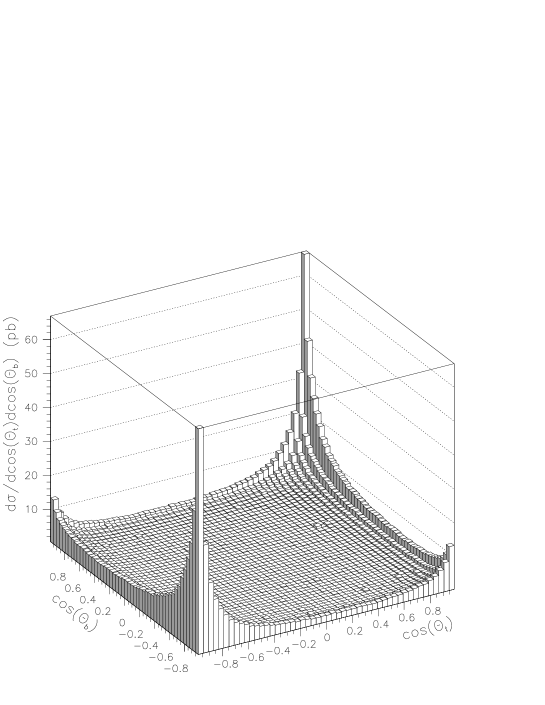
Figure 5.7: Distribution of the cosines of the polar angles of the top and anti-bottom with respect to the beam line. The plot corresponds to unpolarized single top production at the LHC. The calculation was performed at the tree level in Standard Model with $\mu^{2}=\hat{s}=\left(q_{1}+q_{2}\right)^{2}$.

Figure 5.8: Distribution of the cosine of the angle between top and anti-bottom corresponding to unpolarized single top production at the LHC. The calculation was performed at the tree level in Standard Model with $\mu^{2}=\hat{s}=\left(q_{1}+q_{2}\right)^{2}$. The abrupt fall near 1 is due to the 20 degrees isolation cut.

Figure 5.9: Distribution of the cosine of the angle between the spectator quark and the gluon corresponding to unpolarized single top production at the LHC. The momentum of the gluon is in the beam line direction but its sense is not observable so to obtain an observable distribution we have to symmetrize the above one. The calculation was performed at the tree level in Standard Model with $\mu^{2}=\hat{s}=\left(q_{1}+q_{2}\right)^{2}$.

In Fig. (5.7) we plot the cross section distribution of the polar angles of the top and anti-bottom with respect to the beam line for unpolarized single top production at the LHC. In Fig. (5.8) we plot the distribution of the cosine of the angle between the top and the anti-bottom for unpolarized single top production at the LHC. Everything is calculated in the (tree-level) Standard Model in the LAB frame. In both figures the above cuts are implemented, in particular the isolation cut of 20 degrees in the angle between the top and the anti-bottom is clearly visible in Fig. (5.8). In Fig. (5.9) we also present the distribution of the cosine of the angle between the spectator quark and the gluon. From inspection of these figures two facts emerge: a) the top-bottom distribution is strongly peaked in the beam direction as expected. b) Even with the presence of the isolation cut, near the beam axis configurations with top and anti-bottom almost parallel are flavored with respect to back-to-back configurations. Therefore this is an indication that almost back-to-back configurations are distributed more uniformly in space than parallel configurations favoring the beam line direction.

Figure 5.10: Top transversal momentum distribution corresponding to polarized single top production at the LHC. plots (a), (b) correspond to tops polarized in the spectator jet positive, negative direction respectively in the top rest frame. The subprocesses contributing to the solid line histogram have been calculated at tree level in the SM ($g_{L}=1$, $g_{R}=0$). The dashed (dotted) line histogram have been calculated at tree level with $g_{L}=1$, and $g_{R}=0.1$ ($g_{L}=1$, and $g_{R}=-0.1$). Note in (a) that the variation in the cross section due to the variation of the right coupling around its SM tree level value is practically inappreciable.

Let us now depart from the tree-level Standard Model and consider non-zero values for $\delta g_{L}$ and $\delta g_{R}$. In what concerns the dependence on the right effective coupling, our results are summarized in Fig. (5.10). From that figure it is quite apparent that negatively polarized tops (in the top rest frame, as previously described) are more sensitive to the value of the right coupling.

Taking into account the results of Eq. (5.9) we can establish the intervals where the effective couplings are indistinguishable from their tree level Standard Model values taking a 1 sigma deviation as a rough statistical criterion. Evidently we do not pretend to make here a serious experimental analysis since we are not taking into account the full set of experimental and theoretical uncertainties. Our aim is just to present an order of magnitude estimate of the sensitivity of the different spin basis to the value of the effective coupling around their tree level Standard Model value. The results are given in Table 5.1, where we indicate also the polarization vector chosen in each case. Of course those sensitivities (which, as said, are merely indicative) are calculated with the assumption that one could perfectly measure the top polarization in any of the above basis. As it is well known the top polarization is only measurable in an indirect way through the angular distribution of its decay products. In section 5 we outline the procedure to use our results to obtain a final angular distribution for the polarized top decay products (we believe that some confusion exists on this point). Obtaining that angular distribution involves a convolution of the single top production cross section with the decay products angular distribution and because of that we expect the true sensitivity to be worse than the ones given in Table 5.1. Obviously such distribution is an observable quantity and therefore must be independent of the spin basis one uses at an intermediate step calculation (in other words, the results must be independent of the basis in which the top spin density matrix is written). Because of that the discussion as to which is the “best” basis for the top polarization is somewhat academic in our view (see Chapter 4). Any basis will do; if any, the natural basis is that one where the density matrix becomes diagonal, where production and decay factorize. This basis corresponds to none of the above. However it may still be useful to know that some basis are more sensitive to the effective couplings than others if one assumes (at least as a gedanken experiment) that the polarization of the top could be measured directly.

It is worth mentioning that the bottom mass, which appears in the cross section in crossed left-right terms, such as $m_{b}g_{L}g_{R}$, plays a crucial role in the actual determination of $g_{R}$. This is because from the $|\mathrm{Re}(\kappa_{R}^{CC})|\leq 0.4\times 10^{-2}$ bound [86] we expect $g_{L}g_{R}m_{b}>g_{R}^{2}m_{t}.$ Evidently for the $ts$ or $td$ couplings these terms are not expected to be so relevant.

polarization, frame	$g_{L}$	$g_{R}$
$\hat{n}=\pm\frac{\vec{p}_{1}}{\left|\vec{p}_{1}\right|},~{}lab$	$\left[0.\,9986,1.\,0014\right]\quad~{}~{}\left(-\right)$	$\left[-0.26,0.85\right]\qquad~{}~{}~{}~{}\left(+\right)$
$\hat{n}=\pm\frac{\vec{q}_{2}}{\left|\vec{q}_{2}\right|},~{}lab$	$\left[0.9987,1.0013\right]\qquad\left(+\right)$	$\left[-0.013,0.063\right]\qquad\left(-\right)$
$\hat{n}=\pm\frac{\vec{q}_{2}}{\left|\vec{q}_{2}\right|},~{}rest$	$\left[0.9987,1.0013\right]\qquad\left(+\right)$	$\left[-0.021,0.059\right]\qquad\left(-\right)$

Table 5.1: Sensitivity of the polarized single top production to variations of the effective couplings. To calculate the intervals we have taken 2 sigma statistical deviations (95.5% confidence level) from tree level values as an order of magnitude criterion. Of course, given the uncertainties in the QCD scale, the overall normalization is dubious and the actual precision on $g_{L}$ a lot less. The purpose of these figures is to illustrate the relative accuracy. Between parenthesis we indicate the spin direction taken to calculate each interval.

4 The differential cross section for polarized tops

We define the matrix elements of the subprocess of Figs. (5.1) and (5.2) as $M_{+}^{d}$ and $M_{+}^{\bar{u}}$, respectively. We also define the matrix elements corresponding to the processes producing anti-tops as $M_{-}^{u}$, and $M_{-}^{\bar{d}}$. With these definitions the differential cross section for polarized tops $d\sigma$ can be written schematically as

$$d\sigma=\beta\left(f_{u}\left|M_{+}^{d}\right|^{2}+f_{\bar{d}}\left|M_{+}^{\bar{u}}\right|^{2}\right),$$

where $f_{u}$ and $f_{\bar{d}}$ denote the parton distribution functions corresponding to extracting a $u$-type quark and a $\bar{d}$-type quark respectively and $\beta$ is a proportionality factor incorporating the kinematics. Now using our analytical results for the matrix elements given in appendix D along with Eq. (D.3) and symmetries (D.4) we obtain

$$d\sigma = \beta f_{u}\left[\left|g_{L}\right|^{2}\left(a+a_{n}\right)+\left|g_{R}\right|^{2}\left(b+b_{n}\right)+\frac{g_{R}^{\ast}g_{L}+g_{R}g_{L}^{\ast}}{2}\left(c+c_{n}\right)+i\frac{g_{L}^{\ast}g_{R}-g_{R}^{\ast}g_{L}}{2}d_{n}\right]$$ (5.13)

$$+\beta f_{\bar{d}}\left[\left|g_{R}\right|^{2}\left(a-a_{n}\right)+\left|g_{L}\right|^{2}\left(b-b_{n}\right)+\frac{g_{R}^{\ast}g_{L}+g_{R}g_{L}^{\ast}}{2}\left(c-c_{n}\right)-i\frac{g_{L}^{\ast}g_{R}-g_{R}^{\ast}g_{L}}{2}d_{n}\right]$$

$$= \left(\begin{array}[]{cc}g_{L}^{\ast}&g_{R}^{\ast}\end{array}\right)A\left(\begin{array}[]{c}g_{L}\\ g_{R}\end{array}\right),$$

where

$$A=\beta\left(\begin{array}[]{cc}f_{u}\left(a+a_{n}\right)+f_{\bar{d}}\left(b-b_{n}\right)&\frac{1}{2}f_{u}\left(c+c_{n}+id_{n}\right)+\frac{1}{2}f_{\bar{d}}\left(c-c_{n}-id_{n}\right)\\ \frac{1}{2}f_{u}\left(c+c_{n}-id_{n}\right)+\frac{1}{2}f_{\bar{d}}\left(c-c_{n}+id_{n}\right)&f_{u}\left(b+b_{n}\right)+f_{\bar{d}}\left(a-a_{n}\right)\end{array}\right),$$ (5.14)

and where $a,$ $b$, $c$, $a_{n}$, $b_{n}$, $c_{n}$ and $d_{n}$ are independent of the effective couplings $g_{R}$ and $g_{L}$ and the subscripts $n$ indicate linear dependence on the top spin four-vector $n.$. From Eq. (5.14) we observe that $A$ is an Hermitian matrix and therefore it is diagonalizable with real eigenvalues. Moreover, from the positivity of $d\sigma$ we immediately arrive at the constraints

$$\det A \geq 0,$$ (5.15)

$$TrA \geq 0,$$ (5.16)

that is

$$\left(f_{u}\left(a+a_{n}\right)+f_{\bar{d}}\left(b-b_{n}\right)\right)\left(f_{u}\left(b+b_{n}\right)+f_{\bar{d}}\left(a-a_{n}\right)\right)$$ (5.17)

$$\geq \frac{1}{4}\left(c^{2}\left(f_{u}+f_{\bar{d}}\right)^{2}+\left(c_{n}^{2}+d_{n}^{2}\right)\left(f_{u}-f_{\bar{d}}\right)^{2}+2cc_{n}\left(f_{u}^{2}-f_{\bar{d}}^{2}\right)\right),$$

and

$$\left(f_{u}+f_{\bar{d}}\right)\left(a+b\right)+\left(f_{u}-f_{\bar{d}}\right)\left(a_{n}+b_{n}\right)\geq 0.$$ (5.18)

Note that it is not possible to saturate both constraints for the same configuration because this would imply a vanishing $A$ which in turn would imply relations such as

$$\frac{a+b}{a_{n}+b_{n}}=\frac{f_{\bar{d}}-f_{u}}{f_{\bar{d}}+f_{u}}=\frac{a_{n}-b_{n}}{a-b},$$

which evidently do not hold. Moreover, since constraints (5.17) and (5.18) must be satisfied for any set of positive PDF’s we immediately obtain the bounds

$$ab+a_{n}b_{n}-\frac{1}{4}\left(c^{2}+c_{n}^{2}+d_{n}^{2}\right) \geq \left|a_{n}b+ab_{n}-\frac{1}{2}cc_{n}\right|$$

$$b^{2}+a^{2}-\left(b_{n}^{2}+a_{n}^{2}\right) \geq \frac{1}{2}\left(c^{2}-\left(c_{n}^{2}+d_{n}^{2}\right)\right).$$

In order to have a 100% polarized top we need a spin four-vector $n$ that saturates the constraint (5.15) (that is Eq.(5.17)) for each kinematical situation, that is we need $A\left(n\right)$ to have a zero eigenvalue which is equivalent to have a unitary matrix $C$ satisfying

$$C^{\dagger}AC=\mathrm{diag}\left(\lambda,0\right),$$

for some positive eigenvalue $\lambda$. In general such $n$ need not exist and, should it exist, is in any case independent of the effective couplings $g_{R}$ and $g_{L}$. Moreover, provided this $n$ exists there is only one solution (up to a global complex normalization factor $\alpha$) for the pair $\left(g_{R},g_{L}\right)$ to the equation $d\sigma=0,$ This solution is just

$$g_{L} = \alpha C_{12},$$

$$g_{R} = \alpha C_{22}.$$ (5.19)

Note that if one of the effective couplings vanishes we can take the other constant and arbitrary. However if both effective couplings are non-vanishing we would have a quotient $g_{R}/g_{L}$ that would depend in general on the kinematics. This is not possible so we can conclude that for a non-vanishing $g_{R}$ ( $g_{L}$ is evidently non-vanishing) it is not possible to have a pure spin state (or, else, only for fine tuned $g_{R}$ a 100% polarization is possible).

To illustrate these considerations let us give an example: in the unphysical situation where $m_{t}\rightarrow 0$ it can be shown that there exists two solutions to the saturated constraint (5.15), namely

$$m_{t}n^{\mu}\rightarrow\pm\left(\left|\vec{p}_{1}\right|,p_{1}^{0}\frac{\vec{p}_{1}}{\left|\vec{p}_{1}\right|}\right),$$ (5.20)

once we have found this result we plug it in the expression (5.19) and we find the solutions $\left(0,g_{L}\right)$ with $g_{L}$ arbitrary for the $+$ sign and $\left(g_{R},0\right)$ with $g_{R}$ arbitrary for the $-$ sign. That is, physically we have zero probability of producing a right handed top when we have only a left handed coupling and viceversa when we have only a right handed coupling. Note that in this case it is clear that having both effective couplings non-vanishing would imply the absence of 100 % polarization in any spin basis. This can be understood in general remembering that the top particle forms in general an entangled state with the other particles of the process. Since we are tracing over the unknown spin degrees of freedom and over the flavors of the spectator quark we do not expect in general to end up with a top in a pure polarized state; although this is not impossible as it is shown the in the last example.

In the physical situation where $m_{t}\neq 0$ (we use $m_{t}=175.6$ GeV and $m_{b}=5$ GeV in this work) we have found that a spin basis with relatively high polarization is the one with the spin $\hat{n}$ taken in the direction of the spectator quark in the top rest frame. This is in accordance to the results in [35]. In general the degree of polarization ($\frac{N_{+\hat{n}}}{N_{+\hat{n}}+N_{-\hat{n}}}$) depends not only on the spin frame but also on the particular cuts chosen. We have found that the lower cut for the transverse momentum of the bottom worsens the polarization degree but, in spite of that, from Eq.(5.9) we see that we have a 84% of polarization in the Standard Model ($g_{L}=1,$ $g_{R}=0$) that is much bigger than the 69% obtained with the helicity frame. The above results follow the general trend of those presented by Mahlon and Parke [35], but in general, their degree of polarization is higher. We understand that this is due to the different cuts (in particular for the transversal momentum of the bottom) along with the different set of PDF’s used in our simulations.

5 Measuring the top polarization from its decay products

A well know result in the tree level SM regarding the measure of the top polarization from its decay products is the formula that states the following: Given a top polarized in the $\hat{n}$ direction in its rest frame, the lepton $l^{+}$ produced in the decay of the top via the process

$$t\rightarrow b\left(W^{+}\rightarrow l^{+}\nu_{l}\right),$$ (5.21)

presents an angular distribution [91]

$$\sigma_{l}=\alpha\left(1+\cos\theta\right),$$ (5.22)

where $\alpha$ is a normalization factor and $\theta$ is the axial angle measured from the direction of $\hat{n}.$ What can we do when the top is in a mixed state with no 100% polarization in any direction? The first naive answer would be: With any axis $\hat{n}$ in the top rest frame the top will have a polarization $p_{+}$ (with $0\leq p_{+}\leq 1)$ in that direction and a polarization $p_{-}=1-p_{+}$ in the opposite direction so the angular distribution for the lepton is

$$\sigma_{l} = \alpha\left(p_{+}\left(1+\cos\theta\right)+p_{-}\left(1-\cos\theta\right)\right)$$ (5.23)

$$= \alpha\left(1+\left(p_{+}-p_{-}\right)\cos\theta\right)$$

$$= \alpha\left(1+\left(2p_{+}-1\right)\cos\theta\right).$$

The problem with formula (5.23) is that the angular distribution for the lepton depends on the arbitrary chosen axis $\hat{n}$ and this cannot be correct. The correct answer can be obtained by noting the following facts:

• Given an arbitrary chosen axis $\hat{n}$ in the rest frame and the associated spin basis to it $\left\{\left|+\hat{n}\right\rangle,\left|-\hat{n}\right\rangle\right\}$ the top spin state in given by a $2\times 2$ density matrix $\rho$

  $$\rho=\rho_{+}\left|+\hat{n}\right\rangle\left\langle+\hat{n}\right|+\rho_{-}\left|-\hat{n}\right\rangle\left\langle-\hat{n}\right|+b\left|+\hat{n}\right\rangle\left\langle-\hat{n}\right|+b^{\ast}\left|-\hat{n}\right\rangle\left\langle+\hat{n}\right|,$$ (5.24)

  which is in general not diagonal ($b\neq 0$) and whose coefficients depend on the rest of kinematical variables determining the differential cross section.

• From the calculation of the polarized cross section we only know the diagonal elements $\rho_{\pm}=p_{\pm}=\left|M\right|_{\pm\hat{n}}^{2}/\left(\left|M\right|_{+\hat{n}}^{2}+\left|M\right|_{-\hat{n}}^{2}\right).$

• Given $\rho$ in any orthogonal basis determined (up to phases) by $\hat{n}$ we can change to another basis that diagonalizes $\rho.$ Since the top is a spin $1/2$ particle, this basis will correspond to another direction $\hat{n}_{d}$.

• Once we have $\rho$ diagonalized then Eq.(5.23) is trivially correct with $p_{\pm}=\rho_{\pm}$ and now $\theta$ is unambiguously measured from the direction of $\hat{n}_{d}.$

From the above facts the first question that comes to our minds is if there exists a way to determine $\hat{n}_{d}$ without knowing the off-diagonal matrix elements of $\rho.$ The answer is yes. It is an easy exercise of elementary quantum mechanics that given a $2\times 2$ Hermitian matrix $\rho$ the eigenvector with largest (lowest) eigenvalue correspond to the unitary vector that maximizes (minimizes) the bilinear form $\left\langle v\right|\rho\left|v\right\rangle$ constrained to $\left\{\left|v\right\rangle,~{}\left\langle v|v\right\rangle=1\right\}$. Since an arbitrary normalized $\left|v\right\rangle$ can be written (up to phases) as $\left|+\hat{n}\right\rangle$ and in that case $\rho_{+}=p_{+}$ then the correct $\hat{n}_{d}$ entering in Eq.(5.23) is the one that maximizes the differential cross section $\left|M\right|_{\hat{n}}^{2}$ for each kinematical configuration. At the end, the correct angular distribution for the leptons is given by the cross section for polarized tops in this basis ($\hat{n}_{d}$) convoluted with formula (5.22) (or improvements of it [92]).

The above analysis was carried out in the Standard Model ($g_{R}=0$) but it is correct also for $g_{R}\neq 0$ using the complete formula for this case

$$\sigma_{l}=\alpha\left(1+\left(p_{+}-p_{-}\right)\cos\theta\left(1-\frac{1}{4}\left|g_{R}\right|^{2}h\left(\frac{M_{W}^{2}}{m_{t}^{2}}\right)\right)\right),$$ (5.25)

where $h\left(\frac{M_{W}^{2}}{m_{t}^{2}}\right)\simeq 0.566$ [91]. Formula (5.25) deserves some comments:

• First of all we remember that $\theta$ is the angle (in the top rest frame) between the $\hat{n}$ that maximizes the difference $\left(p_{+}-p_{-}\right)$ and the three momentum of the lepton.

• Taking into account the above comment and that $\left(p_{+}-p_{-}\right)$ depends on $g_{L}$ and $g_{R}$ we see that also $\theta$ depends on $g_{L}$ and $g_{R}$.

• From the computational point of view, formula (5.25) is not an explicit formula because involves a process of maximization for each kinematical configuration.

• In some works in the literature [35] formula (5.25) is presented for an arbitrary choice of the spin basis $\left\{\left|\pm\hat{n}\right\rangle\right\}$ in the top rest frame. This is incorrect because it does not take into account that, in general, the top spin density matrix is not diagonal.

• In a recent work [92] $O\left(\alpha_{s}\right)$ corrections are incorporated to the polarized top decay angular analysis. In this work the density matrix for the top spin is properly taken into account. To connect this work with ours we have to replace their polarization vector $\vec{P}$ by $P\hat{n}_{d}$ where the magnitude of the top polarization $P$ is just the spin asymmetry $\left(\left|M\right|_{+\hat{n}_{d}}^{2}-\left|M\right|_{-\hat{n}_{d}}^{2}\right)/\left(\left|M\right|_{+\hat{n}_{d}}^{2}+\left|M\right|_{-\hat{n}_{d}}^{2}\right)$ in our language. This taken into account, the density matrix the authors of [92] quote is in the basis $\left\{\left|+\hat{n}_{W^{+}}\right\rangle,\left|-\hat{n}_{W^{+}}\right\rangle\right\}$ where $\hat{n}_{W^{+}}$ is a normal vector in the direction of the three momentum of the $W^{+}$ (in the top rest frame).

6 Conclusions

We have done a complete calculation of the subprocess cross sections for polarized tops or anti-tops including the right effective coupling and bottom mass corrections. We have used a $p_{T}>30$ GeV cut in the transverse momentum of the produced $\bar{b}$ quark and, accordingly we have retained only the so called $2\rightarrow 3$ process, for the reasons described in the text.

Our analysis here is completely general. No approximation is made. We use the most general set of couplings and, since our approach is completely analytical, we can describe the contribution from other intermediate quarks in the $t$ channel, mixing, etc. Masses and mixing angles are retained. On the contrary, the analysis has to be considered only preliminary from an experimental point of view. No detailed study of the backgrounds has been made, except for the dominant $gg\rightarrow t\bar{t}$ process which has been considered to some extent (although again without quantitative evaluation).

Given the (presumed) smallness of the right handed couplings, the bottom mass plays a role which is more important than anticipated, as the mixed crossed $g_{L}g_{R}$ term, which actually is the most sensitive one to $g_{R}$ is accompanied by a $b$ quark mass. The statistical sensitivity to different values of this coupling is given in the text.

We present a variety of $p_{T}$ and angular distributions both for the $t$ and the $\bar{b}$ quarks. Obviously, the top decays shortly after production, but we have not made detailed simulations of this part. In fact, the interest of this decay is obvious: one can measure the spin of the top through the angular distribution of the leptons produced in this decay. In the Standard Model, single top production gives a high degree of polarization (84 % in the optimal basis, with the present set of cuts). This is a high degree of polarization, but well below the 90+ claimed by Mahlon and Parke in [35]. We understand this being due to the presence of the 30 GeV cut. In fact, if we remove this cut completely we get a 91 % polarization. Still below the result of [35] but in rough agreement (note that we do not include the $2\rightarrow 2$ process). Inasmuch as they can be compared our results are in good agreement with those presented in [33] in what concerns the total cross-section. Two different choices for the strong scale $\mu^{2}$ are presented.

In addition, it turns out that when $g_{R}\neq 0$ the top can never be 100% polarized. In other words, it is in a mixed state. In this case we show that a unique spin basis is singled out which allows one to connect top decay products angular distribution with the polarized top differential cross section.

Finally it should be mentioned that a previous study for this process in the present context was performed in [36] using the effective W approximation [93], in which the $W$ is treated as a parton of the proton. While this is certainly not an exact treatment, it was expected to be sufficiently good for our purposes. In the course of this work we have found, however, a number of differences.

Chapter 6 Single top production in the s-channel and top decay

In the previous chapter we have analyzed in detail the dominant t-channel mechanism of single top production and the sensitivity to values of the effective couplings $g_{L}$ and $g_{R}$ departing from their SM tree-level values.

As it has been discussed in Chapter 5, to be able to tell the corrections due to a right effective coupling from those due to a left one needs to measure the polarization of the top. Of course the top decays shortly after its production and all one can hope to see are the decay products. Since there is a correlation between the angular momentum of the top and the angular distribution of those products, one might hope to be able to ‘measure’ the top polarization and thus separate left from right contributions. Obviously, since the correlation is not a delta function (prohibited by quantum mechanics), some information must be lost along the top decay process.

Although the calculations in Chapter 5 were presented for the production of polarized tops, with respect to an arbitrary axis, and something was said there about the subsequent top decay, the issue was not discussed in great detail. In this chapter we would like to analyze this point more deeply. We shall not do so, however, in the t-channel process, but rather in the much simpler s-channel production mechanism. Although this mechanism is subleading (see the discussion in the previous chapter concerning the different contributions to the cross section for single top production) it is not negligible at all. Furthermore, the results obtained here can be carried over to the t-channel process without much difficulty.

In this chapter we will thus complete some of the more subtle aspects of single top production that were not taken into account in last chapter. The process analyzed in this chapter is given by Fig. (6.1).

Figure 6.1: Feynman diagram contributing to single top production and decay process in the s-channel.

Here, exactly as we did in Chapter 5, we shall assume that the produced top is on-shell, namely we study the production and subsequent decay of real tops. This way of proceeding goes under the name of narrow width approximation and it is a standard practice to analyze complicated processes consisting on the production of an unstable particle followed by its decay.

1 Cross sections for top production and decay

Using the momenta conventions of Fig. (6.1) and averaging over colors and spins of the initial fermions and summing over colors and spins of the final fermions (remember that we have included a spin projector for the top) the squared amplitude for top production is given by

$$\left|M_{n}\right|^{2} = \frac{e^{4}N_{c}}{s_{W}^{4}}\left(\frac{1}{k^{2}-M_{W}^{2}}\right)^{2}$$ (6.1)

$$\times\left\{\left|\tilde{g}_{L}\right|^{2}\left[\left|g_{R}\right|^{2}\left(q_{1}\cdot\frac{p_{1}+m_{t}n}{2}\right)\left(q_{2}\cdot\tilde{p}_{2}\right)+\left|g_{L}\right|^{2}\left(q_{2}\cdot\frac{p_{1}-m_{t}n}{2}\right)\left(q_{1}\cdot\tilde{p}_{2}\right)\right.\right.$$

$$+m_{b}\frac{g_{L}g_{R}^{\ast}+g_{R}g_{L}^{\ast}}{4}\left[m_{t}\left(q_{1}\cdot q_{2}\right)+\left(q_{2}\cdot p_{1}\right)\left(q_{1}\cdot n\right)-\left(q_{2}\cdot n\right)\left(q_{1}\cdot p_{1}\right)\right]$$

$$+\left.\left.im_{b}\frac{g_{L}g_{R}^{\ast}-g_{R}g_{L}^{\ast}}{4}\varepsilon_{\mu\alpha\rho\sigma}n^{\mu}p_{1}^{\alpha}q_{1}^{\rho}q_{2}^{\sigma}\right]\right\}$$

$$+\left|\tilde{g}_{R}\right|^{2}\left[\left|g_{R}\right|^{2}\left(q_{2}\cdot\frac{p_{1}+m_{t}n}{2}\right)\left(q_{1}\cdot\tilde{p}_{2}\right)+\left|g_{L}\right|^{2}\left(q_{1}\cdot\frac{p_{1}-m_{t}n}{2}\right)\left(q_{2}\cdot\tilde{p}_{2}\right)\right.$$

$$+m_{b}\frac{g_{L}g_{R}^{\ast}+g_{R}g_{L}^{\ast}}{4}\left[m_{t}\left(q_{1}\cdot q_{2}\right)+\left(q_{1}\cdot p_{1}\right)\left(q_{2}\cdot n\right)-\left(q_{1}\cdot n\right)\left(q_{2}\cdot p_{1}\right)\right]$$

$$+\left.\left.im_{b}\frac{g_{L}g_{R}^{\ast}-g_{R}g_{L}^{\ast}}{4}\varepsilon_{\mu\alpha\rho\sigma}n^{\mu}p_{1}^{\alpha}q_{2}^{\rho}q_{1}^{\sigma}\right]\right\},$$

where $\tilde{g}_{L},$ and $\tilde{g}_{R}$ are left and right couplings to the light quarks and $g_{L}$ and $g_{R}$ the coupling to the heavy up bottom system. In the simulations we have taken $\tilde{g}_{L}=1,$ $\tilde{g}_{R}=0.$ Hence the differential cross section for producing polarized tops is given by

$$d\sigma_{\hat{n}} = f\left(\tilde{x}_{1},\tilde{x}_{2},\left(q_{1}+q_{2}\right)^{2},\Lambda_{QCD}\right)d\tilde{x}_{1}d\tilde{x}_{2}\frac{1}{4\left|q_{2}^{0}\overrightarrow{q_{1}}-\overrightarrow{q_{2}}q_{1}^{0}\right|}$$

$$\times\frac{d^{3}p_{1}}{\left(2\pi\right)^{3}2p_{1}^{0}}\frac{d^{3}\tilde{p}_{2}}{\left(2\pi\right)^{3}2\tilde{p}_{2}^{0}}\left|M_{n}\right|^{2}\left(2\pi\right)^{4}\delta^{4}\left(q_{1}+q_{2}-p_{1}-p_{2}\right)$$

where $f\left(\tilde{x}_{1},\tilde{x}_{2},\left(q_{1}+q_{2}\right)^{2},\Lambda_{QCD}\right)d\tilde{x}_{1}d\tilde{x}_{2}$ accounts for the PDF contribution. For the top the total decay rate is given by

$$\Gamma = \frac{e^{2}}{s_{W}^{2}}\left\{\left(\left|g_{L}\right|^{2}+\left|g_{R}\right|^{2}\right)\left(m_{t}^{2}+m_{b}^{2}-2M_{W}^{2}+\frac{\left(m_{t}^{2}-m_{b}^{2}\right)^{2}}{M_{W}^{2}}\right)\right.$$

$$\left.-12m_{t}m_{b}\frac{g_{L}g_{R}^{\ast}+g_{R}g_{L}^{\ast}}{2}\right\}\frac{\sqrt{\left(m_{t}^{2}+m_{b}^{2}-M_{W}^{2}\right)^{2}-4m_{t}^{2}m_{b}^{2}}}{64\pi m_{t}^{2}p_{1}^{0}}.$$

The squared amplitude corresponding to the decay rate in the channel depicted in Fig. (6.1) summing over the top polarizations (with a spin projector inserted), averaging over its colors and summing over colors and polarizations of decay products is given by

$$\left|M_{n}^{D}\right|^{2}=\frac{-4}{N_{c}}\left|M_{n}\right|^{2}\left(q_{1}\rightarrow k_{2},\ q_{2}\rightarrow k_{1},\ \tilde{p}_{2}\rightarrow-p_{2}\right),$$

where $\left|M_{n}\right|^{2}\left(q_{1}\rightarrow k_{2},\ q_{2}\rightarrow k_{1},\ \tilde{p}_{2}\rightarrow-p_{2}\right)$ is just expression (6.1) with the indicated changes in momenta Now $\tilde{g}_{L},$ and $\tilde{g}_{R}$ are left and right couplings corresponding to the lepton-neutrino vertex and we have taken again $\tilde{g}_{L}=1,$ $\tilde{g}_{R}=0.$ Hence the decay rate differential cross section for this channel is given by

$$d\Gamma_{n}=\frac{\left|M_{n}^{D}\right|^{2}}{2p_{1}^{0}}\frac{d^{3}k_{1}}{\left(2\pi\right)^{3}2k_{2}^{0}}\frac{d^{3}k_{2}}{\left(2\pi\right)^{3}2k_{1}^{0}}\frac{d^{3}p_{2}}{\left(2\pi\right)^{3}2p_{2}^{0}}\left(2\pi\right)^{4}\delta^{4}\left(k_{1}+k_{2}+p_{2}-p_{1}\right).$$

Using the narrow-width approximation we have that the differential cross section $d\sigma$ corresponding to Fig. (6.1) is given by

$$d\sigma=\sum_{\pm n}d\sigma_{n}\times\frac{d\Gamma_{n}}{\Gamma}.$$ (6.2)

2 The role of spin in the narrow-width approximation

Within the narrow-width approximation we decompose the process depicted in Fig. (6.1) in two consecutive processes, the top production and its consecutive decay. In that set up we denote the single top production amplitude as $A_{p,\pm\hat{n}\left(p\right)}$ and the top decay amplitude as $B_{p,\pm\hat{n}\left(p\right)}.$ In the polar representation we write

$$A_{p,\pm\hat{n}\left(p\right)} = \left|A_{p,\pm\hat{n}\left(p\right)}\right|e^{i\varphi_{\pm}\left(p\right)},$$

$$B_{p,\pm\hat{n}\left(p\right)} = \left|B_{p,\pm\hat{n}\left(p\right)}\right|e^{i\omega_{\pm}\left(p\right)},$$

where $p$ indicate external momenta and $\hat{n}\left(p\right)$ a given spin basis for the top (see section 2 in Chapter 5). The differential cross section for the whole process $\mathcal{M}$ is schematically given by

$$d\mathcal{\sigma}=\int\left|A_{p,+\hat{n}\left(p\right)}B_{p,+\hat{n}\left(p\right)}+A_{p,-\hat{n}\left(p\right)}B_{p,-\hat{n}\left(p\right)}\right|^{2}dp,$$ (6.3)

where the integration over momenta is taken outside the modulus squared because these are unseen external momenta (like neutrino momenta, or angular and longitudinal momenta variables in $p_{T}$ histograms, etc.). Since there are still some kinematical variables still pending for integration (for example $p_{T}$ in $p_{T}$ distributions) we keep the “$d$”  in front of $\mathcal{\sigma}$. Hence

$$d\mathcal{\sigma} = \int\left|A_{p,+\hat{n}\left(p\right)}\right|^{2}\left|B_{p,+\hat{n}\left(p\right)}\right|^{2}dp+\int\left|A_{p,-\hat{n}\left(p\right)}\right|^{2}\left|B_{p,-\hat{n}\left(p\right)}\right|^{2}dp$$ (6.4)

$$+2\int\left|A_{p,+\hat{n}\left(p\right)}\right|\left|B_{p,+\hat{n}\left(p\right)}\right|\left|A_{p,-\hat{n}\left(p\right)}\right|\left|B_{p,-\hat{n}\left(p\right)}\right|$$

$$\times\cos\left(\varphi_{+}\left(p\right)-\varphi_{-}\left(p\right)+\omega_{+}\left(p\right)-\omega_{-}\left(p\right)\right)dp$$

$$\simeq \int\left|A_{p,+\hat{n}\left(p\right)}\right|^{2}\left|B_{p,+\hat{n}\left(p\right)}\right|^{2}dp+\int\left|A_{p,-\hat{n}\left(p\right)}\right|^{2}\left|B_{p,-\hat{n}\left(p\right)}\right|^{2}dp.$$

Since the axis with respect to which the spin basis is defined is completely arbitrary $d\mathcal{\sigma}$ is independent on this choice of basis. However within the narrow width approximation one does not compute $d\mathcal{\sigma}$ following formula (6.3). The practical procedure relies in computing the probability of producing a polarized top and then multiplying this probability by the probability of a given decay channel (see Eq. (6.2)). This procedure is equivalent to the neglection of the interference term in formula (6.4) as indicated there.

Let us see whether this approximation can justified. Clearly, the integration over momenta enhances the positive-definite terms in front of the interference oscillating one. If in addition we make a choice for $\hat{n}\left(p\right)$ that diagonalizes the top spin density matrix (see Chapter 5) and thus maximizes $\left|A_{p,+\hat{n}\left(p\right)}\right|$ and minimizes $\left|A_{p,-\hat{n}\left(p\right)}\right|$, then we expect the interference term to be negligible when compared to $\int\left|A_{p,+\hat{n}\left(p\right)}\right|^{2}\left|B_{p,+\hat{n}\left(p\right)}\right|^{2}dp$ even for small amount of phase space integration. In the s-channel we will see in the next section that the limit of $g_{R}\rightarrow 0$ there exists a spin basis $\hat{n}\left(p\right)$ where $\left|A_{p,-\hat{n}\left(p\right)}\right|$ is strictly zero. This basis is given by

$$n=\frac{1}{m_{t}}\left(\frac{m_{t}^{2}}{\left(q_{2}\cdot p_{1}\right)}q_{2}-p_{1}\right).$$

From this it follows that for small $g_{R}$ if we use that basis the interference integrand is already negligible with respect to the dominant term $\int\left|A_{p,+\hat{n}\left(p\right)}\right|^{2}\left|B_{p,+\hat{n}\left(p\right)}\right|^{2}dp$. For $g_{R}\neq 0$ one can still find a basis that maximizes $\left|A_{p,+\hat{n}\left(p\right)}\right|$ (and minimizes $\left|A_{p,-\hat{n}\left(p\right)}\right|$) and therefore diagonalizes the top density matrix $\rho$ (see section 5 in Chapter 5) In the next section we will show how to obtain such a basis that will be the one used in our numerical integration. In these simulations we have checked numerically that this basis is the one that maximizes $d\mathcal{\sigma}$ and therefore, on the same grounds, the one that minimizes the interference term.

Given that the observables are strictly independent of the choice of spin basis only if the interference term is included, we can easily assess the importance of the latter by checking to what extent a residual spin basis dependence is present. We have checked numerically this point by changing the definition of the spin basis $\hat{n}\left(p\right)$ and noting that our results are weakly dependent on the choice of $\hat{n}\left(p\right)$. A $3.8\%$ maximum variation was found between our diagonal basis and another orthogonal to the beam axis (that is, almost orthogonal to all momenta). Moreover we have checked that if spin is ignored altogether the same amount of variation is observed. Thus we conclude that even though the dependence on the choice of spin basis is not dramatic, its consideration is a must for a precise description using the narrow-width approximation.

3 The diagonal basis

As stated in the previous section in order to calculate the top decay we have to find the basis where the polarized single top production cross section is maximal. The can do this maximizing in the $4$-dimensional space generated by the components of $n$ constrained by

$$n\cdot p_{1}=0,\qquad n^{2}=-1,$$ (6.5)

where $p_{1}$ is the top four-moment, that is

$$n^{0} = \frac{n^{1}p_{1}^{1}+n^{2}p_{1}^{2}+n^{2}p_{1}^{2}}{p_{1}^{0}},$$

$$\left(p_{1}^{0}\right)^{2} = \left(p_{1}^{0}\right)^{2}\left\|\vec{n}\right\|^{2}-\left(n^{1}p_{1}^{1}+n^{2}p_{1}^{2}+n^{2}p_{1}^{2}\right)^{2},$$

where $\left\|\vec{n}\right\|=\sqrt{\left(n^{1}\right)^{2}+\left(n^{2}\right)^{2}+\left(n^{3}\right)^{2}}$, that is $n^{i}=\left\|\vec{n}\right\|\hat{n}^{i}$ with $\hat{n}$ the normalized spin three-vector. From above equations we obtain

$$\left\|\vec{n}\right\| = \frac{p_{1}^{0}}{\sqrt{\left(p_{1}^{0}\right)^{2}-\left(\hat{n}^{1}p_{1}^{1}+\hat{n}^{2}p_{1}^{2}+\hat{n}^{2}p_{1}^{2}\right)^{2}}},$$

$$n^{0} = \left\|\vec{n}\right\|\frac{\hat{n}^{1}p_{1}^{1}+\hat{n}^{2}p_{1}^{2}+\hat{n}^{2}p_{1}^{2}}{p_{1}^{0}},$$

from which Eq. (5.7) follows immediately. Let us now find the polarization vector that maximizes and minimizes the differential cross section of single top production.

3.1 The t-channel

We will begin with the t-channel the was analyzed in the previous chapter. Using Eq. (5.13) we define

$$a_{n} = n\cdot a,\qquad b_{n}=n\cdot b,$$

$$c_{n} = n\cdot c,\qquad d_{n}=n\cdot d,$$ (6.6)

and using Lagrange multipliers $\lambda_{1}$ and $\lambda_{2}$ for constraints (6.5) we maximize

$$\sigma+\lambda_{1}\left(n^{2}+1\right)+\lambda_{2}n\cdot p_{1},$$

obtaining the equations

$$n = -\frac{\beta}{2\lambda_{1}}f_{u}\left[\left|g_{L}\right|^{2}a+\left|g_{R}\right|^{2}b+\frac{g_{R}^{\ast}g_{L}+g_{R}g_{L}^{\ast}}{2}c+i\frac{g_{L}^{\ast}g_{R}-g_{R}^{\ast}g_{L}}{2}d\right]$$ (6.7)

$$+\frac{\beta}{2\lambda_{1}}f_{\bar{d}}\left[\left|g_{R}\right|^{2}a+\left|g_{L}\right|^{2}b+\frac{g_{R}^{\ast}g_{L}+g_{R}g_{L}^{\ast}}{2}c+i\frac{g_{L}^{\ast}g_{R}-g_{R}^{\ast}g_{L}}{2}d\right]-\frac{\lambda_{2}}{2\lambda_{1}}p_{1},$$

$$0 = n^{2}+1,$$ (6.8)

$$0 = n\cdot p_{1},$$ (6.9)

and thus using Eqs. (6.7) and (6.9)

$$\lambda_{2} = -\frac{\beta}{m_{t}^{2}}f_{u}\left[\left|g_{L}\right|^{2}a\cdot p_{1}+\left|g_{R}\right|^{2}b\cdot p_{1}+\frac{g_{R}^{\ast}g_{L}+g_{R}g_{L}^{\ast}}{2}c\cdot p_{1}+i\frac{g_{L}^{\ast}g_{R}-g_{R}^{\ast}g_{L}}{2}d\cdot p_{1}\right]$$

$$+\frac{\beta}{m_{t}^{2}}f_{\bar{d}}\left[\left|g_{R}\right|^{2}a\cdot p_{1}+\left|g_{L}\right|^{2}b\cdot p_{1}+\frac{g_{R}^{\ast}g_{L}+g_{R}g_{L}^{\ast}}{2}c\cdot p_{1}+i\frac{g_{L}^{\ast}g_{R}-g_{R}^{\ast}g_{L}}{2}d\cdot p_{1}\right],$$

and therefore

$$n = \frac{\beta}{2\lambda_{1}}\left\{\left(f_{u}\left|g_{L}\right|^{2}-f_{\bar{d}}\left|g_{R}\right|^{2}\right)\left(\frac{a\cdot p_{1}}{m_{t}^{2}}p_{1}-a\right)+\left(f_{u}\left|g_{R}\right|^{2}-f_{\bar{d}}\left|g_{L}\right|^{2}\right)\left(\frac{b\cdot p_{1}}{m_{t}^{2}}p_{1}-b\right)\right.$$

$$+\left.\frac{g_{R}^{\ast}g_{L}+g_{R}g_{L}^{\ast}}{2}\left(f_{u}-f_{\bar{d}}\right)\left(\frac{c\cdot p_{1}}{m_{t}^{2}}p_{1}-c\right)+i\frac{g_{L}^{\ast}g_{R}-g_{R}^{\ast}g_{L}}{2}\left(f_{u}-f_{\bar{d}}\right)\left(\frac{d\cdot p_{1}}{m_{t}^{2}}p_{1}-d\right)\right\},$$

with the normalization factor $\lambda_{1}$ given by Eq. (6.8). Note that in the idealized case $f_{u}=f_{\bar{d}}=f$ we obtain

$$n=\alpha\left\{\frac{\left(a-b\right)\cdot p_{1}}{m_{t}^{2}}p_{1}-\left(a-b\right)\right\},$$

where $\alpha$ is the normalization constant that does not depend on $f$ or the effective couplings. In the SM ($g_{R}=0$) we obtain

$$n=\alpha\left(f_{u}\left(\frac{a\cdot p_{1}}{m_{t}^{2}}p_{1}-a\right)-f_{\bar{d}}\left(\frac{b\cdot p_{1}}{m_{t}^{2}}p_{1}-b\right)\right),$$

where $\alpha$ is a normalizing factor.

3.2 The s-channel

The s-channel differential cross section has the form

$$d\sigma = \beta\left(f_{u}f_{\bar{d}}+f_{c}f_{\bar{s}}\right)\left[\left|g_{L}\right|^{2}\left(a_{s}+a_{n}\right)+\left|g_{R}\right|^{2}\left(b_{s}+b_{n}\right)\right.$$

$$+\left.\frac{g_{R}^{\ast}g_{L}+g_{R}g_{L}^{\ast}}{2}\left(c_{s}+c_{n}\right)+i\frac{g_{L}^{\ast}g_{R}-g_{R}^{\ast}g_{L}}{2}d_{n}\right],$$

where again $\beta$ is a proportionality incorporating the kinematics, and where $f_{u,c}$ and $f_{\bar{d},\bar{s}}$ denote the parton distribution functions corresponding to extracting a $u,c$-type quarks and a $\bar{d},\bar{s}$-type quarks respectively. Using again the decomposition (6.6) and proceeding analogously to the t-channel calculation we obtain

$$n = \alpha\left\{\left|g_{L}\right|^{2}\left(\frac{a\cdot p_{1}}{m_{t}^{2}}p_{1}-a\right)+\left|g_{R}\right|^{2}\left(\frac{b\cdot p_{1}}{m_{t}^{2}}p_{1}-b\right)\right.$$ (6.10)

$$+\left.\frac{g_{R}^{\ast}g_{L}+g_{R}g_{L}^{\ast}}{2}\left(\frac{c\cdot p_{1}}{m_{t}^{2}}p_{1}-c\right)+i\frac{g_{L}^{\ast}g_{R}-g_{R}^{\ast}g_{L}}{2}\left(\frac{d\cdot p_{1}}{m_{t}^{2}}p_{1}-d\right)\right\},$$

where $\alpha$ is the normalizing factor that in this case (compared to the t-channel result) does not depend on the PDF’s. From Eq. (6.1) we obtain

$$a^{\mu} = -m_{t}q_{2}^{\mu}\left(q_{1}\cdot\tilde{p}_{2}\right),$$

$$b^{\mu} = +m_{t}q_{1}^{\mu}\left(q_{2}\cdot\tilde{p}_{2}\right),$$

$$c^{\mu} = +m_{b}\left(q_{1}^{\mu}\left(q_{2}\cdot p_{1}\right)-q_{2}^{\mu}\left(q_{1}\cdot p_{1}\right)\right),$$

$$d^{\mu} = -m_{b}\varepsilon_{~{}\alpha\rho\sigma}^{\mu}p_{1}^{\alpha}q_{1}^{\rho}q_{2}^{\sigma},$$

hence replacing in Eq. (6.10) we arrive at

$$n^{\mu} = \alpha\left\{\left|g_{L}\right|^{2}\left(\left(q_{1}\cdot\tilde{p}_{2}\right)\left(q_{2}\cdot p_{1}\right)p_{1}^{\mu}-\left(q_{1}\cdot\tilde{p}_{2}\right)m_{t}^{2}q_{2}^{\mu}\right)\right.$$ (6.11)

$$+\left|g_{R}\right|^{2}\left(\left(q_{2}\cdot\tilde{p}_{2}\right)\left(q_{1}\cdot p_{1}\right)p_{1}^{\mu}-\left(q_{2}\cdot\tilde{p}_{2}\right)m_{t}^{2}q_{1}^{\mu}\right)$$

$$+m_{b}m_{t}\frac{g_{R}^{\ast}g_{L}+g_{R}g_{L}^{\ast}}{2}\left(q_{1}^{\mu}\left(q_{2}\cdot p_{1}\right)-q_{2}^{\mu}\left(q_{1}\cdot p_{1}\right)\right)$$

$$+\left.i\frac{g_{R}^{\ast}g_{L}-g_{L}^{\ast}g_{R}}{2}m_{b}m_{t}\varepsilon_{~{}~{}\alpha\rho\sigma}^{\mu}p_{1}^{\alpha}q_{1}^{\rho}q_{2}^{\sigma}\right\},$$

which is the basis we use in our numerical simulations. If we neglect $g_{R}$ we obtain

$$n^{\mu}=\pm\frac{\left(q_{1}\cdot\tilde{p}_{2}\right)\left(q_{2}\cdot p_{1}\right)p_{1}^{\mu}-\left(q_{1}\cdot\tilde{p}_{2}\right)m_{t}^{2}q_{2}^{\mu}}{\sqrt{\left(q_{1}\cdot\tilde{p}_{2}\right)^{2}\left(q_{2}\cdot p_{1}\right)^{2}m_{t}^{2}-\left(q_{1}\cdot\tilde{p}_{2}\right)^{2}m_{t}^{4}q_{2}^{2}}},$$

where we have included the normalization factor and since $q_{2}^{2}=0$ the above reduces to

$$m_{t}n=\pm\left(\frac{m_{t}^{2}}{\left(q_{2}\cdot p_{1}\right)}q_{2}-p_{1}\right),$$

which is the result we have quoted in the previous section coinciding with [35]

4 Numerical results

To calculate the differential cross section corresponding to the s-channel we employ a set of cuts that are compatible with the ones used in the t-channel. Since in the previous chapter top decay was not considered, the equivalence is only approximate and a more detailed phenomenological analysis will be required in due course. The present study should however suffice to identify the most promising observables. The allowed kinematical regions we shall employ are

$$\mathrm{detector~{}geometry~{}cuts} : 10^{o}\leq\theta_{i}\leq 170^{o},\quad i=b,\bar{b},l,$$

$$\mathrm{isolation~{}cuts} : 20^{o}\leq\theta_{ij},\quad i,j=b,\bar{b},l,$$

$$\mathrm{theoretical~{}cuts} : 20~{}\mathrm{GeV}\leq p_{b}^{T},\quad 20~{}\mathrm{GeV}\leq p_{\bar{b}}^{T},$$ (6.12)

The details concerning luminosity, parton distribution functions, $Q^{2}$ dependence and so on have already been presented in Chapter 5.

The more salient results of the present analysis for the s-channel top production can be seen in Figs. (6.11-6.12). We present two types of graphs. The first type involves the anti-lepton plus bottom invariant mass. In the hadronic decays of the top a full reconstruction of the top mass would be feasible.

We have found that the anti-lepton plus bottom invariant mass distribution is sensitive to $g_{R}$. Figs. (6.3) and (6.4) reflect this sensitivity with the second figure showing the statistical significance per bin. The other set of graphs corresponds to various $p_{T}$ and angular distributions of the final particles. The sensitivity to departures from the tree level SM is shown in Figs. (6.6), (6.8) and (6.10). We also include the statistical significance per bin for the signal vs $\cos\left(\theta_{tl}\right)$ in Fig. (6.11) and vs $\cos\left(\theta_{tb}\right)$ in Fig. (6.12). $\cos\left(\theta_{tl}\right)$ and $\cos\left(\theta_{tb}\right)$ are the cosines of the angle between the best reconstruction of top momentum and the momenta of anti-lepton and bottom, respectively. In these figures we can clearly see that low angles corresponds to bigger sensitivities. This is in qualitative accordance with Eq. (5.22) which tells us that anti-leptons are predominantly produced in the direction of the top spin and therefore most of those produced predominantly in the top direction come from a top mainly polarized in a positive helicity state. Thus the quantity of those anti-leptons is more sensitive to variations in $g_{R}.$ Even though this argument applies in the top rest frame, the fact that most of the kinematics lies in the beam direction makes it valid at least for this kinematics. With the cuts considered here, the SM prediction at tree level for the total number of events at LHC with one year full luminosity (100 $\mathrm{fb}^{-1}$) is $180700$ (with a 20% error due to theoretical uncertainties). Using the values $g_{L}=1,$ $g_{R}=+5\times 10^{-2}$ leads to an excess of $1220$ events which corresponds to a $2.87$ standard deviations signal. The $g_{L}=1,$ $g_{R}=-5\times 10^{-2}$ model has a deficit of $480$ events which corresponds to a $1.13$ standard deviations signal. Finally the $g_{L}=1,$ $g_{R}=\pm i5\times 10^{-2}$ model has an excess of $367$ events which corresponds to a $0.86$ standard deviations. We see that there is a large dependence on the phase of $g_{R}.$

The implementation of careful selected cuts or an accurate $\chi^{2}$ test can improve those statistical significances but since here we are interested in an order of magnitude estimate we will not enter into such analysis here. Moreover since backgrounds are bound to worsen the sensitivity the above results must be taken as order of magnitude estimates only. A more detailed analysis goes beyond the scope of this chapter.

Figure 6.2: Distribution of the invariant mass of the lepton (electron or muon) plus bottom system arising in top decay from single top production at the LHC. The calculation was performed at the tree level in Standard Model with $\mu^{2}=\hat{s}=\left(q_{1}+q_{2}\right)^{2}$.

Figure 6.3: Event production difference between non-vanishing $g_{R}$ coupling caculations and the tree level SM ones ($g_{R}=0$). Differences are plotted versus the invariant mass of the lepton (electron or muon) plus bottom system arising in top decay from single top production at the LHC. We have taken $g_{R}=+5\times 10^{-2}$, $+i5\times 10^{-2},$ $-5\times 10^{-2}$ and $-i5\times 10^{-2}$ in plots (a), (b), (c) and (d) respectively. Calculation are performed at $\mu^{2}=\hat{s}=\left(q_{1}+q_{2}\right)^{2}$.

Figure 6.4: Plots corresponding to differences (a), (b) (c) and (d) of Fig. (6.3) divided by the square root of the event production per bin at LHC. The square of the quotient denominator can be obtained from Fig. (6.2) multiplying $d\sigma/dm_{inv}$ by the LHC 1-year full luminosity (100 $\mathrm{fb}^{-1}$) and by the width of each bin (4 GeV. in Fig. (6.2)). Taking the modulus of the above plots we obtain the statistical significance of the corresponding signals per bin. Note that statistical significance has a strong and non-linear dependence both on the invariant mass and the right coupling $g_{R.}$ However purely imaginary couplings are almost insensible to their sign.

Figure 6.5: Anti-bottom transversal momentum distribution corresponding to single top production at the LHC. The calculation has been performed at tree level in the SM ($g_{L}=1$, $g_{R}=0$).

Figure 6.6: Taking the modulus of the above plots we obtain the statistical significance of the corresponding signals per bin with respect to anti-bottom transversal momentum. Like in Fig. (6.4) we have taken $g_{R}=+5\times 10^{-2}$, $+i5\times 10^{-2},$ $-5\times 10^{-2}$ and $-i5\times 10^{-2}$ in plots (a), (b), (c) and (d) respectively. Note that here statistical significance has a strong dependence on the anti-bottom transversal momentum but is almost linear on $\emph{Re}\left(g_{R}\right)$ and almost insensible to the sign of $\emph{Im}\left(g_{R}\right)$.

Figure 6.7: Bottom transversal momentum distribution corresponding to single top production at the LHC. The calculation has been performed at tree level in the SM ($g_{L}=1$, $g_{R}=0$).

Figure 6.8: Taking the modulus of the above plots we obtain the statistical significance of the corresponding signals per bin with respect to bottom transversal momentum. Like in Fig. (6.4) we have taken $g_{R}=+5\times 10^{-2}$, $+i5\times 10^{-2},$ $-5\times 10^{-2}$ and $-i5\times 10^{-2}$ in plots (a), (b), (c) and (d) respectively. Note that here statistical significance has a strong dependence on the bottom transversal momentum and clearly favors positive values of $\emph{Re}\left(g_{R}\right)$ and again is insensible to the sign of $\emph{Im}\left(g_{R}\right)$.

Figure 6.9: Lepton (electron or muon) transversal momentum distribution corresponding to single top production at the LHC. The calculation has been performed at tree level in the SM ($g_{L}=1$, $g_{R}=0$).

Figure 6.10: Taking the modulus of the above plots we obtain the statistical significance of the corresponding signals per bin with respect to lepton (electron or muon) transversal momentum. Like in Fig. (6.4) we have taken $g_{R}=+5\times 10^{-2}$, $+i5\times 10^{-2},$ $-5\times 10^{-2}$ and $-i5\times 10^{-2}$ in plots (a), (b), (c) and (d) respectively. Note that again statistical significance has a strong dependence on the lepton transversal momentum and clearly favors positive values of $\emph{Re}\left(g_{R}\right).$ The sign of $\emph{Im}\left(g_{R}\right)$ cannot be distinguished.

Figure 6.11: Taking the modulus of the above plots we obtain the statistical significance of the corresponding signals per bin with respect to $\cos\left(\theta_{tl}\right)=$ $\vec{p}_{l}\cdot\left(\vec{p}_{l}+\vec{p}_{b}\right)$ $/$ $\left|\vec{p}_{l}\right|\left|\vec{p}_{l}+\vec{p}_{b}\right|$ where $\vec{p}_{l}$ and $\vec{p}_{b}$ are respectively the tree momenta of the lepton (positron or anti-muon) and bottom. The combination $\vec{p}_{l}+\vec{p}_{b}$ is the best experimental reconstruction of the top momemtum provided the neutrino information is lost. Like in Fig. (6.4) we have taken $g_{R}=+5\times 10^{-2}$, $+i5\times 10^{-2},$ $-5\times 10^{-2}$ and $-i5\times 10^{-2}$ in plots (a), (b), (c) and (d) respectively. Note that again statistical significance has a strong dependence on $\cos\left(\theta_{tl}\right)$.

Figure 6.12: Taking the modulus of the above plots we obtain the statistical significance of the corresponding signals per bin with respect to $\cos\left(\theta_{tb}\right)=$ $\vec{p}_{b}\cdot\left(\vec{p}_{l}+\vec{p}_{b}\right)$ $/$ $\left|\vec{p}_{l}\right|\left|\vec{p}_{l}+\vec{p}_{b}\right|$ where $\vec{p}_{l}$ and $\vec{p}_{b}$ are respectively the tree momenta of the lepton (positron or anti-muon) and bottom. The combination $\vec{p}_{l}+\vec{p}_{b}$ is the best experimental reconstruction of the top momemtum provided the neutrino information is lost. Like in Fig. (6.4) we have taken $g_{R}=+5\times 10^{-2}$, $+i5\times 10^{-2},$ $-5\times 10^{-2}$ and $-i5\times 10^{-2}$ in plots (a), (b), (c) and (d) respectively. Note that again statistical significance has a strong dependence on $\cos\left(\theta_{tb}\right)$.

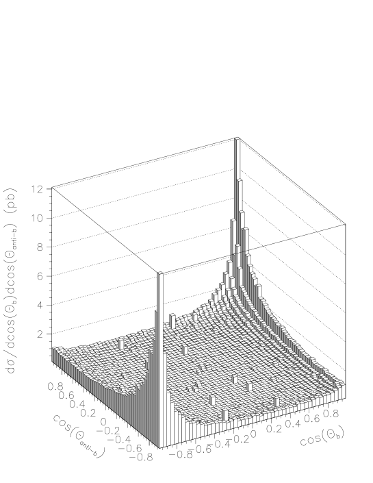
Figure 6.13: Distribution of the cosines of the polar angles of the botom and anti-bottom with respect to the beam line. The plot corresponds to single top production at the LHC with top decay included. The calculation was performed at the tree level in Standard Model with $\mu^{2}=\hat{s}=\left(q_{1}+q_{2}\right)^{2}$.

5 Conclusions

In this chapter we have performed a full analysis of the sensitivity of single top production in the s-channel to the presence of anomalous couplings in the effective electroweak theory. The analysis has been done in the context of the LHC experiments.

Unlike in the discussion concerning the single top production through the dominant t-channel, top decay has been considered. The only approximation involved is to consider the top as a real particle (narrow width approximation).

We have paid careful attention to the issue of the top polarization. We have argued, first of all, why it is not unjustified to neglect the interference term and to proceed as if the top spin was determined at an intermediate stage. We have provided a spin basis where the interference term is minimized. A similar analysis applies to the t-channel process. We present here and explicit basis for this case too. We get a sensitivity to $g_{R}$ in the same ballpark as the one obtained in the t-channel (where decay was not considered). Finally we have obtained that observables most sensible to $g_{R}$ are those where anti-lepton and bottom momenta are cut to be almost collinear.

Chapter 7 Results and Conclusions

Here we present a summary of the main results obtained in this thesis.

• In Chapter 2:

  • We present a complete classification of four-fermion operators giving mass to physical fermions and gauge vector bosons in models of dynamical symmetry breaking. This is done when new particles appear in the usual representations of the $SU(2)_{L}\times SU(3)_{c}$ group, and a partial classification it is done in the general case also. Only a single family is considered and therefore the problem of mixing is not addressed here.

  • We investigate the phenomenological consequences for the electroweak neutral sector of such class of models. This is done matching the four-fermion description to a lower energy theory that only contain all degrees of freedom of the SM (but the Higgs). The coefficients of such low energy effective Lagrangian for dynamical symmetry breaking models are then compared to those of models with elementary scalars (such as the minimal Standard Model).

  • We determine the value of the $Zb\bar{b}$ effective coupling in models of dynamical symmetry breaking and verify that the contribution is large, but its sign is not defined, contrary to some claims. The current value of this coupling is off the SM value by nearly a 3 $\sigma$ effect. We estimate the effects for light fermions too, where they are not observable at present. Some general observations concerning the mechanism of dynamical symmetry breaking are presented.

• In Chapter 3:

  • We analyze the structure of the four-dimensional effective operators in the electroweak matter sector when $CP$ violations and family mixing is allowed.

  • We perform the diagonalization of the mass and kinetic terms showing that, besides the presence of the CKM matrix in the SM charged vertex, new structures show up in the effective operators constructed with left handed fermions. In particular the CKM matrix is also present in the neutral sector.

  • We calculate also the contribution to the effective operators in the minimal SM with a heavy Higgs and in the SM supplemented with an additional heavy fermion doublet.

  • In general, even if the physics responsible for the generation of the additional effective operators is $CP$-conserving, phases which are present in the Yukawa and kinetic couplings become observable in the effective operators after diagonalization.

• In Chapter 4:

  • We present and solve the issue of defining a 1-loop set of wfr. constants consistent with the on-shell requirements and the gauge invariance of physical amplitudes. We demonstrate using Nielsen identities that our set of wfr. constants together with a gauge independent CKM renormalization yields gauge independent physical amplitudes for top and W decays.

  • We show that the previous on-shell prescription given in [19] does not diagonalize the propagator in family space and yields gauge dependent amplitudes for the charged electroweak vertex, albeit gauge independent modulus. This is not satisfactory since interference with e.g. strong phases may reveal an unacceptable gauge dependence. In the case of top decay we find that the numerical difference in the squared amplitude between our result and the one using the prescription in [19] amounts to a half per cent. This difference will be relevant to future experiments testing the $tb$ vertex.

  • We check the consistency of our scheme with the $CPT$ theorem. This is done showing that although our wfr. constants do not verify the pseudo-hermiticity condition ($\bar{Z}\neq\gamma^{0}Z^{\dagger}\gamma^{0}$) the total width of particles and anti-particles coincide.

• In Chapter 5:

  • We present a complete calculation of the t-channel cross sections for polarized tops or anti-tops including right effective couplings and bottom mass contributions.

  • We perform a Monte Carlo simulation of the production of single polarized tops at LHC presenting a variety of $p_{T}$ and angular distributions both for the $t$ and the $\bar{b}$ quarks. We show, without considering backgrounds or top decay, that we can expect a 2 $\sigma$ sensitivity to $g_{R}$ variations of the order of $5\times 10^{-2}.$

  • We show based on general theoretical grounds that the top cannot be produced in a pure spin state. Moreover we indicate which is the adequate spin basis to correctly fold top production cross section with top decay. This is necessary in order to calculate the whole process in the framework of the narrow width approximation.

• In Chapter 6:

  • We present a complete calculation of the s-channel cross section for single top production including top decay. Calculations include right effective couplings and bottom mass contributions.

  • We perform a Monte Carlo simulation of the production and decay of single polarized tops at LHC in the s-channel. We plot several $p_{T}$, invariant mass and angular distributions constructed with observable anti-lepton momentum and bottom and anti-bottom jets momenta. We find that variations of $g_{R}$ of the order of $5\times 10^{-2}$ are visible with signals ranging from $3$ to $1$ standard deviations depending on the phase of $g_{R}$ and the observables selected.

  • We present explicit expressions both for the t- and s- channels of the top spin basis that diagonalizes the top density matrix. We check numerically for the s-channel that such basis minimizes the interference terms not taken into account in the narrow width approximation.

Appendix A Conventions and useful formulae.

We use the metric $\eta_{\mu\nu}=\left(1,-1,-1,-1\right)$ and the Dirac representation with

$$\gamma^{0} = \left(\begin{array}[]{cc}I&0\\ 0&-I\end{array}\right),\quad\gamma^{i}=\left(\begin{array}[]{cc}0&\tau^{i}\\ -\tau^{i}&0\end{array}\right),\quad\gamma^{5}=i\gamma^{0}\gamma^{1}\gamma^{2}\gamma^{3}=\left(\begin{array}[]{cc}0&I\\ I&0\end{array}\right),$$

$$\tau^{1} = \left(\begin{array}[]{ll}0&1\\ 1&0\end{array}\right),\quad\tau^{2}=\left(\begin{array}[]{ll}0&-i\\ i&0\end{array}\right),\quad\tau^{3}=\left(\begin{array}[]{ll}1&0\\ 0&-1\end{array}\right),$$

$$\tau^{+} = \frac{\tau^{1}-i\tau^{2}}{\sqrt{2}}=\left(\begin{array}[]{ll}0&0\\ \sqrt{2}&0\end{array}\right),\quad\tau^{-}=\frac{\tau^{1}+i\tau^{2}}{\sqrt{2}}=\left(\begin{array}[]{ll}0&\sqrt{2}\\ 0&0\end{array}\right).$$

we also define the projectors

$$P_{\pm}=\frac{1\pm\gamma^{5}}{2},\tau^{u}=\frac{I+\tau^{3}}{2},\tau^{d}=\frac{I-\tau^{3}}{2},$$

where $P_{+}$ is the right projector ($R$), $P_{-}$ the left projector ($L$), $\tau^{u}$ is the up projector and $\tau^{d}$ the down projector satisfying

$$\left(P_{\pm}\right)^{2} = P_{\pm},$$

$$P_{+}P_{-} = P_{-}P_{+}=0,$$

$$P_{+}+P_{-} = I,$$

$$\left(\tau^{u}\right)^{2} = \tau^{u},$$

$$\left(\tau^{d}\right)^{2} = \tau^{d},$$

$$\tau^{u}\tau^{d} = \tau^{d}\tau^{u}=0,$$

$$\tau^{u}+\tau^{d} = I.$$

Let us write the matrices

$$G_{L}=e^{i\mathbf{\theta\cdot}\frac{\mathbf{\tau}}{2}},\qquad G_{R}=e^{i\beta\frac{\tau^{3}}{2}},\qquad G_{z}=e^{i\beta z},$$

where $\alpha,$ $\mathbf{\theta}$ and $\beta$ parametrize a representation of $SU\left(3\right)_{c}\times SU\left(2\right)_{L}\times U\left(1\right)_{Y}$, with $\mathbf{\tau}$ the Pauli matrices, $\mathbf{\lambda}$ the Gell-Mann matrices and $z$ a real parameter which takes the value $\frac{1}{6}$ for quarks and $\frac{-1}{2}$ for leptons. Then under $SU\left(3\right)_{c}\times SU\left(2\right)_{L}\times U\left(1\right)_{Y}$ we have that SM matter and gauge fields transform as

$$q_{L} \rightarrow G_{c}G_{\frac{1}{6}}G_{L}q_{L},$$

$$l_{L} \rightarrow G_{c}G_{\frac{-1}{2}}G_{L}l_{L},$$

$$q_{R} \rightarrow G_{c}G_{\frac{1}{6}}G_{R}q_{R},$$

$$l_{R} \rightarrow G_{c}G_{\frac{-1}{2}}G_{R}l_{R},$$

$$U \rightarrow G_{L}UG_{R}^{\dagger},$$

$$\frac{\mathbf{\tau}}{2}\mathbf{\cdot W}_{\mu} \rightarrow G_{L}\left(\frac{\mathbf{\tau}}{2}\mathbf{\cdot W}_{\mu}-\frac{i}{g}\partial_{\mu}\right)G_{L}^{\dagger}$$

$$\frac{\tau^{3}}{2}B_{\mu} \rightarrow \frac{\tau^{3}}{2}B_{\mu}-\frac{i}{g^{\prime}}G_{R}\partial_{\mu}G_{R}^{\dagger},$$

$$\frac{\mathbf{\lambda}}{2}\mathbf{\cdot G}_{\mu} \rightarrow G_{c}\left(\frac{\mathbf{\lambda}}{2}\mathbf{\cdot G}_{\mu}-\frac{i}{g_{s}}\partial_{\mu}\right)G_{c}^{\dagger}.$$ (A.4)

These transformations allow for the covariant derivatives

$$D_{\mu}U = \partial_{\mu}U+ig\frac{\mathbf{\tau}}{2}\mathbf{\cdot W}_{\mu}U-ig^{\prime}U\frac{\tau^{3}}{2}B_{\mu},$$

$$D_{\mu}^{L}f_{L} = \partial_{\mu}f_{L}+ig\frac{\mathbf{\tau}}{2}\mathbf{\cdot W}_{\mu}f_{L}+ig^{\prime}\left(\frac{\tau^{3}}{2}-Q\right)B_{\mu}f_{L}+ig_{s}\frac{\mathbf{\lambda}}{2}\mathbf{\cdot G}_{\mu}f_{L},$$

$$D_{\mu}^{R}f_{R} = \partial_{\mu}f_{R}+ig^{\prime}QB_{\mu}f_{R}+ig_{s}\frac{\mathbf{\lambda}}{2}\mathbf{\cdot G}_{\mu}f_{R},$$

where the charge $Q$ and hypercharge $Y$ are given by

$$Q=\frac{\tau^{3}}{2}+z,\qquad Y=\left\{\begin{tabular}[]{ll}$z$&$\mathrm{for\ lefts}$\\ $\frac{\tau^{3}}{2}+z$&$\mathrm{for\ rights}$\end{tabular}\right.,$$

It is useful also to introduce the notation

$$\tau^{\pm}\equiv\frac{\tau^{1}\mp i\tau^{2}}{\sqrt{2}},\qquad W_{\mu}^{\pm}\equiv\frac{W_{\mu}^{1}\mp iW_{\mu}^{2}}{\sqrt{2}}.$$

when diagonalizing the mass matrices we perform

$$W_{\mu}^{3} = s_{W}A_{\mu}+c_{W}Z_{\mu},$$

$$B_{\mu} = c_{W}A_{\mu}-s_{W}Z_{\mu},$$

$$s_{W} \equiv \sin\theta_{W}\equiv\frac{g^{\prime}}{\sqrt{g^{2}+g^{\prime\,2}}},$$

$$c_{W} \equiv \cos\theta_{W}\equiv\frac{g}{\sqrt{g^{2}+g^{\prime\,2}}},$$

$$e \equiv gs_{W}=g^{\prime}c_{W},$$

obtaining the SM kinetic term given by Eq.(3.18)

1 Some facts

We have

$$\left\{\gamma^{\mu},\gamma^{\nu}\right\} = 2\eta^{\mu\nu},$$

$$\gamma^{0}\gamma^{\mu}\gamma^{0} = \gamma^{\mu\dagger}=\gamma_{\mu},$$

$$\gamma^{2}\gamma^{\mu}\gamma^{2} = \gamma^{\mu\ast},$$

we also have

$$\left(D_{\mu}U\right)^{\dagger}U = \left(\partial_{\mu}U^{\dagger}-igU^{\dagger}\frac{\mathbf{\tau}}{2}\mathbf{\cdot W}_{\mu}+ig^{\prime}\frac{\tau^{3}}{2}U^{\dagger}B_{\mu}\right)$$

$$= -U^{\dagger}\partial_{\mu}U-igU^{\dagger}\frac{\mathbf{\tau}}{2}\mathbf{\cdot W}_{\mu}U+ig^{\prime}U^{\dagger}U\frac{\tau^{3}}{2}B_{\mu}$$

$$= -U^{\dagger}D_{\mu}U,$$

and

$$U^{\intercal}\tau^{2} = \tau^{2}U^{\dagger},$$

$$\left(D_{\mu}U\right)^{\intercal}\tau^{2} = \tau^{2}\left(D_{\mu}U\right)^{\dagger}.$$

and for a $2\times 2$ matrix $A$ we have

$$\det\left(A\right)=\frac{\epsilon^{lm}\epsilon^{ij}}{2}A_{il}A_{jm}=-\frac{1}{2}Tr\left(\epsilon A\epsilon A^{\intercal}\right)=\frac{1}{2}Tr\left(\tau^{2}A\tau^{2}A^{\intercal}\right),$$

Other useful properties are

$$\left[\tau^{i},\tau^{j}\right] = i2\epsilon^{ijk}\tau^{k},$$

$$\left\{\tau^{i},\tau^{j}\right\} = 2\delta^{ij},$$

implying

$$e^{-i\eta_{i}\frac{\tau^{i}}{2}}\tau^{p}e^{i\eta_{j}\frac{\tau^{j}}{2}} = \tau^{p}+\left[\tau^{p},i\eta_{j}\frac{\tau^{j}}{2}\right]+\frac{1}{2!}\left[\left[\tau^{p},i\eta_{j}\frac{\tau^{j}}{2}\right],i\eta_{k}\frac{\tau^{k}}{2}\right]+\cdots$$

$$= \tau^{p}-\eta_{j}\epsilon^{pjk}\tau^{k}+\frac{\left(-1\right)^{2}}{2!}\eta_{j}\eta_{k}\epsilon^{pjl}\epsilon^{lkm}\tau^{m}+\cdots$$

$$= \left(e^{A}\right)_{pk}\tau^{k},$$

where

$$A_{ij}\equiv\epsilon^{ijk}\eta_{k}.$$

and finally it will be useful to keep the following set of algebraic relations

$$\left\{\tau^{3},\tau^{\pm}\right\} = 0,$$

$$\tau^{3}\tau^{\pm} = \mp\tau^{\pm},$$

$$\tau^{\pm}\tau^{3} = \pm\tau^{\pm},$$

$$\tau^{+}\tau^{d} = \tau^{d}\tau^{-}=\tau^{-}\tau^{u}=\tau^{u}\tau^{+}=0,$$

$$\tau^{-}\tau^{d} = \tau^{u}\tau^{-}=\tau^{-},$$

$$\tau^{+}\tau^{u} = \tau^{d}\tau^{+}=\tau^{+},$$

$$\left(\tau^{+}\right)^{2} = \left(\tau^{-}\right)^{2}=0,$$

$$\left(\tau^{u}\right)^{2} = \tau^{u},$$

$$\left(\tau^{d}\right)^{2} = \tau^{d},$$

$$\tau^{u}\tau^{d} = \tau^{d}\tau^{u}=0,$$

$$\tau^{+}\tau^{-} = 2\tau^{u},$$

$$\tau^{-}\tau^{+} = 2\tau^{d}.$$

The Dirac spinors used for calculations are given by

$$u^{\left(+\right)}\left(p\right) = \frac{\not{p}+m}{\sqrt{2m\left(m+p^{0}\right)}}\left(\begin{array}[]{c}1\\ 0\\ 0\\ 0\end{array}\right),\qquad u^{\left(-\right)}\left(p\right)=\frac{\not{p}+m}{\sqrt{2m\left(m+p^{0}\right)}}\left(\begin{array}[]{c}0\\ 1\\ 0\\ 0\end{array}\right),$$

$$v^{\left(+\right)}\left(p\right) = \frac{-\not{p}+m}{\sqrt{2m\left(m+p^{0}\right)}}\left(\begin{array}[]{c}0\\ 0\\ 0\\ 1\end{array}\right),\qquad v^{\left(-\right)}\left(p\right)=\frac{-\not{p}+m}{\sqrt{2m\left(m+p^{0}\right)}}\left(\begin{array}[]{c}0\\ 0\\ 1\\ 0\end{array}\right),$$

$$\bar{u}^{\left(s\right)}\left(p\right) = u^{\left(s\right)\dagger}\left(p\right)\gamma^{0},$$

$$\bar{v}^{\left(s\right)}\left(p\right) = v^{\left(s\right)\dagger}\left(p\right)\gamma^{0},$$

hence

$$\left(i\gamma^{0}\gamma^{2}\right)\bar{u}^{\left(s\right)T}\left(p\right) = -i\gamma^{2}u^{\left(s\right)\ast}\left(p\right)$$

$$= -i\gamma^{2}\frac{\not{p}^{\ast}+m}{\sqrt{2m\left(m+p^{0}\right)}}u^{\left(s\right)}\left(\left(m,0\right)\right)$$

$$= \frac{-\not{p}+m}{\sqrt{2m\left(m+p^{0}\right)}}\left(-i\gamma^{2}\right)u^{\left(s\right)}\left(\left(m,0\right)\right)$$

$$= \frac{-\not{p}+m}{\sqrt{2m\left(m+p^{0}\right)}}\left(\begin{array}[]{cccc}0&0&0&-1\\ 0&0&1&0\\ 0&1&0&0\\ -1&0&0&0\end{array}\right)u^{\left(s\right)}\left(\left(m,0\right)\right)$$

$$= -sv^{\left(s\right)}\left(p\right),$$

and

$$i\gamma^{2}\bar{u}^{\left(s\right)T}\left(p\right) = -i\gamma^{0}\gamma^{2}u^{\left(s\right)\ast}\left(p\right)$$

$$= -i\gamma^{0}\gamma^{2}\frac{\not{p}^{\ast}+m}{\sqrt{2m\left(m+p^{0}\right)}}u^{\left(s\right)}\left(\left(m,0\right)\right)$$

$$= \frac{-\tilde{\not{p}}+m}{\sqrt{2m\left(m+p^{0}\right)}}\left(-i\gamma^{0}\gamma^{2}\right)u^{\left(s\right)}\left(\left(m,0\right)\right)$$

$$= \frac{-\tilde{\not{p}}+m}{\sqrt{2m\left(m+p^{0}\right)}}\left(\begin{array}[]{cccc}0&0&0&-1\\ 0&0&1&0\\ 0&-1&0&0\\ 1&0&0&0\end{array}\right)u^{\left(s\right)}\left(\left(m,0\right)\right)$$

$$= sv^{\left(s\right)}\left(\tilde{p}\right),$$

with

$$\tilde{p}^{\mu}=p_{\mu}=\left(p^{0},-\vec{p}\right),$$

and

$$u^{\left(s\right)T}\left(p\right)i\gamma^{2} = u^{\left(s\right)T}\left(\left(m,0\right)\right)\frac{\not{p}^{T}+m}{\sqrt{2m\left(m+p^{0}\right)}}i\gamma^{2}$$

$$= u^{\left(s\right)T}\left(\left(m,0\right)\right)i\gamma^{2}\frac{-\tilde{\not{p}}+m}{\sqrt{2m\left(m+p^{0}\right)}}$$

$$= u^{\left(s\right)T}\left(\left(m,0\right)\right)\left(\begin{array}[]{cccc}0&0&0&1\\ 0&0&-1&0\\ 0&-1&0&0\\ 1&0&0&0\end{array}\right)\frac{-\tilde{\not{p}}+m}{\sqrt{2m\left(m+p^{0}\right)}}$$

$$= sv^{\left(s\right)T}\left(\left(m,0\right)\right)\frac{-\tilde{\not{p}}+m}{\sqrt{2m\left(m+p^{0}\right)}}\gamma^{0}\gamma^{0}$$

$$= -sv^{\left(s\right)T}\left(\left(m,0\right)\right)\frac{-\tilde{\not{p}}^{\dagger}+m}{\sqrt{2m\left(m+p^{0}\right)}}\gamma^{0}$$

$$= -s\bar{v}^{\left(s\right)}\left(\tilde{p}\right),$$

and summing up we have

$$i\gamma^{2}\bar{u}^{\left(s\right)T}\left(p\right) = sv^{\left(s\right)}\left(\tilde{p}\right),$$

$$u^{\left(s\right)T}\left(p\right)i\gamma^{2} = -s\bar{v}^{\left(s\right)}\left(\tilde{p}\right).$$ (A.10)

Appendix B Matter sector appendices

1 $d=4$ operators

The procedure we have followed to obtain operators (2.8–2.15) is very simple. We have to look for operators of the form $\bar{\psi}\Gamma\psi$, where $\psi=q_{L},\;q_{R}$ and $\Gamma$ contains a covariant derivative, $D_{\mu}$, and an arbitrary number of $U$ matrices. These operators must be gauge invariant so not any form of $\Gamma$ is possible. Moreover, we can drop total derivatives and, since $U$ is unitary, we have the following relation

$$D_{\mu}U=-U(D_{\mu}U)^{\dagger}U.$$ (B.1)

Apart from the obvious structure $D_{\mu}U$ which transform as $U$ does, we immediately realize that the particular form of $G_{R}$ implies the following simple transformations for the combinations $U\tau^{3}U^{\dagger}$ and $(D_{\mu}U)\tau^{3}U^{\dagger}$

$$U\tau^{3}U^{\dagger} \mapsto G_{L}\;U\tau^{3}U^{\dagger}\;G_{L}^{\dagger}$$ (B.2)

$$(D_{\mu}U)\tau^{3}U^{\dagger} \mapsto G_{L}\;(D_{\mu}U)\tau^{3}U^{\dagger}\;G_{L}^{\dagger}$$ (B.3)

Keeping all these relations in mind, we simply write down all the possibilities for $\bar{\psi}\Gamma\psi$ and find the list of operators (2.8–2.15). It is worth mentioning that there appears to be another family of four operators in which the $U$ matrices also occur within a trace: $\bar{\psi}\Gamma\psi\;Tr\Gamma^{\prime}$. One can check, however, that these are not independent. More precisely, using the remarkable identities

$$i\left(D_{\mu}U\right)\tau^{3}U^{\dagger}+h.c. = i\tau^{3}U^{\dagger}\left(D_{\mu}U\right)+h.c$$

$$= iTr\left(\left(D_{\mu}U\right)\tau^{3}U^{\dagger}\right),$$

we have

$$i\bar{q}_{L}\gamma^{\mu}q_{L}\;Tr\left[(D_{\mu}U)\tau^{3}U^{\dagger}\right] = \frac{1}{M_{L}^{2}}\mathcal{L}_{L}^{2},$$ (B.4)

$$i\bar{q}_{L}\gamma^{\mu}U\tau^{3}U^{\dagger}q_{L}\;Tr\left[(D_{\mu}U)\tau^{3}U^{\dagger}\right] = \frac{1}{2M_{L}^{3}}\mathcal{L}_{L}^{3}-\frac{1}{2M_{L}^{1}}\mathcal{L}_{L}^{1},$$ (B.5)

$$i\bar{q}_{R}\gamma^{\mu}q_{R}\;Tr\left[(D_{\mu}U)\tau^{3}U^{\dagger}\right] = \frac{1}{M_{R}^{2}}\mathcal{L}_{R}^{2},$$ (B.6)

$$i\bar{q}_{R}\gamma^{\mu}\tau^{3}q_{R}\;Tr\left[(D_{\mu}U)\tau^{3}U^{\dagger}\right] = \frac{1}{2M_{R}^{1}}\mathcal{L}_{R}^{1}+\frac{1}{2M_{R}^{3}}\mathcal{L}_{R}^{3},$$ (B.7)

Note that $\mathcal{L}_{L}^{4}$ (as well as $\mathcal{L}_{R}^{\prime}$ discussed above) can be reduced by equations of motion to operators of lower dimension which do not contribute to the physical processes we are interested in. We have checked that its contribution indeed drops from the relevant $S$-matrix elements.

2 Feynman rules

We write the effective $d=4$ Lagrangian as

$$\mathcal{L}_{c}{}_{\mathrm{eff}}=\sum_{k=1}^{3}\left(\mathcal{L}_{L}^{k}+\mathcal{L}_{R}^{k}\right)+\mathcal{L}_{L}^{4}+\mathcal{L}_{R}^{\prime},$$

where the real coefficients $M_{L,R}^{i}$ appearing in the definitions (2.8-2.15) are to be determined through the matching. We need to match the effective theory described by $\mathcal{L}_{c}{}_{\mathrm{eff}}$ to both, the MSM and the underlying theory parametrized by the four-fermion operators. It has proven more convenient to work with the physical fields $W^{\pm}$, $Z$ and $\gamma$ in the former case whereas the use of the Lagrangian fields $W^{1}$, $W^{2}$, $W^{3}$ and $B$ is clearly more straightforward for the latter. Thus, we give the Feynman rules in terms of both the physical and unphysical basis.

(B.8)

$$-\left.\left(1-{\frac{2}{3}}s_{W}^{2}\right)M_{L}^{4}+{\frac{1}{3}}s_{W}^{2}\;M_{R}^{\prime}\right\}$$

$$+ {\frac{ie}{2s_{W}c_{W}}}\gamma_{\mu}\gamma_{5}\left\{\frac{1}{2}\left(2M_{L}^{1}+2M_{R}^{1}-2M_{L}^{3}+2M_{R}^{3}\right)+M_{L}^{2}-M_{R}^{2}\right.$$

$$\left.+\left(1-{\frac{2}{3}}s_{W}^{2}\right)M_{L}^{4}+{\frac{1}{3}}s_{W}^{2}\;M_{R}^{\prime}\right\},$$

(B.9)

$$-\left.\left(1-{\frac{4}{3}}s_{W}^{2}\right)M_{L}^{4}+{\frac{2}{3}}s_{W}^{2}\;M_{R}^{\prime}\right\}$$

$$+ {\frac{ie}{2s_{W}c_{W}}}\gamma_{\mu}\gamma_{5}\left\{\frac{1}{2}\left(-2M_{L}^{1}-2M_{R}^{1}+2M_{L}^{3}-2M_{R}^{3}\right)+M_{L}^{2}-M_{R}^{2}\right.$$

$$+\left.\left(1-{\frac{4}{3}}s_{W}^{2}\right)M_{L}^{4}+{\frac{2}{3}}s_{W}^{2}\;M_{R}^{\prime}\right\},$$

(B.10)

(B.11)

(B.12)

$$+ ie{\frac{1}{2\sqrt{2}s_{W}}}\gamma_{\mu}\gamma_{5}\left(2M_{L}^{1}+2M_{L}^{3}+2M_{R}^{1}+2M_{R}^{3}\right).$$

The operators $\mathcal{L}_{L}^{4}$ and $\mathcal{L}_{R}^{\prime}$ contribute to two-point function. The relevant Feynman rules are

(B.13)

(B.14)

Rather than giving the actual Feynman rules in the unphysical basis, we collect the various tensor structures that can result from the calculation of the relevant diagrams in table 2.1.

$$\begin{array}[]{l||c|c|c|c|c|c|}Tensor~{}structure&M_{L}^{1}&M_{L}^{2}&M_{L}^{3}&M_{R}^{1}&M_{R}^{2}&M_{R}^{3}\\ \hline\cr i\bar{q}_{L}\,g[\tau^{1}\not{W}^{1}+\tau^{2}\not{W}^{2}]q_{L}&1&&1&&&\\ i\bar{q}_{L}\,\tau^{3}[g\not{W}^{3}-g^{\prime}\not{B}]q_{L}&1&&-1&&&\\ i\bar{q}_{L}\,[g\not{W}^{3}-g^{\prime}\not{B}]q_{L}&&-1&&&&\\ i\bar{q}_{R}\,g[\tau^{1}\not{W}^{1}+\tau^{2}\not{W}^{2}]q_{R}&&&&-1&&1\\ i\bar{q}_{R}\,\tau^{3}[g\not{W}^{3}-g^{\prime}\not{B}]q_{R}&&&&-1&&-1\\ i\bar{q}_{R}\,[g\not{W}^{3}-g^{\prime}\not{B}]q_{R}&&&&&-1&\end{array}$$

Table 2.1: Various structures appearing in the matching of the vertex and the corresponding contributions to $\mathcal{L}_{L,R}^{1,2,3}$

We include only those that can be matched to insertions of the operators $\mathcal{L}_{L,R}^{1,2,3}$ (the contributions to $\mathcal{L}_{L}^{4}$ and $\mathcal{L}_{R}^{\prime}$ can be determined from the matching of the two-point functions). The corresponding contributions of these structures to $M_{L,R}^{1},$ $M_{L,R}^{2}$ and $M_{L,R}^{3}$ are also given in table 2.1. Once $M_{L}^{4}$ has been replaced by its value, obtained in the matching of the two-point functions, only the listed structures can show up in the matching of the vertex, otherwise the $SU(2)\times U(1)$ symmetry would not be preserved.

3 Four-fermion operators

The complete list of four-fermion operators relevant for the discussion in section 5 of Chapter 2 is in tables 2.1 and 2.2 of that section. It is also explained in that section the convenience of fierzing the operators in the last seven rows of table 2.1 in order to write them in the form $\mathbf{J}\cdot\mathbf{j}$. Here we just give the list that comes out naturally from our analysis, tables 2.1 and 2.2, without further physical interpretation. The list is given for fermions belonging to the representation $\mathbf{3}$ of $SU(3)_{c}$ (techniquarks). By using Fierz transformations one can easily find out relations among some of these operators when the fermions are color singlet (technileptons), which is telling us that some of these operators are not independent in this case. A list of independent operators for technileptons is also given in section 5 of Chapter 2. In particular, the independent chirality preserving operators for colorless fermions are in the first six rows of table 2.1 (those whose name we write in capital letters) and, additionally, only the two operators $\left(\bar{Q}_{L}\gamma_{\mu}q_{L}\right)\left(\bar{q}_{L}\gamma^{\mu}Q_{L}\right),$ $\left(\bar{Q}_{R}\gamma_{\mu}q_{R}\right)\left(\bar{q}_{R}\gamma^{\mu}Q_{R}\right)$ from the last seven rows.

Let us outline the procedure we have followed to obtain this basis in the (more involved) case of colored fermions.

There are only two color singlet structures one can build out of four fermions, namely ($\alpha,$ $\beta,$ … are color indices)

$$(\bar{\psi}\psi)(\bar{\psi}^{\prime}\psi^{\prime}) \equiv \bar{\psi}_{\alpha}\psi_{\alpha}\;\bar{\psi}_{\beta}^{\prime}\psi_{\beta}^{\prime}\;,$$ (B.15)

$$(\bar{\psi}\vec{\lambda}\psi)\cdot(\bar{\psi}^{\prime}\vec{\lambda}\psi^{\prime}) \equiv \bar{\psi}_{\alpha}(\vec{\lambda})_{\alpha\beta}\psi_{\beta}\;\cdot\;\bar{\psi}_{\gamma}^{\prime}(\vec{\lambda})_{\gamma\delta}\psi_{\delta}^{\prime}\;,$$ (B.16)

where, $\psi$ stands for any field belonging to the representation $\mathbf{3}$ of $SU(3)_{c}$ ($\psi$ will be either $q$ or $Q$); $\alpha$, $\beta$,…, are color indices; and the primes ( ^′) remind us that $\psi$ and $\bar{\psi}$ carry the same additional indices (Dirac, $SU(2)$, …).

Next we classify the Dirac structures. Since $\psi$ is either $\psi_{L}$ [it belongs to the representation $(\frac{1}{2},0)$ of the Lorentz group] or $\psi_{R}$ [representation $(0,\frac{1}{2})$], we have five sets of fields to analyze, namely

$$\{\bar{\psi}_{L},\psi_{L},\bar{\psi}_{L}^{\prime},\psi_{L}^{\prime}\},\quad[R\leftrightarrow L];\qquad\{\bar{\psi}_{L},\psi_{L},\bar{\psi}_{R},\psi_{R}\};$$ (B.17)

$$\{\bar{\psi}_{L},\psi_{R},\bar{\psi}_{L}^{\prime},\psi_{R}^{\prime}\},\qquad[R\leftrightarrow L].$$ (B.18)

There is only an independent scalar we can build with each of the three sets in (B.17). Our choice is

$$\bar{\psi}_{L}\gamma^{\mu}\psi_{L}\;\bar{\psi}_{L}^{\prime}\gamma_{\mu}\psi_{L}^{\prime},\qquad[R\leftrightarrow L];$$ (B.19)

$$\bar{\psi}_{L}\gamma^{\mu}\psi_{L}\;\bar{\psi}_{R}\gamma_{\mu}\psi_{R}.$$ (B.20)

where the prime is not necessary in the second equation because $R$ and $L$ suffice to remind us that the two $\psi$ and $\bar{\psi}$ may carry different ($SU(2)$, technicolor, …) indices. There appear to be four other independent scalar operators: $\bar{\psi}_{L}\gamma^{\mu}\psi_{L}^{\prime}\;\bar{\psi}_{L}^{\prime}\gamma_{\mu}\psi_{L}$, $[R\leftrightarrow L]$; $\allowbreak\bar{\psi}_{L}\psi_{R}\;\bar{\psi}_{R}\psi_{L}$; and $\bar{\psi}_{L}\sigma^{\mu\nu}\psi_{R}\;\bar{\psi}_{R}\sigma_{\mu\nu}\psi_{L}$. However, Fierz symmetry implies that the first three are not independent, and the fourth one vanishes, as can be also seen using the identity $2i\sigma^{\mu\nu}\gamma^{5}=\epsilon^{\mu\nu\rho\lambda}\sigma_{\rho\lambda}$. For each of the two operators in (B.18), two independent scalars can be constructed. Our choice is

$$\bar{\psi}_{L}\psi_{R}\;\bar{\psi}_{L}^{\prime}\psi_{R}^{\prime},\qquad[R\leftrightarrow L];$$ (B.21)

$$\bar{\psi}_{L}\psi_{R}^{\prime}\;\bar{\psi}_{L}^{\prime}\psi_{R},\qquad[R\leftrightarrow L].$$ (B.22)

Again, there appear to be four other scalar operators: $\bar{\psi}_{L}\sigma^{\mu\nu}\psi_{R}\;\bar{\psi}_{L}^{\prime}\sigma_{\mu\nu}\psi_{R}^{\prime}$, $[R\leftrightarrow L]$;$\bar{\psi}_{L}\sigma^{\mu\nu}\psi_{R}^{\prime}\;\bar{\psi}_{L}^{\prime}\sigma_{\mu\nu}\psi_{R}$, $[R\leftrightarrow L]$; which, nevertheless, can be shown not to be independent but related to (B.21) and (B.22) by Fierz symmetry. To summarize, the independent scalar structures are (B.19), (B.20), (B.21) and (B.22).

Next, we combine the color and the Dirac structures. We do this for the different cases (B.19) to (B.22) separately. For operators of the form (B.19), we have the two obvious possibilities (Hereafter, color and Dirac indices will be implicit)

$$(\bar{\psi}_{L}\gamma^{\mu}\psi_{L})(\bar{\psi}_{L}^{\prime}\gamma_{\mu}\psi_{L}^{\prime}),\qquad[R\leftrightarrow L];$$ (B.23)

$$(\bar{\psi}_{L}\gamma^{\mu}\psi_{L}^{\prime})(\bar{\psi}_{L}^{\prime}\gamma_{\mu}\psi_{L}),\qquad[R\leftrightarrow L];$$ (B.24)

where fields in parenthesis have their color indices contracted as in (B.15) and (B.16). Note that the operator $(\bar{\psi}_{L}\gamma^{\mu}\vec{\lambda}\psi_{L})\cdot(\bar{\psi}_{L}^{\prime}\gamma_{\mu}\vec{\lambda}\psi_{L}^{\prime})$, or its $R$ version, is not independent (recall that $(\vec{\lambda})_{\alpha\beta}\cdot(\vec{\lambda})_{\gamma\delta}=2\delta_{\alpha\delta}\delta_{\beta\gamma}-2/3\;\delta_{\alpha\beta}\delta_{\gamma\delta}$). For operators of the form (B.20), we take

$$(\bar{\psi}_{L}\gamma^{\mu}\psi_{L})(\bar{\psi}_{R}\gamma_{\mu}\psi_{R}),$$ (B.25)

$$(\bar{\psi}_{L}\gamma^{\mu}\vec{\lambda}\psi_{L})\cdot(\bar{\psi}_{R}\gamma_{\mu}\vec{\lambda}\psi_{R}),$$ (B.26)

Finally, for operators of the form (B.21) and (B.22), our choice is

$$(\bar{\psi}_{L}\psi_{R})(\bar{\psi}_{L}^{\prime}\psi_{R}^{\prime}),\quad[R\leftrightarrow L];\quad(\bar{\psi}_{L}\vec{\lambda}\psi_{R})\cdot(\bar{\psi}_{L}^{\prime}\vec{\lambda}\psi_{R}^{\prime}),\quad[R\leftrightarrow L];$$ (B.27)

$$(\bar{\psi}_{L}\psi_{R}^{\prime})(\bar{\psi}_{L}^{\prime}\psi_{R}),\quad[R\leftrightarrow L];\quad(\bar{\psi}_{L}\vec{\lambda}\psi_{R}^{\prime})\cdot(\bar{\psi}_{L}^{\prime}\vec{\lambda}\psi_{R}),\quad[R\leftrightarrow L].$$ (B.28)

All them are independent unless further symmetries [e.g., $SU(2)_{L}\times SU(2)_{R}$] are introduced.

To introduce the $SU(2)_{L}\times SU(2)_{R}$ symmetry one just assigns $SU(2)$ indices ($i$, $j$, $k$, …) to each of the fields in (B.23–B.28). We can drop the primes hereafter since there is no other symmetry left but technicolor which for the present analysis is trivial (recall that we are only interested in four fermion operators of the form $Q\bar{Q}q\bar{q}$, thus technicolor indices must necessarily be matched in the obvious way: $Q^{A}\bar{Q}^{A}q\bar{q}$). For each of the operators in (B.23) and (B.24), there are two independent ways of constructing $SU(2)_{L}\times SU(2)_{R}$ invariants. Only two of the four resulting operators turn out to be independent (actually, the other two are exactly equal to the first ones). The independent operators are chosen to be

$$(\bar{\psi}_{L}^{i}\gamma^{\mu}\psi_{L}^{i})(\bar{\psi}_{L}^{j}\gamma_{\mu}\psi_{L}^{j})\equiv(\bar{\psi}_{L}\gamma^{\mu}\psi_{L})(\bar{\psi}_{L}\gamma_{\mu}\psi_{L}),\quad[R\leftrightarrow L];$$ (B.29)

$$(\bar{\psi}_{L}^{i}\gamma^{\mu}\psi_{L}^{j})(\bar{\psi}_{L}^{j}\gamma_{\mu}\psi_{L}^{i}),\quad[R\leftrightarrow L];$$ (B.30)

For each of the operators in (B.25–B.28), the same straightforward group analysis shows that there is only one way to construct a $SU(2)_{L}\times SU(2)_{R}$ invariant. Discarding the redundant operators and imposing hermiticity and $CP$ invariance one finally has, in addition to the operators (B.29) and (B.30), those listed below (from now on, we understand that fields in parenthesis have their Dirac, color and also flavor indices contracted as in (B.29))

$$(\bar{\psi}_{L}\gamma^{\mu}\psi_{L})(\bar{\psi}_{R}\gamma_{\mu}\psi_{R}),$$ (B.31)

$$(\bar{\psi}_{L}\gamma^{\mu}\vec{\lambda}\psi_{L})\cdot(\bar{\psi}_{R}\gamma_{\mu}\vec{\lambda}\psi_{R}),$$ (B.32)

$$(\bar{\psi}_{L}^{i}\psi_{R}^{j})(\bar{\psi}_{L}^{k}\psi_{R}^{l})\epsilon_{ik}\epsilon_{jl}+(\bar{\psi}_{R}^{i}\psi_{L}^{j})(\bar{\psi}_{R}^{k}\psi_{L}^{l})\epsilon_{ik}\epsilon_{jl},$$ (B.33)

$$(\bar{\psi}_{L}^{i}\vec{\lambda}\psi_{R}^{j})\cdot(\bar{\psi}_{L}^{k}\vec{\lambda}\psi_{R}^{l})\epsilon_{ik}\epsilon_{jl}+(\bar{\psi}_{R}^{i}\vec{\lambda}\psi_{L}^{j})\cdot(\bar{\psi}_{R}^{k}\vec{\lambda}\psi_{L}^{l})\epsilon_{ik}\epsilon_{jl}.$$ (B.34)

We are now in a position to obtain very easily the custodially preserving operators of tables 2.1 and 2.2 We simply replace $\psi$ by $q$ and $Q$ (a pair of each: a field and its conjugate) in all possible independent ways.

To break the custodial symmetry we simply insert $\tau^{3}$ matrices in the $R$-sector of the custodially preserving operators we have just obtain (left columns of tables 2.1 and 2.2). However, not all the operators obtained this way are independent since one can prove the following relations

$$(\bar{q}_{R}^{i}\gamma^{\mu}Q_{R}^{j})(\bar{Q}_{R}^{j}\gamma_{\mu}[\tau^{3}q_{R}]^{i}) = (\bar{q}_{R}\gamma^{\mu}\tau^{3}Q_{R})(\bar{Q}_{R}\gamma_{\mu}q_{R})+(\bar{q}_{R}\gamma^{\mu}Q_{R})(\bar{Q}_{R}\gamma_{\mu}\tau^{3}q_{R})$$ (B.35)

$$\qquad-(\bar{q}_{R}^{i}\gamma^{\mu}[\tau^{3}Q_{R}]^{j})(\bar{Q}_{R}^{j}\gamma_{\mu}q_{R}^{i}),$$

$$(\bar{q}_{R}^{i}\gamma^{\mu}[\tau^{3}Q_{R}]^{j})(\bar{Q}_{R}^{j}\gamma_{\mu}[\tau^{3}q_{R}]^{i}) = (\bar{q}_{R}\gamma^{\mu}Q_{R})(\bar{Q}_{R}\gamma_{\mu}q_{R})+(\bar{q}_{R}\gamma^{\mu}\tau^{3}Q_{R})(\bar{Q}_{R}\gamma_{\mu}\tau^{3}q_{R})$$ (B.36)

$$\qquad-(\bar{q}_{R}^{i}\gamma^{\mu}Q_{R}^{j})(\bar{Q}_{R}^{j}\gamma_{\mu}q_{R}^{i}),$$

$$(\bar{q}_{R}^{i}\gamma^{\mu}[\tau^{3}q_{R}]^{j})(\bar{Q}_{R}^{j}\gamma_{\mu}[\tau^{3}Q_{R}]^{i}) = (\bar{q}_{R}\gamma^{\mu}q_{R})(\bar{Q}_{R}\gamma_{\mu}Q_{R})+(\bar{q}_{R}\gamma^{\mu}\tau^{3}q_{R})(\bar{Q}_{R}\gamma_{\mu}\tau^{3}Q_{R})$$

$$\qquad-(\bar{q}_{R}^{i}\gamma^{\mu}q_{R}^{j})(\bar{Q}_{R}^{j}\gamma_{\mu}Q_{R}^{i}),$$

$$(\bar{q}_{R}^{i}\gamma^{\mu}[\tau^{3}q_{R}]^{j})(\bar{Q}_{R}^{j}\gamma_{\mu}Q_{R}^{i})\qquad\phantom{+}$$

$$+(\bar{q}_{R}^{i}\gamma^{\mu}q_{R}^{j})(\bar{Q}_{R}^{j}\gamma_{\mu}[\tau^{3}Q_{R}]^{i}) = (\bar{q}_{R}\gamma^{\mu}q_{R})(\bar{Q}_{R}\gamma^{\mu}\tau^{3}Q_{R})$$ (B.38)

$$\qquad+(\bar{q}_{R}\gamma^{\mu}\tau^{3}q_{R})(\bar{Q}_{R}\gamma^{\mu}Q_{R}).$$

Our final choice of custodially breaking operators is the one in the right columns of tables 2.1 and 2.2.

4 Renormalization of the matter sector

Although most of the material in this section is standard, it is convenient to collect some of the important expressions, as the renormalization of the fermion fields is somewhat involved, and also to set up the notation. Let us introduce three wave-function renormalization constants for the fermion fields

$$\left(\begin{array}[]{c}u\\ d\end{array}\right)_{L} \rightarrow Z_{L}^{1/2}\left(\begin{array}[]{c}u\\ d\end{array}\right)_{L},$$ (B.43)

$$u_{R} \rightarrow (Z_{R}^{u})^{1/2}u_{R},$$ (B.44)

$$d_{R} \rightarrow (Z_{R}^{d})^{1/2}d_{R}.$$ (B.45)

where $u$ ($d$) stands for the field of the up-type (down-type) fermion. We write

$$Z_{i}=1+\delta Z_{i}$$ (B.46)

We also renormalize the fermion masses according to

$$m_{f}\rightarrow m_{f}+\delta m_{f},$$

where $f=u,\;d$. These substitutions generate the counterterms needed to cancel the UV divergencies. The corresponding Feynman rules are

(B.47)

(B.48)

$$- ie\gamma_{\mu}\,Q_{f}\,(\delta Z_{1}^{Z\gamma}-\delta Z_{2}^{Z\gamma})$$

$$- ie\gamma_{\mu}(v_{f}\,\delta Z_{V}^{f}+a_{f}\,\delta Z_{A}^{f})$$

$$+ ie\gamma_{\mu}\gamma_{5}(v_{f}\,\delta Z_{A}^{f}+a_{f}\,\delta Z_{V}^{f})$$

(B.49)

$$- ie\gamma_{\mu}(v_{f}-a_{f}\,\gamma_{5})(\delta Z_{1}^{Z\gamma}-\delta Z_{2}^{Z\gamma})$$

(B.50)

Here we have introduced the notation

$$\delta Z_{L}=\delta Z_{V}^{u,d}+\delta Z_{A}^{u,d},\quad\delta Z_{R}^{u,d}=\delta Z_{V}^{u,d}-\delta Z_{A}^{u,d},$$ (B.51)

and

$$v_{f}={\frac{\tau^{3}/2-2Q_{f}s_{W}^{2}}{2s_{W}c_{W}}},\qquad a_{f}={\frac{\tau^{3}/2}{2s_{W}c_{W}}}.$$ (B.52)

Note that the Feynman rules for the vertices contain additional renormalization constants which should be familiar from the oblique corrections.

The fermion self-energies can be decomposed as

$$\Sigma^{f}(p)=\not{p}\,\Sigma_{V}^{f}(p^{2})+\not{p}\gamma_{5}\,\Sigma_{A}^{f}(p^{2})+m\,\Sigma_{S}^{f}(p^{2}).$$ (B.53)

By adding the counterterms one obtains de renormalized self-energies, which admit the same decomposition. One has

$$\hat{\Sigma}_{V}^{f}(p^{2}) = \Sigma_{V}^{f}(p^{2})-\delta Z_{V}^{f},$$ (B.54)

$$\hat{\Sigma}_{A}^{f}(p^{2}) = \Sigma_{A}^{f}(p^{2})+\delta Z_{A}^{f},$$ (B.55)

$$\hat{\Sigma}_{S}^{f}(p^{2}) = \Sigma_{S}^{f}(p^{2})+{\frac{\delta m_{f}}{m_{f}}}+\delta Z_{V}^{f},$$ (B.56)

where the hat denotes renormalized quantities. The on-shell renormalization conditions amount to

$${\frac{\delta m_{u,d}}{m_{u,d}}} = -\Sigma_{V}^{u,d}(m_{u,d}^{2})-\Sigma_{S}^{u,d}(m_{u,d}^{2}),$$ (B.57)

$$\delta Z_{V}^{d} = \Sigma_{V}^{d}(m_{d}^{2})+2m_{d}^{2}[\Sigma_{V}^{d}{}^{\prime}(m_{d}^{2})+\Sigma_{S}^{d}{}^{\prime}(m_{d}^{2})],$$ (B.58)

$$\delta Z_{A}^{u,d} = -\Sigma_{A}^{u,d}(m_{u,d}^{2}),$$ (B.59)

where $\Sigma^{\prime}(m^{2})=[\partial\Sigma(p^{2})/\partial p^{2}]_{p^{2}=m^{2}}$. Eq. (B.57) guarantees that $m_{u}$, $m_{d}$ are the physical fermion masses. The other two equations, come from requiring that the residue of the down-type fermion be unity. One cannot simultaneously impose this condition to both up- and down-type fermions. Actually, one can easily work out the residue of the up-type fermions which turns out to be $1+\delta_{res}$ with

$$\delta_{res}=\hat{\Sigma}_{V}^{u}(m_{u}^{2})+2m_{u}^{2}\left[\hat{\Sigma}_{V}^{u}{}^{\prime}(m_{u}^{2})+\hat{\Sigma}_{S}^{u}{}^{\prime}(m_{u}^{2})\right].$$ (B.60)

5 Effective Lagrangian coefficients

In this appendix we shall provide the general expressions for the coefficients $a_{i}$ and $M_{L,R}^{i}$ in theories of the type we have been considering in Chapter 2. The results are for the usual representations of $SU(2)\times SU(3)_{c}$. Extension to other representations is possible using the prescriptions listed in section 7 in Chapter 2. The coefficients $a_{i}$ in theories with technifermion doublets with masses ($m_{1}$, $m_{2}$), are given by

$$a_{0} = \frac{n_{TC}n_{D}}{64\pi^{2}M_{Z}^{2}s_{W}^{2}}\left(\frac{m_{2}^{2}+m_{1}^{2}}{2}+\frac{m_{1}^{2}m_{2}^{2}\ln\frac{m_{1}^{2}}{m_{2}^{2}}}{m_{2}^{2}-m_{1}^{2}}\right)+\frac{1}{16\pi^{2}}\frac{3}{8}(\frac{1}{\hat{\epsilon}}-\log\frac{\Lambda^{2}}{\mu^{2}}),$$ (B.61)

$$a_{1} = -\frac{n_{TC}n_{D}}{96\pi^{2}}+\frac{n_{TC}\left(n_{Q}-3n_{L}\right)}{3\times 96\pi^{2}}\ln\frac{m_{1}^{2}}{m_{2}^{2}}+\frac{1}{16\pi^{2}}\frac{1}{12}(\frac{1}{\hat{\epsilon}}-\log\frac{\Lambda^{2}}{\mu^{2}}),$$ (B.62)

$$a_{8} = -\frac{n_{TC}\left(n_{c}+1\right)}{96\pi^{2}}\frac{1}{\left(m_{2}^{2}-m_{1}^{2}\right)^{2}}\left\{\frac{5}{3}m_{1}^{4}-\frac{22}{3}m_{2}^{2}m_{1}^{2}+\frac{5}{3}m_{2}^{4}\right.$$ (B.63)

$$+\left.\left(m_{2}^{4}-4m_{2}^{2}m_{1}^{2}+m_{1}^{4}\right)\frac{m_{2}^{2}+m_{1}^{2}}{m_{2}^{2}-m_{1}^{2}}\ln\frac{m_{1}^{2}}{m_{2}^{2}}\right\},$$

where $n_{TC}$ the number of technicolors (taken equal to 2 in all numerical discussions), $n_{D}$ is the number of technidoublets. It is interesting to note that all effective Lagrangian coefficients (except for $a_{1}$) depend on $n_{D}$ and are independent of the actual hypercharge (or charge) assignment. $n_{Q}$ and $n_{L}$ are the actual number of techniquarks and technileptons. In the one-generation model $n_{Q}=3$, $n_{L}=1$ and, consequently, $n_{D}=4$. Furthermore in this model $a_{1}$ is mass independent. For simplicity we have written $m_{1}$ for the dynamically generated mass of the $u$-type technifermion and $m_{2}$ for the one of the $d$-type, and assumed that they are the same for all doublets. This is of course quite questionable as a large splitting between the technielectron and the technineutrino seems more likely and they should not necessarily coincide with techniquark masses, but the appropriate expressions can be easily inferred from the above formulae anyway. For the coefficients $M_{L,R}^{i}$ we have

$$2M_{L}^{1} = {\frac{n_{D}n_{TC}G^{2}}{16\pi^{2}M^{2}}}a_{\vec{L}^{2}}\left\{{\frac{m_{1}^{2}+m_{2}^{2}}{2}}-m_{1}^{2}\left(1+{\frac{m_{1}^{2}}{m_{1}^{2}-m_{2}^{2}}}\right)\log{\frac{m_{1}^{2}}{M^{2}}}\right.$$ (B.64)

$$-m_{2}^{2}\left.\left(1+{\frac{m_{2}^{2}}{m_{2}^{2}-m_{1}^{2}}}\right)\log{\frac{m_{2}^{2}}{M^{2}}}\right\},$$

$$M_{L}^{2} = {\frac{n_{D}n_{TC}G^{2}}{16\pi^{2}M^{2}}}\left\{\left(a_{L^{2}}-a_{RL}\right)A_{-}+a_{R_{3}L}A_{+}\right\},$$ (B.65)

$$2M_{L}^{3} = {\frac{n_{D}n_{TC}G^{2}}{16\pi^{2}M^{2}}}\;a_{\vec{L}^{2}}\left\{{\frac{m_{1}^{2}+m_{2}^{2}}{2}}+m_{1}^{2}\left(1-{\frac{m_{1}^{2}}{m_{1}^{2}-m_{2}^{2}}}\right)\log{\frac{m_{1}^{2}}{M^{2}}}\right.$$ (B.66)

$$+m_{2}^{2}\left.\left(1-{\frac{m_{2}^{2}}{m_{2}^{2}-m_{1}^{2}}}\right)\log{\frac{m_{2}^{2}}{M^{2}}}\right\},$$

$$M_{L}^{4} = 0,$$ (B.67)

$$2M_{R}^{1} = {\frac{n_{D}n_{TC}G^{2}}{16\pi^{2}M^{2}}}\left\{\left(a_{LR_{3}}-a_{RR_{3}}\right)A_{-}+a_{R_{3}^{2}}A_{+}+a_{\vec{R}^{2}}B_{+}\right\},$$ (B.68)

$$M_{R}^{2} = {\frac{n_{D}n_{TC}G^{2}}{16\pi^{2}M^{2}}}\left\{\left(a_{LR}-a_{R^{2}}\right)A_{-}+a_{R_{3}R}A_{+}\right\},$$ (B.69)

$$2M_{R}^{3} = {\frac{n_{D}n_{TC}G^{2}}{16\pi^{2}M^{2}}}\left\{\left(a_{LR_{3}}-a_{RR_{3}}\right)A_{-}+a_{R_{3}^{2}}A_{+}+a_{\vec{R}^{2}}B_{-}\right\},$$ (B.70)

where

$$A_{\pm} = \mp m_{1}^{2}\log{\frac{m_{1}^{2}}{M^{2}}}-m_{2}^{2}\log{\frac{m_{2}^{2}}{M^{2}}}$$ (B.71)

$$B_{\pm} = \pm 2m_{1}m_{2}-m_{1}^{2}\left(1\pm{\frac{2m_{1}m_{2}}{m_{1}^{2}-m_{2}^{2}}}\right)\log{\frac{m_{1}^{2}}{M^{2}}}$$ (B.72)

$$- m_{2}^{2}\left(1\pm{\frac{2m_{2}m_{1}}{m_{2}^{2}-m_{1}^{2}}}\right)\log{\frac{m_{2}^{2}}{M^{2}}}.$$

We have not bothered to write the chiral divergences counterterms in the above expressions. They are identical to those of section 7 in Chapter 2. Although we have written the full expressions obtained using chiral quark model methods, one should be well aware of the approximations made in the text.

Appendix C Fermionic Self-Energy calculations in $R_{\xi}$ gauges.

In dimensional regularization we have

$$\left[dx^{\mathtt{d}}\bar{f}\not{\partial}f\right]=0=1-\mathtt{d}+2\left[f\right],$$

and

$$\left[dx^{\mathtt{d}}\partial_{\mu}A_{\nu}\partial^{\mu}A^{\nu}\right]=0=2-\mathtt{d}+2\left[A\right],$$

finally

$$\left[g\mu^{\frac{\epsilon}{2}}dx^{\mathtt{d}}\bar{f}\not{A}f\right]=0=\frac{\epsilon}{2}-\mathtt{d}+2\left[f\right]+\left[A\right],$$

hence, for the following calculations we take

$$\epsilon=4-\mathtt{d}.$$

We will use the naive prescription for $\gamma^{5}$ in $\mathtt{d}$ dimensions, i.e. we will take it as anticommuting with $\gamma^{\mu}$. Since we do not need to calculate triangle diagrams, this easy-to-use prescription is compatible with Ward identities [94].

1 Fermionic Self-Energies

We want to calculate the 1-loop diagrams with Higgs and Goldstone bosons as internal lines

$$\begin{array}[]{ccccccc}-i\Sigma_{ij}^{u\phi}&\equiv&u_{j}\overset{\phi}{\widehat{\rightarrow d\rightarrow}}u_{i},&&-i\Sigma_{ij}^{d\phi}&\equiv&d_{j}\overset{\phi}{\widehat{\rightarrow u\rightarrow}}d_{i},\end{array}$$ (C.1)

where $\phi$ can be the Higgs $\rho$ or the Goldstone bosons $\chi^{i}$ ; and the 1-loop diagrams with gauge bosons as internal lines

$$\begin{array}[]{ccccccc}-i\Sigma_{ij}^{u\phi}&\equiv&u_{j}\overset{\phi}{\widehat{\rightarrow d\rightarrow}}u_{i},&&-i\Sigma_{ij}^{d\phi}&\equiv&d_{j}\overset{\phi}{\widehat{\rightarrow u\rightarrow}}d_{i},\end{array}$$ (C.2)

where $\phi$ can be $W^{\pm},$ $Z,$ a foton $A$ or a gluon $G$ according to the notation of this appendix.

2 Feynman rules

2.1 Vertices

In the Standard Model we have the kinetic terms

$$\mathcal{L}_{R} = if^{\dagger}\gamma^{0}\gamma^{\mu}\left\{\partial_{\mu}+ig^{\prime}\left(\frac{\tau^{3}}{2}+z\right)B_{\mu}+ig_{s}\frac{\mathbf{\lambda}}{2}\mathbf{\cdot G}_{\mu}\right\}Rf,$$

$$\mathcal{L}_{L} = if^{\dagger}\gamma^{0}\gamma^{\mu}\left\{\partial_{\mu}+ig^{\prime}zB_{\mu}+ig\frac{\tau^{3}}{2}W_{\mu}^{3}\right.$$

$$\left.+ig\left(K_{-}\frac{\tau^{-}}{2}W_{\mu}^{+}+K_{-}^{\dagger}\frac{\tau^{+}}{2}W_{\mu}^{-}\right)+ig_{s}\frac{\mathbf{\lambda}}{2}\mathbf{\cdot G}_{\mu}\right\}Lf,$$

where $L$ and $R$ are the left and right projectors and $z$ is a real parameter which takes the value $\frac{1}{6}$ for quarks and $\frac{-1}{2}$ for leptons. In the non-linear representation we have for the mass term

$$\mathcal{L}_{m} = -f^{\dagger}\gamma^{0}\left\{\left(\tau^{u}M+K^{\dagger}\tau^{d}M\right)\tau^{u}y^{u}\right.$$

$$\left.+\left(\tau^{d}M+K\tau^{u}M\right)\tau^{d}y^{d}\right\}Rf+h.c.,$$

where $y^{u}$ and $y^{u}$ are the diagonal Yukawa matrices

$$y_{ij}^{u} = \delta_{ij}\frac{m_{i}^{u}}{v},$$

$$y_{ij}^{d} = \delta_{ij}\frac{m_{i}^{d}}{v},$$

$$i,j = 1,2,3\quad\mathrm{(family\ indices)}$$

$K$ is the CKM matrix and $M$ is given by

$$M = \left(v+\rho\right)U=\left(v+\rho\right)e^{i\tau^{i}\chi^{i}/v}=v+\rho+i\tau^{i}\chi^{i}+i\tau^{i}\frac{\rho}{v}\chi^{i}+O\left(\chi^{2}\right)$$

$$= v+\rho+\left(1+\frac{\rho}{v}\right)\left(i\tau^{3}\chi^{3}+i\tau^{-}\chi^{+}+i\tau^{+}\chi^{-}\right)+O\left(\chi^{2}\right),$$

where $\rho$ and the $\chi^{i}$ are the non-linear Higgs and Goldstone bosons fields respectively and

$$\chi^{\pm}\equiv\frac{\chi^{1}\mp i\chi^{2}}{\sqrt{2}}.$$

Then

$$\mathcal{L}_{m} = -f^{\dagger}\gamma^{0}\left\{\left(v+\rho+i\left(1+\frac{\rho}{v}\right)\chi^{3}\right)\tau^{u}y^{u}+iK^{\dagger}\tau^{+}\left(1+\frac{\rho}{v}\right)\chi^{-}y^{u}\right.$$

$$+\left.\left(v+\rho-i\left(1+\frac{\rho}{v}\right)\chi^{3}\right)\tau^{d}y^{d}+iK\tau^{-}\left(1+\frac{\rho}{v}\right)\chi^{+}y^{d}\right\}Rf$$

$$+h.c.+O\left(\chi^{2}\right),$$

or

$$\mathcal{L}_{m} = -\bar{u}\left(v+\rho+i\left(R-L\right)\left(1+\frac{\rho}{v}\right)\chi^{3}\right)y^{u}u$$

$$-\bar{d}\left(v+\rho-i\left(R-L\right)\left(1+\frac{\rho}{v}\right)\chi^{3}\right)y^{d}d$$

$$-i\sqrt{2}\bar{u}\left(1+\frac{\rho}{v}\right)\chi^{+}\left(RKy^{d}-y^{u}KL\right)d$$

$$-i\sqrt{2}\bar{d}\left(1+\frac{\rho}{v}\right)\chi^{-}\left(RK^{\dagger}y^{u}-y^{d}K^{\dagger}L\right)u+O\left(\chi^{2}\right),$$

from where we can read the vertices

$$\bar{u}_{i}\rho u_{j} = -i\delta_{ij}\frac{m_{i}^{u}}{v},$$

$$\bar{d}_{i}\rho d_{j} = -i\delta_{ij}\frac{m_{i}^{d}}{v},$$

$$\bar{u}_{i}\chi^{3}u_{j} = \delta_{ij}\frac{m_{i}^{u}}{v}\left(R-L\right),$$

$$\bar{d}_{i}\chi^{3}d_{j} = \delta_{ij}\frac{m_{i}^{d}}{v}\left(L-R\right),$$

$$\bar{u}_{i}\chi^{+}d_{j} = \frac{\sqrt{2}}{v}\left(K_{ij}m_{j}^{d}R-m_{i}^{u}K_{ij}L\right),$$

$$\bar{d}_{i}\chi^{-}u_{j} = \frac{\sqrt{2}}{v}\left(K_{ij}^{\dagger}m_{j}^{u}R-m_{i}^{d}K_{ij}^{\dagger}L\right),$$ (C.3)

And the four leg vertices including the Higgs are

$$\bar{u}_{i}\rho\chi^{3}u_{j} = \delta_{ij}\frac{m_{i}^{u}}{v^{2}}\left(R-L\right),$$

$$\bar{d}_{i}\rho\chi^{3}d_{j} = \delta_{ij}\frac{m_{i}^{d}}{v^{2}}\left(L-R\right),$$

$$\bar{u}_{i}\rho\chi^{+}d_{j} = \frac{\sqrt{2}}{v^{2}}\left(K_{ij}m_{j}^{d}R-m_{i}^{u}K_{ij}L\right),$$

$$\bar{d}_{i}\rho\chi^{-}u_{j} = \frac{\sqrt{2}}{v^{2}}\left(m_{j}^{u}K_{ji}^{\ast}R-K_{ji}^{\ast}m_{i}^{d}L\right).$$ (C.4)

While from the kinetic terms we obtain

$$\mathcal{L}_{R} = i\bar{u}\gamma^{\mu}\left\{\partial_{\mu}+ig^{\prime}\left(\frac{1}{2}+z\right)B_{\mu}+ig_{s}\frac{\mathbf{\lambda}}{2}\mathbf{\cdot G}_{\mu}\right\}Ru$$

$$+i\bar{d}\gamma^{\mu}\left\{\partial_{\mu}+ig^{\prime}\left(\frac{-1}{2}+z\right)B_{\mu}+ig_{s}\frac{\mathbf{\lambda}}{2}\mathbf{\cdot G}_{\mu}\right\}Rd,$$

which, using

$$s_{W} \equiv \sin\theta_{W}\equiv\frac{g^{\prime}}{\sqrt{g^{2}+g^{\prime\,2}}},$$

$$c_{W} \equiv \cos\theta_{W}\equiv\frac{g}{\sqrt{g^{2}+g^{\prime\,2}}},$$

$$e \equiv gs_{W}=g^{\prime}c_{W},$$

$$W_{\mu}^{3} = s_{W}A_{\mu}+c_{W}Z_{\mu},$$

$$B_{\mu} = c_{W}A_{\mu}-s_{W}Z_{\mu},$$

becomes

$$\mathcal{L}_{R} = i\bar{u}\gamma^{\mu}\left\{\partial_{\mu}+ie\left(\frac{1}{2}+z\right)\left(A_{\mu}-\frac{s_{W}}{c_{W}}Z_{\mu}\right)+ig_{s}\frac{\mathbf{\lambda}}{2}\mathbf{\cdot G}_{\mu}\right\}Ru$$ (C.5)

$$+i\bar{d}\gamma^{\mu}\left\{\partial_{\mu}+ie\left(\frac{-1}{2}+z\right)\left(A_{\mu}-\frac{s_{W}}{c_{W}}Z_{\mu}\right)+ig_{s}\frac{\mathbf{\lambda}}{2}\mathbf{\cdot G}_{\mu}\right\}Rd,$$

and

$$\mathcal{L}_{L} = i\bar{u}\gamma^{\mu}\left\{\partial_{\mu}+ig^{\prime}zB_{\mu}+ig\frac{1}{2}W_{\mu}^{3}+ig_{s}\frac{\mathbf{\lambda}}{2}\mathbf{\cdot G}_{\mu}\right\}Lu$$

$$+i\bar{d}\gamma^{\mu}\left\{\partial_{\mu}+ig^{\prime}zB_{\mu}-ig\frac{1}{2}W_{\mu}^{3}+ig_{s}\frac{\mathbf{\lambda}}{2}\mathbf{\cdot G}_{\mu}\right\}Ld$$

$$-\frac{g}{\sqrt{2}}\left[\bar{u}\gamma^{\mu}KW_{\mu}^{+}Ld+\bar{d}\gamma^{\mu}K^{\dagger}W_{\mu}^{-}Lu\right],$$

and therefore

$$\mathcal{L}_{kin} = \mathcal{L}_{L}+\mathcal{L}_{R}=i\bar{f}\gamma^{\mu}\left\{\partial_{\mu}+ig_{s}\frac{\mathbf{\lambda}}{2}\mathbf{\cdot G}_{\mu}+ie\left(\frac{\tau^{3}}{2}+z\right)A_{\mu}\right.$$ (C.6)

$$+\left.\frac{ie}{s_{W}c_{W}}\left[\left(\frac{\tau^{3}}{2}c_{W}^{2}-zs_{W}^{2}\right)L-\left(\frac{\tau^{3}}{2}+z\right)s_{W}^{2}R\right]Z_{\mu}\right\}f$$

$$-\frac{e}{\sqrt{2}s_{W}}\left[\bar{u}\gamma^{\mu}KW_{\mu}^{+}Ld+\bar{d}\gamma^{\mu}K^{\dagger}W_{\mu}^{-}Lu\right],$$

So from Eq. (C.6) we can read the vertices

$$\bar{u}_{i}G_{\mu}^{a}u_{j} = \bar{d}_{i}G_{\mu}^{a}d_{j}=-i\delta_{ij}g_{s}\frac{\lambda}{2}^{a}\gamma_{\mu},$$

$$\bar{u}_{i}A_{\mu}u_{j} = -i\delta_{ij}e\left(z+\frac{1}{2}\right)\gamma_{\mu},$$

$$\bar{d}_{i}A_{\mu}d_{j} = -i\delta_{ij}e\left(z-\frac{1}{2}\right)\gamma_{\mu},$$

$$\bar{u}_{i}Z_{\mu}u_{j} = i\delta_{ij}\gamma_{\mu}\frac{e}{c_{W}s_{W}}\left[s_{W}^{2}\left(z+\frac{1}{2}\right)R+\left(zs_{W}^{2}-\frac{1}{2}c_{W}^{2}\right)L\right],$$

$$\bar{d}_{i}Z_{\mu}d_{j} = i\delta_{ij}\gamma_{\mu}\frac{e}{c_{W}s_{W}}\left[s_{W}^{2}\left(z-\frac{1}{2}\right)R+\left(zs_{W}^{2}+\frac{1}{2}c_{W}^{2}\right)L\right],$$

$$\bar{u}_{i}W_{\mu}^{+}d_{j} = -i\gamma_{\mu}\frac{e}{\sqrt{2}s_{W}}K_{ij}L,$$

$$\bar{d}_{i}W_{\mu}^{-}u_{j} = -i\gamma_{\mu}\frac{e}{\sqrt{2}s_{W}}K_{ij}^{\dagger}L,$$ (C.7)

2.2 Propagators

Defining

$$\left\langle\varphi_{1}\varphi_{2}\right\rangle\equiv\int d^{4}x\left\langle T\varphi_{1}\left(x\right)\varphi_{2}\left(y\right)\right\rangle_{tree}e^{ik\left(x-y\right)},$$

then after gauge fixing, for the propagators we have the following Feynman rules

$$\left\langle\rho\rho\right\rangle = \frac{i}{k^{2}-M_{\rho}^{2}+i\varepsilon},$$

$$\left\langle\chi^{3}\chi^{3}\right\rangle = \frac{i}{k^{2}-\xi M_{Z}^{2}+i\varepsilon},$$

$$\left\langle\chi^{+}\chi^{-}\right\rangle = \frac{i}{k^{2}-\xi M_{W}^{2}+i\varepsilon},$$

$$\left\langle W_{\mu}^{+}W_{\nu}^{-}\right\rangle = \frac{-i}{k^{2}-M_{W}^{2}+i\varepsilon}\left(g_{\mu\nu}+\left(\xi-1\right)\frac{k_{\mu}k_{\nu}}{k^{2}-\xi M_{W}^{2}}\right),$$

$$\left\langle Z_{\mu}Z_{\nu}\right\rangle = \frac{-i}{k^{2}-M_{Z}^{2}+i\varepsilon}\left(g_{\mu\nu}+\left(\xi-1\right)\frac{k_{\mu}k_{\nu}}{k^{2}-\xi M_{Z}^{2}}\right),$$

$$\left\langle A_{\mu}A_{\nu}\right\rangle = \frac{-i}{k^{2}+i\varepsilon}\left(g_{\mu\nu}+\left(\xi-1\right)\frac{k_{\mu}k_{\nu}}{k^{2}}\right),$$

$$\left\langle G_{\mu}^{a}G_{\nu}^{b}\right\rangle = \frac{-i\delta^{ab}}{k^{2}+i\varepsilon}\left(g_{\mu\nu}+\left(\xi-1\right)\frac{k_{\mu}k_{\nu}}{k^{2}}\right),$$

$$\left\langle f\bar{f}\right\rangle = \frac{i\left(\not{k}+m_{f}\right)}{k^{2}-m_{f}^{2}+i\varepsilon},$$ (C.8)

where the same gauge fixing parameter $\xi$ has been taken for all gauge bosons (one can easily take $\xi_{W}\neq\xi_{Z}\neq\xi_{A}$ if necessary).

3 Higgs and Goldstone bosons as internal lines

• $-i\Sigma_{ij}^{u\chi^{+}}$

Using Eqs. (C.3) and (C.8) we obtain

$$-i\Sigma_{ij}^{u\chi^{+}} = \sum_{h}\frac{2\mu^{\epsilon}}{\left(2\pi\right)^{\mathtt{d}}v^{2}}\int d^{\mathtt{d}}k\left(m_{h}^{d}R-m_{i}^{u}L\right)K_{ih}\frac{i\left(\not{k}+m_{h}^{d}\right)}{k^{2}-m_{h}^{d2}+i\varepsilon}$$ (C.9)

$$\times\left(m_{j}^{u}R-m_{h}^{d}L\right)K_{hj}^{\dagger}\frac{i}{\left(p-k\right)^{2}-\xi M_{W}^{2}+i\varepsilon}$$

$$= \sum_{h}\frac{2\mu^{\epsilon}K_{ih}K_{hj}^{\dagger}}{\left(2\pi\right)^{\mathtt{d}}v^{2}}$$

$$\times\int d^{\mathtt{d}}k\frac{\not{k}\left(m_{i}^{u}m_{j}^{u}R+m_{h}^{d2}L\right)-m_{h}^{d2}\left(m_{j}^{u}R+m_{i}^{u}L\right)}{\left(k^{2}-m_{h}^{d2}+i\varepsilon\right)\left(\left(p-k\right)^{2}-\xi M_{W}^{2}+i\varepsilon\right)},$$

Introducing a Feynman parameter we have

$$-i\Sigma_{ij}^{u\chi^{+}} = \sum_{h}\left\{\frac{2\mu^{\epsilon}K_{ih}K_{hj}^{\dagger}}{\left(2\pi\right)^{\mathtt{d}}v^{2}}\int_{0}^{1}dx\int d^{\mathtt{d}}k\right.$$

$$\times\left.\frac{\not{k}\left(m_{i}^{u}m_{j}^{u}R+m_{h}^{d2}L\right)-m_{h}^{d2}\left(m_{j}^{u}R+m_{i}^{u}L\right)}{\left[x\left(k^{2}-m_{h}^{d2}+i\varepsilon\right)+\left(1-x\right)\left(\left(p-k\right)^{2}-\xi M_{W}^{2}+i\varepsilon\right)\right]^{2}}\right\}$$

but

$$x\left(k^{2}-m_{h}^{d2}+i\varepsilon\right)+\left(1-x\right)\left(\left(p-k\right)^{2}-\xi M_{W}^{2}+i\varepsilon\right)$$

$$= k^{2}-2kp\left(1-x\right)+\left(p^{2}-\xi M_{W}^{2}\right)\left(1-x\right)-m_{h}^{d2}x+i\varepsilon$$

$$= \left(k-p\left(1-x\right)\right)^{2}+p^{2}x\left(1-x\right)-\xi M_{W}^{2}\left(1-x\right)-m_{h}^{d2}x+i\varepsilon$$

so

$$-i\Sigma_{ij}^{u\chi^{+}} = \sum_{h}\left\{\frac{2\mu^{\epsilon}K_{ih}K_{hj}^{\dagger}}{\left(2\pi\right)^{\mathtt{d}}v^{2}}\int_{0}^{1}dx\int d^{\mathtt{d}}k\right.$$

$$\times\left.\frac{\left(\not{k}+\not{p}\left(1-x\right)\right)\left(m_{i}^{u}m_{j}^{u}R+m_{h}^{d2}L\right)-m_{h}^{d2}\left(m_{j}^{u}R+m_{i}^{u}L\right)}{\left[k^{2}+p^{2}x\left(1-x\right)-\xi M_{W}^{2}\left(1-x\right)-m_{h}^{d2}x+i\varepsilon\right]^{2}}\right\}$$

$$= \sum_{h}\left\{\frac{2K_{ih}K_{hj}^{\dagger}}{v^{2}}\int_{0}^{1}dxA_{h}^{Wd}\left(\mu,x,p^{2},\epsilon\right)\right.$$

$$\times\left.\left[\not{p}\left(m_{i}^{u}m_{j}^{u}R+m_{h}^{d2}L\right)\left(1-x\right)-m_{h}^{d2}\left(m_{j}^{u}R+m_{i}^{u}L\right)\right]\right\},$$

where

$$A_{h}^{Wd}\left(x,p^{2},\epsilon\right)\equiv\int\frac{d^{\mathtt{d}}k}{\left(2\pi\right)^{\mathtt{d}}}\frac{\mu^{\epsilon}}{\left[k^{2}-\Delta_{h}^{Wd}\right]^{2}},$$

with

$$\Delta_{h}^{Wd}\equiv p^{2}x\left(x-1\right)+\xi M_{W}^{2}\left(1-x\right)+m_{h}^{d2}x-i\varepsilon,$$

but

$$A_{h}^{W}\left(x,p^{2},\epsilon\right) = \frac{i\mu^{\epsilon}}{\left(4\pi\right)^{2-\frac{\epsilon}{2}}}\frac{\Gamma\left(\frac{\epsilon}{2}\right)}{\Gamma\left(2\right)}\left(\frac{1}{\Delta_{h}^{Wd}}\right)^{\frac{\epsilon}{2}}$$ (C.10)

$$= \frac{i}{\left(4\pi\right)^{2}}\left(\hat{\epsilon}^{-1}-\ln\left(\frac{\Delta_{h}^{Wd}}{\mu^{2}}\right)\right)+O\left(\epsilon\right),$$

where

$$\hat{\epsilon}^{-1}\equiv 2\epsilon^{-1}+\ln\left(4\pi\right)-\gamma_{E},$$

so, finally

$$-i\Sigma_{ij}^{u\chi^{+}} = -i\check{\Sigma}_{ij}^{u\chi^{+}}-\sum_{h}\frac{i2K_{ih}K_{hj}^{\dagger}}{\left(4\pi\right)^{2}v^{2}}\int_{0}^{1}dx\ln\left(\frac{\Delta_{h}^{Wd}}{\mu^{2}}\right)$$ (C.11)

$$\times\left[\not{p}\left(m_{i}^{u}m_{j}^{u}R+m_{h}^{d2}L\right)\left(1-x\right)-m_{h}^{d2}\left(m_{j}^{u}R+m_{i}^{u}L\right)\right],$$

where the divergent part is given by

$$-i\check{\Sigma}_{ij}^{u\chi^{+}}=\sum_{h}\frac{i2K_{ih}K_{hj}^{\dagger}}{\left(4\pi\right)^{2}v^{2}}\hat{\epsilon}^{-1}\left(\frac{1}{2}\left(m_{i}^{u}m_{j}^{u}L+m_{h}^{d2}R\right)\not{p}-m_{h}^{d2}\left(m_{j}^{u}R+m_{i}^{u}L\right)\right).$$

• $-i\Sigma_{ij}^{d\chi^{-}}$

Using Eqs. (C.3) and (C.8) we obtain

$$-i\Sigma_{ij}^{d\chi^{-}} = \sum_{h}\frac{2\mu^{\epsilon}}{\left(2\pi\right)^{\mathtt{d}}v^{2}}\int d^{\mathtt{d}}k\left(m_{h}^{u}R-m_{i}^{d}L\right)K_{ih}^{\dagger}\frac{i\left(\not{k}+m_{h}^{u}\right)}{k^{2}-m_{h}^{u2}+i\varepsilon}$$

$$\times\left(m_{j}^{d}R-m_{h}^{u}L\right)K_{hj}\frac{i}{\left(p-k\right)^{2}-\xi M_{W}^{2}+i\varepsilon},$$

which is identical to the expression for $\Sigma_{ij}^{u\chi^{+}}$ given by Eq. (C.9) performing the changes ($u\leftrightarrow d$ and $K\leftrightarrow K^{\dagger}$). So

$$\Delta_{h}^{Wd}\equiv p^{2}x\left(x-1\right)+\xi M_{W}^{2}\left(1-x\right)+m_{h}^{d2}x=0,$$

$$-i\Sigma_{ij}^{d\chi^{-}} = -i\check{\Sigma}_{ij}^{d\chi^{-}}-\sum_{h}\frac{i2K_{ih}^{\dagger}K_{hj}}{\left(4\pi\right)^{2}v^{2}}\int_{0}^{1}dx\ln\left(\frac{\Delta_{h}^{Wu}}{\mu^{2}}\right)$$ (C.12)

$$\times\left[\not{p}\left(m_{i}^{d}m_{j}^{d}R+m_{h}^{u2}L\right)\left(1-x\right)-m_{h}^{u2}\left(m_{j}^{d}R+m_{i}^{d}L\right)\right],$$

where the divergent part is given by

$$-i\check{\Sigma}_{ij}^{d\chi^{-}}=\sum_{h}\frac{i2K_{ih}^{\dagger}K_{hj}}{\left(4\pi\right)^{2}v^{2}}\hat{\epsilon}^{-1}\left(\frac{1}{2}\not{p}\left(m_{i}^{d}m_{j}^{d}R+m_{h}^{u2}L\right)-m_{h}^{u2}\left(m_{j}^{d}R+m_{i}^{d}L\right)\right).$$

• $-i\Sigma_{ij}^{u\chi^{3}}$

Using Eqs. (C.3) and (C.8) we obtain

$$-i\Sigma_{ij}^{u\chi^{3}} = \frac{m_{i}^{u2}\mu^{\epsilon}\delta_{ij}}{\left(2\pi\right)^{\mathtt{d}}v^{2}}\int d^{\mathtt{d}}k\left(R-L\right)\frac{i\left(\not{k}+m_{i}^{u}\right)}{k^{2}-m_{i}^{u2}+i\varepsilon}$$ (C.13)

$$\times\left(R-L\right)\frac{i}{\left(p-k\right)^{2}-\xi M_{Z}^{2}+i\varepsilon}$$

$$= \frac{m_{i}^{u2}\mu^{\epsilon}\delta_{ij}}{\left(2\pi\right)^{\mathtt{d}}v^{2}}\int d^{\mathtt{d}}k\frac{\not{k}-m_{i}^{u}}{\left(k^{2}-m_{i}^{u2}+i\varepsilon\right)\left(\left(p-k\right)^{2}-\xi M_{Z}^{2}+i\varepsilon\right)}.$$

Introducing a Feynman parameter we have

$$-i\Sigma_{ij}^{u\chi^{3}} = \frac{m_{i}^{u2}\mu^{\epsilon}\delta_{ij}}{\left(2\pi\right)^{\mathtt{d}}v^{2}}\int_{0}^{1}dx\int d^{\mathtt{d}}k$$

$$\times\frac{\not{k}-m_{i}^{u}}{\left[x\left(k^{2}-m_{i}^{u2}+i\varepsilon\right)+\left(1-x\right)\left(\left(p-k\right)^{2}-\xi M_{Z}^{2}+i\varepsilon\right)\right]^{2}},$$

but

$$x\left(k^{2}-m_{i}^{u2}\right)+\left(1-x\right)\left(\left(p-k\right)^{2}-\xi M_{Z}^{2}\right)$$

$$= k^{2}-2kp\left(1-x\right)+\left(p^{2}-\xi M_{Z}^{2}\right)\left(1-x\right)-m_{i}^{u2}x$$

$$= \left(k-p\left(1-x\right)\right)^{2}+p^{2}x\left(1-x\right)-\xi M_{Z}^{2}\left(1-x\right)-m_{i}^{u2}x$$

so

$$-i\Sigma_{ij}^{u\chi^{3}} = \left\{\frac{m_{i}^{u2}\mu^{\epsilon}\delta_{ij}}{\left(2\pi\right)^{\mathtt{d}}v^{2}}\int_{0}^{1}dx\int d^{\mathtt{d}}k\right.$$

$$\times\left.\frac{\not{k}+\not{p}\left(1-x\right)-m_{i}^{u}}{\left[k^{2}+p^{2}x\left(1-x\right)-\xi M_{Z}^{2}\left(1-x\right)-m_{i}^{u2}x\right]^{2}}\right\}$$

$$= \frac{m_{i}^{u2}\delta_{ij}}{v^{2}}\int_{0}^{1}dxA_{i}^{Zu}\left(\mu,x,p^{2},\epsilon\right)\left(\not{p}\left(1-x\right)-m_{i}^{u}\right),$$

where

$$A_{i}^{Zu}\left(x,p^{2},\epsilon\right)\equiv\int\frac{d^{\mathtt{d}}k}{\left(2\pi\right)^{\mathtt{d}}}\frac{\mu^{\epsilon}}{\left[k^{2}-\Delta_{i}^{Zu}\right]^{2}},$$

with

$$\Delta_{i}^{Zu}\equiv p^{2}x\left(x-1\right)+\xi M_{Z}^{2}\left(1-x\right)+m_{i}^{u2}x.$$

So finally we obtain

$$-i\Sigma_{ij}^{u\chi^{3}}=-i\check{\Sigma}_{ij}^{u\chi^{3}}-i\frac{m_{i}^{u2}\delta_{ij}}{\left(4\pi\right)^{2}v^{2}}\int_{0}^{1}dx\ln\left(\frac{\Delta_{i}^{Zu}}{\mu^{2}}\right)\left(\not{p}\left(1-x\right)-m_{i}^{u}\right),$$ (C.14)

where

$$-i\check{\Sigma}_{ij}^{u\chi^{3}}=i\frac{m_{i}^{u2}\delta_{ij}}{\left(4\pi\right)^{2}v^{2}}\hat{\epsilon}^{-1}\left(\frac{1}{2}\not{p}-m_{i}^{u}\right),$$

• $-i\Sigma_{ij}^{d\chi^{3}}$

Using Eqs. (C.3) and (C.8) we obtain

$$-i\Sigma_{ij}^{d\chi^{3}} = \frac{m_{i}^{d2}\mu^{\epsilon}\delta_{ij}}{\left(2\pi\right)^{\mathtt{d}}v^{2}}\int d^{\mathtt{d}}k\left(L-R\right)\frac{i\left(\not{k}+m_{i}^{d}\right)}{k^{2}-m_{i}^{d2}+i\varepsilon}$$

$$\times\left(L-R\right)\frac{i}{\left(p-k\right)^{2}-\xi M_{Z}^{2}+i\varepsilon},$$

which is identical to the expression for $\Sigma_{ij}^{u\chi^{3}}$ given by Eq. (C.13) performing the change ($u\leftrightarrow d$). So

$$-i\Sigma_{ij}^{d\chi^{3}}=-i\check{\Sigma}_{ij}^{d\chi^{3}}-i\frac{m_{i}^{d2}\delta_{ij}}{\left(4\pi\right)^{2}v^{2}}\int_{0}^{1}dx\ln\left(\frac{\Delta_{i}^{Zd}}{\mu^{2}}\right)\left(\not{p}\left(1-x\right)-m_{i}^{d}\right),$$ (C.15)

where

$$-i\check{\Sigma}_{ij}^{d\chi^{3}}=i\frac{m_{i}^{d2}\delta_{ij}}{\left(4\pi\right)^{2}v^{2}}\hat{\epsilon}^{-1}\left(\frac{1}{2}\not{p}-m_{i}^{d}\right),$$

• $-i\Sigma_{ij}^{u\rho}$

Using Eqs. (C.3) and (C.8) we obtain

$$-i\Sigma_{ij}^{u\rho} = \frac{-m_{i}^{u2}\mu^{\epsilon}\delta_{ij}}{\left(2\pi\right)^{\mathtt{d}}v^{2}}\int d^{\mathtt{d}}k\frac{i\left(\not{k}+m_{i}^{u}\right)}{k^{2}-m_{i}^{u2}+i\varepsilon}\frac{i}{\left(p-k\right)^{2}-M_{\rho}^{2}+i\varepsilon}$$ (C.16)

$$= \frac{m_{i}^{u2}\mu^{\epsilon}\delta_{ij}}{\left(2\pi\right)^{\mathtt{d}}v^{2}}\int d^{\mathtt{d}}k\frac{\not{k}+m_{i}^{u}}{\left(k^{2}-m_{i}^{u2}+i\varepsilon\right)\left(\left(p-k\right)^{2}-\xi M_{Z}^{2}+i\varepsilon\right)},$$

which is identical to the expression for $\Sigma_{ij}^{u\chi^{3}}$ given by Eq. (C.13) performing the changes ($m_{i}^{u}\rightarrow-m_{i}^{u}$ and $\xi M_{Z}^{2}\rightarrow M_{\rho}^{2}$). So we have

$$-i\Sigma_{ij}^{u\rho}=-i\check{\Sigma}_{ij}^{u\rho}-i\frac{m_{i}^{u2}\delta_{ij}}{\left(4\pi\right)^{2}v^{2}}\int_{0}^{1}dx\ln\left(\frac{\Delta_{i}^{\rho u}}{\mu^{2}}\right)\left(\not{p}\left(1-x\right)+m_{i}^{u}\right),$$ (C.17)

where

$$-i\check{\Sigma}_{ij}^{u\chi^{3}}=i\frac{m_{i}^{u2}\delta_{ij}}{\left(4\pi\right)^{2}v^{2}}\hat{\epsilon}^{-1}\left(\frac{1}{2}\not{p}+m_{i}^{u}\right),$$

and

$$\Delta_{i}^{\rho u}\equiv p^{2}x\left(x-1\right)+M_{\rho}^{2}\left(1-x\right)+m_{i}^{u2}x.$$

• $-i\Sigma_{ij}^{d\rho}$

Using Eqs. (C.3) and (C.8) we obtain

$$-i\Sigma_{ij}^{d\rho}=\frac{-m_{i}^{d2}\mu^{\epsilon}\delta_{ij}}{\left(2\pi\right)^{\mathtt{d}}v^{2}}\int d^{\mathtt{d}}k\frac{i\left(\not{k}+m_{i}^{u}\right)}{k^{2}-m_{i}^{d2}+i\varepsilon}\frac{i}{\left(p-k\right)^{2}-M_{\rho}^{2}+i\varepsilon},.$$

which is identical to the expression for $\Sigma_{ij}^{u\rho}$ given by Eq. (C.16) performing the change ($u\rightarrow d$). So we have

$$-i\Sigma_{ij}^{d\rho}=-i\check{\Sigma}_{ij}^{d\rho}-i\frac{m_{i}^{d2}\delta_{ij}}{\left(4\pi\right)^{2}v^{2}}\int_{0}^{1}dx\ln\left(\frac{\Delta_{i}^{\rho d}}{\mu^{2}}\right)\left(\not{p}\left(1-x\right)+m_{i}^{d}\right),$$ (C.18)

where

$$-i\check{\Sigma}_{ij}^{d\chi^{3}}=i\frac{m_{i}^{d2}\delta_{ij}}{\left(4\pi\right)^{2}v^{2}}\hat{\epsilon}^{-1}\left(\frac{1}{2}\not{p}+m_{i}^{d}\right).$$

4 Gauge bosons as internal lines

Here we will calculate the 1-loop fermion self energies given by Eq. (C.2). All the integrals that will appear are of the form

$$-i\Sigma_{ij} = \sum_{h}\frac{\mu^{\epsilon}}{\left(2\pi\right)^{\mathtt{d}}}\int d^{\mathtt{d}}kS_{ih}\gamma^{\mu}\left(a_{L}L+a_{R}R\right)\frac{i\left(\not{p}-\not{k}+m_{h}\right)}{\left(p-k\right)^{2}-m_{h}+i\varepsilon}S_{hj}^{\dagger}\gamma^{\nu}\left(a_{L}L+a_{R}R\right)$$ (C.19)

$$\times\frac{-i}{k^{2}-M^{2}+i\varepsilon}\left(g_{\mu\nu}+\left(\xi-1\right)\frac{k_{\mu}k_{\nu}}{k^{2}-\xi M^{2}}\right),$$

so let us calculate it

$$-i\Sigma_{ij} = \sum_{h}\frac{\mu^{\epsilon}S_{ih}S_{hj}^{\dagger}}{\left(2\pi\right)^{\mathtt{d}}}\int d^{\mathtt{d}}k\frac{\gamma^{\mu}\left(\not{p}-\not{k}\right)\gamma^{\nu}\left(a_{L}^{2}L+a_{R}^{2}R\right)+\gamma^{\mu}\gamma^{\nu}m_{h}a_{L}a_{R}}{\left(p-k\right)^{2}-m_{h}+i\varepsilon}$$

$$\times\frac{1}{k^{2}-M^{2}+i\varepsilon}\left(g_{\mu\nu}+\left(\xi-1\right)\frac{k_{\mu}k_{\nu}}{k^{2}-\xi M^{2}}\right),$$

or

$$-i\Sigma_{ij}=\sum_{h}S_{ih}S_{hj}^{\dagger}\left[\left(A_{h}+B_{h}\right)\left(a_{L}^{2}L+a_{R}^{2}R\right)+m_{h}a_{L}a_{R}\left(C_{h}+D_{h}\right)\right],$$ (C.20)

where

$$A_{h} \equiv \frac{\mu^{\epsilon}}{\left(2\pi\right)^{\mathtt{d}}}\int d^{\mathtt{d}}k\frac{\gamma^{\mu}\left(\not{p}-\not{k}\right)\gamma^{\nu}g_{\mu\nu}}{\left[\left(p-k\right)^{2}-m_{h}^{2}\right]\left(k^{2}-M^{2}\right)},$$

$$B_{h} \equiv \frac{\mu^{\epsilon}}{\left(2\pi\right)^{\mathtt{d}}}\int d^{\mathtt{d}}k\frac{\left(\xi-1\right)\not{k}\left(\not{p}-\not{k}\right)\not{k}}{\left[\left(p-k\right)^{2}-m_{h}^{2}\right]\left(k^{2}-M^{2}\right)\left(k^{2}-\xi M^{2}\right)},$$

$$C_{h} \equiv \frac{\mu^{\epsilon}}{\left(2\pi\right)^{\mathtt{d}}}\int d^{\mathtt{d}}k\frac{\gamma^{\mu}\gamma^{\nu}g_{\mu\nu}}{\left[\left(p-k\right)^{2}-m_{h}^{2}\right]\left(k^{2}-M^{2}\right)},$$

$$D_{h} \equiv \frac{\mu^{\epsilon}}{\left(2\pi\right)^{\mathtt{d}}}\int d^{\mathtt{d}}k\frac{\left(\xi-1\right)k^{2}}{\left[\left(p-k\right)^{2}-m_{h}^{2}\right]\left(k^{2}-M^{2}\right)\left(k^{2}-\xi M^{2}\right)},$$

Let us calculate $B_{h}$ and $D_{h}$ firstly. Introducing two Feynman parameters we have

$$B_{h} = \frac{2\mu^{\epsilon}\left(\xi-1\right)}{\left(2\pi\right)^{\mathtt{d}}}\int_{0}^{1}dx\int_{0}^{1-x}dy\int d^{\mathtt{d}}k\not{k}\left(\not{p}-\not{k}\right)\not{k}$$

$$\times\left\{x\left(\left(p-k\right)^{2}-m_{h}^{2}\right)+\left(1-x-y\right)\left(k^{2}-\xi M^{2}\right)+y\left(k^{2}-M^{2}\right)\right\}^{-3}$$

but

$$x\left(\left(p-k\right)^{2}-m_{h}^{2}\right)+\left(1-x-y\right)\left(k^{2}-\xi M^{2}\right)+y\left(k^{2}-M^{2}\right)$$

$$= \left(k-xp\right)^{2}+x\left(1-x\right)p^{2}-yM^{2}-\left(1-x-y\right)\xi M^{2}-xm_{h}^{2},$$

so defining

$$\Omega_{h}\equiv xm_{h}^{2}+yM^{2}+\left(1-x-y\right)\xi M^{2}-x\left(1-x\right)p^{2},$$

we have

$$B_{h} = \frac{2\mu^{\epsilon}\left(\xi-1\right)}{\left(2\pi\right)^{\mathtt{d}}}\int_{0}^{1}dx\int_{0}^{1-x}dy\int d^{\mathtt{d}}k\frac{\left(\not{k}+x\not{p}\right)\left(\not{p}\left(1-x\right)-\not{k}\right)\left(\not{k}+x\not{p}\right)}{\left(k^{2}-\Omega_{h}\right)^{3}}$$

$$= \frac{2\mu^{\epsilon}\left(\xi-1\right)}{\left(2\pi\right)^{\mathtt{d}}}\int_{0}^{1}dx\int_{0}^{1-x}dy\int d^{\mathtt{d}}k$$

$$\times\frac{\not{k}\not{p}\not{k}\left(1-x\right)-x\not{k}\not{k}\not{p}+x^{2}\not{p}\not{p}\not{p}\left(1-x\right)-x\not{p}\not{k}\not{k}}{\left(k^{2}-\Omega_{h}\right)^{3}},$$

but

$$\not{k}\not{k} = k^{2},$$

$$\not{p}\not{p} = p^{2},$$

$$\not{k}\not{p}\not{k} = 2kp\not{k}-k^{2}\not{p},$$

so

$$B_{h}=\frac{2\mu^{\epsilon}\left(\xi-1\right)}{\left(2\pi\right)^{\mathtt{d}}}\int_{0}^{1}dx\int_{0}^{1-x}dy\int d^{\mathtt{d}}k\frac{2\left(1-x\right)pk\not{k}-\left(1+x\right)\not{p}k^{2}+x^{2}\left(1-x\right)p^{2}\not{p}}{\left(k^{2}-\Omega_{h}\right)^{3}},$$

but

$$\int\frac{d^{\mathtt{d}}k}{\left(2\pi\right)^{\mathtt{d}}}\frac{\mu^{\epsilon}}{\left(k^{2}-\Omega_{h}\right)^{3}} = \frac{-i\mu^{\epsilon}}{\left(4\pi\right)^{2-\frac{\epsilon}{2}}}\frac{\Gamma\left(1+\frac{\epsilon}{2}\right)}{\Gamma\left(3\right)}\left(\frac{1}{\Omega_{h}}\right)^{1+\frac{\epsilon}{2}}$$ (C.21)

$$= \frac{-i}{2\left(4\pi\right)^{2}\Omega_{h}}+O\left(\epsilon\right),$$

and

$$\int\frac{d^{\mathtt{d}}k}{\left(2\pi\right)^{\mathtt{d}}}\frac{\mu^{\epsilon}k^{\mu}k^{\nu}}{\left(k^{2}-\Omega_{h}\right)^{3}} = \frac{i\mu^{\epsilon}g^{\mu\nu}}{2\left(4\pi\right)^{2-\frac{\epsilon}{2}}}\frac{\Gamma\left(\frac{\epsilon}{2}\right)}{\Gamma\left(3\right)}\left(\frac{1}{\Omega_{h}}\right)^{\frac{\epsilon}{2}}$$ (C.22)

$$= \frac{ig^{\mu\nu}}{4\left(4\pi\right)^{2}}\left(\hat{\epsilon}^{-1}-\ln\frac{\Omega_{h}}{\mu^{2}}\right)+O\left(\epsilon\right),$$

with

$$\int\frac{d^{\mathtt{d}}k}{\left(2\pi\right)^{\mathtt{d}}}\frac{\mu^{\epsilon}k^{2}}{\left(k^{2}-\Omega_{h}\right)^{3}} = \frac{i\mu^{\epsilon}\left(4-\epsilon\right)}{2\left(4\pi\right)^{2-\frac{\epsilon}{2}}}\frac{\Gamma\left(\frac{\epsilon}{2}\right)}{\Gamma\left(3\right)}\left(\frac{1}{\Omega_{h}}\right)^{\frac{\epsilon}{2}}$$ (C.23)

$$= \frac{i}{\left(4\pi\right)^{2}}\left(\hat{\epsilon}^{-1}-\frac{1}{2}-\ln\frac{\Omega_{h}}{\mu^{2}}\right)+O\left(\epsilon\right),$$

we obtain

$$B_{h} = 2\left(\xi-1\right)\int_{0}^{1}dx\int_{0}^{1-x}dy\left\{\frac{-ix^{2}\left(1-x\right)}{2\left(4\pi\right)^{2}\Omega_{h}}p^{2}\not{p}\right.$$

$$-\left.\frac{i\left(1+x\right)}{\left(4\pi\right)^{2}}\left(\hat{\epsilon}^{-1}-\frac{1}{2}-\ln\frac{\Omega_{h}}{\mu^{2}}\right)\not{p}+2\frac{i\left(1-x\right)}{4\left(4\pi\right)^{2}}\left(\hat{\epsilon}^{-1}-\ln\frac{\Omega_{h}}{\mu^{2}}\right)\not{p}\right\},$$

or

$$B_{h}=\frac{-i\left(\xi-1\right)\not{p}}{\left(4\pi\right)^{2}}\int_{0}^{1}\int_{0}^{1-x}\left\{\left(1+3x\right)\left(\hat{\epsilon}^{-1}-\ln\frac{\Omega_{h}}{\mu^{2}}\right)+\frac{x^{2}\left(1-x\right)}{\Omega_{h}}p^{2}-\left(1+x\right)\right\}dydx,$$ (C.24)

with

$$\Omega_{h}\equiv xm_{h}^{2}+yM^{2}+\left(1-x-y\right)\xi M^{2}-x\left(1-x\right)p^{2},$$ (C.25)

defining

$$\Delta_{h} \equiv xm_{h}^{2}+\left(1-x\right)\xi M^{2}+x\left(x-1\right)p^{2},$$

$$\eta_{h} \equiv xm_{h}^{2}+\left(1-x\right)M^{2}+x\left(x-1\right)p^{2},$$ (C.26)

we obtain

$$\left(\xi-1\right)\int_{0}^{1-x}\frac{1}{xm_{h}^{2}+yM^{2}+\left(1-x-y\right)\xi M^{2}-x\left(1-x\right)p^{2}}dy$$

$$= \frac{1}{M^{2}}\ln\left(\frac{p^{2}x\left(x-1\right)+\xi M^{2}\left(1-x\right)+m_{h}^{2}x}{xm_{h}^{2}+\left(1-x\right)\left(M^{2}-xp^{2}\right)}\right)\quad M\neq 0,$$

or

$$\left(\xi-1\right)\int_{0}^{1-x}\frac{1}{\Omega_{h}}dy=\left\{\begin{array}[]{cc}\frac{1}{M^{2}}\ln\left(\frac{\Delta_{h}}{\eta_{h}}\right)&M\neq 0\\ \left(\xi-1\right)\frac{1-x}{\eta_{h}}&M=0\end{array}\right.,$$ (C.27)

we also have

$$\left(\xi-1\right)\int_{0}^{1-x}\ln\left(\frac{xm_{h}^{2}+yM^{2}+\left(1-x-y\right)\xi M^{2}-x\left(1-x\right)p^{2}}{\mu^{2}}\right)dy$$

$$= \left(\xi-1\right)\left(x-1\right)\left(1-\ln\left(\frac{M^{2}}{\mu^{2}}\right)\right)-\frac{xm_{h}^{2}+\left(1-x\right)\left(M^{2}-xp^{2}\right)}{M^{2}}\ln\left(\frac{xm_{h}^{2}+\left(1-x\right)\left(M^{2}-xp^{2}\right)}{M^{2}}\right)$$

$$+\frac{p^{2}x\left(x-1\right)+\xi M^{2}\left(1-x\right)+m_{h}^{2}x}{M^{2}}\ln\left(\frac{p^{2}x\left(x-1\right)+\xi M^{2}\left(1-x\right)+m_{h}^{2}x}{M^{2}}\right)\quad M\neq 0,$$

or

$$\left(\xi-1\right)\int_{0}^{1-x}\ln\left(\frac{\Omega_{h}}{\mu^{2}}\right)dy=\left\{\begin{array}[]{cc}\left(\xi-1\right)\left(x-1\right)\left(1-\ln\frac{M^{2}}{\mu^{2}}\right)-\frac{\eta_{h}}{M^{2}}\ln\frac{\eta_{h}}{M^{2}}+\frac{\Delta_{h}}{M^{2}}\ln\frac{\Delta_{h}}{M^{2}}&M\neq 0\\ \left(\xi-1\right)\left(1-x\right)\ln\frac{\eta_{h}}{\mu^{2}}&M=0\end{array}\right.,$$ (C.28)

using Eqs. (C.26), (C.27) and (C.28) Eq. (C.24) becomes

$$B_{h} = \check{B}_{h}+\frac{i\not{p}}{\left(4\pi\right)^{2}}\int_{0}^{1}\left\{\left(1+3x\right)\left[\left(\xi-1\right)\left(x-1\right)\left(1-\ln\frac{M^{2}}{\mu^{2}}\right)-\frac{\eta_{h}}{M^{2}}\ln\frac{\eta_{h}}{M^{2}}+\frac{\Delta_{h}}{M^{2}}\ln\frac{\Delta_{h}}{M^{2}}\right]\right.$$ (C.29)

$$+\left.x^{2}\left(x-1\right)\frac{p^{2}}{M^{2}}\ln\frac{\Delta_{h}}{\eta_{h}}+\left(\xi-1\right)\left(1-x^{2}\right)\right\}dx\quad M\neq 0,$$

or

$$B_{h}=\check{B}_{h}+\frac{i\not{p}\left(\xi-1\right)}{\left(4\pi\right)^{2}}\int_{0}^{1}\left(1-x\right)\left(\left(1+3x\right)\ln\frac{\eta_{h}}{\mu^{2}}+x^{2}p^{2}\frac{x-1}{\eta_{h}}+1+x\right)dx\quad M=0,$$ (C.30)

with the divergent part given by

$$\check{B}_{h}=\frac{-i\left(\xi-1\right)\not{p}\hat{\epsilon}^{-1}}{\left(4\pi\right)^{2}}\int_{0}^{1}\int_{0}^{1-x}\left(1+3x\right)dydx=\frac{-i\left(\xi-1\right)\not{p}}{\left(4\pi\right)^{2}}\hat{\epsilon}^{-1},$$ (C.31)

Analogously we have

$$D_{h} = \frac{2\mu^{\epsilon}\left(\xi-1\right)}{\left(2\pi\right)^{\mathtt{d}}}\int_{0}^{1}dx\int_{0}^{1-x}dy\int d^{\mathtt{d}}k\frac{\left(k+xp\right)^{2}}{\left(k^{2}-\Omega_{h}\right)^{3}}$$

$$= \frac{2\mu^{\epsilon}\left(\xi-1\right)}{\left(2\pi\right)^{\mathtt{d}}}\int_{0}^{1}dx\int_{0}^{1-x}dy\int d^{\mathtt{d}}k\frac{k^{2}+x^{2}p^{2}}{\left(k^{2}-\Omega_{h}\right)^{3}},$$

using Eqs. (C.21) and (C.23) we obtain

$$D_{h}=\frac{2i\left(\xi-1\right)}{\left(4\pi\right)^{2}}\int_{0}^{1}dx\int_{0}^{1-x}dy\left(\hat{\epsilon}^{-1}-\frac{1}{2}-\ln\frac{\Omega_{h}}{\mu^{2}}-\frac{x^{2}p^{2}}{2\Omega_{h}}\right),$$ (C.32)

and using Eqs. (C.26), (C.27) and (C.28) we obtain

$$D_{h} = \check{D}_{h}+\frac{2i}{\left(4\pi\right)^{2}}\int_{0}^{1}dx\left\{\left(\xi-1\right)\frac{x-1}{2}-\frac{x^{2}p^{2}}{2M^{2}}\ln\left(\frac{\Delta_{h}}{\eta_{h}}\right)\right.$$ (C.33)

$$-\left.\left(\xi-1\right)\left(x-1\right)\left(1-\ln\frac{M^{2}}{\mu^{2}}\right)+\frac{\eta_{h}}{M^{2}}\ln\frac{\eta_{h}}{M^{2}}-\frac{\Delta_{h}}{M^{2}}\ln\frac{\Delta_{h}}{M^{2}}\right\}\quad M\neq 0,$$

and

$$D_{h}=\check{D}_{h}+\frac{i\left(\xi-1\right)}{\left(4\pi\right)^{2}}\int_{0}^{1}\left(x-1\right)\left(1+2\ln\frac{\eta_{h}}{\mu^{2}}+\frac{x^{2}p^{2}}{\eta_{h}}\right)dx\quad M=0,$$ (C.34)

with the divergent part given by

$$\check{D}_{h}=\frac{i\left(\xi-1\right)\hat{\epsilon}^{-1}}{\left(4\pi\right)^{2}},$$ (C.35)

Let us now calculate $A_{h}$ and $C_{h}$. Introducing a Feynman parameter we have

$$A_{h} = \frac{\mu^{\epsilon}}{\left(2\pi\right)^{\mathtt{d}}}\int_{0}^{1}dx\int d^{\mathtt{d}}k\gamma^{\mu}\left(\not{p}-\not{k}\right)\gamma^{\nu}g_{\mu\nu}$$

$$\times\left\{x\left[\left(p-k\right)^{2}-m_{h}^{2}\right]+\left(1-x\right)\left(k^{2}-M^{2}\right)\right\}^{-2},$$

but

$$x\left[\left(p-k\right)^{2}-m_{h}^{2}\right]+\left(1-x\right)\left(k^{2}-M^{2}\right)$$

$$= k^{2}-2xpk+xp^{2}-xm_{h}^{2}-\left(1-x\right)M^{2}$$

$$= \left(k-xp\right)^{2}+xp^{2}\left(1-x\right)-xm_{h}^{2}-\left(1-x\right)M^{2},$$

so using Eq.(C.26) we obtain

$$A_{h} = \frac{\mu^{\epsilon}}{\left(2\pi\right)^{\mathtt{d}}}\int_{0}^{1}dx\int d^{\mathtt{d}}k\frac{\gamma^{\mu}\left(\left(1-x\right)\not{p}-\not{k}\right)\gamma^{\nu}g_{\mu\nu}}{\left(k^{2}-\eta_{h}\right)^{2}}$$

$$= \frac{\mu^{\epsilon}}{\left(2\pi\right)^{\mathtt{d}}}\int_{0}^{1}dx\int d^{\mathtt{d}}k\frac{\left(1-x\right)\gamma^{\mu}\not{p}\gamma^{\nu}g_{\mu\nu}}{\left(k^{2}-\eta_{h}\right)^{2}},$$

hence using Eq. (C.10) we have

$$A_{h} = \frac{i}{\left(4\pi\right)^{2}}\int_{0}^{1}dx\left(1-x\right)\gamma^{\mu}\not{p}\gamma^{\nu}g_{\mu\nu}\left(\hat{\epsilon}^{-1}-\ln\frac{\eta_{h}}{\mu^{2}}\right)$$

$$= \frac{i}{\left(4\pi\right)^{2}}\int_{0}^{1}dx\left(1-x\right)\not{p}\left(\epsilon-2\right)\left(\hat{\epsilon}^{-1}-\ln\frac{\eta_{h}}{\mu^{2}}\right)$$

$$= \frac{-2i\not{p}}{\left(4\pi\right)^{2}}\int_{0}^{1}dx\left(1-x\right)\left(\hat{\epsilon}^{-1}-1-\ln\frac{\eta_{h}}{\mu^{2}}\right),$$

and finally

$$A_{h}=\frac{-i\not{p}}{\left(4\pi\right)^{2}}\hat{\epsilon}^{-1}+\frac{2i\not{p}}{\left(4\pi\right)^{2}}\int_{0}^{1}dx\left(1-x\right)\left(1+\ln\frac{\eta_{h}}{\mu^{2}}\right),$$ (C.36)

analogously for $C_{h}$ we have

$$C_{h} = \frac{\mu^{\epsilon}}{\left(2\pi\right)^{\mathtt{d}}}\int_{0}^{1}dx\int d^{\mathtt{d}}k\frac{\gamma^{\mu}\gamma^{\nu}g_{\mu\nu}}{\left(k^{2}-\eta_{h}\right)^{2}}$$

$$= \frac{\mu^{\epsilon}}{\left(2\pi\right)^{\mathtt{d}}}\int_{0}^{1}dx\int d^{\mathtt{d}}k\frac{4-\epsilon}{\left(k^{2}-\eta_{h}\right)^{2}},$$

hence using Eq. (C.10) we have

$$C_{h} = \frac{i}{\left(4\pi\right)^{2}}\int_{0}^{1}dx\left(4-\epsilon\right)\left(\hat{\epsilon}^{-1}-\ln\frac{\eta_{h}}{\mu^{2}}\right)$$ (C.37)

$$= \frac{4i}{\left(4\pi\right)^{2}}\int_{0}^{1}dx\left(\hat{\epsilon}^{-1}-\frac{1}{2}-\ln\frac{\eta_{h}}{\mu^{2}}\right),$$

Now, let us finally calculate $A_{h}+B_{h}$ and $C_{h}+D_{h}$. From Eqs. (C.29), (C.31) and (C.36) we obtain

$$A_{h}+B_{h} = -\frac{i\xi\not{p}\hat{\epsilon}^{-1}}{\left(4\pi\right)^{2}}+\frac{i\not{p}}{\left(4\pi\right)^{2}}\int_{0}^{1}\left\{2\left(1-x\right)\left(1+\ln\frac{\eta_{h}}{\mu^{2}}\right)\right.$$ (C.38)

$$+\left(1+3x\right)\left[\left(\xi-1\right)\left(x-1\right)\left(1-\ln\frac{M^{2}}{\mu^{2}}\right)-\frac{\eta_{h}}{M^{2}}\ln\frac{\eta_{h}}{M^{2}}+\frac{\Delta_{h}}{M^{2}}\ln\frac{\Delta_{h}}{M^{2}}\right]$$

$$+\left.x^{2}\left(x-1\right)\frac{p^{2}}{M^{2}}\ln\frac{\Delta_{h}}{\eta_{h}}+\left(\xi-1\right)\left(1-x^{2}\right)\right\}dx\quad M\neq 0,$$

and from Eqs. (C.30), (C.31) and (C.36) we obtain

$$A_{h}+B_{h} = -\frac{i\xi\not{p}\hat{\epsilon}^{-1}}{\left(4\pi\right)^{2}}+\frac{i\not{p}}{\left(4\pi\right)^{2}}\int_{0}^{1}\left(1-x\right)\left\{2+2\ln\frac{\eta_{h}}{\mu^{2}}+\left(\xi-1\right)\right.$$ (C.39)

$$\times\left.\left(\left(1+3x\right)\ln\frac{\eta_{h}}{\mu^{2}}+x^{2}p^{2}\frac{x-1}{\eta_{h}}+1+x\right)\right\}dx\quad M=0.$$

From Eqs. (C.33), (C.35) and (C.37) we obtain

$$C_{h}+D_{h} = \frac{i\left(\xi+3\right)\hat{\epsilon}^{-1}}{\left(4\pi\right)^{2}}-\frac{2i}{\left(4\pi\right)^{2}}\int_{0}^{1}dx\left\{1+2\ln\frac{\eta_{h}}{\mu^{2}}+\left(\xi-1\right)\right.$$ (C.40)

$$\times\left.\left(x-1\right)\left(\frac{1}{2}-\ln\frac{M^{2}}{\mu^{2}}\right)+\frac{\Delta_{h}}{M^{2}}\ln\frac{\Delta_{h}}{M^{2}}-\frac{\eta_{h}}{M^{2}}\ln\frac{\eta_{h}}{M^{2}}\right\},$$

and from Eqs. (C.34), (C.35) and (C.36) we obtain

$$C_{h}+D_{h} = \frac{i\left(\xi+3\right)\hat{\epsilon}^{-1}}{\left(4\pi\right)^{2}}-\frac{2i}{\left(4\pi\right)^{2}}\int_{0}^{1}dx\left\{1+2\ln\frac{\eta_{h}}{\mu^{2}}+\left(\xi-1\right)\right.$$ (C.41)

$$\times\left.\left(1-x\right)\left(\frac{1}{2}+\ln\frac{\eta_{h}}{\mu^{2}}+\frac{x^{2}p^{2}}{2\eta_{h}}\right)\right\}\quad M=0,$$

With these results let us calculate the concrete bare self energies

• $-i\Sigma_{ij}^{uW^{+}}$

Using Eqs. (C.7) and (C.8) we obtain

$$-i\Sigma_{ij}^{uW^{+}} = \sum_{h}\frac{\mu^{\epsilon}}{\left(2\pi\right)^{\mathtt{d}}}\int d^{\mathtt{d}}k\gamma^{\mu}\left(-i\frac{e}{\sqrt{2}s_{W}}K_{ih}L\right)\frac{i\left(\not{p}-\not{k}+m_{h}^{d}\right)}{\left(p-k\right)^{2}-m_{h}^{d2}+i\varepsilon}\gamma^{\nu}\left(-i\frac{e}{\sqrt{2}s_{W}}K_{hj}^{\dagger}L\right)$$ (C.42)

$$\times\frac{-i}{k^{2}-M_{W}^{2}+i\varepsilon}\left(g_{\mu\nu}+\left(\xi-1\right)\frac{k_{\mu}k_{\nu}}{k^{2}-\xi M_{W}^{2}}\right),$$

from Eq. (C.19) we obtain

$$S_{ih} = K_{ih},$$

$$a_{L} = -i\frac{e}{\sqrt{2}s_{W}},$$

$$a_{R} = 0,$$

$$m_{h} = m_{h}^{d},$$

$$M = M_{W},$$ (C.43)

hence replacing in Eq. (C.20) we obtain

$$-i\Sigma_{ij}^{uW^{+}}=\sum_{h}\frac{-e^{2}K_{ih}K_{hj}^{\dagger}}{2s_{W}^{2}}\left(A_{h}+B_{h}\right)L,$$

so using Eq. (C.38) we obtain

$$-i\Sigma_{ij}^{uW^{+}} = \frac{ie^{2}\delta_{ij}\xi\not{p}L}{2s_{W}^{2}\left(4\pi\right)^{2}}\hat{\epsilon}^{-1}-\sum_{h}\frac{ie^{2}K_{ih}K_{hj}^{\dagger}\not{p}L}{2s_{W}^{2}\left(4\pi\right)^{2}}\int_{0}^{1}dx\left\{2\left(1-x\right)\left(1+\ln\frac{\eta_{h}^{dW}}{\mu^{2}}\right)\right.$$ (C.44)

$$+\left(1+3x\right)\left[\left(\xi-1\right)\left(x-1\right)\left(1-\ln\frac{M_{W}^{2}}{\mu^{2}}\right)-\frac{\eta_{h}^{dW}}{M_{W}^{2}}\ln\frac{\eta_{h}^{dW}}{M_{W}^{2}}+\frac{\Delta_{h}^{dW}}{M_{W}^{2}}\ln\frac{\Delta_{h}^{dW}}{M_{W}^{2}}\right]$$

$$+\left.x^{2}\left(x-1\right)\frac{p^{2}}{M_{W}^{2}}\ln\frac{\Delta_{h}^{dW}}{\eta_{h}^{dW}}+\left(\xi-1\right)\left(1-x^{2}\right)\right\},$$

where from Eqs. (C.26) and (C.43) we have

$$\Delta_{h}^{dW} \equiv xm_{h}^{d2}+\left(1-x\right)\xi M_{W}^{2}+x\left(x-1\right)p^{2},$$

$$\eta_{h}^{dW} \equiv xm_{h}^{d2}+\left(1-x\right)M_{W}^{2}+x\left(x-1\right)p^{2},$$

• $-i\Sigma_{ij}^{dW^{-}}$

Using Eqs. (C.7) and (C.8) we obtain

$$-i\Sigma_{ij}^{dW^{-}} = \sum_{h}\frac{\mu^{\epsilon}}{\left(2\pi\right)^{\mathtt{d}}}\int d^{\mathtt{d}}k\gamma^{\mu}\left(-i\frac{e}{\sqrt{2}s_{W}}K_{ih}^{\dagger}L\right)\frac{i\left(\not{p}-\not{k}+m_{h}^{u}\right)}{\left(p-k\right)^{2}-m_{h}^{u2}+i\varepsilon}$$

$$\times\gamma^{\nu}\left(-i\frac{e}{\sqrt{2}s_{W}}K_{hj}L\right)\frac{-i}{k^{2}-M_{W}^{2}+i\varepsilon}\left(g_{\mu\nu}+\left(\xi-1\right)\frac{k_{\mu}k_{\nu}}{k^{2}-\xi M_{W}^{2}}\right),$$

which is identical to the expression for $\Sigma_{ij}^{uW^{+}}$ given by Eq. (C.42) performing the changes ($u\leftrightarrow d$ and $K\leftrightarrow K^{\dagger}$) so from Eq. (C.44) we obtain

$$-i\Sigma_{ij}^{dW^{-}} = \frac{ie^{2}\delta_{ij}\xi\not{p}L}{2s_{W}^{2}\left(4\pi\right)^{2}}\hat{\epsilon}^{-1}-\sum_{h}\frac{ie^{2}K_{ih}^{\dagger}K_{hj}\not{p}L}{2s_{W}^{2}\left(4\pi\right)^{2}}\int_{0}^{1}dx\left\{2\left(1-x\right)\left(1+\ln\frac{\eta_{h}^{uW}}{\mu^{2}}\right)\right.$$ (C.45)

$$+\left(1+3x\right)\left[\left(\xi-1\right)\left(x-1\right)\left(1-\ln\frac{M_{W}^{2}}{\mu^{2}}\right)-\frac{\eta_{h}^{uW}}{M_{W}^{2}}\ln\frac{\eta_{h}^{uW}}{M_{W}^{2}}+\frac{\Delta_{h}^{uW}}{M_{W}^{2}}\ln\frac{\Delta_{h}^{uW}}{M_{W}^{2}}\right]$$

$$+\left.x^{2}\left(x-1\right)\frac{p^{2}}{M_{W}^{2}}\ln\frac{\Delta_{h}^{uW}}{\eta_{h}^{uW}}+\left(\xi-1\right)\left(1-x^{2}\right)\right\},$$

where from Eq. (C.26) we have

$$\Delta_{h}^{uW} \equiv xm_{h}^{u2}+\left(1-x\right)\xi M_{W}^{2}+x\left(x-1\right)p^{2},$$

$$\eta_{h}^{uW} \equiv xm_{h}^{u2}+\left(1-x\right)M_{W}^{2}+x\left(x-1\right)p^{2},$$

• $-i\Sigma_{ij}^{uZ}$

Using Eqs. (C.7) and (C.8) we obtain

$$S_{ih} = \delta_{ih},$$

$$a_{L} = i\frac{e}{c_{W}s_{W}}\left(zs_{W}^{2}-\frac{1}{2}c_{W}^{2}\right),$$

$$a_{R} = i\frac{e}{c_{W}s_{W}}s_{W}^{2}\left(z+\frac{1}{2}\right),$$

$$m_{h} = m_{h}^{u},$$

$$M = M_{Z},$$ (C.46)

where $z$ is a real parameter which takes the value $\frac{1}{6}$ for quarks and $\frac{-1}{2}$ for leptons wherefrom the hypercharge $Y$ is obtained by

$$Y=\left\{\begin{tabular}[]{ll}$z$&$\mathrm{for\ lefts}$\\ $\frac{\tau^{3}}{2}+z$&$\mathrm{for\ rights}$\end{tabular}\right.$$

and the electric charge by

$$Q=\frac{\tau^{3}}{2}+z,$$

From Eq. (C.20) we obtain

$$-i\Sigma_{ij}^{uZ}=\delta_{ij}\left[\left(A_{i}+B_{i}\right)\left(a_{L}^{2}L+a_{R}^{2}R\right)+m_{i}^{u}a_{L}a_{R}\left(C_{i}+D_{i}\right)\right],$$

hence from Eqs. (C.38) and (C.40) we obtain

$$-i\Sigma_{ij}^{uZ} = -\frac{\delta_{ij}i\xi\not{p}}{\left(4\pi\right)^{2}}\left(a_{L}^{2}L+a_{R}^{2}R\right)\hat{\epsilon}^{-1}+\frac{\delta_{ij}i\not{p}}{\left(4\pi\right)^{2}}\int_{0}^{1}dx\left\{2\left(1-x\right)\left(1+\ln\frac{\eta_{i}^{uZ}}{\mu^{2}}\right)\right.$$ (C.47)

$$+\left(1+3x\right)\left[\left(\xi-1\right)\left(x-1\right)\left(1-\ln\frac{M_{Z}^{2}}{\mu^{2}}\right)-\frac{\eta_{i}^{uZ}}{M_{Z}^{2}}\ln\frac{\eta_{i}^{uZ}}{M_{Z}^{2}}+\frac{\Delta_{i}^{uZ}}{M_{Z}^{2}}\ln\frac{\Delta_{i}^{uZ}}{M_{Z}^{2}}\right]$$

$$+\left.x^{2}\left(x-1\right)\frac{p^{2}}{M_{Z}^{2}}\ln\frac{\Delta_{i}^{uZ}}{\eta_{i}^{uZ}}+\left(\xi-1\right)\left(1-x^{2}\right)\right\}\left(a_{L}^{2}L+a_{R}^{2}R\right)$$

$$+\frac{i\left(\xi+3\right)\delta_{ij}m_{i}^{u}a_{L}a_{R}}{\left(4\pi\right)^{2}}\hat{\epsilon}^{-1}-\frac{2i\delta_{ij}m_{i}^{u}a_{L}a_{R}}{\left(4\pi\right)^{2}}\int_{0}^{1}dx\left\{1+2\ln\frac{\eta_{i}^{uZ}}{\mu^{2}}\right.$$

$$+\left.\left(\xi-1\right)\left(x-1\right)\left(\frac{1}{2}-\ln\frac{M_{Z}^{2}}{\mu^{2}}\right)+\frac{\Delta_{i}^{uZ}}{M_{Z}^{2}}\ln\frac{\Delta_{i}^{uZ}}{M_{Z}^{2}}-\frac{\eta_{i}^{uZ}}{M_{Z}^{2}}\ln\frac{\eta_{i}^{uZ}}{M_{Z}^{2}}\right\},$$

where from Eq. (C.26) we have

$$\Delta_{i}^{uZ} \equiv xm_{i}^{u2}+\left(1-x\right)\xi M_{Z}^{2}+x\left(x-1\right)p^{2},$$

$$\eta_{i}^{uZ} \equiv xm_{i}^{u2}+\left(1-x\right)M_{Z}^{2}+x\left(x-1\right)p,$$

• $-i\Sigma_{ij}^{dZ}$

Using Eqs. (C.7) and (C.8) we obtain

$$S_{ih} = \delta_{ih},$$

$$a_{L} = i\frac{e}{c_{W}s_{W}}\left(zs_{W}^{2}+\frac{1}{2}c_{W}^{2}\right),$$

$$a_{R} = i\frac{e}{c_{W}s_{W}}s_{W}^{2}\left(z-\frac{1}{2}\right),$$

$$m_{h} = m_{h}^{d},$$

$$M = M_{Z},$$ (C.48)

From Eq. (C.20) we obtain

$$-i\Sigma_{ij}^{dZ}=\delta_{ij}\left[\left(A_{i}+B_{i}\right)\left(a_{L}^{2}L+a_{R}^{2}R\right)+m_{i}^{d}a_{L}a_{R}\left(C_{i}+D_{i}\right)\right],$$

hence from Eqs. (C.38) and (C.40) we obtain

$$-i\Sigma_{ij}^{dZ} = -\frac{\delta_{ij}i\xi\not{p}}{\left(4\pi\right)^{2}}\left(a_{L}^{2}L+a_{R}^{2}R\right)\hat{\epsilon}^{-1}+\frac{\delta_{ij}i\not{p}}{\left(4\pi\right)^{2}}\int_{0}^{1}dx\left\{2\left(1-x\right)\left(1+\ln\frac{\eta_{i}^{dZ}}{\mu^{2}}\right)\right.$$ (C.49)

$$+\left(1+3x\right)\left[\left(\xi-1\right)\left(x-1\right)\left(1-\ln\frac{M_{Z}^{2}}{\mu^{2}}\right)-\frac{\eta_{i}^{dZ}}{M_{Z}^{2}}\ln\frac{\eta_{i}^{dZ}}{M_{Z}^{2}}+\frac{\Delta_{i}^{dZ}}{M_{Z}^{2}}\ln\frac{\Delta_{i}^{dZ}}{M_{Z}^{2}}\right]$$

$$+\left.x^{2}\left(x-1\right)\frac{p^{2}}{M_{Z}^{2}}\ln\frac{\Delta_{i}^{dZ}}{\eta_{i}^{dZ}}+\left(\xi-1\right)\left(1-x^{2}\right)\right\}\left(a_{L}^{2}L+a_{R}^{2}R\right)$$

$$+\frac{i\left(\xi+3\right)\delta_{ij}m_{i}^{d}a_{L}a_{R}}{\left(4\pi\right)^{2}}\hat{\epsilon}^{-1}-\frac{2i\delta_{ij}m_{i}^{d}a_{L}a_{R}}{\left(4\pi\right)^{2}}\int_{0}^{1}dx\left\{1+2\ln\frac{\eta_{i}^{dZ}}{\mu^{2}}\right.$$

$$+\left.\left(\xi-1\right)\left(x-1\right)\left(\frac{1}{2}-\ln\frac{M_{Z}^{2}}{\mu^{2}}\right)+\frac{\Delta_{i}^{dZ}}{M_{Z}^{2}}\ln\frac{\Delta_{i}^{dZ}}{M_{Z}^{2}}-\frac{\eta_{i}^{dZ}}{M_{Z}^{2}}\ln\frac{\eta_{i}^{dZ}}{M_{Z}^{2}}\right\},$$

where from Eq. (C.26) we have

$$\Delta_{i}^{dZ} \equiv xm_{i}^{d2}+\left(1-x\right)\xi M_{Z}^{2}+x\left(x-1\right)p^{2},$$

$$\eta_{i}^{dZ} \equiv xm_{i}^{d2}+\left(1-x\right)M_{Z}^{2}+x\left(x-1\right)p,$$

• $-i\Sigma_{ij}^{uA}$

Using Eqs. (C.7) and (C.8) we obtain

$$S_{ih} = \delta_{ih},$$

$$a_{L} = -ie\left(z+\frac{1}{2}\right),$$

$$a_{R} = -ie\left(z+\frac{1}{2}\right),$$

$$m_{h} = m_{h}^{u},$$

$$M = 0,$$ (C.50)

From Eq. (C.20) we obtain

$$-i\Sigma_{ij}^{uA}=\delta_{ij}\left[\left(A_{i}+B_{i}\right)\left(a_{L}^{2}L+a_{R}^{2}R\right)+m_{i}^{u}a_{L}a_{R}\left(C_{i}+D_{i}\right)\right],$$

hence from Eqs. (C.39) and (C.41) we obtain

$$-i\Sigma_{ij}^{uA} = -\frac{\delta_{ij}i\xi\not{p}}{\left(4\pi\right)^{2}}a_{L}^{2}\hat{\epsilon}^{-1}+\frac{\delta_{ij}i\not{p}}{\left(4\pi\right)^{2}}a_{L}^{2}\int_{0}^{1}dx\left\{2\left(1-x\right)\left(1+\ln\frac{\eta_{i}^{u}}{\mu^{2}}\right)+\left(\xi-1\right)\right.$$ (C.51)

$$\times\left.\left(1-x\right)\left[\left(1+x\right)+\left(1+3x\right)\ln\frac{\eta_{i}^{u}}{\mu^{2}}-x^{2}\left(1-x\right)\frac{p^{2}}{\eta_{i}^{u}}\right]\right\}$$

$$+\frac{i\left(\xi+3\right)\delta_{ij}m_{i}^{u}a_{L}^{2}}{\left(4\pi\right)^{2}}\hat{\epsilon}^{-1}-\frac{2i\delta_{ij}m_{i}^{u}a_{L}^{2}}{\left(4\pi\right)^{2}}\int_{0}^{1}dx\left\{1+2\ln\frac{\eta_{i}^{u}}{\mu^{2}}\right.$$

$$+\left.\left(\xi-1\right)\left(1-x\right)\left(\frac{1}{2}+\ln\frac{\eta_{i}^{u}}{\mu^{2}}+\frac{x^{2}p^{2}}{2\eta_{i}^{u}}\right)\right\},$$

where from Eq. (C.26) we have

$$\eta_{i}^{u}\equiv xm_{i}^{u2}-x\left(1-x\right)p^{2},$$

• $-i\Sigma_{ij}^{dA}$

Using Eqs. (C.7) and (C.8) we obtain

$$S_{ih} = \delta_{ih},$$

$$a_{L} = -ie\left(z-\frac{1}{2}\right),$$

$$a_{R} = -ie\left(z-\frac{1}{2}\right),$$

$$m_{h} = m_{h}^{d},$$

$$M = 0,$$ (C.52)

From Eq. (C.20) we obtain

$$-i\Sigma_{ij}^{dA}=\delta_{ij}\left[\left(A_{i}+B_{i}\right)\left(a_{L}^{2}L+a_{R}^{2}R\right)+m_{i}^{d}a_{L}a_{R}\left(C_{i}+D_{i}\right)\right],$$

hence from Eqs. (C.39) and (C.41) we obtain

$$-i\Sigma_{ij}^{dA} = -\frac{\delta_{ij}i\xi\not{p}}{\left(4\pi\right)^{2}}a_{L}^{2}\hat{\epsilon}^{-1}+\frac{\delta_{ij}i\not{p}}{\left(4\pi\right)^{2}}a_{L}^{2}\int_{0}^{1}dx\left\{2\left(1-x\right)\left(1+\ln\frac{\eta_{i}^{d}}{\mu^{2}}\right)+\left(\xi-1\right)\right.$$ (C.53)

$$\times\left.\left(1-x\right)\left[\left(1+x\right)+\left(1+3x\right)\ln\frac{\eta_{i}^{d}}{\mu^{2}}-x^{2}\left(1-x\right)\frac{p^{2}}{\eta_{i}^{d}}\right]\right\}$$

$$+\frac{i\left(\xi+3\right)\delta_{ij}m_{i}^{d}a_{L}^{2}}{\left(4\pi\right)^{2}}\hat{\epsilon}^{-1}-\frac{2i\delta_{ij}m_{i}^{d}a_{L}^{2}}{\left(4\pi\right)^{2}}\int_{0}^{1}dx\left\{\left(1+2\ln\frac{\eta_{i}^{d}}{\mu^{2}}\right)\right.$$

$$+\left.\left(\xi-1\right)\left(1-x\right)\left(\frac{1}{2}+\ln\frac{\eta_{i}^{d}}{\mu^{2}}+\frac{x^{2}p^{2}}{2\eta_{i}^{d}}\right)\right\},$$

where from Eq. (C.26) we have

$$\Omega_{h}^{d} \equiv xm_{h}^{d2}-x\left(1-x\right)p^{2},$$

$$\eta_{h}^{d} \equiv xm_{h}^{d2}-x\left(1-x\right)p^{2},$$

• $-i\Sigma_{ij}^{uG}$

Using Eqs. (C.7) and (C.8) we obtain

$$S_{ih} = \delta_{ih},$$

$$a_{L} = -ig_{s}\frac{\lambda}{2}^{a},$$

$$a_{R} = -ig_{s}\frac{\lambda}{2}^{a},$$

$$m_{h} = m_{h}^{u},$$

$$M = 0,$$ (C.54)

From Eq. (C.20) we obtain

$$-i\Sigma_{ij}^{uG}=\delta_{ij}\left[\left(A_{i}+B_{i}\right)\left(a_{L}^{2}L+a_{R}^{2}R\right)+m_{i}^{u}a_{L}a_{R}\left(C_{i}+D_{i}\right)\right],$$

hence from Eqs. (C.39) and (C.41) we obtain

$$-i\Sigma_{ij}^{uG} = -\frac{\delta_{ij}i\xi\not{p}}{\left(4\pi\right)^{2}}a_{L}^{2}\hat{\epsilon}^{-1}+\frac{\delta_{ij}i\not{p}a_{L}^{2}}{\left(4\pi\right)^{2}}\int_{0}^{1}dx\left\{2\left(1-x\right)\left(1+\ln\frac{\eta_{i}^{u}}{\mu^{2}}\right)+\left(\xi-1\right)\right.$$ (C.55)

$$\times\left.\left(1-x\right)\left[\left(1+x\right)+\left(1+3x\right)\ln\frac{\eta_{i}^{u}}{\mu^{2}}-x^{2}\left(1-x\right)\frac{p^{2}}{\eta_{i}^{u}}\right]\right\}$$

$$+\frac{i\left(\xi+3\right)\delta_{ij}m_{i}^{u}a_{L}^{2}}{\left(4\pi\right)^{2}}\hat{\epsilon}^{-1}-\frac{2i\delta_{ij}m_{i}^{u}a_{L}^{2}}{\left(4\pi\right)^{2}}\int_{0}^{1}dx\left\{\left(1+2\ln\frac{\eta_{i}^{u}}{\mu^{2}}\right)\right.$$

$$+\left.\left(\xi-1\right)\left(1-x\right)\left(\frac{1}{2}+\ln\frac{\eta_{i}^{u}}{\mu^{2}}+\frac{x^{2}p^{2}}{2\eta_{i}^{u}}\right)\right\},$$

where from Eq. (C.26) we have

$$\eta_{i}^{u}\equiv xm_{i}^{u2}-x\left(1-x\right)p^{2},$$

and we remember that

$$\lambda^{a}\lambda^{a}=\frac{16}{3}I,$$

where in this case $I$ is the $3\times 3$ identity (color space).

• $-i\Sigma_{ij}^{dG}$

Using Eqs. (C.7) and (C.8) we obtain

$$S_{ih} = \delta_{ih},$$

$$a_{L} = -ig_{s}\frac{\lambda}{2}^{a},$$

$$a_{R} = -ig_{s}\frac{\lambda}{2}^{a},$$

$$m_{h} = m_{h}^{d},$$

$$M = 0,$$ (C.56)

From Eq. (C.20) we obtain

$$-i\Sigma_{ij}^{dG}=\delta_{ij}\left[\left(A_{i}+B_{i}\right)\left(a_{L}^{2}L+a_{R}^{2}R\right)+m_{i}^{d}a_{L}a_{R}\left(C_{i}+D_{i}\right)\right],$$

hence from Eqs. (C.39) and (C.41) we obtain

$$-i\Sigma_{ij}^{dG} = -\frac{\delta_{ij}i\xi\not{p}}{\left(4\pi\right)^{2}}a_{L}^{2}\hat{\epsilon}^{-1}+\frac{\delta_{ij}i\not{p}a_{L}^{2}}{\left(4\pi\right)^{2}}\int_{0}^{1}dx\left\{2\left(1-x\right)\left(1+\ln\frac{\eta_{i}^{d}}{\mu^{2}}\right)+\left(\xi-1\right)\right.$$ (C.57)

$$\times\left.\left(1-x\right)\left[\left(1+x\right)+\left(1+3x\right)\ln\frac{\eta_{i}^{d}}{\mu^{2}}-x^{2}\left(1-x\right)\frac{p^{2}}{\eta_{i}^{d}}\right]\right\}$$

$$+\frac{i\left(\xi+3\right)\delta_{ij}m_{i}^{d}a_{L}^{2}}{\left(4\pi\right)^{2}}\hat{\epsilon}^{-1}-\frac{2i\delta_{ij}m_{i}^{d}a_{L}^{2}}{\left(4\pi\right)^{2}}\int_{0}^{1}dx\left\{\left(1+2\ln\frac{\eta_{i}^{d}}{\mu^{2}}\right)\right.$$

$$+\left.\left(\xi-1\right)\left(1-x\right)\left(\frac{1}{2}+\ln\frac{\eta_{i}^{d}}{\mu^{2}}+\frac{x^{2}p^{2}}{2\eta_{i}^{d}}\right)\right\},$$

where from Eq. (C.26) we have

$$\eta_{i}^{d}\equiv xm_{i}^{d2}-x\left(1-x\right)p^{2},$$

and we remember that

$$\lambda^{a}\lambda^{a}=\frac{16}{3}I,$$

where in this case $I$ is the $3\times 3$ identity (color space).

5 Self energy divergent parts

From Eq. (C.20) we have that the general form for the 1-loop fermion 1PI diagrams containing a gauge propagator is

$$-i\Sigma_{ij}=\sum_{h}S_{ih}S_{hj}^{\dagger}\left[\left(A_{h}+B_{h}\right)\left(a_{L}^{2}L+a_{R}^{2}R\right)+m_{h}a_{L}a_{R}\left(C_{h}+D_{h}\right)\right],$$

If we sum up the 1-loop contributions to the self energies we obtain

$$\Sigma_{ij}^{u} = \Sigma_{ij}^{ugold}+\Sigma_{ij}^{ugaug},$$

$$\Sigma_{ij}^{d} = \Sigma_{ij}^{dgold}+\Sigma_{ij}^{dgaug},$$

where

$$\Sigma_{ij}^{ugold} \equiv \Sigma_{ij}^{u\chi^{+}}+\Sigma_{ij}^{u\chi^{3}}+\Sigma_{ij}^{u\rho},$$

$$\Sigma_{ij}^{ugaug} \equiv \Sigma_{ij}^{uW^{+}}+\Sigma_{ij}^{uZ}+\Sigma_{ij}^{uA}+\Sigma_{ij}^{uG},$$

$$\Sigma_{ij}^{dgold} \equiv \Sigma_{ij}^{d\chi^{-}}+\Sigma_{ij}^{d\chi^{3}}+\Sigma_{ij}^{d\rho},$$

$$\Sigma_{ij}^{dgaug} \equiv \Sigma_{ij}^{dW^{-}}+\Sigma_{ij}^{dZ}+\Sigma_{ij}^{dA}+\Sigma_{ij}^{dG},$$

If we want only the divergent part of the above expressions ($-i\check{\Sigma}_{ij}$) we can perform a series of simplifications. First of all, from Eqs. (C.38-C.39) and (C.40-C.41) we have that the divergencies appearing in $\left(A_{h}+B_{h}\right)$ and $\left(C_{h}+D_{h}\right)$ are

$$\left(A_{h}+B_{h}\right)^{div} = -\frac{i\xi\not{p}\hat{\epsilon}^{-1}}{\left(4\pi\right)^{2}},$$

$$\left(C_{h}+D_{h}\right)^{div} = \frac{i\left(\xi+3\right)\hat{\epsilon}^{-1}}{\left(4\pi\right)^{2}},$$

hence

$$-i\check{\Sigma}_{ij}^{gauge}=\frac{i\hat{\epsilon}^{-1}}{\left(4\pi\right)^{2}}\sum_{h}S_{ih}S_{hj}^{\dagger}\left[-\xi\not{p}\left(a_{L}^{2}L+a_{R}^{2}R\right)+m_{h}a_{L}a_{R}\left(3+\xi\right)\right],$$

Another fact is that $a_{R}=0$ for the $W$ boson and $S_{ih}=K_{ih}$ in this case and $S_{ih}=\delta_{ih}$ in the others, hence we have

$$-i\check{\Sigma}_{ij}^{gauge}=\frac{i\hat{\epsilon}^{-1}\delta_{ij}}{\left(4\pi\right)^{2}}\left[-\xi\not{p}\left(a_{L}^{2}L+a_{R}^{2}R\right)+m_{i}a_{L}a_{R}\left(3+\xi\right)\right],$$

so the divergent part of the 1-loop fermion self energies is

$$-i\check{\Sigma}_{ij}^{gauge} = \frac{i\hat{\epsilon}^{-1}\delta_{ij}}{\left(4\pi\right)^{2}}\left[-\xi\not{p}\left(L\sum_{WZAG}a_{L}^{2}+R\sum_{WZAG}a_{R}^{2}\right)\right.$$ (C.58)

$$+\left.m_{i}\left(3+\xi\right)\sum_{WZAG}a_{L}a_{R}\right],$$

where $\sum_{WZAG}$ means the sum over the values corresponding to the different gauge bosons. But from Eq. (C.7) we have

$$\sum_{WZAG}a_{Lu}^{2} = -e^{2}\left[\frac{1}{2s_{W}^{2}}+\frac{\left(zs_{W}^{2}-\frac{1}{2}c_{W}^{2}\right)^{2}}{c_{W}^{2}s_{W}^{2}}+\left(z+\frac{1}{2}\right)^{2}\right]-\frac{4}{3}g_{s}^{2}=-e^{2}\frac{3c_{W}^{2}+4z^{2}s_{W}^{2}}{4c_{W}^{2}s_{W}^{2}}-\frac{4}{3}g_{s}^{2},$$

$$\sum_{WZAG}a_{Ld}^{2} = -e^{2}\left[\frac{1}{2s_{W}^{2}}+\frac{\left(zs_{W}^{2}+\frac{1}{2}c_{W}^{2}\right)^{2}}{c_{W}^{2}s_{W}^{2}}+\left(z-\frac{1}{2}\right)^{2}\right]-\frac{4}{3}g_{s}^{2}=-e^{2}\frac{3c_{W}^{2}+4z^{2}s_{W}^{2}}{4c_{W}^{2}s_{W}^{2}}-\frac{4}{3}g_{s}^{2},$$

$$\sum_{WZAG}a_{Ru}^{2} = -e^{2}\left[\frac{s_{W}^{2}\left(z+\frac{1}{2}\right)^{2}}{c_{W}^{2}}+\left(z+\frac{1}{2}\right)^{2}\right]-\frac{4}{3}g_{s}^{2}=-e^{2}\frac{\left(2z+1\right)^{2}}{4c_{W}^{2}}-\frac{4}{3}g_{s}^{2},$$

$$\sum_{WZAG}a_{Rd}^{2} = -e^{2}\left[\frac{s_{W}^{2}\left(z-\frac{1}{2}\right)^{2}}{c_{W}^{2}}+\left(z-\frac{1}{2}\right)^{2}\right]-\frac{4}{3}g_{s}^{2}=-e^{2}\frac{\left(2z-1\right)^{2}}{4c_{W}^{2}}-\frac{4}{3}g_{s}^{2},$$

$$\sum_{WZAG}a_{Lu}a_{Ru} = -e^{2}\left[\frac{\left(zs_{W}^{2}-\frac{1}{2}c_{W}^{2}\right)\left(z+\frac{1}{2}\right)}{c_{W}^{2}}+\left(z+\frac{1}{2}\right)^{2}\right]-\frac{4}{3}g_{s}^{2}=-e^{2}\frac{\left(2z+1\right)z}{2c_{W}^{2}}-\frac{4}{3}g_{s}^{2},$$

$$\sum_{WZAG}a_{Ld}a_{Rd} = -e^{2}\left[\frac{\left(zs_{W}^{2}+\frac{1}{2}c_{W}^{2}\right)\left(z-\frac{1}{2}\right)}{c_{W}^{2}}+\left(z-\frac{1}{2}\right)^{2}\right]-\frac{4}{3}g_{s}^{2}=-e^{2}\frac{\left(2z-1\right)z}{2c_{W}^{2}}-\frac{4}{3}g_{s}^{2},$$

that is from Eqs. (C.58) and (LABEL:gaugediv) we obtain

$$-i\check{\Sigma}_{ij}^{ugaug} = \frac{i\delta_{ij}2\epsilon^{-1}}{\left(4\pi\right)^{2}}\left[\xi\not{p}\left(e^{2}\frac{3c_{W}^{2}+4z^{2}s_{W}^{2}}{4c_{W}^{2}s_{W}^{2}}L+e^{2}\frac{\left(2z+1\right)^{2}}{4c_{W}^{2}}R+\frac{4}{3}g_{s}^{2}\right)\right.$$

$$-\left.m_{i}^{u}\left(3+\xi\right)\left(e^{2}\frac{\left(2z+1\right)z}{2c_{W}^{2}}+\frac{4}{3}g_{s}^{2}\right)\right],$$

and the same interchanging $u\leftrightarrow d$ and $z\leftrightarrow-z$. Regarding the Higgs and goldstone bosons contribution from Eqs. (C.11) (C.14) (C.17) we obtain

$$-i\check{\Sigma}_{ij}^{ugold} = \sum_{h}\frac{i4K_{ih}K_{hj}^{\dagger}}{\left(4\pi\right)^{2}v^{2}}\epsilon^{-1}\left(\frac{1}{2}\left(m_{i}^{u}m_{j}^{u}L+m_{h}^{d2}R\right)\not{p}-m_{h}^{d2}\left(m_{j}^{u}R+m_{i}^{u}L\right)\right)$$

$$+\frac{i2m_{i}^{u2}\delta_{ij}}{\left(4\pi\right)^{2}v^{2}}\epsilon^{-1}\not{p},$$

or

$$-i\check{\Sigma}_{ij}^{ugold} = \sum_{h}\frac{i4K_{ih}m_{h}^{d2}K_{hj}^{\dagger}}{\left(4\pi\right)^{2}v^{2}}\epsilon^{-1}\left[\left(\frac{1}{2}\not{p}-m_{i}^{u}\right)L-m_{j}^{u}R\right]$$

$$+\frac{i2\delta_{ij}m_{i}^{u2}\epsilon^{-1}\not{p}}{\left(4\pi\right)^{2}v^{2}}\left(L+2R\right),$$

and from Eqs. (C.12) (C.15) and (C.18) we have the same interchanging $u\leftrightarrow d$ and $K\leftrightarrow K^{\dagger}$.

Appendix D t-channel subprocess cross sections

In this appendix we present the analytical results obtained for the matrix elements $M_{+}^{d}$ and $M_{+}^{\bar{u}}$ corresponding to the processes of Figs. 5.1 and 5.2 respectively and the ones corresponding to anti-top production $M_{-}^{u}$ and $M_{-}^{\bar{d}}$. Defining

$$g_{+} = g_{R},$$

$$g_{-} = g_{L},$$

we have the square modulus

$$\left|M_{-}^{u}\right|^{2}=g_{s}^{2}\left(O_{11}A_{11}+O_{22}A_{22}+O_{c}\left(A_{p}^{\left(+\right)}+A_{p}^{\left(-\right)}+A_{m_{t}}^{\left(+\right)}+A_{m_{t}}^{\left(-\right)}+A_{m_{b}}^{\left(+\right)}+A_{m_{b}}^{\left(-\right)}\right)\right),$$ (D.1)

with

$$O_{11} = \frac{1}{4\left(k_{1}\cdot p_{1}\right)^{2}},$$

$$O_{22} = \frac{1}{4\left(k_{1}\cdot p_{2}\right)^{2}},$$

$$O_{c} = \frac{1}{4\left(k_{1}\cdot p_{1}\right)\left(k_{1}\cdot p_{2}\right)},$$ (D.2)

and

$$A_{11} = \frac{\left|g\right|^{4}\left|K_{ud}\right|^{2}}{\left(k_{2}^{2}-M_{W}^{2}\right)^{2}}\left\{im_{t}^{2}m_{b}\frac{g_{L}^{\ast}g_{R}-g_{R}^{\ast}g_{L}}{2}\varepsilon^{\mu\nu\alpha\beta}\left(k_{1}-p_{1}\right)_{\mu}n_{\nu}q_{2\alpha}q_{1\beta}\right.$$

$$+m_{t}m_{b}\frac{g_{R}^{\ast}g_{L}+g_{L}^{\ast}g_{R}}{2}\left[m_{t}\left(q_{2}\cdot\left(k_{1}-p_{1}\right)\right)\left(q_{1}\cdot n\right)\right.$$

$$-\left.m_{t}\left(q_{1}\cdot\left(k_{1}-p_{1}\right)\right)\left(q_{2}\cdot n\right)-\left(q_{1}\cdot q_{2}\right)\left(m_{t}^{2}-\left(k_{1}\cdot p_{1}\right)\right)\right]$$

$$+2\left|g_{L}\right|^{2}\left(q_{2}\cdot p_{2}\right)\left[\left(m_{t}^{2}+\frac{p_{1}+m_{t}n}{2}\cdot\left(k_{1}-p_{1}\right)\right)\left(q_{1}\cdot\left(k_{1}-p_{1}\right)\right)\right.$$

$$-\left.\frac{1}{2}m_{t}^{3}\left(n\cdot q_{1}\right)+\left(\frac{p_{1}+m_{t}n}{2}\cdot q_{1}\right)\left(k_{1}\cdot p_{1}\right)\right]$$

$$+2\left|g_{R}\right|^{2}\left(q_{1}\cdot p_{2}\right)\left[\left(m_{t}^{2}+\frac{p_{1}-m_{t}n}{2}\cdot\left(k_{1}-p_{1}\right)\right)\left(q_{2}\cdot\left(k_{1}-p_{1}\right)\right)\right.$$

$$+\left.\left.\frac{1}{2}m_{t}^{3}\left(n\cdot q_{2}\right)+\left(\frac{p_{1}-m_{t}n}{2}\cdot q_{2}\right)\left(k_{1}\cdot p_{1}\right)\right]\right\},$$

and

$$A_{22} = \frac{\left|g\right|^{4}\left|K_{ud}\right|^{2}}{\left(k_{2}^{2}-M_{W}^{2}\right)^{2}}\left\{\left(k_{1}\cdot p_{2}\right)\left[2\left|g_{R}\right|^{2}\left(q_{1}\cdot k_{1}\right)\left(q_{2}\cdot\frac{p_{1}-m_{t}n}{2}\right)\right.\right.$$

$$+\left.2\left|g_{L}\right|^{2}\left(q_{2}\cdot k_{1}\right)\left(q_{1}\cdot\frac{p_{1}+m_{t}n}{2}\right)\right]$$

$$+m_{b}^{2}\left[2\left|g_{R}\right|^{2}\left(q_{1}\cdot\left(k_{1}-p_{2}\right)\right)\left(q_{2}\cdot\frac{p_{1}-m_{t}n}{2}\right)\right.$$

$$+\left.2\left|g_{L}\right|^{2}\left(q_{2}\cdot\left(k_{1}-p_{2}\right)\right)\left(q_{1}\cdot\frac{p_{1}+m_{t}n}{2}\right)\right]$$

$$+m_{b}\frac{g_{L}^{\ast}g_{R}+g_{R}^{\ast}g_{L}}{2}\left(m_{b}^{2}-\left(k_{1}\cdot p_{2}\right)\right)\left[-m_{t}\left(q_{1}\cdot q_{2}\right)\right.$$

$$-\left.\left(q_{1}\cdot n\right)\left(q_{2}\cdot p_{1}\right)+\left(q_{2}\cdot n\right)\left(q_{1}\cdot p_{1}\right)\right]$$

$$-\left.im_{b}\frac{g_{L}^{\ast}g_{R}-g_{R}^{\ast}g_{L}}{2}\left(m_{b}^{2}-\left(k_{1}\cdot p_{2}\right)\right)\varepsilon^{\mu\nu\alpha\beta}n_{\mu}p_{1\nu}q_{2\alpha}q_{1\beta}\right\},$$

and

$$A_{p}^{\left(\pm\right)} = -\frac{\left|g\right|^{4}\left|K_{ud}\right|^{2}}{\left(k_{2}^{2}-M_{W}^{2}\right)^{2}}\left|g_{\pm}\right|^{2}\left\{\left(q_{1}\cdot q_{2}\right)\left[\left(\left(k_{1}-p_{1}\right)\cdot\left(k_{2}-p_{1}\right)\right)\left(\frac{p_{1}\mp m_{t}n}{2}\cdot p_{2}\right)\right.\right.$$

$$+\left.\left(\left(k_{1}-p_{1}\right)\cdot\frac{p_{1}\mp m_{t}n}{2}\right)\left(\left(k_{2}-p_{1}\right)\cdot p_{2}\right)-\left(\left(k_{1}-p_{1}\right)\cdot p_{2}\right)\left(\frac{p_{1}\mp m_{t}n}{2}\cdot\left(k_{2}-p_{1}\right)\right)\right]$$

$$+\left(\left(k_{2}-p_{1}\right)\cdot q_{2}\right)\left[\left(p_{2}\cdot\left(k_{1}-p_{1}\right)\right)\left(q_{1}\cdot\frac{p_{1}\mp m_{t}n}{2}\right)-\left(q_{1}\cdot p_{2}\right)\left(\left(k_{1}-p_{1}\right)\cdot\frac{p_{1}\mp m_{t}n}{2}\right)\right]$$

$$-\left(\left(k_{1}-p_{1}\right)\cdot q_{2}\right)\left[\left(p_{2}\cdot\left(k_{2}-p_{1}\right)\right)\left(q_{1}\cdot\frac{p_{1}\mp m_{t}n}{2}\right)-\left(q_{1}\cdot p_{2}\right)\left(\left(k_{2}-p_{1}\right)\cdot\frac{p_{1}\mp m_{t}n}{2}\right)\right]$$

$$+\left(\left(k_{2}-p_{1}\right)\cdot q_{1}\right)\left[\left(p_{2}\cdot\left(k_{1}-p_{1}\right)\right)\left(q_{2}\cdot\frac{p_{1}\mp m_{t}n}{2}\right)-\left(q_{2}\cdot p_{2}\right)\left(\left(k_{1}-p_{1}\right)\cdot\frac{p_{1}\mp m_{t}n}{2}\right)\right]$$

$$-\left(\left(k_{1}-p_{1}\right)\cdot q_{1}\right)\left[\left(p_{2}\cdot\left(k_{2}-p_{1}\right)\right)\left(q_{2}\cdot\frac{p_{1}\mp m_{t}n}{2}\right)-\left(q_{2}\cdot p_{2}\right)\left(\left(k_{2}-p_{1}\right)\cdot\frac{p_{1}\mp m_{t}n}{2}\right)\right]$$

$$\pm\left(\left(k_{1}-p_{1}\right)\cdot\left(k_{2}-p_{1}\right)\right)\left[\left(\left(\frac{p_{1}\mp m_{t}n}{2}\right)\cdot q_{2}\right)\left(p_{2}\cdot q_{1}\right)-\left(\left(\frac{p_{1}\mp m_{t}n}{2}\right)\cdot q_{1}\right)\left(p_{2}\cdot q_{2}\right)\right]$$

$$\pm\left.\left(\frac{p_{1}\mp m_{t}n}{2}\cdot p_{2}\right)\left[\left(\left(k_{1}-p_{1}\right)\cdot q_{2}\right)\left(\left(k_{2}-p_{1}\right)\cdot q_{1}\right)-\left(\left(k_{1}-p_{1}\right)\cdot q_{1}\right)\left(\left(k_{2}-p_{1}\right)\cdot q_{2}\right)\right]\right\},$$

and

$$A_{m_{t}}^{\left(\pm\right)} = \frac{\left|g\right|^{4}\left|K_{ud}\right|^{2}}{\left(k_{2}^{2}-M_{W}^{2}\right)^{2}}\frac{\left|g_{\pm}\right|^{2}}{2}\left\{\left(m_{t}n\cdot p_{2}\right)\left[\left(p_{1}\cdot q_{2}\right)\left(\left(k_{2}-p_{1}\right)\cdot q_{1}\right)-\left(\left(k_{2}-p_{1}\right)\cdot q_{2}\right)\left(p_{1}\cdot q_{1}\right)\right]\right.$$

$$-\left(m_{t}n\cdot q_{2}\right)\left[\left(p_{1}\cdot p_{2}\right)\left(\left(k_{2}-p_{1}\right)\cdot q_{1}\right)-\left(\left(k_{2}-p_{1}\right)\cdot p_{2}\right)\left(p_{1}\cdot q_{1}\right)\right]$$

$$+\left(m_{t}n\cdot q_{1}\right)\left[\left(p_{1}\cdot p_{2}\right)\left(\left(k_{2}-p_{1}\right)\cdot q_{2}\right)-\left(\left(k_{2}-p_{1}\right)\cdot p_{2}\right)\left(p_{1}\cdot q_{2}\right)\right]$$

$$+m_{t}^{2}\left[\left(q_{2}\cdot p_{2}\right)\left(q_{1}\cdot\left(k_{2}-p_{1}\right)\right)+\left(q_{1}\cdot p_{2}\right)\left(q_{2}\cdot\left(k_{2}-p_{1}\right)\right)-\left(q_{1}\cdot q_{2}\right)\left(p_{2}\cdot\left(k_{2}-p_{1}\right)\right)\right]$$

$$\pm m_{t}\left(n\cdot\left(k_{2}-p_{1}\right)\right)\left[\left(q_{2}\cdot p_{2}\right)\left(q_{1}\cdot p_{1}\right)+\left(q_{1}\cdot p_{2}\right)\left(q_{2}\cdot p_{1}\right)-\left(q_{1}\cdot q_{2}\right)\left(p_{2}\cdot p_{1}\right)\right]$$

$$\mp\left.m_{t}\left(p_{1}\cdot\left(k_{2}-p_{1}\right)\right)\left[\left(q_{2}\cdot p_{2}\right)\left(q_{1}\cdot n\right)+\left(q_{1}\cdot p_{2}\right)\left(q_{2}\cdot n\right)-\left(q_{1}\cdot q_{2}\right)\left(p_{2}\cdot n\right)\right]\right\},$$

and

$$A_{m_{b}}^{\left(\pm\right)} = \frac{m_{b}\left|g\right|^{4}\left|K_{ud}\right|^{2}}{\left(k_{2}^{2}-M_{W}^{2}\right)^{2}}\frac{g_{\pm}^{\ast}g_{\mp}}{2}\left\{2\left(p_{1}\cdot p_{2}\right)\left[\left(n\cdot q_{2}\right)\left(\left(k_{1}-p_{1}\right)\cdot q_{1}\right)-\left(n\cdot q_{1}\right)\left(\left(k_{1}-p_{1}\right)\cdot q_{2}\right)\right]\right.$$

$$-2\left(n\cdot p_{2}\right)\left[\left(p_{1}\cdot q_{2}\right)\left(\left(k_{1}-p_{1}\right)\cdot q_{1}\right)-\left(p_{1}\cdot q_{1}\right)\left(\left(k_{1}-p_{1}\right)\cdot q_{2}\right)\right]$$

$$\pm i\varepsilon^{\mu\nu\alpha\beta}q_{2\alpha}q_{1\beta}\left(n_{\mu}p_{1\nu}\left(k_{1}-p_{1}\right)\cdot p_{2}+p_{2\mu}n_{\nu}\left(k_{1}-p_{1}\right)\cdot p_{1}+p_{1\mu}p_{2\nu}\left(k_{1}-p_{1}\right)\cdot n\right)$$

$$\mp i\varepsilon^{\mu\nu\alpha\beta}q_{2\alpha}q_{1\beta}\left(k_{1}-p_{1}\right)_{\mu}\left[n_{\nu}\left(p_{1}\cdot\left(k_{2}-p_{1}\right)\right)+\left(k_{2}-p_{1}\right)_{\nu}\left(p_{1}\cdot n\right)\right]$$

$$+\left(n\cdot\left(k_{1}-p_{1}\right)\right)\left[\left(p_{1}\cdot q_{2}\right)\left(\left(k_{2}-p_{1}\right)\cdot q_{1}\right)-\left(\left(k_{2}-p_{1}\right)\cdot q_{2}\right)\left(p_{1}\cdot q_{1}\right)\right]$$

$$-\left(n\cdot q_{2}\right)\left[\left(p_{1}\cdot\left(k_{1}-p_{1}\right)\right)\left(\left(k_{2}-p_{1}\right)\cdot q_{1}\right)-\left(\left(k_{2}-p_{1}\right)\cdot\left(k_{1}-p_{1}\right)\right)\left(p_{1}\cdot q_{1}\right)\right]$$

$$+\left(n\cdot q_{1}\right)\left[\left(p_{1}\cdot\left(k_{1}-p_{1}\right)\right)\left(\left(k_{2}-p_{1}\right)\cdot q_{2}\right)-\left(\left(k_{2}-p_{1}\right)\cdot\left(k_{1}-p_{1}\right)\right)\left(p_{1}\cdot q_{2}\right)\right]$$

$$+2m_{t}\left[\left(q_{2}\cdot\left(k_{1}-p_{1}\right)\right)\left(q_{1}\cdot p_{2}\right)+\left(q_{1}\cdot\left(k_{1}-p_{1}\right)\right)\left(q_{2}\cdot p_{2}\right)-\left(q_{1}\cdot k_{1}\right)\left(q_{2}\cdot k_{1}\right)\right]$$

$$+\left.m_{t}\left(q_{1}\cdot q_{2}\right)\left[\left(p_{2}\cdot p_{1}\right)+\left(\left(k_{1}-p_{1}\right)\cdot\left(k_{1}-p_{2}\right)\right)\right]\right\}$$

$$+m_{b}^{2}\frac{\left|g_{\pm}\right|^{2}}{2}\frac{\left|g\right|^{4}\left|K_{ud}\right|^{2}\left|K_{tb}\right|^{2}}{\left(k_{2}^{2}-M_{W}^{2}\right)^{2}}\left\{-m_{t}\left[\left(n\cdot q_{2}\right)\left(p_{1}\cdot q_{1}\right)-\left(n\cdot q_{1}\right)\left(p_{1}\cdot q_{2}\right)\right]\right.$$

$$+m_{t}^{2}\left(q_{1}\cdot q_{2}\right)-2\left[\left(q_{2}\cdot\left(k_{1}-p_{1}\right)\right)\left(q_{1}\cdot\frac{p_{1}\mp m_{t}n}{2}\right)\right.$$

$$+\left.\left.\left(q_{1}\cdot\left(k_{1}-p_{1}\right)\right)\left(q_{2}\cdot\frac{p_{1}\mp m_{t}n}{2}\right)-\left(q_{1}\cdot q_{2}\right)\left(\left(k_{1}-p_{1}\right)\cdot\frac{p_{1}\mp m_{t}n}{2}\right)\right]\right\},$$

Finally, it can be shown that we can obtain the other matrix elements from the above expressions performing the following changes

$$\begin{array}[]{lcr}\left|M_{-}^{u}\right|^{2}\longleftrightarrow\left|M_{+}^{\bar{u}}\right|^{2}&\quad\Leftrightarrow&n\longleftrightarrow-n,\\ \left|M_{-}^{u}\right|^{2}\longleftrightarrow\left|M_{+}^{d}\right|^{2}&\quad\Leftrightarrow&g_{L}\leftrightarrow g_{R}^{\ast},\\ \left|M_{-}^{u}\right|^{2}\longleftrightarrow\left|M_{-}^{\bar{d}}\right|^{2}&\quad\Leftrightarrow&q_{1}\leftrightarrow q_{2},\end{array}$$ (D.3)

it is useful to note also that all matrix elements are symmetric under the change

$$\left(n,g_{L},q_{1}\right)\leftrightarrow\left(-n,g_{R}^{\ast},q_{2}\right),$$ (D.4)

References

- [1] L. P. Kadanoff, Physics 2, 263 (1966); K. G. Wilson, Phys. Rev. B 4, 3174 (1971); K. G. Wilson and J. B. Kogut, Phys. Rept. 12, 75 (1974); K. G. Wilson, Rev. Mod. Phys. 55, 583 (1983)
- [2] A. Manohar, hep-ph/9508245 (1996 Schladming Winter School Lectures), D. Kaplan, nucl-th/9506035, DOE/ER/40561-205-INT95-00-92. H. Georgi, “Effective Field Theory”, Ann. Rev. Nucl. Sci. 43, 209 (1995).
- [3] J. Donoghue, E. Golowich, B. Holstein, Dynamics of the standard model, Cambridge Univ. Press (1992)
- [4] S. Weinberg, PhysicaA 96, 327 (1979).
- [5] K.G.Wilson and J.G.Kogut, Phys. Rep. 12 (1974) 75; N. Cabbibo et al. Nucl. Phys. B158 (1979) 295; R.Dashen and H. Neuberger, Phys. Rev. Lett. 50 (1983) 1897; M. Lüscher and P.Weisz, Nucl. Phys. B318 (1989) 705; for numerical evidence see: J.Kuti et al. Phys. Rev. Lett. 71 (1988) 678; A. Hasenfratz et al. Nucl. Phys. B317 (1989) 81; G. Bhanot et al. Nucl. Phys. B353 (1991) 551; M.Göckeler et al. Nucl. Phys. B404 (1993) 517; U.M.Heller et al. Nucl. Phys. B405 (1993) 555.
- [6] G ’t Hooft, in Recent developments in Gauge Theories, G. ’t Hooft et al., eds. Plenum, New York, 1980; E.Witten, Nucl. Phys. B188 (1981) 513; S.Dimopoulos and H.Georgi, Nucl. Phys. B193 (1981) 150; N.Sakai, Z. Phys. C11 (1981) 153; H.E.Haber and R.Hempfling, Phys. Rev. Lett. 66 (1991) 1815; Y.Okada, M.Yamaguchi and T.Yanagida, Prog. Theor. Phys. 85 (1991) 1; J.Ellis, G.Ridolfi and F.Zwirner, Phys. Lett. B257 (1991) 83; for a recent review see: H.E.Haber, Perspectives on Higgs Physics II, G.L.Kane, ed. World Scientific, Singapore, 1997.
- [7] S.Heinemeyer, W.Hollik and G.Weiglein, Eur.Phys.J. C9 (1999) 343-366.
- [8] S.Weinberg, Phys. Rev. D13 (1976) 974; Phys. Rev. D19 (1979) 1277; L.Susskind, Phys. Rev. D20 (1979) 2619
- [9] E.Eichten and K.Lane, Phys. Lett. B90 (1980) 125.
- [10] A.N. Okpara,hep-ph/0105151 and proceedings for the 36th Rencontres de Moriond, QCD and High Energy Hadronic Interactions, Les Arcs, France, March 17 - 24, (2001)
- [11] M.S. Chanowitz, Phys.Rev. D59 073005 (1999) and hep-ph/0104024
- [12] M.Martínez, R.Miquel, L.Rolandi and R.Tenchini, Rev.Mod.Phys.71:575-629,1999
- [13] K.Abe et al. (the SLD collaboration), preprint SLAC-PUB-7697.
- [14] S. Amato et al. [LHCb Collaboration], CERN-LHCC-98-4.
- [15] P. Gambino, P.A. Grassi, F. Madricardo, Phys.Lett.B454 (1999) 98-104.
- [16] C. Balzereit, T. Mannel and B. Plumper, Eur. Phys. J. C 9, 197 (1999) [arXiv:hep-ph/9810350].
- [17] K.I. Aoki, Z. Hioki, M. Konuma, R. Kawabe, T. Muta, Prog.Theor.Phys.Suppl.73 (1982) 1-225.
- [18] A. Denner and T. Sack, Nucl. Phys. B 347 (1990) 203.
- [19] A. Denner, Fortschritte der Physik 41 (1993) 4, 307-420.
- [20] K. P. Diener and B. A. Kniehl, Nucl. Phys. B 617, 291 (2001) [arXiv:hep-ph/0109110].
- [21] A. Barroso, L. Brucher and R. Santos, Phys. Rev. D 62 (2000) 096003 [arXiv:hep-ph/0004136].
- [22] Y. Yamada, Phys. Rev. D 64 (2001) 036008 [arXiv:hep-ph/0103046].
- [23] B. A. Kniehl, F. Madricardo, M. Steinhauser, Phys. Rev. D62 (2000) 073010.
- [24] N. K. Nielsen, Nucl. Phys. B101, (1975) 173
- [25] O. Piguet, K. Sibold, Nucl. Phys. B253 (1985) 517-540.
- [26] E. Kraus, K. Sibold, Nucl.Phys.Proc.Suppl. 37B (1994) 120-125.
- [27] C. Becchi, A. Rouet and R. Stora, Commun. Math. Phys. 42, 127 (1975).
- [28] C. Becchi, A. Rouet and R. Stora, Annals Phys. 98, 287 (1976).
- [29] C.P.Burgess, S.Godfrey, H.Konig, D.London and I.Maksymyk, Phys. Rev. D 49 (1994) 6115; E.Malkawi and C.P.Yuan, Phys. Rev. D50 (1994) 4462, Phys. Rev. D52 (1995) 472.
- [30] See e.g. S.Catani, M.Mangano, P.Nason and L.Trentadue, Phys. Lett. B 378 (1996) 329.
- [31] T.M.P. Tait, Ph.D. Thesis, Michigan State University, 1999, hep-ph/9907462; T.M.P. Tait, Phys.Rev.D61 (2000) 034001; T.M.P Tait, C.-P. Yuan, Phys.Rev.D63 (2001) 014018, T.M.P Tait, C.-P. Yuan, hep-ph/9710372.
- [32] S.Dawson, Nucl. Phys. B249 (1985) 42; S.Willenbrock and D.Dicus, Phys. Rev. D34 (1986) 155; C.P.Yuan, Phys. Rev. D41 (1990) 42; R.K.Ellis and S.Parke, Phys. Rev. D46 (1992) 3785; G.Bordes and B. van Eijk, Z. Phys. C 57 (1993) 81, Nucl. Phys. B435 (1995) 23; D.O.Carlson, Ph.D. Thesis, Michigan State University, 1995, hep-ph/9508278; T.Stelzer, Z.Sullivan and S.Willenbrock, Phys. Rev. D56 (1997) 5919.
- [33] T.Stelzer, Z.Sullivan and S.Willenbrock,Phys. Rev. D58 (1998) 094021.
- [34] F.Larios and C.P.Yuan, Phys. Rev. D55 (1997) 7218.
- [35] G.Mahlon and S.Parke, Phys.Rev.D55 (1997) 7249, Phys.Rev.D56 (1997) 5919, and Phys.Lett.B476 (2000) 323
- [36] D.Espriu and J.Manzano, in Proceeding of the 29 International Meeting on Fundamental Physics, Sitges 2001, A.Dobado and V.Fonseca, eds.
- [37] A.Dobado, D.Espriu and M.J.Herrero, Phys. Lett. B255 (1991) 405.
- [38] D.Espriu and M.J.Herrero, Nucl. Phys. B373 (1992) 117; M.J.Herrero and E.Ruiz-Morales, Nucl. Phys. B418 (1994) 431.
- [39] T.Appelquist and C.Bernard, Phys. Rev. D22 (1980) 200; A.Longhitano, Phys. Rev. D22 (1980) 1166; A. Longhitano, Nucl. Phys. B188 (1981) 118; R.Renken and M.Peskin, Nucl. Phys. B211 (1983) 93; A.Dobado, D.Espriu and M.J.Herrero, Phys. Lett. B255 (1991) 405.
- [40] D.Espriu and J.Matias, Phys. Lett. B341 (1995) 332.
- [41] M.Peskin and T.Takeuchi, Phys. Rev. Lett. 65 (1990) 964; Phys. Rev. D46 (1992) 381.
- [42] S.Dimopoulos and L.Susskind, Nucl. Phys. B155 (1979) 237; E.Eichten and K.D.Lane Phys. Lett. B90 (1980) 125; E.Farhi and L.Susskind, Phys. Rep. 74 (1981) 277
- [43] Y. Nambu, Enrico Fermi Institute Report, No. EFI 88-39 (unpublished);V. A. Miransky and M. Tanabashi and K. Yamawaki, Phys. Lett. B221 (1989) 177; Mod. Phys. Lett. A4 (1989) 1043; W. A. Bardeen, C.T. Hill and M. Lindner, Phys. Rev. D41 (1990) 1647.
- [44] T.Appelquist, M.Bowick, E.Cohler and A.Hauser, Phys. Rev. D31 (1985) 1676
- [45] C.J.Gounaris, F.M.Renard and C.Verzegnassi, Phys.Rev. D52 (1995) 451; G.J. Gounaris, D.T. Papadamou, F.M. Renard, Z. Phys. C76 (1997) 333; K.Whisnant, J.M.Yang, B.L. Young and X.Zhang, Phys.Rev. D56 (1997) 467.
- [46] M.J.Herrero and E.Ruiz-Morales, Phys. Lett. B296 (1992) 397; J.Bagger, S.Dawson and G.Valencia, Nucl. Phys. B399 (1993) 364; S.Dittmaier and C.Grosse-Knetter, Phys. Rev. D52 (1995) 7276.
- [47] S.Dittmaier and C.Grosse-Knetter, Nucl. Phys. B459 (1996) 497.
- [48] P.Ciafaloni, D.Espriu, Phys. Rev. D56 (1997) 1752.
- [49] A.Dobado, M.J.Herrero and S.Penaranda, Eur.Phys.J. C12 (2000) 673-700.
- [50] Z Physics at LEP, G.Altarelli, R.Kleiss and C.Verzegnassi, eds. Yellow report CERN 89-08.
- [51] Reports of the Working Group on Precision Calculations for the Z Resonance, D.Bardin, W.Hollik and G.Passarino, eds. Yellow report CERN 95-03.
- [52] G.Altarelli, R.Barbieri and F.Caravaglios, Int. J. Mod. Phys. A13 (1998) 1031.
- [53] B.Holdom and J.Terning, Phys. Lett. B247 (1990) 88; A.Dobado, M.J.Herrero and J.Terron, Z. Phys. C50 (1991) 205; M.Golden and L.Randall, Nucl. Phys. B361 (1991) 3; S.Dawson and G.Valencia, Nucl. Phys. B352 (1991) 27; T.Appelquist and G.Triantaphyllou, Phys. Lett B278 (1992) 345; T.Appelquist and G.H.Wu, Phys. Rev. D48 (1993) 3235.
- [54] B.Holdom, Phys. Rev. Lett. 60 (1988) 1233.
- [55] J.Gasser and H.Leutwyler, Nucl. Phys. B250 (1985) 465.
- [56] A.A.Andrianov, Phys. Lett. B157 (1985) 425; A.A.Andrianov et al., Lett. Math. Phys. 11 (1986) 217.
- [57] D.Espriu, E. de Rafael and J.Taron, Nucl. Phys. B345 (1990) 22.
- [58] A.A.Andrianov, D.Espriu and R.Tarrach, Nucl.Phys. B533 (1998) 429-472.
- [59] E.Farhi and L.Susskind, Phys. Rep. 74 (1981) 277.
- [60] S. Herrlich and U. Nierste, Nucl. Phys. B455 (1995) 39, and references therein.
- [61] R.S. Chivukula, hep-ph/9803219. Lectures presented at 1997 Les Houches Summer School (not 1998)
- [62] H.Georgi, Weak Interactions and Modern Particle Theory, Benjamin/Cummings, Menlo Park, 1984.
- [63] R.S.Chivukula, E.H.Simmons and J.Terning, Phys. Lett. B331 (1994) 383; R.S.Chivukula, E.H.Simmons and J.Terning, Phys. Rev. D53 (1996) 5258; U.Mahanta, Phys. Rev. D55 (1997) 5848.
- [64] M.Dugan and M.Golden, Phys. Rev. D48 (1993) 4375.
- [65] B.Holdom, Phys. Rev. D24 (1981) 1441; Phys. Lett. B150 (1985) 301; V.A.Miransky, Nuovo Cim. A90 (1985) 149; K.Yamawaki, M.Bando and K.Matumoto, Phys. Rev. Lett. 56 (1986) 1335; T.Appelquist, D.Karabali and L.C.R. Wijewardhana, Phys. Rev. Lett. 57 (1986) 957; T.Appelquist and L.C.R. Wijewardhana, Phys. Rev. D35 (1987) 774 and Phys. Rev. D36 (1987) 568; T. Appelquist, M. Einhorn, T.Takeuchi and L.C.R.Wijewardhana, Phys. Lett. B220 (1989) 223; V. A. Miransky and K.Yamawaki, Mod. Phys. Lett. A4 (1989) 129; A.Matumoto, Prog. Theor. Phys. lett. 81 (1989) 277.
- [66] C.T.Hill, Phys. Lett. B345 (1995) 483; R.S.Chivukula, B.A.Dobrescu and J.Terning, Phys. Lett. B353 (1995) 289; K.Lane and E.Eichten, Phys. Lett. B352 (1995) 382; R.S.Chivukula, A.G.Cohen and E.H.Simmons, Phys. Lett. B380 (1996) 92.
- [67] A. A. Anselm and A. A. Johansen, Nucl. Phys. B 412, 553 (1994) [arXiv:hep-ph/9305271].
- [68] E. Bagan, D. Espriu, J. Manzano, Phys.Rev.D60 (1999) 114035.
- [69] T. Appelquist, J. Carazzone, Phys.Rev.D11 (1975) 2856.
- [70] A. Dobado, M. J. Herrero, S.Penaranda, Eur.Phys.J. C17 (2000) 487-500.
- [71] M. Peskin, An introduction to Quantum Field Theory, Addison-Wesley, (1995)
- [72] W.F.L. Hollik, Fortsch. Phys. 38 (1990) 165-260, Fortsch. Phys. 34 (1986) 687-751.
- [73] D. Espriu, M. J. Herrero, Nucl.Phys.B373 (1992) 117-168.
- [74] F. del Aguila, M. Perez-Victoria, J. Santiago, hep-ph/0007316, JHEP 0009 (2000) 011.
- [75] T.Swarnicki (for the CLEO collaboration), Proceedings of the 1998 International Conference on HEP, vol. 2, 1057.
- [76] A. Pich, arXiv:hep-ph/9711279. Lectures given at the 25th Winter Meeting on Fundamental Physics, Formigal, (1997)
- [77] P. Gambino, P. A. Grassi, Phys. Rev. D62 (2000) 076002.
- [78] D.Espriu, J.Manzano, Phys.Rev.D63, (2001) 073008.
- [79] A. Sirlin, Phys. Rev. Lett. 67 (1991) 2127.
- [80] A. Sirlin, arXiv:hep-ph/9811467, to appear in the Proceedings of the IVth International Symposium on Radiative Corrections (RADCOR 98), Barcelona, Spain, (1998)
- [81] P. A. Grassi, B. A. Kniehl and A. Sirlin, Phys. Rev. Lett. 86 (2001) 389 [arXiv:hep-th/0005149].
- [82] P. A. Grassi, B. A. Kniehl and A. Sirlin, arXiv:hep-ph/0109228.
- [83] W. J. Marciano and A. Sirlin, Phys. Rev. D 22 (1980) 2695 [Erratum-ibid. D 31 (1980) 213].
- [84] C.Caso et al (The Particle Data Group), European Phys. J. C3 (1998) 1.
- [85] D.Amidei and C.Brock, Report of the the TeV2000 study group on future electroweak physics at the Tevatron, FERMILAB-PUB-96-082, 1996.
- [86] F.Larios, M.A.Perez and C.P.Yuan, Phys.Lett. B457 (1999) 334-340; F.Larios, E.Malkawi, C.P.Yuan, Acta Phys. Polon. B27 (1996) 3741.
- [87] G.D’Ambrosio and D.Espriu, in preparation.
- [88] CTEQ4: H.-L. Lai et al., Phys. Rev. D55 (1997) 1280, http://cteq.org.
- [89] S.Parke, Proceedings of the International Symposium on Large QCD Corrections and New Physics, Hiroshima, 1997, Fermilab-Conf-97-431-T, hep-ph/9712512.
- [90] G.P.Lepage, Journal of Computational Physics 27 (1978) 192.
- [91] M. Jezabek and J. H. Kühn, Phys. Lett. B329, 317 (1994).
- [92] M. Fischer, S. Groote, J.G. Körner and M.C. Mauser, hep-ph/0101322
- [93] S.Dawson, Nucl. Phys. B 249 (1985) 42.
- [94] A. J. Buras, arXiv:hep-ph/9806471, TUM-HEP-316-98, (1998).