Neutrino masses and non abelian horizontal symmetries

Abstract

Recently neutrino experiments have made very significant progresses and our knowledge of neutrino masses and mixing has considerably improved. In a model independent Monte Carlo approach, we have examined a very large class of textures, in the context of non abelian horizontal symmetries; we have found that neutrino data select only those charged lepton matrices with left-right asymmetric texture. The large atmospheric mixing angle needs $m_{23}\simeq m_{33}$. This result, if combined with similar recent findings for the quark sector in the $B$ oscillations, can be interpreted as a hint for $SU(5)$ unification. In the neutrino sector strict neutrino anarchy is disfavored by data, and at least a factor 2 of suppression in the first row and column of the neutrino majorana mass matrix is required.

1 Introduction

Understanding the origin of particle masses is one of the main problems in particle physics. While strong and electroweak interactions are described by a simple lagrangian arising from local gauge symmetries, the sector that breaks these symmetries, giving mass to all existing particles, is rather complicated and not yet understood. The electroweak boson masses are very well described by the Higgs mechanism: if the scalar Higgs particle is a $SU(2)_{\text{weak}}$-doublet, than the breaking induced by the vev of such field would inevitably lead to a well known relation between masses and the weak mixing angle

$$\frac{M_{W}^{2}}{M_{Z}^{2}}=\cos^{2}\theta_{w}.$$ (1)

The experimental success of the above relation is an indirect prove that the mechanism giving rise to particle masses is the spontaneous symmetry breaking of the $SU(2)$ symmetry through a scalar $SU(2)$ doublet. We stress that the (1) is due to the spontaneous breaking of a $SO(4)$ approximate symmetry into a custodial $SU(2)_{V}$ symmetry. In other words, even if it is not ruled out that the Higgs particle is a composite particle, its quantum numbers have been established. The same general consensus is far from being achieved in the fermion sector, where the large number of free parameters ( 33 mass matrix entries, including 6 free entries for the majorana neutrino mass matrix), poses several difficulties in disentangling the underlying symmetries at the origin of the fermion mass spectrum. In a recent paper [1], it has been proposed a model independent approach to try to extract from all available measurements the hierarchy texture of quark mass matrices. Here we apply a similar analysis in the lepton sector.

Experimental limits for neutrino masses

The long standing problem of proving that neutrinos are massive particles, determining the values of their masses and finding a natural explanation of their lightness has been faced in many different ways during the last century. For a review on this subject see, for instance [2, 3, 4].

The first limit on neutrino mass has been obtained in 1947 [5] by using the Fermi-Perrin method based on the study of the $\beta$ spectrum near the end-point. The updated results of this kind of kinematical searches [6], together with the limits coming from the experiments on the neutrinoless double $\beta$ decay [7, 8], give the following upper limits for tauonic and muonic neutrino masses: $m_{\nu_{\tau}}<18.2\,MeV$, $m_{\nu_{\mu}}<190\,KeV$. The analogous result for the electron neutrino comes from the Mainz and Troitsk experiments [9, 10], which pose the upper limit $m_{\nu_{e}}<2.2\,eV$. In the next future a big improvement is expected by the study of the Tritium $\beta$ spectrum in the KATRIN [11] experiment, that is supposed to improve the sensitivity down to $m_{\nu_{e}}<0.35\,eV$ at $90\%$ confidence level.

The search for neutrinoless double $\beta$ decay is relevant also because, if we assume CPT invariance, the existence of such a decay would imply the Majorana nature of neutrinos [12]. The best limit on this process comes from the Heidelberg-Moscow collaboration [7] $\langle m_{\nu}\rangle<0.35\,eV$ and from IGEX (International Germanium Experiment) [8] $\langle m_{\nu}\rangle<0.33-1.35\,eV$. In the last year there has been a claim  [13] from some members of the Heidelberg-Moscow collaboration of discovery of a $2-3\sigma$ effect that would be a signal of neutrinoless double $\beta$ decay with $\langle m_{\nu}\rangle\approx 0.11-0.56\,eV$. A still open strong discussion, (see for example [14]), based mainly on the statistical analysis of the data has been related to this discovery. One can say that at present the importance generally given to this “effect” has decreased, and the discovery can be interpreted more as a limit on $\langle m_{\nu}\rangle$.

Other indirect, but essential, information on neutrino masses are obtained from the experiments looking for signals of neutrino oscillations, from which one can extract the values of the mass differences between the different mass eigenstates. These evidences come mainly from the study of solar and atmospheric neutrinos, but also from the long baseline and the LSND experiment.

The existence of a solar neutrino deficit has been proven both by the radiochemical experiments [15, 16, 17, 18] and by the more recent ones using Cherenkov detectors [19, 20, 21, 22, 23]. After the most recent SNO results [22, 23], we have a crystal clear proof that part of the electron neutrinos emitted by the Sun are converted into other active flavors during their way to Earth. This oscillation phenomenon is strictly connected to a value of neutrino mass different from zero. For a detailed discussion of the impact of SNO data and of the present values of the mass difference inferred from solar neutrino experiments, we refer the interested reader to [24]. Here we just recall that the most probable solution of the solar neutrino puzzle is the so called LMA (Large Mixing Angle) solution, with best fit points for the squared masses difference in the range $4-6\times 10^{-5}\,eV^{2}$ and for the mixing angle around $\tan^{2}\theta_{sol}\simeq 0.4$.

Many robust evidences of oscillation came also by various atmospheric neutrino experiments [25, 26, 27, 28, 29, 30] and mainly by SuperKamiokande (SK) that is the one characterized by the higher statistics. In these experiments the difference of the squared of the mass eigenvalues responsible for the oscillation is higher than the difference one finds in the solar neutrino case. The updated SK atmospheric results are  [27], for instance: $\Delta m_{atm}^{2}=(1.6\simeq 3.9)\times 10^{-3}\,eV^{2}$ and $\sin^{2}2\theta_{atm}>0.92$ at $90\%$ of confidence level.

The LSND experiment [31] have found signals of $\nu_{\mu}(\bar{\nu}_{\mu})\to\nu_{e}(\bar{\nu}_{e})$ oscillations, that would correspond to very high values of $\Delta m^{2}$ (up to $\Delta m^{2}\geq 1eV^{2}$). This result, if confirmed, could not be explained together with the ones about solar and atmospheric neutrinos in the usual framework of three flavour states. Hence, this has been one of the main motivations to introduce the idea of the existence of at least one additional sterile neutrino. The LSND results have not been confirmed by the KARMEN experiment [32], but up to now they cannot be ruled out . Therefore there is a great expectation for the MiniBoone experiment [34], that should produce data from 2004. It has been built in such a way to test all the phase space of LSND results and confirm or disprove them.

The long baseline accelerator experiment K2K [35] has confirmed, even if with a statistic for the moment much lower than the one of atmospheric and solar neutrino experiments, the existence of oscillations and it has found values of the mixing-parameters in good agreement with the atmospheric results. In future this and the other forthcoming European [36] and American [37] long baseline experiments should reach a much higher statistic and they will be very important for the determination of neutrino masses.

Every analysis of neutrino mass must also include the constraints coming from the results of the reactor experiments CHOOZ [38] and Palo Verde [39]. The absence of oscillation signals at these experiments can be used to exclude a significant part of the mixing-parameter plane.

Implementation of the experimental limits

We have introduced in our analysis all the relevant experimental limits that we have discussed in the previous subsection.

From the point of view of their impact on the final output, the most significant experimental results are the ones concerning the mass differences coming from different sources (atmospheric and solar neutrinos, CHOOZ and the other reactor and accelerator experiments). The results for the mass differences and the mixing angles coming from the different categories of experiments have been treated as independent experimental inputs and they all contributed to the determination of the total $\chi^{2}$ value. Namely, to apply the experimental constraints we have defined the function

$$\chi^{2}(O^{{\rm t}h})=\sum_{i}\left(\frac{O^{{\rm t}h}_{i}-O^{{\rm e}xp}_{i}}{\sigma^{{{\rm e}xp}}_{i}}\right)^{2}.$$ (2)

where $O^{{\rm e}xp}_{i}\pm\sigma^{{\rm e}xp}_{i}$ are the experimental data. The function $\chi^{2}(O^{{\rm t}h})$ will be used afterwords: by means of a weight $\exp(-\chi^{2}/2)$, we will select models with predictions $O^{{\rm t}h}$, close to the experimental data. Note that for simplicity we have neglected correlations among different experimental data.

We have also considered all the upper values of the masses for the different neutrino flavors obtained by the direct kinematical searches, but their impact to the results of our analysis is negligible.

Finally, we have inserted in the $\chi^{2}$ determination the constraint on the electron neutrino mass that would come from the neutrinoless double $\beta$ decay, in case one assumes the value of the mass given by [13]. However, the impact of this additional experimental constraint on the outputs of our analysis is marginal, because the configurations that could satisfy this restriction would require a very strong fine tuning of the phases and therefore they have a low statistical significance (see also subsection 2.3.3). This fact can be, of course, considered also from a different point of view, in the sense that if the experimental debate on the evidence for a neutrinoless double beta decay would confirm this claim, almost all the regions in our plots would be ruled out and we were left with few points, corresponding to distinct solutions for neutrino mass matrix.

2 Looking for model independent parameterizations

Low energy lepton masses arise from the Yukawa interaction with the light Higgs bosons:

$$L_{Yuk}=Y_{l}^{ij}H_{d}\bar{L}_{i}l_{j}+\mathrm{h.c.}$$ (3)

The Yukawa couplings $Y^{ij}$, unconstrained and incalculable in the Standard Model, arise from more fundamental high energy Lagrangians. The Lagrangian given in (3) is an effective one, where only light particles appear as physical fields: at such low energy, heavy particles can only appear as virtual internal propagators of Feynman diagrams of the full theory. For example a process with $n$ light particles $\psi$ that goes into $k$ light particles $\phi$ through the virtual exchange of one heavy field $F$ (with mass $M$) through the interaction $g_{1}\psi^{n}F+g_{2}\phi^{k}F$ can be described by one single operator $g_{1}g_{2}\;\psi^{n}\phi^{k}/M^{2}$ containing only the light particles. Similarly, the Yukawa interactions in equation (3) can arise from higher dimensional operators $H_{d}\bar{L}_{i}l_{j}\phi^{k}/M^{k}$  where the field $\phi$ acquires a vev $\bar{\phi}=<\phi>$ and thus $Y_{l}^{ij}=\bar{\phi}^{k}/M^{k}$. In general the heavy particles content could be very complex, but if the original Lagrangian is invariant under some (flavor) symmetry, the above mentioned low energy operators must obey the same symmetry. There are different classes of symmetries that can explain the observed pattern of fermion masses and mixing: abelian [40] and non abelian [41] horizontal symmetries, but also discrete symmetries [42] have been studied in the past. Recently, neutrino masses and mixings have animated several discussions about models with extra dimensions [43]. A review of theoretical ideas can be found in [3].

2.1 U(2) horizontal symmetry

An interesting class of models is based on a $U(2)$ horizontal symmetry. This symmetry is helpful to suppress potentially dangerous Flavor Changing Neutral Currents (FCNC) in supersymmetric models. It acts on the known fermion families as follows. The light fermions transform as doublets $\mathbf{2}$ under the $U(2)$ group

$$\left(\begin{array}[]{c}e_{L}\\ \mu_{L}\end{array}\right)\left(\begin{array}[]{c}\nu_{L}^{e}\\ \nu_{L}^{\mu}\end{array}\right)\left(\begin{array}[]{c}e_{R}^{c}\\ \mu_{R}^{c}\end{array}\right)$$ (4)

$f_{L}$ are the left handed $SU(2)_{weak}$ doublets, while $f_{R}^{c}$ are the charge conjugated of the right handed $SU(2)_{weak}$ singlets. The light Higgses (responsible for the electroweak breaking) are singlets as well as the leptons of the third generation. The $U(2)$ group (differently from $SU(2)$) includes a $U(1)$ phase transformation: the $\mathbf{2}$ and the $\mathbf{\bar{2}}$ are not equivalent representations; in particular such a $U(2)$ forbids Yukawa interactions like [41]

$$\mathrm{\ }g_{e}H_{d}\;\overline{e}_{L}e_{R}+g_{\mu}\mathrm{\ }H_{d}\;\overline{\mu}_{L}\mu_{R}$$ (5)

as well as all possible mass or mixing terms concerning the two lightest generations. On the contrary the $\tau$ can have mass since it is a singlet under the above $U(2).$ To allow the lighter fermions acquiring a mass, we need to break the $U(2)$ symmetry in two steps. Firstly, the breaking of $U(2)\rightarrow U(1)$ can be induced by a $U(2)$-doublet $\phi_{a}$, the $\mathbf{2}$, and a triplet $\Phi_{ab}$, the $\mathbf{3}$. Exploiting the $U(2)$ symmetry we can always rotate their $vev$’s in order to obtain $\langle\phi_{2}\rangle=v_{1}$, $\langle\Phi_{22}\rangle=v_{2}$ and $\langle\phi_{1}\rangle=\langle\Phi_{11}\rangle=\langle\Phi_{12}\rangle=\langle\Phi_{21}\rangle=0$ which implies the following Yukawa couplings

$$\mathrm{\ }gH_{d}\;\overline{\mu}_{L}\tau_{R}\;\phi_{2}+g^{\prime}\mathrm{\ }H_{d}\;\overline{\mu}_{R}\tau_{L}\;\phi_{2}^{\ast}+g^{\prime\prime}\mathrm{\ }H_{d}\;\overline{\mu}_{L}\mu_{R}\;\Phi_{22}+\mathrm{h.c.}$$ (6)

or in terms of the lepton mass matrix

$$M_{lep}\propto\;\left(\begin{array}[]{ccc}0&0&0\\ 0&v_{2}&v_{1}\\ 0&v_{1}&M_{u}\end{array}\right)$$ (7)

At lower energy also the $U(1)$ can be broken by a $U(2)$-singlet $A_{ab}$, anti symmetric under the exchange of the indices $a$ and $b$. This changes the matrix (7) into

$$M\propto\left(\begin{array}[]{ccc}0&-v_{3}&0\\ v_{3}&v_{2}&v_{1}\\ 0&v_{1}&M_{u}\end{array}\right)$$ (8)

where the scale of the $U(1)$ symmetry breaking is much smaller than the $U(2)$ symmetry breaking, i.e. $v_{3}\ll v_{1}\simeq v_{2}$. The zeroes in the entries

$$M_{13}=M_{31}=M_{11}=0$$ (9)

are a generic consequence of this class of models: we will exploit the conditions (9) to parameterize the charged lepton mass matrices (we make no assumption on the other entries). Starting from the texture (9), we will considerably simplify the problem of extracting all mass hierarchies from the data; nevertheless, this will leave us with a reasonably large and assorted selection of models. To be more concrete, after the conditions (9) we are left with 6 non-zero entries that can be parametrized by 6 free variables as follows (an arbitrary phase is understood for each entry)

$$M_{\text{lep}}=M_{\text{l}}\left(\begin{array}[]{ccc}0&\varepsilon_{1}^{1-p}&0\\ \varepsilon_{1}^{p}&\varepsilon_{2}&\varepsilon_{2}^{r}\\ 0&\varepsilon_{2}^{d}&1\end{array}\right).$$ (10)

Neutrinos are described by a Majorana mass matrix that probably arises from the seesaw mechanism. The peculiarity of this mechanism justifies a more prudent approach and a rather universal choice. Thus we prefer the generic mass parameterization:

$$M_{\text{neutr}}\,/\,\text{eV}=0.06\,\ \left(\begin{array}[]{ccc}\lambda^{t_{11}}&\lambda^{t_{12}}&\lambda^{t_{13}}\\ \lambda^{t_{12}}&\lambda^{t_{22}}&\lambda^{t_{23}}\\ \lambda^{t_{13}}&\lambda^{t_{23}}&\lambda^{t_{33}}\end{array}\right).$$ (11)

where $\lambda=0.2$, while the $t$ exponents are free parameters. Changing the constant $\lambda$ or the overall mass scale 0.06 eV, corresponds to a linear transormation on the t exponents that has no impact both on the a-priori distributions and on the physical results. Clearly one could choose a different reasonable parameterization with different parameters: nevertheless the needed parameters would be in one to one correspondence with ours (shown in (10,11)) through well defined equations. Thus we do not loose in generality, choosing the above parameterization, here the only assumption is equation (9). The determinant of (10) gives the product of the three eigenvalues and thus $m_{e}m_{\mu}m_{\tau}=\epsilon_{1}M_{l}^{3}.$ We also observe that $M_{l}\sim m_{\tau}$, and $\epsilon_{2}\sim m_{\mu}/m_{\tau\mathrm{\ }}$(if $r+d\gtrsim 1$), then we also get that $\epsilon_{1}\sim m_{e}m_{\mu}/m_{\tau}^{2}.$ The exponents $p,r,d$ and $t$ need a more complex analysis that will be done in the next section.

It is understood that each entry in the (10,11) is multiplied by a coefficient $a_{i}^{l,\nu}$, with $|a_{i}^{l,\nu}|=1$ and $0<\mathrm{\arg}(a_{i}^{l,\nu})<2\pi$.

The $U(2)$ symmetry breaking naively discussed above, implies definite values for the exponents in the charged lepton sector

$$\begin{array}[]{ccc}p=1/2,&r=1,&d=1.\end{array}$$ (12)

However a more sophisticated theoretical study could lead to different scenarios, as for instance if one embeds the above picture into Grand Unified Theories. Moreover the above prediction needs to be improved, taking into account the renormalization group evolution of mass and mixings from the unification scale down to the weak scale [44]. In general the predictions of a given model, like the ones of eq. (12), do not correspond to points in the parameter space but to small balls that include the theoretical uncertainties specific of the model.

We notice that the parametrization in our approach differs slightly from what one usually finds in literature. In most works the coefficients $a_{i}$ are assumed to be of order one and their incertitudes depend on the model. In our analyses, to compare different models, we have to fix the modules of these coefficients to the values $|a_{i}|=1$ and therefore the model dependent uncertainty of these coefficients is transferred into an incertitude on the exponents. This means that a given model will have not only an intrinsic uncertainty on the phases of the coefficients $a_{i}$ but also a theoretical error on the exponents, which depends on the model itself and need to be computed every time. In this philosophy a given model, for example $U(2)$, will not be a point but, instead, a ball in the parameter space. A model will be more competitive than another if its ball is in a higher density region.

Our aim is to extract these exponents directly from the experimentally measured quantities, in the same way shown below.

2.2 Fitting the mass hierarchies

The Method
The goal is to extract the values of the exponents $t_{ij}$, $p,r,d$ from the experimental measurements. A direct fit of the data is not possible, since the number of free parameters in (10,11) is much larger than the number of observables, six mass eigenvalues plus the mixing matrix parameters.

The main obstacle comes from the coefficients $a_{i}^{l,\nu}$, whose phases are not theoretically known. To cope with them, we will treat this uncertainty as a theoretical systematic error. Namely, we have assigned a flat probability to all the coefficients $a_{i}^{l,\nu}$ with

$$0<\arg(a_{i}^{l,\nu})<2\,\pi.$$ (13)

The exponents in the charged lepton matrix are chosen in the ranges

$$0<p<1,\,\ \ \ 0<r,d<5.$$ (14)

$\varepsilon_{1}$ and $\varepsilon_{2}$ are less than one and we randomly take them with a flat distribution in logarithmic scale. The values of $p,r$ and $d$ must satisfy the above constraints since (by definition) we choose the entry (3,3) of the matrices in (10) to be the largest one. On the other hand $t_{ij}$ can take any value: in practice we have chosen an interval $\ -2<t<5$; we have checked that $t$ is never lower than -2 even if we enlarge the interval. For $t$ greater than 5, the relative neutrino entry is close to zero and negligible. For any random choice of the coefficients $a_{i}^{l,\nu}$, of the exponents $t,p,r,d$ and the variables $\varepsilon_{1},\varepsilon_{2}$ we get two numerical matrices for, respectively, the charged lepton and the neutrino sectors. The diagonalization of these matrices gives us six eigenvalues, corresponding to the physical masses, and two numerical unitary matrices whose multiplication yields the MNS mixing matrix. We have collected a large statistical sample of events. Each one of these events can be compared with the experimental data (see section 2) through a $\chi^{2}$ analysis: the event is accepted with probability

$$P(O_{i}^{\mathrm{t}h})\propto{e^{-\frac{1}{2}\chi^{2}(O_{i}^{\mathrm{t}h})}}$$ (15)

where the $\chi^{2}$ is defined in (2). Before applying the experimental constraints, the events are homogeneously distributed in the variables $t,p,r,d,$ and the probability distributions are flat; but after, applying the weight corresponding to eq. (15), only points lying in well defined regions of the space $t,p,r,d$ have a good chance to survive.
Let us better clarify the reason for such not uniform distributions and the physical interpretation of the density of points per unit area in the figures. Let us assume two different choices, of the exponents $t,p,r$ and $d$ that we call model 1 and model 2, lying in two different regions in the figures; the Monte Carlo generates two samples of lepton and neutrino matrices, through equations (10,11). Only a fraction $p_{1}$ (and $p_{2}$) of matrices of the sample 1 (and 2) will pass the experimental constraints (that is eq. (15)): $p_{1}$ ($p_{2}$) is the probability that model 1 (2) predicts masses and mixings in a range compatible with the experiments. The values $p_{1}$ and $p_{2}$ are, respectively, proportional to the density of points in region 1 and 2. From them we can argued that the model 1 is $p_{1}/p_{2}$ more (or less, if $p_{1}/p_{2}<1$ ) likely than model 2. Even if our Monte Carlo approach favours most predictive and accurate models, we also emphasize that one should not mistake these results with true experimental measurements. They only give us “natural” range of values for the exponents $t,p,r$ and $d$.
If $p_{max}$ is the density of points at the maximum, we call $R=p/p_{max}$ the ratio of the probability with respect the value at the maximum, in each figure. By definition $R\leq 1$. We will show the regions corresponding to different values of R.

2.3 Results

In all figures points are blue (dark) in regions where $R>0.1$, red when $0.05<R<0.1$ and green (light) when $R<0.05$. We show eighteen figures corresponding to different pairings of the exponents both in the charged lepton and in the neutrino sector.

A comment is in order here. In any large set of experimental measurements, the fact that one measurement deviates from the theoretical prediction by two standard deviations, should not be seen as a problem: if the set of data is large, it is expected that few measurements slightly depart from the theoretical expectations. Similarly, if we take a model with definite exponents $t$, it could fall in the green region in one of the shown figures. This should not be interpreted as problematic. But if the same model lives in the green region of two or more figures, than one should start worrying about its naturalness.

2.3.1 Charged lepton sector and SU(5) Unification

Let us start from the figures for the charged lepton sector. An interesting result can be deduced from the figure $p$ vs $r$. It is clear that a value for $r$ close to zero ($r\lesssim 0.2$) is favored by data. This reminds us an analogous result obtained in the quark sector. In that case [1], it was the exponent $d$ in a parameterization of the down quark sector similar to the (10). This coincidence can be considered as a hint for an $SU(5)$ grand unification. In fact, if we look at the fermion mass matrix in $SU(5)$, both charged leptons and down quark mass matrices arise from the same Yukawa interaction. Namely if $T_{i}^{ab}$ and $F_{i}^{b}$ represent the $10$ and $\bar{5}$ of the generation $i$, than the Yukawa interactions (in a $SU(5)$ unified model)

$$g_{ij}\,\ T_{i}^{ab}\,F_{j}^{b}\,H^{a}$$ (16)

simultaneously give the two mass matrices for the down quarks and the charged leptons. Since $\,F_{j}^{b}$ contains the right-handed quarks and the left-handed leptons, the two matrices generated by the (16), are one the transposition matrix of the other, (i.e. with left and right indices exchanged). An anomalously large $g_{32}\,\ \ (\sim$ $g_{33})$ in (16), will simultaneoulsy give $d_{\text{down}}\lesssim 0.2$ in the down sector and $r_{\text{lepton}}\lesssim 0.2$ in the charged lepton sector. One can also note that $0.2<p<0.7$, namely strongly asymmetric textures in (1,2) sector of charged leptons is not ruled out. Moreover from the figure $p$ vs $d$ we have no evidence that a symmetric texture is preferred, and numerically we could also have $(M_{\text{lep}})_{12}/M_{\text{l}}\sim$ $(M_{\text{lep}})_{21}^{4}/M_{\text{l}}^{4}$ or $(M_{\text{lep}})_{21}/M_{\text{l}}\sim$ $(M_{\text{lep}})_{12}^{4}/M_{\text{l}}^{4}$.

Neutrino masses

Concerning the neutrino mass texture (11) we can plot 15 figures  corresponding to all different pairings of the 6 independent exponents in the parameterization (11). There are two main features that can be immediately observed. Plots that differ for a simple exchange of the label 2 with 3 are identical. For instance the plot 12 vs 33 is identical to 13 vs 22. This result is not at all trivial: in the charged lepton sector we have found that $g_{32}\sim$ $g_{33}$, i.e. both entries are of order 1; neglecting all other small entries, such a matrix for the charged lepton shows an approximate discrete symmetry that exchanges the 2nd and 3rd  rows, namely the left-handed components of the leptons of the second and third families. We remind that by definition of the parameterization (11), 2 and 3 labels the neutrino states that form a $SU(2)$ doublet with the charged leptons of respectively 2nd and 3rd generation. Thus the above symmetry implies that for any neutrino mass matrix, fitting the data, there must be another solution with 2 and 3 exchanged.

From a preliminary inspection of the full set of neutrino figures we also remark that some plots provide us with more stringent constraints than others. This make clear which theoretical ingredient is essential (and which is not), to describe the neutrino phenomenology. The plots 22 vs 33 , 23 vs 33, 23 vs 22, 12 vs 13 , 12 vs 22 put significant constraints, while 12 vs 11 or 13 vs 11 are statistically less significant (since points are spread over a wider region). We can  deduce a lower bound for the exponent $t_{11}\gtrsim 1$. Other pictures ( 22 vs 11, 13 vs 11, 23 vs 11) show that $t_{11}$ is not correlated with other entries, thus this lower bound holds regardless of other entries.

The most clean figure is 22 vs 33. As already mentioned, the allowed region is symmetric under the exchange $22\leftrightarrow 33$. Even if $t_{22}$ can take any value from zero to infinity, (i.e. $m_{22}=0.06\,\lambda^{t_{22}}<0.06$ eV), $t_{22}$ is very strongly correlated to $t_{33},$ and a rather precise value for $t_{22}\,$ can be deduced once $t_{33}$ (or equivalently $m_{33}$) is fixed. We can distinguish two cases: one when $t_{22}>>t_{33}\sim 0$ (or when $t_{33}>>t_{22}$) and another with $t_{22}\sim t_{33}\sim 0.5$. In the first case $t_{33}\sim 0$ and the mass entry $m_{33}^{2}\sim 0.0036\,\,\ eV^{2}\sim\Delta m_{32}^{2}$ explains the atmospheric neutrino mass, while $t_{22}$ is preferably $1\lesssim t_{22}\lesssim 2$. Then from figure 12 vs 22 we learn that also $0.5\lesssim t_{12}\lesssim 2$. From fig    12 vs 13 we learn that $t_{13}\gtrsim 1.$. This plot shows an important correlation between $t_{12}$ and $t_{13}$, and at least one of them must be close to 1 - 1.5. Finally, exploiting 23 vs 22 and 23 vs 33 we can set a lower limit $t_{23}\gtrsim 0.5$. Only when $t_{22}$ or $t_{33}$ falls in the interval  $\ 0.5<t_{22},t_{33}<1$ or $t_{22},t_{33}>2,$ then we can also give an upper limit $t_{23}\lesssim 1.$

In addition to this generic conclusion we report in table 1 some regions that maximize the probability distribution, and that result as most likely, from our study.

2.3.2 Neutrino Anarchy

Another possible scenario emerges when $t_{22}\sim t_{33}\sim 0.5$ (see fig. 22 vs 33). In such a case fig. 23 vs 22 (and 23 vs 33) tells us that also $t_{23}\sim 0.5$. This scenario reminds us the so-called neutrino anarchy [45], however figures 12 vs 13 and 12 vs 11 clearly forbid value as low as 0.5 for $t_{11},t_{12}$ and $t_{13}$. Namely, while the heaviest squared $2\times 2$ sub-matrix elements are of the same order of magnitude ($\sim 0.03$ eV), the first row and column of the neutrino mass matrix must be smaller by at least a factor $\sim\lambda^{0.5}=0.4,$ with respect to the heaviest entries. This result is compatible with the particular scenario studied in [46] and disfavors strict neutrino anarchy.

$2.<t_{13}$ $2.<{t_{23}}$ $0.7<t_{12}<1.8$ $-0.13<{t_{33}}<0.13$ ${1<t_{11}}$ $1<{t_{22}}<2.$ $1.<t_{13}<2.$ $2.<{t_{23}}$ $0.6<t_{12}<2.$ $-0.13<{t_{33}}<0.13$ ${1<t_{11}}$ $1<{t_{22}}<2.$ $2.<t_{13}$ $0.5<{t_{23}}<2.$ $0.6<t_{12}<2.$ $-0.15<{t_{33}}<0.2$ ${1<t_{11}}$ $1<{t_{22}}<2.$

Table 1: As discussed in the text, we present the three regions in the parameter space that are the most likely in our analysis. The probability corresponding to the first one is about three times larger than the one corresponding to the other two. We found with the same probability also three other regions that can be obtained from these ones by a full exchange of the index 2 with the index 3 in the $t_{ij}$ values.

2.3.3 Neutrinoless Double Beta Decay

As said in the second section, the set of data we used includes the neutrinoless double beta decay result. However, we stress that this data has a negligible impact to all shown figures. In fact, we have found that in all selected regions the corresponding $m_{ee}$ is very small and incompatible with the neutrinoless double $\beta$ decay (N$2\beta$D) experiment. There is only a tiny region where $m_{ee}$ starts being sizable, and it can be clearly seen in figures 12 vs 33, 13 vs 22 but also in 11 vs 33 , 11 vs 23 and 11 vs 22: few points fall in regions with negative values for the exponent $t$. These points are very distinct, since they form a thin line rather than a scattered region. When $t$ is negative, the corresponding mass entry is larger than 0.06: on one hand this large value allows larger values of $m_{ee}$, but on the other hand the relative small experimental value $\Delta m_{32}^{2}$ requires a precise tuning of the physical masses and the exponents.

Thus we conclude that our analysis disfavours a large $m_{ee}$ , at least as high as needed to explain N$2\beta$D.

3 Conclusions

We can summarize our results as follow. There is a hint for an asymmetric non trivial texture in the charge lepton sector. Combined with an analogous result in the down quark mass matrix, this can be interpreted as a new hint of $SU(5)$ grand unification. In addition to the well know bottom-tau unification, the entries 32 of the down quark and charged lepton mass matrices seem to unify. Given also that $m_{s}/m_{b}\sim m_{\mu}/m_{\tau}$ we can conclude that $SU(5)$ unification works sufficiently well in the $2\times 2$ sub-matrix formed with the second and third generations. In other words, not only the physical mass unify but also the large mixing angle between the right-handed strange and the bottom unifies with the large mixing angle between the left-handed muon and tau leptons. The latter is needed to explain the large atmospheric neutrino mixing angle and the former can better fit the CKM parameters [1]. This left-right asymmetric texture suggests that the naive $U(2)$ must be improved: while the 10 of $SU(5)$ can succesfully transform as a doublet under $U(2)$, the same choice for the $\bar{5}$ seems disfavoured by data. Taking the $\bar{5}$ as singlets under $U(2)$, can better accomodate the large left-right asymmetry. This choice is also supported by the neutrino data. The left-handed neutrino components belongs to $F$, thus if these were doublet under $U(2)$ we would expect a relatively large hierarchy among different neutrino matrix elements.

3.1 Acknowledments

We are really grateful to E. Torrente-Lujan and to P. Aliani for many enlightening discussions about neutrino physics. MIUR is acknowledged for the financial support.

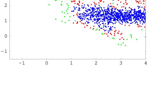
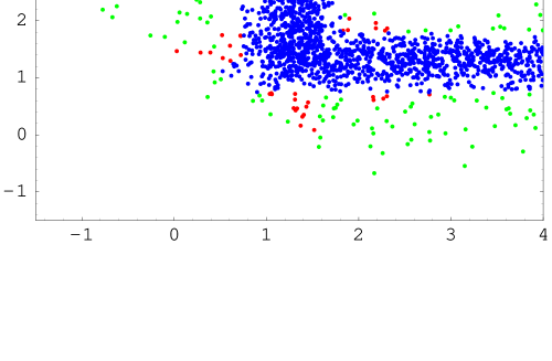
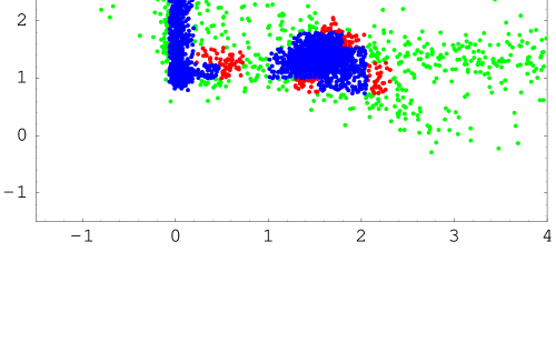
Figure 1: The exponent t₁₂ (vertical axis) versus t₁₁, t₁₃ and t₂₂.

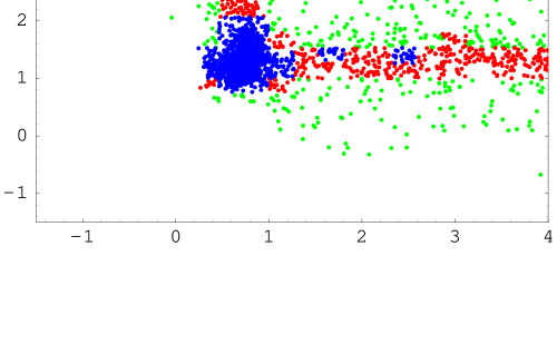
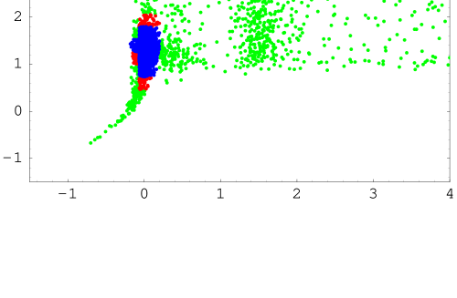
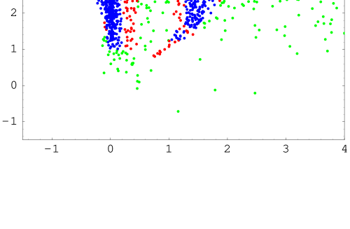
Figure 2: The exponent $t_{12}$ (vertical axis) versus $t_{23}$, $t_{33}$ and in the third figure the exponent $t_{11}$ (vertical axis) versus $t_{33}$.

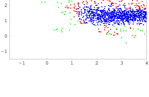
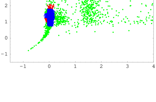
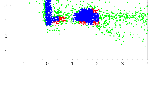
Figure 3: The exponent $t_{13}$ (vertical axis) vs $t_{11}$, $t_{22}$ and $t_{33}$.

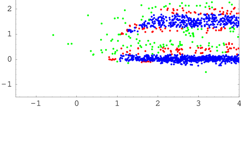
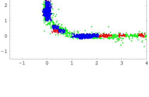
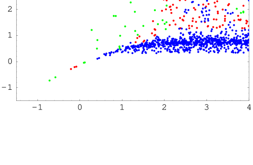
Figure 4: The exponent t₂₂ (vertical axis) vs $t_{11}$, $t_{33}$ and in the last figure the exponent $t_{23}$ vs $t_{11}$.

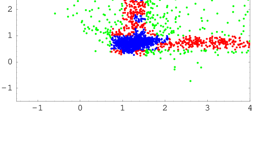
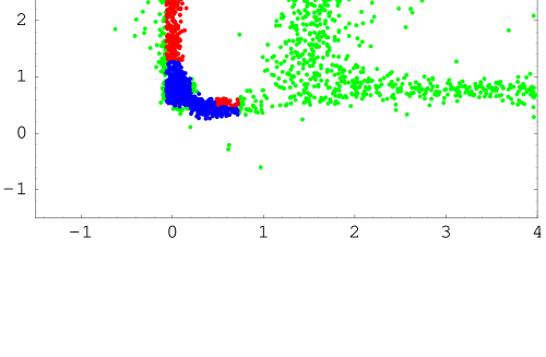
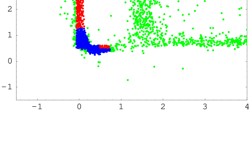
Figure 5: The exponent $t_{23}$ (vertical axis) vs $t_{13}$, $t_{22}$ and $t_{33}$.

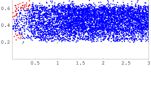
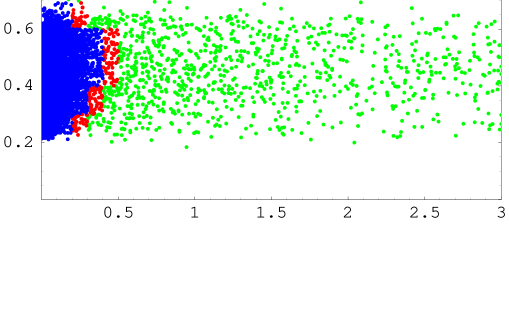
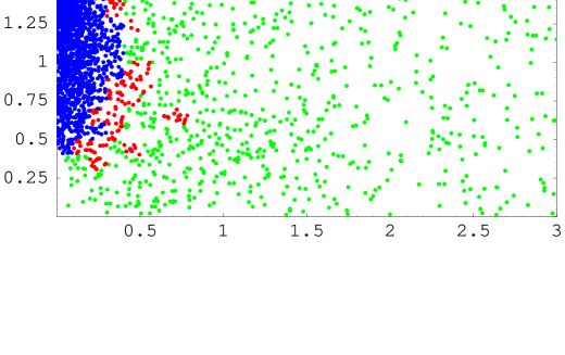
Figure 6: The exponent $p$ (vertical axis) vs $d$ and $r$ and, in the last figure, the exponent d (vertical axis) vs $r$.

References

- [1] F. Caravaglios, P. Roudeau and A. Stocchi, Nucl. Phys. B 633 (2002) 193 [arXiv:hep-ph/0202055].
- [2] S. M. Bilenky, arXiv:hep-ph/0205047, talk given at the XVI Rencontres de Physique de la Vallee d’Aoste, La Thuile, Italy, March 2002 ; P. Aliani, V. Antonelli, R. Ferrari, M. Picariello and E. Torrente-Lujan, arXiv:hep-ph/0206308.
- [3] G. Altarelli and F. Feruglio, arXiv:hep-ph/0206077;
- [4] M. Frigerio and A. Y. Smirnov, arXiv:hep-ph/0207366; E. Ma, arXiv:hep-ph/0207352.
- [5] O. Kofoed-Hansen, Phys. Rev. 71, 451 (1947); G. C. Hanna and B. Pontecorvo, Phys. Rev. 75, 451 (1949)
-
[6]
R. Barate et al., Eur. Phys. J. C2, 395
(1998); see also:
J. M. Roney, Nucl. Phys. Proc. Suppl. 91, 287 (2001) D. E. Groom et al., Eur. Phys. J. C15, 1 (2000) - [7] H. V. Klapdor-Kleingrothaus et al., Eur. Phys. J. A 12, 147 (2001).
- [8] C. E. Aalseth et al. [IGEX Collaboration], Phys. Rev. D 65, 092007 (2002)
- [9] J. Bonn et al., Nucl. Phys. Proc. Suppl. 91, 273 (2001); Ch. Weinheimer et al., Phys. Lett. B460, 219 (1999)
- [10] V. M. Lobashev et al., Nucl. Phys. Proc. Suppl. 91, 280 (2001); V. M. Lobashev et al., Phys. Lett. B460 (1999)
- [11] A. Osipowicz et al, KATRIN letter of intent, arXiv:hep-ex/0109033
- [12] S. Pascoli and S. T. Petcov, arXiv:hep-ph/0111203; F. Vissani, Nucl. Phys. Proc. Suppl. 100 (2001) 273 [arXiv:hep-ph/0012018]; F. Vissani, JHEP 9906 (1999) 022 [arXiv:hep-ph/9906525].
- [13] H. V. Klapdor-Kleingrothaus, A. Dietz, H. L. Harney and I. V. Krivosheina, Mod. Phys. Lett. A 16, 2409 (2001)
- [14] F. Feruglio, A. Strumia and F. Vissani, Nucl. Phys. B 637 (2002) 345 [arXiv:hep-ph/0201291].
- [15] B. T. Cleveland et al, Astrophys. J. 496, 505 (1998)
- [16] SAGE collaboration, J. N. Abdurashitov et al, Phys. Rev. C 60 055801 (1999) ; J. N. Abdurashitov et al. [SAGE Collaboration], arXiv:astro-ph/0204245.
- [17] GALLEX collaboration, W. Hampel et al, Phys. Lett. B 447, 127 (1999)
- [18] GNO collaboration, M. Altmann et al, Phys. Lett. B 490, 16 (2000); GNO collaboration, E. Bellotti et al, First Results from GNO, in Neutrino 2000, Proc. of the XIXth International Conference on Neutrino Physics and Astrophysics, Nucl. Phys. B91 Proc. Suppl., 44 (2001)
- [19] Kamiokande collaboration, Y. Fukuda et al, Phys. Rev. Lett. 77, 1683 (1996)
- [20] Super-Kamiokande collaboration, S. Fukuda et al, Phys. Rev. Lett. 86, 5651 (2001); S. Fukuda et al. [Super-Kamiokande Collaboration], Phys. Lett. B 539, 179 (2002) [arXiv:hep-ex/0205075]. M. B. Smy, arXiv:hep-ex/0206016.
- [21] SNO collaboration, Q. R. Ahmad et al, Phys. Rev. Lett. 87, 071301 (2001)
- [22] Q. R. Ahmad et al. [SNO Collaboration], Phys. Rev. Lett. 89 (2002) 011301 [arXiv:nucl-ex/0204008].
- [23] Q. R. Ahmad et al. [SNO Collaboration], Phys. Rev. Lett. 89 (2002) 011302 [arXiv:nucl-ex/0204009].
- [24] J. N. Bahcall, M. C. Gonzalez-Garcia and C. Pena-Garay, JHEP 0207 (2002) 054 [arXiv:hep-ph/0204314]; S. Pascoli and S. T. Petcov, Phys. Lett. B 544 (2002) 239 [arXiv:hep-ph/0205022]; P. Aliani, V. Antonelli, R. Ferrari, M. Picariello and E. Torrente-Lujan, arXiv:hep-ph/0205053; P. Aliani, V. Antonelli, M. Picariello and E. Torrente-Lujan, arXiv:hep-ph/0207348; P. Aliani, V. Antonelli, M. Picariello and E. Torrente-Lujan, Nucl. Phys. B 634 (2002) 393 [arXiv:hep-ph/0111418]; V. Barger, D. Marfatia, K. Whisnant and B. P. Wood, Phys. Lett. B 537 (2002) 179 [arXiv:hep-ph/0204253]. A. Bandyopadhyay, S. Choubey, S. Goswami and D. P. Roy, Phys. Lett. B 540 (2002) 14 [arXiv:hep-ph/0204286]; R. Foot and R. R. Volkas, Phys. Lett. B 543 (2002) 38 [arXiv:hep-ph/0204265]; P. C. de Holanda and A. Y. Smirnov, arXiv:hep-ph/0205241; A. Strumia, C. Cattadori, N. Ferrari and F. Vissani, Phys. Lett. B 541 (2002) 327 [arXiv:hep-ph/0205261].
- [25] K. S. Hirata et al. [Kamiokande-II Collaboration], Phys. Lett. B 280, 146 (1992).
- [26] Y. Fukuda et al. [Super-Kamiokande Collaboration] Phys. Rev. Lett. 81, 1562 (1998); T. Toshito [SuperKamiokande Collaboration] arXiv:hep-ex/0105023.
- [27] M. Shiozawa, for the Super-Kamiokande collaboration, talk given at Neutrino 2002, XXth International Conference on Neutrino Physics and Astrophysics, May 2002, Munich
- [28] R. Becker-Szendy et al., Nucl. Phys. Proc. Suppl. 38, 331 (1995).
- [29] M. Sanchez [Soudan-2 Collaboration], Int. J. Mod. Phys. A 16S1B, 727 (2001).
- [30] M. Ambrosio et al. [MACRO Collaboration], arXiv:hep-ex/0206027.
- [31] M. Sung, Int. J. Mod. Phys. A 16S1B, 752 (2001); C. Athanassopoulos et al. [LSND Collaboration], Phys. Rev. Lett. 81 (1998) 1774
- [32] J. Wolf [KARMEN Collaboration], “Final LSND and KARMEN-2 neutrino oscillation results”, Published in *Budapest 2001, High energy physics* hep2001/301; K. Eitel et al. [KARMEN collaboration], Nucl. Phys. Proc. Suppl. 77 (1999) 212
- [33] G. Drexlin, talk given at Neutrino 2002, XXth International Conference on Neutrino Physics and Astrophysics, May 2002, Munich
- [34] E. A. Hawker, Int. J. Mod. Phys. A 16S1B, 755 (2001); R. Stefanski [MINIBOONE Collaboration], Nucl. Phys. Proc. Suppl. 110, 420 (2002).
- [35] R. J. Wilkes [K2K Collaboration], “Results from K2K”, Published in Venice 2001, Neutrino telescopes, vol. 1 179-190; C. Yanagisawa, Nucl. Phys. Proc. Suppl. 95, 130 (2001); K. Nishikawa, for the K2K collaboration, talk given at Neutrino 2002, XXth International Conference on Neutrino Physics and Astrophysics, May 2002, Munich
- [36] S. Katsanevas, “The CNGS program status and Physics potential”, talk given at Neutrino 2002, XXth International Conference on Neutrino Physics and Astrophysics, May 2002, Munich; A. Weber [MINOS and OPERA Collaborations], “Status of the LBL oscillation experiments MINOS and OPERA”; Published in *Budapest 2001, High energy physics* hep2001/194; J. Rico [ICARUS Collaboration], arXiv:hep-ex/0205028; F. Arneodo et al., Nucl. Instrum. Meth. A 461, 324 (2001).
- [37] V. Paolone, Nucl. Phys. Proc. Suppl. 100, 197 (2001); K. Lang [MINOS Collaboration], Nucl. Instrum. Meth. A 461, 290 (2001); T. Ota and J. Sato, arXiv:hep-ph/0202145; V. D. Barger, A. M. Gago, D. Marfatia, W. J. Teves, B. P. Wood and R. Zukanovich Funchal, Phys. Rev. D 65, 053016 (2002)
- [38] M. Apollonio et al., CHOOZ Coll., Phys. Lett. B 466, 415 (1999)
- [39] Y. F. Wang [Palo Verde Collaboration], Int. J. Mod. Phys. A 16S1B, 739 (2001); F. Boehm et al., Phys. Rev. D 64, 112001 (2001)
- [40] G. Altarelli and F. Feruglio, Phys. Lett. B 451 (1999) 388; G. Altarelli, F. Feruglio and I. Masina, JHEP 0011 (2000) 040; P.Binetruy and P.Ramond, Phys. Lett. B 350 (1995) 49; P. Binetruy, S. Lavignac and P. Ramond, Nucl. Phys. B 477 (1996) 353; E. Dudas, S. Pokorski and C. A. Savoy, Phys. Lett. B 369 (1996) 255; Q. Shafi and Z. Tavartkiladze, Phys. Lett. B 482 (2000) 145; J. M. Mira, E. Nardi and D. A. Restrepo, Phys. Rev. D 62 (2000) 016002; A. E. Nelson and D. Wright, Phys. Rev. D 56 (1997) 1598; V. Jain and R. Shrock, Phys. Lett. B 352, 83 (1995); W. Buchmuller and M. Plumacher, Int. J. Mod. Phys. A 15, 5047 (2000); W. Buchmuller and D. Wyler, Phys. Lett. B 521, 291 (2001).
- [41] R. Barbieri, L. J. Hall and A. Romanino, Nucl. Phys. B551 (1999) 93 and references therein; Z. G. Berezhiani, Phys. Lett. B 150 (1985) 177; R. Barbieri, G. R. Dvali and L. J. Hall, Phys. Lett. B 377 (1996) 76; A. Pomarol and D. Tommasini, Nucl. Phys. B 466 (1996) 3 K. S. Babu and R. N. Mohapatra, Phys. Rev. Lett. 83 (1999) 2522 P. Pouliot and N. Seiberg, Phys. Lett. B 318, 169 (1993); R. Kitano and Y. Mimura, Phys. Rev. D 63, 016008 (2001)
- [42] P. H. Frampton and O. C. Kong, Phys. Rev. Lett. 77 (1996) 1699; P. H. Frampton and A. Rasin, Phys. Lett. B 478 (2000) 424; A. Aranda, C. D. Carone and P. Meade, Phys. Rev. D 65, 013011 (2002); A. Aranda, C. D. Carone and R. F. Lebed, Phys. Rev. D 62, 016009 (2000); D. B. Kaplan and M. Schmaltz, Phys. Rev. D 49, 3741 (1994); K. S. Babu, E. Ma and J. W. Valle, arXiv:hep-ph/0206292.
- [43] C. A. Lee, Q. Shafi and Z. Tavartkiladze, arXiv:hep-ph/0206258; A. Lukas, P. Ramond, A. Romanino and G. G. Ross, Phys. Lett. B 495 (2000) 136; R. Barbieri, P. Creminelli and A. Strumia, Nucl. Phys. B 585 (2000) 28; D. O. Caldwell, R. N. Mohapatra and S. J. Yellin, Phys. Rev. D 64 (2001) 073001; A. Lukas, P. Ramond, A. Romanino and G. G. Ross, JHEP 0104 (2001) 010; A. De Gouvea, G. F. Giudice, A. Strumia and K. Tobe, Nucl. Phys. B 623 (2002) 395; A. S. Dighe and A. S. Joshipura, Phys. Rev. D 64 (2001) 073012; H. Davoudiasl, P. Langacker and M. Perelstein, Phys. Rev. D 65, 105015 (2002); K. Benakli and A. Y. Smirnov, Phys. Rev. Lett. 79, 4314 (1997); N. Arkani-Hamed, S. Dimopoulos, G. R. Dvali and J. March-Russell, Phys. Rev. D 65, 024032 (2002); N. Arkani-Hamed, S. Dimopoulos and G. R. Dvali, Phys. Lett. B 429, 263 (1998); A. E. Faraggi and M. Pospelov, Phys. Lett. B 458 (1999) 237; K. R. Dienes, E. Dudas and T. Gherghetta, Nucl. Phys. B 557 (1999) 25; G. R. Dvali and A. Y. Smirnov, Nucl. Phys. B 563 (1999) 63; Y. Grossman and M. Neubert, Phys. Lett. B 474 (2000) 361; R. N. Mohapatra and A. Perez-Lorenzana, Nucl. Phys. B 576 (2000) 466.
- [44] S. Antusch, M. Drees, J. Kersten, M. Lindner and M. Ratz, Phys. Lett. B 519, 238 (2001); J. A. Casas, J. R. Espinosa, A. Ibarra and I. Navarro, Nucl. Phys. B 573, 652 (2000).
- [45] M. Hirsch, arXiv:hep-ph/0102102; M. S. Berger and K. Siyeon, Phys. Rev. D 63, 057302 (2001). L. J. Hall, H. Murayama and N. Weiner, Phys. Rev. Lett. 84, 2572 (2000).
- [46] F. Vissani, Phys. Lett. B 508, 79 (2001).