IFUM-560/FT
FTUAM-02-387
KamLAND potentiality on the determination of Neutrino mixing parameters in the post SNO-NC era
P. Aliania⋆, V. Antonellia⋆, M. Picarielloa⋆, E. Torrente-Lujanab⋆
a Dip. di Fisica, Univ. di Milano,
and INFN Sez. Milano, Via Celoria 16, Milano, Italy
b Dept. Fisica Teorica C-XI,
Univ. Autonoma de Madrid, 28049 Madrid, Spain,
Abstract
We study in detail the power of the reactor experiment KamLAND for discriminating existing solutions to the SNP and giving accurate information on neutrino masses and mixing angles. Assuming the expected signal corresponding to various “benchmark” points in the 2 dimensional mixing plane, we develop a full-fledged analysis which include KamLAND spectrum and all the existing solar evidence. A complete modelling of statistical and known systematics errors for 1 and 3 years of data taking is included, exclusion plots are presented.
We find a much higher sensitivity especially for values of lying in the central part of the LMA region. The situation would be more complicate for values closer to the border of the LMA region (the so called HLMA region, i.e. and or far from ). In this case kamLAND, with or without solar evidence, will only be able to select multiple regions in the parameter space, in the sense that different possible values of the parameters would produce the same signal.
PACS:
⋆ e-mail: paola.aliani@cern.ch, vito.antonelli@mi.infn.it, marco.picariello@mi.infn.it, emilio.torrente-lujan@cern.ch
1 Introduction
The publication of the recent SNO results [1, 2, 3] has made an important breakthrough towards the solution of the long standing solar neutrino [14, 35, 36, 37, 39, 40, 38, 41, 42] problem (SNP) possible. These results provide the strongest evidence so far for flavor oscillation in the neutral lepton sector.
In the near future the reactor experiment KamLAND [4, 5] is expected to further improve our knowledge of neutrino mixing. In fact it should be able to sound the region of the mixing parameter space corresponding to the so called Large Mixing Angle (LMA) solution of the solar neutrino problem ( and ) more profoundly. This is of prime interest due to the fact that the LMA region in the one preferred by the solar neutrino data at present.
The previous generation of reactor experiments (CHOOZ [6], PaloVerde [8]), performed with a baseline of about 1 km. They have attained a sensitivity of [7, 6] and, not finding any dissapearence of the initial flux, they demonstrated that the atmospheric neutrino anomaly [11] is not due to muon-electron neutrino oscillations. The KamLAND experiment is the successor of such experiments at a much larger scale in terms of baseline distance and total incident flux.
This experiment relies upon a 1 kton liquid scintillator detector located at the old, enlarged, Kamiokande site. It searches for the oscillation of antineutrinos emitted by several nuclear power plants in Japan. The nearby 16 (of a total of 51) nuclear power stations deliver a flux of for neutrino energies MeV at the detector position. About of this flux comes from 6 reactors forming a well defined baseline of 139-214 km. Thus, the flight range is limited in spite of using several reactors, because of this fact the sensitivity of KamLAND will increase by nearly two orders of magnitude compared to previous reactor experiments.
It has been estimated that even in the most conservative scenario [4], in which the background has to be determined from the reactor power fluctuations, the LMA solution is completely within the estimated sensitivity after 3 years of data taking. Moreover, KamLAND should be able [4] to determine the mixing angle and mass difference with a accuracy at 99% of confidence level (CL). As has been underlined in [12] and later in [13], the problems might arise if the value of the squared mass difference () lies in the upper region of the LMA solution, the so called HLMA region.
Let us briefly recall some model independent conclusions obtained from the results of SNO [14]. Different quantities can be defined in order to make the evidence for disappearance and appearance of the neutrino flavors explicit. Letting alone the SNO data, from the three fluxes measured by SNO is possible to define two useful ratios: , , deviations of these ratios with respect to their standard value are powerful tests for occurrence of new physics. For the first ratio, one obtains [14]
a value which is 2.7 away from the no-oscillation expectation value of one. The ratio of CC and NC fluxes gives the fraction of electron neutrinos remaining in the solar neutrino beam, the value obtained in Ref. [14]:
this value is far away from the standard model case.
Finally, if in addition to SNO data one consider the flux predicted by the solar standard mode one can define, following Ref.[16], the quantity , the fraction of ” neutrinos which oscillated into active ones”, one finds the following result:
where the SSM flux is taken as the flux predicted in Ref.[17]. The central value is clearly below one (only-active oscillations). Although electron neutrinos are still allowed to oscillate into sterile neutrinos the hypothesis of transitions to only sterile neutrinos is rejected at nearly .
The aim of this work is to study the KamLAND discriminating power, to understand in which regions of the parameter space still allowed by the solar neutrino experiments KamLAND might give satisfactory accuracy. The structure of this work is the following. In section 2 we discuss the main features of KamLAND experiment that are relevant for our analysis: we derive updated numerical expressions for the reactor fuel cycle-averaged antineutrino flux and the absortion antineutrino cross section. The next section is devoted to the salient aspects of the procedure we are adopting. The results of our analysis are presented and discussed in section 4 and, finally, in section 5 we draw our conclusions and discuss possible future scenarios.
2 A Kamland overview
Electron antineutrinos from nuclear reactors with energies above 1.8 MeV are measured in KamLAND by detecting the inverse -decay reaction . The time coincidence, the space correlation and the energy balance between the positron signal and the 2.2 MeV -ray produced by the capture of a already-thermalized neutron on a free proton make it possible to identify this reaction unambiguously, even in the presence of a rather large background.
The two principal ingredients in the calculation of the expected signal in KamLAND are the reactor flux and the antineutrino cross section on protons. These ingredients are considered below.
2.1 The reactor antineutrino flux
We first describe the flux of antineutrinos coming from the power reactors. A number of short baseline experiments ( Ref.[18] and references therein) have measured the energy spectrum of reactors at distances where oscillatory effects have been shown to be inexistent. They have shown that the theoretical neutrino flux predictions are reliable within 2% [4].
The effective flux of antineutrinos released by the nuclear plants is a rather well understood function of the thermal power of the reactor and the amount of thermal power emitted during the fission of a given nucleus, which gives the total amount, and the isotopic composition of the reactor fuel which gives the spectral shape. Detailed tables for these magnitudes can be found in Ref. [18].
For a given isotope the energy spectrum can be parametrized by the following expression [19]
| (1) |
where the coefficients depend on the nature of the fissionable isotope (see Ref.[18] for explicit values). Along the year, between periods of refueling, the total effective flux changes with time as the fuel is expended and the isotope relative composition varies. The overall spectrum is at a given time
To compute a fuel-cycle averaged spectrum we have made use of the typical evolution of the relative abundances , which can be seen in Fig. 2 of Ref.[18]. This averaged spectrum can be again fitted very well by the same functional expression (1). The isotopic energy yield is properly taken into account. As the result of this fit, we obtain the following values which are the ones to be used in the rest of this work:
Although individual variations of the along the fuel cycle can be very high, the variation of the two most important ones is highly correlated: the coefficient increases in the range while decreases . This correlation makes the effective description of the total spectrum by a single expression Eq.1 useful. With the fitted coefficients above, the difference between this effective spectrum and the real one is typically along the yearly fuel cycle.
2.2 Antineutrino cross sections
We now consider the cross sections for antineutrinos on protons. We will sketch the form of the well known differential expression and more importantly we will give updated numerical values for the transition matrix elements which appear as coefficients.
In the limit of infinite nucleon mass, the cross section for the reaction is given by [20, 21] where are the positron energy and momentum and a transition matrix element which will be considered below. The positron spectrum is monoenergetic: and are related by: , where are the neutron and proton masses and MeV.
Nucleon recoil corrections are potentially important in relating the positron and antineutrino energies in order to evaluate the antineutrino flux. Because the antineutrino flux would typically decrease quite rapidly with energy, the lack of adequate corrections will systematically overestimate the positron yield.
At highest orders, the positron spectrum is not monoenergetic and one has to integrate over the positron angular distribution to obtain the positron yield. The differential cross section at first order is of the form:
Complete expressions and notation can be found in Ref. [19]. Here we only want to pay attention to the overall coefficient which is related to the transition matrix element above.
The matrix transition element can be written in terms of measurable quantities as
where appears the free neutron decay , the phase-space factor f and . The value of follows from calculation [22], while sec is the latest published value for the neutron half-life [23]. This value has a significantly smaller error than previously quoted measurements.
From the values above, we obtain the extremely precise value:
From here the coefficient which appears in the differential cross section is obtained as (vector and axial vector couplings ): In summary, the differential cross section which appear in KamLAND are very well known, its theoretical errors are negligible if updated values are employed.
3 The computation of the expected signals
In order to obtain the expected number of events at KamLAND, we sum the expectations for all the relevant reactor sources weighting each source by its power and distance to the detector (table II in Ref. [18] ), assuming the same spectrum originated from each reactor. The average number of positrons which are detected per visible energy bin is given by the convolution of different quantities: , the oscillation probability averaged over the distance and power of the different reactors, the antineutrino capture cross section given as before, the antineutrino flux spectrum given by expression 1, the relative reactor-reactor power normalization which is included in the definition of and the energy resolution of KamLAND which is rather good [5], we use in our analysis the expression .
For one year of running with the 600 ton fiducial mass and for standard nuclear plant power and fuel schedule: we assume all the reactors operated at of their maximum capacity and an averaged, time-independent, fuel composition equal for each detector, the experiment expects about 550 antineutrino events (this number agrees with other estimations. i.e. Ref.[5]). We will consider this number as our KamLAND year in what follows. We will not add any background events as we will suppose that they can be distinguished from the signal with sufficiently high efficiency. This should be taken with caution, we will dedicate a few words to the experimental background at the end of section.
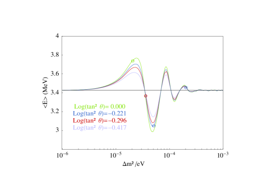
We compute the expected signal in a set of 0.5 MeV width total positron energy bins in the range 2.0 MeV - 8 MeV. Quantitavely, the main information content of the shape of the observable spectrum is summarized by the first moment of the distribution, the average spectrum energy. This first moment is defined as
| (2) |
where is the center positron energy in the i energy bin and the normalized signals relative to the non-oscillation case: .
The expected value of this first moment as a function of for some selected values of the mixing angle is represented in Fig. 1(right). We want to illustrate the potentiality of this magnitude as an indicator of neutrino oscillations at KamLAND. In this plot we graphically see the fact that KamLAND is sensitive to neutrino oscillations in the LMA region and in particular to the parameter. The first moment can vary up in sizeable regions of the parameter space (this can be beautifully seen in a 3D plot). A variation of a fraction of this size should be clearly identifiable from the KamLAND data after 1 year of effective running. In order to see whether this result depends on the choice of bin-size, we have also reproduced it with larger, 1 MeV bins, and found that there is no significant difference.
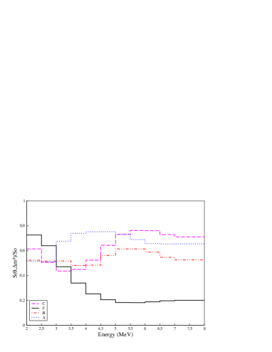
In Fig.1 (left) we show the visible positron energy spectrum at KamLAND for some chosen oscillation parameters (see Table 1). We present the integrated signal at every 0.5 MeV bin normalized to the non-oscillation expectation. We can see from the plot how the shape of the signal is very sensitive to the oscillation parameters. It can greatly change through the LMA region. From the point of view of background reduction, in some favorable cases the spectrum is peaked above 5 MeV, this suggests the extension of the fiducial energy thresholds beyond the 8 MeV level.
The random coincidence background is due to the contamination of the detector scintillator by U, Th and Rn. From MC studies and assuming that an adequate level of purification can be obtained, the background coming from this source is expected to be events/d/kt which is equivalent to a signal to background ratio of . Other works [10] conservatively estimate a level for this ratio. More importantly for what it follows, one expects that the random coincidence backgrounds will be a relatively steeply falling function of energy. The assumption of no background should be relatively safe only at high energies (above MeV).
The second source of background, the so called correlated background is dominantly caused by cosmic ray muons and neutrons. The KamLAND’s depth is the main tool to suppress those backgrounds. MC methods estimate a correlated background of around events/day/kt distributed over all the energy range up to MeV.
We will also need the expected signals in the different solar neutrino experiments. These are obtained by convoluting solar neutrino fluxes, sun and earth oscillation probabilities, neutrino cross sections and detector energy response functions. We closely follow the same methods already well explained in previous works [24, 25, 14, 26], we will mention here only a few aspects of this computation. We determine the neutrino oscillation probabilities using the standard methods found in literature [27], as explained in detail in [24] and in [14]. We use a thoroughly numerical method to calculate the neutrino evolution equations in the presence of matter for all the parameter space. For the solar neutrino case the calculation is split in three steps, corresponding to the neutrino propagation inside the Sun, in the vacuum (where the propagation is computed analytically) and in the Earth. We average over the neutrino production point inside the Sun and we take the electron number density in the Sun by the BPB2001 model [17]. The averaging over the annual variation of the orbit is also exactly performed. To take the Earth matter effects into account, we adopt a spherical model of the Earth density and chemical composition [28]. The gluing of the neutrino propagation in the three different regions is performed exactly using an evolution operator formalism [27]. The final survival probabilities are obtained from the corresponding (non-pure) density matrices built from the evolution operators in each of these three regions.
In this analysis in addition to night probabilities we will need the partial night probabilities corresponding to the 6 zenith angle bin data presented by SK [43]. They are obtained using appropriate weights which depend on the neutrino impact parameter and the sagitta distance from neutrino trajectory to the Earth’s center, for each detector’s geographical location.
4 Analysis and Results
In order to study the potentiality of KamLAND for resolving the neutrino oscillation parameter space, we have developed two kind of analysis. In the first case (Analysis A below) we will deal with the KamLAND expected global signal. We will asumme that the experiment measure a certain global signal with given statistical and systematic error after some period of data taking (1 or 3 yrs) and will perform a complete statistical analysis including in addition the up-date solar evidence. In the second case, Analysis B, we will include the full KamLAND spectrum information. Instead of giving arbitrary values to the different bins, we will assume a number of oscillation models characterized by their mixing parameters . After including the solar evidence we will perform the same analysis as before.
4.1 Analysis A
The total value is given by the sum of two distinct contributions, that is the one coming from all the solar neutrino data and the contribution of the KamLAND experiment:
with
| (3) |
For the “experimental” signal ratio we assume different values varying from a very strong suppression to unobservation of neutrino oscillations . The total error is computed as a sum of assumed systematics deviations, , mainly coming from flux uncertainty (), energy baseline calibration and others (see Ref.[klsystematics, Murayama:2000qi, 5]) and statistical errors . The nominal periods of data taking that we consider, 1 and 3 yrs, are generical representative cases where systematical or statistical errors are taken as predominant.
The solar neutrino contribution can be written in the following way:
| (4) |
The function correspond to the total event rates measured at the Homestake experiment [29] and at the gallium experiments SAGE [30, 31], GNO [32] and GALLEX [33]. We follow closely the definition used in previous works (see Ref.[14] for definitions and Table (1) in Ref.[14] ‘ for an explicit list of results and other references).
The contribution to the from the SuperKamiokande data () has been obtained by using double-binned data in energy and zenith angle (see table 2 in Ref.[43] and also Ref.[34]): 8 energy bins of variable width and 7 zenith angle bins which include the day bin and 6 night ones. The definition is given by:
| (5) |
The theoretical and experimental quantities are this time matrices of dimension 87. The factor is a flux normalization with respect to the value measured by SNO NC. The covariance quantity is a 4-rank tensor constructed in terms of statistic errors, energy and zenith angle bin-correlated and uncorrelated uncertainties. The data and errors for individual energy bins for SK spectrum has been obtained from Ref. [43].
The contribution of SNO to the is given by
| (6) |
The presence of the first term is due to the introduction in our analysis of the flux normalization factor with respect to the SNO NC flux, whose central and error values are given in Table I of Ref.[14]. The second term in formula 6 corresponds to:
| (7) |
where the day and night vectors of dimension 17 are made up by the values of the total (NC+CC+ES) SNO signal for the different bins of the spectrum. The statistical contribution to the covariance matrix, , is obtained directly from the SNO data. The part of the matrix related to the systematical errors has been computed by us studying the influence on the response function of the different sources of correlated and uncorrelated errors reported by SNO collaboration (see table II of Ref. [2]), we assume full correlation or full anticorrelation according to each source.
To test a particular oscillation hypothesis against the parameters of the best fit and obtain allowed regions in parameter space we perform a minimization of the three dimensional function . For , a given point in the oscillation parameter space is allowed if the globally subtracted quantity fulfills the condition . Where are the quantiles for three degrees of freedom.
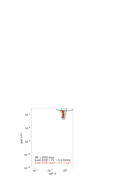
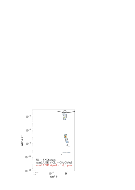
In Fig.2 we graphically show the results of this analysis. They represent exclusion plots including KamLAND global rates, given a hypothetical experimental global signal ratio: respectively strong and medium suppression and no oscillation evidence for one and three years of KamLAND data taking. As can be seen in the figures, as the KamLAND experimental signal decreases, the LMA region is singled out. The periodic shape in of the 90 % C.L. (red regions) which becomes apparent in the three-year plot is due to the periodicity of the response function: in order to distinguish among these different equally-likely solutions, one must analyze the energy spectrum, this will done in the main analysis to be presented in the next sections. Obviously, only if KamLAND sees some oscillation signal (i.e. ) does the LMA region become the only solution. If we consider a hypothetical signal closer to 1.0 than 0.3, we see that the LOW region survives, although it is less favored.
4.2 Analysis B
Here we use the expected binned KamLAND signal for some benchmark, arbitrarily chosen, points in parameter space that we show in table (1). For any of these points we obtain the expected spectrum after 1 or 3 years of data taking under the “standard” conditions described above. Next we perform an standard analysis introducing statistical and assumed systematics errors including the evidence of the up-date solar experiments (CL,GA,SK and SNO).
In the present study the total value is given by the sum of two distinct contributions, that is the one coming from all the solar neutrino data and the contribution of the KamLAND experiment:
| (8) |
The contribution of the solar neutrino experiments is described in detail in the previous section. The contribution of the KamLAND experiment is now as follows:
| (9) |
Note that the addition to of a constant term has no practical importance for the main purpose of this kind of analysis: the determination of exclusion regions proceeds from the minimum subtracted quantity . The are length 12 vectors containing the binned spectrum (0.5 MeV bins ranging from 2 to 8 MeV) normalized to the non-oscillation expectations. Theoretical vectors are a function of the oscillation parameters: . The “experimental” vectors are defined in similar way, for any of the benchmark points we have .
We generate acceptance contours (at 90,95 and 99 % CL) in the plane in a similar manner as explained in the previous section. For the sake of comparison we have also obtained exclusion regions derived from the consideration of the alone.
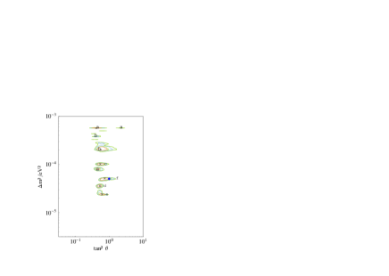
In Figs.(3) we graphically show the results of this analysis for a selection of points and for three years of data taking restricting ourselves to the LMA region of the parameter space where, as we have noted before, the KamLAND spectrum information is specially significative. In each plot allowed regions corresponding to different starting points are superimposed, every region is distinguished with a label. The position of initial points is labeled with solid stars.
The first case, study of the KL spectrum alone () is represented by the Fig.(3 left). The allowed parameter space corresponding to each particular point is formed by a number of, highly degenerated, disconnected regions symmetric with respect the line . These regions can extend very far from the initial point specially in terms of but also in some occasions in terms of . For example the point “A” located at gives rise to two sets of thin regions situated respectively at and a third region situated at which practically covers the full range . A similar behavior is observed for point “B”. Of course this situation is not very favorable for the future phenomenologist trying to extract conclusions from the KamLAND data. A much comfortable situation is found for points nearer the center of the LMA region. Note how the regions corresponding to the points “D,E” and specially “F” only extend very gently around the initial location.
The results of the full analysis are summarized in Fig.(3, right). The position of the minima of , marked in the plot with crosses, is practically identical to the position of the initial points except in some case where the difference is not significant anyway. The general effect of the inclusion of the solar evidence in the is the breaking of the symmetry in as expected and the general reduction of the number of disconnected regions corresponding to each point. Note however that the point “A” still gives rise to a small allowed region situated nearly one order of magnitude smaller in . The “B” region is shrinked near its initial location as happens to the rest of points. The conclusion to be drawed from these plots is that KamLAND together with the rest of solar experiments will be able to resolve the neutrino mixing parameters with a precision of practically everywhere. However, for values of the problem of the coexistence of multiple regions with similar statistical significance will still be present.
5 Summary and Conclusions
We have analyzed the present experimental situation of our knowledge of the neutrino mixing parameters in the region of the parameter space that is relevant for solar neutrinos and we have studied in detail how this knowledge should improve with the forthcoming reactor experiment KamLAND.
In this work we have presented in some detail the characteristic of KamLAND experiment including antineutrino reactor fluxes and absortion cross sections for which we have given updated values. We find that present theoretical errors in this cross secion are negligible.
We have studied the expected KamLAND spectrum for different possible (“benchmark points”) values of the mixing parameters selected inside the LMA region. The shape of the spectrum shows a significant dependence on the values of the mixing parameters. The spectrum distortion caused by oscillation have been characterized by the first moment of the positron energy distribution. The results confirm that KamLAND is very sensitive to neutrino oscillation in the LMA region. In particular the value of the first moment changes very much for values of varying inside the region . The dependence on the value of the mixing angle is also evident, even if somehow milder. In the LOW and SMA region, instead, the value of the moment is essentially constant. We have also verified that the result doesn’t depend in a significant way on the choice of the bin size.
In order to investigate the discrimination power of KamLAND, we have selected different points (“benchmark points”) in the LMA region and studied which information KamLAND will be able to give after 1-3 years of running. We have included a full modelling of statistical and systematic uncertainties. The regions selected by KamLAND alone, all symmetric with respect to , have a large spreadth in the mixing angle. The experiment should have, instead, a much higher sensitivity to the mass difference parameter, especially for values of lying in the central part of the LMA region. The situation would be more complicate for values closer to the border of the LMA region or beyond already in the HLMA region (i.e. and or far from 0.5). In this case KamLAND, with or without solar evidence, will be able only to select multiple regions in the parameter space, in the sense that different possible values of the parameters would produce the same signal.
We have performed a similar analysis adding to the information from KamLAND would-be signal all the evidence already exististing on solar neutrinos. By using a analysis, we have produced exclusion plots. KamLAND will help to select the values of the mixing parameters especially in the case in which the solutions lies in the LMA region. If, instead, one moves towards values of the KamLAND signal closer to the no oscillation value (that at present seems to be strongly disfavored by the other experiments) the absolute minimum moves from the LMA to the LOW solution and one is left with small allowed regions not only in the LOW, but also in the SMA region. In summary, KamLAND together with the rest of solar experiments will be able to resolve the neutrino mixing parameters with a high precision practically everywhere. However, for values of (graphically emphatized by the two benchmark points labeled “A” and “B” in the plots) the problem of the coexistence of multiple regions with similar statistical significance will still be present.
Acknowledgments
It is a pleasure to thank R. Ferrari for many enlightening discussions and for his encouraging support. We acknowledge the financial support of the Italian MURST and the Spanish CYCIT funding agencies. One of us (E.T.) wish to acknowledge in addition the hospitality of the CERN Theoretical Division at the early stage of this work. P.A., V.A., and M.P. would like to thank the kind hospitaliy of the Dept. de Fisica Teorica of the U. Autonoma de Madrid. The numerical calculations have been performed in the computer farm of the Milano University theoretical group.
References
- [1] Q. R. Ahmad et al. [SNO Collaboration], Phys. Rev. Lett. 89, 011302 (2002) [arXiv:nucl-ex/0204009].
- [2] Q. R. Ahmad et al. [SNO Collaboration], Phys. Rev. Lett. 89, 011301 (2002) [arXiv:nucl-ex/0204008].
- [3] ’How to use recent SNO results’,http://www.sno.phy.queensu.ca/
- [4] A. Piepke [kamLAND collaboration], Nucl. Phys. Proc. Suppl. 91, 99 (2001)
- [5] J. Shirai, “Start of Kamland”, talk given at Neutrino 2002, XXth International Conference on Neutrino Physics and Astrophysics, May 2002, Munich. Transparencies can be obtained from http://neutrino2002.ph.tum.de. See also: P. Alivisatos et al., STANFORD-HEP-98-03.
- [6] M. Apollonio et al., CHOOZ Coll., Phys. Lett. B 466, 415 (1999)
- [7] M. Apollonio et al. (CHOOZ coll.), hep-ex/9907037, Phys. Lett. B 466 (1999) 415. M. Apollonio et al., Phys. Lett. B 420 (1998) 397. F. Boehm et al.,Phys. Rev. D62 (2000) 072002 [hep-ex/0003022].
- [8] Y. F. Wang [Palo Verde Collaboration], Int. J. Mod. Phys. A 16S1B, 739 (2001); F. Boehm et al., Phys. Rev. D 64, 112001 (2001) [arXiv:hep-ex/0107009].
- [9] L. De Braeckeleer [KamLAND Collaboration], Nucl. Phys. Proc. Suppl. 87 (2000) 312. J. Shirai, “Kamioka Liquid Scintillator Anti-Neutrino Detector”, Neutrino2002, May 25-30, Munich, Germany. A. Suzuki [KamLAND Collaboration], Nucl. Phys. Proc. Suppl. 77 (1999) 171.
- [10] . J. Busenitz et al. (US KamLand Coll). proposal for US Participation in KamLand. March 1999 (Unpublished).
- [11] K. S. Hirata et al. [Kamiokande-II Collaboration], Phys. Lett. B 280, 146 (1992). T. Toshito [SuperKamiokande Collaboration], arXiv:hep-ex/0105023; Y. Fukuda et al. [Super-Kamiokande Collaboration], Phys. Rev. Lett. 81, 1562 (1998) [arXiv:hep-ex/9807003]; R. Becker-Szendy et al., Nucl. Phys. Proc. Suppl. 38, 331 (1995); M. Sanchez [Soudan-2 Collaboration], Int. J. Mod. Phys. A 16S1B, 727 (2001); M. Ambrosio et al. [MACRO Collaboration], arXiv:hep-ex/0206027.
- [12] S. T. Petcov and M. Piai, Phys. Lett. B 533, 94 (2002) [arXiv:hep-ph/0112074].
- [13] S. Schonert, T. Lasserre and L. Oberauer, arXiv:hep-ex/0203013
- [14] P. Aliani, V. Antonelli, R. Ferrari, M. Picariello and E. Torrente-Lujan, arXiv:hep-ph/0205053.
- [15] J. N. Bahcall and E. Lisi, Phys. Rev. D 54, 5417 (1996) [arXiv:hep-ph/9607433].
- [16] V. Barger, D. Marfatia and K. Whisnant, arXiv:hep-ph/0106207.
- [17] J. N. Bahcall, M. H. Pinsonneault and S. Basu, Astrophys. J. 555, 990 (2001) [arXiv:astro-ph/0010346].
- [18] H. Murayama and A. Pierce, Phys. Rev. D 65 (2002) 013012 [arXiv:hep-ph/0012075].
- [19] P. Vogel, J.F. Beacom, hep-ph/9903554
- [20] G. Zacek et al. Phys. Rev. D34,9 (1986)2621.
- [21] F. Reines, R. M. Woods, Phys. Rev. Lett. 14 (1965) 20.
- [22] D. H. Wilkinson, Nucl. Phys. A377, 474 (1982).
- [23] K. Hagiwara et al., Phys. Rev. D 66 (2002) 010001
- [24] P. Aliani, V. Antonelli, M. Picariello and E. Torrente-Lujan, Nucl. Phys. B634 (2002) 693. arXiv:hep-ph/0111418.
- [25] P. Aliani, V. Antonelli, M. Picariello and E. Torrente-Lujan, Nucl. Phys. Proc. Suppl. 110, 361 (2002) [arXiv:hep-ph/0112101].
- [26] P. Aliani, V. Antonelli, R. Ferrari, M. Picariello and E. Torrente-Lujan, arXiv:hep-ph/0205061.
- [27] E. Torrente-Lujan, Phys. Rev. D 59 (1999) 093006. E. Torrente-Lujan, Phys. Rev. D 59 (1999) 073001. E. Torrente-Lujan, Phys. Lett. B 441 (1998) 305. V.B. Semikoz, E. Torrente-Lujan, Nucl. Phys. B 556 (1999) 353. E. Torrente-Lujan,Phys. Lett. B494 (2000) 255 [hep-ph/9911458].
- [28] I. Mocioiu and R. Shrock, Phys. Rev. D 62 (2000) 053017 [arXiv:hep-ph/0002149].
- [29] R. Davis, Prog. Part. Nucl. Phys. 32 (1994) 13; B.T. Cleveland et al., (HOMESTAKE Coll.) Nucl. Phys. (Proc. Suppl.)B 38 (1995) 47; B.T. Cleveland et al., (HOMESTAKE Coll.) Astrophys. J. 496 (1998) 505-526; K. Lande (For the Homestake Coll.) Nucl. Phys. B(Proc. Suppl.)77(1999)13-19.
- [30] A.I. Abazov et al. (SAGE Coll.), Phys. Rev. Lett. 67 (1991) 3332; D.N. Abdurashitov et al. (SAGE Coll.), Phys. Rev. Lett. 77 (1996) 4708; J.N. Abdurashitov et al., (SAGE Coll.), Phys. Rev. C60 (1999) 055801; astro-ph/9907131; J.N. Abdurashitov et al., (SAGE Coll.), Phys. Rev. Lett. 83 (1999) 4686; astro-ph/9907113. J. N. Abdurashitov et al. [SAGE Collaboration], of solar activity,” arXiv:astro-ph/0204245.
- [31] J.N. Abdurashitov et al. (SAGE Coll.) Phys. Rev. Lett. 83(23) (1999)4686.
- [32] M. Altmann et al. (GNO Coll.) Phys. Lett. B490 (2000) 16-26.
- [33] P. Anselmann et al., GALLEX Coll., Phys. Lett. B 285 (1992) 376; W. Hampel et al., GALLEX Coll., Phys. Lett. B 388 (1996) 384; T.A. Kirsten, Prog. Part. Nucl. Phys. 40 (1998) 85-99; W. Hampel et al., (GALLEX Coll.) Phys. Lett. B 447 (1999) 127; M. Cribier, Nucl. Phys. (Proc. Suppl.)B 70 (1999) 284; W. Hampel et al., (GALLEX Coll.) Phys. Lett. B 436 (1998) 158; W. Hampel et al., (GALLEX Coll.) Phys. Lett. B 447 (1999) 127.
- [34] S. Fukuda et al. [Super-Kamiokande Collaboration], Phys. Lett. B 539, 179 (2002) [arXiv:hep-ex/0205075].
- [35] A. Strumia, C. Cattadori, N. Ferrari and F. Vissani, arXiv:hep-ph/0205261. A. Strumia and F. Vissani, JHEP 0111, 048 (2001) [arXiv:hep-ph/0109172].
- [36] A. Bandyopadhyay, S. Choubey, S. Goswami and D. P. Roy, Phys. Lett. B 540, 14 (2002) [arXiv:hep-ph/0204286].
- [37] V. Barger, D. Marfatia, K. Whisnant and B. P. Wood, Phys. Lett. B 537, 179 (2002) [arXiv:hep-ph/0204253].
- [38] J. N. Bahcall, M. C. Gonzalez-Garcia and C. Pena-Garay, arXiv:hep-ph/0204314.
- [39] S. Pascoli and S. T. Petcov, arXiv:hep-ph/0205022.
- [40] P. C. de Holanda and A. Y. Smirnov, arXiv:hep-ph/0205241.
- [41] R. Foot and R. R. Volkas, arXiv:hep-ph/0204265.
- [42] P. Aliani, V. Antonelli, R. Ferrari, M. Picariello and E. Torrente-Lujan, arXiv:hep-ph/0206308. E. Torrente-Lujan, arXiv:hep-ph/9902339.
- [43] M. B. Smy, arXiv:hep-ex/0202020.
| Label | (eV2) | |
|---|---|---|
| A | ||
| B | ||
| C | ||
| D | ||
| E | ||
| F |
 |
 |
 |
 |
 |
 |
 |
 |