Dynamics of broken symmetry $\lambda\,\phi^{4}$ field theory

Abstract

We study the domain of validity of a Schwinger-Dyson approach to non-equilibrium dynamics when there is explicit broken symmetry. We perform exact numerical simulations of the one- and two-point functions of a single component $\lambda\,\phi^{4}$ field theory in 1+1 dimensions in the classical field theory case, for initial conditions where $\langle\phi(x)\rangle\neq 0$. We compare these results to two self-consistent truncations of the SD equations which ignore three-point vertex function corrections. The first approximation, which we called the bare vertex approximation, sets the three-point function to one. It gives a promising description for $\langle\phi(x)\rangle=\phi(t)$. The second approximation, which ignores higher in $1/N$ corrections to the 2PI generating functional is not as accurate for $\phi(t)$ for the case $N=1$. Both approximations have serious deficiencies in describing the two-point function when $\phi(0)\gtrsim 0.4$.

I Introduction

Recently there has been much effort in finding approximation schemes to study the dynamics of phase transitions that go beyond a mean field theory (leading order in large-$N$) approach. This is an important endeavor if one wants a first principles understanding of the dynamics of quantum phase transitions. In a previous set of papers, we have introduced a composite field $\chi$ and studied the validity of a next-to-leading order (NLO) truncation scheme of the Schwinger-Dyson (SD) hierarchy of equations, in quantum mechanics Mihaila et al. (2001) as well as in 1+1 dimensional field theory Blagoev et al. (2001). We called this energy-conserving approximation, the bare vertex approximation (BVA). A parallel set of investigations by Berges et. al. Berges and Cox (2001); Aarts and Berges (2001, 2002); Berges (2002); Arts et al. , have looked at a related NLO approximation based on the two-particle irreducible formalism (2PI-1/N), which is also energy-conserving. These investigators have pointed out that when there is explicitly broken symmetry, the BVA contains terms not included in the $1/N$ resummation at next-to-leading order Arts et al. .

In this rapid communication, we present the first numerical simulations of the dynamics for a single field 1+1 dimensional $\phi^{4}$ field theory for explicit symmetry breaking, where a new scale is set by initial values of the field. We compare the BVA with the 2PI-1/N for the classical field theory case, where exact comparison with numerical simulations are possible. The differences between the classical and quantum field theory, are discussed in detail in Refs. Blagoev et al. (2001); Cooper et al. (2001), and the unbroken symmetry version of this paper is described in detail in Ref. Blagoev et al. (2001). Here, we focus on the difference between these two approximations when compared with exact simulations. We also present a new algorithm for solving the SD equations for the broken-symmetry problem.

The long-term goal of this work is finding approximation schemes which are accurate at the small values of N relevant to the case of realistic quantum field theories. In order to maximize the possible differences between approximation schemes and the exact result, we choose to study the O(N) model for N=1. Based on our previous studies of the quantum mechanical version of this model Mihaila et al. (2001) we expect that by increasing N the differences will diminish. This is due to the fact that the SD formalism is related, but not identical, with approximations based on the large N expansion. As such, terms which may constitute next-to-next-to-leading order (NNLO) for the 2PI-1/N expansion are in fact NLO in the BVA.

In our previous work Blagoev et al. (2001) we have shown that for the symmetric case, the BVA and 2PI-1/N gave results of similar quality. However, the agreement may have been misleading as in that study we only dealt with the restrictive case of zero initial field expectation values. That choice was made solely for the purpose of reducing the computational cost of the calculation. In the symmetric case, the restrictions imposed by the choice of initial conditions, significantly simplifies the equations we need to solve, since many terms vanish identically by construction. In this paper we report the first results of the full calculation.

Since the 2PI-1/N expansion is a subset of the BVA, we can use the same code in order to generate predictions for both approximation schemes. The differences between the BVA and 2PI-1/N, and between these approximations and the exact result are non-trivial. We will show that the BVA gives a better description of the order parameter $\phi(t)$ than the 2PI-1/N. However both approximations suffer from deficiencies when describing the equilibration time of the two-point function when the initial value of the order parameter $\phi(0)$ exceeds a certain fraction of the mass parameter $\mu$. Having established the efficacy of the BVA for describing the order parameter $\langle\phi(x,t)\rangle$, we intend to apply this method to the $O(4)$ linear sigma model in 3+1 dimensions to study the dynamics of chiral symmetry breaking in a realistic effective field theory.

II Equations of the 2PI effective action approach

The truncation of the SD equations we are proposing can be obtained from a 2PI effective action Cornwall et al. (1974); Luttinger and Ward (1960); Baym (1962). Other approaches leading to these equations are found in Mihaila et al. (2001); Arts et al. . Using the extended fields notation, $\phi_{\alpha}(x)=[\chi(x),\phi_{1}(x),\phi_{2}(x),\ldots,\phi_{N}(x)]\>,$ the effective action can be written as:

$$\Gamma[\phi_{\alpha},G]=S_{\text{cl}}[\phi_{\alpha}]+\frac{i}{2}{\rm Tr}\ln G^{-1}+\frac{i}{2}{\rm Tr}G_{0}^{-1}G+\Gamma_{2}[G]\>,$$

where $\Gamma_{2}[G]$ is the generating functional of the 2-PI graphs, and the classical action

$$S_{\text{cl}}[\phi_{\alpha}]=\int dx\,\Bigl{\{}\,-\frac{1}{2}\phi_{i}(x)\,\bigl{[}\,\Box+\chi(x)\,\bigr{]}\,\phi_{i}(x)\\ +\frac{\chi^{2}(x)}{2g}-\frac{\mu^{2}}{g}\chi(x)\,\Bigr{\}}\>,$$ (1)

is that of $\lambda\phi^{4}$ field theory written in terms of the auxiliary field $\chi$ appropriate for studying $1/N$ expansions Coleman et al. (1974). The integrals and delta functions $\delta_{\mathcal{C}}(x,x^{\prime})$ are defined on the closed time path (CTP) contour, which incorporates the initial value boundary condition Schwinger (1961); Keldysh (1964); Mahanthappa (1963a, b). Here $g=\lambda/N$, and $\lambda$ is held fixed if we are studying the large-$N$ limit. The approximations we are studying include only the two-loop contributions to $\Gamma_{2}$.

The Green function $G^{-1}_{0\,\alpha\beta}[x](x,x^{\prime})$ is defined as follows:

$$G_{0\,\alpha\beta}^{-1}[\phi](x,x^{\prime}) =-\frac{\delta^{2}S_{N}[\phi;\mathrm{j}_{\phi}]}{\delta\phi_{\alpha}(x)\,\delta\phi_{\beta}(x^{\prime})}$$ (2)

$$=\begin{pmatrix}D^{-1}_{0}(x,x^{\prime})&\bar{K}_{0\,j}^{-1}(x,x^{\prime})\\ K_{0\,i}^{-1}(x,x^{\prime})&G_{0\,ij}^{-1}(x,x^{\prime})\end{pmatrix}\>,$$

where

$$D_{0}^{-1}(x,x^{\prime}) =-\frac{1}{g}\,\delta_{\mathcal{C}}(x,x^{\prime})\>,$$

$$G_{0\,ij}^{-1}[\chi](x,x^{\prime}) =\bigl{[}\Box+\chi(x)\bigr{]}\,\delta_{ij}\delta_{\mathcal{C}}(x,x^{\prime})\>,$$ (3)

and the off-diagonal elements are

$$K_{0\,i}^{-1}[\phi](x,x^{\prime})=\bar{K}_{0\,i}^{-1}[\phi](x,x^{\prime})=\phi_{i}(x)\,\delta_{\mathcal{C}}(x,x^{\prime})\>.$$

The exact Green function $G_{\alpha\beta}[j](x,x^{\prime})$ is defined by:

$$G_{\alpha\beta}[j](x,x^{\prime}) =\frac{\delta^{2}W[j]}{\delta j_{\alpha}(x)\,\delta j_{\beta}(x^{\prime})}$$ (4)

$$=\begin{pmatrix}D(x,x^{\prime})&K_{j}(x,x^{\prime})\\ \bar{K}_{i}(x,x^{\prime})&G_{ij}(x,x^{\prime})\end{pmatrix}\>,$$

The exact equations following from the effective action are:

$$\bigl{[}\Box+\chi(x)\bigr{]}\,\phi_{i}(x)+K_{i}(x,x)/i=0\>,$$ (5)

$$\chi(x)=\mu^{2}+\frac{g}{2}\sum_{i}\bigl{[}\phi_{i}^{2}(x)+G_{ii}(x,x)/i\bigr{]}\>,$$

and

$$G_{\alpha\beta}^{-1}(x,x^{\prime})=G_{0\,\alpha\beta}^{-1}(x,x^{\prime})+\Sigma_{\alpha\beta}(x,x^{\prime})\>,$$ (6)

where

$$\Sigma_{\alpha\beta}(x,x^{\prime}) =\begin{pmatrix}\Pi(x,x^{\prime})&\Omega_{j}(x,x^{\prime})\\ \bar{\Omega}_{i}(x,x^{\prime})&\Sigma_{ij}(x,x^{\prime})\end{pmatrix}$$

$$=\frac{2}{i}\,\frac{\delta\Gamma_{2}[G]}{\delta G_{\alpha\beta}(x,x^{\prime})}\>.$$ (7)

In the BVA, we keep in $\Gamma_{2}[G]$ only the graphs shown in Fig. 1, which is explicitly

$$\Gamma_{2}[G] =-\frac{1}{4}\iint dx\,dy\,\bigl{[}\,G_{ij}(x,y)\,G_{ji}(y,x)\,D(x,y)$$

$$\qquad+2\,\bar{K}_{i}(x,y)\,K_{j}(x,y)\,G_{ij}(x,y)\,\bigr{]}\>.$$ (8)

The self-energy, given in Eq. (7), then reduces to:

$$\Pi(x,x^{\prime}) =\frac{i}{2}G_{mn}(x,x^{\prime})\,G_{mn}(x,x^{\prime})\>,$$ (9)

$$\Omega_{i}(x,x^{\prime}) =i\,\bar{K}_{m}(x,x^{\prime})\,G_{mi}(x,x^{\prime})\>,$$

$$\bar{\Omega}_{i}(x,x^{\prime}) =i\,G_{im}(x,x^{\prime})\,K_{m}(x,x^{\prime})\>,$$

$$\Sigma_{ij}(x,x^{\prime}) =i\,\bigl{[}G_{ij}(x,x^{\prime})\,D(x,x^{\prime})+\bar{K}_{i}(x,x^{\prime})\,K_{j}(x,x^{\prime})\bigr{]}\,.$$

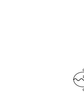
Figure 1: Graphs included in the 2PI effective action $\Gamma_{2}$.

Throughout this paper, we use the Einstein summation convention for repeated indices.

As discussed in detail in Ref. Arts et al. , the second graph in Fig. 1 is proportional to $1/N^{2}$ and is ignored in the 2PI-1/N approximation. Since this term is not present when symmetry is preserved, a comparison of these two approaches requires studying the symmetry breaking case, which is done for the first time here.

III Update equations for the Green functions

We notice from the definitions of the matrices representing $G_{\alpha\beta}(x,x^{\prime})$ and $G_{\alpha\beta}^{-1}(x,x^{\prime})$, that the matrix elements are not inverses of one another, but instead satisfy schematically:

$$D^{-1}D+\bar{K}_{k}^{-1}\bar{K}_{k}=\delta_{\mathcal{C}}\>,$$ (10)

$$D^{-1}K_{j}+\bar{K}_{k}^{-1}G_{kj}=0\>,$$

$$K_{i}^{-1}D+G_{ik}^{-1}\bar{K}_{k}=0\>,$$

$$K_{i}^{-1}K_{j}+G_{ik}^{-1}G_{kj}=\delta_{ij}\delta_{\mathcal{C}}\>.$$

Inverting Eq. (6), we find:

$$D(x,x^{\prime})=\ -g\,\delta_{\mathcal{C}}(x,x^{\prime})$$ (11)

$$+g\int_{\mathcal{C}}\mathrm{d}x_{1}\,\Pi^{\prime}(x,x_{1})\ D(x_{1},x^{\prime})\>,$$

$$G_{ij}(x,x^{\prime})=\ G_{0\,ij}(x,x^{\prime})\delta_{ij}-\int_{\mathcal{C}}\mathrm{d}x_{1}\,G_{0\,ik}(x,x_{1})$$ (12)

$$\times\int_{\mathcal{C}}\mathrm{d}x_{2}\,\Sigma_{kl}^{\prime}(x_{1},x_{2})\,G_{lj}(x_{2},x^{\prime})\>,$$

and

$$K_{i}(x,x^{\prime})=- \int_{\mathcal{C}}\mathrm{d}x_{1}\,\bigl{[}D_{0}^{-1}+\Pi\bigr{]}^{-1}\!(x,x_{1})\,$$ (13)

$$\times\int_{\mathcal{C}}\mathrm{d}x_{2}\,\bigl{[}\bar{K}_{0\,k}^{-1}+\Omega_{k}\bigr{]}(x_{1},x_{2})\,G_{ki}(x_{2},x^{\prime})\>,$$

with the modified polarization

$$\Pi^{\prime}(x,x^{\prime})=\Pi(x,x^{\prime})-\int_{\mathcal{C}}\mathrm{d}x_{1}\,\bigl{[}\bar{K}_{0\,k}^{-1}+\Omega_{k}\bigr{]}(x,x_{1})$$ (14)

$$\times\int_{\mathcal{C}}\mathrm{d}x_{2}\,\bigl{[}G_{0\,kl}^{-1}+\Sigma_{kl}\bigr{]}^{-1}\!(x_{1},x_{2})\,\bigl{[}K_{0\,l}^{-1}+\bar{\Omega}_{l}\bigr{]}(x_{2},x^{\prime})\>,$$

and self-energies

$$\Sigma_{ik}^{\prime}(x,x^{\prime})=\Sigma_{ik}(x,x^{\prime})-\int_{\mathcal{C}}\mathrm{d}x_{1}\,\bigl{[}K_{0\,i}^{-1}+\bar{\Omega}_{i}\bigr{]}(x,x_{1})$$ (15)

$$\times\int_{\mathcal{C}}\mathrm{d}x_{2}\,\bigl{[}D_{0}^{-1}+\Pi\bigr{]}^{-1}\!(x_{1},x_{2})\,\bigl{[}\bar{K}_{0\,k}^{-1}+\Omega_{k}\bigr{]}(x_{2},x^{\prime})\>.$$

These update equations must be solved in conjunction with the one-point functions, Eqs. (5). In the approach of Ref. Arts et al. , the same equations apply with the restriction that $\Omega_{i}=0$ and in the equation for $\Sigma_{ik}^{\prime}$ in Eqs. (9,15), the $\bar{K}_{i}K_{k}$ term is absent.

IV Numerical results and conclusions

We ran simulations for a single component (N=1) $\lambda\,\phi^{4}$ classical field theory, comparing our results to exact Monte Carlo classical calculations, as described in Ref. Mihaila and Dawson (2002). The classical equations become parameter free with a rescaling of variables as discussed in Ref. Aarts et al. (2001). In particular $x,t\rightarrow\mu x,\mu t$ and $\phi\rightarrow\sqrt{3g/\mu^{2}}\phi$. Thus by choosing $g=1/3$, then $\phi$ and time are measured in units of $\mu$ and $1/\mu$. For our initial conditions, we took a thermal gaussian density matrix centered about $\phi(x)=\phi_{0}$ and $\dot{\phi}(x)=\pi_{0}$, thus we are only considering spatially homogeneous evolutions of $\phi$. The details of how to initialize the Green function equations, as well as the solutions for the symmetric case, are discussed in Ref. Blagoev et al. (2001). The numerical procedure for solving the BVA equations is described in Refs. Mihaila and Mihaila (2002); Mihaila and Shaw (2002). Our update procedure conserved energy to better than five significant figures.

The large scale calculations presented in this paper, where the full set of BVA equations is numerically solved, are extremely cost intensive on a computer. Hardware constraints impose an upper limit to the extent to which we can follow the time evolution of the various expectation values. In the following, we choose to describe the time evolution of the system until we observe the thermalization of $\langle\phi^{2}(t)\rangle$ in the case of the exact lattice calculation. Since in the quantum case we expect thermalization to occur faster than in the classical field theory case, we believe that this criteria sets a useful time scale for future calculations in the case of realistic quantum field theory models. In other words, this is the minimum time interval for which we must be able to follow the time evolution, in order to make useful predictions in the quantum case Cooper et al. .

In the symmetric case, the two approximations are very similar and lead to the results shown in Fig. 2. We notice that the time-evolution of the two-point function is well described by the BVA.

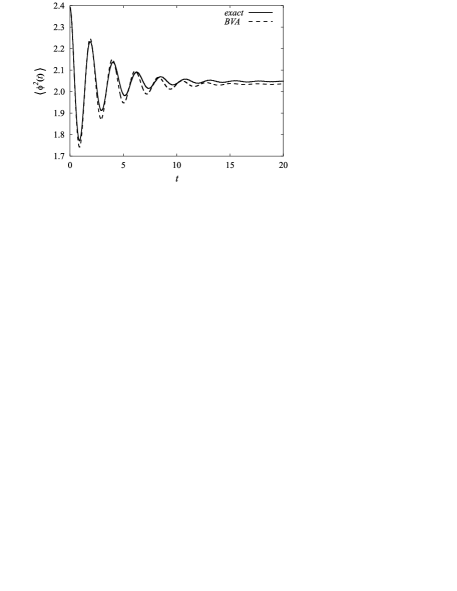
Figure 2: Results for the symmetric case, $\phi(0)=\dot{\phi}(0)=0$.

For the non-symmetric case, we find that the time evolution of the order parameter $\phi(t)$ is better described by the BVA. For the time duration required by the exact calculation for the two-point function to thermalize, the quality of the agreement is similar for all initial values of $\phi(t)$. Typical results are shown in Fig. 3. Here we plot the time evolution of $\langle\phi(t)\rangle$ for a case when the initial symmetry breaking is particularly big. Despite the fact that both the BVA and 2PI-1/N expansion fail to accurately describe $\langle\phi^{2}(t)\rangle$, the BVA reproduces the time evolution of $\langle\phi(t)\rangle$ quite well for almost the entire interval of interest.

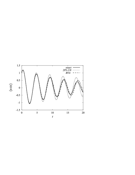
Figure 3: Plot of $\langle\phi(t)\rangle$ for $\phi(0)=1$, and $\dot{\phi}(0)=1$.

For the two-point correlation function the situation is more complicated and depends on the size of the initial symmetry breaking order parameter. The 2PI-1/N expansion thermalizes for all sets of initial conditions we studied, however the time scale for the equilibration process of the two-point function, is not reproduced at large initial symmetry breaking values $\phi(0)\gtrsim 0.4$. The BVA gives an equally good agreement as the 2PI-1/N expansion at small values of $\phi(0)$. However at larger values of $\phi(0)$, the BVA exhibits a non-exponentially decaying oscillatory behavior at intermediate times, before thermalization occurs. This behavior is illustrated in Figs. 4–6, where we gradually increase the initial value of $\phi(0)$. For simplicity, we take $\dot{\phi}(0)=0$ for these cases.

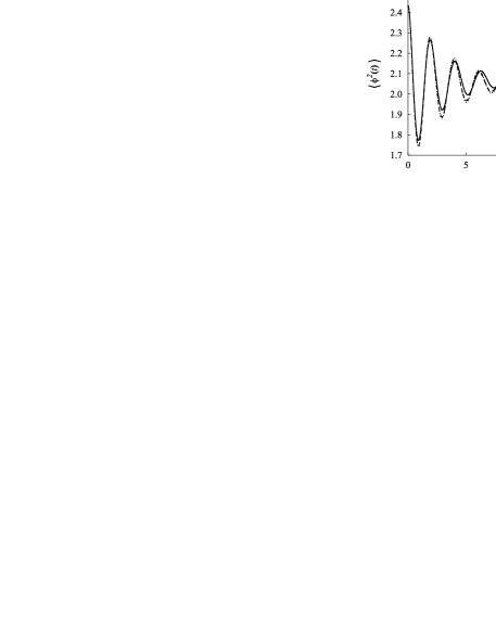
Figure 4: Plot of $\langle\phi^{2}(t)\rangle$ for $\phi(0)=0.2$, and $\dot{\phi}(0)=0$.

Figure 5: Plot of $\langle\phi^{2}(t)\rangle$ for $\phi(0)=0.5$, and $\dot{\phi}(0)=0$.

Figure 6: Plot of $\langle\phi^{2}(t)\rangle$ for $\phi(0)=1$, and $\dot{\phi}(0)=0$.

We see in these figures that the 2PI-1/N result is qualitatively better than the BVA. However, it is important to note that for large values of $\phi(0)$, neither approximation gives the correct damping behavior of the two-point function. This is due to the fact that three-point vertex corrections become important at intermediate time scales. Thus we conclude that although the BVA determines quite well the time evolution of one-point function (the order parameter here), the time evolution of the two-point function requires a better treatment of the three-point vertex.

The accuracy of the BVA depends on the size of the initial symmetry symmetry breaking. This seems to indicate that for a regime where thermalization occurs relatively slowly, such as in the case of this classical field theory model, higher order corrections do eventually become increasingly important at later times. The quantum field theory case is qualitatively different. In the quantum case, thermalization is expected to settle in much faster. Therefore, one can hope that in the quantum case the noise will not have enough time to buildup and consequently will result in a lesser distortion of the BVA predictions. Future studies must go beyond the BVA and investigate the magnitude of these further corrections, especially in the quantum case.

In the above approximations, we set the vertex function to its bare value of unity. However the formalism tells us how to determine the corrections contained in $\Gamma_{2}$. The three-point vertex function is found from the self-energy $\Sigma_{\alpha\beta}$ by:

$$\Gamma_{\alpha\beta\gamma}(x,x^{\prime},x^{\prime\prime})\\ =f_{\alpha\beta\gamma}\,\delta(x,x^{\prime})\,\delta(x,x^{\prime\prime})+\frac{\delta\,\Sigma_{\alpha\beta}(x,x^{\prime})}{\delta\phi_{\gamma}(x^{\prime\prime})}\>,$$ (16)

where $f_{0,i,j}=f_{i,0,j}=f_{i,j,0}=\delta_{ij}$. The integral equation generated from this equation for $\Gamma_{\alpha\beta\gamma}(x,x^{\prime},x^{\prime\prime})$ is discussed in Ref. Mihaila et al. (2001). Thus one way of including vertex corrections is to use the Green functions calculated here to obtain an approximate nonlocal vertex function from Eq. (16), reintroduce the vertex function into the exact SD equation for the two-point function equation and iterate until a stable solution is found. A second approach is to include three loop terms in $\Gamma_{2}$ and solve the resulting set of equations. These approaches will be explored elsewhere.

To conclude, in our quest for an accurate assessment of NLO versus mean-field effects in quantum field theory, the present work represents an important stepping stone. In this paper we report the first results of the full BVA calculation, and in doing so we conclude work done earlier in a more restrictive regime Blagoev et al. (2001). Our goal remains the study of the quantum field theory case, but the classical field theory case is still interesting since this is the high temperature limit of the quantum case. We want to make sure that we know to what extent this limit is reproduced. This is even more important since this is the only case for which exact calculations are possible, and thus the classical field theory O(1) model with one spatial dimension represents a key benchmark.

Having established the domain of applicability of the BVA in this extreme limit, it is clear that two avenues must be explored in the near future: first we will apply the BVA formalism to the study of the quantum linear sigma model, and other realistic models, in 3+1 dimensions, and in doing so we will obtain first insights into the reliability of mean-field approaches in studies of the real-time evolution of realistic quantum field theory models. Next we will investigate the role of further corrections to the BVA, which will be the real test of the accuracy of the BVA formalism. This project will involve the development of practical numerical algorithms and, possibly, require the next generation of supercomputers.