dydiagram

19 July 2002

LAPTH-917/02

hep-ph/0206138

ABSENCE OF SHADOWING IN DRELL-YAN PRODUCTION

AT FINITE TRANSVERSE MOMENTUM EXCHANGE

Stéphane Peigné

LAPTH, BP 110, F-74941 Annecy-le-Vieux Cedex, France

Within a perturbative scalar QED model recently considered by Brodsky et al., we study how leading-twist Coulomb rescatterings affect the Drell-Yan cross section at small $x=x_{target}$, and compare to the case of deep inelastic scattering at small $x_{B}$. We show that in the range where the transverse momentum transferred to the target is large compared to its minimal value $\sim{\cal O}\left(x\right)$, Coulomb rescatterings affect the DIS cross section but not the Drell-Yan production rate. This illustrates that the leading-twist parton distribution functions become non-universal when cross sections which are differential in target-related particles are considered.

1. Introduction and summary

Within the parton model, deep inelastic lepton-nucleon scattering structure functions have been shown to measure the probability to find in the target nucleon a parton with longitudinal momentum fraction $x_{Bjorken}=x_{B}$ in the infinite momentum frame [dy]. This result was obtained in a theory of pions and nucleons for the strong interaction. Since, the correct theory of the strong interaction has been established to be a gauge theory, QCD. According to QCD factorization theorems [fact], at leading-twist the inclusive deep inelastic scattering (DIS) and Drell-Yan (DY) cross sections (in particular) can be factorized and expressed as convolutions between quark and gluon distributions in the incoming hadron(s) and the partonic subprocess cross sections. The predictive power of factorization theorems arises from the statement that parton distribution functions are universal quantities, i.e. independent of the collision. The universality of parton distributions appears to be supported by the data, at least up to some accuracy. Also, the quark distribution (in the nucleon $N$ of momentum $p$) probed in DIS,

$$f_{{\rm q}/N}(x_{B},Q^{2}) = \frac{1}{8\pi}\int dy^{-}\exp(-ix_{B}p^{+}y^{-})$$

$$\times \langle N(p)|{\rm\bar{q}}(y^{-})\gamma^{+}\,{\rm P}\exp\left[ig\int_{0}^{y^{-}}dw^{-}A^{+}(w^{-})\right]{\rm q}(0)|N(p)\rangle$$

where all fields are evaluated at equal light-cone time $y^{+}=0$ and transverse position $\vec{y}_{\perp}=\vec{0}_{\perp}$, seems directly related to the nucleon light-cone wavefunction in $A^{+}=0$ gauge, supporting the probabilistic interpretation of the parton distribution functions (and hence of the DIS structure functions), as in the original parton model.

But the expression (S0.Ex1) is incorrect in $A^{+}=0$ gauge, i.e. the quark distribution is not given by the (squared) nucleon light-cone wavefunction [bhmps]. Roughly speaking, this is because in the Bjorken $\nu\to\infty$ limit, the eikonal coupling of the struck quark of momentum $p_{1}$ to the target color field $A^{\mu}$ satisfies $p_{1}\cdot A\propto\nu A^{+}\to\infty$ in all gauges, except $A^{+}=0$. More precisely, although the light-cone time $y^{+}$ between the absorption and emission of the virtual photon in the forward DIS amplitude vanishes as $1/\nu$, Coulomb interactions occurring in this short time interval actually modify the DIS cross section at leading-twist in all gauges, including the light-cone $A^{+}=0$ gauge [bhmps]. Thus in a gauge theory, the simple identification between parton distribution and parton probability (defined as the square of the nucleon light-cone wavefunction) does not hold. Although not excluded by this observation, the universality of parton distributions becomes much less intuitive. In this respect it was recently shown that single transverse spin asymmetries in semi-inclusive DIS appear at leading-twist [ssabhs], correcting previous statements [0ssacollins]. This is due to the non-universality of spin-dependent parton distributions (in other words of the Sivers asymmetry [sivers]), which originates from the subtle behaviour of Wilson lines under time-reversal [ssacollins]. A possible correct expression in light-cone gauge for the gauge link entering the definition of spin-dependent parton distributions has recently been suggested [jy].

In this context, it is important to reconsider the question of universality of spin-independent parton distributions. In the present work, I compare in a simple model the spin-independent quark distributions probed in DIS and in the Drell-Yan process at small values of $x$. I show that in the range of the exchanged transverse momentum $k_{\perp}$ responsible for leading-twist shadowing in DIS, the Coulomb rescattering corrections a priori modifying the DY cross section are in fact unitary. This is similar to what Bethe and Maximon found in the case of high energy bremsstrahlung and pair production [bm]. Before the advent of QCD, it was also found that corrections to the parton model Drell-Yan formula are actually absent [cw, del]. In the context of gauge theories, our result is an example of the non-universality of the leading-twist parton distributions, which arises when considering a cross section which is differential in the target structure. However, according to the QCD factorization theorem for inclusive cross sections, we expect the $k_{\perp}$-integrated quark distributions probed in DIS and DY to be identical, even though the typical $k_{\perp}$ contributing in both cases is different. We check in Appendix A that this identity indeed occurs within a model where the scale $\sim{\cal O}\left(x\right)$ is screened by a finite photon mass. But the fact that this holds in general, for any target, is not obvious, and we think further studies are needed to settle (or disprove) the universality of parton distributions.

I briefly review in section 2 the model of Brodsky et al. developed in Ref. [bhmps] for DIS shadowing at small $x_{B}$. We recall that this model concentrates on the leading-twist shadowing correction to the DIS cross section (arising from the aligned-jet kinematic region), which can be interpreted as part of the target quark distribution function probed in DIS. The typical value $\langle{k_{\perp}}\rangle_{DIS}$ of the exchanged transverse momentum is found to be of the order of a soft but $x_{B}$-independent scale, $\langle{k_{\perp}}\rangle_{DIS}\sim{\cal O}\left(m\right)$. The model is simply extended to DY production in section 3. Similarly to DIS, the leading-twist Coulomb corrections to the DY cross section arise from a kinematic region which we call the ‘aligned-photon’ region (by analogy with the aligned-jet region of DIS) where the longitudinal momentum fraction taken from the incoming projectile (anti)quark by the radiated virtual photon approaches unity. Those corrections are interpreted as part of the quark distribution probed in the DY process. We find that for $Mx\ll m$, where $M$ is the target mass and $x=x_{target}\ll 1$, the DY cross section is unaffected by Coulomb rescattering at values $k_{\perp}\sim{\cal O}\left(m\right)$, contrary to the DIS cross section. This is the main result of the present paper.

This result is obtained in a scalar QED model and in the limit $x\ll 1$, which allows great technical simplications in the loop calculations. Since we neglect the scale $Mx$ compared to $k_{\perp}$ from the beginning, the $k_{\perp}$-integrated DY cross section is out of reach in the present model. Thus we cannot exclude that the total DY cross section receives a non-zero leading-twist shadowing correction. However, if this happens, the typical value of $k_{\perp}$ responsible for this effect must be, for $x\ll 1$,

$$\langle{k_{\perp}}\rangle_{DY}\sim Mx\ll\langle{k_{\perp}}\rangle_{DIS}$$ (2)

This might have some implications on the properties of momentum broadening and energy loss in the Drell-Yan process. We note that the observed difference between the nuclear broadening of the average transverse momentum in DY production and in dijet photoproduction is not understood [guo]. The result (2) might give some hint to this problem.

But more importantly, it might question the universality of parton distributions at small $x$, as we will discuss in section 4. In this respect, let us note that our result, namely the fact that Coulomb rescatterings do not modify the leading-twist DY Born cross section in the region of transverse momentum exchange $k_{\perp}\gg Mx$, is similar to what was found in Ref. [lrs]. There it was shown, for transverse momenta being large compared to infrared cut-offs (and much smaller than the collision energy), that long-distance contributions to the DY cross section cancel out at the two-loop order. This was argued to be a good indication for the validity of factorization. I stress that it makes on the contrary factorization much less evident, since in the same transverse momentum domain, Coulomb rescatterings modify the DIS cross section, resulting in the observed nuclear shadowing of the DIS parton distributions.

2. Leading-twist shadowing in DIS

2.1 Model for the quark distribution function

A perturbative model for leading-twist DIS shadowing has recently been studied in [bhmps]. Before extending this model to the DY process in the next section, we recall its main features. A specific contribution to $\sigma_{DIS}$ is evaluated, via the optical theorem, from the forward DIS amplitude shown in Fig. 1.

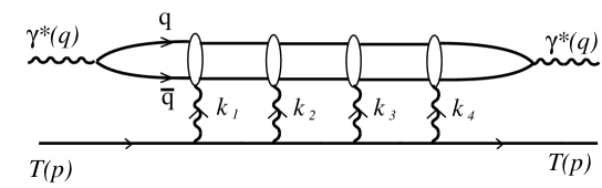
Figure 1: Forward $\gamma^{*}T\to\gamma^{*}T$ amplitude in the DIS model of Ref. [bhmps].

The model is perturbative and chosen to be scalar QED. One takes for the target a scalar “quark” of mass $M$ and momentum $p$, and for the light “quark” and “antiquark” scalars of mass $m$ and momenta $p_{1}$ and $p_{2}$. The couplings of the “gluons” of momenta $k_{i}$ and of the incoming virtual photon of momentum $q$ to the scalars are denoted by $g$ and $e$ respectively. The forward amplitude of Fig. 1 contributes to $\sigma_{DIS}$ through three different cuts between the Coulomb gluon exchanges. Calling $A$, $B$ and $C$ the single, double, and three-gluon exchange amplitudes for the process $\gamma^{*}(q)T(p)\to{\rm q}(p_{1}){\rm\bar{q}}(p_{2})T(p^{\prime})$, the rescattering correction of order $e^{2}g^{8}$ to the Born term $\int|A|^{2}$ reads

$$\Delta\sigma_{DIS}\sim\int\frac{d^{2}\vec{p}_{2\perp}}{(2\pi)^{2}}\,\frac{d^{2}\vec{k}_{\perp}}{(2\pi)^{2}}\,\left[|B|^{2}+2{\rm Re}(A^{*}C)\right]$$ (3)

Feynman diagrams contributing to $A$ are shown in Fig. 2.

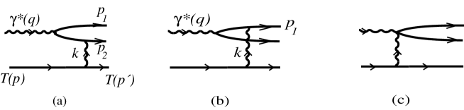
Figure 2: Single gluon exchange DIS amplitude in scalar QED.

The amplitudes $B$ and $C$ are obtained by adding to the Born amplitude $A$ one or two gluon exchanges between the target and the light quarks. In the Bjorken limit and at small $x_{B}$, $\Delta\sigma_{DIS}$ receives a leading-twist contribution, arising from the aligned-jet configuration and presenting the features of a shadowing correction to the DIS Born cross section [bhmps]. It was shown that the kinematic region where leading-twist shadowing appears reads:

$$2\nu\sim p_{1}^{-}\gg p_{2}^{-}\gg k_{\perp},\ k_{i\perp},\ p_{2\perp},\ k_{i}^{-},\ m,\ M\gg k_{i}^{+},\ k^{+},\ p_{2}^{+}\sim{\cal O}\left(Mx_{B}\right)$$ (4)

where when $\nu\to\infty$ the total momentum transfer $k$ satisfies

$$k^{+}=Mx_{B}+p_{2}^{+}$$ (5)

The kinematic limit (4) holds in the target rest frame, where in the four-momentum notation $k=(k^{+},k^{-},\vec{k}_{\perp})$ we have:

$$p = (M,M,\vec{0}_{\perp})$$

$$q = (-Mx_{B},2\nu,\vec{0}_{\perp})$$

$$\epsilon_{L} = \frac{Q}{\nu}(1,-1,\vec{0}_{\perp})$$ (6)

In the case of scalar QED, the leading-twist contribution to $\sigma_{DIS}$ arises from the light quarks coupling to a photon with longitudinal polarization $\epsilon_{L}$.

The scale $\nu$ is the single hard scale in the problem, and the limit $\nu\to\infty$ is taken from the beginning. In the aligned-jet kinematics $q^{-}=2\nu\simeq p_{1}^{-}$, Coulomb rescattering corrections contribute at leading-twist to the DIS cross section [pw]. Compared to the scale $\nu$, the antiquark has a soft momentum $p_{2}$ and must be considered as part of the (soft) target dynamics [fact]. (At small $x_{B}$, $p_{2}^{-}\propto 1/x_{B}$ can however become large enough, so that the physics of destructive interferences between diffractive amplitudes takes place, resulting in shadowing). In addition, the hard vertex $\gamma^{*}{\rm q}\to{\rm q}$ (as viewed in the infinite momentum frame) is taken at zeroth order in the strong coupling $g$. Hence the contribution to $\Delta\sigma_{DIS}$ arising from the domain (4) is a perturbative model for the scaling target quark distribution $f_{{\rm q}/T}(x_{B})$. The leading-twist contribution to $\Delta\sigma_{DIS}$ found in [bhmps] is thus interpreted as shadowing of the quark distribution function in the target.

In order to compare the quark distributions probed in DIS and DY, we will apply the model described above to the DY process in the next section. Let us repeat before the results obtained in [bhmps] for the DIS amplitudes $A$, $B$, $C$ and for the shadowing correction $\Delta\sigma_{DIS}$.

2.2 DIS rescattering amplitudes

Born amplitude

At small $x_{B}$ the Born amplitude for the DIS process is obtained in Feynman gauge from the dominant diagrams of Figs. 2a and 2b, and in light-cone $A^{+}=0$ gauge from the diagram of Fig. 2a only. The gauge invariant result reads in momentum space:

$$A(p_{2}^{-},\vec{p}_{2\perp},\vec{k}_{\perp})=\frac{2eg^{2}MQp_{2}^{-}}{k_{\perp}^{2}}\left[\frac{1}{D(\vec{p}_{2\perp})}-\frac{1}{D(\vec{p}_{2\perp}-\vec{k}_{\perp})}\right]$$ (7)

where

$$D(\vec{p}_{\perp}) = p_{\perp}^{2}+m_{||}^{2}$$ (8)

$$m_{||}^{2} = p_{2}^{-}Mx_{B}+m^{2}$$ (9)

In transverse coordinate space we have

$$\tilde{A}(p_{2}^{-},\vec{r}_{\perp},\vec{R}_{\perp}) = \int\frac{d^{2}\vec{p}_{2\perp}}{(2\pi)^{2}}\,\frac{d^{2}\vec{k}_{\perp}}{(2\pi)^{2}}\,A(p_{2}^{-},\vec{p}_{2\perp},\vec{k}_{\perp})\exp\left(i\vec{r}_{\perp}\cdot\vec{p}_{2\perp}+i\vec{R}_{\perp}\cdot\vec{k}_{\perp}\right)$$ (10)

$$= 2eg^{2}MQp_{2}^{-}\,V(m_{||}r_{\perp})W(\vec{r}_{\perp},\vec{R}_{\perp})$$

The functions $V$ and $W$ stand respectively for the incoming photon wavefunction describing its ${\rm q}{\rm\bar{q}}$ content and for the ${\rm q}{\rm\bar{q}}$ dipole scattering amplitude:

$$V(m\,r_{\perp}) \equiv \int\frac{d^{2}\vec{p}_{\perp}}{(2\pi)^{2}}\frac{e^{i\vec{r}_{\perp}\cdot\vec{p}_{\perp}}}{p_{\perp}^{2}+m^{2}}=\frac{1}{2\pi}K_{0}(m\,r_{\perp})$$ (11)

$$W(\vec{r}_{\perp},\vec{R}_{\perp}) \equiv \int\frac{d^{2}\vec{k}_{\perp}}{(2\pi)^{2}}\frac{1-e^{i\vec{r}_{\perp}\cdot\vec{k}_{\perp}}}{k_{\perp}^{2}}e^{i\vec{R}_{\perp}\cdot\vec{k}_{\perp}}=\frac{1}{2\pi}\log\left(\frac{|\vec{R}_{\perp}+\vec{r}_{\perp}|}{R_{\perp}}\right)$$ (12)

Two-gluon exchange

The gauge invariant expression of the one-loop DIS amplitude $B$ corresponding to two gluon exchanges between the target and the light quarks is [bhmps]:

$$B(p_{2}^{-},\vec{p}_{2\perp},\vec{k}_{\perp})=-ieg^{4}MQp_{2}^{-}\int\frac{d^{2}\vec{k}_{1\perp}}{(2\pi)^{2}}\ \frac{1}{k_{1\perp}^{2}k_{2\perp}^{2}}$$ (13)

$$\times \left[\frac{1}{D(\vec{p}_{2\perp})}-\frac{1}{D(\vec{p}_{2\perp}-\vec{k}_{1\perp})}-\frac{1}{D(\vec{p}_{2\perp}-\vec{k}_{2\perp})}+\frac{1}{D(\vec{p}_{2\perp}-\vec{k}_{\perp})}\right]$$

where $\vec{k}_{2\perp}=\vec{k}_{\perp}-\vec{k}_{1\perp}$. In transverse coordinate space:

$$\tilde{B}(p_{2}^{-},\vec{r}_{\perp},\vec{R}_{\perp})=-ieg^{4}MQp_{2}^{-}V(m_{||}r_{\perp})W^{2}(\vec{r}_{\perp},\vec{R}_{\perp})=\frac{-ig^{2}}{2!}W\tilde{A}$$ (14)

Three-gluon exchange

We give the expression of the three-gluon exchange amplitude $C$ found in [bhmps]:

$$C(p_{2}^{-},\vec{p}_{2\perp},\vec{k}_{\perp})=-\frac{1}{3}eg^{6}MQp_{2}^{-}\int\frac{d^{2}\vec{k}_{1\perp}}{(2\pi)^{2}}\frac{d^{2}\vec{k}_{2\perp}}{(2\pi)^{2}}\ \frac{1}{k_{1\perp}^{2}\,k_{2\perp}^{2}\,k_{3\perp}^{2}}$$

$$\times \left[\frac{1}{D(\vec{p}_{2\perp})}-\frac{3}{D(\vec{p}_{2\perp}-\vec{k}_{1\perp})}+\frac{3}{D(\vec{p}_{2\perp}-\vec{k}_{1\perp}-\vec{k}_{2\perp})}-\frac{1}{D(\vec{p}_{2\perp}-\vec{k}_{\perp})}\right]$$

where $\vec{k}_{3\perp}=\vec{k}_{\perp}-\vec{k}_{1\perp}-\vec{k}_{2\perp}$. In coordinate space:

$$\tilde{C}(p_{2}^{-},\vec{r}_{\perp},\vec{R}_{\perp})=-\frac{1}{3}eg^{6}MQp_{2}^{-}V(m_{||}r_{\perp})W^{3}(\vec{r}_{\perp},\vec{R}_{\perp})=\frac{(-ig^{2})^{2}}{3!}W^{2}\tilde{A}$$ (16)

2.3 The $k_{\perp}$-range in DIS

We stress here that the amplitudes $B$ and $C$ are infrared finite. This is because the quark $p_{1}$ and antiquark $p_{2}$ form a dipole, whose scattering amplitude $W$ vanishes with the separation $r_{\perp}$ between the two quarks (see (12)). Thus in (13) and (S0.Ex7) the typical values of $k_{i\perp}$ are $\sim{\cal O}\left(k_{\perp},p_{2\perp}\right)$. The only other (soft) scale present being $m_{||}$ given in (9), the typical value of the total exchanged transverse momentum $k_{\perp}$ contributing to the $k_{\perp}$-integrated correction $\Delta\sigma_{DIS}$ is:

$$\langle{k_{\perp}}\rangle_{DIS}\sim m_{||}\sim{\cal O}\left(m\right)$$ (17)

The rescattering correction can be obtained from Eqs. (14) and (16):

$$\Delta\sigma_{DIS}\sim\int d^{2}\vec{r}_{\perp}\,d^{2}\vec{R}_{\perp}\,\left[|\tilde{B}|^{2}+2{\tilde{A}}{\tilde{C}}\right]=-\frac{1}{3}\int d^{2}\vec{r}_{\perp}\,d^{2}\vec{R}_{\perp}\,\frac{g^{4}}{4}{\tilde{A}}^{2}W^{2}$$ (18)

This is the leading-twist shadowing correction to the Born DIS cross section found in [bhmps], interpreted as part of the (scalar) quark distribution $f_{{\rm q}/T}(x_{B})$.

3. Rescattering effects in Drell-Yan production

3.1 Model for Drell-Yan production

We now extend the model presented previously for DIS to the Drell-Yan process. This can be done by simply exchanging the virtual photon $q$ and the quark $p_{1}$. We thus describe DY production in the target rest frame where the incoming antiquark has a large ‘minus’ momentum component, $p_{1}^{-}\simeq 2\nu$. As we will see the basic process for DY production in this frame corresponds to quark-antiquark annihilation in the infinite momentum frame.

One diagram contributing to the DY forward amplitude is represented in Fig. 3. All diagrams are simply obtained by taking into account all possible permutations of the lower and upper vertices.

(300,50) v1,v12 v6,v7 fermion,label=$p$,label.side=rightv1,v2 plainv2,i,v3 fermion,label=$p^{\prime}$,label.side=rightv3,v4 plainv4,j,v5 fermion,label=$p$,label.side=rightv5,v6 fermion,label=$p_{1}$,label.side=rightv7,v8 fermionv8,k,v9 fermion,label=$p_{2}$,label.side=rightv9,v10 fermionv10,l,v11 fermion,label=$p_{1}$,label.side=rightv11,v12 photon,label=$k_{1}$,label.side=leftv2,v11 photon,label=$k_{2}$,label.side=leftv3,v10 photon,label=$k_{3}$,label.side=rightv4,v9 photon,label=$k_{4}$,label.side=rightv5,v8 photon,left=.5,label=$q$,label.side=leftl,k

Figure 3: Forward amplitude of order $e^{2}g^{8}$ for the Drell-Yan process. Only one diagram is shown.

The Born DY cross section will get a rescattering correction:

$$\Delta\sigma_{DY}\sim\int\frac{d^{2}\vec{p}_{2\perp}}{(2\pi)^{2}}\,\frac{d^{2}\vec{k}_{\perp}}{(2\pi)^{2}}\,\left[|B_{DY}|^{2}+2{\rm Re}(A_{DY}^{*}C_{DY})\right]$$ (19)

where $A_{DY}$, $B_{DY}$, $C_{DY}$ are the amplitudes for the process ${\rm\bar{q}}(p_{1})T(p)\to\gamma^{*}(q){\rm\bar{q}}(p_{2})T(p^{\prime})$ corresponding to one, two, and three-gluon exchange. In the following we will evaluate these amplitudes in the small $x$ limit.

In the present DY case the photon momentum $q$ is time-like, $q^{2}=Q^{2}>0$ is the final lepton pair invariant mass squared, and the momenta are chosen as ($q^{+}>0$):

$$q = (+Mx,q^{-},\vec{q}_{\perp})$$

$$p_{1} = (p_{1}^{+},2\nu,\vec{0}_{\perp})$$

$$p = (M,M,\vec{0}_{\perp})$$ (20)

where

$$x=\frac{Q^{2}}{2M\nu}$$ (21)

It is easy to check that the configuration $p_{1}^{-}=2\nu\simeq q^{-}\to\infty$, which we call the ‘aligned-photon’ configuration by analogy to the DIS aligned-jet region, gives a leading-twist contribution to $\Delta\sigma_{DY}$. In the DY calculation the same longitudinal photon polarization vector as for DIS can be used.

In the $\nu\to\infty$ limit the total momentum transfer $k$ still satisfies (see (5)):

$$k^{+}=Mx+p_{2}^{+}$$ (22)

The relevant kinematics in the target rest frame is similar to (4),

$$2\nu=p_{1}^{-}\gg p_{2}^{-}\gg k_{\perp},\ k_{i\perp},\ p_{2\perp},\ k_{i}^{-},\ m,\ M,\ q_{\perp}\gg k_{i}^{+},\ k^{+}=Mx+p_{2}^{+}$$ (23)

where one just added the soft $q_{\perp}$ scale.

As in DIS, the antiquark $p_{2}$ is part of the soft target dynamics. The incoming “hadron” is modelled as a single antiquark, whose energy $\nu$ is transferred totally to the virtual photon. Thus in the present model the colliding partons from the projectile and target carry respectively the momentum fractions $x_{1}=1\simeq x_{F}$ and $x_{2}=(k^{+}-p_{2}^{+})/p^{+}=x=Q^{2}/(2M\nu)$. In the infinite momentum frame, we recover quark-antiquark annihilation as the basic partonic process for DY production.

The hard ${\rm q}{\rm\bar{q}}\to\gamma^{*}$ vertex is still taken at zeroth order in $g$, thus all the soft dynamics should be interpreted as part of the target quark distribution, probed at a value $x$ of the longitudinal momentum fraction. Since the shadowing contribution found in DIS describes the target quark distribution probed at $x_{B}=x$, one would naively expect, assuming parton distributions to be universal, to find a rescattering correction to the DY Born cross section originating from the domain (23) equal to that of DIS.

As we will show, in the region (23) the rescattering corrections to $\sigma_{DY}$ are unitary, i.e., do not modify the Born DY cross section, contrary to the DIS case. In this sense the effect of shifting the outgoing quark of DIS to an incoming antiquark in DY is drastic.

3.2 DY rescattering amplitudes

I now give the DY amplitudes in the small $x$ limit. The calculation has been performed both in Feynman and light-cone $A^{+}=0$ gauge, yielding gauge-invariant results. Since different diagrams can contribute in these two gauges, for simplicity the following discussion refers to the Feynman gauge calculation.

Born amplitude

The Born amplitude for the DY process is given in Feynman gauge by the diagrams obtained by exchanging $q$ and $p_{1}$ in Figs. 2a and 2b. The result in the small $x$ limit reads:

$$A_{DY}(p_{2}^{-},\vec{p}_{2\perp},\vec{k}_{\perp})=-\frac{2eg^{2}MQp_{2}^{-}}{k_{\perp}^{2}}\left[\frac{1}{D(\vec{p}_{2\perp})}-\frac{1}{D(\vec{p}_{2\perp}-\vec{k}_{\perp})}\right]$$ (24)

This is equal to the Born amplitude obtained for DIS (see (7)), up to an irrelevant sign. This sign arises since the coupling of the photon brings a factor $\epsilon_{L}\cdot(2p_{1}-q)=Q$ for the DIS amplitude, and $\epsilon_{L}\cdot(q-2p_{1})$ for the DY amplitude. This is due to the fact we consider for DY an incoming antiquark of momentum $p_{1}$.

Two-gluon exchange

In Feynman gauge, the one-loop diagrams which dominate in the small $x$ limit are shown in Fig. 4. The ‘crossed’ diagrams, obtained by permuting the photon coupling vertices to the target line, are also taken into account. We found that the diagrams where the virtual photon emission occurs between the two gluon exchanges are suppressed in this limit (see one example in Fig. 5, where the crossed diagram is also implicitly included). This suppression of radiation in DY production has been mentioned previously [bhq], but we stress here that it occurs only when the transferred momenta $k_{i\perp}$ are large compared to $Mx$, which is precisely the limit studied here (see (23)).

(120,80) v1,v8,p v4,v5,q fermion,label=$p$,label.side=rightv1,i plaini,v2,v3 fermion,label=$p^{\prime}$,label.side=rightv3,v4 fermion,label=$p_{2}$,label.side=rightv5,v6 plainv6,v7,j fermion,label=$p_{1}$,label.side=rightj,v8 photon,tension=0,label=$k_{1}$,label.side=leftv2,v7 photon,tension=0,label=$k_{2}$,label.side=rightv3,v6 photon,label=$q$,label.side=leftj,q                  (120,80) v1,v8,p v4,v5,q fermion,label=$p$,label.side=rightv1,v2 plainv2,v3,i fermion,label=$p^{\prime}$,label.side=righti,v4 fermion,label=$p_{2}$,label.side=rightv5,j plainj,v6,v7 fermion,label=$p_{1}$,label.side=rightv7,v8 photon,tension=0,label=$k_{1}$,label.side=leftv2,v7 photon,tension=0,label=$k_{2}$,label.side=rightv3,v6 photon,label=$q$,label.side=leftj,q

Figure 4: Diagrams contributing dominantly to the two-gluon exchange DY amplitude in Feynman gauge and in the small $x$ limit. Crossed diagrams, obtained by permuting the lower vertices, are included.

(200,80) p,k,p1,i pp,l,p2,q p,v2,u,v1,pp fermion,label=$p$,label.side=rightp,v2 plainv2,u,v1 phantom_arrow,tension=0v2,v1 $p-k_{1}$u phantom_arrowv2,v1 fermion,label=$p^{\prime}$,label.side=rightv1,pp fermion,label=$p_{2}$,label.side=rightp2,v5 fermion,label=$p_{2}-k_{2}$,label.side=leftv5,v4 fermion,label=$p_{1}+k_{1}$,label.side=leftv4,v3 fermion,label=$p_{1}$,label.side=rightv3,p1 photon,tension=0,label=$k_{1}$,label.side=leftv2,v3 photon,tension=0,label=$k_{2}$,label.side=rightv1,v5 photon,label=$q$,label.side=leftv4,q

Figure 5: A diagram (together with the contribution from the crossed one) for the two-gluon exchange DY amplitude which vanishes in the small $x$ limit.