Constraining the absolute neutrino mass scale and Majorana CP violating phases by future $0\nu\beta\beta$ decay experiments

Abstract

Assuming that neutrinos are Majorana particles, in a three generation framework, current and future neutrino oscillation experiments can determine six out of the nine parameters which fully describe the structure of the neutrino mass matrix. We try to clarify the interplay among the remaining parameters, the absolute neutrino mass scale and two CP violating Majorana phases, and how they can be accessed by future neutrinoless double beta ($0\nu\beta\beta$) decay experiments, for the normal as well as for the inverted order of the neutrino mass spectrum. Assuming the oscillation parameters to be in the range presently allowed by atmospheric, solar, reactor and accelerator neutrino experiments, we quantitatively estimate the bounds on $m_{0}$, the lightest neutrino mass, that can be inferred if the next generation $0\nu\beta\beta$ decay experiments can probe the effective Majorana mass ($m_{ee}$) down to $\sim$ 1 meV. In this context we conclude that in the case neutrinos are Majorana particles: (a) if $m_{0}\mathrel{\raise 1.29167pt\hbox{$>$\kern-7.5pt\lower 4.30554pt\hbox{$\sim$}}}300$ meV, i.e., within the range directly attainable by future laboratory experiments as well as astrophysical observations, then $m_{ee}\mathrel{\raise 1.29167pt\hbox{$>$\kern-7.5pt\lower 4.30554pt\hbox{$\sim$}}}30$ meV must be observed; (b) if $m_{0}<300$ meV, results from future $0\nu\beta\beta$ decay experiments combined with stringent bounds on the neutrino oscillation parameters, specially the solar ones, will place much stronger limits on the allowed values of $m_{0}$ than these direct experiments. For instance, if a positive signal is observed around $m_{ee}=10$ meV, we estimate $3\mathrel{\raise 1.29167pt\hbox{$<$\kern-7.5pt\lower 4.30554pt\hbox{$\sim$}}}m_{0}/\text{meV}\mathrel{\raise 1.29167pt\hbox{$<$\kern-7.5pt\lower 4.30554pt\hbox{$\sim$}}}65$ at 95 % C.L.; on the other hand, if no signal is observed down to $m_{ee}=10$ meV, then $m_{0}\mathrel{\raise 1.29167pt\hbox{$<$\kern-7.5pt\lower 4.30554pt\hbox{$\sim$}}}55$ meV at 95 % C.L.

I Introduction

During the last few years, a significant amount of information on the size of the neutrino oscillation parameters have been gathered. Most of what we currently know about these parameters rely on evidences of neutrino flavor transformation that have been collected by the experimental observations of solar solarnu as well as of atmospheric neutrinos atmnu . The evidences coming from solar neutrino data have been strengthened by the recent neutral current measurement at Sudbury Neutrino Observatory (SNO) SNONC whilst those coming from atmospheric neutrinos have also been strongly supported by the K2K accelerator based neutrino oscillation experiment k2k . Furthermore, the negative results of reactor experiments reactors also impose stringent limits on some oscillation parameters.

Assuming that only three active neutrinos participate in oscillations in nature, independent of whether neutrinos are Dirac or Majorana particles, current and future neutrino oscillation experiments can determine at the most six out of the nine parameters which completely describe the neutrino mass matrix, i.e., two mass squared differences ($\Delta m_{12}^{2}$, $\Delta m_{23}^{2}$), three mixing angles ($\theta_{12}$, $\theta_{13}$, $\theta_{23}$) and one CP violating phase ($\delta$) which parametrize the Maki-Nakagawa-Sakata (MNS) MNS leptonic mixing matrix. See, for instance, Refs. oscillation ; kamland for recent discussions on the determination of these oscillation parameters.

However, if neutrinos are of the Majorana type, there remain three non-oscillation parameters, which can not be accessed by oscillation experiments. They are the absolute neutrino mass scale, which can be taken as the lightest neutrino mass, and two extra CP violating Majorana phases Schechter ; Bilenky ; Doi . It is well known that neutrinoless double beta ($0\nu\beta\beta$) decay experiments can shed light on these non-oscillation parameters.

The $0\nu\beta\beta$ decay is a process which can occur if and only if neutrinos are Majorana particles old . A positive signal of $0\nu\beta\beta$ decay always implies a non-zero electron neutrino mass shechter even if it is not induced by the exchange of a light neutrino but by some other mechanism such as the one in supersymmetry models with broken $R$-parity susy . In this work, we assume the simplest possibility to be true, that $0\nu\beta\beta$ decay process is induced only by the exchange of a light neutrino.

It has been abundantly discussed in the literature the relationship between the signals in $0\nu\beta\beta$ decay experiments and oscillation phenomena, see for e.g., Ref. 0nuBB . So far, a large amount of effort has been made to constrain the oscillation parameters from the observation or non-observation of $0\nu\beta\beta$ decay as well as to predict the possible range of the effective Majorana mass in $0\nu\beta\beta$ decay experiments, $m_{ee}$, from the allowed range of oscillation parameters 0nuBB .

In this paper, we take a different point of view. We examine how well we can constrain the three non-oscillation parameters by future $0\nu\beta\beta$ decay experiments, considering that the oscillation parameters will be soon precisely determined (or constrained) by current and future oscillation experiments. We discuss the interplay among these parameters and the observable signal in future $0\nu\beta\beta$ decay experiments for the normal as well as for the inverted ordering of the neutrino mass spectrum. In particular, presuming the oscillation parameters to be in the range presently allowed by the atmospheric, the solar and the reactor neutrino experiments, we examine what can be concluded about these parameters in the case of either a positive or a negative signal is obtained in future $0\nu\beta\beta$ decay experiments 0nuBB-absolute .

So far, no convincing signal of $0\nu\beta\beta$ decay has been observed, rather only an upper bound on $m_{ee}$

$$m_{ee}<350\ \text{meV},$$ (1)

which comes from the result of the Heidelberg-Moscow Collaboration upperbound exists. Recently, an experimental indication of the occurrence of $0\nu\beta\beta$ decay has been announced klapdor01 but since this result seems to be controversial comments , we do not discuss it in this work.

There are many proposals for future $0\nu\beta\beta$ decay experiments to go beyond the bound given in Eq. (1), those include GENIUS GENIUS , CUORE CUORE , EXO EXO , MAJORANA majorana and NOON NOON . It is expected that in the initial phase of the proposed GENIUS experiment GENIUS the sensitivity to $m_{ee}$ can be as low as $\sim$ 10 meV, going down to $\sim$ 2 meV, if the 10 ton version of the experiment is implemented. In this work, we will try to be optimistic and consider that future experiments will eventually inspect $m_{ee}$ down to $\sim$ 1 meV.

The absolute neutrino mass scale is also independently constrained by the tritium decay experiments, which can directly measure the electron neutrino mass, obtaining the upper bound mainz

$$m_{\nu_{e}}<2200\ \text{meV}.$$ (2)

The proposed KATRIN experiment aims to stretch the current sensitivity down to $\sim 340$ meV Katrin . We also take this into consideration in our discussions.

This paper is organized as follows. In Sec. II, we describe the theoretical framework on which we base our work. We first discuss in Sec. III, the dependence of the $0\nu\beta\beta$ signal on the lightest neutrino mass, and second in Sec. IV we discuss how the dependence of $m_{ee}$ on $m_{0}$ is related to the two CP phases, $\alpha_{1}$ and $\alpha_{3}$. In Sec. V we discuss how $m_{ee}^{\text{min}}$, the minimum possible value of $m_{ee}$, depends on $m_{0}$ and $\theta_{13}$. Finally, in Sec. VI, we discuss how the upper as well as the lower bounds on $m_{0}$ depend on the solar neutrino oscillation parameters. Sec. VII is devoted to our discussions and conclusions.

II The Formalism

In this section we discuss the theoretical frame work we will rely upon in this work.

II.1 Mixing and mass scheme

We consider mixing among three neutrino flavors as,

$$\left[\begin{array}[]{c}\nu_{e}\\ \nu_{\mu}\\ \nu_{\tau}\\ \end{array}\right]=U\left[\begin{array}[]{c}\nu_{1}\\ \nu_{2}\\ \nu_{3}\\ \end{array}\right],$$

where $\nu_{\alpha}(\alpha=e,\mu,\tau)$ and $\nu_{i}(i=1,2,3)$ are the weak and the mass eigenstates, respectively, and $U$ is the MNS MNS mixing matrix, which can be parametrized as,

$$\left[\begin{array}[]{ccc}c_{12}c_{13}&s_{12}c_{13}&s_{13}e^{-i\delta}\\ -s_{12}c_{23}-c_{12}s_{23}s_{13}e^{i\delta}&c_{12}c_{23}-s_{12}s_{23}s_{13}e^{i\delta}&s_{23}c_{13}\\ s_{12}s_{23}-c_{12}c_{23}s_{13}e^{i\delta}&-c_{12}s_{23}-s_{12}c_{23}s_{13}e^{i\delta}&c_{23}c_{13}\\ \end{array}\right],$$

where $s_{ij}$ and $c_{ij}$, correspond to sine and cosine of $\theta_{i,j}$. We define the neutrino mass-squared differences as $\Delta m^{2}_{ij}\equiv m^{2}_{j}-m^{2}_{i}$, where $\Delta m^{2}_{\odot}\equiv\Delta m^{2}_{12}$ is relevant for the solutions to the solar neutrino problem, and $\Delta m^{2}_{\text{atm}}\equiv|\Delta m^{2}_{23}|\simeq|\Delta m^{2}_{13}|$ is relevant for the atmospheric neutrino observations.

Current atmospheric neutrino data atmnu indicate that

$$\Delta m^{2}_{\text{atm}}\equiv|\Delta m^{2}_{23}|\simeq(2-4)\times 10^{-3}\ \text{eV}^{2},\ \ \sin^{2}2\theta_{23}\simeq 0.9-1,$$ (3)

which combined with nuclear reactor results reactors imply

$$\sin^{2}\theta_{13}\mathrel{\raise 1.29167pt\hbox{$<$\kern-7.5pt\lower 4.30554pt\hbox{$\sim$}}}0.02,$$ (4)

while the various solar neutrino experiment results strongly suggest that the so called large mixing angle (LMA) MSW solution with parameter in the range solarnu ; SNONC ; sol-recent

$$\Delta m^{2}_{\odot}\equiv\Delta m^{2}_{12}\simeq(2-40)\times 10^{-5}\ \text{eV}^{2},\ \ \tan^{2}\theta_{12}\simeq 0.2-0.8,$$ (5)

will prevail as the explanation to the solar neutrino problem. We will admit throughout this paper that the actual values of these parameters will be confirmed within the above ranges by future neutrino oscillation experiments. Besides further constraining the oscillation parameters given in Eqs. (3)-(5), it is expected that these experiments also can probe the CP violating phase $\delta$ and determine the neutrino mass spectrum (sign of $\Delta m^{2}_{23}$) oscillation .

In this work, we denote the lightest neutrino mass by $m_{0}$. Then using $\Delta m^{2}_{\odot}$ and $\Delta m^{2}_{\text{atm}}$ as defined above, we can describe the two possible mass spectra as follows, (a) Normal mass ordering:

$$m_{1}\equiv m_{0},$$

$$m_{2}\equiv \sqrt{m^{2}_{0}+\Delta m^{2}_{\odot}},$$

$$m_{3}\equiv \sqrt{m^{2}_{0}+\Delta m^{2}_{\odot}+\Delta m^{2}_{\text{atm}}}.$$ (6)

(b) Inverted mass ordering:

$$m_{1}\equiv \sqrt{m^{2}_{0}-\Delta m^{2}_{\odot}+\Delta m^{2}_{\text{atm}}},$$

$$m_{2}\equiv \sqrt{m^{2}_{0}+\Delta m^{2}_{\text{atm}}},$$

$$m_{3}\equiv m_{0}.$$ (7)

In this manner $\Delta m^{2}_{12}=\Delta m^{2}_{\odot}$ for both mass ordering and $\Delta m^{2}_{23}=\pm\Delta m^{2}_{\text{atm}}$ where the $+(-)$ sign indicates normal (inverted) mass ordering. In Fig. 1, a schematic picture of the mass ordering we consider here is shown.

II.2 Effective Majorana mass and $0\nu\beta\beta$

Assuming that the $0\nu\beta\beta$ decay process occurs through the exchange of a light $(m_{\nu}<10$ MeV) neutrino, the theoretically expected half-life of the $0\nu\beta\beta$ decay, $T^{0\nu}_{1/2}$, is given by vogel ,

$$[T^{0\nu}_{1/2}]^{-1}=G^{0\nu}|M_{0\nu}|^{2}m_{ee}^{2},$$ (8)

where $G^{0\nu}$ denotes the exact calculable phase space integral, $M_{0\nu}$ consist of the sum of the Gamow-Teller and the Fermi nuclear matrix elements defined as in Ref. vogel and $m_{ee}$ is the effective Majorana mass defined in Eq. (9) below.

It is known that the evaluation of the nuclear matrix elements suffers from a large uncertainty depending on the adopted method used in the calculations. As we can see in Table II of Ref. vogel , the evaluated half-lives for a given nucleus and a given value of $m_{ee}$ typically vary within a factor of $\sim$ 10 comparing the largest and smallest predicted values. This implies a factor of $\sim$ 3 difference between the minimum and the maximum values of $m_{ee}$ when extracting it from the results of $0\nu\beta\beta$ decay experiments, which in fact directly measure or constrain not $m_{ee}$ but the value of $T^{0\nu}_{1/2}$. This is clear from Eq. (8). In Sec. VI, we will consider for our estimations a somewhat optimistic uncertainty of a factor $\sim$ 2 instead of 3, assuming future improvements on the evaluation of the nuclear matrix elements.

The effective Majorana mass, $m_{ee}$, is given by,

$$m_{ee} = |m_{1}U^{2}_{e1}+m_{2}U^{2}_{e2}+m_{3}U^{2}_{e3}|,$$ (9)

$$= |m_{1}c^{2}_{12}c^{2}_{13}e^{2i\alpha_{1}}+m_{2}s^{2}_{12}c^{2}_{13}+m_{3}s^{2}_{13}e^{2i\alpha_{3}}|,$$

where we have chosen to attach the CP violating phases to the first and third elements. Note that $\alpha_{1}$ and $\alpha_{3}$ must be understood as the relative phases of $U_{e1}$ and $U_{e3}$ with respect to that of $U_{e2}$. The range of these phases are

$$0\leq\alpha_{1}\leq\pi,\ \ 0\leq\alpha_{3}\leq\pi.$$ (10)

As it is known, the value of $m_{ee}$ can be perceived as the norm of the sum of three vectors $\vec{m}_{ee}^{(1)}$, $\vec{m}_{ee}^{(2)}$ and $\vec{m}_{ee}^{(3)}$ in the complex plane whose absolute values are given by,

$$m_{ee}^{(1)} \equiv |\vec{m}_{ee}^{(1)}|\equiv|U^{2}_{e1}|m_{1}=m_{1}c^{2}_{12}c^{2}_{13},$$

$$m_{ee}^{(2)} \equiv |\vec{m}_{ee}^{(2)}|\equiv|U^{2}_{e2}|m_{2}=m_{2}s^{2}_{12}c^{2}_{13},$$

$$m_{ee}^{(3)} \equiv |\vec{m}_{ee}^{(3)}|\equiv|U^{2}_{e3}|m_{3}=m_{3}s^{2}_{13}.$$ (11)

Explicitly, $m_{ee}$ is expressed as

$$m_{ee}^{2} = [m_{ee}^{(1)}\cos 2\alpha_{1}+m_{ee}^{(2)}+m_{ee}^{(3)}\cos 2\alpha_{3}]^{2}+[m_{ee}^{(1)}\sin 2\alpha_{1}+m_{ee}^{(3)}\sin 2\alpha_{3}]^{2},$$ (12)

$$= [m_{ee}^{(1)}]^{2}+[m_{ee}^{(2)}]^{2}+[m_{ee}^{(3)}]^{2}+2\left\{\right.m_{ee}^{(1)}m_{ee}^{(2)}\cos 2\alpha_{1}$$

$$+m_{ee}^{(2)}m_{ee}^{(3)}\cos 2\alpha_{3}+m_{ee}^{(1)}m_{ee}^{(3)}\cos[2(\alpha_{1}-\alpha_{3})]\left.\right\},$$

$$= m_{1}^{2}c^{4}_{12}c^{4}_{13}+m_{2}^{2}s^{4}_{12}c^{4}_{13}+m_{3}^{2}s^{4}_{13}+2\left\{\right.m_{1}m_{2}c^{2}_{12}s^{2}_{12}c^{2}_{13}\cos 2\alpha_{1}$$

$$+m_{2}m_{3}s^{2}_{12}c^{2}_{13}s^{2}_{13}\cos 2\alpha_{3}+m_{1}m_{3}c^{2}_{12}c^{2}_{13}s^{2}_{13}\cos[2(\alpha_{1}-\alpha_{3})]\left.\right\}.$$

We can clearly see from Eq. (12) that $m_{ee}$ is invariant under the transformation

$$(\alpha_{1},\alpha_{3})\rightarrow(\pi-\alpha_{1},\pi-\alpha_{3}),$$ (13)

which allows us to further restrict the range of $(\alpha_{1},\alpha_{3})$, without loss of generality, to

$$0\leq\alpha_{1}\leq\pi,\ \ 0\leq\alpha_{3}\leq\pi/2.\ \$$ (14)

We note that $\alpha_{1}$ and/or $\alpha_{3}$ different from 0 and $\pi/2$ imply CP violation.

The maximum possible value of $m_{ee}$, denoted by $m_{ee}^{\text{max}}$, is given by,

$$m_{ee}^{\text{max}} = m_{ee}^{(1)}+m_{ee}^{(2)}+m_{ee}^{(3)},$$ (15)

$$= (m_{1}c^{2}_{12}+m_{2}s^{2}_{12})c^{2}_{13}+m_{3}s^{2}_{13}.$$

which occurs for $\alpha_{1}=\alpha_{3}=0$. On the other hand, the minimum possible value of $m_{ee}$ is zero only when the three vectors $\vec{m}_{ee}^{(i)}\ (i=1,2,3)$ can form a triangle. This can occur when the condition,

$$m_{ee}^{(i)}<\sum_{j\neq i}m_{ee}^{(j)}\ \ \ (i=1,2,3),$$ (16)

is satisfied. When these three vectors can not form a closed triangle, which includes the case when one of them is null, the minimum value is given by twice the length of the largest vector minus the sum of the norm of all three vectors,

$$m_{ee}^{\text{min}}=2\max\{m_{ee}^{(1)},m_{ee}^{(2)},m_{ee}^{(3)}\}-[m_{ee}^{(1)}+m_{ee}^{(2)}+m_{ee}^{(3)}].$$ (17)

The values of ($\alpha_{1}$, $\alpha_{3}$) which lead to such a minimum are ($\alpha_{1}$, $\alpha_{3}$) = ($\pi/2$, 0), ($\pi/2$, $\pi/2$) or ($0$, $\pi/2$) when respectively $m_{ee}^{(1)}$, $m_{ee}^{(2)}$ or $m_{ee}^{(3)}$ is the largest contribution.

II.3 Some useful extreme limits

To help the comprehension of our discussions in the following sections, let us review here the approximated expressions for $m_{ee}^{\text{max}}$ and $m_{ee}^{\text{min}}$ for the two extreme cases of the absolute neutrino mass scale: vanishing $m_{0}$ and very large $m_{0}$ compared to $\sqrt{\Delta m^{2}_{\text{atm}}}$. The neutrino oscillation parameters are assumed to lie in the ranges given in Eqs. (3)-(5).

(i) Vanishing $m_{0}$ limit:

For the normal mass ordering we have,

$$m_{ee}^{\text{min}},m_{ee}^{\text{max}}\simeq m_{ee}^{(2)}\mp m_{ee}^{(3)}\simeq\sqrt{\Delta m^{2}_{\odot}}s^{2}_{12}c^{2}_{13}\mp\sqrt{\Delta m^{2}_{\text{atm}}}s^{2}_{13},$$ (18)

where the $-(+)$ sign corresponds to $m_{ee}^{\text{min}}$ $(m_{ee}^{\text{max}})$.

For the inverted mass ordering we have,

$$m_{ee}^{\text{min}} \simeq m_{ee}^{(1)}-m_{ee}^{(2)}\simeq\sqrt{\Delta m^{2}_{\text{atm}}}\cos 2\theta_{12}c^{2}_{13},$$ (19)

$$m_{ee}^{\text{max}} \simeq m_{ee}^{(1)}+m_{ee}^{(2)}\simeq\sqrt{\Delta m^{2}_{\text{atm}}}c^{2}_{13}.$$ (20)

(ii) Large $m_{0}$ ($\gg\sqrt{\Delta m^{2}_{\text{atm}}}$) limit:

For the normal as well as for the inverted mass ordering,

$$m_{ee}^{\text{min}} \simeq m_{ee}^{(1)}-m_{ee}^{(2)}-m_{ee}^{(3)}\simeq m_{0}(c^{2}_{13}\cos 2\theta_{12}-s^{2}_{13}),$$ (21)

$$m_{ee}^{\text{max}} \simeq m_{ee}^{(1)}+m_{ee}^{(2)}+m_{ee}^{(3)}\simeq m_{0}.$$ (22)

III Dependence on the lightest neutrino mass

In this section we examine how the effective Majorana mass, $m_{ee}$, depends on the lightest neutrino mass, $m_{0}$, and clarify the importance of each of the individual contributions, $m_{ee}^{(1)}$, $m_{ee}^{(2)}$ and $m_{ee}^{(3)}$ to $m_{ee}$. We present in Fig. 2 for normal (upper panels) as well as inverted (lower panels) mass ordering, the maximum and minimum values of $m_{ee}$ as a function of $m_{0}$ for vanishing $\theta_{13}$ (left panels) and $\sin^{2}\theta_{13}=0.02$ (right panels). In the same plots we also show the individual contributions of $m_{ee}^{(1)}$, $m_{ee}^{(2)}$ and $m_{ee}^{(3)}$ by dashed, dotted and dash-dotted lines, respectively.

Let us first discuss the case of normal mass ordering. As we can see from the plots in the upper panels of Fig. 2, for smaller values of $m_{0}$, $m_{ee}^{(2)}$ is the dominant contribution whereas for larger values of $m_{0}$, $m_{ee}^{(1)}$ dominates over the other contributions. For the typical values of the oscillation parameters allowed by the solar, atmospheric neutrino and reactor data, $m_{ee}^{(3)}$ is almost always the smallest contribution to $m_{ee}$, being subdominant in $m_{ee}$ and it can only be important when there is a large cancelation between $m_{ee}^{(1)}$ and $m_{ee}^{(2)}$.

It is clear that a strong cancelation in $m_{ee}$ can occur if at least two of $m_{ee}^{(1)}$, $m_{ee}^{(2)}$ and $m_{ee}^{(3)}$ are comparable in magnitude. Just by comparing their magnitudes in the plots in Fig. 2, we can easily see for which values of $m_{0}$ a strong cancelation in $m_{ee}$ can occur. For the case if $\theta_{13}=0$, $m_{ee}$ can be zero only at one particular value of $m_{0}$ (see Fig. 2 (a)) whereas for the case if $\theta_{13}\neq 0$ $m_{ee}$ can be zero for some range of $m_{0}$ (see Fig. 2(b)). See Sec. V for more detailed discussions about the dependence of $m_{ee}^{\text{min}}$ on $m_{0}$ and $\theta_{13}$.

In the case of inverted mass ordering, the situation changes significantly. Here $m_{ee}^{(1)}>m_{ee}^{(2)}>>m_{ee}^{(3)}$ and $m_{ee}^{\text{min}}\neq 0$ always must satisfy the condition,

$$m_{ee}^{\text{min}}\mathrel{\raise 1.29167pt\hbox{$>$\kern-7.5pt\lower 4.30554pt\hbox{$\sim$}}}\sqrt{\Delta m^{2}_{\text{atm}}}\cos 2\theta_{12}\sim 10\ \ \text{meV},$$ (23)

for any value of $m_{0}$ for current allowed parameters from solar and atmospheric neutrino data and no complete cancelation in $m_{ee}$ is expected as we can see clearly from the plots in the lower panels of Fig. 2. Therefore, if no positive signal of $0\nu\beta\beta$ is observed down to $\sim 10$ meV, inverted mass ordering can be excluded as long as neutrinos are Majorana particles.

IV Dependence on the lightest neutrino mass and CP phases

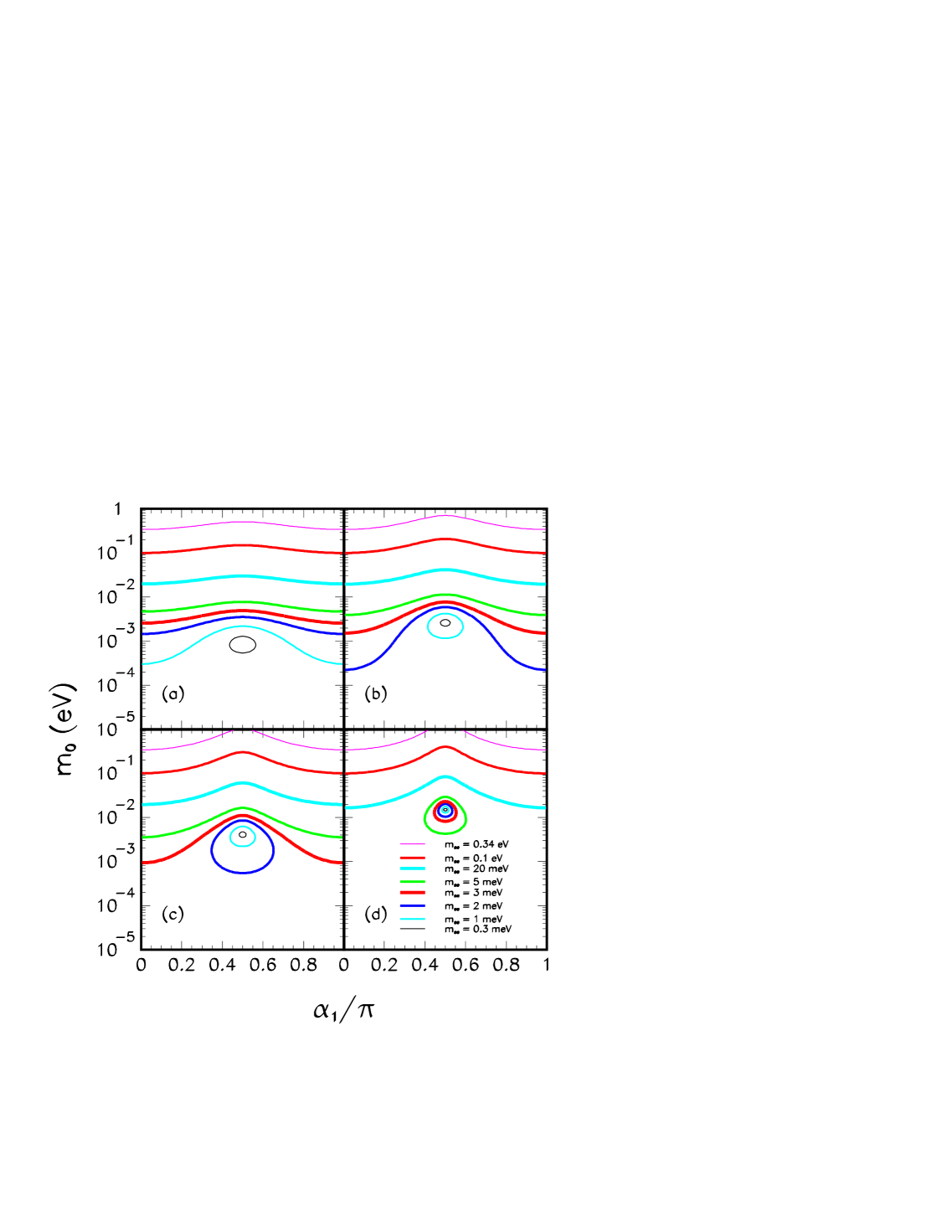
Figure 3: Iso-contour plots of $m_{ee}$ for $\sin^{2}\theta_{13}=0$ for the normal mass ordering in the $\alpha_{1}-m_{0}$ plane. We have fixed the other relevant mixing parameters as ($\Delta m^{2}_{12}$, $\tan^{2}\theta_{12}$) = (2$\times 10^{-5}$ eV², 0.2) in (a), (5$\times 10^{-5}$ eV², 0.35) in (b), (5$\times 10^{-5}$ eV², 0.5) in (c) and (4$\times 10^{-4}$ eV², 0.6) in (d).

Let us next discuss how the $m_{ee}$ dependence on $m_{0}$ is related to the two CP phases, $\alpha_{1}$ and $\alpha_{3}$. We present in Fig. 3 iso-contour plots of $m_{ee}$ in the $m_{0}$-$\alpha_{1}$ plane for vanishing $\theta_{13}$, for the normal mass ordering, for some values of the solar parameters taken within the allowed ranges given in Eq. (5). Note that, in this particular case, there is no dependence on the phase $\alpha_{3}$ in our choice of parametrization, which is clear from Eq. (9).

Fist we note that in the plots, iso-contours are symmetric with respect to $\alpha_{1}/\pi=0.5$. Second we note that if $m_{ee}$ is smaller than certain value, $m_{ee}^{\text{crit}}$, the iso-contours are closed which means that the possible values of both $m_{0}$ and $\alpha_{1}$ are bounded to some limited range, which does not include zero. The critical value of $m_{ee}$ under which the contour is a closed one is given by

$$m_{ee}^{\text{crit}}\simeq m_{ee}^{(2)}=\sqrt{\Delta m^{2}_{\odot}}s^{2}_{12}\simeq(1-10)\ \text{meV},$$ (24)

this dependence is illustrated in Fig. 3. If a positive $0\nu\beta\beta$ signal is not observed down to these values, this will imply either that $m_{0}$ as well as the CP phase $\alpha_{1}$ are bounded to the limited range within the closed contours shown in Fig. 3 or that neutrinos are of not Majorana type particles.

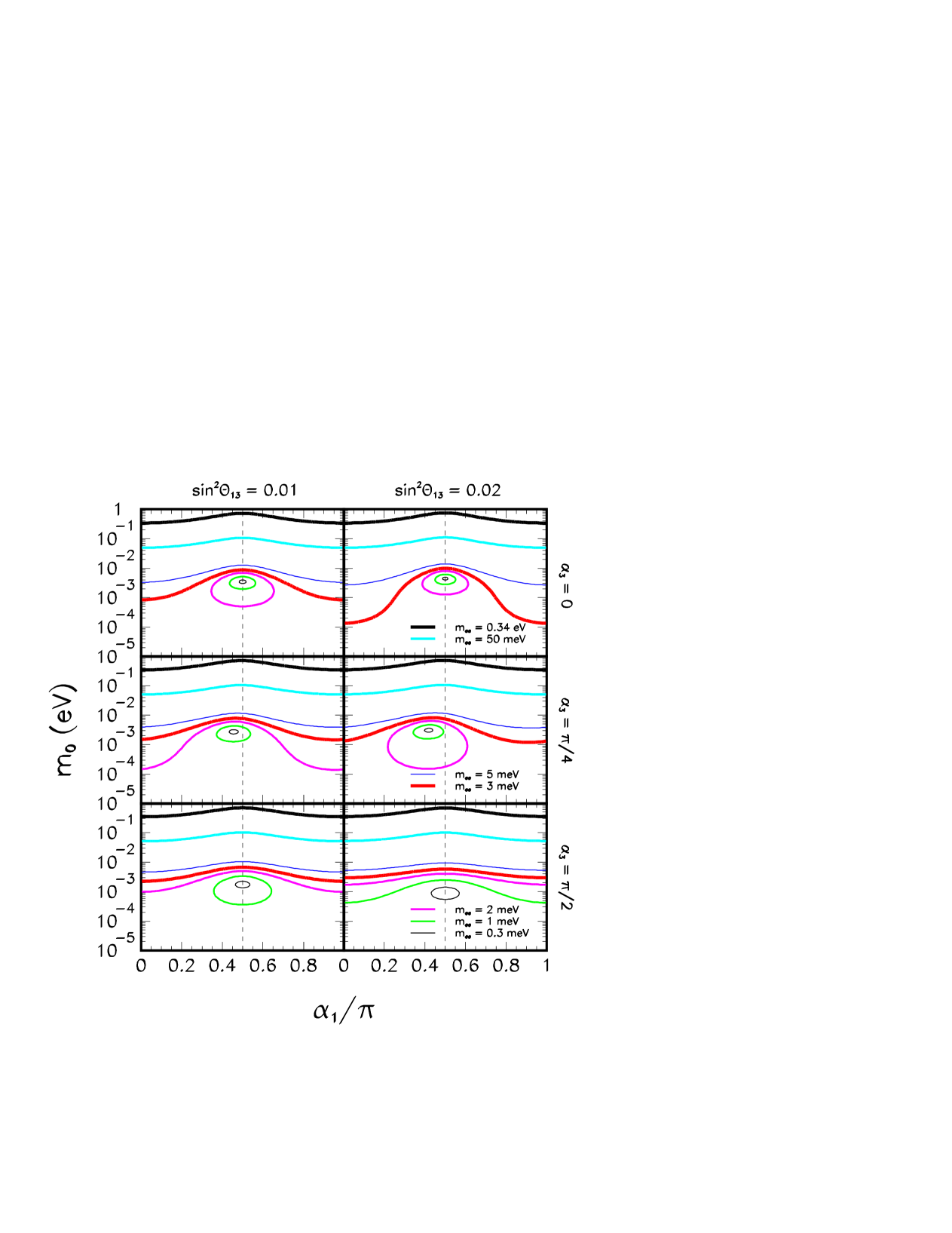
Figure 4: Same as Fig. 3(b) but for $\sin^{2}\theta_{13}=0.01$ (left panels) and 0.02 (right panels), for $\alpha_{3}=0$ (upper panels), $\pi/4$ (middle panels) and $\pi/2$ (lower panels). The dashed vertical lines mark $\alpha_{1}/\pi=0.5$.

We show in Fig. 4 the same information as in Fig. 3(b) but for $\sin^{2}\theta_{13}=0.01$ (left panels) and 0.02 (right panels) for three different values of $\alpha_{3}=0,\pi/4$ and $\pi/2$ in the upper, middle and lower panels, respectively. As we can see from these plots the qualitative behaviors of the contours are very similar to those in Fig. 3(b). This is due to the fact that $m_{ee}^{(3)}$, which is the only term that carries the contributions of $\sin^{2}\theta_{13}$ and $\alpha_{3}$, is subdominant compared to the other two elements in $m_{ee}$. The effect of a non-zero $\alpha_{3}$ is to cause some displacement of the position of the symmetry line of the plots from around $\alpha_{1}/\pi=0.5$ to somewhat smaller values.

Let us here mention the case where $m_{0}$ can be independently measured by another experiment such as the KATRIN Katrin tritium decay one. In this case, it is possible to constrain the CP phase $\alpha_{1}$ by comparing the measured values of $m_{ee}$ and $m_{0}$ provided that $m_{0}\mathrel{\raise 1.29167pt\hbox{$>$\kern-7.5pt\lower 4.30554pt\hbox{$\sim$}}}340$ meV, the maximum sensitivity of KATRIN. If a $0\nu\beta\beta$ decay experiment measures $m_{ee}$ significantly smaller than $m_{0}$ measured by KATRIN, this would imply a non-zero CP phase $\alpha_{1}$. This is because for the $m_{0}$ values relevant for KATRIN, $m_{ee}\sim m_{0}$ if $\alpha_{1}\simeq 0$, but $m_{ee}$ can be as small as $\sim 0.1\times m_{0}$ if $\alpha_{1}\sim\pi/2$ and if the largest allowed value of $\theta_{12}$ from the current LMA allowed region is realized (see Eqs. (21) and (22)). However, it would still be difficult to say something definite about the value of $\alpha_{1}$ for 10 $\mathrel{\raise 1.29167pt\hbox{$<$\kern-7.5pt\lower 4.30554pt\hbox{$\sim$}}}m_{0}/\text{meV}\mathrel{\raise 1.29167pt\hbox{$<$\kern-7.5pt\lower 4.30554pt\hbox{$\sim$}}}$ 340.

Our plots in Figs. 3 and 4 are in agreement with the conclusion presented in Ref. barger , that is, either a positive or a negative results in a $0\nu\beta\beta$ decay experiment can constrain $m_{0}$ and $\alpha_{1}$ but, since the possible values of $\alpha_{1}$ will always include $\pi/2$, a non-zero value of $\alpha_{1}$ cannot be interpreted as an evidence of CP violation, even if a positive signal of $0\nu\beta\beta$ decay is observed. Unfortunately, to be able to say anything more definite on the CP phase, independent precise information on $m_{0}$ is unavoidable. Moreover, nothing can be concluded about the value of $\alpha_{3}$.

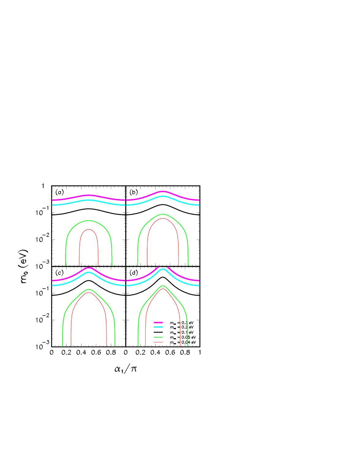
Figure 5: Same as Fig. 3 but for the inverted mass ordering. Here we have fixed the atmospheric mass scale to $\Delta m^{2}_{23}=-5\times 10^{-3}$ eV² in (a), to $\Delta m^{2}_{23}=-3\times 10^{-3}$ eV² in (b) and (c) and to $\Delta m^{2}_{23}=-1.3\times 10^{-3}$ eV² in (d).

We show in Fig. 5 the same information as in Fig. 3 for the inverted mass ordering. Since there is no significant dependence on $\theta_{13}$ or on $\alpha_{3}$ in this case, we show only the curves for vanishing $\theta_{13}$. We note from these plots that there is no lower bound for $m_{0}$ as long as $m_{ee}\mathrel{\raise 1.29167pt\hbox{$<$\kern-7.5pt\lower 4.30554pt\hbox{$\sim$}}}50$ meV, and moreover, $\alpha_{1}$ is less constrained if compared to the case of normal ordering, independently of the values of the other neutrino oscillation parameters.

For the case of the normal mass ordering, we have also investigated if the uncertainties in the determination of the solar parameters as well as on $m_{ee}$ can wash out the determination of a non-zero CP phase $\alpha_{1}$, expected by the closed contours in Figs. 3 and 4. For four different central values of $m_{ee}$, assuming 30% uncertainty in their determination (see Sec. VI for a detailed explanation), we have obtained the region in the ($\Delta m^{2}_{12}$, $\tan^{2}\theta_{12}$) plane where $\alpha_{1}$ can be constrained to a non-zero value for (i) $\sin^{2}\theta_{13}=0$ and (ii) $\sin^{2}\theta_{13}=0.02$. This is shown in Fig. 6, where we also have assumed for each point in the ($\Delta m^{2}_{12}$, $\tan^{2}\theta_{12}$) plane a 10 % uncertainty in the determination of these two parameters. In this plot we have indicated by crosses the set of solar parameters used in Fig. 3(a)-(d).

We observe that for the case of $\theta_{13}=0$ (see Fig. 6 (i)), determination of a non-zero CP phase $\alpha_{1}$ is possible as long as one can reach the sensitivity $m_{ee}\mathrel{\raise 1.29167pt\hbox{$<$\kern-7.5pt\lower 4.30554pt\hbox{$\sim$}}}5$ meV for the paramerter set (d) and $m_{ee}\mathrel{\raise 1.29167pt\hbox{$<$\kern-7.5pt\lower 4.30554pt\hbox{$\sim$}}}1$ meV for sets (b) and (c). On the other hand, in the case where $\sin^{2}\theta_{13}=0.02$, as we can see from Fig. 6 (ii), a better sensitivity in $m_{ee}$ is required to establish non-zero $\alpha_{1}$ value for the same parameter set. This is because when $\theta_{13}$ is non-zero, third element $m_{ee}^{(3)}$, which contains another CP phase, $\alpha_{3}$, whose value is assumed to be unknown, comes into play and this could wash out more efficiently the determination of non-zero $\alpha_{1}$ when compared to the case where $\theta_{13}=0$.

V Dependence on the lightest neutrino mass and $\theta_{13}$

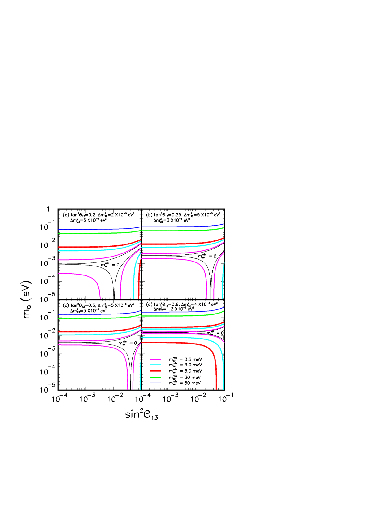
Figure 7: Iso-contour plots of $m_{ee}^{\text{min}}$ in the $s_{13}^{2}-m_{0}$ plane for different choices of the mixing parameters for the normal mass ordering. We note that in the region delimited by thin solid curves $m_{ee}^{\text{min}}=0$.

In this and the next sections we focus on the relation among $m_{ee}$ and some of the yet undetermined mixing parameters. Let us start by discussing the dependence of $m_{ee}^{\text{min}}$ on $m_{0}$ and $\theta_{13}$. Here we discuss only the case of normal ordering since the dependence on $\theta_{13}$ for the inverted case is quite small. We present in Fig. 7, the iso-contour plots of $m_{ee}^{\text{min}}$ in the $s^{2}_{13}$-$m_{0}$ plane for some different choices of the oscillation parameters.

For vanishing $\theta_{13}$, one can have $m_{ee}^{\text{min}}=0$ if $m_{ee}^{(1)}=m_{ee}^{(2)}$, i.e. , $m_{1}c^{2}_{12}=m_{2}s^{2}_{12}$, which is equivalent to,

$$m_{0}=\frac{s^{2}_{12}}{\sqrt{|\cos 2\theta_{12}|}}\sqrt{\Delta m^{2}_{\odot}}\sim 3\ \text{meV},$$ (25)

where we have computed the numerical estimate using the best fitted values of the parameters from the latest solar neutrino data (see Fig. 2(a) and Fig. 7(b)). Within the current allowed range given in Eq. (5), the possible values of $m_{0}$ for which we can expect strong cancelation are in the range $m_{0}\simeq(0.9-12)\ \text{meV}$, as we can confirm with the plots in Fig. 7.

For non-zero values of $\theta_{13}$, as we can see clearly from Fig. 7, $m_{ee}^{\text{min}}$ can take zero for some range of $m_{0}$. We can also see that there is a critical value of $\theta_{13}$ for which $m_{ee}^{\text{min}}$ is zero with vanishing $m_{0}$. Such a value of $\theta_{13}$ can be easily estimated by solving $m_{2}c^{2}_{13}s^{2}_{12}=m_{3}s^{2}_{13}$ with $m_{0}\rightarrow 0$ which is equivalent to,

$$s^{2}_{13}\simeq\sqrt{\frac{\Delta m^{2}_{\odot}}{\Delta m^{2}_{\text{atm}}}}s^{2}_{12}\sim 0.03,$$ (26)

for the best fitted parameters from solar as well as atmospheric neutrino data. We note that this is close to the current upper bound on $s^{2}_{13}$ allowed by the CHOOZ result reactors . Letting $\Delta m^{2}_{\odot}$, $\Delta m^{2}_{\text{atm}}$ and $s^{2}_{12}$ take any value in the region consistent with the solar and atmospheric neutrino observations given in Eq. (3) and (5), the range of $s^{2}_{13}$ for which strong cancelation can occur is $s^{2}_{13}\simeq 0.01-0.20$, which is again consistent with our results in Fig. 7.

We observe that if $s^{2}_{13}$ is smaller than the critical value given in Eq. (26), the value of $m_{0}$ can be strongly constrained to some limited range around the value of $m_{0}$ given in Eq. (25), provided that future $0\nu\beta\beta$ experiment can probe a $m_{ee}$ value as small as $\sim\sqrt{\Delta m^{2}_{\odot}}s^{2}_{12}$ independent of whether a positive or negative signal of $0\nu\beta\beta$ is observed.

VI Constraining $m_{0}$ using solar neutrino data

Finally, let us discuss how we can constrain $m_{0}$ using the solar neutrino parameters. Let us first analyze the case where a positive signal of $0\nu\beta\beta$ is observed. The value of $m_{ee}$ has to be extracted from the experimental measured half-life, $T^{0\nu}_{1/2}$, of the decaying parent nucleus by comparison with the theoretical prediction which rely on nuclear matrix element calculations. This means that the experimental value of $m_{ee}$ has to be expressed as an interval obtained using the maximum and minimum matrix element predictions.

As mentioned in Sec. II.2, typically, there is a factor 3 difference among the results of the matrix element evaluations according to different model assumptions vogel . In order to take such large theoretical uncertainty into account in our estimations, we will first assume that the experimental measured value of $m_{ee}$ will be extracted using the mean between the minimum and maximum values of the matrix element calculations, then attach 30 % uncertainty around this value, which correspond to a factor $\sim$ 2 between the smallest and the largest theoretically allowed $m_{ee}$ values for a given value of the observed half-life. This is a somewhat optimistic but reasonable assumption. Hopefully improvements on the understanding of the underlining nuclear physics effects can decrease this uncertainty even further.

In Fig. 8 we show the iso-contours of upper ($m_{0}^{\text{max}}$) and lower ($m_{0}^{\text{min}}$) bounds on $m_{0}$ in units of meV in the $\tan^{2}\theta_{12}$-$\Delta m^{2}_{12}$ plane for the case where a positive signal of $0\nu\beta\beta$ is observed with central values $m_{ee}$ = 10, 5, 3 and 1 meV with a 30 % uncertainty. In these plots we have used $\Delta m^{2}_{23}=3\times 10^{-3}$ eV² and $\sin^{2}\theta_{13}=0$. We do not present plots for $m_{ee}>10$ meV, since in these cases the upper and lower bound can be analytically estimated as we will see below.

When $m_{0}>\sqrt{\Delta m^{2}_{\text{atm}}}$ the upper bound on $m_{0}$ does not depend much on $\Delta m^{2}_{\odot}$ but essentially only on $\theta_{12}$ (see Eq. (21) in Sec. II.3), it is given as,

$$m_{0}^{\text{max}}\sim\frac{m_{ee}}{\cos 2\theta_{12}},$$ (27)

and the lower bound $m_{0}^{\text{min}}\sim m_{ee}$, independent of the solar parameters in the region compatible with the LMA MSW solution to the solar neutrino problem.

We observe that, as can be seen in Fig. 8, that as $m_{ee}$ decreases, the upper bound lines, which mainly depend on $\tan^{2}\theta_{12}$, are shifted to larger values of $\theta_{12}$, decreasing $m_{0}^{\text{max}}$ for a given set of $(\tan^{2}\theta_{12},\Delta m^{2}_{12})$. The lower bound lines, on the other hand, depend more on $\Delta m^{2}_{12}$ and there are some regions where no lower bound is obtained. For $m_{ee}\mathrel{\raise 1.29167pt\hbox{$>$\kern-7.5pt\lower 4.30554pt\hbox{$\sim$}}}10$ meV or $m_{ee}\mathrel{\raise 1.29167pt\hbox{$<$\kern-7.5pt\lower 4.30554pt\hbox{$\sim$}}}1$ meV there is always a lower bound found inside the currently allowed LMA MSW region, whereas for $1\mathrel{\raise 1.29167pt\hbox{$<$\kern-7.5pt\lower 4.30554pt\hbox{$\sim$}}}m_{ee}/\text{meV}\mathrel{\raise 1.29167pt\hbox{$<$\kern-7.5pt\lower 4.30554pt\hbox{$\sim$}}}10$ this is not true. The appearance of these no lower bound bands comes from the fact the in these regions the solar mass scale alone is sufficient to explain the positive signal observed, even for vanishing $m_{0}$.

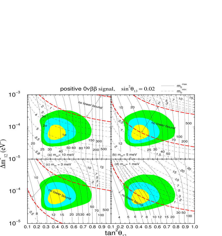
Figure 9: Same as Fig. 8 but for $\sin^{2}\theta_{13}=0.02$.

In Fig. 9 we repeat the same exercise but for $\sin^{2}\theta_{13}=0.02$. The most significant effect of a non zero $\sin^{2}\theta_{13}$ is the increase of the size of the no lower bound band, which can in some cases stretch over the entire LMA allowed region, otherwise the behavior of the upper and lower bound lines is qualitatively similar to the previous case.

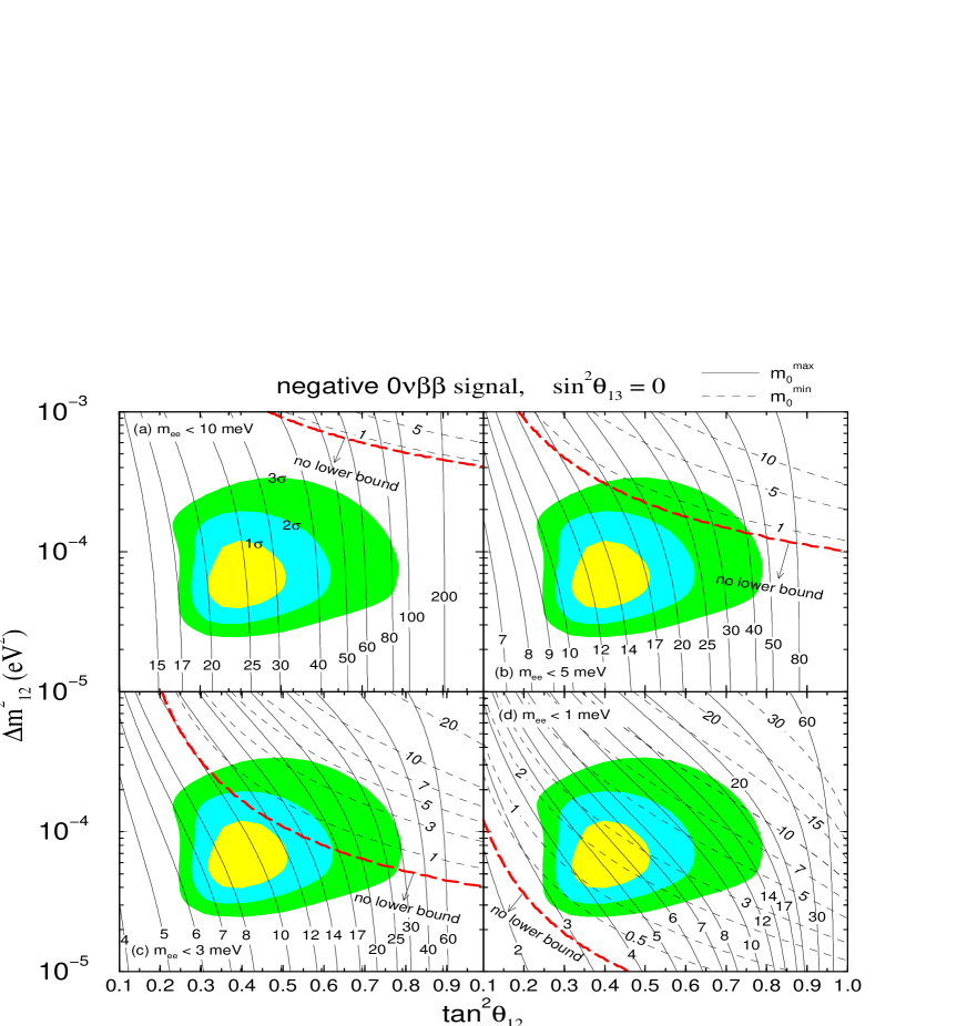
Figure 10: Same as Fig. 8 but for the case where no positive signal of $0\nu\beta\beta$ is observed down to $m_{ee}$ = 10 meV (a), 5 meV (b), 3 meV (c) and 1 meV (d).

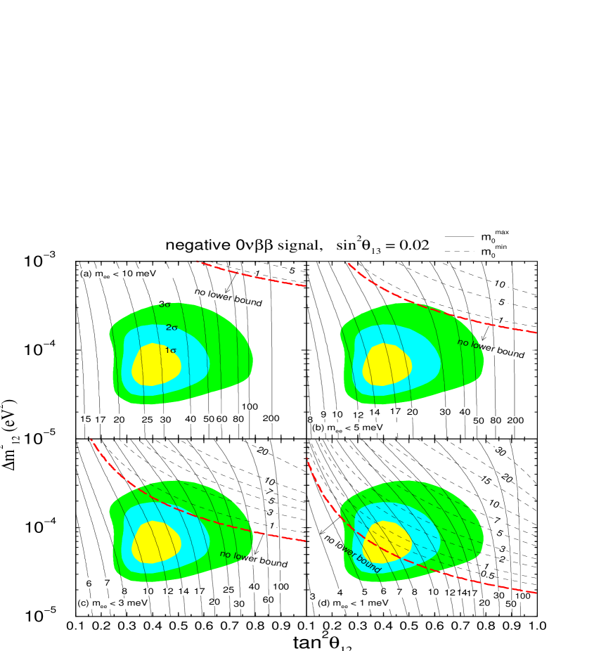
Figure 11: Same as Fig. 10 but for $\sin^{2}\theta_{13}=0.02$.

Let us next consider the case where no positive signal is observed. In Fig. 10 we present the same information as in Fig. 8 but for the case where no positive signal of $0\nu\beta\beta$ is observed down to $m_{ee}$ = 10 meV (a), 5 meV (b), 3 meV (c) and 1 meV (d). It is assumed that when no positive signal is observed, for a given bound on the half-life time, the bounds on $m_{ee}$ are extracted using the smallest nuclear matrix element prediction which lead to the largest $m_{ee}$ value (see Eq. (8)). We can see that qualitative behavior of the iso-contours for the upper bound is similar to that in Fig. 8 but it is different for the trend of the lower bound curves. Compared to the case where positive $0\nu\beta\beta$ signal is obtained, it is more difficult to put lower bound on $m_{0}$. This can be easily understood from Fig. 2 (a). We note that unless we can constrain $m_{ee}$ down to $\sim 3$ meV, no lower bound on $m_{0}$ is obtained. In Fig. 11 we present the same information as in Fig. 10 but for $\sin^{2}\theta_{13}=0.02$. Again, the qualitative behavior of the iso-contours is similar to the case of $\sin^{2}\theta_{13}=0$. The difference from the previous case presented in Fig. 10 is that the constraint on $m_{0}$ become somewhat weaker, leading to larger upper bounds and smaller lower bounds for a given set of $(\tan^{2}\theta_{12},\Delta m^{2}_{12})$.

Finally, let us also comment the case of inverted ordering. For this case, we can easily estimate the upper as well as lower bound from the analytic expressions as well as from the lower panels of Fig. 2. Let us look at Fig. 2 (c) and (d). First of all, if the inverted ordering is the case, the observed value of $m_{ee}$ in $0\nu\beta\beta$ decay experiment must be larger than the value given in Eq. (23), as already mentioned in Sec. III. If the observed $m_{ee}$ is smaller than $\sqrt{\Delta m^{2}_{\text{atm}}}c^{2}_{13}$ (see Eq. (20)) then there is no lower bound on $m_{0}$ whereas the upper bound is given by the same expression for the case of normal ordering, by Eq. (27). If the observed $m_{ee}$ value is larger than $\sqrt{\Delta m^{2}_{\text{atm}}}c^{2}_{13}$, then the upper as well as lower bounds are given by the same expression as in the case of normal ordering, which is already discussed in this section.

VII Discussions and conclusions

We have studied how the non-oscillation neutrino parameters which can not be extracted from the oscillation analysis, the absolute neutrino mass scale and two CP violating Majorana phases, can be accessed by the positive or negative signal of future $0\nu\beta\beta$ decay experiments. We have carried out this by choosing various different set of mixing parameters which are varied within the parameter region currently allowed by the solar, atmospheric as well as by reactor neutrino experiments.

In the future, the KATRIN experiment expects to directly inspect $m_{0}$ down to $\sim$ 340 meV Katrin , while there are several proposed astrophysical measurements on the temperature perturbation in the early universe imprinted in the cosmic microwave background radiation, such as the ones that can be performed by MAP (Microwave Anisotropy Probe) MAP and Planck Planck , which can probe $m_{0}$ down to $\sim$ 300 meV cosmology , where the expected sensitivity suffers from the uncertainty coming from cosmological parameters. It is expected that future supernova neutrino measurements can probe $m_{0}$ down to at most $\sim$ (2-3) eV supernova .

Our analysis permit us to conclude that if these experiments measure $m_{0}\mathrel{\raise 1.29167pt\hbox{$>$\kern-7.5pt\lower 4.30554pt\hbox{$\sim$}}}300$ meV, then either a positive signal of $0\nu\beta\beta$ decay compatible with $m_{ee}\mathrel{\raise 1.29167pt\hbox{$>$\kern-7.5pt\lower 4.30554pt\hbox{$\sim$}}}30$ meV must be observed in the near future or neutrinos are Dirac particles. This is simply because $m_{ee}^{\text{min}}\sim m_{0}\cos 2\theta_{12}$ (see Eq. (21) in Sec. II.3) and $\cos 2\theta_{12}\mathrel{\raise 1.29167pt\hbox{$>$\kern-7.5pt\lower 4.30554pt\hbox{$\sim$}}}0.1$ from the current allowed LMA parameter region given in Eq. (5).

On the other hand, if these experiments do not observe any positive signal of $m_{0}\mathrel{\raise 1.29167pt\hbox{$>$\kern-7.5pt\lower 4.30554pt\hbox{$\sim$}}}300$ meV, results from future $0\nu\beta\beta$ decay experiments combined with more precise values of the neutrino oscillation parameters, specially the solar ones ($\Delta m^{2}_{12}$, $\tan^{2}\theta_{12}$), which can be precisely determined by the KamLAND experiment kamland , will place more stringent bounds on $m_{0}$ for the Majorana case provided that the sensitivity of $m_{ee}\mathrel{\raise 1.29167pt\hbox{$<$\kern-7.5pt\lower 4.30554pt\hbox{$\sim$}}}$ 30 meV is achieved. To be more specific, if a positive signal is observed around $m_{ee}=10$ meV (assuming a 30% uncertainty on the determination of $m_{ee}$), we estimate $3\mathrel{\raise 1.29167pt\hbox{$<$\kern-7.5pt\lower 4.30554pt\hbox{$\sim$}}}m_{0}/\text{meV}\mathrel{\raise 1.29167pt\hbox{$<$\kern-7.5pt\lower 4.30554pt\hbox{$\sim$}}}65$ at 95 % C.L.; on the other hand, if no signal is observed down to $m_{ee}=10$ meV, then $m_{0}\mathrel{\raise 1.29167pt\hbox{$<$\kern-7.5pt\lower 4.30554pt\hbox{$\sim$}}}55$ meV at 95 % C.L. Allowing for a more optimistic sensitivity, a positive signal observed around $m_{ee}=3$ meV or no signal seen down to 3 meV would mean $m_{0}\mathrel{\raise 1.29167pt\hbox{$<$\kern-7.5pt\lower 4.30554pt\hbox{$\sim$}}}25$ meV at 95 % C.L. These bounds can be improved by a better determination of $\tan^{2}\theta_{12}$, $\Delta m^{2}_{12}$ and $\sin^{2}\theta_{13}$ as can be clearly seen in Figs. 8- 11, as well as by the reduction of the uncertainties in the theoretical calculations of the nuclear matrix elements.

We finally conclude that it is possible to constrain the CP violating phase $\alpha_{1}$ to values around $\pi/2$ if: (1) $m_{0}$ is large enough to be detected by KATRIN or by astrophysical observations and future $0\nu\beta\beta$ decay experiments observe $m_{ee}$ close to its minimum value or (2) future $0\nu\beta\beta$ decay experiments can achieve a sensitivity on $m_{ee}\mathrel{\raise 1.29167pt\hbox{$<$\kern-7.5pt\lower 4.30554pt\hbox{$\sim$}}}5$ meV, depending on the values of the solar parameters and on the uncertainty on $m_{ee}$ (Fig. 6), independently of whether a positive or a negative signal is observed. Unfortunately, nothing can be known about $\alpha_{3}$.

Despite of the fact that the parameter region inspected in this work differs from the one considered in Ref. barger , we have found, in agreement with this reference, that evidence for CP violation cannot be observed by future $0\nu\beta\beta$ decay experiments, since the possible values of $\alpha_{1}$, whenever it can be constrained to some non-zero value, always include $\pi/2$, unless $m_{0}$ can be independently determined by some other experiment.

Figure 1: Mass ordering considered in this work.

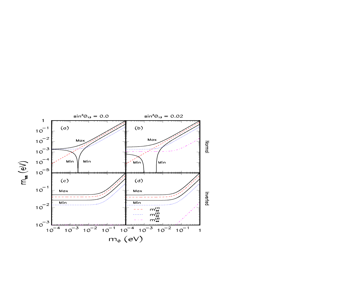
Figure 2: Maximum and minimum possible values of $m_{ee}$ as a function of $m_{0}$ indicated by the thick solid curves for $\sin^{2}\theta_{13}=0$ (left panels) and 0.02 (right panels) for normal (upper panels) as well as for inverted (lower panels) mass ordering. We have fixed the other mixing parameters as $\Delta m^{2}_{12}=5\times 10^{-5}$ eV², $\tan^{2}\theta_{12}$ = 0.35 and $|\Delta m^{2}_{23}|=3\times 10^{-3}$ eV². The individual contributions of $m_{ee}^{(1)}$, $m_{ee}^{(2)}$ and $m_{ee}^{(3)}$ are also shown by dashed, dotted and dash-dotted curves, respectively.

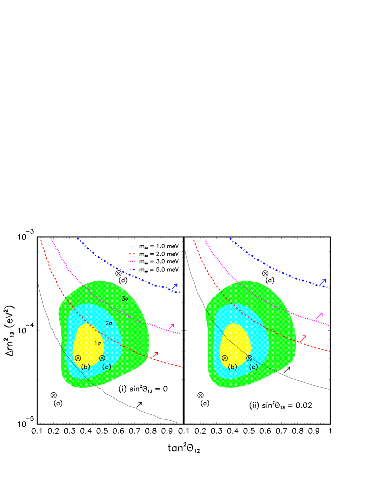
Figure 6: Region in the ($\Delta m^{2}_{12}$, $\tan^{2}\theta_{12}$) plane where $\alpha_{1}$ can be constrained to a non-zero value, indicated by an arrow, for given central values of $m_{ee}=1,2,3$ meV, taking into account 30% uncertainty in the determination of $m_{ee}$ and 10 % uncertainty in $\Delta m^{2}_{12}$ as well as in $\tan^{2}\theta_{12}$. The set of solar parameters used in Fig. 3(a)-(d) are indicated by crosses. The allowed region for the LMA MSW solution at 1, 2 and 3 $\sigma$ are shown by the shaded area (adopted from Ref. Holanda ).

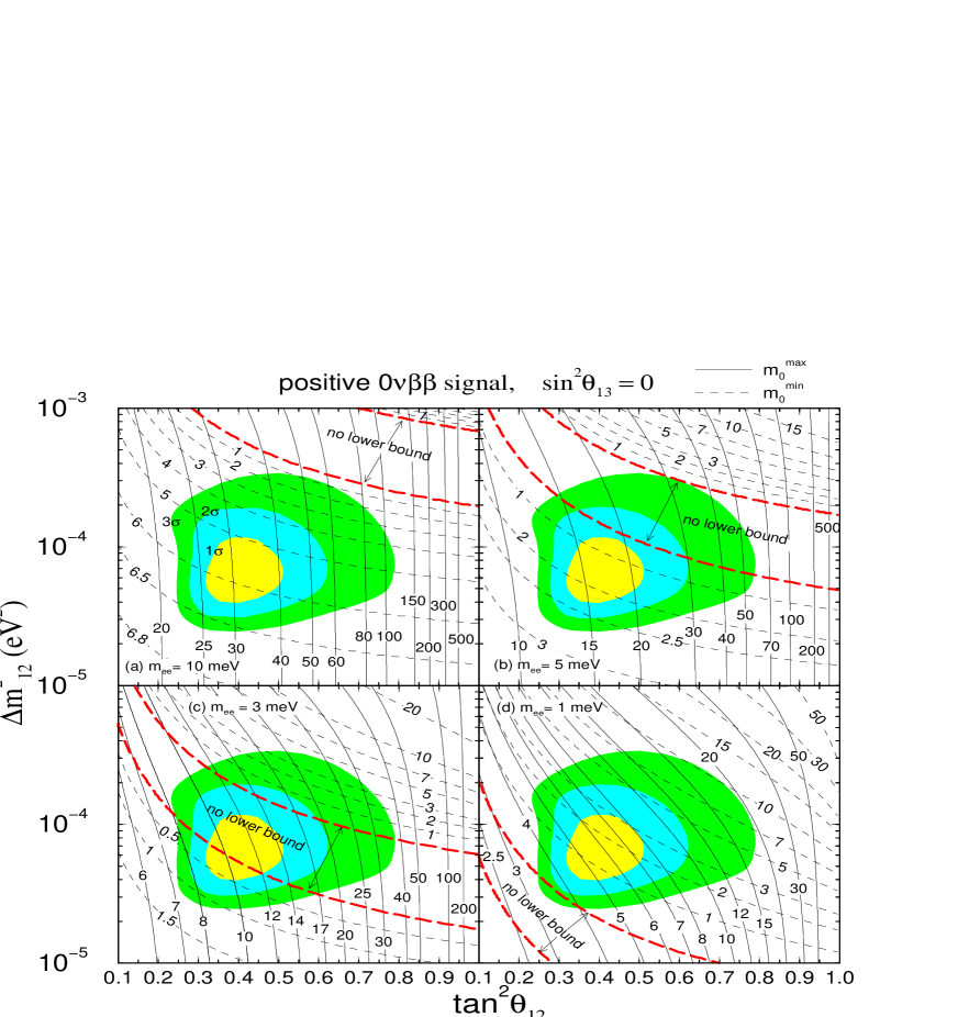
Figure 8: Iso-contour plots of upper ($m_{0}^{\text{max}}$, solid curves) and lower ($m_{0}^{\text{min}}$, dashed curves) bounds of $m_{0}$ in units of meV in the $\tan^{2}\theta_{12}-\Delta m^{2}_{12}$ plane for the case where a positive signal of $0\nu\beta\beta$ is observed with central values, $m_{ee}$ = 10 meV (a), 5 meV (b), 3 meV (c) and 1 meV (d). We assume 30% uncertainty in the determination of $m_{ee}$. We fix the other mixing parameters as $\Delta m^{2}_{23}=3\times 10^{-3}$ eV² and $\sin^{2}\theta_{13}=0$. The allowed region for the LMA MSW solution is the same as in Fig. 6.

- (1) Q. R. Ahmad et al. (SNO Collaboration), Phys. Rev. Lett. 87, 071301 (2001); S. Fukuda et al. (Super-Kamiokande Collaboration), Phys. Rev. Lett. 86, 5651 (2001); ibid. 86, 5656 (2001); arXiv:hep-ex/0205075; K. Lande et al. (Homestake Collaboration), Astrophys .J. 496, 505 (1998); J. Abdurashitov et al. (SAGE Collaboration), Phys. Rev. C 60, 055801 (1999); W. Hampel et al. (GALLEX Collaboration), Phys. Lett. B 447, 127 (1999); M. Altmann et al. (GNO Collaboration), Phys. Lett. B 490, 16 (2000).
- (2) Y. Fukuda et al. (Super-Kamiokande Collaboration), Phys. Rev. Lett. 81, 1562 (1998); H. S. Hirata et al. (Kamiokande Collaboration), Phys. Lett. B 205, 416 (1988); ibid. 280, 146 (1992); Y. Fukuda et al., ibid. 335, 237 (1994); R. Becker-Szendy et al. (IMB Collaboration), Phys. Rev. D 46, 3720 (1992); M. Ambrosio et al. (MACRO Collaboration), Phys. Lett. B 478, 5 (2000); B. C. Barish, Nucl. Phys. B (Proc. Suppl.) 91, 141 (2001); W. W. M. Allison et al. (Soudan-2 Collaboration), Phys. Lett. B 391, 491 (1997); Phys. Lett. B 449, 137 (1999); W. A. Mann, Nucl. Phys. B (Proc. Suppl.) 91, 134 (2001);
- (3) Q. R. Ahmad et al. (SNO Collaboration), arXiv:nucl-ex/0204008, arXiv:nucl-ex/0204009.
- (4) S. H. Ahn et al. (K2K Collaboration), Phys. Lett. B 511, 178 (2001); J. E. Hill (K2K Collaboration), in Proc. of the APS/DPF/DPB Summer Study on the Future of Particle Physics (Snowmass 2001) ed. by R. Davidson and C. Quigg, arXiv:hep-ex/0110034.
- (5) M. Apollonio et al. (CHOOZ Collaboration), Phys. Lett. B 420, 397 (1998); ibid. 466, 415 (1999); F. Boehm et al. (Palo Verde Collaboration), Phys. Rev. D 62, 072002 (2000); Phys. Rev. D 64, 112001 (2001).
- (6) Z. Maki, M. Nakagawa, and S. Sakata, Prog. Theor. Phys. 28, 870 (1962).
- (7) H. Minakata and H. Nunokawa, JHEP 0110, 001 (2001), V. Barger et al., Phys. Rev. D 65, 053016 (2002); T. Kajita, H. Minakata and H. Nunokawa, Phys. Lett. B 528, 245 (2002); M. Aoki et al., arXiv:hep-ph/0112338; P. Huber, M. Lindner and W. Winter, arXiv:hep-ph/0204352; A. Donini, D. Meloni and P. Migliozzi, arXiv:hep-ph/0206034; V. Barger, D. Marfatia and K. Whisnant, arXiv:hep-ph/0206038; G. Barenboim et al., arXiv:hep-ph/0204208; arXiv:hep-ph/0206025.
- (8) V. Barger, D. Marfatia and B. P. Wood, Phys. Lett. B 498, 53 (2001); H. Murayama and A. Pierce, Phys. Rev. D 65, 013012 (2002); A. de Gouvea and C. Pena-Garay, Phys. Rev. D 65, 0113011 (2001); M. C. Gonzalez-Garcia and C. Pena-Garay, Phys. Lett. B 527, 199 (2002); P. Aliani et al., arXiv:hep-ph/0205061.
- (9) J. Schechter and J. W. Valle, Phys. Rev. D 22, 2227 (1980); ibid. 23, 1666 (1981); ibid. 24, 1883 (1981); [Erratum-ibid. D 25, 283 (1982)].
- (10) S. M. Bilenky, J. Hosek and S. T. Petcov, Phys. Lett. B 94, 495 (1980).
- (11) M. Doi et al., Phys. Lett. B 102, 323 (1981).
- (12) M. Doi, T. Kotani and E. Takasugi, Prog. Theor. Phys. Suppl. 83, 1 (1985); T. Tomoda, Rep. Prog. Phys. 54, 53 (1991).
- (13) J. Schechter and J. W. F. Valle, Phys. Rev. D 25, 2951 (1982).
- (14) M. Hirsch, H. V. Klapdor-Kleingrothaus and S. G. Kovalenko, Phys. Rev. Lett. 75, 17 (1995); Phys. Rev. D 53, 1329 (1996); M. Hirsch and J. W. F. Valle, Nucl. Phys. B 557, 60 (1999).
- (15) S. T. Petcov and A. Yu. Smirnov, Phys. Lett. B 322, 109 (1994); S. M. Bilenky, C. Giunti, C. W. Kim and S. T. Petcov, Phys. Rev. D 54, 4432 (1996) H. Minakata and O. Yasuda, Phys. Rev. D 56, 1692 (1997); H. Minakata and O. Yasuda, Nucl. Phys. B 523, 597 (1998); T. Fukuyama, K. Matsuda and H. Nishiura, Phys. Rev. D 57, 5844 (1998); ibid. 81, 4279 (1998); F. Vissani, JHEP 9906, 022 (1999); S. M. Bilenky et al., Phys. Lett. B 465, 193 (1999); K. Matsuda et al., Phys. Rev. D 62, 093001 (2000); H. V. Klapdor-Kleingrothaus, H. Päs and A. Yu. Smirnov, Phys. Rev. D 63, 073005 (2001); W. Rodejohann, Nucl. Phys. B 597, 110 (2001); Y. Farzan, O. L. G. Peres and A. Yu. Smirnov, Nucl. Phys. B 612, 59 (2001); S. M. Bilenky, S. Pascoli and S. T. Petcov, Phys. Rev. D 64, 053010 (2001); H. Minakata and H. Sugiyama, Phys. Lett. B 526, 335 (2002); ibid. 532, 275 (2002); . Falcone and F. Tramontano, Phys. Rev. D 64, 077302 (2001); Z. z. Xing, Phys. Rev. D 65, 077302 (2002); H. J. He, D. A. Dicus and J. N. Ng, Phys. Lett. B 536, 83 (2002) S. Pascoli, S. T. Petcov and L. Wolfenstein, Phys. Lett. B 524, 319 (2002) W. Rodejohann, arXiv:hep-ph/0203214; F. Feruglio, A. Strumia and F. Vissani, arXiv:hep-ph/0201291, to appear in Nucl. Phys. B; S. Pascoli and S. T. Petcov, arXiv:hep-ph/0205022; S. Pascoli and S. T. Petcov, arXiv:hep-ph/0111203.
- (16) For instance, the following articles also discussed and demonstrated the relation between decay signal and the absolute neutrino mass scales and/or Majorana CP phases but in different ways from the ones we consider in this work: V. Barger and K. Whisnant, Phys. Lett. B 456, 194 (1999); H. Päs and T. J. Weiler, Phys. Rev. D 63, 113015 (2001); P. Osland and G. Vigdel, Phys. Lett. B 520, 143 (2001); V. Barger et al., Phys. Lett. B 532, 15 (2002); M. Frigerio and A. Yu. Smirnov, arXiv:hep-ph/0202247.
- (17) H. V. Klapdor-Kleingrothaus et al. (Heidelberg–Moscow Collaboration), Eur. Phys. J. A 12, 147 (2001); see also C. E. Aalseth et al. (16EX Collaboration), arXiv:hep-ex/0202026.
- (18) H. V. Klapdor-Kleingrothaus et al., Mod. Phys. Lett. A 16, 2409 (2001).
- (19) C. E. Aalseth et al., arXiv:hep-ex/0202018; H. V. Klapdor-Kleingrothaus, arXiv:hep-ph/0205288; H. L. Harney, arXiv:hep-ph/0205293.
- (20) H. V. Klapdor-Kleingrothaus et al. (GENIUS Collaboration), arXiv:hep-ph/9910205.
- (21) E. Fiorini et al., Phys. Rep. 307, 309 (1998); A. Bettini, Nucl. Phys. Proc. Suppl. 100, 332 (2001).
- (22) M. Danilov et al., Phys. Lett. B 480, 12 (2000).
- (23) C. E. Aalseth et al. (MAJORANA Collaboration), arXiv:hep-ex/0201021.
- (24) H. Ejiri et al., Phys. Rev. Lett. 85, 2917 (2000).
- (25) J. Bonn et al., (Mainz Collaboration), Nucl. Phys. Proc. Suppl. 91, 273 (2001).
- (26) A. Osipowicz et al. (KATRIN Collaboration), arXiv:hep-ex/0109033.
- (27) G. L. Fogli et al., Phys. Rev. D 64, 093007 (2001); A. M. Gago et al., Phys. Rev. D 65, 073012 (2002); J. N. Bahcall et al., arXiv:hep-ph/0204314; A. Bandyopadhyay et al., arXiv:hep-ph/0204286 V. Barger et al., arXiv:hep-ph/0204253; P. C. de Holanda and A. Yu. Smirnov arXiv:hep-ph/0205241; P. Creminelli et al., arXiv:hep-ph/0102234.
- (28) For a recent review on decay, see S. R. Elliot and P. Vogel, arXiv:hep-ph/0202264.
- (29) V. Barger et al., arXiv:hep-ph/0205290.
- (30) See P. C. de Holanda and A. Yu. Smirnov in Ref sol-recent .
- (31) See http://map.gsfc.nasa.gov/
- (32) See http://astro.estec.esa.nl/SA-general/Projects/Planck/.
- (33) W. Hu, D. J. Eisenstein and M. Tegmark, Phys. Rev. Lett. 80, 5255 (1998); M. Tegmark, M. Zaldarriaga and A. J. Hamilton, Nucl. Phys. Proc. Suppl. 91, 38 (2001).
- (34) T. Totani, Phys. Rev. Lett. 80, 2039 (1998); J. F. Beacom, R. N. Boyd and A. Mezzacappa, Phys. Rev. Lett. 85, 3568 (2000).