hep-ph/0206136

Fermilab-Pub-02/118-T

Two-loop effective potential for the minimal supersymmetric standard model

Stephen P. Martin

Department of Physics, Northern Illinois University, DeKalb IL 60115 $\rm and$
Fermi National Accelerator Laboratory, P.O. Box 500, Batavia IL 60510

I compute the complete two-loop effective potential for the minimal supersymmetric standard model in the Landau gauge. This enables an accurate determination of the minimization conditions for the vacuum expectation values of the Higgs fields. Checks on the result follow from supersymmetric limits and from renormalization-scale invariance. The renormalization group equations for the field-independent vacuum energy and the vacuum expectation values are also presented. I provide numerical examples showing the improved accuracy and scale dependence obtained with the full two-loop effective potential.

1 Introduction

The mechanism of electroweak symmetry breaking will be the principal focus of experimental investigations at the high-energy frontier for the next decade. Supersymmetry provides a highly predictive mechanism for addressing the hierarchy problem associated with the electroweak symmetry breaking scale. If supersymmetry is correct, then interpretations of future experimental data will rely on precise theoretical calculations in candidate models of supersymmetry breaking. The effective potential [2]-[4] approach allows the computation of the vacuum expectation values (VEVs) of Higgs fields in terms of the underlying Lagrangian parameters of a given theory.

The scalar potential of the Minimal Supersymmetric Standard Model (MSSM; for reviews, see [5]-[7]) is notoriously sensitive to radiative corrections. At tree level, the Higgs field quartic couplings are proportional to a sum of squares of electroweak gauge couplings and are therefore known not to be very large. Furthermore, they actually vanish along a $D$-flat direction in field space. These facts ensures the existence of at least one light Higgs scalar boson, corresponding to a shallow direction in the effective potential for the Higgs vacuum expectation values. The same facts also imply that the minimization conditions for the scalar potential depend very significantly on radiative corrections.

Previous results for the effective potential in the MSSM have included the full one-loop contributions [8] and partial two-loop corrections [9]-[12] including the effects of the QCD coupling and the top and bottom Yukawa couplings. Including these contributions mitigates the scale-dependence of the tree-level effective potential. However, I find that there is still a significant scale dependence and overall error compared to the uncertainties in theoretical quantities that may eventually be obtained at future experiments, especially at a linear $e^{+}e^{-}$ collider. In this paper, I will present the result for the full two-loop effective potential of the MSSM, in the Landau gauge and in the $\overline{\rm DR}^{\prime}$ [13] regularization and renormalization scheme. This is an application of the results given in ref. [14] for a general field theory. The $\overline{\rm DR}^{\prime}$ scheme is the variant of the $\overline{\rm DR}$ scheme [15] in which the effects of unphysical epsilon-scalars masses are removed by parameter redefinitions [13, 14].

The two-loop effective potential for a general renormalizable theory can be written as

$$V_{\rm eff}=V^{(0)}+{1\over 16\pi^{2}}V^{(1)}+{1\over(16\pi^{2})^{2}}V^{(2)}.$$ (1.1)

Here $V^{(0)}$ is the tree-level contribution. In the $\overline{\rm DR}^{\prime}$ scheme, the one-loop contribution is

$$V^{(1)}=\sum_{n}(-1)^{2s_{n}}(2s_{n}+1)h(m_{n}^{2}),$$ (1.2)

where $s_{n}=0,1/2,1$ for real scalars, two-component fermions, and vector fields, respectively, with field-dependent tree-level squared masses $m_{n}^{2}$. The one-loop function is

$$h(x)={x^{2}\over 4}\left[{\rm ln}(x/Q^{2})-3/2\right],$$ (1.3)

where $Q$ is the renormalization scale. The two-loop contribution always has the form

$$V^{(2)}=\sum_{n,p}\lambda^{nnpp}F_{np}(m_{n}^{2},m_{p}^{2})+\sum_{n,p,q}|\lambda^{npq}|^{2}F_{npq}(m_{n}^{2},m_{p}^{2},m_{q}^{2}),$$ (1.4)

where $\lambda^{npqr}$ and $\lambda^{npq}$ are tree-level field-dependent four- and three-particle couplings, and $F_{np}$ and $F_{npq}$ are $Q$-dependent functions of the $m_{n}^{2}$, depending on the particle types. The two-loop functions can be evaluated analytically using various methods developed in [16]-[20]. In general, one can write the results in terms of 10 basis functions, corresponding to the one-particle-irreducible connected vacuum graphs shown in Figure 1. These functions were given explicitly in ref. [14].

1

Figure 1: The one-particle-irreducible connected Feynman diagrams contributing to the two-loop effective potential. Dashed lines denote real scalars, solid lines denote Weyl fermions carrying helicity along the arrow direction, wavy lines are for vector bosons, and dotted lines are for ghosts. The large dots between opposing arrows on the fermion lines in the $\overline{FF}S$ and $\overline{FF}V$ diagrams denote mass insertions. The $\overline{FF}S$ diagram is accompanied by its complex conjugate (the same diagram with all arrows reversed). The effects of the VV, VVV, and ggV diagrams can always be combined into a “gauge” contribution. The loop integral functions associated with these Feynman diagrams are given explicitly in ref. [14].

In the MSSM, there are two Higgs VEVs, $v_{u}$ and $v_{d}$. The evaluation of the two-loop effective potential as a function of the VEVs reduces to determination of the relevant tree-level field-dependent couplings and masses. I will do this in the approximation of no Yukawa or flavor-violating couplings for the first two families of (s)quarks and (s)leptons. However, all remaining complex phases which cannot be rotated away are maintained. The resulting expressions presented here are complicated, but suitable for direct evaluation by computer programs.

The rest of this paper is organized as follows. In section 2, I describe necessary conventions and define some coefficients used in the calculation. Section 3 contains the expressions for the effective potential in the MSSM up to two-loop order. Section 4 discusses supersymmetric limits of the effective potential. In section 5, I present two-loop results for the Higgs scalar anomalous dimensions and the beta function of the vacuum energy. These are necessary for checking the scale-independence of the effective potential. Section 6 treats a numerical example.

2 Conventions and setup

In this section, I list the necessary facts and conventions used in this paper. The MSSM is a softly-broken supersymmetric theory, with $SU(3)_{c}\times SU(2)_{L}\times U(1)_{Y}$ gauge couplings $g_{3}$, $g$, and $g^{\prime}$. The last is related to the GUT normalized coupling $g_{1}$ by $g^{\prime}=\sqrt{{3/5}}\,g_{1}$. The superpotential of the MSSM is:

$$W=\overline{u}{\bf Y}_{u}QH_{u}-\overline{d}{\bf Y}_{d}QH_{d}-\overline{e}{\bf Y}_{e}LH_{d}+\mu H_{u}H_{d},$$ (2.1)

where $H_{u}$ and $H_{d}$ are the Higgs chiral superfields, and the $Q,L$ are the chiral superfields containing left-handed quarks and leptons and $u,d,e$ are those containing the conjugates of the right-handed quarks and leptons. The quark and lepton superfields carry a suppressed family index, so that ${\bf Y}_{u}$, ${\bf Y}_{d}$, ${\bf Y}_{e}$ are $3\times 3$ matrices in family space. Gauge indices for $SU(2)_{L}$ and $SU(3)_{c}$ are also suppressed, as in ref. [7]. The Higgs mass parameter $\mu$ can have an arbitrary phase. The soft supersymmetry-breaking part of the Lagrangian is:

$$-{\cal L}_{\rm soft} = \Bigl{(}{1\over 2}M_{1}\widetilde{B}\widetilde{B}+{1\over 2}M_{2}\widetilde{W}\widetilde{W}+{1\over 2}M_{3}\widetilde{g}\widetilde{g}$$ (2.2)

$$+\overline{u}{\bf a}_{u}QH_{u}-\overline{d}{\bf a}_{d}QH_{d}-\overline{e}{\bf a}_{e}LH_{d}+bH_{u}H_{d}\Bigr{)}+{\rm c.c.}$$

$$+m^{2}_{H_{u}}|H_{u}|^{2}+m^{2}_{H_{d}}|H_{d}|^{2}$$

$$+Q^{\dagger}{\bf m}^{2}_{Q}Q+L^{\dagger}{\bf m}^{2}_{L}L+\overline{u}{\bf m}^{2}_{u}\overline{u}^{\dagger}+\overline{d}{\bf m}^{2}_{d}\overline{d}^{\dagger}+\overline{e}{\bf m}^{2}_{e}\overline{e}^{\dagger}.$$

where $\widetilde{B}$, $\widetilde{W}$, and $\widetilde{g}$ are the bino, wino, and gluino fields, and the same symbols are used for scalar fields as for the corresponding superfields. Here, ${\bf a}_{u}$, ${\bf a}_{d}$, ${\bf a}_{e}$ are scalar cubic couplings in the form of $3\times 3$ matrices in family space. The Higgs fields have soft supersymmetry-breaking squared-mass running parameters $m_{H_{u}}^{2}$, $m_{H_{d}}^{2}$, and $b$. The first two of these are necessarily real, and by convention $b$ is taken to be real at the renormalization scale $Q$ at which the effective potential is to be minimized. This can always be achieved by a suitable field rephasing, and ensures that the VEVs obtained by minimizing the full effective potential will also be real. The squarks and sleptons have running soft supersymmetry-breaking squared masses ${\bf m}^{2}_{Q}$, ${\bf m}^{2}_{L}$, ${\bf m}^{2}_{u}$, ${\bf m}^{2}_{d}$, and ${\bf m}^{2}_{e}$, which are $3\times 3$ Hermitian matrices in flavor space.

The gauge-eigenstate complex scalar doublet Higgs fields that are components of left-handed chiral superfields are called $H_{u}=(H_{u}^{+},H_{u}^{0})$ and $H_{d}=(H_{d}^{0},H_{d}^{-})$. The electrically-neutral components have real positive VEVs $v_{u}$ and $v_{d}$ respectively. The field-dependent tree-level squared masses for vector bosons are then given by

$$m^{2}_{W} = {g^{2}\over 2}(v_{u}^{2}+v_{d}^{2});$$ (2.3)

$$m^{2}_{Z} = {g^{2}+g^{\prime 2}\over 2}(v_{u}^{2}+v_{d}^{2}).$$ (2.4)

The tree-level Higgs potential is

$$V\! = \!\Lambda+(|\mu|^{2}+m^{2}_{H_{u}})(|H_{u}^{0}|^{2}+|H_{u}^{+}|^{2})+(|\mu|^{2}+m^{2}_{H_{d}})(|H_{d}^{0}|^{2}+|H_{d}^{-}|^{2})$$ (2.5)

$$+\,b\,(H_{u}^{+}H_{d}^{-}-H_{u}^{0}H_{d}^{0})+{\rm c.c.}$$

$$+{1\over 8}(g^{2}+g^{\prime 2})(|H_{u}^{0}|^{2}+|H_{u}^{+}|^{2}-|H_{d}^{0}|^{2}-|H_{d}^{-}|^{2})^{2}+{g^{2}\over 2}|H_{u}^{+}H_{d}^{0*}+H_{u}^{0}H_{d}^{-*}|^{2}.$$

Here $\Lambda$ is a running field-independent vacuum energy, which must be included to maintain renormalization-scale independence of the effective potential [21]-[24]. The neutral Higgs scalar tree-level squared masses are obtained by diagonalizing the matrices:

$$m^{2}_{\phi_{R}^{0}} = \pmatrix{|\mu|^{2}+m^{2}_{H_{u}}+{g^{2}+g^{\prime 2}\over 4}(3v_{u}^{2}-v_{d}^{2})&-b-({g^{2}+g^{\prime 2}})v_{u}v_{d}/2\cr-b-({g^{2}+g^{\prime 2}})v_{u}v_{d}/2&|\mu|^{2}+m^{2}_{H_{d}}+{g^{2}+g^{\prime 2}\over 4}(3v_{d}^{2}-v_{u}^{2})};$$ (2.6)

$$m^{2}_{\phi_{I}^{0}} = \pmatrix{|\mu|^{2}+m^{2}_{H_{u}}+{g^{2}+g^{\prime 2}\over 4}(v_{u}^{2}-v_{d}^{2})&b\cr b&|\mu|^{2}+m^{2}_{H_{d}}+{g^{2}+g^{\prime 2}\over 4}(v_{d}^{2}-v_{u}^{2})},$$ (2.7)

which are written in the $({\rm Re}[H_{u}^{0}],{\rm Re}[H_{d}^{0}])$ and $({\rm Im}[H_{u}^{0}],{\rm Im}[H_{d}^{0}])$ bases, respectively. The complex charge $\pm 1$ Higgs scalar tree-level squared masses are obtained by diagonalizing the matrix

$$m^{2}_{\phi^{\pm}}=\pmatrix{|\mu|^{2}+m^{2}_{H_{u}}+{g^{2}+g^{\prime 2}\over 4}v_{u}^{2}+{g^{2}-g^{\prime 2}\over 4}v_{d}^{2}&b+{g^{2}}v_{u}v_{d}/2\cr b+{g^{2}}v_{u}v_{d}/2&|\mu|^{2}+m^{2}_{H_{d}}+{g^{2}+g^{\prime 2}\over 4}v_{d}^{2}+{g^{2}-g^{\prime 2}\over 4}v_{u}^{2}},$$ (2.8)

which is written in the $(H_{u}^{+},H_{d}^{-*})$ basis. The gauge-eigenstate fields can be expressed in terms of the tree-level squared-mass eigenstate fields as:

$$\pmatrix{H_{u}^{0}\cr H_{d}^{0}} = \pmatrix{v_{u}\cr v_{d}}+{1\over\sqrt{2}}{R}_{\alpha}\pmatrix{h^{0}\cr H^{0}}+{i\over\sqrt{2}}{R_{\beta_{0}}}\pmatrix{G^{0}\cr A^{0}}$$ (2.9)

and

$$\pmatrix{H_{u}^{+}\cr H_{d}^{-*}}={R}_{\beta_{\pm}}\pmatrix{G^{+}\cr H^{+}},$$ (2.10)

where $G^{0}$ and $G^{\pm}$ are Nambu-Goldstone fields, $h^{0},H^{0},A^{0}$, and $H^{\pm}$ are the physical Higgs tree-level mass-eigenstate fields, and

$${R}_{\alpha}=\pmatrix{c_{\alpha}&s_{\alpha}\cr-s_{\alpha}&c_{\alpha}};\qquad\qquad\!\!\!{R}_{\beta_{0}}=\pmatrix{s_{\beta_{0}}&c_{\beta_{0}}\cr-c_{\beta_{0}}&s_{\beta_{0}}};\qquad\qquad\!\!\!{R}_{\beta_{\pm}}=\pmatrix{s_{\beta_{\pm}}&c_{\beta_{\pm}}\cr-c_{\beta_{\pm}}&s_{\beta_{\pm}}}$$ (2.11)

are orthogonal matrices determined by the requirements that:

$${R}_{\alpha}^{-1}{m^{2}_{\phi_{R}^{0}}}R_{\alpha} = \pmatrix{m_{h^{0}}^{2}&0\cr 0&m_{H^{0}}^{2}};$$ (2.12)

$${R}_{\beta_{0}}^{-1}{m^{2}_{\phi_{I}^{0}}}R_{\beta_{0}} = \pmatrix{m_{G^{0}}^{2}&0\cr 0&m_{A^{0}}^{2}};$$ (2.13)

$$R_{\beta_{\pm}}^{-1}{m^{2}_{\phi^{\pm}}}R_{\beta_{\pm}} = \pmatrix{m_{G^{\pm}}^{2}&0\cr 0&m_{H^{\pm}}^{2}}.$$ (2.14)

These equations define the tree-level squared mass eigenvalues for the Higgs scalar sector and the mixing angles $\alpha$, $\beta_{0}$ and $\beta_{\pm}$. Here I use a notation in which $c$ and $s$ with a subscript indicate the cosine and sine of the indicated angle. So, in accord with the orthogonality of the rotation matrices, $c_{\alpha}$ means $\cos\alpha$, etc. Similarly, in the following, $c_{2\alpha}$ is taken to mean $\cos(2\alpha)$, and so on. Also, for future convenience, define coefficients

$$k_{uh^{0}}=k_{dH^{0}}=c_{\alpha};\qquad\qquad k_{uH^{0}}=-k_{dh^{0}}=s_{\alpha};$$ (2.15)

$$k_{uG^{0}}=k_{dA^{0}}=is_{\beta_{0}};\qquad\qquad k_{uA^{0}}=-k_{dG^{0}}=ic_{\beta_{0}};$$ (2.16)

$$k_{uG^{+}}=k_{dH^{+}}=s_{\beta_{\pm}};\qquad\qquad k_{uH^{+}}=-k_{dG^{+}}=c_{\beta_{\pm}}.$$ (2.17)

Conventionally, $c_{\alpha}$, $c_{\beta_{0}}$, and $c_{\beta_{\pm}}$ are taken to be positive. Because the minimum of the effective potential is not a minimum of the tree-level potential, the angles $\beta_{0}$ and $\beta_{\pm}$ for the rotations in the pseudo-scalar and charged Higgs sector are distinct from each other, and from $\beta=\tan^{-1}(v_{u}/v_{d})$ at the minimum of the effective potential. Some care should be used to distinguish these. Also, note that unlike the case in the ordinary Standard Model, $m_{G^{0}}^{2}\not=m_{G^{\pm}}^{2}$ at tree level. Note also that even with arbitrary CP-violating phases, there is no mixing in the tree-level squared masses of the neutral scalar $(h^{0},H^{0})$ and the pseudo-scalar $(G^{0},A^{0})$ sectors, because of the freedom to choose the argument of $b$ to be 0 at any particular renormalization scale $Q$.

In section 3, $\displaystyle\sum_{\phi^{0}}$ and $\displaystyle\sum_{\phi^{\pm}}$ will appear, denoting sums over the lists

$$\phi^{0}=(h^{0},H^{0},G^{0},A^{0})\qquad\mbox{and}\qquad\phi^{\pm}=(G^{\pm},H^{\pm})$$ (2.18)

respectively.

The neutralinos ($\tilde{N}_{i}$; $i=1,2,3,4$) and charginos ($\widetilde{C}_{i}^{\pm}$; $i=1,2$) are mixtures of the electroweak gaugino and Higgsino fields. In the $(\widetilde{B},\widetilde{W}^{0},\widetilde{H}_{d}^{0},\widetilde{H}_{u}^{0})$ gauge-eigenstate basis, the neutralino mass matrix is

$$M_{\tilde{N}}=\pmatrix{M_{1}&0&-g^{\prime}v_{d}/\sqrt{2}&g^{\prime}v_{u}/\sqrt{2}\cr 0&M_{2}&gv_{d}/\sqrt{2}&-gv_{u}/\sqrt{2}\cr-g^{\prime}v_{d}/\sqrt{2}&gv_{d}/\sqrt{2}&0&-\mu\cr g^{\prime}v_{u}/\sqrt{2}&-gv_{u}/\sqrt{2}&-\mu&0}.$$ (2.19)

This is diagonalized by a unitary matrix $N$:

$$N^{*}M_{\tilde{N}}N^{-1} = {\rm diag}(m_{\tilde{N}_{1}},m_{\tilde{N}_{2}},m_{\tilde{N}_{3}},m_{\tilde{N}_{4}}),$$ (2.20)

where the mass eigenvalues $m_{\tilde{N}_{i}}$ are all real and positive. This can always be accomplished (for any phases of $M_{1}$, $M_{2}$, and $\mu$) by the following procedure. First, define $E$ to be a matrix whose columns are orthonormal eigenvectors of the Hermitian squared-mass matrix $M_{\tilde{N}}^{\dagger}M_{\tilde{N}}$, arranged in order of increasing eigenvalue. The orthonormality means that $E^{\dagger}E=1$. It follows that

$$E^{T}M_{\tilde{N}}E = P^{2}m_{D},$$ (2.21)

where $m_{D}$ is the matrix on the right-hand side of eq. (2.20), and $P$ is a diagonal phase matrix. Then

$$N=PE^{\dagger}$$ (2.22)

satisfies eq. (2.20), and also

$$NM_{\tilde{N}}^{\dagger}M_{\tilde{N}}N^{-1}={\rm diag}(m^{2}_{\tilde{N}_{1}},m^{2}_{\tilde{N}_{2}},m^{2}_{\tilde{N}_{3}},m^{2}_{\tilde{N}_{4}}).$$ (2.23)

This procedure gives the tree-level field-dependent neutralino squared masses and mixing matrix $N_{ij}$. (A suitable generalization of this method can be used to transform the mass and squared-mass matrices into a real positive diagonal form for any fermions in any theory.)

The tree-level chargino mass matrix is given by

$$M_{\tilde{C}}=\pmatrix{M_{2}&gv_{u}\cr gv_{d}&\mu},$$ (2.24)

and is similarly diagonalized by unitary matrices $U$ and $V$ according to:

$$U^{*}M_{\tilde{C}}V^{\dagger} = \pmatrix{m_{\tilde{C}_{1}}&0\cr 0&m_{\tilde{C}_{2}}}$$ (2.25)

where again $m_{\tilde{C}_{i}}$ are real and positive. Then

$$VM_{\tilde{C}}^{\dagger}M_{\tilde{C}}V^{-1}=UM_{\tilde{C}}^{*}M_{\tilde{C}}^{T}U^{-1}=\pmatrix{m_{\tilde{C}_{1}}^{2}&0\cr 0&m_{\tilde{C}_{2}}^{2}}.$$ (2.26)

The tree-level squared mass of the gluino, denoted $m^{2}_{\tilde{g}}=|M_{3}|^{2}$, does not depend on the VEVs $v_{u}$ and $v_{d}$.

In most of this paper, I will employ the approximation that only the third-family Yukawa couplings $y_{t}$, $y_{b}$, and $y_{\tau}$ are significant, so that:

$${\bf Y}_{u}=\pmatrix{0&0&0\cr 0&0&0\cr 0&0&y_{t}};\qquad{\bf Y}_{d}=\pmatrix{0&0&0\cr 0&0&0\cr 0&0&y_{b}};\qquad{\bf Y}_{e}=\pmatrix{0&0&0\cr 0&0&0\cr 0&0&y_{\tau}}.$$ (2.27)

By suitable field redefinitions, they can be chosen real and positive. The non-zero quark and lepton squared masses are therefore:

$$m_{t}^{2}=y_{t}^{2}v_{u}^{2};\qquad\qquad m_{b}^{2}=y_{b}^{2}v_{d}^{2};\qquad\qquad m_{\tau}^{2}=y_{\tau}^{2}v_{d}^{2}.$$ (2.28)

(Effects of the other Yukawa couplings are certainly smaller than the dominant 3-loop order contributions.)

I will also assume here that the soft supersymmetry-breaking scalar cubic couplings involving first- and second-family sfermions vanish, so

$${\bf a}_{u}=\pmatrix{0&0&0\cr 0&0&0\cr 0&0&a_{t}};\qquad{\bf a}_{d}=\pmatrix{0&0&0\cr 0&0&0\cr 0&0&a_{b}};\qquad{\bf a}_{e}=\pmatrix{0&0&0\cr 0&0&0\cr 0&0&a_{\tau}},$$ (2.29)

and that, in the same basis, the soft supersymmetry-breaking scalar squared mass parameters are diagonal in family space, so

$${\bf m}^{2}_{Q}=\pmatrix{m^{2}_{Q_{1}}&0&0\cr 0&m^{2}_{Q_{2}}&0\cr 0&0&m^{2}_{Q_{3}}},\>\>{\rm etc.}$$ (2.30)

The parameters $a_{t}$, $a_{b}$, and $a_{\tau}$ can in general be complex, and $m^{2}_{Q_{1,2,3}}$ etc. are real soft running $\overline{\rm DR}^{\prime}$ squared mass parameters. The squared masses of the first-family squarks and sleptons are then given by:

$$m^{2}_{\tilde{u}_{L}}\!\! =\>m^{2}_{Q_{1}}+\Delta_{\tilde{u}_{L}};\qquad\qquad m^{2}_{\tilde{d}_{L}}\!\! =\>m^{2}_{Q_{1}}+\Delta_{\tilde{d}_{L}};$$ (2.31)

$$m^{2}_{\tilde{u}_{R}}\!\! =\>m^{2}_{u_{1}}+\Delta_{\tilde{u}_{R}};\qquad\qquad m^{2}_{\tilde{d}_{R}}\!\! =\>m^{2}_{d_{1}}+\Delta_{\tilde{d}_{R}};$$ (2.32)

$$m^{2}_{\tilde{\nu}_{e}}\!\! =\>m^{2}_{L_{1}}+\Delta_{\tilde{\nu}_{e}};\qquad\qquad m^{2}_{\tilde{e}_{L}}\!\! =\>m^{2}_{L_{1}}+\Delta_{\tilde{e}_{L}};$$ (2.33)

$$m^{2}_{\tilde{e}_{R}}\!\! =\>m^{2}_{e_{1}}+\Delta_{\tilde{e}_{R}},\phantom{m^{2}_{\tilde{\nu}_{e}}}\qquad\qquad$$ (2.34)

The $D$-term contributions are:

$$\Delta_{\tilde{f}} = {1\over 2}(I_{\tilde{f}}g^{2}-Y_{\tilde{f}}g^{\prime 2})(v_{d}^{2}-v_{u}^{2}),$$ (2.35)

with $I_{\tilde{f}}$ and $Y_{\tilde{f}}$ defined to be the third component of weak isospin and the weak hypercharge of the left-handed chiral superfield containing the squark or slepton $\widetilde{f}$:

	$\widetilde{u}_{L}$	$\widetilde{d}_{L}$	$\widetilde{\nu}_{e}$	$\widetilde{e}_{L}$	$\widetilde{u}_{R}$	$\widetilde{d}_{R}$	$\widetilde{e}_{R}$
$I_{\tilde{f}}$	$\phantom{-}1/2$	$-1/2$	$1/2$	$-1/2$	$0$	$\phantom{-1/}0$	$\phantom{-1/}0$
$Y_{\tilde{f}}$	$1/6$	$1/6$	$-1/2$	$-1/2$	$-2/3$	$1/3$	$1$

Exactly analogous expressions hold for the second-family squark and slepton squared masses $m^{2}_{\tilde{c}_{L}}$, $m^{2}_{\tilde{s}_{L}}$, $m^{2}_{\tilde{c}_{R}}$, $m^{2}_{\tilde{s}_{R}}$, $m^{2}_{\tilde{\nu}_{\mu}}$, $m^{2}_{\tilde{\mu}_{L}}$, and $m^{2}_{\tilde{\mu}_{R}}$, with the subscripts 1 replaced by 2 on the right-hand sides of eqs. (2.31)-(2.34).

For the stop, sbottom, stau, and stau-neutrino squared masses:

$$m^{2}_{\tilde{t}} = \pmatrix{m_{Q_{3}}^{2}+y_{t}^{2}v_{u}^{2}+\Delta_{\tilde{u}_{L}}&v_{u}a_{t}^{*}-v_{d}\mu y_{t}\cr v_{u}a_{t}-v_{d}\mu^{*}y_{t}&m_{u_{3}}^{2}+y_{t}^{2}v_{u}^{2}+\Delta_{\tilde{u}_{R}}};$$ (2.36)

$$m^{2}_{\tilde{b}} = \pmatrix{m_{Q_{3}}^{2}+y_{b}^{2}v_{d}^{2}+\Delta_{\tilde{d}_{L}}&v_{d}a_{b}^{*}-v_{u}\mu y_{b}\cr v_{d}a_{b}-v_{u}\mu^{*}y_{b}&m_{d_{3}}^{2}+y_{b}^{2}v_{d}^{2}+\Delta_{d_{R}}};$$ (2.37)

$$m^{2}_{\tilde{\tau}} = \pmatrix{m_{L_{3}}^{2}+y_{\tau}^{2}v_{d}^{2}+\Delta_{\tilde{e}_{L}}&v_{d}a_{\tau}^{*}-v_{u}\mu y_{\tau}\cr v_{d}a_{\tau}-v_{u}\mu^{*}y_{\tau}&m_{e_{3}}^{2}+y_{\tau}^{2}v_{d}^{2}+\Delta_{\tilde{e}_{R}}};$$ (2.38)

$$m^{2}_{\tilde{\nu}_{\tau}} = m_{\tilde{L}_{3}}^{2}+\Delta_{\tilde{\nu}_{e}}.$$ (2.39)

Here the stop, sbottom and stau squared mass matrices are given in the $(\widetilde{f}_{L},\widetilde{f}_{R})$ bases. The eigenvalues of eqs. (2.36)-(2.38) give the squared mass eigenvalues $m_{\tilde{t}_{i}}^{2}$, $m_{\tilde{b}_{i}}^{2}$, and $m_{\tilde{\tau}_{i}}^{2}$ for $i=1,2$. The squared-mass matrices are diagonalized by unitary transformations:

$$\pmatrix{\widetilde{f}_{L}\cr\widetilde{f}_{R}}=X_{\tilde{f}}\pmatrix{\widetilde{f}_{1}\cr\widetilde{f}_{2}}$$ (2.40)

for $f=t,b,\tau$, with

$$X_{\tilde{f}}=\pmatrix{L_{\tilde{f}_{1}}&L_{\tilde{f}_{2}}\cr R_{\tilde{f}_{1}}&R_{\tilde{f}_{2}}},$$ (2.41)

so that

$$X_{\tilde{t}}^{-1}m^{2}_{\tilde{t}}X_{\tilde{t}}=\pmatrix{m_{\tilde{t}_{1}}^{2}&0\cr 0&m^{2}_{\tilde{t}_{2}}},$$ (2.42)

and similarly for the sbottoms and staus. Unitarity of the matrix $X_{\tilde{f}}$ allows one to write $L_{\tilde{f}_{1}}=R_{\tilde{f}_{2}}^{*}=c_{\tilde{f}}$, and $R_{\tilde{f}_{1}}=-L_{\tilde{f}_{2}}^{*}=s_{\tilde{f}}$, with

$$|c_{\tilde{f}}|^{2}+|s_{\tilde{f}}|^{2}=1.$$ (2.43)

(If the off-diagonal elements of the squared mass matrix are real, then $c_{\tilde{f}}$ and $s_{\tilde{f}}$ are the sine and cosine of a sfermion mixing angle.) In the following, I will also make use of coefficients:

$$x_{\tilde{f}}\,=\,I_{\tilde{f}},\qquad\qquad(\tilde{f}=\>\mbox{first or second family sfermion});\phantom{xxx}$$ (2.44)

$$x_{\tilde{t}_{i}}={1\over 2}|L_{\tilde{t}_{i}}|^{2};\qquad\>\>\>\>\>x_{\tilde{b}_{i}}=-{1\over 2}|L_{\tilde{b}_{i}}|^{2};\qquad\>\>\>\>\>x_{\tilde{\nu}_{\tau}}={1\over 2};\qquad\>\>\>\>\>x_{\tilde{\tau}_{i}}=-{1\over 2}|L_{\tilde{\tau}_{i}}|^{2},\phantom{xxx}$$ (2.45)

and

$$x^{\prime}_{\tilde{f}}\,=\,Y_{\tilde{f}},\qquad\qquad(\tilde{f}=\>\mbox{first or second family sfermion});$$ (2.46)

$$x^{\prime}_{\tilde{t}_{i}}={1\over 6}|L_{\tilde{t}_{i}}|^{2}-{2\over 3}|R_{\tilde{t}_{i}}|^{2};\qquad\qquad\>\>\>x^{\prime}_{\tilde{b}_{i}}={1\over 6}|L_{\tilde{b}_{i}}|^{2}+{1\over 3}|R_{\tilde{b}_{i}}|^{2};$$ (2.47)

$$x^{\prime}_{\tilde{\tau}_{i}}=-{1\over 2}|L_{\tilde{\tau}_{i}}|^{2}+|R_{\tilde{\tau}_{i}}|^{2};\qquad\qquad\>\>\>x^{\prime}_{\tilde{\nu}_{\tau}}=-{1\over 2}.$$ (2.48)

When $\displaystyle\sum_{\tilde{f}}$ appears in section 3, it will denote a sum over the list

$$\tilde{f}=(\widetilde{u}_{L},\widetilde{d}_{L},\widetilde{u}_{R},\widetilde{d}_{R},\widetilde{\nu}_{e},\widetilde{e}_{L},\widetilde{e}_{R},\widetilde{c}_{L},\widetilde{s}_{L},\widetilde{c}_{R},\widetilde{s}_{R},\widetilde{\nu}_{\mu},\widetilde{\mu}_{L},\widetilde{\mu}_{R},\widetilde{t}_{1},\widetilde{t}_{2},\widetilde{b}_{1},\widetilde{b}_{2},\widetilde{\nu}_{\tau},\widetilde{\tau}_{1},\widetilde{\tau}_{2}).$$ (2.49)

The symbol

$$n_{\tilde{f}}=\left\{\begin{array}[]{ll}1,&\tilde{f}=\>\mbox{slepton}\\ 3,&\tilde{f}=\>\mbox{squark}\end{array}\right.$$ (2.52)

denotes the number of colors.

To summarize, evaluation of the effective potential can proceed as follows. At a renormalization scale $Q$, choose values for the set of input data consisting of the 33 $\overline{\rm DR}^{\prime}$ running parameters:

$$v_{u},\>v_{d},$$ (2.53)

$$g_{3},\>g,\>g^{\prime},\>y_{t},\>y_{b},\>y_{\tau},$$ (2.54)

$$m_{Q_{i}}^{2},\>m_{L_{i}}^{2},\>m_{u_{i}}^{2},\>m_{d_{i}}^{2},\>m_{e_{i}}^{2},\qquad(i=1,2,3)$$ (2.55)

$$m_{H_{u}}^{2},\>m_{H_{d}}^{2},\>b,\>\mu,$$ (2.56)

$$M_{3},\>M_{2},\>M_{1},\>a_{t},\>a_{b},\>a_{\tau},$$ (2.57)

of which the last 7 may be complex. Using the preceding protocols, evaluate the mixing parameters

$$\alpha,\>\beta_{0},\>\beta_{\pm},$$ (2.58)

$$N_{ij},\>U_{ij},\>V_{ij},$$ (2.59)

$$L_{\tilde{t}_{i}},\>R_{\tilde{t}_{i}},\>L_{\tilde{b}_{i}},\>R_{\tilde{b}_{i}},\>L_{\tilde{\tau}_{i}},\>R_{\tilde{\tau}_{i}},\phantom{xxxxxxx}$$ (2.60)

and the 39 distinct field-dependent tree-level squared masses:

$$m_{W}^{2},\>m_{Z}^{2},$$ (2.61)

$$m_{h^{0}}^{2},\>m_{H^{0}}^{2},\>m_{G^{0}}^{2},\>m_{A^{0}}^{2},\>m_{G^{\pm}}^{2},\>m_{H^{\pm}}^{2},$$ (2.62)

$$m_{\tilde{g}}^{2},\>m^{2}_{\tilde{N}_{i}},\>m^{2}_{\tilde{C}_{i}},$$ (2.63)

$$m_{t}^{2},m_{b}^{2},m_{\tau}^{2},$$ (2.64)

$$m_{\tilde{u}_{L}}^{2},\>m_{\tilde{d}_{L}}^{2},\>m_{\tilde{u}_{R}}^{2},\>m_{\tilde{d}_{R}}^{2},\>m_{\tilde{\nu}_{e}}^{2},\>m_{\tilde{e}_{L}}^{2},\>m_{\tilde{e}_{R}}^{2},$$ (2.65)

$$m_{\tilde{c}_{L}}^{2},\>m_{\tilde{s}_{L}}^{2},\>m_{\tilde{c}_{R}}^{2},\>m_{\tilde{s}_{R}}^{2},\>m_{\tilde{\nu}_{\mu}}^{2},\>m_{\tilde{\mu}_{L}}^{2},\>m_{\tilde{\mu}_{R}}^{2},$$ (2.66)

$$m_{\tilde{t}_{1}}^{2},\>m_{\tilde{t}_{2}}^{2},\>m_{\tilde{b}_{1}}^{2},\>m_{\tilde{b}_{2}}^{2},\>m_{\tilde{\nu}_{\tau}}^{2},\>m_{\tilde{\tau}_{1}}^{2},\>m_{\tilde{\tau}_{2}}^{2}.$$ (2.67)

These squared masses (and implicitly $Q$) then become arguments for the functions $F_{SSS}$, $F_{SS}$, $F_{FFS}$, $F_{\overline{FF}S}$, $F_{SSV}$, $F_{VS}$, $F_{VVS}$, $F_{FFV}$, $F_{\overline{FF}V}$, and $F_{\rm gauge}$ appearing in the next section, and defined explicitly in eqs. (2.17)-(2.22), (4.12)-(4.16), and (6.21)-(6.30) of ref. [14]. (For the sake of uniformity of notation, I use the symbols $F_{SSS}$, $F_{SS}$, $F_{FFS}$, $F_{\overline{FF}S}$, and $F_{SSV}$ in place of $f_{SSS}$, $f_{SS}$, $f_{FFS}$, $f_{\overline{FF}S}$, and $f_{SSV}$ for the functions which are the same in the $\overline{\rm MS}$ and $\overline{\rm DR}^{\prime}$ schemes. All two-loop functions used in the present paper are $\overline{\rm DR}^{\prime}$ ones.) To simplify the notation, I adopt the convention that the name of a particle is synonymous with its squared mass when appearing as an argument of one of these functions. So, for example, $F_{SSS}(h^{0},A^{0},G^{0})$ means $F_{SSS}(m_{h^{0}}^{2},m_{A^{0}}^{2},m_{G_{0}}^{2})$.

3 MSSM effective potential

3.1 Tree-level and one-loop contributions

The tree-level contribution to the effective potential for $v_{u}$ and $v_{d}$ is:

$$V^{(0)}=\Lambda+(|\mu|^{2}+m^{2}_{H_{u}})v_{u}^{2}+(|\mu|^{2}+m^{2}_{H_{d}})v_{d}^{2}-2bv_{u}v_{d}+{1\over 8}(g^{2}+g^{\prime 2})(v_{u}^{2}-v_{d}^{2})^{2}.$$ (3.1)

The one-loop contribution in the $\overline{\rm DR}^{\prime}$ scheme is:

$$V^{(1)} = \sum_{\phi^{0}}h(\phi^{0})+2\sum_{\phi^{\pm}}h(\phi^{\pm})+2\sum_{\tilde{f}}n_{\tilde{f}}h(\tilde{f})-2\sum_{i=1}^{4}h(\tilde{N}_{i})-4\sum_{i=1}^{2}h(\widetilde{C}_{i})$$ (3.2)

$$-16h(\widetilde{g})-12h(t)-12h(b)-4h(\tau)+3h(Z)+6h(W),$$

where $h(x)$ is the function defined in eq. (1.3), and the name of each particle is used to denote its squared mass.

3.2 $SSS$-diagram contributions

In this subsection, I list the contributions to the MSSM two-loop effective potential from diagrams with three scalar propagators. These all involve the function $F_{SSS}(x,y,z)$, with arguments $x,y,z$ equal to tree-level field-dependent scalar squared masses.

The contributions from diagrams with three Higgs scalar propagators are:

$$V^{(2)}_{\phi^{0}\phi^{0}\phi^{0}} = {(g^{2}+g^{\prime 2})^{2}\over 32}\Biggl{[}(c_{\alpha}v_{u}+s_{\alpha}v_{d})^{2}\biggl{\{}3c_{2\alpha}^{2}F_{SSS}(h^{0},h^{0},h^{0})+2s_{2\beta_{0}}^{2}F_{SSS}(h^{0},A^{0},G^{0})$$ (3.3)

$$+c_{2\beta_{0}}^{2}[F_{SSS}(h^{0},G^{0},G^{0})+F_{SSS}(h^{0},A^{0},A^{0})]\biggr{\}}$$

$$+(s_{\alpha}v_{u}-c_{\alpha}v_{d})^{2}\biggl{\{}3c_{2\alpha}^{2}F_{SSS}(H^{0},H^{0},H^{0})+2s_{2\beta_{0}}^{2}F_{SSS}(H^{0},A^{0},G^{0})$$

$$+c_{2\beta_{0}}^{2}[F_{SSS}(H^{0},G^{0},G^{0})+F_{SSS}(H^{0},A^{0},A^{0})]\biggr{\}}$$

$$+[s_{\alpha}(1-6c_{\alpha}^{2})v_{u}+c_{\alpha}(1-6s_{\alpha}^{2})v_{d}]^{2}F_{SSS}(h^{0},h^{0},H^{0})$$

$$+[s_{\alpha}(1-6c_{\alpha}^{2})v_{d}-c_{\alpha}(1-6s_{\alpha}^{2})v_{u}]^{2}F_{SSS}(h^{0},H^{0},H^{0})\Biggr{]}$$

and

$$V^{(2)}_{\phi^{0}\phi^{\pm}\phi^{\pm}}={1\over 16}\Biggl{\{}2\Bigl{[}g^{2}c_{2\beta_{\pm}}(s_{\alpha}v_{u}-c_{\alpha}v_{d})+g^{\prime 2}s_{2\beta_{\pm}}(c_{\alpha}v_{u}+s_{\alpha}v_{d})\Bigr{]}^{2}F_{SSS}(h^{0},G^{\pm},H^{\pm})$$

$$+2\Bigl{[}g^{2}c_{2\beta_{\pm}}(c_{\alpha}v_{u}+s_{\alpha}v_{d})-g^{\prime 2}s_{2\beta_{\pm}}(s_{\alpha}v_{u}-c_{\alpha}v_{d})\Bigr{]}^{2}F_{SSS}(H^{0},G^{\pm},H^{\pm})$$

$$+\Bigl{[}g^{2}(c_{\alpha}v_{u}-s_{\alpha}v_{d})+g^{2}s_{2\beta_{\pm}}(s_{\alpha}v_{u}-c_{\alpha}v_{d})-g^{\prime 2}c_{2\beta_{\pm}}(c_{\alpha}v_{u}+s_{\alpha}v_{d})\Bigr{]}^{2}F_{SSS}(h^{0},G^{\pm},G^{\pm})$$

$$+\Bigl{[}g^{2}(c_{\alpha}v_{u}-s_{\alpha}v_{d})-g^{2}s_{2\beta_{\pm}}(s_{\alpha}v_{u}-c_{\alpha}v_{d})+g^{\prime 2}c_{2\beta_{\pm}}(c_{\alpha}v_{u}+s_{\alpha}v_{d})\Bigr{]}^{2}F_{SSS}(h^{0},H^{\pm},H^{\pm})$$

$$+\Bigl{[}g^{2}(s_{\alpha}v_{u}+c_{\alpha}v_{d})-g^{2}s_{2\beta_{\pm}}(c_{\alpha}v_{u}+s_{\alpha}v_{d})-g^{\prime 2}c_{2\beta_{\pm}}(s_{\alpha}v_{u}-c_{\alpha}v_{d})\Bigr{]}^{2}F_{SSS}(H^{0},G^{\pm},G^{\pm})$$

$$+\Bigl{[}g^{2}(s_{\alpha}v_{u}+c_{\alpha}v_{d})+g^{2}s_{2\beta_{\pm}}(c_{\alpha}v_{u}+s_{\alpha}v_{d})+g^{\prime 2}c_{2\beta_{\pm}}(s_{\alpha}v_{u}-c_{\alpha}v_{d})\Bigr{]}^{2}F_{SSS}(H^{0},H^{\pm},H^{\pm})$$

$$+2g^{4}(c_{\beta_{0}}v_{u}-s_{\beta_{0}}v_{d})^{2}F_{SSS}(G^{0},G^{\pm},H^{\pm})+2g^{4}(s_{\beta_{0}}v_{u}+c_{\beta_{0}}v_{d})^{2}F_{SSS}(A^{0},G^{\pm},H^{\pm})\Biggr{\}}.$$ (3.4)

The contributions from diagrams with two sfermions and a neutral Higgs scalar are:

$$V^{(2)}_{\phi^{0}\tilde{f}\tilde{f}^{\prime}} = {1\over 2}\sum_{\phi^{0},\tilde{f},\tilde{f}^{\prime}}n_{\tilde{f}}|\lambda_{\phi^{0}\tilde{f}\tilde{f}^{\prime*}}|^{2}F_{SSS}(\phi^{0},\widetilde{f},\widetilde{f}^{\prime}).$$ (3.5)

The couplings involving first- and second-family sfermions, and the tau sneutrino, are non-zero only when $\widetilde{f}=\widetilde{f}^{\prime}$. They are given by:

$$\lambda_{\phi^{0}\tilde{f}\tilde{f}^{*}}={1\over\sqrt{2}}\left(I_{\tilde{f}}g^{2}-Y_{\tilde{f}}g^{\prime 2}\right){\rm Re}[k_{u\phi^{0}}v_{u}-k_{d\phi^{0}}v_{d}],$$ (3.6)

with $I_{\tilde{f}},Y_{\tilde{f}}$ defined in section 2. The remaining couplings for the third-family sfermions are:

$$\lambda_{\phi^{0}\tilde{t}_{i}\tilde{t}_{j}^{*}} = L_{\tilde{t}_{i}}L^{*}_{\tilde{t}_{j}}\lambda_{\phi^{0}\tilde{u}_{L}\tilde{u}_{L}^{*}}+R_{\tilde{t}_{i}}R^{*}_{\tilde{t}_{j}}\lambda_{\phi^{0}\tilde{u}_{R}\tilde{u}_{R}^{*}}-\sqrt{2}v_{u}y_{t}^{2}{\rm Re}[k_{u\phi^{0}}](L_{\tilde{t}_{i}}L^{*}_{\tilde{t}_{j}}+R_{\tilde{t}_{i}}R^{*}_{\tilde{t}_{j}})$$ (3.7)

$$-{1\over\sqrt{2}}(k_{u\phi^{0}}a_{t}-k_{d\phi^{0}}^{*}\mu^{*}y_{t})L_{\tilde{t}_{i}}R^{*}_{\tilde{t}_{j}}-{1\over\sqrt{2}}(k_{u\phi^{0}}^{*}a_{t}^{*}-k_{d\phi^{0}}\mu y_{t})R_{\tilde{t}_{i}}L^{*}_{\tilde{t}_{j}};$$

$$\lambda_{\phi^{0}\tilde{b}_{i}\tilde{b}_{j}^{*}} = L_{\tilde{b}_{i}}L^{*}_{\tilde{b}_{j}}\lambda_{\phi^{0}\tilde{d}_{L}\tilde{d}_{L}^{*}}+R_{\tilde{b}_{i}}R^{*}_{\tilde{b}_{j}}\lambda_{\phi^{0}\tilde{d}_{R}\tilde{d}_{R}^{*}}-\sqrt{2}v_{d}y_{b}^{2}{\rm Re}[k_{d\phi^{0}}](L_{\tilde{b}_{i}}L^{*}_{\tilde{b}_{j}}+R_{\tilde{b}_{i}}R^{*}_{\tilde{b}_{j}})$$ (3.8)

$$-{1\over\sqrt{2}}(k_{d\phi^{0}}a_{b}-k_{u\phi^{0}}^{*}\mu^{*}y_{b})L_{\tilde{b}_{i}}R^{*}_{\tilde{b}_{j}}-{1\over\sqrt{2}}(k_{d\phi^{0}}^{*}a_{b}^{*}-k_{u\phi^{0}}\mu y_{b})R_{\tilde{b}_{i}}L^{*}_{\tilde{b}_{j}};$$

$$\lambda_{\phi^{0}\tilde{\tau}_{i}\tilde{\tau}_{j}^{*}} = L_{\tilde{\tau}_{i}}L^{*}_{\tilde{\tau}_{j}}\lambda_{\phi^{0}\tilde{e}_{L}\tilde{e}_{L}^{*}}+R_{\tilde{\tau}_{i}}R^{*}_{\tilde{\tau}_{j}}\lambda_{\phi^{0}\tilde{e}_{R}\tilde{e}_{R}^{*}}-\sqrt{2}v_{d}y_{\tau}^{2}{\rm Re}[k_{d\phi^{0}}](L_{\tilde{\tau}_{i}}L_{\tilde{\tau}_{j}}^{*}+R_{\tilde{\tau}_{i}}R^{*}_{\tilde{\tau}_{j}})$$ (3.9)

$$-{1\over\sqrt{2}}(k_{d\phi^{0}}a_{\tau}-k_{u\phi^{0}}^{*}\mu^{*}y_{\tau})L_{\tilde{\tau}_{i}}R^{*}_{\tilde{\tau}_{j}}-{1\over\sqrt{2}}(k_{d\phi^{0}}^{*}a_{\tau}^{*}-k_{u\phi^{0}}\mu y_{\tau})R_{\tilde{\tau}_{i}}L^{*}_{\tilde{\tau}_{j}}.$$

The contributions from diagrams with two sfermions and a charged Higgs scalar are:

$$V^{(2)}_{\phi^{\pm}\tilde{f}\tilde{f}^{\prime}} = \sum_{\phi^{+},\tilde{f},\tilde{f}^{\prime}}n_{\tilde{f}}|\lambda_{\phi^{+}\tilde{f}\tilde{f}^{\prime*}}|^{2}F_{SSS}(\phi^{\pm},\widetilde{f},\widetilde{f}^{\prime}).$$ (3.10)

Here the non-zero couplings involving the first- and second-family sfermions are:

$$\lambda_{\phi^{+}\tilde{e}_{L}\tilde{\nu}_{e}^{*}}=\lambda_{\phi^{+}\tilde{\mu}_{L}\tilde{\nu}_{\mu}^{*}}=\lambda_{\phi^{+}\tilde{d}_{L}\tilde{u}_{L}^{*}}=\lambda_{\phi^{+}\tilde{s}_{L}\tilde{c}_{L}^{*}} = -{g^{2}\over 2}(k_{u\phi^{+}}v_{u}+k_{d\phi^{+}}v_{d}),$$ (3.11)

and those involving the third-family sfermions are:

$$\lambda_{\phi^{+}\tilde{b}_{i}\tilde{t}_{j}^{*}} = L_{\tilde{b}_{i}}L^{*}_{\tilde{t}_{j}}\left(\lambda_{\phi^{+}\tilde{d}_{L}\tilde{u}_{L}^{*}}+y_{t}^{2}v_{u}k_{u\phi^{+}}+y_{b}^{2}v_{d}k_{d\phi^{+}}\right)+R_{\tilde{b}_{i}}R^{*}_{\tilde{t}_{j}}y_{t}y_{b}(k_{d\phi^{+}}v_{u}+k_{u\phi^{+}}v_{d})$$ (3.12)

$$+L_{\tilde{b}_{i}}R^{*}_{\tilde{t}_{j}}(k_{u\phi^{+}}a_{t}+k_{d\phi^{+}}\mu^{*}y_{t})+R_{\tilde{b}_{i}}L^{*}_{\tilde{t}_{j}}(k_{d\phi^{+}}a_{b}^{*}+k_{u\phi^{+}}\mu y_{b});$$

$$\lambda_{\phi^{+}\tilde{\tau}_{i}\tilde{\nu}_{\tau}^{*}} = L_{\tilde{\tau}_{i}}\left(\lambda_{\phi^{+}\tilde{e}_{L}\tilde{\nu}_{e}^{*}}+y_{\tau}^{2}v_{d}k_{d\phi^{+}}\right)+R_{\tilde{\tau}_{i}}(k_{d\phi^{+}}a_{\tau}^{*}+k_{u\phi^{+}}\mu y_{\tau}).$$ (3.13)

3.3 $SS$-diagram contributions

In this subsection, I list the contributions to the MSSM two-loop effective potential which come from diagrams with two scalar field propagators. They all involve the function $F_{SS}(x,y)$.

The contributions proportional to $g_{3}^{2}$ are:

$$V^{(2),g_{3}^{2}}_{\tilde{q}\tilde{q}} = 2g_{3}^{2}\biggl{\{}\sum_{i,j=1}^{2}\left[|L_{\tilde{t}_{i}}L_{\tilde{t}_{j}}^{*}-R_{\tilde{t}_{i}}R_{\tilde{t}_{j}}^{*}|^{2}F_{SS}(\widetilde{t}_{i},\widetilde{t}_{j})+|L_{\tilde{b}_{i}}L_{\tilde{b}_{j}}^{*}-R_{\tilde{b}_{i}}R_{\tilde{b}_{j}}^{*}|^{2}F_{SS}(\widetilde{b}_{i},\widetilde{b}_{j})\right]$$ (3.14)

$$+F_{SS}(\widetilde{u}_{L},\widetilde{u}_{L})+F_{SS}(\widetilde{u}_{R},\widetilde{u}_{R})+F_{SS}(\widetilde{d}_{L},\widetilde{d}_{L})+F_{SS}(\widetilde{d}_{R},\widetilde{d}_{R})$$

$$+F_{SS}(\widetilde{c}_{L},\widetilde{c}_{L})+F_{SS}(\widetilde{c}_{R},\widetilde{c}_{R})+F_{SS}(\widetilde{s}_{L},\widetilde{s}_{L})+F_{SS}(\widetilde{s}_{R},\widetilde{s}_{R})\biggr{\}}.$$

The contributions from diagrams with two Higgs scalar propagators are:

$$V^{(2)}_{\phi^{0}\phi^{0}} = {g^{2}+g^{\prime 2}\over 32}\biggl{\{}3c_{2\alpha}^{2}[F_{SS}(h^{0},h^{0})+F_{SS}(H^{0},H^{0})]+3c_{2\beta_{0}}^{2}[F_{SS}(A^{0},A^{0})+F_{SS}(G^{0},G^{0})]$$ (3.15)

$$+(4-6c_{2\alpha}^{2})F_{SS}(h^{0},H^{0})+(4-6c_{2\beta_{0}}^{2})F_{SS}(A^{0},G^{0})$$

$$+2c_{2\alpha}c_{2\beta_{0}}[F_{SS}(h^{0},A^{0})+F_{SS}(H^{0},G^{0})-F_{SS}(h^{0},G^{0})-F_{SS}(H^{0},A^{0})]\biggr{\}};$$

$$V^{(2)}_{\phi^{\pm}\phi^{\pm}} = {g^{2}+g^{\prime 2}\over 4}\left\{c_{2\beta_{\pm}}^{2}[F_{SS}(H^{\pm},H^{\pm})+F_{SS}(G^{\pm},G^{\pm})]+(1-2c_{2\beta_{\pm}}^{2})F_{SS}(H^{\pm},G^{\pm})\right\};\phantom{xxxx}$$ (3.16)

$$V^{(2)}_{\phi^{0}\phi^{\pm}} = {1\over 8}\biggl{\{}[g^{2}(1-s_{2\alpha}s_{2\beta_{\pm}})+g^{\prime 2}c_{2\alpha}c_{2\beta_{\pm}}][F_{SS}(h^{0},H^{\pm})+F_{SS}(H^{0},G^{\pm})]$$ (3.17)

$$+[g^{2}(1+s_{2\alpha}s_{2\beta_{\pm}})-g^{\prime 2}c_{2\alpha}c_{2\beta_{\pm}}][F_{SS}(h^{0},G^{\pm})+F_{SS}(H^{0},H^{\pm})]$$

$$+[g^{2}(1-s_{2\beta_{0}}s_{2\beta_{\pm}})+g^{\prime 2}c_{2\beta_{0}}c_{2\beta_{\pm}}][F_{SS}(A^{0},H^{\pm})+F_{SS}(G^{0},G^{\pm})]$$

$$+[g^{2}(1+s_{2\beta_{0}}s_{2\beta_{\pm}})-g^{\prime 2}c_{2\beta_{0}}c_{2\beta_{\pm}}][F_{SS}(A^{0},G^{\pm})+F_{SS}(G^{0},H^{\pm})]\biggr{\}}.$$

The contributions from diagrams involving electroweak gauge couplings and one sfermion and one Higgs scalar propagator are:

$$V^{(2),g^{2},g^{\prime 2}}_{\tilde{f}\phi^{0}} = {1\over 4}\sum_{\tilde{f}}\sum_{\phi^{0}}n_{\tilde{f}}(x_{\tilde{f}}g^{2}-x^{\prime}_{\tilde{f}}g^{\prime 2})(|k_{d\phi^{0}}|^{2}-|k_{u\phi^{0}}|^{2})F_{SS}(\widetilde{f},\phi^{0});$$ (3.18)

$$V^{(2),g^{2},g^{\prime 2}}_{\tilde{f}\phi^{\pm}} = {1\over 2}\sum_{\tilde{f}}\sum_{\phi^{\pm}}n_{\tilde{f}}(x_{\tilde{f}}g^{2}+x^{\prime}_{\tilde{f}}g^{\prime 2})(k_{u\phi^{+}}^{2}-k_{d\phi^{+}}^{2})F_{SS}(\widetilde{f},\phi^{\pm}).$$ (3.19)

The contributions from diagrams involving electroweak gauge couplings and two sfermion propagators are:

$$V^{(2),g^{2}}_{\tilde{f}\tilde{f}} = {g^{2}\over 2}\biggl{\{}\sum_{\tilde{f},\tilde{f}^{\prime}}n_{\tilde{f}}n_{\tilde{f}^{\prime}}x_{\tilde{f}}x_{\tilde{f}^{\prime}}F_{SS}(\widetilde{f},\widetilde{f}^{\prime})+\sum_{\tilde{f}}n_{\tilde{f}}x_{\tilde{f}}^{2}F_{SS}(\widetilde{f},\widetilde{f})$$ (3.20)

$$+{3\over 2}|L_{\tilde{t}_{1}}L_{\tilde{t}_{2}}|^{2}F_{SS}(\widetilde{t}_{1},\widetilde{t}_{2})+{3\over 2}|L_{\tilde{b}_{1}}L_{\tilde{b}_{2}}|^{2}F_{SS}(\widetilde{b}_{1},\widetilde{b}_{2})+{1\over 2}|L_{\tilde{\tau}_{1}}L_{\tilde{\tau}_{2}}|^{2}F_{SS}(\widetilde{\tau}_{1},\widetilde{\tau}_{2})$$

$$+3\Bigl{[}F_{SS}(\tilde{u}_{L},\tilde{d}_{L})+F_{SS}(\tilde{c}_{L},\tilde{s}_{L})+\sum_{i,j=1}^{2}|L_{\tilde{t}_{i}}L_{\tilde{b}_{j}}|^{2}F_{SS}(\widetilde{t}_{i},\widetilde{b}_{j})\Bigr{]}$$

$$+F_{SS}(\tilde{e}_{L},\tilde{\nu}_{e})+F_{SS}(\tilde{\mu}_{L},\tilde{\nu}_{\mu})+\sum_{i=1}^{2}|L_{\tilde{\tau}_{i}}|^{2}F_{SS}(\widetilde{\tau}_{i},\tilde{\nu}_{\tau})\biggr{\}};$$

$$V^{(2),g^{\prime 2}}_{\tilde{f}\tilde{f}} = {g^{\prime 2}\over 2}\biggl{[}\sum_{\tilde{f},\tilde{f}^{\prime}}n_{\tilde{f}}n_{\tilde{f}^{\prime}}x^{\prime}_{\tilde{f}}x^{\prime}_{\tilde{f}^{\prime}}F_{SS}(\tilde{f},\tilde{f}^{\prime})+\sum_{\tilde{f}}n_{\tilde{f}}x_{\tilde{f}}^{\prime 2}F_{SS}(\tilde{f},\tilde{f})$$ (3.21)

$$+{1\over 6}|L_{\tilde{t}_{1}}L_{\tilde{t}_{2}}^{*}-4R_{\tilde{t}_{1}}R_{\tilde{t}_{2}}^{*}|^{2}F_{SS}(\widetilde{t}_{1},\widetilde{t}_{2})+{1\over 6}|L_{\tilde{b}_{1}}L_{\tilde{b}_{2}}^{*}+2R_{\tilde{b}_{1}}R_{\tilde{b}_{2}}^{*}|^{2}F_{SS}(\widetilde{b}_{1},\widetilde{b}_{2})$$

$$+{1\over 2}|L_{\tilde{\tau}_{1}}L_{\tilde{\tau}_{2}}^{*}-2R_{\tilde{\tau}_{1}}R_{\tilde{\tau}_{2}}^{*}|^{2}F_{SS}(\widetilde{\tau}_{1},\widetilde{\tau}_{2})\biggr{]}.$$

The contributions from diagrams involving Yukawa couplings and one sfermion and one Higgs scalar propagator are:

$$V^{(2),y^{2}}_{\tilde{f}\phi^{0}} = \sum_{\phi^{0}}\sum_{i=1}^{2}\biggl{\{}{3\over 2}y_{t}^{2}|k_{u\phi^{0}}|^{2}F_{SS}(\widetilde{t}_{i},\phi^{0})+{3\over 2}y_{b}^{2}|k_{d\phi^{0}}|^{2}F_{SS}(\widetilde{b}_{i},\phi^{0})+{y_{\tau}^{2}\over 2}|k_{d\phi^{0}}|^{2}F_{SS}(\widetilde{\tau}_{i},\phi^{0})\biggr{\}};\phantom{xxxx}$$ (3.22)

$$V^{(2),y^{2}}_{\tilde{f}\phi^{\pm}} \!=\! \sum_{\phi^{\pm}}\biggl{[}\sum_{i=1}^{2}\Bigl{\{}3(y_{t}^{2}|R_{\tilde{t}_{i}}|^{2}k_{u\phi^{+}}^{2}+y_{b}^{2}|L_{\tilde{t}_{i}}|^{2}k_{d\phi^{+}}^{2})F_{SS}(\widetilde{t}_{i},\phi^{\pm})+y_{\tau}^{2}|R_{\tilde{\tau}_{i}}|^{2}k_{d\phi^{\pm}}^{2}F_{SS}(\widetilde{\tau}_{i},\phi^{\pm})$$ (3.23)

$$+3(y_{t}^{2}|L_{\tilde{b}_{i}}|^{2}k_{u\phi^{+}}^{2}+y_{b}^{2}|R_{\tilde{b}_{i}}|^{2}k_{d\phi^{+}}^{2})F_{SS}(\widetilde{b}_{i},\phi^{\pm})\Bigr{\}}+y_{\tau}^{2}k_{d\phi^{\pm}}^{2}F_{SS}(\widetilde{\nu}_{\tau},\phi^{\pm})\biggr{]}.\phantom{xx}$$

The contributions from diagrams involving Yukawa couplings and two sfermion propagators are:

$$V^{(2),y^{2}}_{\tilde{f}\tilde{f}} = \sum_{i,j=1}^{2}\biggl{\{}y_{t}^{2}\bigl{(}3|L_{\tilde{t}_{i}}R_{\tilde{t}_{j}}|^{2}+9L_{\tilde{t}_{i}}R_{\tilde{t}_{i}}^{*}R_{\tilde{t}_{j}}L_{\tilde{t}_{j}}^{*}\bigr{)}F_{SS}(\widetilde{t}_{i},\widetilde{t}_{j})$$ (3.24)

$$+y_{b}^{2}\bigl{(}3|L_{\tilde{b}_{i}}R_{\tilde{b}_{j}}|^{2}+9L_{\tilde{b}_{i}}R_{\tilde{b}_{i}}^{*}R_{\tilde{b}_{j}}L_{\tilde{b}_{j}}^{*}\bigr{)}F_{SS}(\widetilde{b}_{i},\widetilde{b}_{j})+{y_{\tau}^{2}\over 2}|L_{\tilde{\tau}_{i}}R_{\tilde{\tau}_{j}}+R_{\tilde{\tau}_{i}}L_{\tilde{\tau}_{j}}|^{2}F_{SS}(\widetilde{\tau}_{i},\widetilde{\tau}_{j})$$

$$+3(y_{t}^{2}|R_{\tilde{t}_{i}}L_{\tilde{b}_{j}}|^{2}+y_{b}^{2}|L_{\tilde{t}_{i}}R_{\tilde{b}_{j}}|^{2})F_{SS}(\widetilde{t}_{i},\widetilde{b}_{j})+6y_{b}y_{\tau}{\rm Re}[L_{\tilde{b}_{i}}R^{*}_{\tilde{b}_{i}}R_{\tilde{\tau}_{j}}L^{*}_{\tilde{\tau}_{j}}]F_{SS}(\widetilde{b}_{i},\widetilde{\tau}_{j})\biggr{\}}$$

$$+y_{\tau}^{2}\sum_{i=1}^{2}|R_{\tilde{\tau}_{i}}|^{2}F_{SS}(\widetilde{\tau}_{i},\widetilde{\nu}_{\tau}).$$

3.4 $FFS$-diagram and $\overline{FF}S$-diagram contributions

In this subsection I list the contributions to the MSSM two-loop effective potential from diagrams involving scalars and fermions. These include the $FFS$ diagrams (without chirality-flipping fermion mass insertions) and the $\overline{FF}S$ diagrams (which do have two such fermion mass insertions on different propagators). They therefore involve the functions $F_{FFS}(x,y,z)$ and $F_{\overline{FF}S}(x,y,z)$.

The contributions from diagrams involving the gluino are given by:

$$V^{(2)}_{q\tilde{g}\tilde{q}} = 8g_{3}^{2}\biggl{\{}\sum_{i=1}^{2}\Bigl{[}F_{FFS}(t,\widetilde{g},\widetilde{t}_{i})-2{\rm Re}[L_{\tilde{t}_{i}}R_{\tilde{t}_{i}}^{*}]m_{t}m_{\tilde{g}}F_{\overline{FF}S}(t,\widetilde{g},\widetilde{t}_{i})$$ (3.25)

$$+F_{FFS}(b,\widetilde{g},\widetilde{b}_{i})-2{\rm Re}[L_{\tilde{b}_{i}}R_{\tilde{b}_{i}}^{*}]m_{b}m_{\tilde{g}}F_{\overline{FF}S}(b,\widetilde{g},\widetilde{b}_{i})\Bigr{]}$$

$$+F_{FFS}(0,\widetilde{g},\widetilde{u}_{L})+F_{FFS}(0,\widetilde{g},\widetilde{d}_{L})+F_{FFS}(0,\widetilde{g},\widetilde{u}_{R})+F_{FFS}(0,\widetilde{g},\widetilde{d}_{R})$$

$$+F_{FFS}(0,\widetilde{g},\widetilde{c}_{L})+F_{FFS}(0,\widetilde{g},\widetilde{s}_{L})+F_{FFS}(0,\widetilde{g},\widetilde{c}_{R})+F_{FFS}(0,\widetilde{g},\widetilde{s}_{R})\biggr{\}}.\phantom{xxx}$$

The contributions from diagrams involving neutralinos, chiral fermions, and sfermions are:

$$V^{(2)}_{f\tilde{N}\tilde{f}} = \sum_{i=1}^{4}\Biggl{\{}\sum_{j=1}^{2}\biggl{[}3(|Y_{t\tilde{N}_{i}\tilde{t}^{*}_{j}}|^{2}+|Y_{\overline{t}\tilde{N}_{i}\tilde{t}_{j}}|^{2})F_{FFS}(t,\tilde{N}_{i},\widetilde{t}_{j})+6{\rm Re}[Y_{t\tilde{N}_{i}\tilde{t}^{*}_{j}}Y_{\overline{t}\tilde{N}_{i}\tilde{t}_{j}}]m_{t}m_{\tilde{N}_{i}}F_{\overline{FF}S}(t,\tilde{N}_{i},\widetilde{t}_{j})$$ (3.26)

$$+3(|Y_{b\tilde{N}_{i}\tilde{b}^{*}_{j}}|^{2}+|Y_{\overline{b}\tilde{N}_{i}\tilde{b}_{j}}|^{2})F_{FFS}(b,\tilde{N}_{i},\widetilde{b}_{j})+6{\rm Re}[Y_{b\tilde{N}_{i}\tilde{b}^{*}_{j}}Y_{\overline{b}\tilde{N}_{i}\tilde{b}_{j}}]m_{b}m_{\tilde{N}_{i}}F_{\overline{FF}S}(b,\tilde{N}_{i},\widetilde{b}_{j})$$

$$+(|Y_{\tau\tilde{N}_{i}\tilde{\tau}^{*}_{j}}|^{2}+|Y_{\overline{\tau}\tilde{N}_{i}\tilde{\tau}_{j}}|^{2})F_{FFS}(\tau,\tilde{N}_{i},\widetilde{\tau}_{j})+2{\rm Re}[Y_{\tau\tilde{N}_{i}\tilde{\tau}^{*}_{j}}Y_{\overline{\tau}\tilde{N}_{i}\tilde{\tau}_{j}}]m_{\tau}m_{\tilde{N}_{i}}F_{\overline{FF}S}(\tau,\tilde{N}_{i},\widetilde{\tau}_{j})\biggr{]}$$

$$+|Y_{\nu\tilde{N}_{i}\tilde{\nu}^{*}}|^{2}[F_{FFS}(0,\tilde{N}_{i},\widetilde{\nu}_{e})+F_{FFS}(0,\tilde{N}_{i},\widetilde{\nu}_{\mu})+F_{FFS}(0,\tilde{N}_{i},\widetilde{\nu}_{\tau})]$$

$$+3|Y_{u\tilde{N}_{i}\tilde{u}_{L}^{*}}|^{2}[F_{FFS}(0,\tilde{N}_{i},\widetilde{u}_{L})+F_{FFS}(0,\tilde{N}_{i},\widetilde{c}_{L})]$$

$$+3|Y_{\overline{u}\tilde{N}_{i}\tilde{u}_{R}}|^{2}[F_{FFS}(0,\tilde{N}_{i},\widetilde{u}_{R})+F_{FFS}(0,\tilde{N}_{i},\widetilde{c}_{R})]$$

$$+3|Y_{d\tilde{N}_{i}\tilde{d}_{L}^{*}}|^{2}[F_{FFS}(0,\tilde{N}_{i},\widetilde{d}_{L})+F_{FFS}(0,\tilde{N}_{i},\widetilde{s}_{L})]$$

$$+3|Y_{\overline{d}\tilde{N}_{i}\tilde{d}_{R}}|^{2}[F_{FFS}(0,\tilde{N}_{i},\widetilde{d}_{R})+F_{FFS}(0,\tilde{N}_{i},\widetilde{s}_{R})]$$

$$+|Y_{e\tilde{N}_{i}\tilde{e}_{L}^{*}}|^{2}[F_{FFS}(0,\tilde{N}_{i},\widetilde{e}_{L})+F_{FFS}(0,\tilde{N}_{i},\widetilde{\mu}_{L})]$$

$$+|Y_{\overline{e}\tilde{N}_{i}\tilde{e}_{R}}|^{2}[F_{FFS}(0,\tilde{N}_{i},\widetilde{e}_{R})+F_{FFS}(0,\tilde{N}_{i},\widetilde{\mu}_{R})]\Biggr{\}}.$$

Here, the fermion-neutralino-sfermion couplings are:

$$Y_{u\tilde{N}_{i}\tilde{u}^{*}_{L}}=-{1\over\sqrt{2}}(gN_{i2}^{*}+{g^{\prime}\over 3}N_{i1}^{*});\qquad\qquad Y_{\overline{u}\tilde{N}_{i}\tilde{u}_{R}}={2\sqrt{2}\over 3}g^{\prime}N_{i1}^{*};$$ (3.27)

$$Y_{d\tilde{N}_{i}\tilde{d}^{*}_{L}}={1\over\sqrt{2}}(gN_{i2}^{*}-{g^{\prime}\over 3}N_{i1}^{*});\qquad\qquad\>\>\>\,Y_{\overline{d}\tilde{N}_{i}\tilde{d}_{R}}=-{\sqrt{2}\over 3}g^{\prime}N_{i1}^{*};$$ (3.28)

$$Y_{e\tilde{N}_{i}\tilde{e}^{*}_{L}}={1\over\sqrt{2}}(gN_{i2}^{*}+g^{\prime}N_{i1}^{*});\qquad\qquad\>\>\>\,Y_{\overline{e}\tilde{N}_{i}\tilde{e}_{R}}=-\sqrt{2}g^{\prime}N_{i1}^{*};$$ (3.29)

$$Y_{\nu\tilde{N}_{i}\tilde{\nu}^{*}}={1\over\sqrt{2}}(-gN_{i2}^{*}+g^{\prime}N_{i1}^{*});$$ (3.30)

$$Y_{t\tilde{N}_{i}\tilde{t}^{*}_{j}}=L_{\tilde{t}_{j}}^{*}Y_{u\tilde{N}_{i}\tilde{u}^{*}_{L}}-R_{\tilde{t}_{j}}^{*}N_{i4}^{*}y_{t};\qquad\qquad Y_{\overline{t}\tilde{N}_{i}\tilde{t}_{j}}=R_{\tilde{t}_{j}}Y_{\overline{u}\tilde{N}_{i}\tilde{u}_{R}}-L_{\tilde{t}_{j}}N_{i4}^{*}y_{t};$$ (3.31)

$$Y_{b\tilde{N}_{i}\tilde{b}^{*}_{j}}=L_{\tilde{b}_{j}}^{*}Y_{d\tilde{N}_{i}\tilde{d}^{*}_{L}}-R_{\tilde{b}_{j}}^{*}N_{i3}^{*}y_{b};\qquad\qquad Y_{\overline{b}\tilde{N}_{i}\tilde{b}_{j}}=R_{\tilde{b}_{j}}Y_{\overline{d}\tilde{N}_{i}\tilde{d}_{R}}-L_{\tilde{b}_{j}}N_{i3}^{*}y_{b};$$ (3.32)

$$Y_{\tau\tilde{N}_{i}\tilde{\tau}^{*}_{j}}=L_{\tilde{\tau}_{j}}^{*}Y_{e\tilde{N}_{i}\tilde{e}^{*}_{L}}-R_{\tilde{\tau}_{j}}^{*}N_{i3}^{*}y_{\tau};\qquad\qquad Y_{\overline{\tau}\tilde{N}_{i}\tilde{\tau}_{j}}=R_{\tilde{\tau}_{j}}Y_{\overline{e}\tilde{N}_{i}\tilde{e}_{R}}-L_{\tilde{\tau}_{j}}N_{i3}^{*}y_{\tau}.\phantom{xxxxx}$$ (3.33)

The contributions from diagrams involving charginos, chiral fermions and sfermions are:

$$V^{(2)}_{f\tilde{C}\tilde{f}^{\prime}} = \sum_{i=1}^{2}\Biggl{\{}\sum_{j=1}^{2}\biggl{[}|Y_{\nu_{\tau}\tilde{C}_{i}\tilde{\tau}_{j}^{*}}|^{2}F_{FFS}(0,\widetilde{C}_{i},\widetilde{\tau}_{j})$$ (3.34)

$$+3(|Y_{b\tilde{C}_{i}\tilde{t}_{j}^{*}}|^{2}+|Y_{\overline{b}\tilde{C}_{i}\tilde{t}_{j}}|^{2})F_{FFS}(b,\widetilde{C}_{i},\widetilde{t}_{j})+6{\rm Re}[Y_{b\tilde{C}_{i}\tilde{t}_{j}^{*}}Y_{\overline{b}\tilde{C}_{i}\tilde{t}_{j}}]m_{b}m_{\tilde{C}_{i}}F_{\overline{FF}S}(b,\widetilde{C}_{i},\widetilde{t}_{j})$$

$$+3(|Y_{t\tilde{C}_{i}\tilde{b}_{j}^{*}}|^{2}+|Y_{\overline{t}\tilde{C}_{i}\tilde{b}_{j}}|^{2})F_{FFS}(t,\widetilde{C}_{i},\widetilde{b}_{j})+6{\rm Re}[Y_{t\tilde{C}_{i}\tilde{b}_{j}^{*}}Y_{\overline{t}\tilde{C}_{i}\tilde{b}_{j}}]m_{t}m_{\tilde{C}_{i}}F_{\overline{FF}S}(t,\widetilde{C}_{i},\widetilde{b}_{j})\biggr{]}$$

$$+(|Y_{\tau\tilde{C}_{i}\tilde{\nu}_{\tau}^{*}}|^{2}+|Y_{\overline{\tau}\tilde{C}_{i}\tilde{\nu}_{\tau}}|^{2})F_{FFS}(\tau,\widetilde{C}_{i},\widetilde{\nu}_{\tau})+2{\rm Re}[Y_{\tau\tilde{C}_{i}\tilde{\nu}_{\tau}^{*}}Y_{\overline{\tau}\tilde{C}_{i}\tilde{\nu}_{\tau}}]m_{\tau}m_{\tilde{C}_{i}}F_{\overline{FF}S}(\tau,\widetilde{C}_{i},\widetilde{\nu}_{\tau})$$

$$+3|Y_{d\tilde{C}_{i}\tilde{u}_{L}^{*}}|^{2}[F_{FFS}(0,\widetilde{C}_{i},\widetilde{u}_{L})+F_{FFS}(0,\widetilde{C}_{i},\widetilde{c}_{L})]$$

$$+3|Y_{u\tilde{C}_{i}\tilde{d}_{L}^{*}}|^{2}[F_{FFS}(0,\widetilde{C}_{i},\widetilde{d}_{L})+F_{FFS}(0,\widetilde{C}_{i},\widetilde{s}_{L})]$$

$$+|Y_{e\tilde{C}_{i}\tilde{\nu}_{e}^{*}}|^{2}[F_{FFS}(0,\widetilde{C}_{i},\widetilde{\nu}_{e})+F_{FFS}(0,\widetilde{C}_{i},\widetilde{\nu}_{\mu})]$$

$$+|Y_{\nu_{e}\tilde{C}_{i}\tilde{e}_{L}^{*}}|^{2}[F_{FFS}(0,\widetilde{C}_{i},\widetilde{e}_{L})+F_{FFS}(0,\widetilde{C}_{i},\widetilde{\mu}_{L})]\Biggr{\}}.$$

Here, the non-zero fermion-chargino-sfermion couplings are:

$$Y_{d\tilde{C}_{i}\tilde{u}_{L}^{*}}=Y_{e\tilde{C}_{i}\tilde{\nu}_{e}^{*}}=Y_{\tau\tilde{C}_{i}\tilde{\nu}_{\tau}^{*}}=-gV_{i1}^{*};\qquad\qquad Y_{u\tilde{C}_{i}\tilde{d}_{L}^{*}}=Y_{\nu_{e}\tilde{C}_{i}\tilde{e}_{L}^{*}}=-gU_{i1}^{*};\phantom{xxxxx}$$ (3.35)

$$Y_{b\tilde{C}_{i}\tilde{t}_{j}^{*}}=-L^{*}_{\tilde{t}_{j}}gV_{i1}^{*}+R^{*}_{\tilde{t}_{j}}V_{i2}^{*}y_{t};\qquad\qquad\>\>\>\>\>\>\>Y_{\overline{b}\tilde{C}_{i}\tilde{t}_{j}}=L_{\tilde{t}_{j}}U_{i2}^{*}y_{b};$$ (3.36)

$$Y_{t\tilde{C}_{i}\tilde{b}_{j}^{*}}=-L^{*}_{\tilde{b}_{j}}gU_{i1}^{*}+R^{*}_{\tilde{b}_{j}}U_{i2}^{*}y_{b};\qquad\qquad\>\>\>\>\>\,Y_{\overline{t}\tilde{C}_{i}\tilde{b}_{j}}=L_{\tilde{b}_{j}}V_{i2}^{*}y_{t};$$ (3.37)

$$Y_{\nu_{\tau}\tilde{C}_{i}\tilde{\tau}_{j}^{*}}=-L^{*}_{\tilde{\tau}_{j}}gU_{i1}^{*}+R^{*}_{\tilde{\tau}_{j}}U_{i2}^{*}y_{\tau};\qquad\qquad\>\>\>\>Y_{\overline{\tau}\tilde{C}_{i}\tilde{\nu}_{\tau}}=y_{\tau}U_{i2}^{*}.$$ (3.38)

The contributions from diagrams involving Higgs scalars and Standard Model fermions are:

$$V^{(2)}_{ff\phi^{0}} = {1\over 2}\sum_{\phi^{0}}\biggl{\{}{3y_{t}^{2}}[|k_{u\phi^{0}}|^{2}F_{FFS}(t,t,\phi^{0})+(k_{u\phi^{0}})^{2}m_{t}^{2}F_{\overline{FF}S}(t,t,\phi^{0})]$$ (3.39)

$$+{3y_{b}^{2}}[|k_{d\phi^{0}}|^{2}F_{FFS}(b,b,\phi^{0})+(k_{d\phi^{0}})^{2}m_{b}^{2}F_{\overline{FF}S}(b,b,\phi^{0})]$$

$$+{y_{\tau}^{2}}[|k_{d\phi^{0}}|^{2}F_{FFS}(\tau,\tau,\phi^{0})+(k_{d\phi^{0}})^{2}m_{\tau}^{2}F_{\overline{FF}S}(\tau,\tau,\phi^{0})]\biggr{\}};$$

$$V^{(2)}_{ff^{\prime}\phi^{\pm}} = \sum_{\phi^{\pm}}\biggl{\{}3(y_{t}^{2}k^{2}_{u\phi^{+}}+y_{b}^{2}k^{2}_{d\phi^{+}})F_{FFS}(t,b,\phi^{\pm})+6k_{u\phi^{+}}k_{d\phi^{+}}y_{t}y_{b}m_{t}m_{b}F_{\overline{FF}S}(t,b,\phi^{\pm})$$ (3.40)

$$+y_{\tau}^{2}k^{2}_{d\phi^{+}}F_{FFS}(0,\tau,\phi^{\pm})\biggr{\}}.$$

The contributions from diagrams which involve a Higgs scalar propagator and two chargino and/or neutralino propagators are:

$$V^{(2)}_{\tilde{C}\tilde{C}\phi^{0}} = \sum_{i,j=1}^{2}\sum_{\phi^{0}}\biggl{\{}|Y_{\tilde{C}_{i}^{+}\tilde{C}_{j}^{-}\phi^{0}}|^{2}F_{FFS}(\widetilde{C}_{i},\widetilde{C}_{j},\phi^{0})$$ (3.41)

$$+{\rm Re}[Y_{\tilde{C}_{i}^{+}\tilde{C}_{j}^{-}\phi^{0}}Y_{\tilde{C}_{j}^{+}\tilde{C}_{i}^{-}\phi^{0}}]m_{\tilde{C}_{i}}m_{\tilde{C}_{j}}F_{\overline{FF}S}(\widetilde{C}_{i},\widetilde{C}_{j},\phi^{0})\biggr{\}};\phantom{xx}$$

$$V^{(2)}_{\tilde{N}\tilde{N}\phi^{0}} = {1\over 2}\sum_{i,j=1}^{4}\sum_{\phi^{0}}\biggl{\{}|Y_{\tilde{N}_{i}\tilde{N}_{j}\phi^{0}}|^{2}F_{FFS}(\tilde{N}_{i},\tilde{N}_{j},\phi^{0})$$ (3.42)

$$+{\rm Re}[(Y_{\tilde{N}_{i}\tilde{N}_{j}\phi^{0}})^{2}]m_{\tilde{N}_{i}}m_{\tilde{N}_{j}}F_{\overline{FF}S}(\tilde{N}_{i},\tilde{N}_{j},\phi^{0})\biggr{\}};\phantom{xxx}$$

$$V^{(2)}_{\tilde{C}\tilde{N}\phi^{\pm}} = \sum_{i=1}^{2}\sum_{j=1}^{4}\sum_{\phi^{\pm}}\biggl{\{}(|Y_{\tilde{C}_{i}^{+}\tilde{N}_{j}\phi^{-}}|^{2}+|Y_{\tilde{C}_{i}^{-}\tilde{N}_{j}\phi^{+}}|^{2})F_{FFS}(\widetilde{C}_{i},\tilde{N}_{j},\phi^{\pm})$$ (3.43)

$$+2{\rm Re}[Y_{\tilde{C}_{i}^{+}\tilde{N}_{j}\phi^{-}}Y_{\tilde{C}_{i}^{-}\tilde{N}_{j}\phi^{+}}]m_{\tilde{C}_{i}}m_{\tilde{N}_{j}}F_{\overline{FF}S}(\widetilde{C}_{i},\tilde{N}_{j},\phi^{\pm})\biggr{\}},\phantom{xxx}$$

where the necessary couplings are:

$$Y_{\tilde{C}_{i}^{+}\tilde{C}_{j}^{-}\phi^{0}} = -{g\over\sqrt{2}}[k_{d\phi^{0}}^{*}V_{i1}^{*}U_{j2}^{*}+k_{u\phi^{0}}^{*}V_{i2}^{*}U_{j1}^{*}];$$ (3.44)

$$Y_{\tilde{N}_{i}\tilde{N}_{j}\phi^{0}} = {1\over 2}(gN_{i2}^{*}-g^{\prime}N_{i1}^{*})(k^{*}_{u\phi^{0}}N_{j4}^{*}-k^{*}_{d\phi^{0}}N_{j3}^{*})+(i\leftrightarrow j);$$ (3.45)

$$Y_{\tilde{C}_{i}^{+}\tilde{N}_{j}\phi^{-}} = k_{u\phi^{+}}\Bigl{[}gV_{i1}^{*}N_{j4}^{*}+{1\over\sqrt{2}}V_{i2}^{*}(gN_{j2}^{*}+g^{\prime}N_{j1}^{*})\Bigr{]};$$ (3.46)

$$Y_{\tilde{C}_{i}^{-}\tilde{N}_{j}\phi^{+}} = k_{d\phi^{+}}\Bigl{[}gU_{i1}^{*}N_{j3}^{*}-{1\over\sqrt{2}}U_{i2}^{*}(gN_{j2}^{*}+g^{\prime}N_{j1}^{*})\Bigr{]}.$$ (3.47)

3.5 $SSV$-diagram contributions

In this subsection I list the contributions to the MSSM two-loop effective potential coming from diagrams involving one vector and two scalar propagators. These all involve the function $F_{SSV}(x,y,z)$.

The contributions from diagrams involving the gluon and squarks are:

$$V^{(2)}_{\tilde{q}\tilde{q}g} = 2g_{3}^{2}\sum_{\tilde{q}}F_{SSV}(\widetilde{q},\widetilde{q},0).$$ (3.48)

The contributions from diagrams involving the photon and sfermions are:

$$V^{(2)}_{\tilde{f}\tilde{f}\gamma} = {g^{2}g^{\prime 2}\over 2(g^{2}+g^{\prime 2})}\sum_{\tilde{f}}n_{\tilde{f}}Q^{2}_{\tilde{f}}F_{SSV}(\widetilde{f},\widetilde{f},0).$$ (3.49)

Here $Q_{\tilde{f}}$ denotes the electric charge of the sfermion.

The contributions from diagrams involving the $W,Z$ bosons and sfermions are:

$$V^{(2)}_{\tilde{f}\tilde{f}Z} = {1\over 24(g^{2}+g^{\prime 2})}\Biggl{\{}(3g^{2}-g^{\prime 2})^{2}[F_{SSV}(\widetilde{u}_{L},\widetilde{u}_{L},Z)+F_{SSV}(\widetilde{c}_{L},\widetilde{c}_{L},Z)]$$ (3.50)

$$+(3g^{2}+g^{\prime 2})^{2}[F_{SSV}(\widetilde{d}_{L},\widetilde{d}_{L},Z)+F_{SSV}(\widetilde{s}_{L},\widetilde{s}_{L},Z)]$$

$$+16g^{\prime 4}[F_{SSV}(\widetilde{u}_{R},\widetilde{u}_{R},Z)+F_{SSV}(\widetilde{c}_{R},\widetilde{c}_{R},Z)]$$

$$+4g^{\prime 4}[F_{SSV}(\widetilde{d}_{R},\widetilde{d}_{R},Z)+F_{SSV}(\widetilde{s}_{R},\widetilde{s}_{R},Z)]$$

$$+3(g^{2}-g^{\prime 2})^{2}[F_{SSV}(\widetilde{e}_{L},\widetilde{e}_{L},Z)+F_{SSV}(\widetilde{\mu}_{L},\widetilde{\mu}_{L},Z)]$$

$$+3(g^{2}+g^{\prime 2})^{2}[F_{SSV}(\widetilde{\nu}_{e},\widetilde{\nu}_{e},Z)+F_{SSV}(\widetilde{\nu}_{\mu},\widetilde{\nu}_{\mu},Z)+F_{SSV}(\widetilde{\nu}_{\tau},\widetilde{\nu}_{\tau},Z)]$$

$$+12g^{\prime 4}[F_{SSV}(\widetilde{e}_{R},\widetilde{e}_{R},Z)+F_{SSV}(\widetilde{\mu}_{R},\widetilde{\mu}_{R},Z)]$$

$$+\sum_{i,j=1}^{2}|(3g^{2}-g^{\prime 2})L_{\tilde{t}_{i}}L_{\tilde{t}_{j}}^{*}-4g^{\prime 2}R_{\tilde{t}_{i}}R_{\tilde{t}_{j}}^{*}|^{2}F_{SSV}(\widetilde{t}_{i},\widetilde{t}_{j},Z)$$

$$+\sum_{i,j=1}^{2}|(3g^{2}+g^{\prime 2})L_{\tilde{b}_{i}}L_{\tilde{b}_{j}}^{*}-2g^{\prime 2}R_{\tilde{b}_{i}}R_{\tilde{b}_{j}}^{*}|^{2}F_{SSV}(\widetilde{b}_{i},\widetilde{b}_{j},Z)$$

$$+3\sum_{i,j=1}^{2}|(g^{2}-g^{\prime 2})L_{\tilde{\tau}_{i}}L_{\tilde{\tau}_{j}}^{*}-2g^{\prime 2}R_{\tilde{\tau}_{i}}R_{\tilde{\tau}_{j}}^{*}|^{2}F_{SSV}(\widetilde{\tau}_{i},\widetilde{\tau}_{j},Z)\Biggr{\}};$$

$$V^{(2)}_{\tilde{f}\tilde{f}^{\prime}W} = {g^{2}\over 2}\biggl{[}3F_{SSV}(\widetilde{u}_{L},\widetilde{d}_{L},W)+3F_{SSV}(\widetilde{c}_{L},\widetilde{s}_{L},W)+3\sum_{i,j=1}^{2}|L_{\tilde{t}_{i}}L_{\tilde{b}_{j}}|^{2}F_{SSV}(\widetilde{t}_{i},\widetilde{b}_{j},W)$$ (3.51)

$$+F_{SSV}(\widetilde{\nu}_{e},\widetilde{e}_{L},W)+F_{SSV}(\widetilde{\nu}_{\mu},\widetilde{\mu}_{L},W)+\sum_{i=1}^{2}|L_{\tilde{\tau}_{i}}|^{2}F_{SSV}(\widetilde{\nu}_{\tau},\widetilde{\tau}_{i},W)\biggr{]}.$$

The contributions from diagrams involving Higgs scalars and electroweak gauge bosons are:

$$V^{(2)}_{\phi^{\pm}\phi^{\pm}\gamma} = {g^{2}g^{\prime 2}\over 2(g^{2}+g^{\prime 2})}\biggl{[}F_{SSV}(H^{\pm},H^{\pm},0)+F_{SSV}(G^{\pm},G^{\pm},0)\biggr{]};$$ (3.52)

$$V^{(2)}_{\phi^{\pm}\phi^{\pm}Z} = {(g^{2}-g^{\prime 2})^{2}\over 8(g^{2}+g^{\prime 2})}\biggl{[}F_{SSV}(H^{\pm},H^{\pm},Z)+F_{SSV}(G^{\pm},G^{\pm},Z)\biggr{]};$$ (3.53)

$$V^{(2)}_{\phi^{0}\phi^{0}Z} = {g^{2}+g^{\prime 2}\over 8}\biggl{\{}(c_{\alpha}c_{\beta_{0}}+s_{\alpha}s_{\beta_{0}})^{2}\left[F_{SSV}(h^{0},A^{0},Z)+F_{SSV}(H^{0},G^{0},Z)\right]$$ (3.54)

$$+(s_{\alpha}c_{\beta_{0}}-c_{\alpha}s_{\beta_{0}})^{2}\left[F_{SSV}(h^{0},G^{0},Z)+F_{SSV}(H^{0},A^{0},Z)\right]\biggr{\}};$$

$$V^{(2)}_{\phi^{0}\phi^{\pm}W} = {g^{2}\over 4}\biggl{\{}(c_{\alpha}c_{\beta_{\pm}}+s_{\alpha}s_{\beta_{\pm}})^{2}\left[F_{SSV}(h^{0},H^{\pm},W)+F_{SSV}(H^{0},G^{\pm},W)\right]$$ (3.55)

$$+(s_{\alpha}c_{\beta_{\pm}}-c_{\alpha}s_{\beta_{\pm}})^{2}\left[F_{SSV}(h^{0},G^{\pm},W)+F_{SSV}(H^{0},H^{\pm},W)\right]$$

$$+(c_{\beta_{0}}c_{\beta_{\pm}}+s_{\beta_{0}}s_{\beta_{\pm}})^{2}\left[F_{SSV}(A^{0},H^{\pm},W)+F_{SSV}(G^{0},G^{\pm},W)\right]$$

$$+(s_{\beta_{0}}c_{\beta_{\pm}}-c_{\beta_{0}}s_{\beta_{\pm}})^{2}\left[F_{SSV}(A^{0},G^{\pm},W)+F_{SSV}(G^{0},H^{\pm},W)\right]\biggr{\}}.$$

3.6 $VS$-diagram contributions

In this subsection, I list the contributions coming from diagrams with one vector and one scalar propagator. These all involve the function $F_{VS}(x,z)$. This function vanishes when the vector squared mass variable $x$ is zero, so only the $W$ and $Z$ bosons contribute.

The contributions from diagrams with one electroweak gauge boson and one Higgs scalar propagator are:

$$V^{(2)}_{W\phi} = {g^{2}\over 4}\sum_{\phi^{0}}F_{VS}(W,\phi^{0})+{g^{2}\over 2}\sum_{\phi^{\pm}}F_{VS}(W,\phi^{\pm});$$ (3.56)

$$V^{(2)}_{Z\phi} = {g^{2}+g^{\prime 2}\over 8}\sum_{\phi^{0}}F_{VS}(Z,\phi^{0})+{(g^{2}-g^{\prime 2})^{2}\over 4(g^{2}+g^{\prime 2})}\sum_{\phi^{\pm}}F_{VS}(Z,\phi^{\pm}).$$ (3.57)

The contributions from diagrams with one electroweak gauge boson and one sfermion propagator are:

$$V_{W\widetilde{f}}^{(2)} = g^{2}\sum_{\tilde{f}}n_{\tilde{f}}|x_{\tilde{f}}|F_{VS}(W,\tilde{f});$$ (3.58)

$$V_{Z\widetilde{f}}^{(2)} = {1\over 12(g^{2}+g^{\prime 2})}\Biggl{\{}16g^{\prime 4}\Bigl{[}F_{VS}(Z,\widetilde{u}_{R})+F_{VS}(Z,\widetilde{c}_{R})+|R_{\tilde{t}_{1}}|^{2}F_{VS}(Z,\widetilde{t}_{1})+|R_{\tilde{t}_{2}}|^{2}F_{VS}(Z,\widetilde{t}_{2})\Bigr{]}$$ (3.59)

$$+(3g^{2}-g^{\prime 2})^{2}\Bigl{[}F_{VS}(Z,\widetilde{u}_{L})+F_{VS}(Z,\widetilde{c}_{L})+|L_{\tilde{t}_{1}}|^{2}F_{VS}(Z,\widetilde{t}_{1})+|L_{\tilde{t}_{2}}|^{2}F_{VS}(Z,\widetilde{t}_{2})\Bigr{]}$$

$$+4g^{\prime 4}\Bigl{[}F_{VS}(Z,\widetilde{d}_{R})+F_{VS}(Z,\widetilde{s}_{R})+|R_{\tilde{b}_{1}}|^{2}F_{VS}(Z,\widetilde{b}_{1})+|R_{\tilde{b}_{2}}|^{2}F_{VS}(Z,\widetilde{b}_{2})\Bigr{]}$$

$$+(3g^{2}+g^{\prime 2})^{2}\Bigl{[}F_{VS}(Z,\widetilde{d}_{L})+F_{VS}(Z,\widetilde{s}_{L})+|L_{\tilde{b}_{1}}|^{2}F_{VS}(Z,\widetilde{b}_{1})+|L_{\tilde{b}_{2}}|^{2}F_{VS}(Z,\widetilde{b}_{2})\Bigr{]}$$

$$+12g^{\prime 4}\Bigl{[}F_{VS}(Z,\widetilde{e}_{R})+F_{VS}(Z,\widetilde{\mu}_{R})+|R_{\tilde{\tau}_{1}}|^{2}F_{VS}(Z,\widetilde{\tau}_{1})+|R_{\tilde{\tau}_{2}}|^{2}F_{VS}(Z,\widetilde{\tau}_{2})\Bigr{]}$$

$$+3(g^{2}-g^{\prime 2})^{2}\Bigl{[}F_{VS}(Z,\widetilde{e}_{L})+F_{VS}(Z,\widetilde{\mu}_{L})+|L_{\tilde{\tau}_{1}}|^{2}F_{VS}(Z,\widetilde{\tau}_{1})+|L_{\tilde{\tau}_{2}}|^{2}F_{VS}(Z,\widetilde{\tau}_{2})\Bigr{]}$$

$$+3(g^{2}+g^{\prime 2})^{2}\Bigl{[}F_{VS}(Z,\widetilde{\nu}_{e})+F_{VS}(Z,\widetilde{\nu}_{\mu})+F_{VS}(Z,\widetilde{\nu}_{\tau})\Bigr{]}\Biggr{\}}.\phantom{x}$$

3.7 $VVS$-diagram contributions

The contributions from diagrams with one scalar and two vector propagators are:

$$V_{VVS}^{(2)} = {g^{2}g^{\prime 2}\over 2(g^{2}+g^{\prime 2})}\left\{(c_{\beta_{\pm}}v_{d}+s_{\beta_{\pm}}v_{u})^{2}\left[g^{2}F_{VVS}(W,0,G^{\pm})+g^{\prime 2}F_{VVS}(W,Z,G^{\pm})\right]\right.$$ (3.60)

$$\left.+(c_{\beta_{\pm}}v_{u}-s_{\beta_{\pm}}v_{d})^{2}\left[g^{2}F_{VVS}(W,0,H^{\pm})+g^{\prime 2}F_{VVS}(W,Z,H^{\pm})\right]\right\}\phantom{xxx}$$

$$+{1\over 8}(c_{\alpha}v_{u}-s_{\alpha}v_{d})^{2}\left[(g^{2}+g^{\prime 2})^{2}F_{VVS}(Z,Z,h^{0})+2g^{4}F_{VVS}(W,W,h^{0})\right]$$

$$+{1\over 8}(c_{\alpha}v_{d}+s_{\alpha}v_{u})^{2}\left[(g^{2}+g^{\prime 2})^{2}F_{VVS}(Z,Z,H^{0})+2g^{4}F_{VVS}(W,W,H^{0})\right].$$

3.8 $FFV$-diagram and $\overline{FF}V$-diagram contributions

In this section I list the contributions from diagrams with one vector boson and two fermion propagators. These include cases with no chirality-flipping mass insertion [involving the function $F_{FFV}(x,y,z)$] and those with two such mass insertions on different propagators [involving the function $F_{\overline{FF}V}(x,y,z)$].

The contributions from diagrams with two Standard Model fermions and one vector boson are:

$$V^{(2)}_{qqg} = 4g_{3}^{2}\left[F_{FFV}(t,t,0)-m_{t}^{2}F_{\overline{FF}V}(t,t,0)+F_{FFV}(b,b,0)-m_{b}^{2}F_{\overline{FF}V}(b,b,0)\right];$$ (3.61)

$$V^{(2)}_{ff\gamma} = {g^{2}g^{\prime 2}\over g^{2}+g^{\prime 2}}\biggl{\{}{4\over 3}[F_{FFV}(t,t,0)-m_{t}^{2}F_{\overline{FF}V}(t,t,0)]$$ (3.62)

$$+{1\over 3}[F_{FFV}(b,b,0)-m_{b}^{2}F_{\overline{FF}V}(b,b,0)]+F_{FFV}(\tau,\tau,0)-m_{\tau}^{2}F_{\overline{FF}V}(\tau,\tau,0)\biggr{\}};\phantom{xxx}$$

$$V^{(2)}_{ffZ} = {1\over 24(g^{2}+g^{\prime 2})}\biggl{[}(51g^{4}+6g^{2}g^{\prime 2}+83g^{\prime 4})F_{FFV}(0,0,Z)$$ (3.63)

$$+(9g^{4}-6g^{2}g^{\prime 2}+17g^{\prime 4})F_{FFV}(t,t,Z)+8g^{\prime 2}(3g^{2}-g^{\prime 2})m_{t}^{2}F_{\overline{FF}V}(t,t,Z)$$

$$+(9g^{4}+6g^{2}g^{\prime 2}+5g^{\prime 4})F_{FFV}(b,b,Z)+4g^{\prime 2}(3g^{2}+g^{\prime 2})m_{b}^{2}F_{\overline{FF}V}(b,b,Z)$$

$$+(3g^{4}-6g^{2}g^{\prime 2}+15g^{\prime 4})F_{FFV}(\tau,\tau,Z)+12g^{\prime 2}(g^{2}-g^{\prime 2})m_{\tau}^{2}F_{\overline{FF}V}(\tau,\tau,Z)\biggr{]};\phantom{xxx}$$

$$V^{(2)}_{ff^{\prime}W} = {g^{2}\over 2}\Biggl{[}3F_{FFV}(t,b,W)+F_{FFV}(\tau,0,W)+8F_{FFV}(0,0,W)\Biggr{]}.$$ (3.64)

The contributions from diagrams involving charginos and/or neutralinos and electroweak vector bosons are:

$$V^{(2)}_{\tilde{C}\tilde{C}\gamma} = {g^{2}g^{\prime 2}\over g^{2}+g^{\prime 2}}\sum_{i=1}^{2}\biggl{[}F_{FFV}(\widetilde{C}_{i},\widetilde{C}_{i},0)-m_{\widetilde{C}_{i}}^{2}F_{\overline{FF}V}(\widetilde{C}_{i},\widetilde{C}_{i},0)\biggr{]};$$ (3.65)

$$V^{(2)}_{\tilde{N}\tilde{N}Z} = {g^{2}+g^{\prime 2}\over 2}\sum_{i,j=1}^{4}\biggl{[}|O^{{}^{\prime\prime}L}_{ij}|^{2}F_{FFV}(\tilde{N}_{i},\tilde{N}_{j},Z)+(O^{{}^{\prime\prime}L}_{ij})^{2}m_{\tilde{N}_{i}}m_{\tilde{N}_{j}}F_{\overline{FF}V}(\tilde{N}_{i},\tilde{N}_{j},Z)\biggr{]};$$ (3.66)

$$V^{(2)}_{\tilde{C}\tilde{C}Z} = {g^{2}+g^{\prime 2}\over 2}\sum_{i,j=1}^{2}\biggl{[}(|O^{{}^{\prime}L}_{ij}|^{2}+|O^{{}^{\prime}R}_{ij}|^{2})F_{FFV}(\widetilde{C}_{i},\widetilde{C}_{j},Z)$$ (3.67)

$$-2O^{{}^{\prime}L}_{ij}O^{{}^{\prime}R*}_{ij}m_{\widetilde{C}_{i}}m_{\widetilde{C}_{j}}F_{\overline{FF}V}(\widetilde{C}_{i},\widetilde{C}_{j},Z)\biggr{]};$$

$$V^{(2)}_{\tilde{N}\tilde{C}W} = g^{2}\sum_{i=1}^{4}\sum_{j=1}^{2}\biggl{\{}(|O^{L}_{ij}|^{2}+|O^{R}_{ij}|^{2})F_{FFV}(\tilde{N}_{i},\widetilde{C}_{j},W)$$ (3.68)

$$-2{\rm Re}[O^{L}_{ij}O^{R*}_{ij}]m_{\tilde{N}_{i}}m_{\widetilde{C}_{j}}F_{\overline{FF}V}(\tilde{N}_{i},\widetilde{C}_{j},W)\biggr{\}}.$$

where the necessary couplings are:

$$O^{{}^{\prime\prime}L}_{ij} = -{1\over 2}N_{i3}N_{j3}^{*}+{1\over 2}N_{i4}N_{j4}^{*};\phantom{xxx}$$ (3.69)

$$O^{{}^{\prime}L}_{ij} = -V_{i1}V_{j1}^{*}-{1\over 2}V_{i2}V_{j2}^{*}+{g^{\prime 2}\over g^{2}+g^{\prime 2}}\delta_{ij};$$ (3.70)

$$O^{{}^{\prime}R}_{ij} = -U_{i1}^{*}U_{j1}-{1\over 2}U_{i2}^{*}U_{j2}+{g^{\prime 2}\over g^{2}+g^{\prime 2}}\delta_{ij};$$ (3.71)

$$O^{L}_{ij} = N_{i2}V_{j1}^{*}-{1\over\sqrt{2}}N_{i4}V_{j2}^{*};$$ (3.72)

$$O^{R}_{ij} = N^{*}_{i2}U_{j1}+{1\over\sqrt{2}}N^{*}_{i3}U_{j2}.$$ (3.73)

There is also a contribution involving gluon and gluino propagators:

$$V^{(2)}_{\tilde{g}\tilde{g}g}=12g_{3}^{2}\left[F_{FFV}(\widetilde{g},\widetilde{g},0)-|M_{3}|^{2}F_{\overline{FF}V}(\widetilde{g},\widetilde{g},0)\right].$$ (3.74)

This is independent of the VEVs $v_{u}$ and $v_{d}$, and therefore is irrelevant to the minimization of the effective potential. However, it is $Q$-dependent, and therefore must be included when renormalization group consistency is checked.

3.9 Pure gauge contributions

The contributions involving only vector and ghost fields are

$$V_{\rm gauge}^{(2)}={g^{2}\over 2(g^{2}+g^{\prime 2})}\left[g^{\prime 2}F_{\rm gauge}(W,W,0)+g^{2}F_{\rm gauge}(W,W,Z)\right].$$ (3.75)

This concludes the list of contributions to the two-loop effective potential in the MSSM. Partial results for the two-loop contributions in the approximation that $g$, $g^{\prime}$, $y_{\tau}$, and $a_{\tau}$ vanish and there are no CP-violating phases had previously been given in [10]-[12]. (Applications of these results to the Higgs scalar boson mass spectrum have been made in refs. [25]-[28].) The two-loop contributions to the effective potential involving only Standard Model fields were given in [18], but in the $\overline{\rm MS}$ scheme, which is not convenient for the supersymmetric extension.

4 Supersymmetric limits

The results of section 3 can be checked by considering non-realistic limits in which supersymmetry is restored. Unbroken global supersymmetry requires that the effective potential vanishes.

One such limit occurs if all supersymmetry breaking parameters are 0, and $v_{u}=v_{d}=0$. The only massive particles in the theory are then the members of the Higgs supermultiplets, with a common squared mass $x=|\mu|^{2}$. The one-loop effective potential is easily seen to vanish, since it is a supertrace over the squared masses. From the results of section 3, one finds that:

$$V^{(2)}\! = \!{3g^{2}+g^{\prime 2}\over 2}\Bigl{[}F_{SS}(x,x)+4F_{FFS}(0,x,x)+F_{SSV}(x,x,0)+F_{FFV}(x,x,0)-xF_{\overline{FF}V}(x,x,0)\Bigr{]}$$ (4.1)

$$+2(3y_{t}^{2}+3y_{b}^{2}+y_{\tau}^{2})\Bigl{[}xF_{SSS}(0,0,x)+F_{FFS}(0,0,x)+2F_{FFS}(0,x,0)\Bigr{]}.$$

Each of the quantities in brackets indeed vanishes, using the expressions in ref. [14].

Another way of maintaining supersymmetry is to again make all supersymmetry-breaking parameters 0, but now also require $\mu=0$, and take the VEVs along a $D$-flat direction $v_{u}=v_{d}$. The parameters $g,g^{\prime},g_{3},y_{t},y_{b},y_{\tau}$ remain arbitrary. Then one finds that $V^{(0)}=V^{(1)}=0$. However, the two-loop contribution from section 3 does not vanish:

$$V^{(2)}={g^{2}+g^{\prime 2}\over 8}\left[3J(m_{t}^{2})-3J(m_{b}^{2})-J(m_{\tau}^{2})\right]^{2},$$ (4.2)

where

$$J(x)=x\left[{\rm ln}(x/Q^{2})-1\right].$$ (4.3)

This might seem to violate the lore that if supersymmetry is not broken at tree-level, it remains unbroken in perturbation theory. The resolution is that the classical $D$-flat condition $v_{u}=v_{d}$ is perturbed, because of the isospin violation of the Yukawa couplings. The true flat direction is parameterized by:

$$v_{u}^{2}=v_{d}^{2}+{1\over 16\pi^{2}}\left[3J(m_{t}^{2})-3J(m_{b}^{2})-J(m_{\tau}^{2})\right].$$ (4.4)

One then finds that $V_{\rm eff}$ is indeed 0 up to terms of three-loop order; $V^{(0)}$, $V^{(1)}$, $V^{(2)}$ contribute to $V_{\rm eff}$ in the ratio $1:-2:1$.

5 Scale dependence of the effective potential and running of $\Lambda$, $v_{u}$ and $v_{d}$

An important consistency check on the effective potential formalism is that the value of $V_{\rm eff}$, being a physical quantity, should be independent of the arbitrary choice of renormalization scale $Q$. In the MSSM, the equation which expresses this is:

$$Q{d\over dQ}V_{\rm eff}=\left[Q{\partial\over\partial Q}+\sum_{\lambda}\beta_{\lambda}{\partial\over\partial\lambda}-\gamma_{H_{u}}^{(S)}v_{u}{\partial\over\partial v_{u}}-\gamma_{H_{d}}^{(S)}v_{d}{\partial\over\partial v_{d}}\right]V_{\rm eff}=0.$$ (5.1)

Here $\lambda$ represents all of the running $\overline{\rm DR}^{\prime}$ parameters of the theory (except the VEVs), and $\gamma_{H_{u}}^{(S)},\gamma_{H_{d}}^{(S)}$ are the anomalous dimensions of the Higgs scalar fields in Landau gauge. Note that these anomalous dimensions are gauge-dependent, and differ from the anomalous dimensions of the chiral superfields, because of gauge fixing. (See for example refs. [29] and [30].) Using the general formulas given in ref. [14], I obtain:

$$\gamma_{H_{u}}^{(S)} = {1\over 16\pi^{2}}\gamma_{H_{u}}^{(S,1)}+{1\over(16\pi^{2})^{2}}\gamma_{H_{u}}^{(S,2)};$$ (5.2)

$$\gamma_{H_{d}}^{(S)} = {1\over 16\pi^{2}}\gamma_{H_{d}}^{(S,1)}+{1\over(16\pi^{2})^{2}}\gamma_{H_{d}}^{(S,2)},$$ (5.3)

where

$$\gamma_{H_{u}}^{(S,1)} = 3{\rm Tr}[{\bf Y}_{u}^{\dagger}{\bf Y}_{u}]-{3\over 4}g^{2}-{1\over 4}g^{\prime 2};$$ (5.4)

$$\gamma_{H_{u}}^{(S,2)} = -9{\rm Tr}[{\bf Y}_{u}^{\dagger}{\bf Y}_{u}{\bf Y}_{u}^{\dagger}{\bf Y}_{u}]-3{\rm Tr}[{\bf Y}_{u}^{\dagger}{\bf Y}_{u}{\bf Y}_{d}^{\dagger}{\bf Y}_{d}]+(16g_{3}^{2}+{4\over 3}g^{\prime 2}){\rm Tr}[{\bf Y}_{u}^{\dagger}{\bf Y}_{u}]$$ (5.5)

$$+3g^{4}+{3\over 4}g^{2}g^{\prime 2}+{23\over 8}g^{\prime 4};$$

$$\gamma_{H_{d}}^{(S,1)} = 3{\rm Tr}[{\bf Y}_{d}^{\dagger}{\bf Y}_{d}]+{\rm Tr}[{\bf Y}_{e}^{\dagger}{\bf Y}_{e}]-{3\over 4}g^{2}-{1\over 4}g^{\prime 2};$$ (5.6)

$$\gamma_{H_{d}}^{(S,2)} = -9{\rm Tr}[{\bf Y}_{d}^{\dagger}{\bf Y}_{d}{\bf Y}_{d}^{\dagger}{\bf Y}_{d}]-3{\rm Tr}[{\bf Y}_{u}^{\dagger}{\bf Y}_{u}{\bf Y}_{d}^{\dagger}{\bf Y}_{d}]-3{\rm Tr}[{\bf Y}_{e}^{\dagger}{\bf Y}_{e}{\bf Y}_{e}^{\dagger}{\bf Y}_{e}]$$ (5.7)

$$+(16g_{3}^{2}-{2\over 3}g^{\prime 2}){\rm Tr}[{\bf Y}_{d}^{\dagger}{\bf Y}_{d}]+2g^{\prime 2}{\rm Tr}[{\bf Y}_{e}^{\dagger}{\bf Y}_{e}]+3g^{4}+{3\over 4}g^{2}g^{\prime 2}+{23\over 8}g^{\prime 4}.$$

The $\overline{\rm DR}^{\prime}$ VEVs run with renormalization scale according to:

$$Q{dv_{u}\over dQ} = -\gamma_{H_{u}}^{(S)}v_{u};$$ (5.8)

$$Q{dv_{d}\over dQ} = -\gamma_{H_{d}}^{(S)}v_{d}.$$ (5.9)

The $\overline{\rm DR}^{\prime}$ two-loop beta functions for all of the MSSM parameters can be found in ref. [31]. The exception is the renormalization group running of the $\overline{\rm DR}^{\prime}$ field-independent vacuum energy, which can be obtained from ref. [14]:

$$\beta_{\Lambda} = {1\over 16\pi^{2}}\beta_{\Lambda}^{(1)}+{1\over(16\pi^{2})^{2}}\beta_{\Lambda}^{(2)};$$ (5.10)

$$\beta_{\Lambda}^{(1)} = 2(m^{2}_{H_{u}})^{2}+2(m^{2}_{H_{d}})^{2}+4|\mu|^{2}(m^{2}_{H_{u}}+m^{2}_{H_{d}})+4|b|^{2}$$ (5.11)

$$+{\rm Tr}[6{\bf m}^{2}_{Q}{\bf m}^{2}_{Q}+2{\bf m}^{2}_{L}{\bf m}^{2}_{L}+3{\bf m}^{2}_{u}{\bf m}^{2}_{u}+3{\bf m}^{2}_{d}{\bf m}^{2}_{d}+{\bf m}^{2}_{e}{\bf m}^{2}_{e}]$$

$$-|M_{1}|^{4}-3|M_{2}|^{4}-8|M_{3}|^{4};$$

$$\beta_{\Lambda}^{(2)} = 44g^{\prime 2}|M_{1}|^{4}+36g^{2}|M_{2}|^{4}+|\mu|^{2}\left(24g^{2}|M_{2}|^{2}+8g^{\prime 2}|M_{1}|^{2}\right)$$ (5.12)

$$+(6g^{2}+2g^{\prime 2})\left\{2|\mu|^{2}(m^{2}_{H_{u}}+m^{2}_{H_{d}})+(m^{2}_{H_{u}})^{2}+(m^{2}_{H_{d}})^{2}+2|b|^{2}+{\rm Tr}[{\bf m}_{L}^{2}{\bf m}_{L}^{2}]\right\}$$

$$+(32g_{3}^{2}+18g^{2}+{2\over 3}g^{\prime 2}){\rm Tr}[{\bf m}_{Q}^{2}{\bf m}_{Q}^{2}]+(16g_{3}^{2}+{16\over 3}g^{\prime 2}){\rm Tr}[{\bf m}_{u}^{2}{\bf m}_{u}^{2}]$$

$$+(16g_{3}^{2}+{4\over 3}g^{\prime 2}){\rm Tr}[{\bf m}_{d}^{2}{\bf m}_{d}^{2}]+4g^{\prime 2}{\rm Tr}[{\bf m}_{e}^{2}{\bf m}_{e}^{2}]$$

$$-(12g^{2}M_{2}+4g^{\prime 2}M_{1})b^{*}\mu-(12g^{2}M_{2}^{*}+4g^{\prime 2}M_{1}^{*})b\mu^{*}$$

$$-12{\rm Tr}[{\bf Y}_{u}^{\dagger}{\bf Y}_{u}]\left\{(m^{2}_{H_{u}})^{2}+|\mu|^{2}(2m^{2}_{H_{u}}+m^{2}_{H_{d}})+|b|^{2}\right\}$$

$$-(12{\rm Tr}[{\bf Y}_{d}^{\dagger}{\bf Y}_{d}]+4{\rm Tr}[{\bf Y}_{e}^{\dagger}{\bf Y}_{e}])\left\{(m^{2}_{H_{d}})^{2}+|\mu|^{2}(2m^{2}_{H_{d}}+m^{2}_{H_{u}})+|b|^{2}\right\}$$

$$-12{\rm Tr}[{\bf m}^{2}_{Q}{\bf m}^{2}_{Q}({\bf Y}_{u}^{\dagger}{\bf Y}_{u}+{\bf Y}_{d}^{\dagger}{\bf Y}_{d})]-12{\rm Tr}[{\bf m}^{2}_{u}{\bf m}^{2}_{u}{\bf Y}_{u}{\bf Y}_{u}^{\dagger}]-12{\rm Tr}[{\bf m}^{2}_{d}{\bf m}^{2}_{d}{\bf Y}_{d}{\bf Y}_{d}^{\dagger}]$$

$$-4{\rm Tr}[{\bf m}^{2}_{L}{\bf m}^{2}_{L}{\bf Y}_{e}^{\dagger}{\bf Y}_{e}]-4{\rm Tr}[{\bf m}^{2}_{e}{\bf m}^{2}_{e}{\bf Y}_{e}{\bf Y}_{e}^{\dagger}]$$

$$-|\mu|^{2}\Bigl{\{}12{\rm Tr}[{\bf m}^{2}_{Q}({\bf Y}_{u}^{\dagger}{\bf Y}_{u}+{\bf Y}_{d}^{\dagger}{\bf Y}_{d})]+12{\rm Tr}[{\bf m}^{2}_{u}{\bf Y}_{u}{\bf Y}_{u}^{\dagger}]$$

$$+12{\rm Tr}[{\bf m}^{2}_{d}{\bf Y}_{d}{\bf Y}_{d}^{\dagger}]+4{\rm Tr}[{\bf m}^{2}_{L}{\bf Y}_{e}^{\dagger}{\bf Y}_{e}]+4{\rm Tr}[{\bf m}^{2}_{e}{\bf Y}_{e}{\bf Y}_{e}^{\dagger}]\Bigr{\}}$$

$$-12{\rm Tr}[{\bf m}^{2}_{Q}({\bf a}_{u}^{\dagger}{\bf a}_{u}+{\bf a}_{d}^{\dagger}{\bf a}_{d})]-12{\rm Tr}[{\bf m}^{2}_{u}{\bf a}_{u}{\bf a}_{u}^{\dagger}]-12{\rm Tr}[{\bf m}^{2}_{d}{\bf a}_{d}{\bf a}_{d}^{\dagger}]$$

$$-4{\rm Tr}[{\bf m}^{2}_{L}{\bf a}_{e}^{\dagger}{\bf a}_{e}]-4{\rm Tr}[{\bf m}^{2}_{e}{\bf a}_{e}{\bf a}_{e}^{\dagger}]-12{\rm Tr}[{\bf a}_{u}^{\dagger}{\bf a}_{u}](m^{2}_{H_{u}}+|\mu|^{2})$$

$$-(12{\rm Tr}[{\bf a}_{d}^{\dagger}{\bf a}_{d}]+4{\rm Tr}[{\bf a}_{e}^{\dagger}{\bf a}_{e}])(m^{2}_{H_{d}}+|\mu|^{2})-12{\rm Tr}[{\bf Y}_{u}^{\dagger}{\bf a}_{u}]\mu b^{*}-12{\rm Tr}[{\bf a}_{u}^{\dagger}{\bf Y}_{u}]\mu^{*}b$$

$$-(12{\rm Tr}[{\bf Y}_{d}^{\dagger}{\bf a}_{d}]+4{\rm Tr}[{\bf Y}_{e}^{\dagger}{\bf a}_{e}])\mu b^{*}-(12{\rm Tr}[{\bf a}_{d}^{\dagger}{\bf Y}_{d}]+4{\rm Tr}[{\bf a}_{e}^{\dagger}{\bf Y}_{e}])\mu^{*}b.$$

Using these equations, I have checked that the effective potential found in section 3 is indeed renormalization scale-invariant at two-loop order. This demonstration is tedious and omitted.

6 A numerical example

I now present a quasi-realistic numerical example, to illustrate the results above. As a template model, I choose parameters at a renormalization scale $Q_{0}=640$ GeV:

$$g^{\prime}=0.36,\>\>g=0.65,\>\>g_{3}=1.06,\>\>y_{t}=0.90,\>\>y_{b}=0.13,\>\>y_{\tau}=0.10,$$

$$M_{1}=150,\>\>M_{2}=280,\>\>M_{3}=800,\>\>\>a_{t}=-600,\>\>a_{b}=-150,\>\>a_{\tau}=-40\>\>\,\mbox{GeV},$$

$$m^{2}_{Q_{1,2}}=(780)^{2},\>\,m^{2}_{u_{1,2}}=(740)^{2},\>\,m^{2}_{d_{1,2}}=(735)^{2},\>\,m^{2}_{L_{1,2}}=(280)^{2},\>\,m^{2}_{e_{1,2}}=(200)^{2}\>\>\mbox{GeV}^{2},\phantom{xxx}$$

$$m^{2}_{Q_{3}}=(700)^{2},\>\>m^{2}_{u_{3}}=(580)^{2},\>\>m^{2}_{d_{3}}=(725)^{2},\>\>m^{2}_{L_{3}}=(270)^{2},\>\>m^{2}_{e_{3}}=(195)^{2}\>\>\,\mbox{GeV}^{2},$$

$$m^{2}_{H_{u}}=-(500)^{2},\>\>m^{2}_{H_{d}}=(270)^{2}\>\>\,\mbox{GeV}^{2}$$ (6.1)

and

$$\mu=504.1811202\>\,{\rm GeV};\qquad\qquad b=(184.2202586\>\,{\rm GeV})^{2}.$$ (6.2)

The last two values are engineered so that the minimum of the full 2-loop effective potential found in section 3 is:

$$v_{u}(Q_{0})=172\>\,{\rm GeV};\qquad\>\>\qquad v_{d}(Q_{0})=17.2\>\,{\rm GeV}.$$ (6.3)

One way to test the accuracy of the effective potential is by checking scale invariance. While I have done this analytically at two-loop order as described in section 5, in practice the neglected effects of higher order can be quite significant. To study this, I run the Lagrangian parameters of eqs. (6.1),(6.2) from the template scale $Q_{0}$ to another scale $Q$, using the two-loop renormalization group equations of ref. [31]. The minimum of the effective potential at this new scale is found numerically. The resulting VEVs are compared to the values obtained by running the values of eq. (6.3) for $v_{u}$ and $v_{d}$ obtained at $Q_{0}$ to $Q$ using eqs. (5.8),(5.9). The results of this comparison are shown in terms of the running quantities:

$$v(Q)\equiv\sqrt{v_{u}^{2}+v_{d}^{2}};\qquad\qquad\>\tan\beta(Q)\equiv v_{u}/v_{d}$$ (6.4)

in figure 2.

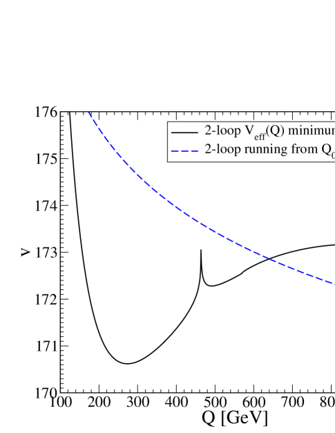
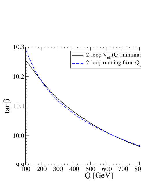
Figure 2: Comparison of the values of $v(Q)$ and $\tan\beta(Q)$ as a test of renormalization scale invariance. The solid lines are values obtained directly from minimization of the two-loop effective potential at the scale $Q$, using Lagrangian parameters run from $Q_{0}=640$ GeV. The dashed lines are the result obtained by renormalization group running of the template VEVs of eq. (6.3) from $Q_{0}$ to $Q$ using eqs. (5.8),(5.9). The discrepancy is due to effects at three loop order and beyond.

The good news is that the comparison of $v(Q)$ obtained by the two methods shows agreement to better than 0.5% for a significant range of scales $Q$ near the template scale $Q_{0}$ (which is approximately $\sqrt{m_{\tilde{t}_{1}}m_{\tilde{t}_{2}}}$), and the comparison of $\tan\beta$ is good to better than $0.1$%. However, near $Q_{0}$ the slopes of $v(Q)$ found by the two methods actually have the opposite sign! This surprising sensitivity to higher-loop effects is a consequence of the shallowness of the scalar potential along the direction $v_{u}/v_{d}\approx\tan\beta$. In contrast, higher-loop contributions have relatively much less effect on $v_{u}/v_{d}$, since that corresponds to a much steeper direction of the potential.

An aside: the cusp-like feature found near $Q=463$ GeV occurs because, at that scale, the tree-level squared mass of $h^{0}$ at the minimum of the two-loop effective potential goes through 0; it is positive for all larger $Q$. This leads to significant numerical effects because of the appearance of terms involving ln$(m_{h^{0}}^{2})$ in the effective potential:

$$V^{(1)} = {1\over 4}(m_{h^{0}}^{2})^{2}{\rm ln}(m_{h^{0}}^{2}/Q^{2})+\ldots;$$ (6.5)

$$V^{(2)} = m_{h^{0}}^{2}\left[c_{1}{\rm ln}(m_{h^{0}}^{2}/Q^{2})+c_{2}{\rm ln}^{2}(m_{h^{0}}^{2}/Q^{2})\right]+\ldots.$$ (6.6)

where $c_{1}$ and $c_{2}$ have dimensions of (mass)². Thus $V_{\rm eff}$ is well-defined in the limit $m_{h^{0}}^{2}\rightarrow 0$. However, while the first derivatives of $V^{(1)}$ with respect to $v_{u}$ and $v_{d}$ are finite, the first derivatives of $V^{(2)}$ have logarithmic and double-logarithmic divergences in that limit.

A comparison of the full two-loop effective potential to previous approximations is shown in figure 3. The graphs show the ratios $v_{\rm min}/v_{\rm run}$ and $\tan\beta_{\rm min}/\tan\beta_{\rm run}$, where “min” means obtained by direct minimization at $Q$, and “run” means obtained by running the template values of $v_{u}$, $v_{d}$ in eq. (6.3) from $Q_{0}$ to $Q$. This shows that the full two-loop effective potential indeed mitigates the scale dependence, and changes the value found for $v$ compared to the previous state-of-the-art approximation in refs. [10]-[12] by nearly $1.5$% in this example.

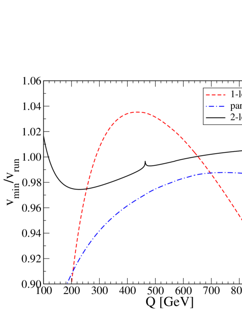
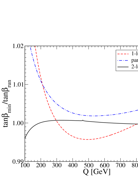
Figure 3: Comparisons of the values and scale dependence of the VEV parameters $v$ and $\tan\beta$ found by minimizing the effective potential in different approximations. The label “min” refers to values obtained by direct minimization at $Q$, and “run” means obtained by running the template values of eq. (6.3) from $Q_{0}$. The solid lines follow from the full two-loop effective potential found in section 3 of the present paper. The dashed lines represent the one-loop approximation, and the dot-dashed lines the partial two-loop approximation of refs. [10]-[12].

A different way to look at things, which may be closer to the situation we will face when confronted with experiment, is to view $v_{u}$ and $v_{d}$ as input data rather than output parameters, and use the two minimization conditions of the effective potential to extract values for two other parameters. Since $v_{u}$ and $v_{d}$ are especially sensitive to radiative corrections because of the shallowness of the potential, treating them as among the known quantities is advantageous. Here I will follow the commonplace procedure of treating $b$ and $\mu$ as the unknowns to be solved for, with given values of $v_{u}$, $v_{d}$ and all the other Lagrangian parameters. (In reality, it seems clear that global fits to various observables will have to be conducted, since no more direct measurement of $m_{H_{u}}^{2}$ and $m_{H_{d}}^{2}$ is possible.) In figure 4, I have graphed the ratios of $\mu_{\rm min}/\mu_{\rm run}$ and $b_{\rm min}/b_{\rm run}$, where “min” means that the effective potential at $Q$ is required to be minimized, using values obtained by running the Lagrangian parameters of eq. (6.1) and VEVs of eq. (6.3) from $Q_{0}$ to $Q$, while “run” means those obtained by running the template values for $\mu$, $b$ of eq. (6.2) from $Q_{0}$ to $Q$ using two-loop renormalization group equations. In each case, the full two-loop results are compared to those obtained using one-loop and partial two-loop approximations for the effective potential. In this model, the scale-dependences of $\mu$ and $b$ are less than a few hundredths of a percent, using the full two-loop potential over a wide range of scales $Q$.

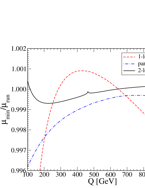
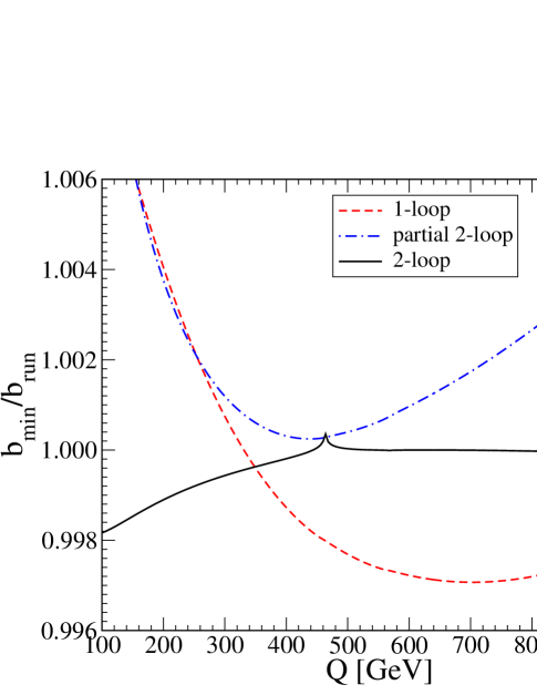
Figure 4: Comparisons of the values and scale-dependence of the parameters $\mu$ and $b$ obtained by requiring the effective potential to be minimized. The label “min” refers to values obtained by running the Lagrangian parameters of eq. (6.1) and VEVs of eq. (6.3) to $Q$, and “run” means obtained by running the template values for $\mu$, $b$ of eq. (6.2) from $Q_{0}$ to $Q$. The solid lines follow from the full two-loop effective potential found in section 3. The dashed lines represent the one-loop approximation, and the dot-dashed lines the partial two-loop approximation of refs. [10]-[12].

7 Outlook

In this paper, I have presented the complete two-loop effective potential for the MSSM in the Landau gauge and the $\overline{\rm DR}^{\prime}$ scheme.

The two-loop effective potential found here can, in principle, be renormalization-group improved [32] to sum leading and sub-leading logarithms of ratios of different mass scales. However, the logarithmic contributions to the effective potential are typically not overwhelming compared to the non-logarithmic ones. Renormalization group improvement does give an improved scale dependence, because that is what it is designed to do. However, improved scale-independence does not always imply improved accuracy; it is a necessary but not sufficient criterion. Therefore, the efficacy of further renormalization-group improvement of the MSSM effective potential on top of the full two-loop result is unclear to me.

If supersymmetry is part of the new physics associated with electroweak symmetry breaking, then these results will be part of a program to fit accurately experimental data to underlying Lagrangian parameters. Other parts of this program will require more precise calculations of the superpartner and Higgs scalar physical masses. Of particular importance is an improved calculation of the physical $h^{0}$ mass, which is well-known to be highly sensitive to radiative corrections. Unfortunately, $m_{h^{0}}^{2}$ cannot simply be obtained by taking the second derivatives of the effective potential found here, because of important wave-function renormalization effects.

The calculation described here can be extended to various non-minimal versions of supersymmetry, for example those with additional singlet fields. This can be done as a straightforward application of ref. [14] for a general theory. The fact that $h^{0}$ was not discovered at LEP may be taken as support for the importance of considering such models.

This work was supported in part by the NSF grant number PHY-9970691.

References

- [1]
- [2] S. R. Coleman and E. Weinberg, Phys. Rev. D 7, 1888 (1973).
- [3] R. Jackiw, Phys. Rev. D 9, 1686 (1974).
- [4] M. Sher, Phys. Rept. 179, 273 (1989).
- [5] H. E. Haber and G. L. Kane, Phys. Rept. 117, 75 (1985).
- [6] J. F. Gunion and H. E. Haber, Nucl. Phys. B 272, 1 (1986) [Erratum-ibid. B 402, 567 (1993)]; Nucl. Phys. B 278, 449 (1986).
- [7] S. P. Martin, “A supersymmetry primer,” [hep-ph/9709356].
- [8] S. P. Li and M. Sher, Phys. Lett. B 140, 339 (1984); Y. Okada, M. Yamaguchi and T. Yanagida, Prog. Theor. Phys. 85, 1 (1991); J. R. Ellis, G. Ridolfi and F. Zwirner, Phys. Lett. B 257, 83 (1991), Phys. Lett. B 262, 477 (1991); H. E. Haber and R. Hempfling, Phys. Rev. Lett. 66, 1815 (1991); R. Barbieri, M. Frigeni and F. Caravaglios, Phys. Lett. B 258, 167 (1991); A. Brignole, J. R. Ellis, G. Ridolfi and F. Zwirner, Phys. Lett. B 271, 123 (1991); R. Arnowitt and P. Nath, Phys. Rev. D 46, 3981 (1992); D. J. Castaño, E. J. Piard and P. Ramond, Phys. Rev. D 49, 4882 (1994); J. Kodaira, Y. Yasui and K. Sasaki, Phys. Rev. D 50, 7035 (1994) [hep-ph/9311366]; G. L. Kane, C. Kolda, L. Roszkowski and J. D. Wells, Phys. Rev. D 49, 6173 (1994) [hep-ph/9312272]; J. A. Casas, J. R. Espinosa, M. Quiros and A. Riotto, Nucl. Phys. B 436, 3 (1995) [Erratum-ibid. B 439, 466 (1995)] [hep-ph/9407389]; M. Carena, M. Quiros and C. E. Wagner, Nucl. Phys. B 461, 407 (1996) [hep-ph/9508343]. For comparisons with non-effective-potential approaches, see M. Carena, H. E. Haber, S. Heinemeyer, W. Hollik, C. E. Wagner and G. Weiglein, Nucl. Phys. B 580, 29 (2000) [hep-ph/0001002], and references therein.
- [9] R. Hempfling and A. H. Hoang, Phys. Lett. B 331, 99 (1994) [hep-ph/9401219].
- [10] R. Zhang, Phys. Lett. B 447, 89 (1999). [hep-ph/9808299].
- [11] J. R. Espinosa and R. J. Zhang, JHEP 0003, 026 (2000) [hep-ph/9912236].
- [12] J. R. Espinosa and R. Zhang, Nucl. Phys. B 586, 3 (2000). [hep-ph/0003246].
- [13] I. Jack et al., Phys. Rev. D 50, 5481 (1994). [hep-ph/9407291].
- [14] S. P. Martin, Phys. Rev. D 65, 116003 (2002) [hep-ph/0111209].
- [15] W. Siegel, Phys. Lett. B 84, 193 (1979); D. M. Capper, D.R.T. Jones and P. van Nieuwenhuizen, Nucl. Phys. B 167, 479 (1980).
- [16] A. V. Kotikov, Phys. Lett. B 254, 158 (1991); Phys. Lett. B 259, 314 (1991).
- [17] C. Ford and D.R.T. Jones, Phys. Lett. B 274, 409 (1992) [Erratum-ibid. B 285, 399 (1992)].
- [18] C. Ford, I. Jack and D.R.T. Jones, Nucl. Phys. B 387, 373 (1992) [Erratum-ibid. B 504, 551 (1992)] [hep-ph/0111190].
- [19] A. I. Davydychev and J. B. Tausk, Nucl. Phys. B 397, 123 (1993); A. I. Davydychev, V. A. Smirnov and J. B. Tausk, Nucl. Phys. B 410, 325 (1993) [hep-ph/9307371]; F. A. Berends and J. B. Tausk, Nucl. Phys. B 421, 456 (1994).
- [20] M. Caffo, H. Czyz, S. Laporta and E. Remiddi, Nuovo Cim. A 111, 365 (1998) [hep-th/9805118].
- [21] M. B. Einhorn and D.R.T. Jones, Nucl. Phys. B 211, 29 (1983).
- [22] B. Kastening, Phys. Lett. B 283, 287 (1992).
- [23] M. Bando, T. Kugo, N. Maekawa and H. Nakano, Phys. Lett. B 301, 83 (1993) [hep-ph/9210228]; Prog. Theor. Phys. 90, 405 (1993) [hep-ph/9210229].
- [24] C. Ford, D.R.T. Jones, P. W. Stephenson and M. B. Einhorn, Nucl. Phys. B 395, 17 (1993) [hep-lat/9210033].
- [25] J. R. Espinosa and I. Navarro, Nucl. Phys. B 615, 82 (2001) [hep-ph/0104047].
- [26] M. Carena, J. R. Ellis, A. Pilaftsis and C. E. Wagner, Nucl. Phys. B 625, 345 (2002).
- [27] A. Brignole, G. Degrassi, P. Slavich and F. Zwirner, Nucl. Phys. B 631, 195 (2002).
- [28] M. Frank, S. Heinemeyer, W. Hollik and G. Weiglein, [hep-ph/0202166].
- [29] D.R.T. Jones, “Supersymmetric Gauge Theories,” in TASI Lectures in elementary particle physics, Ann Arbor 1984.
- [30] Y. Yamada, Phys. Lett. B 530, 174 (2002). [hep-ph/0112251].
- [31] S. P. Martin and M. T. Vaughn, Phys. Rev. D 50, 2282 (1994). [hep-ph/9311340].
- [32] For various approaches, see refs. [21]-[24] and: H. Yamagishi, Phys. Rev. D 23, 1880 (1981), Nucl. Phys. B 216, 508 (1983); M. B. Einhorn and D.R.T. Jones, Nucl. Phys. B 230, 261 (1984); H. Nakano and Y. Yoshida, Phys. Rev. D 49, 5393 (1994) [hep-ph/9309215]; C. Ford and C. Wiesendanger, Phys. Rev. D 55, 2202 (1997) [hep-ph/9604392], Phys. Lett. B 398, 342 (1997) [hep-th/9612193]; J. A. Casas, V. Di Clemente and M. Quiros, Nucl. Phys. B 553, 511 (1999) [hep-ph/9809275]; J. M. Chung and B. K. Chung, Phys. Rev. D 60, 105001 (1999) [hep-th/9905086], J. Korean Phys. Soc. 39, 971 (2001) [hep-th/9911196]; D. V. Gioutsos, Eur. Phys. J. C 17, 675 (2000) [hep-ph/9905278].