hep-ph/0206077 DFPD-02/TH/13
hep-ph/0206077 CERN-TH/2002-127

Theoretical Models of Neutrino Masses and Mixings

Guido Altarelli 

Theory Division, CERN,

CH-1211 Genève 23, Switzerland

Ferruccio Feruglio 

Dipartimento di Fisica ‘G. Galilei’, Università di Padova and

INFN, Sezione di Padova, Via Marzolo 8, I-35131 Padua, Italy

We review theoretical ideas, problems and implications of different models for neutrino masses and mixing angles. We give a general discussion of schemes with three or more light neutrinos. Several specific examples are analyzed in some detail, particularly those that can be embedded into grand unified theories.

1 Introduction

There is by now convincing evidence, from the experimental study of atmospheric and solar neutrinos [1, 2], for the existence of at least two distinct frequencies of neutrino oscillations. This in turn implies non vanishing neutrino masses and a mixing matrix, in analogy with the quark sector and the CKM matrix. So apriori the study of masses and mixings in the lepton sector should be considered at least as important as that in the quark sector. But actually there are a number of features that make neutrinos especially interesting. In fact the smallness of neutrino masses is probably related to the fact that $\nu^{\prime}s$ are completely neutral (i.e. they carry no charge which is exactly conserved) and are Majorana particles with masses inversely proportional to the large scale where lepton number (L) conservation is violated. Majorana masses can arise from the see-saw mechanism [3], in which case there is some relation with the Dirac masses, or from higher-dimensional non-renormalisable operators which come from a different sector of the lagrangian density than any other fermion mass terms. The relation with L non conservation and the fact that the observed neutrino oscillation frequencies are well compatible with a large scale for L non-conservation, points to a tantalizing connection with Grand Unified Theories (Cut’s). So neutrino masses and mixings can represent a probe into the physics at GUT energy scales and offer a different perspective on the problem of flavour and the origin of fermion masses. There are also direct connections with important issues in astrophysics and cosmology as for example baryogenesis through leptogenesis [4] and the possibly non-negligible contribution of neutrinos to hot dark matter in the Universe.

At present there are many alternative models of neutrino masses. This variety is mostly due to the considerable experimental ambiguities that still exist. The most crucial questions to be clarified by experiment are whether the LSND signal [5] will be confirmed or will be excluded and which solar neutrino solution will eventually be established. If LSND is right we probably need at least four light neutrinos, if not we can do with only the three known ones. Which solar solution is correct fixes the corresponding mass squared difference and the associated mixing angle. Another crucial unknown is the absolute scale of neutrino masses. This is in turn related to as diverse physical questions as the possible cosmological relevance of neutrinos as hot dark matter or the rate of neutrinoless double beta decay ($0\nu\beta\beta$). If neutrinos are an important fraction of the cosmological density, say $\Omega_{\nu}\sim 0.1$, then the average neutrino mass must be considerably heavier than the splittings that are indicated by the observed atmospheric and solar oscillation frequencies. For example, for three light neutrinos, only models with almost degenerate neutrinos, with common mass $|m_{\nu}|\approx 1$ eV, are compatible with a large hot dark matter component, but in this case the existing bounds on $0\nu\beta\beta$ decay represent an important constraint. On the contrary hierarchical three neutrino models (with both signs of $\Delta m^{2}_{23}$) have the largest neutrino mass fixed by $|m|\approx\sqrt{\Delta m^{2}_{atm}}\approx 0.05$ eV. In view of all these important questions still pending it is no wonder that many different theoretical avenues are open and have been explored in the vast literature on the subject.

Here we will briefly summarize the main categories of neutrino mass models, discuss their respective advantages and difficulties and give a number of examples. We illustrate how forthcoming experiments can discriminate among the various alternatives. We will devote a special attention to the most constrained set of models, those with only three widely split neutrinos, with masses dominated by the see-saw mechanism and inversely proportional to a large mass close to the grand unification scale $M_{GUT}$. In this case one can aim at a comprehensive discussion in a GUT framework of all fermion masses. This is to some extent possible in models based on SU(5)$\times$ U(1)_F or on SO(10) (we always consider SUSY GUT’s).

2 Neutrino Masses and Lepton Number Violation

Neutrino oscillations imply neutrino masses which in turn demand either the existence of right-handed (RH) neutrinos (Dirac masses) or lepton number L violation (Majorana masses) or both. Given that neutrino masses are certainly extremely small, it is really difficult from the theory point of view to avoid the conclusion that L conservation must be violated. In fact, in terms of lepton number violation the smallness of neutrino masses can be explained as inversely proportional to the very large scale where L is violated, of order $M_{GUT}$ or even $M_{Pl}$.

Once we accept L non-conservation we gain an elegant explanation for the smallness of neutrino masses. If L is not conserved, even in the absence of heavy RH neutrinos, Majorana masses can be generated for neutrinos by dimension five operators [6] of the form

$$O_{5}=\frac{(Hl)^{T}_{i}\lambda_{ij}(Hl)_{j}}{\Lambda}+~{}h.c.~{}~{}~{},$$ (1)

with $H$ being the ordinary Higgs doublet, $l_{i}$ the SU(2) lepton doublets, $\lambda$ a matrix in flavour space and $\Lambda$ a large scale of mass, of order $M_{GUT}$ or $M_{Pl}$. Neutrino masses generated by $O_{5}$ are of the order $m_{\nu}\approx v^{2}/\Lambda$ for $\lambda_{ij}\approx{\rm O}(1)$, where $v\sim{\rm O}(100~{}{\rm GeV})$ is the vacuum expectation value of the ordinary Higgs.

We consider that the existence of RH neutrinos $\nu^{c}$ is quite plausible because all GUT groups larger than SU(5) require them. In particular the fact that $\nu^{c}$ completes the representation 16 of SO(10): 16=$\bar{5}$+10+1, so that all fermions of each family are contained in a single representation of the unifying group, is too impressive not to be significant. At least as a classification group SO(10) must be of some relevance. Thus in the following we assume that there are both $\nu^{c}$ and L non-conservation. With these assumptions the see-saw mechanism [3] is possible. Also to fix notations we recall that in its simplest form it arises as follows. Consider the SU(3) $\times$ SU(2) $\times$ U(1) invariant Lagrangian giving rise to Dirac and $\nu^{c}$ Majorana masses (for the time being we consider the $\nu$ Majorana mass terms as comparatively negligible):

$${\cal L}=-{\nu^{c}}^{T}y_{\nu}(Hl)+\frac{1}{2}{\nu^{c}}^{T}M\nu^{c}+~{}h.c.$$ (2)

The Dirac mass matrix $m_{D}\equiv y_{\nu}v/\sqrt{2}$, originating from electroweak symmetry breaking, is, in general, non-hermitian and non-symmetric, while the Majorana mass matrix $M$ is symmetric, $M=M^{T}$. We expect the eigenvalues of $M$ to be of order $M_{GUT}$ or more because $\nu^{c}$ Majorana masses are SU(3)$\times$ SU(2)$\times$ U(1) invariant, hence unprotected and naturally of the order of the cutoff of the low-energy theory. Since all $\nu^{c}$ are very heavy we can integrate them away. For this purpose we write down the equations of motion for $\nu^{c}$ in the static limit, $i.e.$ neglecting their kinetic terms:

$$-\frac{\partial{\cal L}}{\partial\nu^{c}}=y_{\nu}(Hl)-M\nu^{c}=0~{}~{}~{}.$$ (3)

From this, by solving for $\nu^{c}$, we obtain:

$$\nu^{c}=M^{-1}y_{\nu}(Hl)~{}~{}~{}.$$ (4)

We now replace in the lagrangian, eq. (2), this expression for $\nu^{c}$ and we get the operator $O_{5}$ of eq. (1) with

$$\frac{2\lambda}{\Lambda}=-y_{\nu}^{T}M^{-1}y_{\nu}~{}~{}~{}~{}~{},$$ (5)

and the resulting neutrino mass matrix reads:

$$m_{\nu}=m_{D}^{T}M^{-1}m_{D}~{}~{}~{}.$$ (6)

This is the well known see-saw mechanism result [3]: the light neutrino masses are quadratic in the Dirac masses and inversely proportional to the large Majorana mass. If some $\nu^{c}$ are massless or light they would not be integrated away but simply added to the light neutrinos. Notice that the above results hold true for any number $n$ of heavy neutral fermions $R$ coupled to the 3 known neutrinos. In this more general case $M$ is an $n$ by $n$ symmetric matrix and the coupling between heavy and light fields is described by the rectangular $n$ by 3 matrix $m_{D}$. Note that for $m_{\nu}\approx\sqrt{\Delta m^{2}_{atm}}\approx 0.05$ eV and $m_{\nu}\approx m_{D}^{2}/M$ with $m_{D}\approx v\approx 200~{}GeV$ we find $M\approx 10^{15}~{}GeV$ which indeed is an impressive indication for $M_{GUT}$.

If additional non-renormalisable contributions to $O_{5}$, eq. 1, are comparatively non-negligible, they should simply be added. After elimination of the heavy right-handed fields, at the level of the effective low-energy theory, the two types of terms are equivalent. In particular they have identical transformation properties under a chiral change of basis in flavour space. The difference is, however, that in the see-saw mechanism, the Dirac matrix $m_{D}$ is presumably related to ordinary fermion masses because they are both generated by the Higgs mechanism and both must obey GUT-induced constraints. Thus if we assume the see-saw mechanism more constraints are implied.

3 Baryogenesis via Leptogenesis from Heavy $\nu^{c}$ Decay

In the Universe we observe an apparent excess of baryons over antibaryons. It is appealing that one can explain the observed baryon asymmetry by dynamical evolution starting from an initial state of the Universe with zero baryon number (baryogenesis). For baryogenesis one needs the three famous Sakharov conditions: B violation, CP violation and no thermal equilibrium. In the history of the Universe these necessary requirements can have occurred at different epochs. Note however that the asymmetry generated by one epoch could be erased at following epochs if not protected by some dynamical reason. In principle these conditions could be verified in the SM at the electroweak phase transition. B is violated by instantons when kT is of the order of the weak scale (but B-L is conserved), CP is violated by the CKM phase and sufficiently marked out-of- equilibrium conditions could be realized during the electroweak phase transition. So the conditions for baryogenesis at the weak scale in the SM superficially appear to be present. However, a more quantitative analysis [7], shows that baryogenesis is not possible in the SM because there is not enough CP violation and the phase transition is not sufficiently strong first order, unless $m_{H}<80~{}{\rm GeV}$, which is by now completely excluded by LEP. In SUSY extensions of the SM, in particular in the MSSM, there are additional sources of CP violations and the bound on $m_{H}$ is modified by a sufficient amount by the presence of scalars with large couplings to the Higgs sector, typically the s-top. What is required is that $m_{h}\sim 80-110~{}{\rm GeV}$, a s-top not heavier than the top quark and, preferentially, a small $\tan{\beta}$. This possibility has by now become very marginal with the results of the LEP2 running.

If baryogenesis at the weak scale is excluded by the data it can occur at or just below the GUT scale, after inflation. But only that part with $|{\rm B}-{\rm L}|>0$ would survive and not be erased at the weak scale by instanton effects. Thus baryogenesis at $kT\sim 10^{10}-10^{15}~{}{\rm GeV}$ needs B-L violation at some stage like for $m_{\nu}$ if neutrinos are Majorana particles. The two effects could be related if baryogenesis arises from leptogenesis then converted into baryogenesis by instantons [4]. Recent results on neutrino masses are compatible with this elegant possibility [8]. Thus the case of baryogenesis through leptogenesis has been boosted by the recent results on neutrinos [9].

In leptogenesis the departure from equilibrium is determined by the deviation from the average number density induced by the decay of the heavy neutrinos. The Yukawa interactions of the heavy Majorana neutrinos $\nu^{c}$ lead to the decays $\nu^{c}\rightarrow lH$ (with $l$ a lepton) and $\nu^{c}\rightarrow\bar{l}\bar{H}$ with CP violation. The violation of L conservation arises from the $\Delta{\rm L}=2$ terms that produce the Majorana mass terms. The rates of the various interaction processes involved are temperature dependent with different powers of $T$, so that the equilibrium densities and the temperatures of decoupling from equilibrium during the Universe expansion are different for different particles and interactions. The rates $\Gamma_{\Delta L}(T)$ of $\Delta{\rm L}=2$ processes depend also on the neutrino masses and mixings, so that the observed values of the baryon asymmetry are related to neutrino processes. Precisely, $\Gamma_{\Delta L}(T)\sim T^{3}/\Lambda^{2}$ where $\Lambda$ is the large scale that appears in eq. (1) and also in the expression of light neutrino masses $m_{\nu}\sim v^{2}/\Lambda$. The out-of-equilibrium condition $\Gamma_{\Delta L}(T)<\Gamma_{exp}$, where $\Gamma_{exp}\sim T^{2}/M_{Pl}$ is the expansion rate of the Universe, leads to $T\mathrel{\hbox to0.0pt{\raise 2.15277pt\hbox{$<$}\hss}{\lower 2.15277pt\hbox{$\sim$}}}\Lambda^{2}/M_{Pl}$ which then implies the relation (when correct proportionality factors and sum over flavours are included):

$$\sum_{i}m_{\nu_{i}}^{2}\mathrel{\hbox to0.0pt{\raise 2.15277pt\hbox{$<$}\hss}{\lower 2.15277pt\hbox{$\sim$}}}[0.2~{}{\rm eV}(\frac{10^{12}~{}{\rm GeV}}{T})^{1/2}]^{2}$$ (7)

What exactly is the temperature $T$ which is relevant for leptogenesis depends on the thermal history of the early Universe and goes beyond the realm of neutrino physics. But if $T\mathrel{\hbox to0.0pt{\raise 2.15277pt\hbox{$<$}\hss}{\lower 2.15277pt\hbox{$\sim$}}}\Lambda^{2}/M_{Pl}$ and $\Lambda\sim M_{GUT}$ then the upper limit is significant and compatible with present neutrino data.

If the RH neutrinos are thermally produced, then the mass of the RH neutrino that drives L violation is limited by the reheat temperature after inflation, which in turn is typically required not to exceed $10^{8}-10^{10}$ GeV. This limit can be evaded if the RH neutrinos are instead produced by large inflaton oscillations during the preheating stage [10].

4 Four (or More) Neutrino Models

The LSND signal [5] has not been confirmed by KARMEN [11]. It will be soon double-checked by MiniBoone [12]. Perhaps it will fade away. But if an oscillation with $\Delta m^{2}\approx 1~{}{\rm eV}^{2}$ is confirmed then, in presence of three distinct frequencies for LSND, atmospheric [1] and solar [2] neutrino oscillations, the simplest possibility is to introduce at least four light neutrinos. Since LEP has limited to three the number of “active” neutrinos (that is with weak interactions, or equivalently with non-vanishing weak isospin, the only possible gauge charge of neutrinos) the additional light neutrino(s) $\nu_{s}$ must be “sterile”, i.e. with vanishing weak isospin. Note that $\nu^{c}$ that appears in the see-saw mechanism, if it exists, is indeed a sterile neutrino, but a heavy one.

A possibility to accommodate atmospheric, solar and LSND evidences for neutrino oscillations without introducing one or more sterile neutrinos is to invoke CPT violation [13]. The required independent frequencies are provided by different neutrino and anti-neutrino masses and the fit to the present data has a good quality [14].

A typical pattern of masses that works for 4-$\nu$ models consists of two pairs of neutrinos [15] with mass separation between the two pairs, of order $1~{}{\rm eV}$, corresponding to the LSND frequency. The upper doublet is almost degenerate at $m^{2}$ of order $1~{}{\rm eV}^{2}$ being only split by (the mass squared difference corresponding to) the atmospheric (solar) $\nu$ frequency, while the lower doublet is split by the solar (atmospheric) $\nu$ frequency. An alternative to this 2-2 spectrum is given by a 3-1 pattern with 1 being a nearly pure sterile neutrino separated by the LSND frequency from the 3. The 3-1 spectrum leads to a comparable (poor) overall quality of fit as the 2-2 pattern. These mass configurations can be compatible with an important fraction of hot dark matter in the universe. A complication is that the data appear to be incompatible with pure 2-$\nu$ oscillations for $\nu_{e}-\nu_{s}$ oscillations for solar neutrinos [16] and for $\nu_{\mu}-\nu_{s}$ oscillations for atmospheric neutrinos [17]. There are however (after SNO, marginally) viable alternatives. One possibility is obtained by using the large freedom allowed by the presence of 6 mixing angles in the most general 4-$\nu$ mixing matrix. If at least 4 angles are significantly different from zero, one can go beyond pure 2-$\nu$ oscillations and, for example, for solar neutrino oscillations $\nu_{e}$ can transform into a mixture of $\nu_{a}$ and $\nu_{s}$, where $\nu_{a}$ is an active neutrino, itself a superposition of $\nu_{\mu}$ and $\nu_{\tau}$ (mainly $\nu_{\tau}$) [15]. A different alternative is to have many interfering sterile neutrinos: this is the case in the interesting class of models with large extra dimensions, where a whole tower of Kaluza-Klein neutrinos is introduced. This picture of sterile neutrinos from extra dimensions appears exciting and we now discuss it in some detail [19].

The context is theories with large extra dimensions. Gravity propagates in all $D$ dimensions (bulk), while SM particles live on a 4d brane. As well known [20], this can make the fundamental scale of gravity $M_{D}$ much smaller than the Planck mass $M_{Pl}$. In fact for $D~{}=~{}\delta~{}+~{}4$ we have a geometrical factor $V_{\delta}$, the volume of the compact dimensions, that suppresses gravity, so that

$$(M_{D})^{\delta}~{}V_{\delta}~{}=~{}(M_{Pl}/M_{D})^{2}~{}~{}~{},$$ (8)

and, as a result, $M_{D}$ can be as small as $\sim 1~{}{\rm TeV}$. For neutrino phenomenology we need a really large extra dimension, with a radius $R$ at least of the order of the scale set by the observed solar oscillation frequencies, $1/R\mathrel{\hbox to0.0pt{\raise 2.15277pt\hbox{$<$}\hss}{\lower 2.15277pt\hbox{$\sim$}}}0.01~{}{\rm eV}$ or $R\mathrel{\hbox to0.0pt{\raise 2.15277pt\hbox{$>$}\hss}{\lower 2.15277pt\hbox{$\sim$}}}0.02~{}mm$. If we insist on having $M_{D}$ around $1~{}{\rm TeV}$ we can assume, for instance, one compact dimension with radius $R$ and $\delta-1$ dimensions with a common radius $R^{\prime}$, such that the volume $V_{\delta}=(2\pi)^{\delta}RR^{\prime\delta-1}$ fits eq. (8). In string theories of gravity there are always scalar fields associated with gravity together with their SUSY fermionic partners (dilatini, modulini) [21]. These are particles that propagate in the bulk, have no gauge interactions and can well play the role of sterile neutrinos. The models based on this framework [22, 23] have some good features that make them very appealing at first sight. They provide a “physical” picture for $\nu_{s}$. In the simplest case the theory includes a 5d fermion $\Psi(x,y)$, which decomposes into two 4d Weyl spinors $\nu_{s}(x,y)$ and $\nu_{s}^{\prime}(x,y)$ and contains a KK tower of recurrences of sterile neutrinos:

$$\nu_{s}(x,y)~{}=~{}\frac{1}{\sqrt{2\pi R}}\sum_{n}~{}\nu_{s}^{(n)}(x)e^{i\frac{ny}{R}}~{}~{}~{}.$$ (9)

The tower mixes with the ordinary light active neutrinos in the lepton doublet $l$:

$$S_{mix}=\int d^{4}x\frac{h}{\sqrt{M_{5}}}\nu_{s}(x,0)H(x)l(x)~{}~{}~{}.$$ (10)

The interaction is restricted to the 4d brane at $y=0$ where SM fields live. Since the 5d spinor $\nu_{s}(x,y)$ has mass dimension 2, we need the mass parameter $M_{5}\equiv M_{D}^{\delta}(2\pi R^{\prime})^{\delta-1}$ to keep the Yukawa coupling constant dimensionless. From eqs. (8,9,10), after electroweak symmetry breaking, we find:

$$S_{mix}=\int d^{4}x\sum_{n}\frac{hv}{\sqrt{2}}\frac{M_{D}}{M_{Pl}}\nu_{s}^{(n)}(x)\nu_{a}(x)~{}~{}~{},$$ (11)

where $\langle H\rangle\equiv v/\sqrt{2}$ and $\nu_{a}$ is the active neutrino embedded in $l$. Note that the geometrical factor $M_{D}/M_{Pl}$, which automatically suppresses the Yukawa coupling $h$, arises naturally from the fact that the sterile neutrino tower lives in the bulk. An additional mass parameter $\mu$, related to a possible bulk mass term for the 5d fermion $\Psi(x,y)$ is also allowed (in more realistic realizations, more 5d fields and L-violating interactions can be present).

The pattern of oscillations results from the superposition of infinite components with increasing frequencies $\sim n^{2}$ and decreasing amplitudes $\sim 1/n^{2}$. The leading oscillation frequency, $\sqrt{\Delta m^{2}}$, and the dominant mixing angle are determined by $\mu$ and $m=hvM_{D}/M_{Pl}$, whereas the number of KK excitations that effectively take part in the oscillation is controlled by $1/R$. Indeed, if $1/R\gg\sqrt{\Delta m^{2}}$, the KK modes, whose masses are approximately given by $n/R$, decouple, with the possible exception of the lightest mode. If on the contrary $1/R\mathrel{\hbox to0.0pt{\raise 2.15277pt\hbox{$<$}\hss}{\lower 2.15277pt\hbox{$\sim$}}}\sqrt{\Delta m^{2}}$, then several KK levels participate to the oscillation and the resulting energy dependence of the survival/conversion probability can appreciably differ from that of the two level case. Indeed the contribution of a few KK states makes the solar oscillation spectrum more compatible with the data. Note in passing that $\nu_{s}$ mixings must be small due to existing limits from weak processes, supernovae and nucleosynthesis [23], so that the preferred solution for this KK $\nu$ model is MSW SA. Instead the KK states should decouple in the case of atmospheric neutrino oscillations. These constraints fix the range of admissible values of R as specified above.

In spite of its good properties there are problems with this picture, in our opinion. The first property that we do not like of models with large extra dimensions is that the connection with GUT’s is lost. In particular the elegant explanation of the smallness of neutrino masses in terms of the large scale where the L conservation is violated in general evaporates. Since $M_{D}\sim 1~{}{\rm TeV}$ is small, what forbids on the brane an operator of the form $(Hl)^{T}_{i}\lambda_{ij}(Hl)_{j}/M_{D}$ which would lead to by far too large $\nu$ masses? One must impose by hand L conservation on the brane and that it is only broken by some Majorana masses of sterile $\nu$’s in the bulk, which we find somewhat ad hoc. Another problem is that we would expect gravity to know nothing about flavour, but here we would need RH partners for $\nu_{e}$, $\nu_{\mu}$ and $\nu_{\tau}$. Also a single large extra dimension has problems, because it implies [24] a linear evolution of the gauge couplings with energy from $0.01~{}{\rm eV}$ to $M_{D}\sim 1~{}{\rm TeV}$. But for more large extra dimensions the KK recurrences do not decouple fast enough. Perhaps a compromise at d=2 is possible. In conclusion the models with large extra dimension are interesting because they are speculative and fascinating but the more conventional framework still appears more plausible at closer inspection.

5 Three-Neutrino Models

We now assume that the LSND signal will not be confirmed, so that there are only two distinct neutrino oscillation frequencies, the atmospheric and the solar frequencies. These two can be reproduced with the known three light neutrino species (for other reviews of three neutrino models see [25, 26]).

Neutrino oscillations are due to a misalignment between the flavour basis, $\nu^{\prime}\equiv(\nu_{e},\nu_{\mu},\nu_{\tau})$, where $\nu_{e}$ is the partner of the mass and flavour eigenstate $e^{-}$ in a left-handed (LH) weak isospin SU(2) doublet (similarly for $\nu_{\mu}$ and $\nu_{\tau})$) and the mass eigenstates $\nu\equiv(\nu_{1},\nu_{2},\nu_{3})$ [27]:

$$\nu^{\prime}=U\nu~{}~{}~{},$$ (12)

where $U$ is the unitary 3 by 3 mixing matrix. Given the definition of $U$ and the transformation properties of the effective light neutrino mass matrix $m_{\nu}$:

$${\nu^{\prime}}^{T}m_{\nu}\nu^{\prime} = \nu^{T}U^{T}m_{\nu}U\nu$$ (13)

$$U^{T}m_{\nu}U = {\rm Diag}\left(m_{1},m_{2},m_{3}\right)\equiv m_{diag}~{}~{}~{},$$

we obtain the general form of $m_{\nu}$ (i.e. of the light $\nu$ mass matrix in the basis where the charged lepton mass is a diagonal matrix):

$$m_{\nu}=Um_{diag}U^{T}~{}~{}~{}.$$ (14)

The matrix $U$ can be parameterized in terms of three mixing angles $\theta_{12}$, $\theta_{23}$ and $\theta_{13}$ ($0\leq\theta_{ij}\leq\pi/2$) and one phase $\varphi$ ($0\leq\varphi\leq 2\pi$) [28], exactly as for the quark mixing matrix $V_{CKM}$. The following definition of mixing angles can be adopted:

$$U~{}=~{}\left(\matrix{1&0&0\cr 0&c_{23}&s_{23}\cr 0&-s_{23}&c_{23}}\right)\left(\matrix{c_{13}&0&s_{13}e^{i\varphi}\cr 0&1&0\cr-s_{13}e^{-i\varphi}&0&c_{13}}\right)\left(\matrix{c_{12}&s_{12}&0\cr-s_{12}&c_{12}&0\cr 0&0&1}\right)$$ (15)

where $s_{ij}\equiv\sin\theta_{ij}$, $c_{ij}\equiv\cos\theta_{ij}$. In addition we have the relative phases among the Majorana masses $m_{1}$, $m_{2}$ and $m_{3}$. If we choose $m_{3}$ real and positive, these phases are carried by $m_{1,2}\equiv|m_{1,2}|e^{i\phi_{1,2}}$. Thus, in general, 9 parameters are added to the SM when non vanishing neutrino masses are included: 3 eigenvalues, 3 mixing angles and 3 CP violating phases.

In our notation the two frequencies, $\Delta m^{2}_{I}/4E$ $(I=sun,atm)$, are parametrized in terms of the $\nu$ mass eigenvalues by

$$\Delta m^{2}_{sun}\equiv|\Delta m^{2}_{12}|,~{}~{}~{}~{}~{}~{}~{}\Delta m^{2}_{atm}\equiv|\Delta m^{2}_{23}|~{}~{}~{}.$$ (16)

where $\Delta m^{2}_{12}=|m_{2}|^{2}-|m_{1}|^{2}$ and $\Delta m^{2}_{23}=m_{3}^{2}-|m_{2}|^{2}$. The numbering 1,2,3 corresponds to our definition of the frequencies and in principle may not coincide with the ordering from the lightest to the heaviest state.

Table 1: Square mass differences and mixing angles [16, 17, 18].

	lower limit	best value	upper limit
	($3\sigma$)		($3\sigma$)
$(\Delta m^{2}_{sun})_{\rm LA}~{}(10^{-5}~{}{\rm eV}^{2})$	2.3	5	37
$(\Delta m^{2}_{sun})_{\rm LOW}~{}(10^{-8}~{}{\rm eV}^{2})$	3.5	8	12
$\Delta m^{2}_{atm}~{}(10^{-3}~{}{\rm eV}^{2})$	1	3	6
$(\tan^{2}\theta_{12})_{\rm LA}$	0.24	0.4	0.89
$(\tan^{2}\theta_{12})_{\rm LOW}$	0.43	0.6	0.86
$\tan^{2}\theta_{23}$	0.33	0.8	3.3
$\tan^{2}\theta_{13}$	0	0	0.07

From experiment, see table 1, we know that $c_{23}\sim s_{23}\sim 1/\sqrt{2}$, corresponding to nearly maximal atmospheric neutrino mixing, and that $s_{13}$ is small, according to CHOOZ, $s_{13}<0.2$ [29]. The solar angle $\theta_{12}$ is probably large (MSW LA, LOW, VO solutions) or even maximal for LOW and VO, but could, alternatively, be very small $s_{12}^{2}\sim O(10^{-3})$ [16], if the now disfavoured MSW SA solution is also kept in our list. If we take maximal $s_{23}$ and keep only linear terms in $u=s_{13}e^{i\varphi}$ from experiment we find the following structure of the $U_{fi}$ ($f=e$,$\mu$,$\tau$, $i=1,2,3$) mixing matrix, apart from sign convention redefinitions:

$$U_{fi}=\left(\matrix{c_{12}&s_{12}&u\cr-(s_{12}+c_{12}u^{*})/\sqrt{2}&(c_{12}-s_{12}u^{*})/\sqrt{2}&1/\sqrt{2}\cr(s_{12}-c_{12}u^{*})/\sqrt{2}&-(c_{12}+s_{12}u^{*})/\sqrt{2}&1/\sqrt{2}}\right)~{}~{}~{}~{}~{}.$$ (17)

Given the observed frequencies and our notation in eq. (16), there are three possible patterns of mass eigenvalues:

$${\rm{Degenerate}} : |m_{1}|\sim|m_{2}|\sim|m_{3}|\gg|m_{i}-m_{j}|$$

$${\rm{Inverted~{}hierarchy}} : |m_{1}|\sim|m_{2}|\gg|m_{3}|$$

$${\rm{Normal~{}hierarchy}} : |m_{3}|\gg|m_{2,1}|$$ (18)

In the following we will discuss the phenomenology for these different cases and the respective advantages and problems.

5.1 Degenerate Neutrinos

For degenerate neutrinos the average $m^{2}$ is much larger than the splittings. At first sight the degenerate case is the most appealing: the observation of nearly maximal atmospheric neutrino mixing and the experimental indication that also the solar mixing is large (at present the MSW SA solution of the solar neutrino oscillations appears disfavoured by the data [16]) suggests that all $\nu$ masses are nearly degenerate. Moreover, the common value of $|m_{\nu}|$ could be compatible with a large fraction of hot dark matter in the universe if $|m_{\nu}|\sim 1-2$ eV. In this case, however, the existing limits [30] on the absence of $0\nu\beta\beta$ ($|m_{ee}|<0.2$ eV or to be more conservative $|m_{ee}|<0.3-0.5$ eV) imply [31] double maximal mixing (bimixing) for solar and atmospheric neutrinos. In fact the quantity which is bound by experiments is the 11 entry of the $\nu$ mass matrix, which in general, from eqs. (13) and (15), is given by :

$$|m_{ee}|~{}=|(1-s^{2}_{13})~{}(m_{1}c^{2}_{12}~{}+~{}m_{2}s^{2}_{12})+m_{3}e^{2i\phi}s^{2}_{13}|~{}~{}~{},$$ (19)

which in this particular case ($m_{3}$ cannot compensate for the smallness of $s^{2}_{13}$) approximately becomes:

$$|m_{ee}|~{}\approx~{}|m_{1}c^{2}_{12}~{}+~{}m_{2}s^{2}_{12}|~{}\mathrel{\hbox to0.0pt{\raise 2.15277pt\hbox{$<$}\hss}{\lower 2.15277pt\hbox{$\sim$}}}~{}0.3-0.5~{}{\rm eV}~{}~{}~{}.$$ (20)

To satisfy this constraint one needs $m_{1}\approx-m_{2}$ (recall that a relative phase $\phi_{2}-\phi_{1}$ is allowed between $m_{1}$ and $m_{2}$) and $c^{2}_{12}\approx s^{2}_{12}$ to a good accuracy (in fact we need $\sin^{2}2\theta_{12}>0.96$ in order that $|\cos 2\theta_{12}|~{}=~{}|\cos^{2}\theta_{12}-\sin^{2}\theta_{12}|<0.2$). This is exemplified by the following texture

$$m_{\nu}=m\left(\begin{array}[]{ccc}0&-1/\sqrt{2}&1/\sqrt{2}\\ -1/\sqrt{2}&(1+\eta)/2&(1+\eta)/2\\ 1/\sqrt{2}&(1+\eta)/2&(1+\eta)/2\end{array}\right)~{}~{}~{},$$ (21)

where $\eta\ll 1$, corresponding to an exact bimaximal mixing, $s_{13}=0$ and the eigenvalues are $m_{1}=m$, $m_{2}=-m$ and $m_{3}=(1+\eta)m$. This texture has been proposed in the context of a spontaneously broken SO(3) flavor symmetry and it has been studied to analyze the stability of the degenerate spectrum against radiative corrections [32]. A more realistic mass matrix can be obtained by adding small perturbations to $m_{\nu}$ in eq. (21):

$$m_{\nu}=m\left(\begin{array}[]{ccc}\delta&-1/\sqrt{2}&(1-\epsilon)/\sqrt{2}\\ -1/\sqrt{2}&(1+\eta)/2&(1+\eta-\epsilon)/2\\ (1-\epsilon)/\sqrt{2}&(1+\eta-\epsilon)/2&(1+\eta-2\epsilon)/2\end{array}\right)~{}~{}~{}~{}~{}~{}({\tt D1})~{}~{}~{},$$ (22)

where $\epsilon$ parametrizes the leading flavor-dependent radiative corrections (mainly induced by the $\tau$ Yukawa coupling) and $\delta$ controls $m_{ee}$. Consider first the case $\delta\ll\epsilon$. To first approximation $\theta_{12}$ remains maximal. We get $\Delta m^{2}_{sun}\approx m^{2}\epsilon^{2}/\eta$ and

$$\theta_{13}\approx\left(\frac{\Delta m^{2}_{sun}}{\Delta m^{2}_{atm}}\right)^{{1}/{2}}~{}~{}~{},~{}~{}~{}~{}~{}~{}~{}~{}~{}m_{ee}\ll m~{}\left(\frac{\Delta m^{2}_{atm}~{}\Delta m^{2}_{sun}}{m^{4}}\right)^{1/2}~{}~{}~{}.$$ (23)

If we instead assume $\delta\gg\epsilon$, we find $\Delta m^{2}_{sun}\approx 2m^{2}\delta$, $\theta_{23}\approx\pi/4$, $\sin^{2}2\theta_{12}\approx 1-\delta^{2}/4$. Also in this case the solar mixing angle remains close to $\pi/4$. We get:

$$\theta_{13}\approx 0~{}~{}~{},~{}~{}~{}~{}~{}~{}~{}~{}~{}~{}~{}~{}~{}m_{ee}\approx\frac{\Delta m^{2}_{sun}}{2m}~{}~{}~{},$$ (24)

too small for detection if the average neutrino mass $m$ is around the eV scale. This example shows that there is no guarantee for $m_{ee}$ to be close to the range of experimental interest, even with degenerate neutrinos where the involved masses are much larger than the oscillation frequencies. However, an almost maximal solar mixing angle such as the one implied by the previous analysis, is difficult to reconcile with the MSW LA solution. Of course the strong constraint $s^{2}_{12}=c^{2}_{12}$ can be relaxed if the common mass is below the hot dark matter maximum. It is true in any case that a signal of $0\nu\beta\beta$ near the present limit (like a large relic density of hot dark matter) would be an indication for nearly degenerate $\nu$’s.

In general, for naturalness reasons, the splittings cannot be too small with respect to the common mass, unless there is a protective symmetry [32, 33]. This is because the wide mass differences of fermion masses, in particular charged lepton masses, would tend to create neutrino mass splittings via renormalization group running effects even starting from degenerate masses at a large scale. For example, for $m\approx 1$ eV, the VO solution for solar neutrino oscillations would imply $\Delta m/m\sim 10^{-9}-10^{-11}$ which is difficult to obtain. Even in the previous example, where, for $\delta\ll\epsilon$, the corrections to $\Delta m^{2}_{sun}$ are quadratic in $\epsilon$ rather than linear, we would need $\epsilon<(10^{-3}/m({\rm eV}))^{2}$ in order to have $\Delta m^{2}_{sun}<10^{-9}~{}{\rm eV}^{2}$. In this respect the MSW LA or LOW solutions would be favoured, but, if we insist that $|m_{\nu}|\sim 1-2~{}{\rm eV}$, it is not clear that the mixing angle preferred by the data is sufficiently maximal. Summarizing, degenerate models with $|m|\sim 1-2~{}{\rm eV}$ as required if $\nu$’s are a cosmologically important source of hot dark matter have some problems related to $0\nu\beta\beta$ limits and to naturalness. In comparison degenerate models with sub-eV common mass appear simpler to realize.

It is clear that in the degenerate case the most likely origin of $\nu$ masses is from some dimension 5 operators $(Hl)^{T}_{i}\lambda_{ij}(Hl)_{j}/\Lambda$ not related to the see-saw mechanism $m_{\nu}=m^{T}_{D}M^{-1}m_{D}$. In fact we expect the $\nu$ Dirac mass $m_{D}$ not to be degenerate like for all other fermions and a conspiracy to reinstate a nearly perfect degeneracy between $m_{D}$ and $M$, which arise from completely different physics, looks very unplausible (see, however, [34]). Thus in degenerate models, in general, there is no direct relation with Dirac masses of quarks and leptons and the possibility of a simultaneous description of all fermion masses within a grand unified theory is more remote [35].

The degeneracy of neutrinos should be guaranteed by some slightly broken symmetry. Models based on discrete or continuous symmetries have been proposed. For example in the models of ref. [36] the symmetry is SO(3). In the unbroken limit neutrinos are degenerate and charged leptons are massless. When the symmetry is broken the charged lepton masses are much larger than neutrino splittings because the former are first order while the latter are second order in the electroweak symmetry breaking.

A model which is simple to describe but difficult to derive in a natural way is one [37] where up quarks, down quarks and charged leptons have “democratic” mass matrices, with all entries equal (in first approximation):

$$m_{f}={\hat{m}}_{f}\left(\matrix{1&1&1\cr 1&1&1\cr 1&1&1}\right)+\delta m_{f}~{}~{}~{},$$ (25)

where ${\hat{m}}_{f}$ ($f=u,d,e$) are three overall mass parameters and $\delta m_{f}$ denote small perturbations. If we neglect $\delta m_{f}$, the eigenvalues of $m_{f}$ are given by $(0,0,3~{}{\hat{m}}_{f})$. The mass matrix $m_{f}$ is diagonalized by a unitary matrix $U_{f}$ which is in part determined by the small term $\delta m_{f}$. If $\delta m_{u}\approx\delta m_{d}$, the CKM matrix, given by $V_{CKM}=U_{u}^{\dagger}U_{d}$, is nearly diagonal, due to a compensation between the large mixings contained in $U_{u}$ and $U_{d}$. When the small terms $\delta m_{f}$ are diagonal and of the form $\delta m_{f}={\rm Diag}(-\epsilon_{f},\epsilon_{f},\delta_{f})$ the matrices $U_{f}$ are approximately given by (note the analogy with the quark model eigenvalues $\pi^{0}$, $\eta$ and $\eta^{\prime}$):

$$U_{f}^{\dagger}\approx\left(\matrix{1/\sqrt{2}&-1/\sqrt{2}&0\cr 1/\sqrt{6}&1/\sqrt{6}&-2/\sqrt{6}\cr 1/\sqrt{3}&1/\sqrt{3}&1/\sqrt{3}}\right)~{}~{}~{}.$$ (26)

At the same time, the lightest quarks and charged leptons acquire a non-vanishing mass. The leading part of the mass matrix in eq. (25) is invariant under a discrete $S_{3L}\times S_{3R}$ permutation symmetry. The same requirement leads to the general neutrino mass matrix:

$$m_{\nu}=m\left[\left(\begin{array}[]{ccc}1&0&0\\ 0&1&0\\ 0&0&1\end{array}\right)+r\left(\begin{array}[]{ccc}1&1&1\\ 1&1&1\\ 1&1&1\end{array}\right)\right]+\delta m_{\nu}~{}~{}~{}~{}~{}~{}~{}~{}~{}~{}({\tt D2})~{}~{}~{},$$ (27)

where $\delta m_{\nu}$ is a small symmetry breaking term and the two independent invariants are allowed by the Majorana nature of the light neutrinos. If $r$ vanishes the neutrinos are almost degenerate. In the presence of $\delta m_{\nu}$ the permutation symmetry is broken and the degeneracy is removed. If, for example, we choose $\delta m_{\nu}={\rm Diag}(0,\epsilon,\eta)$ with $\epsilon<\eta\ll 1$ and $r\ll\epsilon$, the solar and the atmospheric oscillation frequencies are determined by $\epsilon$ and $\eta$, respectively. The mixing angles are almost entirely due to the charged lepton sector. A diagonal $\delta m_{\rm e}$ will lead to a neutrino mixing matrix $U\approx U_{e}^{\dagger}$ characterized by an almost maximal $\theta_{12}$, $\tan^{2}\theta_{23}\approx 1/2$ and

$$\theta_{13}\approx\sqrt{m_{e}/m_{\mu}}~{}~{}~{}.$$ (28)

By going to the basis where the charged leptons are diagonal, we can see that $m_{ee}$ is close to $m$ and independent from the parameters that characterize the oscillation phenomena.

The parameter $r$ receives radiative corrections [38] that, at leading order, are logarithmic and proportional to the square of the $\tau$ lepton Yukawa coupling. It is important to guarantee that this correction does not spoil the relation $r\ll\epsilon$, whose violation would lead to a completely different mixing pattern. This raises a ‘naturalness’ problem for the LOW and VO solutions. We conclude by stressing that a non-vanishing $\Delta m^{2}_{atm}$, maximal $\theta_{12}$, large $\theta_{23}$ and vanishing $\theta_{13}$ are not determined by the symmetric limit, but only by a specific choice of the parameter $r$ and of the perturbations that cannot be easily justified on theoretical grounds. It would be desirable to provide a more sound basis for the choice of the small terms in this scenario that is quite favourable to signals both in the $0\nu 2\beta$ decay and in sub-leading oscillations controlled by $\theta_{13}$.

Anarchical models [39] can be considered as particular cases of degenerate models with $m^{2}\sim\Delta m^{2}_{atm}$. In this class of models one assumes that all mass matrices are structureless in the leptonic sector. At present the data appear to indicate the MSW LA solution as the most likely one. For this solution the ratio of the solar and atmospheric frequencies is not so small: typically ${(\Delta m^{2}_{sun})}_{LA}/\Delta m^{2}_{atm}\sim 0.01-0.2$ and two out of three mixing angles are large. One important observation is that the see-saw mechanism tends to enhance the ratio of eigenvalues: it is quadratic in $m_{D}$ so that a hierarchy factor $f$ in $m_{D}$ becomes $f^{2}$ in $m_{\nu}$ and the presence of the Majorana matrix $M$ results in a further widening of the distribution. Another squaring takes place in going from the masses to the oscillation frequencies which are quadratic. As a result a random generation of the $m_{D}$ and $M$ matrix elements leads to a distribution of ${(\Delta m^{2}_{sun})}_{LA}/\Delta m^{2}_{atm}$ that peaks around 0.1. At the same time the distribution of $\sin^{2}{\theta_{ij}}$ is peaked around 1 for all three mixing angles. Clearly the smallness of $\theta_{13}$ is problematic. This can be turned into the prediction that in anarchical models $\theta_{13}$ must be near the present bound (after all the value 0.2 for $\sin{\theta_{13}}$ is not that smaller than the maximal value 0.701). In conclusion there is a non negligible probability that if the MSW LA solution is realized and $\theta_{13}$ is near the present bound than the neutrino masses and mixings, interpreted by the see-saw mechanism, just arise from structureless underlying Dirac and Majorana matrices.

5.2 Inverted Hierarchy

The inverted hierarchy configuration $|m_{1}|\sim|m_{2}|\gg|m_{3}|$ consists of two levels $m_{1}$ and $m_{2}$ with small splitting $\Delta m_{12}^{2}~{}=~{}\Delta m_{sun}^{2}$ and a common mass given by $|m_{1,2}^{2}|\sim|\Delta m_{atm}^{2}|\sim 3\cdot 10^{-3}~{}eV^{2}$ (no large hot dark matter component in this case). One particularly interesting example of this sort [40], which leads to double maximal mixing, is obtained with the phase choice $m_{1}=-m_{2}$ so that, approximately:

$$m_{diag}~{}=~{}{\rm Diag}(\sqrt{2}m,-\sqrt{2}m,0)~{}~{}~{}.$$ (29)

The effective light neutrino mass matrix

$$m_{\nu}~{}=~{}Um_{diag}U^{T}~{}~{}~{},$$ (30)

which corresponds to the mixing matrix of double maximal mixing $c_{12}=s_{12}=1/\sqrt{2}$ and $s_{13}=u=0$ in eq. (17).

$$U_{fi}=\left(\matrix{1/\sqrt{2}&1/\sqrt{2}&0\cr-1/2&1/2&1/\sqrt{2}\cr 1/2&-1/2&1/\sqrt{2}}\right)~{}~{}~{},$$ (31)

is given by:

$$m_{\nu}~{}=~{}m\left(\matrix{0&-1&1\cr-1&0&0\cr 1&0&0}\right)~{}~{}~{}.$$ (32)

The structure of $m_{\nu}$ can be reproduced by imposing a flavour symmetry $L_{e}-L_{\mu}-L_{\tau}$ starting either from $(Hl)^{T}_{i}\lambda_{ij}(Hl)_{j}/\Lambda$ or from RH neutrinos via the see-saw mechanism. The $1-2$ degeneracy remains stable under radiative corrections. The preferred solar solutions are VO or the LOW solution. The MSW LA could be also compatible if the mixing angle is large enough.

The leading texture in (32) can be perturbed by adding small terms:

$$m_{\nu}=m\left(\begin{array}[]{ccc}\delta&-1&1\\ -1&\eta&\eta\\ 1&\eta&\eta\end{array}\right)~{}~{}~{}~{}~{}~{}~{}~{}~{}~{}({\tt I})~{}~{}~{},$$ (33)

where $\delta$ and $\eta$ are small ($\ll 1$), real parameters defined up to coefficients of order 1 that can differ in the various matrix elements. The perturbations leave $\Delta m^{2}_{atm}$ and $\theta_{23}$ unchanged, in first approximation. We obtain $\tan^{2}\theta_{12}\approx 1+\delta+\eta$ and $\Delta m^{2}_{sun}/\Delta m^{2}_{atm}\approx\eta+\delta$, where coefficients of order one have been neglected. Moreover $\theta_{13}\approx\eta$. If $\eta\gg\delta$, we have

$$\theta_{13}\approx\frac{\Delta m^{2}_{sun}}{\Delta m^{2}_{atm}}~{}~{}~{},~{}~{}~{}~{}~{}~{}~{}~{}~{}~{}~{}~{}~{}~{}m_{ee}\ll\sqrt{\Delta m^{2}_{sun}}\left(\frac{\Delta m^{2}_{sun}}{\Delta m^{2}_{atm}}\right)^{\frac{1}{2}}~{}~{}~{}.$$ (34)

In the other case, $\eta\ll\delta$ we obtain:

$$\theta_{13}\ll\frac{\Delta m^{2}_{sun}}{\Delta m^{2}_{atm}}~{}~{}~{},~{}~{}~{}~{}~{}~{}~{}~{}~{}~{}~{}~{}~{}~{}m_{ee}\approx\frac{1}{2}\sqrt{\Delta m^{2}_{sun}}\left(\frac{\Delta m^{2}_{sun}}{\Delta m^{2}_{atm}}\right)^{\frac{1}{2}}~{}~{}~{}.$$ (35)

There is a well-known difficulty of this scenario to fit the MSW LA solution [40, 41]. Indeed, barring cancellation between the perturbations, in order to obtain a $\Delta m^{2}_{sun}$ close to the best fit MSW LA value, $\eta$ and $\delta$ should be smaller than about 0.1 and this keeps the value of $\sin^{2}2\theta_{12}$ very close to 1, somewhat in disagreement with global fits of solar data [16]. Even by allowing for a $\Delta m^{2}_{sun}$ in the upper range of the MSW LA solution, or some fine-tuning between $\eta$ and $\delta$, we would need large values of the perturbations to fit the MSW LA solution. On the contrary, the LOW solution can be accommodated, but, in this case, $\theta_{13}$ and $m_{ee}$ estimated in (34,35) are too small to be detected by planned experiments.

5.3 Normal Hierarchy

We now discuss the class of models which we consider of particular interest being the most constrained framework which allows a comprehensive combined study of all fermion masses in GUT’s. We assume three widely split $\nu$’s and the existence of a RH neutrino for each generation, as required to complete a 16 dimensional representation of SO(10) for each generation. We then assume dominance of the see-saw mechanism $m_{\nu}=m_{D}^{T}M^{-1}m_{D}$. We know that the third-generation eigenvalue of the Dirac mass matrices of up and down quarks and of charged leptons is systematically the largest one. It is natural to imagine that this property could also be true for the Dirac mass of $\nu$’s: $m_{D}^{diag}\sim{\rm Diag}(0,0,m_{D3})$. After see-saw we expect $m_{\nu}$ to be even more hierarchical being quadratic in $m_{D}$ (barring fine-tuned compensations between $m_{D}$ and $M$). The amount of hierarchy, $m^{2}_{3}/m^{2}_{2}=\Delta m^{2}_{atm}/\Delta m^{2}_{sun}$, depends on which solar neutrino solution is adopted: the hierarchy is maximal for VO and LOW solutions, is moderate for MSW in general and could become quite mild for the upper $\Delta m^{2}_{sun}$ domain of the MSW LA solution. A possible difficulty is that one is used to expect that large splittings correspond to small mixings because normally only close-by states are strongly mixed. In a 2 by 2 matrix context the requirement of large splitting and large mixings leads to a condition of vanishing determinant and large off-diagonal elements. For example the matrix

$$\left(\matrix{x^{2}&x\cr x&1}\right)$$ (36)

has eigenvalues 0 and $1+x^{2}$ and for $x$ of O(1) the mixing is large. Thus in the limit of neglecting small mass terms of order $m_{1,2}$ the demands of large atmospheric neutrino mixing and dominance of $m_{3}$ translate into the condition that the 2 by 2 subdeterminant 23 of the 3 by 3 mixing matrix approximately vanishes. The problem is to show that this vanishing can be arranged in a natural way without fine tuning. Once near maximal atmospheric neutrino mixing is reproduced the solar neutrino mixing can be arranged to be either small or large without difficulty by implementing suitable relations among the small mass terms.

It is not difficult to imagine mechanisms that naturally lead to the approximate vanishing of the 23 sub-determinant. For example [42, 43] assumes that one $\nu^{c}$ is particularly light and coupled to $\mu$ and $\tau$. In a 2 by 2 simplified context if we have

$$M\propto\left(\matrix{\epsilon&0\cr 0&1}\right)~{}~{}~{},~{}~{}~{}~{}~{}~{}~{}M^{-1}\approx\left(\matrix{1/\epsilon&0\cr 0&0}\right)~{}~{}~{},~{}~{}~{}~{}~{}~{}~{}m_{D}=\left(\matrix{a&b\cr c&d}\right)~{}~{}~{},$$ (37)

then for a generic $m_{D}$ we find

$$m_{\nu}~{}=~{}m_{D}^{T}M^{-1}m_{D}\approx\frac{1}{\epsilon}\left(\matrix{a^{2}&ab\cr ab&b^{2}}\right)~{}~{}~{}.$$ (38)

A different possibility that we find attractive is that, in the limit of neglecting terms of order $m_{1,2}$ and, in the basis where charged leptons are diagonal, the Dirac matrix $m_{D}$, defined by $\nu^{c}m_{D}\nu$, takes the approximate form, called “lopsided” [44, 45, 46]:

$$m_{D}\propto\left(\matrix{0&0&0\cr 0&0&0\cr 0&x&1}\right)~{}~{}~{}~{}~{}.$$ (39)

This matrix has the property that for a generic Majorana matrix $M$ one finds:

$$m_{\nu}=m^{T}_{D}M^{-1}m_{D}\propto\left(\matrix{0&0&0\cr 0&x^{2}&x\cr 0&x&1}\right)~{}~{}~{}.$$ (40)

The only condition on $M^{-1}$ is that the 33 entry is non zero. However, when the approximately vanishing matrix elements are replaced by small terms, one must also assume that no new O(1) terms are generated in $m_{\nu}$ by a compensation between small terms in $m_{D}$ and large terms in $M^{-1}$. It is important for the following discussion to observe that $m_{D}$ given by eq. (39) under a change of basis transforms as $m_{D}\to V^{\dagger}m_{D}U$ where $V$ and $U$ rotate the right and left fields respectively. It is easy to check that in order to make $m_{D}$ diagonal we need large left mixings (i.e. large off diagonal terms in the matrix that rotates LH fields). Thus the question is how to reconcile large LH mixings in the leptonic sector with the observed near diagonal form of $V_{CKM}$, the quark mixing matrix. Strictly speaking, since $V_{CKM}=U^{\dagger}_{u}U_{d}$, the individual matrices $U_{u}$ and $U_{d}$ need not be near diagonal, but $V_{CKM}$ does, while the analogue for leptons apparently cannot be near diagonal. However for quarks nothing forbids that, in the basis where $m_{u}$ is diagonal, the $d$ quark matrix has large non diagonal terms that can be rotated away by a pure RH rotation. We suggest that this is so and that in some way RH mixings for quarks correspond to LH mixings for leptons.

In the context of (SUSY) SU(5) there is a very attractive hint of how the present mechanism can be realized [47, 48]. In the $\bar{5}$ of SU(5) the $d^{c}$ singlet appears together with the lepton doublet $(\nu,e)$. The $(u,d)$ doublet and $e^{c}$ belong to the 10 and $\nu^{c}$ to the 1 and similarly for the other families. As a consequence, in the simplest model with mass terms arising from only Higgs pentaplets, the Dirac matrix of down quarks is the transpose of the charged lepton matrix: $m_{d}=(m_{l})^{T}$. Thus, indeed, a large mixing for RH down quarks corresponds to a large LH mixing for charged leptons. At leading order we may have the lopsided texture:

$$m_{d}=(m_{l})^{T}=\left(\matrix{0&0&0\cr 0&0&1\cr 0&0&1}\right)v_{d}~{}~{}~{}.$$ (41)

In the same simplest approximation with 5 or $\bar{5}$ Higgs, the up quark mass matrix is symmetric, so that left and right mixing matrices are equal in this case. Then small mixings for up quarks and small LH mixings for down quarks are sufficient to guarantee small $V_{CKM}$ mixing angles even for large $d$ quark RH mixings. It is well known that a model where the down and the charged lepton matrices are exactly the transpose of one another cannot be exactly true because of the $e/d$ and $\mu/s$ mass ratios. It is also known that one remedy to this problem is to add some Higgs component in the 45 representation of SU(5) [49]. But the symmetry under transposition can still be a good guideline if we are only interested in the order of magnitude of the matrix entries and not in their exact values. Similarly, the Dirac neutrino mass matrix $m_{D}$ is the same as the up quark mass matrix in the very crude model where the Higgs pentaplets come from a pure 10 representation of SO(10): $m_{D}=m_{u}$. For $m_{D}$ the dominance of the third family eigenvalue as well as a near diagonal form could be an order of magnitude remnant of this broken symmetry. Thus, neglecting small terms, the neutrino Dirac matrix in the basis where charged leptons are diagonal could be directly obtained in the form of eq. (39).

To get a realistic mass matrix, we allow for deviations from the symmetric limit in (40), where we take $x=1$. For instance, we can consider those models where the neutrino mass matrix elements are dominated, via the see-saw mechanism, by the exchange of two right-handed neutrinos [43]. Since the exchange of a single RH neutrino gives a successful zeroth order texture, we are encouraged to continue along this line. Thus, we add a sub-dominant contribution of a second RH neutrino, assuming that the third one gives a negligible contribution to the neutrino mass matrix, because it has much smaller Yukawa couplings or is much heavier than the first two. The Lagrangian that describes this plausible subset of see-saw models, written in the mass eigenstate basis of RH neutrinos and charged leptons, is

$${\cal L}=y_{i}\nu^{c}Hl_{i}+y^{\prime}_{i}{\nu^{c}}^{\prime}Hl_{i}+\frac{M}{2}{\nu^{c}}^{2}+\frac{M^{\prime}}{2}{\nu^{c}}^{\prime 2}~{}~{}~{},$$ (42)

leading to

$$({m_{\nu}})_{ij}\propto\frac{y_{i}y_{j}}{M}+\frac{y^{\prime}_{i}y^{\prime}_{j}}{M^{\prime}}~{}~{}~{},$$ (43)

where $i,j=\{e,\mu,\tau\}$. In particular, if $y_{e}\ll y_{\mu}\approx y_{\tau}$ and $y^{\prime}_{\mu}\approx y^{\prime}_{\tau}$, we obtain:

$$m_{\nu}=m\left(\begin{array}[]{ccc}\delta&\epsilon&\epsilon\\ \epsilon&1+\eta&1+\eta\\ \epsilon&1+\eta&1+\eta\end{array}\right)~{}~{}~{}~{}~{}~{}~{}~{}~{}~{}({\tt N})~{}~{}~{},$$ (44)

where coefficients of order one multiplying the small quantities $\delta$, $\epsilon$ and $\eta$ have been omitted. The mass matrix in (44) does not describe the most general perturbation of the zeroth order texture (40). We have implicitly assumed a symmetry between $\nu_{\mu}$ and $\nu_{\tau}$ which is preserved by the perturbations, at least at the level of the order of magnitudes. The perturbed texture (44) can also arise when the zeroes of the lopsided Dirac matrix in (39) are replaced by small quantities. It is possible to construct models along this line based on a spontaneously broken U(1)_F flavor symmetry, where $\delta$, $\epsilon$ and $\eta$ are given by positive powers of one or more symmetry breaking parameters. Moreover, by playing with the U(1)_F charges, we can adjust, to certain extent, the relative hierarchy between $\eta$, $\epsilon$ and $\delta$ [42, 43, 45, 46, 47, 48], as we will see in section 8. The texture (44) can also be generated in SUSY models with $R$-parity violation [50].

After a first rotation by an angle $\theta_{23}$ close to $\pi/4$ and a second rotation with $\theta_{13}\approx\epsilon$, we get

$$m_{\nu}\approx m\left(\begin{array}[]{ccc}\delta+\epsilon^{2}&\epsilon&0\\ \epsilon&\eta&0\\ 0&0&2\end{array}\right)~{}~{}~{},$$ (45)

up to order one coefficients in the small entries. To obtain a large solar mixing angle, we need $|\eta-\delta|<\epsilon$. In realistic models there is no reason for a cancellation between independent perturbations and thus we assume both $\delta\leq\epsilon$ and $\eta\leq\epsilon$.

Consider first the case $\delta\approx\epsilon$ and $\eta<\epsilon$. The solar mixing angle $\theta_{12}$ is large but not maximal, as preferred by the MSW LA solution. We also have $\Delta m^{2}_{atm}\approx 4m^{2}$, $\Delta m^{2}_{sun}\approx\Delta m^{2}_{atm}\epsilon^{2}$ and

$$m_{ee}\approx\sqrt{\Delta m^{2}_{sun}}~{}~{}~{}.$$ (46)

If $\eta\approx\epsilon$ and $\delta\ll\epsilon$, we still have a large solar mixing angle and $\Delta m^{2}_{sun}\approx\epsilon^{2}\Delta m^{2}_{atm}$, as before. However $m_{ee}$ will be much smaller than the estimate in (46). Unfortunately, this is the case of the models based on the above mentioned U(1)_F flavor symmetry that, at least in its simplest realization, tends to predict $\delta\approx\epsilon^{2}$. In this class of models we find

$$m_{ee}\approx\sqrt{\Delta m^{2}_{sun}}\left(\frac{\Delta m^{2}_{sun}}{\Delta m^{2}_{atm}}\right)^{\frac{1}{2}}~{}~{}~{},$$ (47)

below the sensitivity of the next generation of planned experiments. It is worth to mention that in both cases discussed above, we have

$$\theta_{13}\approx\left(\frac{\Delta m^{2}_{sun}}{\Delta m^{2}_{atm}}\right)^{\frac{1}{2}}~{}~{}~{},$$ (48)

which might be very close to the present experimental limit.

If both $\delta$ and $\eta$ are much smaller than $\epsilon$, the 12 block of $m_{\nu}$ has an approximate pseudo-Dirac structure and the angle $\theta_{12}$ becomes maximal. This situation is typical of some models where leptons have U(1)_F charges of both signs whereas the order parameters of U(1)_F breaking have all charges of the same sign [47]. We have two eigenvalues approximately given by $\pm m~{}\epsilon$. As an example, we consider the case where $\eta=0$ and $\delta\approx\epsilon^{2}$. We find $\sin^{2}2\theta_{12}\approx 1-\epsilon^{2}/4$, $\Delta m^{2}_{sun}\approx m^{2}\epsilon^{3}$ and

$$\theta_{13}\approx\left(\frac{\Delta m^{2}_{sun}}{\Delta m^{2}_{atm}}\right)^{\frac{1}{3}}~{}~{}~{},~{}~{}~{}~{}~{}~{}~{}~{}~{}~{}~{}m_{ee}\approx\sqrt{\Delta m^{2}_{sun}}\left(\frac{\Delta m^{2}_{sun}}{\Delta m^{2}_{atm}}\right)^{\frac{1}{6}}~{}~{}~{}.$$ (49)

In order to recover the MSW LA solution we would need a relatively large value of $\epsilon$. This is in general not acceptable because, on the one hand the presence of a large perturbation raises doubts about the consistency of the whole approach and, on the other hand, in existing models where all fermion sectors are related to each other, $\epsilon$ is never larger than the Cabibbo angle. Therefore, the case $\delta,\eta\ll\epsilon$ can be more easily adapted to fit the LOW solution where the solar frequency is small. As a consequence, $m_{ee}$ is beyond the reach of the next generation of experiments, whereas $\theta_{13}$ might be tested at future facilities.

5.4 Summary

Given the present experimental knowledge, which favours $\Delta m^{2}_{atm}$ as the leading oscillation frequency and two large mixing angles, $\theta_{23}$ and $\theta_{12}$, it is natural to define a zeroth order approximation of the theory, where $\Delta m^{2}_{sun}$ and $\theta_{13}$ vanish (which allows us to neglect the CP-breaking parameter $\varphi$) whereas $\theta_{23}$ and $\theta_{12}$ are maximal. For each pattern of neutrino masses, we have considered the most interesting textures that arise in this limit.

Table 2: Order-of-magnitude estimates for $\theta_{13}$.

Texture	$\theta_{12}$	$\theta_{13}$	Perturbations
		$\approx\left(\frac{\Delta m^{2}_{sun}}{\Delta m^{2}_{atm}}\right)^{1/2}$	$\epsilon\gg\delta$
$m_{\nu}^{\rm D1}=m\left(\begin{array}[]{ccc}\delta&-\frac{1}{\sqrt{2}}&\frac{(1-\epsilon)}{\sqrt{2}}\\ -\frac{1}{\sqrt{2}}&\frac{(1+\eta)}{2}&\frac{(1+\eta-\epsilon)}{2}\\ \frac{(1-\epsilon)}{\sqrt{2}}&\frac{(1+\eta-\epsilon)}{2}&\frac{(1+\eta-2\epsilon)}{2}\end{array}\right)$	$\approx\pi/4$
		$\approx 0$	$\epsilon\ll\delta$
$m_{\nu}^{\rm D2}=m\left[\left(\begin{array}[]{ccc}1&0&0\\ 0&1&0\\ 0&0&1\end{array}\right)+r\left(\begin{array}[]{ccc}1&1&1\\ 1&1&1\\ 1&1&1\end{array}\right)\right]+\delta m_{\nu}$	$\approx\pi/4$	$\approx\left(\frac{m_{e}}{m_{\mu}}\right)^{1/2}$
		$\approx\frac{\Delta m^{2}_{sun}}{\Delta m^{2}_{atm}}$	$\eta\gg\delta$
$m_{\nu}^{\rm I}=m\left(\begin{array}[]{ccc}\delta&-1&1\\ -1&\eta&\eta\\ 1&\eta&\eta\end{array}\right)$	$\approx\pi/4$
		$\ll\frac{\Delta m^{2}_{sun}}{\Delta m^{2}_{atm}}$	$\eta\ll\delta$
			$\eta<\delta\approx\epsilon$
	$O(1)$	$\approx\left(\frac{\Delta m^{2}_{sun}}{\Delta m^{2}_{atm}}\right)^{1/2}$
$m_{\nu}^{\rm N}=m\left(\begin{array}[]{ccc}\delta&\epsilon&\epsilon\\ \epsilon&1+\eta&1+\eta\\ \epsilon&1+\eta&1+\eta\end{array}\right)$			$\delta\approx\epsilon^{2}\approx\eta^{2}$
	$\approx\pi/4$	$\approx\left(\frac{\Delta m^{2}_{sun}}{\Delta m^{2}_{atm}}\right)^{1/3}$	$\delta\approx\epsilon^{2}~{}~{}~{}\eta=0$

This approximation is of course not realistic and should be regarded only as a limiting case, possibly arising from an underlying symmetry. Many effects can perturb this limit, such as small symmetry breaking terms, radiative corrections, effects coming from residual rotations needed to diagonalize the charged lepton mass matrix, or to render canonical the leptonic kinetic terms. Some of these will be discussed more in detail in the next sections. It turns out that in most of the existing models the leading textures are modified by small perturbations having a simple structure, such as those called D1, D2, I and N in eqs. (22), (27), (33) and (44).

We have analyzed these perturbations, with the hope that the results are sufficiently representative of the many existing models. Of course there is no guarantee that this discussion can cover all theoretical possibilities. Moreover, if $\Delta m^{2}_{sun}$ and $\theta_{13}$ were as large as experimentally allowed, the perturbations would become large, the whole approach could become questionable and the data would be more appropriately described by an anarchical framework.

A remarkable feature is that most models continue to predict an almost maximal solar angle, even after inclusion of the perturbations. This is often due to an approximate pseudo-Dirac structure in the 12 sector, which, at leading order, forces $\theta_{12}=\pi/4$. Exceptions to this trend are given by some of the possibilities offered by the normal hierarchy, for which $\theta_{12}$ is undetermined at leading order.

It is also apparent that, apart from the case of degenerate spectrum realized with a texture similar to the one of flavor democracy (D2), the possibility of measuring $m_{ee}$ with the next generation of experiments seems to be significant only if the solar oscillation frequency is very close to the upper part of the range allowed by the MSW LA solution.

6 Importance of Neutrinoless Double Beta Decay

The discovery of $0\nu\beta\beta$ decay would be very important because it would establish lepton number violation and the Majorana nature of $\nu$’s. Indeed oscillation experiments cannot distinguish between pure Dirac and Majorana neutrinos. Moreover, the search for $0\nu\beta\beta$ decay provides information about the absolute spectrum, while neutrino oscillations are only sensitive to mass differences. Complementary information on the sum of neutrino masses is also provided by the galaxy power spectrum combined with measurements of the cosmic microwave background anisotropies [51]. As already mentioned the present limit from $0\nu\beta\beta$ is $|m_{ee}|<0.2$ eV or to be more conservative $|m_{ee}|<0.3-0.5$ eV [30]. In this respect it is interesting to see what is the level at which a signal can be expected or at least not excluded in the different classes of models [52, 53]. For 3-neutrino models with degenerate, inverse hierarchy or normal hierarchy mass patterns, starting from the general formula in eq. (19), it is simple to derive the following bounds.

• Degenerate case. If $|m|$ is the common mass, apart from a phase, and taking $s_{13}=0$, which, as already observed, is a safe approximation in this case, we have $m_{ee}=|m|(c_{12}^{2}\pm s_{12}^{2})$. Here the phase ambiguity has been reduced to a sign ambiguity which is sufficient for deriving bounds. So, depending on the sign we have $m_{ee}=|m|$ or $m_{ee}=|m|cos2\theta_{12}$. We conclude that in this case $m_{ee}$ could be very close to the present experimental limit because $|m|$ can be sizeably larger than the $0\nu\beta\beta$ bound ($|m|<O(1{\rm eV})$), but should be at least of order $O(\sqrt{\Delta m^{2}_{atm}})~{}\sim~{}O(10^{-2}~{}{\rm eV})$ unless the solar angle is practically maximal, in which case the minus sign option can be as small as required.

• Inverse hierarchy case. In this case the same approximate formula $m_{ee}=|m|(c_{12}^{2}\pm s_{12}^{2})$ holds because $m_{3}$ is small and $s_{13}$ can be neglected. The difference is that here we know that $|m|\approx\sqrt{\Delta m^{2}_{atm}}$ so that $|m_{ee}|<\sqrt{\Delta m^{2}_{atm}}~{}\sim~{}0.05$ eV.

• Normal hierarchy case. Here we cannot in general neglect the $m_{3}$ term. However in this case $|m_{ee}|~{}\sim~{}\sqrt{\Delta m^{2}_{sun}}~{}s_{12}^{2}~{}+~{}\sqrt{\Delta m^{2}_{atm}}~{}s_{13}^{2}$ and we have the bound $|m_{ee}|<$ a few $10^{-3}$ eV.

Recently evidence for $0\nu\beta\beta$ was claimed in ref. [54] at the 2-3$\sigma$ level with $|m_{ee}|\sim~{}0.39~{}{\rm eV}$. If confirmed this would rule out cases b) and c) and point to case a) or to models with more than 3 neutrinos.

7 Expectations for $\theta_{13}$

The measurement of $\theta_{13}$ represents one of the main challenges for the next generations of experiments on neutrino oscillations, which, with the help of very intense neutrino beams [55], might reach a sensitivity of few percent on $\theta_{13}$. A sizeable $\theta_{13}$ would have an important impact on the observability of CP-violating effects in the leptonic sector. We collect in table 2 our estimates of $\theta_{13}$ for the various textures considered in section 5.

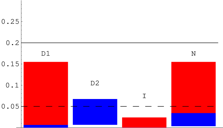
Figure 1: Order-of-magnitude estimates of $\theta_{13}$, for MSW LA solution (red) and LOW solution (blu). There is no difference between MSW LA and LOW for the texture D2. The upper limits have been obtained by using the approximate expression of table 1 and the values: $\Delta m^{2}_{atm}=2.5\cdot 10^{-3}~{}eV^{2}$, $\Delta m^{2}_{sun}=6.0\cdot 10^{-5}~{}eV^{2}~{}(10^{-7}~{}eV^{2})$ for MSW LA (LOW). The continuous and dashed lines show the present upper bound on $\theta_{13}$ and the possible reach of long baseline experiments with high intensity neutrino beams.

Figure 1 displays the expectations for $\theta_{13}$. Such expectations are of course very rough and are not meant to be statistically meaningful. It is however interesting to note that the MSW LA solution favours $\theta_{13}$ in an experimentally accessible range, for all textures but for the inverted hierarchy, where we find a strong suppression. The LOW solution prefers a smaller, unobservable $\theta_{13}$, with the possible exception of the texture D2, corresponding to flavour democracy. We recall that if the neutrino mass matrix is structureless as advocated by the anarchical framework, then $\theta_{13}$ is naturally expected to be very close to its present experimental bound.

8 Grand Unified Models of Fermion Masses

We have seen that the smallness of neutrino masses interpreted via the see-saw mechanism directly leads to a scale $\Lambda$ for L non-conservation which is remarkably close to $M_{GUT}$. Thus neutrino masses and mixings should find a natural context in a GUT treatment of all fermion masses. The hierarchical pattern of quark and lepton masses, within a generation and across generations, requires some dynamical suppression mechanism that acts differently on the various particles. This hierarchy can be generated by a number of operators of different dimensions suppressed by inverse powers of the cut-off $\Lambda_{c}$ of the theory. In some realizations, the different powers of $1/\Lambda_{c}$ correspond to different orders in some symmetry breaking parameter $v_{f}$ arising from the spontaneous breaking of a flavour symmetry. In the next subsections we describe some simplest models based on SU(5) $\times$ U(1)_F and on SO(10) which illustrate these possibilities.

8.1 Models Based on Horizontal Abelian Charges

We discuss here some explicit examples of grand unified models in the framework of a unified SUSY SU(5) theory with an additional U(1)_F flavour symmetry. The SU(5) generators act “vertically” inside one generation, while the U(1)_F charges are different “horizontally” from one generation to the other. If, for a given interaction vertex, the U(1)_F charges do not add to zero, the vertex is forbidden in the symmetric limit. But the symmetry is spontaneously broken by the VEV’s $v_{f}$ of a number of “flavon” fields with non vanishing charge. Then a forbidden coupling is rescued but is suppressed by powers of the small parameters $v_{f}/\Lambda_{c}$ with the exponents larger for larger charge mismatch [56]. We expect $v_{f}\mathrel{\hbox to0.0pt{\raise 2.15277pt\hbox{$>$}\hss}{\lower 2.15277pt\hbox{$\sim$}}}M_{GUT}$ and $\Lambda_{c}\mathrel{\hbox to0.0pt{\raise 2.15277pt\hbox{$<$}\hss}{\lower 2.15277pt\hbox{$\sim$}}}M_{Pl}$. Here we discuss some aspects of the description of fermion masses in this framework.

In these models the known generations of quarks and leptons are contained in triplets $\Psi^{10}_{i}$ and $\Psi^{\bar{5}}_{i}$, $(i=1,2,3)$ corresponding to the 3 generations, transforming as $10$ and ${\bar{5}}$ of SU(5), respectively. Three more SU(5) singlets $\Psi^{1}_{i}$ describe the RH neutrinos. In SUSY models we have two Higgs multiplets, which transform as 5 and $\bar{5}$ in the minimal model. The two Higgs multiplets may have the same or different charges. We can arrange the unit of charge in such a way that the Cabibbo angle, which we consider as the typical hierarchy parameter of fermion masses and mixings, is obtained when the suppression exponent is unity. Remember that the Cabibbo angle is not too small, $\lambda\sim 0.22$ and that in U(1)_F models all mass matrix elements are of the form of a power of a suppression factor times a number of order unity, so that only their order of suppression is defined. As a consequence, in practice, we can limit ourselves to integral charges in our units (for example, $\sqrt{\lambda}\sim 1/2$ is already almost unsuppressed).

There are many variants of these models: fermion charges can all be non negative with only negatively charged flavons, or there can be fermion charges of different signs with either flavons of both charges or only flavons of one charge. We can have that only the top quark mass is allowed in the symmetric limit, or that also other third generation fermion masses are allowed. The Higgs charges can be equal, in particular both vanishing or can be different. We can arrange that all the structure is in charged fermion masses while neutrinos are anarchical.

8.1.1 F(fermions)$\geq$ 0

Consider, for example, a simple model with all charges of matter fields being non negative and containing one single flavon ${\bar{\theta}}$ of charge F$=-1$. For a maximum of simplicity we also assume that all the third generation masses are directly allowed in the symmetric limit. This is realized by taking vanishing charges for the Higgses and for the third generation components $\Psi^{10}_{3}$, $\Psi^{\bar{5}}_{3}$ and $\Psi^{1}_{3}$. For example, if we define F$(\Psi^{R}_{i})\equiv q^{R}_{i}$ $(R=10,{\bar{5}},1;~{}i=1,2,3)$ we could take [58, 45, 46, 47] (see also [57])

$$(q^{10}_{1},q^{10}_{2},q^{10}_{3}) = (3,2,0)$$

$$(q^{\bar{5}}_{1},q^{\bar{5}}_{2},q^{\bar{5}}_{3}) = (2,0,0)~{}~{}~{}.$$ (50)

A generic mass matrix has the form

$$m~{}=~{}\left(\matrix{y_{11}\lambda^{q_{1}+q^{\prime}_{1}}&y_{12}\lambda^{q_{1}+q^{\prime}_{2}}&y_{13}\lambda^{q_{1}+q^{\prime}_{3}}\cr y_{21}\lambda^{q_{2}+q^{\prime}_{1}}&y_{22}\lambda^{q_{2}+q^{\prime}_{2}}&y_{23}\lambda^{q_{2}+q^{\prime}_{3}}\cr y_{31}\lambda^{q_{3}+q^{\prime}_{1}}&y_{32}\lambda^{q_{3}+q^{\prime}_{2}}&y_{33}\lambda^{q_{3}+q^{\prime}_{3}}}\right)v~{}~{}~{},$$ (51)

where all the $y_{ij}$ are of order 1 and $(q_{i},q^{\prime}_{j})$ are the charges of $(\Psi^{10},\Psi^{10})$ for $m_{u}$, of $(\Psi^{\bar{5}},\Psi^{10})$ for $m_{d}$ or $m^{T}_{l}$, of $(\Psi^{1},\Psi^{\bar{5}})$ for $m_{D}$ (the Dirac $\nu$ mass), and of $(\Psi^{1},\Psi^{1})$ for $M$, the Majorana $\nu^{c}$ mass, respectively. We have $\lambda\equiv\langle{\bar{\theta}}\rangle/\Lambda_{c}$ and the quantity $v$ represents the appropriate VEV or mass parameter. It is important to observe that $m$ can be written as:

$$m~{}=~{}\lambda_{R}y\lambda_{R^{\prime}}v~{}~{}~{},$$ (52)

where $\lambda_{R}={\rm Diag}(\lambda^{q_{1}^{R}},\lambda^{q_{2}^{R}},\lambda^{q_{3}^{R}})$ and $y$ is the $y_{ij}$ matrix. The models with all non negative charges and one single flavon have particularly simple factorization properties. For example, if we start from the Dirac $\nu$ matrix: $m_{D}~{}=~{}\lambda_{1}y_{D}\lambda_{\bar{5}}v_{u}$ and the $\nu^{c}$ Majorana matrix $M~{}=~{}\lambda_{1}y_{M}\lambda_{1}\Lambda$ and write down the see-saw expression for $m_{\nu}=m_{D}^{T}M^{-1}m_{D}$, we find that the dependence on the $q^{1}$ charges drops out and only that from $q^{\bar{5}}$ remains. As a consequence the effective light neutrino Majorana mass matrix $m_{\nu}$ can be written in terms of $q^{\bar{5}}$ only: $m_{\nu}=\lambda_{\bar{5}}(y_{D}^{T}y_{M}^{-1}y_{D})\lambda_{\bar{5}}\cdot v_{u}^{2}/\Lambda$. In addition, for the neutrino mixing matrix $U_{ij}$, which is determined by $m_{\nu}$ in the basis where the charged leptons are diagonal, one can prove that $U_{ij}\approx\lambda^{|q^{\bar{5}}_{i}-q^{\bar{5}}_{j}|}$, in terms of the differences of the $\bar{5}$ charges, when terms that are down by powers of the small parameter $\lambda$ are neglected. Similarly the CKM matrix elements are approximately determined by only the 10 charges [56]: $V^{CKM}_{ij}\approx\lambda^{|q^{10}_{i}-q^{10}_{j}|}$. With these results in mind, we understand that the $q^{10}$ charge assignments in eq. (50) are determined by requiring $V_{us}\sim\lambda$, $V_{cb}\sim\lambda^{2}$ and $V_{ub}\sim\lambda^{3}$. However the same $q^{10}$ charges also fix $m_{u}:m_{c}:m_{t}\sim\lambda^{6}:\lambda^{4}:1$. The experimental value of $m_{u}$ (the relevant mass values are those at the GUT scale: $m=m(M_{GUT})$ [59]) would rather prefer $q^{10}_{1}=4$. Taking into account this indication and the presence of the unknown coefficients $y_{ij}\sim O(1)$ it is difficult to decide between $q^{10}_{1}=3$ or $4$ and both are acceptable.

Turning to the $\bar{5}$ charges, the entries $q^{\bar{5}}_{2}=q^{\bar{5}}_{3}=0$ have been selected in eq. (50) so that the 22, 23, 32, 33 entries of the effective light neutrino mass matrix $m_{\nu}$ are all O(1) in order to accommodate the nearly maximal value of $s_{23}$. The small non diagonal terms of the charged lepton mass matrix cannot change this. In fact, for $q^{10}_{i}$, $q^{\bar{5}}_{i}$ chosen as in eqs. (50) we obtain:

$$m_{d}=\left(\matrix{\lambda^{5}&\lambda^{4}&\lambda^{2}\cr\lambda^{3}&\lambda^{2}&1\cr\lambda^{3}&\lambda^{2}&1}\right)v_{d}~{}~{}=(m_{l})^{T}~{},~{}~{}~{}~{}m_{\nu}=\left(\matrix{\lambda^{4}&\lambda^{2}&\lambda^{2}\cr\lambda^{2}&1&1\cr\lambda^{2}&1&1}\right){v_{u}^{2}\over\Lambda}~{}~{}~{},$$ (53)

where $v_{u,d}$ are the VEVs of the Higgs doublets. Note that the patterns $m_{d}:m_{s}:m_{b}\sim m_{e}:m_{\mu}:m_{\tau}\sim\lambda^{5}:\lambda^{2}:1$ are acceptable (but also $q^{5}_{1}=3$ would be possible). One difficulty is that for $m_{\nu}$ the subdeterminant 23 is not suppressed in this case, so that the splitting between the 2 and 3 light neutrino masses is in general small. In spite of the fact that $m_{D}$ is, in first approximation, of the form in eq. (39) the strong correlations between $m_{D}$ and $M$ implied by the simple charge structure of the model destroy the vanishing of the 23 subdeterminant that would be guaranteed for generic $M$. Models of this sort have been proposed in the literature [58, 45]. The hierarchy between $m_{2}$ and $m_{3}$ is considered accidental and better be moderate. The preferred solar solution in this case is MSW SA because if $m_{1}$ is suppressed (and some suppression is needed if we want $s_{13}$ small) the solar mixing angle is typically small. However, if with a moderate fine tuning we stretch by hand $m_{2}$ to become sufficiently close to $m_{1}$ then the MSW LA solution could also be reproduced. From eq. (53), taking $v_{u}\sim 250~{}{\rm GeV}$, the mass scale ${\Lambda}$ of the heavy Majorana neutrinos turns out to be close to the unification scale, ${\Lambda}\sim 10^{15}~{}{\rm GeV}$.

A different interesting possibility [60] is to recover an anarchical picture of neutrinos by taking $(q^{10}_{1},q^{10}_{2},q^{10}_{3})=(4,2,0)$ and $(q^{\bar{5},1}_{1},q^{\bar{5},1}_{2},q^{\bar{5},1}_{3})=(0,0,0)$. The 10 charges lead to an acceptable pattern for the $m_{u}$ matrix and $V_{CKM}$, as already discussed. For down quarks and charged leptons we obtain a weakened hierarchy, essentially the square root than that of up quarks: $m_{d}:m_{s}:m_{b}\sim m_{e}:m_{\mu}:m_{\tau}\sim\lambda^{4}:\lambda^{2}:1$. Finally in the neutrino sector the anarchical model is realized (both $m_{D}$ and $M$ are structureless).

Note that in all previous cases we could add a constant to $q^{\bar{5}}_{i}$, for example by taking $(q^{\bar{5}}_{1},q^{\bar{5}}_{2},q^{\bar{5}}_{3})=(4,2,2)$. This would only have the consequence to leave the top quark as the only unsuppressed mass and to decrease the resulting value of $\tan{\beta}=v_{u}/v_{d}$ down to $\lambda^{2}m_{t}/m_{b}$. A constant shift of the charges $q^{1}_{i}$ might also provide a suppression of the leading $\nu^{c}$ mass eigenvalue, from $\Lambda_{c}$ down to the appropriate scale $\Lambda$. One can also consider models where the 5 and $\bar{5}$ Higgs charges are different, as in the “realistic” SU(5) model of ref. [61]. Also in these models the top mass could be the only one to be non vanishing in the symmetric limit and the value of $\tan{\beta}$ can be adjusted.

8.1.2 F(fermions) and F(flavons) of both signs

Models with naturally large 23 splittings are obtained if we allow negative charges and, at the same time, either introduce flavons of opposite charges or stipulate that matrix elements with overall negative charge are put to zero. For example, we can assign to the fermion fields the set of F charges given by:

$$(q^{10}_{1},q^{10}_{2},q^{10}_{3}) = (3,2,0)$$

$$(q^{\bar{5}}_{1},q^{\bar{5}}_{2},q^{\bar{5}}_{3}) = (b,0,0)~{}~{}~{}~{}~{}~{}~{}~{}~{}~{}~{}~{}b\geq 2a>0$$

$$(q^{1}_{1},q^{1}_{2},q^{1}_{3}) = (a,-a,0)~{}~{}~{}.$$ (54)

We consider the Yukawa coupling allowed by U(1)_F-neutral Higgs multiplets in the $5$ and ${\bar{5}}$ SU(5) representations and by a pair $\theta$ and ${\bar{\theta}}$ of SU(5) singlets with F$=1$ and F$=-1$, respectively. If $b=2$ or 3, the up, down and charged lepton sectors are not essentially different than in the previous case. Also in this case the O(1) off-diagonal entry of $m_{l}$, typical of lopsided models, gives rise to a large LH mixing in the 23 block which corresponds to a large RH mixing in the $d$ mass matrix. In the neutrino sector, the Dirac and Majorana mass matrices are given by:

$$m_{D}=\left(\matrix{\lambda^{a+b}&\lambda^{a}&\lambda^{a}\cr\lambda^{b-a}&{\lambda^{\prime}}^{a}&{\lambda^{\prime}}^{a}\cr\lambda^{b}&1&1}\right)v_{u}~{}~{},~{}~{}~{}~{}~{}~{}M=\left(\matrix{\lambda^{2a}&1&\lambda^{a}\cr 1&{\lambda^{\prime}}^{2a}&{\lambda^{\prime}}^{a}\cr\lambda^{a}&{\lambda^{\prime}}^{a}&1}\right){\Lambda}~{}~{}~{},$$ (55)

where $\lambda^{\prime}$ is given by $\langle\theta\rangle/\Lambda_{c}$ and ${\Lambda}$ as before denotes the large mass scale associated to the RH neutrinos: ${\Lambda}\gg v_{u,d}$. After diagonalization of the charged lepton sector and after integrating out the heavy RH neutrinos we obtain the following neutrino mass matrix in the low-energy effective theory:

$$m_{\nu}=\left(\matrix{\lambda^{2b}&\lambda^{b}&\lambda^{b}\cr\lambda^{b}&1+\lambda^{a}{\lambda^{\prime}}^{a}&1+\lambda^{a}{\lambda^{\prime}}^{a}\cr\lambda^{b}&1+\lambda^{a}{\lambda^{\prime}}^{a}&1+\lambda^{a}{\lambda^{\prime}}^{a}}\right){v_{u}^{2}\over{\Lambda}}~{}~{}~{}.$$ (56)

The O(1) elements in the 23 block are produced by combining the large LH mixing induced by the charged lepton sector and the large LH mixing in $m_{D}$. A crucial property of $m_{\nu}$ is that, as a result of the see-saw mechanism and of the specific U(1)_F charge assignment, the determinant of the 23 block is automatically of $O(\lambda^{a}{\lambda^{\prime}}^{a})$ (for this the presence of negative charge values, leading to the presence of both $\lambda$ and $\lambda^{\prime}$ is essential [46, 47]). The neutrino mass matrix of eq. (56) is a particular case of the more general pattern presented in eq. (44), for $\delta\approx\lambda^{2b}$, $\epsilon\approx\lambda^{b}$ and $\eta\approx\lambda^{a}{\lambda^{\prime}}^{a}$. If we take $\lambda\approx\lambda^{\prime}$, it is easy to verify that the eigenvalues of $m_{\nu}$ satisfy the relations:

$$m_{1}:m_{2}:m_{3}=\lambda^{2(b-a)}:\lambda^{2a}:1~{}~{}.$$ (57)

The atmospheric neutrino oscillations require $m_{3}^{2}\sim 10^{-3}~{}{\rm eV}^{2}$. The squared mass difference between the lightest states is of $O(\lambda^{4a})~{}m_{3}^{2}$, not far from the MSW solution to the solar neutrino problem if we choose $a=1$. In general $U_{e3}$ is non-vanishing, of $O(\lambda^{b})$. Finally, beyond the large mixing in the 23 sector, $m_{\nu}$ provides a mixing angle $\theta_{12}\sim\lambda^{b-2a}$ in the 12 sector. For $b>2a$, we recover a small solar mixing angle. For instance, taking $b=3$ and $a=1$, $\theta_{12}$ becomes close to the range preferred by the MSW SA solution. When $b=2a$, as for instance in the case $b=2$ and $a=1$, the MSW LA solution can be reproduced.

8.1.3 F(fermions) of both signs and F(flavons) $<$0

A general problem common to all models dealing with flavour is that of recovering the correct vacuum structure by minimizing the effective potential of the theory. It may be noticed that the presence of two multiplets $\theta$ and ${\bar{\theta}}$ with opposite F charges could hardly be reconciled, without adding extra structure to the model, with a large common VEV for these fields, due to possible analytic terms of the kind $(\theta{\bar{\theta}})^{n}$ in the superpotential. We find therefore instructive to explore the consequences of allowing only the negatively charged ${\bar{\theta}}$ field in the theory.

It can be immediately recognized that, while the quark mass matrices previously discussed are unchanged, in the neutrino sector the Dirac and Majorana matrices are obtained from eq. (55) by setting $\lambda^{\prime}=0$:

$$m_{D}=\left(\matrix{\lambda^{a+b}&\lambda^{a}&\lambda^{a}\cr\lambda^{b-a}&0&0\cr\lambda^{b}&1&1}\right)v_{u}~{}~{},~{}~{}~{}~{}~{}~{}~{}~{}M=\left(\matrix{\lambda^{2a}&1&\lambda^{a}\cr 1&0&0\cr\lambda^{a}&0&1}\right){\Lambda}~{}~{}.$$ (58)

The zeros are due to the analytic property of the superpotential that makes impossible to form the corresponding F invariant by using ${\bar{\theta}}$ alone. These zeros should not be taken literally, as they will be eventually filled by small terms coming, for instance, from the diagonalization of the charged lepton mass matrix and from the transformation that put the kinetic terms into canonical form. It is however interesting to work out, in first approximation, the case of exactly zero entries in $m_{D}$ and $M$, when forbidden by F. The neutrino mass matrix obtained via see-saw from $m_{D}$ and $M$ has the same pattern as the one displayed in eq. (56). A closer inspection reveals that the determinant of the 23 block is identically zero, independently from $\lambda$. This leads to the following pattern of masses:

$$m_{1}:m_{2}:m_{3}=\lambda^{b}:\lambda^{b}:1~{}~{},~{}~{}~{}~{}~{}m_{1}^{2}-m_{2}^{2}={\rm O}(\lambda^{3b})~{}~{}.$$ (59)

Moreover the mixing in the 12 sector is almost maximal:

$$\theta_{12}={\pi\over 4}+{\rm O}(\lambda^{b})~{}~{}.$$ (60)

For $b=3$ and $\lambda\sim 0.2$, both the squared mass difference $(m_{1}^{2}-m_{2}^{2})/m_{3}^{2}$ and $\sin^{2}2\theta_{12}$ are remarkably close to the values required by the VO solution to the solar neutrino problem. This property remains reasonably stable against the perturbations induced by small terms (of order $\lambda^{5}$) replacing the zeros, coming from the diagonalization of the charged lepton sector and by the transformations that render the kinetic terms canonical. By choosing $b=2$ we obtain the LOW solution. We find quite interesting that also the just-so and the LOW solutions, requiring an intriguingly small mass difference and a bimaximal mixing, can be described, at least at the level of order of magnitudes, in the context of a “minimal” model of flavour compatible with supersymmetric SU(5). In this case the role played by supersymmetry is essential, a non-supersymmetric model with ${\bar{\theta}}$ alone not being distinguishable from the version with both $\theta$ and ${\bar{\theta}}$, as far as low-energy flavour properties are concerned.

In conclusion, models based on SU(5) $\times$ U(1)_F are clearly toy models that can only aim at a semiquantitative description of fermion masses. In fact only the order of magnitude of each matrix entry can be specified. However it is rather impressive that a reasonable description of fermion masses, now also including neutrino masses and mixings, can be obtained in this simple context, which is suggestive of a deeper relation between gauge and flavour quantum numbers. There are 12 mass eigenvalues and 6 mixing angles that are specified, modulo coefficients of order 1, in terms of a bunch of integer numbers (from half a dozen to a dozen), the charges, plus 1 or more scale parameters. In the neutrino sector we have seen that the scheme is flexible enough to accommodate all the solutions that are still possible. Models aiming at a realistic unification of electroweak and strong interactions should of course address other important questions such as the doublet-triplet splitting and its stability against quantum corrections, a proton lifetime compatible with the existing limits, a correct gauge coupling constant unification and the consistency with present bounds on flavour violation [62]. Encompassing all these features in a consistent and possibly simple model is a formidable task, that might require to go beyond the conventional formulation in terms of a four-dimensional quantum field theory.

8.2 GUT Models based on SO(10)

Models based on SO(10) times a flavour symmetry are more difficult to construct because a whole generation is contained in the 16, so that, for example for U(1)_F, one would have the same value of the charge for all quarks and leptons of each generation, which is too rigid. But the mechanism discussed so far, based on asymmetric mass matrices, can be embedded in an SO(10) grand-unified theory in a rather economic way [26, 44, 63]. The 33 entries of the fermion mass matrices can be obtained through the coupling ${\bf 16}_{3}{\bf 16}_{3}{\bf 10}_{H}$ among the fermions in the third generation, ${\bf 16}_{3}$, and a Higgs tenplet ${\bf 10}_{H}$. The two independent VEVs of the tenplet $v_{u}$ and $v_{d}$ give mass, respectively, to $t/\nu_{\tau}$ and $b/\tau$. The key point to obtain an asymmetric texture is the introduction of an operator of the kind ${\bf 16}_{2}{\bf 16}_{H}{\bf 16}_{3}{\bf 16}_{H}^{\prime}$ . This operator is thought to arise by integrating out an heavy 10 that couples both to ${\bf 16}_{2}{\bf 16}_{H}$ and to ${\bf 16}_{3}{\bf 16}_{H}^{\prime}$. If the ${\bf 16}_{H}$ develops a VEV breaking SO(10) down to SU(5) at a large scale, then, in terms of SU(5) representations, we get an effective coupling of the kind ${\bf\bar{5}}_{2}{\bf 10}_{3}{\bf\bar{5}}_{H}$, with a coefficient that can be of order one. This coupling contributes to the 23 entry of the down quark mass matrix and to the 32 entry of the charged lepton mass matrix, realizing the desired asymmetry. To distinguish the lepton and quark sectors one can further introduce an operator of the form ${\bf 16}_{i}{\bf 16}_{j}{\bf 10}_{H}{\bf 45}_{H}$, $(i,j=2,3)$, with the VEV of the ${\bf 45}_{H}$ pointing in the $B-L$ direction. Additional operators, still of the type ${\bf 16}_{i}{\bf 16}_{j}{\bf 16}_{H}{\bf 16}_{H}^{\prime}$ can contribute to the matrix elements of the first generation. The mass matrices look like:

$$m_{u}=\left(\matrix{0&0&0\cr 0&0&\epsilon/3\cr 0&-\epsilon/3&1}\right)v_{u}~{}~{},~{}~{}~{}~{}~{}~{}~{}m_{d}=\left(\matrix{0&\delta&\delta^{\prime}\cr\delta&0&\sigma+\epsilon/3\cr\delta^{\prime}&-\epsilon/3&1}\right)v_{d}~{}~{},$$ (61)

$$m_{D}=\left(\matrix{0&0&0\cr 0&0&-\epsilon\cr 0&\epsilon&1}\right)v_{u}~{}~{},~{}~{}~{}~{}~{}~{}~{}m_{l}=\left(\matrix{0&\delta&\delta^{\prime}\cr\delta&0&-\epsilon\cr\delta^{\prime}&\sigma+\epsilon&1}\right)v_{d}~{}~{}.$$ (62)

They provide a good fit of the available data in the quarks and the charged lepton sector in terms of 5 parameters (one of which is complex). In the neutrino sector one obtains a large $\theta_{23}$ mixing angle, $\sin^{2}2\theta_{12}\sim 6.6\cdot 10^{-3}$ eV² and $\theta_{13}$ of the same order of $\theta_{12}$. Mass squared differences are sensitive to the details of the Majorana mass matrix.

Looking at models with three light neutrinos only, i.e. no sterile neutrinos, from a more general point of view, we stress that in the above models the atmospheric neutrino mixing is considered large, in the sense of being of order one in some zeroth order approximation. In other words it corresponds to off-diagonal matrix elements of the same order of the diagonal ones, although the mixing is not exactly maximal. The idea that all fermion mixings are small and induced by the observed smallness of the non diagonal $V_{CKM}$ matrix elements is then abandoned. An alternative is to argue that perhaps what appears to be large is not that large after all. The typical small parameter that appears in the mass matrices is $\lambda\sim\sqrt{m_{d}/m_{s}}\sim\sqrt{m_{\mu}/m_{\tau}}\sim 0.20-0.25$. This small parameter is not so small that it cannot become large due to some peculiar accidental enhancement: either a coefficient of order 3, or an exponent of the mass ratio which is less than $1/2$ (due for example to a suitable charge assignment), or the addition in phase of an angle from the diagonalization of charged leptons and an angle from neutrino mixing. One may like this strategy of producing a large mixing by stretching small ones if, for example, he/she likes symmetric mass matrices, as from left-right symmetry at the GUT scale. In left-right symmetric models smallness of left mixings implies that also right-handed mixings are small, so that all mixings tend to be small. Clearly this set of models [65] tend to favour moderate hierarchies and a single maximal mixing, so that the MSW SA solution of solar neutrinos is preferred.

9 Conclusion

By now there are rather convincing experimental indications for neutrino oscillations. The direct implication of these findings is that neutrino masses are not all vanishing. As a consequence, the phenomenology of neutrino masses and mixings is brought to the forefront. This is a very interesting subject in many respects. It is a window on the physics of GUTs in that the extreme smallness of neutrino masses can only be explained in a natural way if lepton number conservation is violated. If so, neutrino masses are inversely proportional to the large scale where lepton number is violated. Also, the pattern of neutrino masses and mixings interpreted in a GUT framework can provide new clues on the long standing problem of understanding the origin of the hierarchical structure of quark and lepton mass matrices. Neutrino oscillations only determine differences of $m_{i}^{2}$ values and the actual scale of neutrino masses remain to be experimentally fixed. In particular, the scale of neutrino masses is important for cosmology as neutrinos are candidates for hot dark matter: nearly degenerate neutrinos with a common mass around 1- 2 eV would significantly contribute to $\Omega_{m}$, the matter density in the universe in units of the critical density. The detection of $0\nu\beta\beta$ decay would be extremely important for the determination of the overall scale of neutrino masses, the confirmation of their Majorana nature and the experimental clarification of the ordering of levels in the associated spectrum. The recent indication of a signal for $0\nu\beta\beta$ with $m_{ee}$ in a range around 0.4 eV, if confirmed, would point to a small but possibly non negligible contribution of neutrinos to $\Omega_{m}$ and, among models with 3 neutrinos, would favour those with a degenerate spectrum. The decay of heavy right-handed neutrinos with lepton number non-conservation can provide a viable and attractive model of baryogenesis through leptogenesis. The measured oscillation frequencies and mixings are remarkably consistent with this attractive possibility.

While the existence of oscillations appears to be on a ground of increasing solidity, many important experimental challenges remain. For atmospheric neutrino oscillations the completion of the K2K experiment, now stopped by the accident that has seriously damaged the Superkamiokande detector, is important for a terrestrial confirmation of the effect and for an independent measurement of the associated parameters. In the near future the experimental study of atmospheric neutrinos will continue with long baseline measurements by MINOS, OPERA, ICARUS. For solar neutrinos it is not yet clear which of the solutions, MSW SA, MSW LA, LOW and VO, is true, although a preference for the MSW LA solution appears to be indicated by the present data. This issue will be presumably clarified in the near future by the continuation of SNO and the forthcoming data from KAMLAND and Borexino. Finally a clarification by MINIBOONE of the issue of the LSND alleged signal is necessary, in order to know if 3 light neutrinos are sufficient or additional sterile neutrinos must be introduced, in spite of the apparent lack of independent evidence in the data for such sterile neutrinos and of the fact that attempts of constructing plausible and natural theoretical models have not led so far to compelling results. Further in the future there are projects for neutrino factories and/or superbeams aimed at precision measurements of the oscillation parameters and possibly the detection of CP violation effects in the neutrino sector.

Pending the solution of the existing experimental ambiguities a large variety of theoretical models of neutrino masses and mixings are still conceivable. Among 3-neutrino models we have described a variety of possibilities based on degenerate, inverted hierarchy and normal hierarchy type of spectra. Most models prefer one or the other of the possible experimental alternatives which are still open. It is interesting that the MSW LA solar oscillation solution, which at present appears somewhat favoured by the data, is perhaps the most constraining for theoretical models. For example, it is difficult to reproduce this solution in the inverted hierarchy models. The MSW LA solution can be obtained in the degenerate case, also including the anarchical scenario, and in the normal hierarchy case, but also in these cases rather special conditions must be met. In many cases the MSW LA solution corresponds to values of $\theta_{13}$ rather large, not far from the present bound. The values of $m_{ee}$ (which determines the rate of $0\nu\beta\beta$) that is found in models leading to the MSW LA solution are typically of order $\sqrt{\Delta m^{2}_{sun}}$ in the normal hierarchy case and can be even larger in the degenerate case, where the expected values are at least of order $\sqrt{\Delta m^{2}_{atm}}$ (assuming that indeed for the MSW LA solution $s_{12}$ is large but not close to maximal).

The fact that some neutrino mixing angles are large and even nearly maximal, while surprising at the start, was eventually found to be well compatible with a unified picture of quark and lepton masses within GUTs. The symmetry group at $M_{GUT}$ could be either (SUSY) SU(5) or SO(10) or a larger group. For example, we have presented a class of natural models where large right-handed mixings for quarks are transformed into large left-handed mixings for leptons by the transposition relation $m_{d}=m_{e}^{T}$ which is approximately realized in SU(5) models. In particular, we argued in favour of models with 3 widely split neutrinos. Reconciling large splittings with large mixing(s) requires some natural mechanism to implement a vanishing determinant condition. This can be obtained in the see-saw mechanism, for example, if one light right-handed neutrino is dominant, or a suitable texture of the Dirac matrix is imposed by an underlying symmetry. We have shown that these mechanisms can be naturally implemented by simple assignments of U(1)_F horizontal charges that lead to a successful semiquantitative unified description of all quark and lepton masses in SUSY SU(5)$\times$ U(1)_F. Alternative realizations based on the SO(10) unification group have also been discussed.

In conclusion, the discovery of neutrino oscillations with frequencies that point to very small $\nu$ masses has opened a window on the physics beyond the Standard Model at very large energy scales. The study of the neutrino mass and mixing matrices, which is still at the beginning, can lead to particularly exciting insights on the theory at large energies possibly as large as $M_{GUT}$.

References

- [1] The SuperKamiokande collaboration, Phys. Rev. Lett. 85, 3999 (2000); T. Toshito, for the SK collaboration, hep-ex/0105023; The MACRO collaboration, Phys. Lett. B517, 59 (2001); G. Giacomelli and M. Giorgini, for the MACRO collaboration, hep-ex/0110021.
- [2] The results of the Homestake experiment are reported in B.T. Cleveland et al., Astrophys. J. 496, 505 (1998); The Gallex collaboration, Phys. Lett. B447, 127 (1999); The SAGE collaboration, Phys. Rev. C60, 055801 (1999); The SuperKamiokande collaboration, hep-ex/0103032 and hep-ex/0103033; The GNO collaboration, Phys. Lett. B490, 16 (2000); The SNO collaboration, Phys. Rev. Lett. 87, 71301 (2001); Q. R. Ahmad et al. [SNO Collaboration], nucl-ex/0204008 and nucl-ex/0204009.
- [3] T. Yanagida, in Proc. of the Workshop on Unified Theory and Baryon Number in the Universe, KEK, March 1979; M. Gell-Mann, P. Ramond and R. Slansky, in Supergravity, Stony Brook, Sept 1979.
- [4] M. Fukugita and T. Yanagida, Phys. Lett. B 174 45 (1986).
- [5] The LSND collaboration, hep-ex/0104049.
- [6] S. Weinberg, Phys. Rev. Lett. 43, 1566 (1979).
- [7] For a review see for example: M. Trodden, Rev. Mod. Phys. 71, 1463 (1999).
- [8] K. Kainulainen and K. A. Olive in “Neutrino Mass”, Springer Tracts in Modern Physics, ed. by G. Altarelli and K. Winter.
- [9] M. A. Luty, Phys. Rev. D 45, 455 (1992); H. Murayama and T. Yanagida, Phys. Lett. B 322, 349 (1994); M. Flanz, E. A. Paschos and U. Sarkar, Phys. Lett. B 345, 248 (1995) [Erratum-ibid. B 382, 447 (1995)]; M. Plumacher, Z. Phys. C 74, 549 (1997); L. Covi, E. Roulet and F. Vissani, Phys. Lett. B 384, 169 (1996); E. Ma and U. Sarkar, Phys. Rev. Lett. 80, 5716 (1998); A. Pilaftsis, Int. J. Mod. Phys. A 14, 1811 (1999); A. Riotto and M. Trodden, Ann. Rev. Nucl. Part. Sci. 49, 35 (1999); J. R. Ellis, S. Lola and D. V. Nanopoulos, Phys. Lett. B 452, 87 (1999); W. Buchmuller and M. Plumacher, Int. J. Mod. Phys. A 15, 5047 (2000); D. Falcone and F. Tramontano, Phys. Lett. B 506, 1 (2001); H. B. Nielsen and Y. Takanishi, Phys. Lett. B 507, 241 (2001); A. S. Joshipura, E. A. Paschos and W. Rodejohann, JHEP 0108, 029 (2001); B. Brahmachari, E. Ma and U. Sarkar, Phys. Lett. B 520, 152 (2001); M. Hirsch and S. F. King, Phys. Rev. D 64, 113005 (2001); F. Buccella, D. Falcone and F. Tramontano, Phys. Lett. B 524, 241 (2002); W. Buchmuller and D. Wyler, Phys. Lett. B 521, 291 (2001); M. S. Berger and K. Siyeon, Phys. Rev. D 65, 053019 (2002); G. C. Branco, R. Gonzalez Felipe, F. R. Joaquim and M. N. Rebelo, hep-ph/0202030; M. Fujii, K. Hamaguchi and T. Yanagida, hep-ph/0202210; S. Davidson and A. Ibarra, hep-ph/0202239; E. A. Paschos, hep-ph/0204137; W. Buchmuller, hep-ph/0204288.
- [10] G. F. Giudice, M. Peloso, A. Riotto and I. Tkachev, JHEP 9908, 014 (1999); J. Garcia-Bellido and E. Ruiz Morales, Phys. Lett. B 536, 193 (2002).
- [11] The Karmen collaboration, Nucl. Phys. Proc. Suppl. 91, 191 (2000).
- [12] P. Spentzouris, Nucl. Phys. Proc. Suppl. 100, 163 (2001).
- [13] H. Murayama and T. Yanagida, Phys. Lett. B 520, 263 (2001); G. Barenboim, L. Borissov, J. Lykken and A. Y. Smirnov, hep-ph/0108199; A. d. Gouvea, hep-ph/0204077.
- [14] A. Strumia, hep-ph/0201134.
- [15] G. L. Fogli, E. Lisi and A. Marrone, Phys. Rev. D 63, 053008 (2001); O. L. Peres and A. Y. Smirnov, Nucl. Phys. B 599, 3 (2001); C. Giunti, Nucl. Phys. Proc. Suppl. 100, 244 (2001); W. Grimus and T. Schwetz, Eur. Phys. J. C 20, 1 (2001); M. C. Gonzalez-Garcia, M. Maltoni and C. Pena-Garay, hep-ph/0108073; M. Maltoni, T. Schwetz and J. W. Valle, hep-ph/0112103; A. Strumia, hep-ph/0201134.
- [16] G. L. Fogli, E. Lisi, D. Montanino and A. Palazzo, Phys. Rev. D 64, 093007 (2001); J. N. Bahcall, M. C. Gonzalez-Garcia and C. Pena-Garay, JHEP 0108, 014 (2001); hep-ph/0111150; V. Barger, D. Marfatia, K. Whisnant and B. P. Wood, hep-ph/0204253; A. Bandyopadhyay, S. Choubey, S. Goswami and D. P. Roy, hep-ph/0204286; J. N. Bahcall, M. C. Gonzalez-Garcia and C. Pena-Garay, hep-ph/0204314; P. Aliani, V. Antonelli, R. Ferrari, M. Picariello and E. Torrente-Lujan, hep-ph/0205053.
- [17] G. L. Fogli, E. Lisi and A. Marrone, Phys. Rev. D 64, 093005 (2001); M. C. Gonzalez-Garcia, M. Maltoni and C. Pena-Garay, hep-ph/0108073. M. C. Gonzalez-Garcia and Y. Nir, hep-ph/0202058.
- [18] G. Fogli and E. Lisi in “Neutrino Mass”, Springer Tracts in Modern Physics, ed. by G. Altarelli and K. Winter.
- [19] K. R. Dienes, E. Dudas and T. Gherghetta, Nucl. Phys. B 557, 25 (1999); N. Arkani-Hamed, S. Dimopoulos, G. R. Dvali and J. March-Russell, Phys. Rev. D 65, 024032 (2002);
- [20] N. Arkani-Hamed, S. Dimopoulos and G. R. Dvali, Phys. Lett. B 429, 263 (1998);
- [21] K. Benakli and A. Y. Smirnov, Phys. Rev. Lett. 79, 4314 (1997).
- [22] A. E. Faraggi and M. Pospelov, Phys. Lett. B 458, 237 (1999); G. R. Dvali and A. Y. Smirnov, Nucl. Phys. B 563, 63 (1999); R. N. Mohapatra and A. Perez-Lorenzana, Nucl. Phys. B 576, 466 (2000); Y. Grossman and M. Neubert, Phys. Lett. B 474, 361 (2000); D. O. Caldwell, R. N. Mohapatra and S. J. Yellin, Phys. Rev. D 64, 073001 (2001); A. S. Dighe and A. S. Joshipura, Phys. Rev. D 64, 073012 (2001); A. De Gouvea, G. F. Giudice, A. Strumia and K. Tobe, Nucl. Phys. B 623, 395 (2002); H. Davoudiasl, P. Langacker and M. Perelstein, hep-ph/0201128.
- [23] R. Barbieri, P. Creminelli and A. Strumia, Nucl. Phys. B 585, 28 (2000); A. Lukas, P. Ramond, A. Romanino and G. G. Ross, Phys. Lett. B 495, 136 (2000); JHEP 0104, 010 (2001).
- [24] See, for example, I. Antoniadis and K. Benakli, Int. J. Mod. Phys. A 15, 4237 (2000).
- [25] G. Altarelli and F. Feruglio, Phys. Rep. 320, 295 (1999).
- [26] S. M. Barr and I. Dorsner, Nucl. Phys. B 585, 79 (2000); I. Masina, Int. J. Mod. Phys. A 16, 5101 (2001).
- [27] B. Pontecorvo, Sov. Phys. JETP 6, 429 (1957) [Zh. Eksp. Teor. Fiz. 33, 549 (1957)]; Z. Maki, M. Nakagawa and S. Sakata, Prog. Theor. Phys. 28 (1962) 870; B. Pontecorvo, Sov. Phys. JETP 26, 984 (1968) [Zh. Eksp. Teor. Fiz. 53, 1717 (1968)]; V. N. Gribov and B. Pontecorvo, Phys. Lett. B 28, 493 (1969).
- [28] N. Cabibbo, Phys. Lett. B 72, 333 (1978).
- [29] The Chooz collaboration Phys. Lett. B466, 415 (1999); see also: The Palo Verde collaboration Phys. Rev. Lett. , 84, 3764 (2000).
- [30] The Heidelberg–Moscow collaboration, H.V. Klapdor-Kleingrothaus et al. Eur. Phys. J., A12, 147 (2001); C. E. Aalseth et al. [16EX Collaboration], hep-ex/0202026.
- [31] F. Vissani, hep-ph/9708483; H. Georgi and S. L. Glashow, Phys. Rev. D 61, 097301 (2000);
- [32] R. Barbieri, G. G. Ross and A. Strumia, JHEP 9910, 020 (1999).
- [33] J.R. Ellis, S. Lola, Phys. Lett. B458, 310 (1999); N. Haba, Y. Matsui, N. Okamura, M. Sugiura, Eur. Phys. J. C10, 677 (1999); J.A. Casas, J.R. Espinosa, A. Ibarra, I. Navarro, Nucl. Phys. B569, 82 (2000); JHEP 9909, 015 (1999); Nucl. Phys. B573, 652 (2000); N. Haba, N. Okamura, Eur. Phys. J. C14, 347 (2000); P.H. Chankowski, W. Krolikowski, S. Pokorski, Phys. Lett. B473, 109 (2000); T. K. Kuo, J. Pantaleone and G. H. Wu, Phys. Lett. B 518, 101 (2001); P. H. Chankowski and S. Pokorski, Int. J. Mod. Phys. A 17, 575 (2002); S. Antusch, J. Kersten, M. Lindner and M. Ratz, arXiv:hep-ph/0203233.
- [34] M. Jezabek, hep-ph/0205234.
- [35] Examples of degenerate models are described in A. Ioannisian, J. W. F. Valle, Phys. Lett. B332 (1994) 93; R. N. Mohapatra and S. Nussinov, Phys. Rev. D 60, 013002 (1999); Phys. Lett. B 441, 299 (1998); G. C. Branco, M. N. Rebelo and J. I. Silva-Marcos, Phys. Rev. D 62, 073004 (2000); C. Wetterich, Phys. Lett. B 451, 397 (1999); G. Perez, JHEP 0012, 027 (2000).
- [36] R. Barbieri, L. J. Hall, G. L. Kane and G. G. Ross, hep-ph/9901228.
- [37] H. Fritzsch, Z.Z. Xing, Phys. Lett. B372, 265 (1996); H. Fritzsch, Z.Z. Xing, Phys. Lett. B440, 313 (1998); H. Fritzsch, Z.Z. Xing, Prog. Part. Nucl. Phys. 45, 1 (2000); M. Fukugita, M. Tanimoto, T. Yanagida, Phys. Rev. D57 (1998) 4429; Phys. Rev. D59, 113016 (1999); M. Tanimoto, T. Watari, T. Yanagida Phys. Lett. B461, 345 (1999); S. K. Kang and C. S. Kim, Phys. Rev. D 59, 091302 (1999); M. Tanimoto, Phys. Lett. B 483, 417 (2000); E. K. Akhmedov, G. C. Branco, F. R. Joaquim and J. I. Silva-Marcos, Phys. Lett. B 498, 237 (2001). For models based on discrete symmetries see also: P. F. Harrison, D. H. Perkins and W. G. Scott, Phys. Lett. B 530, 167 (2002); P. F. Harrison and W. G. Scott, hep-ph/0203209. E. K. Akhmedov, G. C. Branco, F. R. Joaquim and J. I. Silva-Marcos, Phys. Lett. B 498, 237 (2001) [arXiv:hep-ph/0008010].
- [38] N. Haba, Y. Matsui, N. Okamura, T. Suzuki, Phys. Lett. B489, 184 (2000).
- [39] L. J. Hall, H. Murayama and N. Weiner, Phys. Rev. Lett. 84, 2572 (2000); N. Haba and H. Murayama, Phys. Rev. D 63, 053010 (2001); M. S. Berger and K. Siyeon, Phys. Rev. D 63, 057302 (2001); F. Vissani, Phys. Lett. B 508, 79 (2001).
- [40] R. Barbieri, L. J. Hall, D. R. Smith, A. Strumia and N. Weiner, JHEP 9812, 017 (1998); R. Barbieri, L. J. Hall and A. Strumia, Phys. Lett. B 445, 407 (1999); See also: Ya. B. Zeldovich, Dok. Akad. Nauk. CCCP 86, 505 (1952); E.J. Konopinsky, H. Mahmound Phys. Rev. 92, 1045 (1953); A. Zee, Phys. Lett. B93, 389 (1980); S. Petcov, Phys. Lett. B100, 245 (1982); A. S. Joshipura and S. D. Rindani, Eur. Phys. J. C 14, 85 (2000); R. N. Mohapatra, A. Perez-Lorenzana and C. A. de Sousa Pires, Phys. Lett. B 474, 355 (2000); Q. Shafi and Z. Tavartkiladze, Phys. Lett. B 482, 145 (2000); hep-ph/0101350; L. Lavoura, Phys. Rev. D 62, 093011 (2000); S. F. King and N. N. Singh, Nucl. Phys. B 596, 81 (2001); J. F. Oliver and A. Santamaria, Phys. Rev. D 65, 033003 (2002); K. S. Babu and R. N. Mohapatra, hep-ph/0201176.
- [41] I. Dorsner and S. M. Barr, Nucl. Phys. B617, 493 (2001).
- [42] S. F. King, Phys. Lett. B439 (1998) 350; Nucl. Phys. B 562, 57 (1999); S. Davidson and S. F. King, Phys. Lett. B445 (1998) 191; Q. Shafi and Z. Tavartkiladze, Phys. Lett B451(1999)129.
- [43] S. F. King, Nucl. Phys. B 576, 85 (2000).
- [44] C. H. Albright and S. M. Barr, Phys. Rev. D 58, 013002 (1998); C. H. Albright, K. S. Babu and S. M. Barr, Phys. Rev. Lett. 81, 1167 (1998); P. H. Frampton and A. Rasin, Phys. Lett. B 478, 424 (2000).
- [45] N. Irges, S. Lavignac and P. Ramond, Phys. Rev. D 58, 035003 (1998);
- [46] G. Altarelli and F. Feruglio, Phys. Lett. B 439, 112 (1998); G. Altarelli and F. Feruglio, JHEP 9811, 021 (1998).
- [47] G. Altarelli and F. Feruglio, Phys. Lett. B 451, 388 (1999).
- [48] J. Sato and T. Yanagida, Phys. Lett. B 430, 127 (1998); J. K. Elwood, N. Irges and P. Ramond, Phys. Rev. Lett. 81, 5064 (1998); Z. Berezhiani and A. Rossi, JHEP 9903, 002 (1999); K. Hagiwara and N. Okamura, Nucl. Phys. B 548, 60 (1999); M. Bando and T. Kugo, Prog. Theor. Phys. 101, 1313 (1999);
- [49] H. Georgi and C. Jarlskog, Phys. Lett. B 86, 297 (1979).
- [50] M. Drees, S. Pakvasa, X. Tata and T. ter Veldhuis, Phys. Rev. D 57, 5335 (1998); E. J. Chun, S. K. Kang, C. W. Kim and U. W. Lee, Nucl. Phys. B 544, 89 (1999); B. Mukhopadhyaya, S. Roy and F. Vissani, Phys. Lett. B 443, 191 (1998); O. C. Kong, Mod. Phys. Lett. A 14, 903 (1999); M. Bisset, O. C. Kong, C. Macesanu and L. H. Orr, Phys. Rev. D 62, 035001 (2000); A. S. Joshipura and S. K. Vempati, Phys. Rev. D 60, 111303 (1999); A. Datta, B. Mukhopadhyaya and S. Roy, Phys. Rev. D 61, 055006 (2000); B. Mukhopadhyaya, Pramana 54, 147 (2000); G. Bhattacharyya, H. V. Klapdor-Kleingrothaus and H. Pas, Phys. Lett. B 463, 77 (1999); J. C. Romao, M. A. Diaz, M. Hirsch, W. Porod and J. W. Valle, Phys. Rev. D 61, 071703 (2000); A. Abada and M. Losada, Nucl. Phys. B 585, 45 (2000); S. Davidson and M. Losada, JHEP 0005, 021 (2000); A. Abada and G. Bhattacharyya, Phys. Rev. D 63, 017701 (2001); V. D. Barger, T. Han, S. Hesselbach and D. Marfatia, hep-ph/0108261.
- [51] W. Hu, D. J. Eisenstein and M. Tegmark, Phys. Rev. Lett. 80, 5255 (1998); O. Elgaroy et al., arXiv:astro-ph/0204152.
- [52] For a recent analysis, see: F. Feruglio, A. Strumia and F. Vissani, hep-ph/0201291.
- [53] S.T. Petcov, A.Y. Smirnov, Phys. Lett. B322, 109 (1994); S.M. Bilenky, A. Bottino, C. Giunti, C.W. Kim, Phys. Rev. D54, 1881 (1996); S.M. Bilenky, C. Giunti, C.W. Kim, S.T. Petcov, Phys. Rev. D54, 4432 (1996); F. Vissani, JHEP 9906, 22 (1999); T. Fukuyama, K. Matsuda, H. Nishiura, Phys. Rev. D57, 5884 (1998); V.D. Barger, K. Whisnant, Phys. Lett. B456, 194 (1999); F. Vissani, hep-ph/9904349; C. Giunti, Phys. Rev. D61, 036002 (2000); M. Czakon, J. Gluza, M. Zralek, Phys. Lett. B465, 211 (1999); S.M. Bilenky, C. Giunti, W. Grimus, B. Kayser, S. T. Petcov, Phys. Lett. B465, 193 (1999); H.V. Klapdor-Kleingrothaus, H. Pas, A.Y. Smirnov, Phys. Rev. D63, 73005 (2001); W. Rodejohann, Nucl. Phys. B597, 110 (2001); K. Matsuda, N. Takeda, T. Fukuyama, H. Nishiura, Phys. Rev. D64, 13001 (2001); D. Falcone, F. Tramontano, Phys. Rev. D64, 077302 (2001); S.M. Bilenky, S. Pascoli, S.T. Petcov, Phys. Rev. D64, 53010 (2001); S.M. Bilenky, S. Pascoli, S.T. Petcov, Phys. Rev. D64, 113003 (2001); P. Osland, G. Vigdel, Phys. Lett. B520, 143 (2001); S. Pascoli, S.T. Petcov, L. Wolfenstein, Phys. Lett. B524, 319 (2002).
- [54] H.V. Klapdor-Kleingrothaus et al., Mod. Phys. Lett., A37 2409 (2001). See also: C. E. Aalseth et al., hep-ex/0202018 and the appendix of ref. [52].
- [55] J. J. Gomez-Cadenas et al. [CERN working group on Super Beams Collaboration], hep-ph/0105297; Y. Itow et al., hep-ex/0106019.
- [56] C. D. Froggatt and H. B. Nielsen, Nucl. Phys. B147, 277 (1979).
- [57] J. Bijnens and C. Wetterich, Nucl. Phys. B147, 292 (1987); M. Leurer, Y. Nir and N. Seiberg, Nucl. Phys. B 398, 319 (1993); Nucl. Phys. B 420, 468 (1994); L. E. Ibanez and G. G. Ross, Phys. Lett. B 332, 100 (1994); P. Binetruy and P. Ramond, Phys. Lett. B 350, 49 (1995); E. Dudas, S. Pokorski and C. A. Savoy, Phys. Lett. B 356, 45 (1995); G. K. Leontaris and J. Rizos, Nucl. Phys. B 567 (2000) 32; J. M. Mira, E. Nardi and D. A. Restrepo, Phys. Rev. D 62, 016002 (2000).
- [58] P. Binetruy, S. Lavignac and P. Ramond, Nucl. Phys. B 477, 353 (1996); P. Binetruy, S. Lavignac, S. T. Petcov and P. Ramond, Nucl. Phys. B 496, 3 (1997); Z. Berezhiani and Z. Tavartkiladze, Phys. Lett. B 396, 150 (1997); M. Jezabek and Y. Sumino, Phys. Lett. B 440, 327 (1998); Y. Grossman, Y. Nir and Y. Shadmi, JHEP 9810, 007 (1998); W. Buchmuller and T. Yanagida, Phys. Lett. B 445, 399 (1999); C. D. Froggatt, M. Gibson and H. B. Nielsen, Phys. Lett. B 446, 256 (1999); K. Choi, K. Hwang and E. J. Chun, Phys. Rev. D 60, 031301 (1999); S. Lola and G. G. Ross, Nucl. Phys. B 553, 81 (1999); Y. Nir and Y. Shadmi, JHEP 9905, 023 (1999); G. Altarelli, F. Feruglio and I. Masina, Phys. Lett. B 472, 382 (2000); B. Stech, Phys. Rev. D 62, 093019 (2000); S. F. King and M. Oliveira, Phys. Rev. D 63, 095004 (2001); M. Tanimoto, Phys. Lett. B 501, 231 (2001); M. Bando and N. Maekawa, Prog. Theor. Phys. 106, 1255 (2001). H. B. Nielsen and Y. Takanishi, Phys. Scripta T93, 44 (2001).
- [59] H. Fusaoka and Y. Koide, Phys. Rev. D 57, 3986 (1998).
- [60] H. Murayama, hep-ph/0201022.
- [61] G. Altarelli, F. Feruglio and I. Masina, JHEP 0011, 040 (2000);
- [62] W. Buchmuller, D. Delepine and F. Vissani, Phys. Lett. B 459, 171 (1999); J. L. Feng, Y. Nir and Y. Shadmi, Phys. Rev. D 61, 113005 (2000); J. R. Ellis, M. E. Gomez, G. K. Leontaris, S. Lola and D. V. Nanopoulos, Eur. Phys. J. C 14, 319 (2000); W. Buchmuller, D. Delepine and L. T. Handoko, Nucl. Phys. B 576, 445 (2000); G. Barenboim, K. Huitu and M. Raidal, Phys. Rev. D 63, 055006 (2001); A. de Gouvea, S. Lola and K. Tobe, Phys. Rev. D 63, 035004 (2001); J. Sato and K. Tobe, Phys. Rev. D 63, 116010 (2001); D. F. Carvalho, M. E. Gomez and S. Khalil, JHEP 0107, 001 (2001); J. A. Casas and A. Ibarra, Nucl. Phys. B 618, 171 (2001); S. w. Baek, T. Goto, Y. Okada and K. i. Okumura, neutrino,” Phys. Rev. D 64, 095001 (2001); S. Lavignac, I. Masina and C. A. Savoy, Phys. Lett. B 520, 269 (2001); A. Kageyama, S. Kaneko, N. Shimoyama and M. Tanimoto, Phys. Lett. B 527, 206 (2002); D. F. Carvalho, M. E. Gomez and J. C. Romao, hep-ph/0202054; S. Lavignac, I. Masina and C. A. Savoy, hep-ph/0202086.
- [63] J. A. Harvey, D. B. Reiss and P. Ramond, Nucl. Phys. B 199, 223 (1982);
- [64] Z. Berezhiani and Z. Tavartkiladze, Phys. Lett. B 409, 220 (1997); B. Brahmachari and R. N. Mohapatra, Phys. Rev. D 58, 015001 (1998); Y. Nomura and T. Yanagida, Phys. Rev. D 59, 017303 (1999); K. y. Oda, E. Takasugi, M. Tanaka and M. Yoshimura, Phys. Rev. D 59, 055001 (1999); N. N. Singh, hep-ph/0009087; N. Maekawa, Prog. Theor. Phys. 106, 401 (2001); K. S. Babu and S. M. Barr, Phys. Lett. B 525, 289 (2002).
- [65] See, for example, S. Lola and G. G. Ross, Nucl. Phys. B 553, 81 (1999); K. S. Babu, J. C. Pati and F. Wilczek, Nucl. Phys. B 566, 33 (2000).