Away-from-jet energy flow

Abstract:

We consider interjet observables in hard QCD processes given by the energy flow $E_{\mbox{\scriptsize out}}$ in a region away from all hard jets. Here the QCD radiation is depleted ($E_{\mbox{\scriptsize out}}\ll Q$), and therefore these observables provide ideal means to study non-perturbative effects. We derive an evolution equation (in the large $N_{c}$ limit) which resums, for large $Q/E_{\mbox{\scriptsize out}}$, all leading terms arising from large angle soft emission (double logarithms are absent). We discuss the analytical features of the result and identify universal and geometry-dependent contributions. Our analysis confirms features found using numerical methods by Dasgupta and Salam.

1 Introduction

Study of “interjet” hadronic emission [1, 2, 3] is of special interest in QCD. In general, such emission originates from the flow of colour between jets, and therefore its analysis is important for understanding the mechanism of the overall colour neutralization. In practical terms, the interjet radiation is typically soft and so the distributions are sensitive to possible non-perturbative components such as underlying events. For recent and not-so-recent experimental studies in hadronic colliders, see [4, 5].

A characteristic feature of inclusive interjet distributions is that collinear singularities do not play a relevant rôle and that the distributions are essentially determined by large angle soft emissions, which are responsible for the coherence of QCD radiation [6, 7].

An example of an interjet quantity is $E_{\mbox{\scriptsize out}}$, the total energy (or transverse momentum) of hadrons emitted in a region ${\cal C}_{\mbox{\scriptsize out}}$ away from all hard jets. The $E_{\mbox{\scriptsize out}}$ distribution is infrared (and collinear) safe so that all its perturbative (PT) coefficients are finite and computable (in principle, although the resulting series then does not converge). Typically one has $E_{\mbox{\scriptsize out}}\ll Q$, with $Q$ the hard scale of the process, so that reliable QCD estimates require the resummation of the logarithmically enhanced terms generated by soft emitted or virtual partons. Since for this observable no logarithms are generated from collinear singularities, one has that the leading contributions to the distribution are given by single logarithmic (SL) terms $\alpha_{\mbox{\scriptsize s}}^{n}\ln^{n}Q/E_{\mbox{\scriptsize out}}$.

This should be contrasted with the case of observables in which the measured region includes one or more jets. An example of this is the thrust in the $e^{+}e^{-}$ process. In such cases both soft and collinear singularities contribute, so that the logarithm of the distribution contains, besides SL terms, also double logarithmic (DL) terms ($\alpha_{\mbox{\scriptsize s}}^{n}L^{n+1}$ with $L$ a large logarithm).

Typically one expects that less singular distributions would be more difficult to resum. This is actually the case here. For a distribution in a “global” observable, i.e. involving the entire phase space, the PT expansion can be resummed [8] by means of a linear evolution equation (a generalization of the DGLAP equation [9]) based on the factorization of collinear singularities and coherence of the QCD branching structure [6, 7]. The resulting distribution can be expressed as a Sudakov form factor (the exponential of a radiator) which corresponds to bremsstrahlung emission directly from the primary partons.

As shown by Dasgupta and Salam [10], “non-global” observables, i.e. involving a part of the phase space, cannot be described only by the bremsstrahlung process but they involve the entire structure of successive parton branching. Calculations in $e^{+}e^{-}$ and DIS were performed numerically by a Monte Carlo method based on dipole branching emission derived from the distribution of many soft gluons emitted off a colour singlet dipole of hard partons given in [7, 11] in the large $N_{c}$ limit.

Given the relevance of interjet observables, it would be important to have an analytic formulation for the SL resummation and this is the aim of the present study. We derive an evolution equation based on the soft multi-gluon distribution given in [7, 11] valid for soft emissions in all angular regions. This evolution equation resums all SL contributions for the interjet distribution. It is based on energy ordering but implies also angular ordering [6, 7], which is the basis of Monte Carlo QCD simulations [12]. As in [2] this formulation of the branching involves colour singlet dipoles in the large $N_{c}$ approximation.

In the main text we consider the case of $e^{+}e^{-}$ annihilation with an unobserved region ${\cal C}_{\mbox{\scriptsize in}}$ defined by a cone around the thrust axis. Our analysis is extended in Appendix A to processes with incoming hadrons such as DIS and hadron-hadron collisions with large $P_{t}$-jets. We show that for all these hard processes the interjet distributions are given (in the large $N_{c}$ limit) in terms of a single function which depends on the geometry of the process.

We derive the shape of the interjet distribution for large $Q/E_{\mbox{\scriptsize out}}$ and the structure of the branching and we discuss emission into the ${\cal C}_{\mbox{\scriptsize out}}$ region. We characterize these aspects in terms of quantities which are either universal or geometry-dependent. We confirm features found in [2] in numerical studies.

The paper is organized as follows. In section 2 we describe the observable we consider and in section 3 we express the interjet distribution in terms of soft multi-parton emission. In section 4 we derive the evolution equation and we compare the case of the interjet distribution with the ones of other observables. In section 5 we describe the general features of the distribution, with both analytical and numerical methods. Section 6 contains the detailed technical discussion for large $Q/E_{\mbox{\scriptsize out}}$. Universal and geometry-dependent features are derived. Finally, in section 7 we recall the main physical features of the interjet distribution.

2 The observable

For a given hard process we consider as our interjet observable the total energy of hadrons emitted in a phase space region ${\cal C}_{\mbox{\scriptsize out}}$ away from all hard jets

$$E_{\mbox{\scriptsize out}}=\sum_{h\,\in\,{\cal C}_{\mbox{\scriptsize out}}}\omega_{h}\>.$$ (1)

Most of the energy flows inside the jet regions so that typically we have $E_{\mbox{\scriptsize out}}\ll Q$ with $Q$ the hard scale. The features we will describe for this observable can be extended to other interjet observables such as the total hadron transverse energy. The interjet region ${\cal C}_{\mbox{\scriptsize out}}$ could be defined in various ways according to the hard process. The complementary region including the jets will be denoted by ${\cal C}_{\mbox{\scriptsize in}}$.

In $e^{+}e^{-}$ annihilation we will consider the interjet region ${\cal C}_{\mbox{\scriptsize out}}$ as

$$-\cos{\theta}_{\mbox{\scriptsize in}}<\cos\theta_{h}<\cos{\theta}_{\mbox{\scriptsize in}}\>,$$ (2)

with $\theta_{h}$ the angle with respect to the thrust axis $\vec{n}_{T}$. We will discuss the following collinear and infrared safe distribution

$$\Sigma_{e^{+}e^{-}}({E}_{\mbox{\scriptsize out}})=\sum_{n}\int\frac{d\sigma_{n}}{\sigma_{T}}\cdot\Theta\!\left({E}_{\mbox{\scriptsize out}}-\sum_{h\,\in\,{\cal C}_{\mbox{\scriptsize out}}}\omega_{h}\right),$$ (3)

with $d\sigma_{n}$ the $n$-hadron distribution and $\sigma_{T}$ the total cross section. The dependence on ${\theta}_{\mbox{\scriptsize in}}$ and $Q$ is understood. This distribution is normalized to one at the kinematical limit $E_{\mbox{\scriptsize out}}\sim Q$. The process is dominated by two-jet events aligned along the thrust axis so that $E_{\mbox{\scriptsize out}}$ is typically much smaller then $Q$. Three-jet events, with $E_{\mbox{\scriptsize out}}\sim Q$, are of order of $\alpha_{\mbox{\scriptsize s}}(Q)$.

In Appendix A we discuss examples of a similar interjet observable in DIS and hadron-hadron collisions with high $P_{t}$-jets.

3 QCD resummation

At parton level, for small $E_{\mbox{\scriptsize out}}$ the distribution in $e^{+}e^{-}$ is described by the emission of the primary quark-antiquark pair $p\bar{p}$ accompanied by secondary soft gluons $k_{i}$,

$$e^{+}e^{-}\to p\,k_{1}\ldots k_{n}\,\bar{p}\>.$$ (4)

In the soft limit, the primary quark and antiquark are aligned along the thrust axis. The leading contribution of the soft multi-parton distribution $M^{2}_{n}$ is obtained by considering strong energy ordering for the emitted partons. Here, the phase space integration can be approximated by ($E\sim Q$)

$$d\Phi_{n}=\prod_{i}\omega_{i}d\omega_{i}\frac{d^{2}\Omega_{i}}{4\pi}\Theta(E-\omega_{i})\>.$$ (5)

For any one of the $n!$ strongly energy-ordered regions, the real emission contribution to the soft multi-parton distribution is given, in the large $N_{c}$ limit, by the factorized expression (see [7, 11])

$$\begin{split}&M^{2}_{n}(pk_{1}\ldots k_{n}\bar{p})=M_{0}^{2}(p\bar{p})\cdot S_{p\bar{p}}(k_{1}\ldots k_{n})\>,\\ &S_{p\bar{p}}(k_{1}\ldots k_{n})=\frac{1}{n!}\,\prod_{i}\frac{{\bar{\alpha}_{\mbox{\scriptsize s}}}}{\omega_{i}^{2}}\,\sum_{\pi_{n}}W_{n}(pk_{i_{1}}\ldots k_{i_{n}}\bar{p})\>,\qquad{\bar{\alpha}_{\mbox{\scriptsize s}}}=N_{c}\frac{\alpha_{\mbox{\scriptsize s}}}{\pi}\>,\end{split}$$ (6)

where the sum is over all $n!$ permutations. For the fundamental permutation we have

$$W_{n}(pk_{1}\ldots k_{n}\bar{p})\>=\>\frac{(p\bar{p})}{(pk_{1})(k_{1}k_{2})\ldots(k_{n}\bar{p})}\>,\qquad(qq^{\prime})\equiv 1-\cos\theta_{qq^{\prime}}\>.$$ (7)

This distribution has both soft ($\omega_{i}\to 0$) and collinear ($\theta_{qq^{\prime}}\to 0$) singularities. It is valid in any strongly energy-ordered region. No collinear approximations are involved in the derivation, so it is valid even at large angles as needed for our study.

To leading order for small $E_{\mbox{\scriptsize out}}$, the distribution $\Sigma_{e^{+}e^{-}}(E_{\mbox{\scriptsize out}})$ is obtained by using

$$\frac{d\sigma_{n}}{\sigma_{T}}=S_{p\bar{p}}(k_{1}\ldots k_{n})\cdot d\Phi_{n}\>.$$ (8)

Here we have to add to the soft distribution given in (6) the virtual corrections to the same order in the soft limit. This will be done in the next section in which we derive the evolution equation giving $\Sigma_{e^{+}e^{-}}(E_{\mbox{\scriptsize out}})$. The expression (8), being accurate at the leading order in the soft limit, contains all the SL terms we want to resum.

The basis for the resummation is the factorized structure of $M^{2}_{n}$. We then factorize also the theta function in (3) by writing

$$\Theta\left(\!E_{\mbox{\scriptsize out}}\!-\!\sum_{i\in{\cal C}_{\mbox{\scriptsize out}}}\omega_{i}\!\right)=\int\frac{d\nu\,e^{\nu E_{\mbox{\scriptsize out}}}}{2\pi i\nu}\,\prod_{i}u(k_{i})\>,\quad u(k)=\Theta_{\mbox{\scriptsize in}}(k)+e^{-\nu\omega}\Theta_{\mbox{\scriptsize out}}(k)\>,$$ (9)

where $\Theta_{\mbox{\scriptsize out}}(k)$ and $\Theta_{\mbox{\scriptsize in}}(k)$ are the support functions in the interjet region ${\cal C}_{\mbox{\scriptsize out}}$ and ${\cal C}_{\mbox{\scriptsize in}}$ respectively. The geometry of the interjet region ${\cal C}_{\mbox{\scriptsize out}}$, i.e. the ${\theta}_{\mbox{\scriptsize in}}$ dependence, is totally contained in the source $u(k)$. The distribution is then given by

$$\Sigma_{e^{+}e^{-}}(E_{\mbox{\scriptsize out}})\>=\>\int\frac{d\nu\,e^{\nu E_{\mbox{\scriptsize out}}}}{2\pi i\nu}\>G_{p\bar{p}}(E,\nu^{-1})\simeq G_{p\bar{p}}(E,E_{\mbox{\scriptsize out}})\>,$$ (10)

where the Mellin variable $\nu$ runs along the imaginary axis to the right of the singularities of $G_{p\bar{p}}(E,\nu^{-1})$. In (10) we have evaluated the Mellin integration by steepest descent to give $\nu\simeq E_{\mbox{\scriptsize out}}^{-1}$. The contribution from real emission (6) is given by

$$G_{p\bar{p}}^{({\rm real})}(E,E_{\mbox{\scriptsize out}})=1\!+\!\sum_{n=1}^{\infty}\!\int\prod_{i=1}^{n}\left\{{\bar{\alpha}_{\mbox{\scriptsize s}}}\frac{d\omega_{i}}{\omega_{i}}\frac{d^{2}\Omega_{i}}{4\pi}u(k_{i})\,\Theta(E\!-\!\omega_{i})\!\right\}W_{n}(pk_{1}\ldots k_{n}\bar{p})\,.$$ (11)

Here we set $\nu=E_{\mbox{\scriptsize out}}^{-1}$ in the source $u(k)$ and used the symmetry in the secondary gluons to select the fundamental permutation at the cost of the $1/n!$ factor. Virtual corrections to (11) will be introduced in the next section.

In Appendix A we extend this analysis to hard processes with incoming hadrons and show that interjet distributions for all hard processes are described by the same function $G_{p_{i}p_{j}}(E,E_{\mbox{\scriptsize out}})$ with $p_{i}$ and $p_{j}$ the direction of pairs of hard jets (incoming or outgoing) and on the interjet region ${\cal C}_{\mbox{\scriptsize out}}$.

4 Evolution equation

To formulate an evolution equation we need to introduce the distribution $G_{ab}$ for a general pair of primary partons $p_{a}p_{b}$, obtained from (11) by replacing $p\bar{p}$ by generic dipole momenta $p_{a}p_{b}$. This distribution depends on the direction of $p_{a}p_{b}$ with respect to the $e^{+}e^{-}$ thrust axis and on the geometry of the interjet region ${\cal C}_{\mbox{\scriptsize out}}$, i.e. on ${\theta}_{\mbox{\scriptsize in}}$ in (2). To obtain the evolution equation we use

$$\begin{split}&E\partial_{E}\left\{W(p_{a}k_{1}\ldots k_{n}p_{b})\prod_{i=1}^{n}\Theta(E\!-\!\omega_{i})\right\}=\sum_{\ell=1}^{n}E\delta(E\!-\!\omega_{\ell})\,w_{ab}(k_{\ell})\\ &\cdot\left\{W(p_{a}k_{1}\ldots k_{\ell})\prod_{i=1}^{\ell-1}\Theta(E\!-\!\omega_{i})\right\}\cdot\left\{W(k_{\ell}\ldots k_{n}p_{b})\prod_{i=\ell+1}^{n}\Theta(E\!-\!\omega_{i})\right\}\>,\end{split}$$ (12)

where

$$w_{ab}(k)=\frac{(p_{a}p_{b})}{(p_{a}k)(kp_{b})}=\frac{1-\cos\theta_{ab}}{(1-\cos\theta_{ak})(1-\cos\theta_{kb})}\>.$$ (13)

We then deduce the basic equation ($\nu=E_{\mbox{\scriptsize out}}^{-1}$ dependence is understood)

$$\begin{split}E\partial_{E}\>G_{ab}(E)=\int\frac{d^{2}\Omega_{k}}{4\pi}\,{\bar{\alpha}_{\mbox{\scriptsize s}}}w_{ab}(k)\left[u(k)\,G_{ak}(E)\cdot G_{kb}(E)-G_{ab}(E)\right].\end{split}$$ (14)

Here we have added virtual corrections, the last term in the square bracket, to the same order as the real emission contributions, see [7]. This evolution equation corresponds to soft dipole emission with energy ordering. Since $w_{ab}(k)$ effectively constrains $k$ into the angular region within the $ab$ dipole, (14) also implies angular ordering (after azimuthal averaging). Large angle regions are correctly taken into account.

It is convenient to write (14) in the form

$$\begin{split}E\partial_{E}\>G_{ab}(E)&=-E\partial_{E}\>R_{ab}^{(0)}(E)\cdot G_{ab}(E)\\ &+\int\frac{d^{2}\Omega_{k}}{4\pi}\,{\bar{\alpha}_{\mbox{\scriptsize s}}}w_{ab}(k)\,u(k)\,\left[\,G_{ak}(E)\cdot G_{kb}(E)-G_{ab}(E)\,\right],\end{split}$$ (15)

with $R_{ab}^{(0)}(E)$ the SL Sudakov radiator for the bremsstrahlung emission

$$R_{ab}^{(0)}(E)\>=\>\int_{0}^{E}\frac{d\omega}{\omega}\int\frac{d^{2}\Omega_{k}}{4\pi}\,{\bar{\alpha}_{\mbox{\scriptsize s}}}\,w_{ab}(k)\,[1-u(k)]\>=\>\Delta\cdot r_{ab}\>,$$ (16)

where $\Delta$ depends on $E,E_{\mbox{\scriptsize out}}$ and $r_{ab}$ on the geometry of the interjet region (2)

$$\Delta=\int_{0}^{E}\frac{d\omega}{\omega}\,{\bar{\alpha}_{\mbox{\scriptsize s}}}\,\left[1-e^{-{\omega}/{E_{\mbox{\scriptsize out}}}}\right]\>,\qquad r_{ab}=\int_{{\cal C}_{\mbox{\scriptsize out}}}\frac{d^{2}\Omega_{k}}{4\pi}\,w_{ab}(k)\>.$$ (17)

Here we have used $[1\!-\!u(k)]\!=\![1\!-\!e^{-\omega/E_{\mbox{\scriptsize out}}}]\,\Theta_{\mbox{\scriptsize out}}(k)$ which entails that, in the unobserved jet region ${\cal C}_{\mbox{\scriptsize in}}$, the infrared and collinear singularities of $w_{ab}(k)$ are fully cancelled between real and virtual contributions.

In the quantity $\Delta$ the argument of the running coupling $\alpha_{\mbox{\scriptsize s}}$ is determined by the successive hard emission contributions and cannot be determined in the present analysis. Detailed analysis [13] shows that, in the physical scheme, it is given by the transverse momentum relative to the $ab$-dipole which here can be approximated by the energy since the contributions to this radiator come from large angle emission.

For small $E_{\mbox{\scriptsize out}}$ we can evaluate $\Delta$ by the standard SL approximation

$$1-e^{-\nu\omega}\,\simeq\,\Theta(\omega-e^{\gamma_{E}}\nu^{-1})\,\simeq\,\Theta(\omega-E_{\mbox{\scriptsize out}})\,,\qquad\Delta\,\simeq\,\int_{E_{\mbox{\scriptsize out}}}^{E}\frac{d\omega}{\omega}\,{\bar{\alpha}_{\mbox{\scriptsize s}}}\>.$$ (18)

The radiator $R_{ab}^{(0)}$ is then the contribution from the virtual parton in the ${\cal C}_{\mbox{\scriptsize out}}$ phase space with energy $\omega\mathrel{\mathchoice{\lower 3.6pt\vbox{\halign{$\mathsurround=0pt\displaystyle\hfil#\hfil$\cr>\crcr\sim\crcr}}}{\lower 3.6pt\vbox{\halign{$\mathsurround=0pt\textstyle\hfil#\hfil$\cr>\crcr\sim\crcr}}}{\lower 3.6pt\vbox{\halign{$\mathsurround=0pt\scriptstyle\hfil#\hfil$\cr>\crcr\sim\crcr}}}{\lower 3.6pt\vbox{\halign{$\mathsurround=0pt\scriptscriptstyle\hfil#\hfil$\cr>\crcr\sim\crcr}}}}E_{\mbox{\scriptsize out}}$. For fixed $\alpha_{\mbox{\scriptsize s}}$ we have $\Delta\simeq{\bar{\alpha}_{\mbox{\scriptsize s}}}\ln E/E_{\mbox{\scriptsize out}}$.

The evolution equation (15) does not generate any collinear logarithms, either from the bremsstrahlung factor $r_{ab}$ (since the region ${\cal C}_{\mbox{\scriptsize out}}$ does not include $p_{a}$ or $p_{b}$) or from the integral term in the second line of (15). The latter is collinear regular due to cancellation between the branching $G_{ak}\cdot G_{kb}$ and the virtual $-G_{ab}$ terms. Indeed, for $k$ collinear to $p_{a}$ one has $G_{ak}\to 1$ and $G_{kb}\to G_{ab}$ so that the sum in the square brackets vanishes and regularizes the singularity of $w_{ab}(k)$. Since only soft singularities remain, the leading terms of $G_{ab}$ are SL contributions.

To SL order, we can replace $u(k)$ by $\Theta_{\mbox{\scriptsize in}}(k)$ in the integral term of (15). To show this observe that the remaining piece $e^{-\omega/E_{\mbox{\scriptsize out}}}\,\Theta_{\mbox{\scriptsize out}}(k)$ of the source contributes with energy $\omega\mathrel{\mathchoice{\lower 3.6pt\vbox{\halign{$\mathsurround=0pt\displaystyle\hfil#\hfil$\cr<\crcr\sim\crcr}}}{\lower 3.6pt\vbox{\halign{$\mathsurround=0pt\textstyle\hfil#\hfil$\cr<\crcr\sim\crcr}}}{\lower 3.6pt\vbox{\halign{$\mathsurround=0pt\scriptstyle\hfil#\hfil$\cr<\crcr\sim\crcr}}}{\lower 3.6pt\vbox{\halign{$\mathsurround=0pt\scriptscriptstyle\hfil#\hfil$\cr<\crcr\sim\crcr}}}}E_{\mbox{\scriptsize out}}$ (see (18)) while the softest gluon, which contributes to $R_{ab}^{(0)}$, has a typically larger energy ($\omega\mathrel{\mathchoice{\lower 3.6pt\vbox{\halign{$\mathsurround=0pt\displaystyle\hfil#\hfil$\cr>\crcr\sim\crcr}}}{\lower 3.6pt\vbox{\halign{$\mathsurround=0pt\textstyle\hfil#\hfil$\cr>\crcr\sim\crcr}}}{\lower 3.6pt\vbox{\halign{$\mathsurround=0pt\scriptstyle\hfil#\hfil$\cr>\crcr\sim\crcr}}}{\lower 3.6pt\vbox{\halign{$\mathsurround=0pt\scriptscriptstyle\hfil#\hfil$\cr>\crcr\sim\crcr}}}}E_{\mbox{\scriptsize out}}$). We conclude that the soft secondary branching takes place in ${\cal C}_{\mbox{\scriptsize in}}$ and only the final parton enters the interjet region ${\cal C}_{\mbox{\scriptsize out}}$ and here it contributes only with the virtual correction with energy $\omega\mathrel{\mathchoice{\lower 3.6pt\vbox{\halign{$\mathsurround=0pt\displaystyle\hfil#\hfil$\cr>\crcr\sim\crcr}}}{\lower 3.6pt\vbox{\halign{$\mathsurround=0pt\textstyle\hfil#\hfil$\cr>\crcr\sim\crcr}}}{\lower 3.6pt\vbox{\halign{$\mathsurround=0pt\scriptstyle\hfil#\hfil$\cr>\crcr\sim\crcr}}}{\lower 3.6pt\vbox{\halign{$\mathsurround=0pt\scriptscriptstyle\hfil#\hfil$\cr>\crcr\sim\crcr}}}}E_{\mbox{\scriptsize out}}$.

By replacing $u(k)\to\Theta_{\mbox{\scriptsize in}}(k)$ in the branching term of (15) we have that the distribution $G_{ab}$ depends on $E$ and $E_{\mbox{\scriptsize out}}$ only through the function $\Delta$. We then can replace $G_{ab}(E,E_{\mbox{\scriptsize out}})\to G_{ab}(\Delta)$ and obtain, to SL accuracy,

$$\partial_{\Delta}\,G_{ab}(\Delta)\!=\!-r_{ab}\,G_{ab}(\Delta)+\!\int_{{\cal C}_{\mbox{\scriptsize in}}}\!\frac{d^{2}\Omega_{k}}{4\pi}\,w_{ab}(k)\left[\,G_{ak}(\Delta)\cdot G_{kb}(\Delta)-G_{ab}(\Delta)\,\right],$$ (19)

with the initial condition $G_{ab}(\Delta\!=\!0)\!=\!1$. The distribution $G_{ab}(\Delta)$ can be factorized into two pieces

$$G_{ab}(\Delta)=e^{-R_{ab}^{(0)}(\Delta)}\cdot g_{ab}(\Delta)\>.$$ (20)

The first is the Sudakov factor given by bremsstrahlung emission from the primary hard partons $p_{a}p_{b}$. The second factor is the result of successive soft secondary branching which satisfies

$$\partial_{\Delta}\,g_{ab}(\Delta)\!=\!\!\int_{{\cal C}_{\mbox{\scriptsize in}}}\!\frac{d^{2}\Omega_{k}}{4\pi}\,w_{ab}(k)\left[\,U^{(0)}_{abk}(\Delta)\,g_{ak}(\Delta)\cdot g_{kb}(\Delta)-g_{ab}(\Delta)\,\right],$$ (21)

where

$$U^{(0)}_{abk}(\Delta)=e^{-R_{ak}^{(0)}(\Delta)-R_{kb}^{(0)}(\Delta)+R_{ab}^{(0)}(\Delta)}\>,$$ (22)

is an effective source. Notice that (21) has the same structure as (14) with $u$ replaced by $U^{(0)}$. The factorization in (20) can then be iterated, see later.

4.1 Comparison with global observables

The evolution equation (15) can be generalized to any collinear and infrared safe observable. Consider for example an additive global observable

$$V=\sum_{i}v(k_{i})\>,$$ (23)

with $v(k_{i})$ a function of the emitted hadron momentum. One deduces again (15) with the bremsstrahlung radiator involving the source for the specific observable

$$R_{ab}^{(0)}(E)\>=\>\int_{0}^{E}\frac{d\omega}{\omega}\int\frac{d^{2}\Omega_{k}}{4\pi}\,{\bar{\alpha}_{\mbox{\scriptsize s}}}\,w_{ab}(k)\,[1-e^{-\nu v(k)}]\>.$$ (24)

This quantity is collinear and infrared safe if $v(k_{i})$ vanishes for $k_{ti}\to 0$. In this case the radiator involves also double logarithmic contributions $\alpha_{\mbox{\scriptsize s}}^{n}\ln^{n+1}V$ which arise from the collinear and infrared singular structure of $w_{ab}(k)$. SL terms coming from hard collinear emission are not included in (24), but these can easily be included by adding to $w_{ab}(k)$ the finite pieces of the splitting functions.

The soft secondary branching in the evolution equation (second line in (15)) plays a very different rôle for global and local observables. As previously discussed, for local observables all soft secondary branching terms contribute to SL accuracy. For global observables, instead, soft secondary branching contributes beyond SL accuracy [6, 7]. This fact can be easily seen in the present formulation.

Consider for instance the two loop contribution which involves the combination of the sources $u(k_{2})[1-u(k_{1})]$ with $\omega_{1}<\omega_{2}$. For the local observable $E_{\mbox{\scriptsize out}}$ here considered, we have that $u(k_{2})[1-u(k_{1})]$ is consistent with energy ordering provided $k_{1}\in{\cal C}_{\mbox{\scriptsize out}}$ and $k_{2}\in{\cal C}_{\mbox{\scriptsize in}}$ so that one has a SL contribution $\alpha_{\mbox{\scriptsize s}}^{2}\ln^{2}E/E_{\mbox{\scriptsize out}}$. For a global observable instead, with ${\cal C}_{\mbox{\scriptsize in}}=0$, we have that the combination $u(k_{2})[1-u(k_{1})]$ contributes in the region $v(k_{2})>v(k_{1})$ (see (18)) which is in conflict with energy ordering. As a result, secondary branching has no infrared logarithms and one remains with a subleading term, $\alpha_{\mbox{\scriptsize s}}^{2}\ln V$, which comes from the collinear singularity of the dipole emission. As a result for a global observable, the distribution is simply given by a Sudakov form factor, the exponentiation of the DL bremsstrahlung radiator.

In (3) we have considered interjet observables in which ${\cal C}_{\mbox{\scriptsize out}}$ does not include the primary parton region. The analysis can be generalized to the case in which the phase space region defining the local observable includes one primary parton [10]. Here one has DL contributions and soft secondary branching giving SL terms to all orders.

5 General features of the distribution

We cannot solve analytically the SL evolution equation (19). However we can study various aspects of the distribution using different approaches to give a picture of how the distribution behaves. We first observe that the distribution satisfies the constraint

$$0\leq G_{ab}(\Delta)\leq 1\>,$$ (25)

for any $\Delta$ and $ab$. A proof of this is given in Appendix B. We also know that $G_{ab}(0)=1$ and that, since the $ab$-dipole does not emit for $a\!=\!b$ we have

$$G_{ab}(\Delta)\>\to\>1\>,\qquad\mbox{for}\quad a\to b\>,$$ (26)

for any $\Delta$. For $a\!\neq\!b$, $G_{ab}(\Delta)\to 0$ as $\Delta$ becomes large. This implies that the distribution $G_{ab}(\Delta)$ has a peak at $a\!=\!b$, whose width decreases with increasing $\Delta$. This peak governs the evolution of the entire distribution.

We have used three approaches to study the distribution: an iterative solution valid at small $\Delta$, the asymptotic behaviour at large $\Delta$, and numerical solution. We discuss the results in the following subsections.

5.1 Iterative solution at small $\Delta$

We observe that (21) for $g_{ab}$ is similar to (14) for $G_{ab}$ with $u(k)$ replaced by $U^{(0)}_{abk}$ defined in (22). By iterating the procedure used to factorize the bremsstrahlung piece (see (20)) we obtain the general expansion

$$g_{ab}(E)=\exp\left(-\sum_{n=1}^{\infty}R_{ab}^{(n)}(\Delta)\right),$$ (27)

with the radiator components defined iteratively by

$$\begin{split}R_{ab}^{(n+1)}(\Delta)&=\int_{0}^{\Delta}d\Delta^{\prime}\int_{{\cal C}_{\mbox{\scriptsize in}}}\!\frac{d^{2}\Omega_{k}}{4\pi}\,w_{ab}(k)\>\prod_{i=0}^{n-1}U^{(i)}_{abk}(\Delta^{\prime})\>\left[1-U^{(n)}_{abk}(\Delta^{\prime})\right]\>,\\ U^{(i)}_{abk}(\Delta)&=e^{-R_{ak}^{(i)}(\Delta)-R_{kb}^{(i)}(\Delta)+R_{ab}^{(i)}(\Delta)}\>.\end{split}$$ (28)

We see immediately that at small $\Delta$, $R_{ab}^{(n)}(\Delta)$ is of order $\Delta^{n+1}$ so that all terms contribute to SL accuracy. This is the crucial difference with the case for global observables in which the soft secondary branching contributes beyond SL level, see discussion in subsection 4.1.

In Appendix C we compute the first term for the $e^{+}e^{-}$ physical distribution $R_{p\bar{p}}^{(1)}(\Delta)$. At small $\Delta$ we find (see [2])

$$R_{p\bar{p}}^{(1)}(\Delta)=\Delta^{2}\left(\frac{\pi^{2}}{12}-\frac{\mbox{Li}_{2}(\tan^{4}\frac{{\theta}_{\mbox{\scriptsize in}}}{2})}{2}\right)+{\cal{O}}\left(\Delta^{3}\right)\>,$$ (29)

while at large $\Delta$ it becomes

$$R_{p\bar{p}}^{(1)}(\Delta)=\Delta\ln\left(\Delta e^{\gamma_{E}-1}(1-\tan^{4}{\textstyle\frac{{\theta}_{\mbox{\scriptsize in}}}{2}})\right)+{\cal{O}}\left(1\right)\>.$$ (30)

As $\Delta$ increases, the higher contributions will also become important. However it is interesting to note the dependence on ${\theta}_{\mbox{\scriptsize in}}$ – even for quite large ${\theta}_{\mbox{\scriptsize in}}$ (of order 1) the distribution $R_{p\bar{p}}^{(1)}$ is relatively insensitive to it, and in order to get a noticeable ${\theta}_{\mbox{\scriptsize in}}$-dependence one has to move close to the limit ${\theta}_{\mbox{\scriptsize in}}=\frac{\pi}{2}$.

5.2 Asymptotic behaviour at large $\Delta$

The most physically interesting study is of the behaviour at large $\Delta$, which is discussed at length in section 6. Here we summarise the method and important results.

To a first and quite crude approximation, we may treat $G_{ab}(\Delta)$ at large $\Delta$ as being approximately 1 around $a\!=\!b$, and very small elsewhere, in other words having a peak of height 1 at $a\!=\!b$. This cuts off the integral in equation (19) for the secondary emission $k$ near the emitters $a$ or $b$. Physically this means that real gluons are only emitted close to one of the emitters; in the other regions only virtual gluons contribute. This is the same effect as described in [2], where from numerical results it was seen that secondary gluons were radiated in a region around the primary partons, but that there also existed a large empty “buffer” region extending to the edge of ${\cal C}_{\mbox{\scriptsize in}}$. Importantly, this also means that the geometry of the ${\cal C}_{\mbox{\scriptsize in}}$ region becomes less important, since what determines if a gluon is emitted or not in a particular direction is no longer whether that direction is in ${\cal C}_{\mbox{\scriptsize in}}$ or ${\cal C}_{\mbox{\scriptsize out}}$, but if it is within the peak around one of the primary emitters or not. Thus we find that the leading large-$\Delta$ behaviour is independent of geometry. (Of course subleading terms are still geometry-dependent.)

Of particular physical importance is the width of the distribution peak, which is a measure of the size of the buffer. We quantify this in terms of a critical angle $\theta_{\rm crit}(\Delta)$ around parton $a$. Then we introduce a function $h_{\Delta}(z)$ which for large $\Delta$ we take to give the shape of the peak with normalised width. We derive coupled evolution equations for $\theta_{\rm crit}(\Delta)$ and $h_{\Delta}(z)$ which we evolve numerically to give what we assume to be stable limits for $d\ln\theta_{\rm crit}/d\Delta$ and $h_{\infty}(z)$. At large $\Delta$ we then find

$$\theta_{\rm crit}(\Delta)\simeq\lambda_{a}({\cal C}_{\mbox{\scriptsize in}})\cdot e^{-\frac{c}{2}\Delta}\>,$$ (31)

where $c\approx 2.5$ is a universal constant. The subleading behaviour, and in particular the normalization constant $\lambda_{a}$, is dependent on the geometry of ${\cal C}_{\mbox{\scriptsize in}}$ and on the position of parton $a$, see section 6. Thus at large $\Delta$ the region within $\theta_{\rm crit}(\Delta)$ rapidly shrinks and the interjet region ${\cal C}_{\mbox{\scriptsize in}}$ becomes more and more empty. This compares well with [2], who suggest from the numerical analysis the same functional form, with a value for $c$ of about 3 (which is probably consistent within errors).

Then using the asymptotic peak shape $h_{\infty}(z)$ we obtain the large-$\Delta$ behaviour for the whole distribution. Consider the physical distribution for a general hard process given in terms of $G_{p_{i}p_{j}}(\Delta)$ with $p_{i}$ and $p_{j}$ the hard primary jet directions which in general form an angle $\theta_{ij}$. We derive the following Gaussian behaviour at large $\Delta$

$$G_{p_{i}p_{j}}(\Delta)\simeq e^{-\frac{c}{2}\Delta^{2}}\left(\frac{\lambda_{i}\lambda_{j}\,e^{-c^{\prime}}}{1-\cos\theta_{ij}}\right)^{\Delta}\cdot f_{ij}\>,$$ (32)

Here $c$ is the same universal constant in (31) and $c^{\prime}$ a second universal constant. The functions $f_{ij}$ and $\lambda_{i},\lambda_{j}$ depend on the geometry ${\cal C}_{\mbox{\scriptsize in}}$ and the jet directions. They arise as integration constants in the large $\Delta$ approximation of the evolution equation.

When the excluded jet region ${\cal C}_{\mbox{\scriptsize in}}$ is a pair of small cones of angle ${\theta}_{\mbox{\scriptsize in}}$ centred on the jet directions $p_{i}p_{j}$ the width of the peak becomes proportional to ${\theta}_{\mbox{\scriptsize in}}$

$$\lambda_{i}({\cal C}_{\mbox{\scriptsize in}})=\lambda_{j}({\cal C}_{\mbox{\scriptsize in}})={\theta}_{\mbox{\scriptsize in}}\cdot\hat{\lambda}_{0}\>.$$ (33)

We obtain

$$G_{p_{i}p_{j}}(\Delta)\simeq\left(\frac{{\theta}_{\mbox{\scriptsize in}}^{2}}{2(1-\cos\theta_{ij})}\right)^{\Delta}\cdot g(\Delta)\>,\qquad g(\Delta)\simeq e^{-\frac{c}{2}\Delta^{2}}\left(2\hat{\lambda}_{0}^{2}\,e^{-c^{\prime}}\right)^{\Delta}\hat{f}_{0}^{2}\>.$$ (34)

At large $\Delta$ the Gaussian behaviour coming from the soft secondary emission dominates over the bremsstrahlung contribution, which is the first factor. For small ${\theta}_{\mbox{\scriptsize in}}$ the soft secondary branching distribution $g(\Delta)$ becomes fully ${\theta}_{\mbox{\scriptsize in}}$-independent and direction-independent. The constants $\hat{f}_{0},\hat{\lambda}_{0}$ arise one factor from each jet, since for small ${\cal C}_{\mbox{\scriptsize in}}$ the two jet contributions factorize, and by symmetry they are equal. Thus in any hard QCD process the distribution of energy emitted into the region excluding a narrow cone around each hard jet is determined for each colour flow by the usual bremsstrahlung radiator multiplied once for each emitting dipole by the universal Gaussian function $g(\Delta)$.

If the weak dependence of $R_{p\bar{p}}^{(1)}(\Delta)$ on ${\theta}_{\mbox{\scriptsize in}}$ found in (30) is at all indicative of the general behaviour, we may hope that the small cone approximation (34) for $g(\Delta)$ could be valid even for quite large cones: this was indeed seen in [2]. This smooth behaviour is explained by the fact that for small ${\theta}_{\mbox{\scriptsize in}}$ the critical region $\theta_{\rm crit}(\Delta)$ inside which the branching develops scales proportionally to ${\theta}_{\mbox{\scriptsize in}}$, see (33).

5.3 Numerical results

We try a numerical solution of (21) to give the quantitative behaviour of the secondary branching distribution $g_{ab}(\Delta)$ in $e^{+}e^{-}$ annihilation. We set a grid of 40 bins in $\phi$ and 80 bins in $\cos\theta$ and evolve (21) numerically. Real-virtual cancellation is implemented by neglecting the contribution with $k=a$ or $k=b$ in (21). This may be a crude approximation, due to the sharp behaviour of the function $g_{ab}$ for $a$ near $b$, and needs improvement in order to have complete control on the errors. For what concerns the $\Delta$ behaviour of the solution, we find substantial agreement with the results obtained in [2].

As stated in the previous subsection, it is crucial to understand the behaviour of the function $g_{ab}$ when we vary the opening angle between $a$ and $b$. In figure 1 we plot $g_{ab}$ as a function of $1\!-\!\cos\theta_{ab}$ for three different values of $\Delta$. We choose to fix $a$ along the thrust axis and let $\theta_{ab}$ run from $0$ to ${\theta}_{\mbox{\scriptsize in}}$. This distribution starts from $1$ and then steeply decreases with increasing $\theta_{ab}$. This behaviour confirms the presence of a peak for the $g_{ab}$ distribution near $a=b$ which shrinks with increasing $\Delta$. The form of this distribution for large $\Delta$ will be discussed in detail in the next section. From this figure we see that the asymptotic behaviour is already settled at $\Delta=3$ where the distribution is negligible away from the peak.

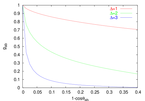
Figure 1: The distribution $g_{ab}$ for $\cos{\theta}_{\mbox{\scriptsize in}}=\mbox{\small$\frac{1}{2}$}$ and $\theta_{a}=0$ as a function of $1\!-\!\cos\theta_{ab}$ for three different values of $\Delta$.

6 Study of the large-$\Delta$ behaviour

We focus on $e^{+}e^{-}$ annihilation with ${\cal C}_{\mbox{\scriptsize in}}$ given by a cone of size ${\theta}_{\mbox{\scriptsize in}}$ around the two jets along thrust axis, see (2). We then generalize this analysis to the distribution $G_{p_{i}p_{j}}$ required for other hard processes, in which the two jets are not back-to-back. To obtain $G_{ab}(\Delta)$ in the large $\Delta$ limit we need first to study its behaviour near the peak at $a\!=\!b$. Using this information we can obtain the asymptotic behaviour of $G_{ab}$ for any $a,b$. These two stages are described in the next two subsections. In a final subsection we consider the particular case of ${\cal C}_{\mbox{\scriptsize in}}$ being a pair of small cones.

6.1 Shape of the peak at $a\!=\!b$

For each point $a$ inside the jet region ${\cal C}_{\mbox{\scriptsize in}}$, we can measure the width of the peak in $b$ near $a$ by using

$$\int_{{\cal C}_{\mbox{\scriptsize in}}}\frac{d^{2}\Omega_{b}}{4\pi}\,G_{ab}(\Delta)\equiv 1-\cos\theta_{\rm crit}(\Delta)\approx\mbox{\small$\frac{1}{2}$}\theta_{\rm crit}^{2}(\Delta)\>.$$ (35)

In general this quantity depends on the geometry of the ${\cal C}_{\mbox{\scriptsize in}}$ region and on the point $a$ chosen in ${\cal C}_{\mbox{\scriptsize in}}$. Here $\theta_{\rm crit}(\Delta)$ measures the angle between $a$ and $b$ above which the distribution $G_{ab}$ is suppressed. It is therefore a small angle which decreases as $\Delta$ increases. We have the initial value $\theta_{\rm crit}(\Delta\!=\!0)\!=\!{\theta}_{\mbox{\scriptsize in}}$.

Since the evolution of the peak is determined only by the distribution around the peak, and not by points remote in phase-space, we have that the shape of the peak in $G_{ab}(\Delta)$ depends only on the angle $\theta_{ab}$ between $a$ and $b$. To measure this shape, suppose that at large $\Delta$ and in the region near $a=b$ the distribution behaves as

$$G_{ab}(\Delta)=h_{\Delta}(z)\>,\qquad z\>=\>\frac{\theta_{ab}^{2}}{2\theta_{\rm crit}^{2}(\Delta)}\>,$$ (36)

for some function $h_{\Delta}(z)$ that from (35) for all large $\Delta$ must satisfy

$$\int_{0}^{\infty}dz\,h_{\Delta}(z)=1\>.$$ (37)

The evolution equation (19) simplifies in that the source term involving $r_{ab}$ is negligible and the integration over solid angle becomes an integration over a flat plane:

$$\begin{split}&\partial_{\Delta}h_{\Delta}(z)-\frac{d\ln\theta_{\rm crit}^{2}}{d\Delta}\cdot zh_{\Delta}^{\prime}(z)=\frac{1}{2\pi}\int\frac{dx\,dy}{r_{1}^{2}r_{2}^{2}}\left[h_{\Delta}(r_{1}^{2}z)h_{\Delta}(r_{2}^{2}z)-h_{\Delta}(z)\right]\>,\\ &r_{1}^{2}=x^{2}+y^{2}\>,\qquad r_{2}^{2}=(1-x)^{2}+y^{2}\>,\qquad\theta_{ak}=r_{1}\theta_{ab}\>,\qquad\theta_{kb}=r_{2}\theta_{ab}\>.\end{split}$$ (38)

Integrating this equation over $z$ yields

$$\frac{d\ln\theta_{\rm crit}^{2}}{d\Delta}=\frac{1}{2\pi}\int_{0}^{\infty}dz\int\frac{dx\,dy}{r_{1}^{2}r_{2}^{2}}\left[h_{\Delta}(r_{1}^{2}z)h_{\Delta}(r_{2}^{2}z)-h_{\Delta}(z)\right].$$ (39)

Equations (37)-(39) form a coupled system that can be evolved numerically from any suitable starting function $h_{0}(z)$. Here $h_{\Delta}(z)$ is a function of only one variable $z$ while the full distribution $G_{ab}(\Delta)$ is a function of three angles, so the implementation is somewhat easier.

There are many possible choices of starting function $h_{0}(z)$: it need only be bounded between 0 and 1, with $h_{0}(0)=1$, normalised, and sufficiently smooth. We used a selection of such functions, namely

$$h_{0}(z)=e^{-\left[z\Gamma(1+\frac{1}{n})\right]^{n}}\>,\>(n=\mbox{\small$\frac{1}{2}$},1,2,3,4)\>,\qquad h_{0}(z)=\frac{2-z}{2}\Theta(2-z)\>,$$ (40)

all of which showed the same asymptotic behaviour. The evolution (38) settles down to a shape $h_{\infty}(z)$ shown in figure 2, which satisfies the equation

$$\begin{split}&c\cdot zh_{\infty}^{\prime}(z)=\frac{1}{2\pi}\int\frac{dx\,dy}{r_{1}^{2}r_{2}^{2}}\left[h_{\infty}(r_{1}^{2}z)h_{\infty}(r_{2}^{2}z)-h_{\infty}(z)\right]\>,\\ &c\equiv-\frac{d\ln\theta_{\rm crit}^{2}}{d\Delta}=-\frac{1}{2\pi}\int_{0}^{\infty}dz\int\frac{dx\,dy}{r_{1}^{2}r_{2}^{2}}\left[h_{\infty}(r_{1}^{2}z)h_{\infty}(r_{2}^{2}z)-h_{\infty}(z)\right]\approx 2.5\>,\end{split}$$ (41)

with $c$ evaluated with an accuracy of about 10%. This error is due to limitations in the numerical analysis from the finite number of $z$-points, and the numerical integrals performed at each stage, such that evolving using the same starting function but with a different number of points or precision in the integrals converges to a slightly different numerical value for $c$. The step size in $\Delta$ needs to be small enough to prevent instabilities developing before convergence is seen — we found the value 0.02 to be sufficiently small. The stated uncertainty on the value of $c$ is a generous estimate. This error could be improved with a more refined analysis.

We then conclude that $\theta_{\rm crit}(\Delta)$ has the behaviour at large $\Delta$ given in (31) with $\lambda_{a}$ an integration constant which depends on ${\theta}_{\mbox{\scriptsize in}}$ and on the chosen point $a$. The fact that $h_{\infty}(z)$ is finite for any $z$ implies that at large $\Delta$ the distribution $G_{ab}(\Delta)$ for $\theta_{ab}\ll 1$ depends on $\Delta,{\theta}_{\mbox{\scriptsize in}}$ and the point $a$ only through the function $\theta_{\rm crit}(\Delta)$. The function $h_{\infty}(z)$ as well as the constant $c$ is universal.

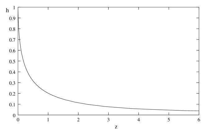
Figure 2: The large $\Delta$ peak, $h_{\infty}(z)$.

From the tail of the function $h_{\infty}(z)$ at large $z$ we can estimate the large-$\Delta$ behaviour of $G_{ab}(\Delta)$ away from the peak in the region

$$\theta_{\rm crit}(\Delta)\ll\theta_{ab}\ll 1\>.$$ (42)

To obtain this we rewrite equation (41) in the form

$$c\cdot\frac{d\ln h_{\infty}}{d\ln z}=\frac{1}{\pi}\int_{r_{1}<r_{2}}\frac{dx\,dy}{r_{1}^{2}r_{2}^{2}}\left[h_{\infty}(r_{1}^{2}z)-1+h_{\infty}(r_{1}^{2}z)\left(\frac{h_{\infty}(r_{2}^{2}z)}{h_{\infty}(z)}-1\right)\right]\>.$$ (43)

As $z\to\infty$ the final term in the brackets vanishes and we obtain

$$c\cdot\frac{d\ln h_{\infty}}{d\ln z}=\int_{0}^{\infty}\frac{dz^{\prime}}{z^{\prime}}\left[h_{\infty}(z^{\prime})-1\right]\,\xi\left(\frac{z^{\prime}}{z}\right)\>,$$ (44)

with

$$\begin{split}\xi(x)=\left\{\begin{split}&\frac{1}{1-x}\>,\qquad\qquad\qquad\qquad\qquad\qquad\qquad\quad x<\frac{1}{4}\>,\\ &\frac{2}{\pi(1-x)}\tan^{-1}\left(\frac{1-\sqrt{x}}{1+\sqrt{x}}\sqrt{\frac{2\sqrt{x}+1}{2\sqrt{x}-1}}\right)\>,\quad x>\frac{1}{4}\>.\end{split}\right.\end{split}$$ (45)

In the large $z$ limit the evolution equation becomes

$$c\cdot\frac{d\ln h_{\infty}}{d\ln z}\simeq-\ln z-c^{\prime}\>,\qquad c^{\prime}=\int_{0}^{1}\frac{dz^{\prime}}{z^{\prime}}\left[1-h_{\infty}(z^{\prime})\right]-\int_{1}^{\infty}\frac{dz^{\prime}}{z^{\prime}}h_{\infty}(z^{\prime})\>.$$ (46)

Therefore, using (31) and (36), we conclude that for $a$ and $b$ in the region (42) we have, in the large $\Delta$ limit,

$$\ln G_{ab}(\Delta)\simeq-\frac{c}{2}\Delta^{2}-\left(c^{\prime}+\ln\frac{\theta_{ab}^{2}}{2\lambda_{a}^{2}}\right)\Delta-\left(\frac{c^{\prime\prime}}{c}+\frac{c^{\prime}}{c}\ln\frac{\theta_{ab}^{2}}{2\lambda_{a}^{2}}+\frac{1}{2c}\ln^{2}\frac{\theta_{ab}^{2}}{2\lambda_{a}^{2}}\right)\>.$$ (47)

The constants $c^{\prime}$ and $c^{\prime\prime}$ can be determined by the function $h_{\infty}(z)$ shown in figure 2. This behaviour is valid provided $a,b$ are away from the boundary of ${\cal C}_{\mbox{\scriptsize in}}$.

In taking the large-$z$ limit, we have neglected terms that contribute at finite $z$ in moving from (43) to (44) and from (44) to (46). The leading correction is ${\cal{O}}\left(z^{-1}\right)$, and arises from the expansion of the $\xi$ function in (44). Thus the right hand side of (47) has a correction ${\cal{O}}\left(e^{-c\Delta}\right)$.

6.2 The distribution off the peak

Using the fact that we know the form of $G_{ab}(\Delta)$ near the peak at $a\!=\!b$, we now determine the large-$\Delta$ behaviour of $G_{ab}(\Delta)$ for any $a$ and $b$ including the physical case in which $a$ and $b$ are along the two hard jet directions ($\theta_{ab}\sim 1$).

We find that the geometry dependence in the integration regions of the two terms in (19) cancels for large $\Delta$. To obtain this result we write (19) in the form

$$\partial_{\Delta}\ln G_{ab}=-\int_{{\cal C}_{\mbox{\scriptsize out}}}\frac{d^{2}\Omega_{k}}{4\pi}\,w_{ab}(k)+\int_{{\cal C}_{\mbox{\scriptsize in}}}\frac{d^{2}\Omega_{k}}{4\pi}w_{ab}(k)\left(\frac{G_{ak}\cdot G_{kb}}{G_{ab}}-1\right)\>.$$ (48)

Since the first term in the second integral is negligible for $k$ not near $a$ or $b$ we may write

$$\begin{split}\partial_{\Delta}\ln G_{ab}\simeq-\int_{\theta_{ak}^{2},\theta_{kb}^{2}>\epsilon}&\frac{d^{2}\Omega_{k}}{4\pi}w_{ab}(k)+\int_{\theta_{ak}^{2}<\epsilon}\frac{d^{2}\Omega_{k}}{4\pi}w_{ab}(k)\left(\frac{G_{ak}\cdot G_{kb}}{G_{ab}}-1\right)\\ &+\int_{\theta_{bk}^{2}<\epsilon}\frac{d^{2}\Omega_{k}}{4\pi}w_{ab}(k)\left(\frac{G_{ak}\cdot G_{kb}}{G_{ab}}-1\right)\>,\end{split}$$ (49)

where $\epsilon$ is a small parameter (larger than $\theta_{\rm crit}$) on which the final answer should not depend. Here we have neglected the ratio ${G_{ak}G_{kb}}/{G_{ab}}$ for $\theta_{ak},\,\theta_{bk}\gg\theta_{\rm crit}$ which vanishes at large $\Delta$. Due to the cancellation of ${\cal C}_{\mbox{\scriptsize in}}$ and ${\cal C}_{\mbox{\scriptsize out}}$ in the integration region, we have that, at large $\Delta$, the distribution $G_{ab}(\Delta)$ depends on the geometry and on the directions of $a$ and $b$ only through ${\theta_{\rm crit}}_{,\,a}(\Delta)$ and ${\theta_{\rm crit}}_{,\,b}(\Delta)$, the critical values in (31).

We now show that the $\epsilon$-dependence in the various terms cancel. The first term of (49) gives the contribution with a cutoff around $a$ and $b$: it is, for small $\epsilon$,

$$\int_{\theta_{ak}^{2},\theta_{kb}^{2}>\epsilon}\frac{d^{2}\Omega_{k}}{4\pi}w_{ab}(k)\simeq\ln\frac{2(1-\cos\theta_{ab})}{\epsilon}\>,$$ (50)

while the second and third terms give the contributions from $k$ near $a$ or $b$, which depend on the shape of the peak given above. We write

$$\int_{\theta_{ak}^{2}<\epsilon}\frac{d^{2}\Omega_{k}}{4\pi}w_{ab}(k)\left(\frac{G_{ak}G_{kb}}{G_{ab}}-1\right)\simeq\frac{1}{2}\int_{0}^{\epsilon}\frac{d\theta_{ak}^{2}}{\theta_{ak}^{2}}\left(G_{ak}-1\right)\simeq-\frac{c^{\prime}}{2}-\frac{1}{2}\ln\frac{\epsilon}{2{\theta_{\rm crit}^{2}}_{,\,a}}\>,$$ (51)

with ${\theta_{\rm crit}}_{,\,a}$ the critical angle for the peak around $a$ and $c^{\prime}$ the constant given in (46). Here corrections vanish in the large $\Delta$ limit. A similar equation holds for the integral around $b$. Thus the $\epsilon$ dependence cancels and we obtain the evolution equation at large $\Delta$:

$$\partial_{\Delta}\ln G_{ab}\simeq-c\Delta-c^{\prime}-\ln\frac{1-\cos\theta_{ab}}{\lambda_{a}\lambda_{b}}\>.$$ (52)

The asymptotic behaviour of $G_{ab}$ is therefore

$$G_{ab}(\Delta)\simeq e^{-\frac{c}{2}\Delta^{2}}\left(\frac{\lambda_{a}\lambda_{b}\,e^{-c^{\prime}}}{1-\cos\theta_{ab}}\right)^{\Delta}f_{ab}({\theta}_{\mbox{\scriptsize in}})\>,$$ (53)

where $f_{ab}$ is independent of $\Delta$ at large $\Delta$. For $\theta_{ab}\ll 1$ we have, see (47),

$$\ln f_{ab}\simeq-\left(\frac{c^{\prime\prime}}{c}+\frac{c^{\prime}}{c}\ln\frac{\theta_{ab}^{2}}{2\lambda_{a}^{2}}+\frac{1}{2c}\ln^{2}\frac{\theta_{ab}^{2}}{2\lambda_{a}^{2}}\right)\>.$$ (54)

Because of this structure, we have that secondary branching is almost collinear to the partons $a,b$ initiating the branching: in fact no farther away than the width of the peak. This implies that as long as $a,b$ are not close to the boundary of ${\cal C}_{\mbox{\scriptsize in}}$ the geometry dependence enters only through the parameter $\lambda_{a}$ in $\theta_{\rm crit}$.

6.3 Small ${\cal C}_{\mbox{\scriptsize in}}$ region

Since the secondary branching is almost collinear to the hard primary partons it becomes interesting to study the limit ${\theta}_{\mbox{\scriptsize in}}\to 0$. In particular we would like to see how the buffer region behaves when the jet region is squeezed. We consider the two cases of $ab$ in the same and in opposite jet regions.

Same jet region.

We derive the evolution equation

$$\begin{split}&\partial_{\Delta}G_{ab}=-r_{ab}\cdot G_{ab}+\int_{|\vec{k}|<1}\frac{d^{2}\vec{k}}{2\pi}\frac{(\vec{a}-\vec{b})^{2}}{(\vec{a}-\vec{k})^{2}(\vec{k}-\vec{b})^{2}}\>\left[G_{ak}\,G_{kb}\,-\,G_{ab}\right]\,,\\ &r_{ab}=\frac{1}{2}\ln\left(1+\frac{(\vec{a}-\vec{b})^{2}}{(1-a^{2})(1-b^{2})}\right)\>,\qquad\vec{a}=\frac{\theta_{a}}{{\theta}_{\mbox{\scriptsize in}}}\,\vec{n}_{a}\>,\qquad\vec{b}=\frac{\theta_{b}}{{\theta}_{\mbox{\scriptsize in}}}\,\vec{n}_{b}\>,\end{split}$$ (55)

using rescaled angular variables $\vec{a},\vec{b}$. The contribution to the evolution of $G_{ab}$ from the branching in the opposite region vanishes for ${\theta}_{\mbox{\scriptsize in}}\to 0$. This is an aspect of coherence of the QCD radiation. We notice that the explicit ${\theta}_{\mbox{\scriptsize in}}$ dependence has disappeared from the equation. This implies that $\theta_{\rm crit}(\Delta)$ scales with ${\theta}_{\mbox{\scriptsize in}}$ so that

$$\lambda_{a}({\cal C}_{\mbox{\scriptsize in}})={\theta}_{\mbox{\scriptsize in}}\cdot\hat{\lambda}(\vec{a})\>,$$ (56)

giving (33) in the case $\vec{a}=0$. We have then that the buffer region still expands by increasing $\Delta$. By performing the same analysis as in subsection 6.1 we find, at large $\Delta$, for $ab$ in the same jet region but away from the peak, the behaviour

$$G_{ab}(\Delta)\simeq e^{-\frac{c}{2}\Delta^{2}}\left(\frac{2\hat{\lambda}(\vec{a})\,\hat{\lambda}(\vec{b})\,e^{-c^{\prime}}}{(\vec{a}-\vec{b})^{2}}\right)^{\Delta}\hat{f}(\vec{a},\vec{b})\>.$$ (57)

Opposite jet regions.

We introduce now rescaled angular variables for the two back-to-back jets (left and right jet). For ${\theta}_{\mbox{\scriptsize in}}\to 0$ the radiator is

$$r_{ab}=-2\ln\frac{{\theta}_{\mbox{\scriptsize in}}}{2}-\frac{1}{2}\ln(1\!-\!a^{2})-\frac{1}{2}\ln(1\!-\!b^{2})\>,\qquad\vec{a}=\frac{\theta_{a}}{{\theta}_{\mbox{\scriptsize in}}}\,\vec{n}_{a}\>,\quad\vec{b}=\frac{\pi-\theta_{b}}{{\theta}_{\mbox{\scriptsize in}}}\,\vec{n}_{b}\>.$$ (58)

This explicit ${\theta}_{\mbox{\scriptsize in}}$ dependence implies that $G_{ab}(\Delta)$ is given by ${\theta}_{\mbox{\scriptsize in}}^{2\Delta}$ (the bremsstrahlung contribution) times a function of the rescaled variables $\vec{a},\vec{b}$, whereas the same jet distribution depends only on the rescaled quantities.

The $a$ and $b$ contributions enter (58) independently. This is due to the fact that $w_{ab}(k)$ splits into a sum of right and left pieces. As a consequence the evolution in the right and left regions develops independently and $G_{ab}(\Delta)$ factorizes

$$G_{ab}(\Delta)\simeq\left(\frac{{\theta}_{\mbox{\scriptsize in}}}{2}\right)^{2\Delta}\cdot F^{\rm R}_{a}(\Delta)\cdot F^{\rm L}_{b}(\Delta)\>.$$ (59)

Here $F^{\rm R}_{a}$ and $F^{\rm L}_{b}$ satisfy the right and left evolutions and for the first we find

$$\partial_{\Delta}F_{a}^{\rm R}=\frac{1}{2}\ln(1-a^{2})\cdot F_{a}^{\rm R}+\int\frac{d^{2}\vec{k}}{2\pi\,(\vec{a}-\vec{k})^{2}}\>\left[G_{ak}^{{\rm RR}}\,F_{k}^{\rm R}\,-\,F_{a}^{\rm R}\right]\,,$$ (60)

where $G_{ak}^{{\rm RR}}$ is the distribution for $a$ and $k$ in the same (right) jet region discussed above. Proceeding as in subsection 6.2 we find the following asymptotic behaviour for the distribution with $ab$ in opposite jet regions

$$G_{ab}(\Delta)\simeq e^{-\frac{c}{2}\Delta^{2}}\left(\frac{{\theta}_{\mbox{\scriptsize in}}^{2}\,\hat{\lambda}(\vec{a})\,\hat{\lambda}(\vec{b})\,e^{-c^{\prime}}}{2}\right)^{\Delta}\>\hat{f}(\vec{a})\hat{f}(\vec{b})\>,$$ (61)

with $c^{\prime}$ the integration constant given in (46) and $\hat{f}$ an integration constant depending only on the rescaled variable. This expression shows that for small ${\theta}_{\mbox{\scriptsize in}}$ the function $f_{ab}({\theta}_{\mbox{\scriptsize in}})$ in (53) factorizes and depends on the rescaled variables. The ${\theta}_{\mbox{\scriptsize in}}$-dependence is the one given by the bremsstrahlung contribution. The secondary branching contribution does not depend on ${\theta}_{\mbox{\scriptsize in}}$ and is decreasing with $\Delta$ with a Gaussian behaviour. For the physical $e^{+}e^{-}$ distribution we set $a^{2}=b^{2}=0$.

A generalization of this result is to the case where the two jets $p_{i}p_{j}$ are not back-to-back but are set at an angle $\theta_{ij}$. The asymptotic behaviour is given by the expression (61) with $\{2\}^{-\Delta}$ replaced by $\{1-\cos\theta_{ij}\}^{-\Delta}$ and with $\theta_{a}$ the angle of $a$ with respect to the jet $p_{i}$ and $\theta_{b}$ the angle of $b$ with $p_{i}$. The physical distribution $G_{p_{i}p_{j}}(\Delta)$ is again obtained by setting $a^{2}\!=\!b^{2}\!=\!0$.

7 Discussion

We summarize here the essential physical points of our results on energy flow away from hard jets. The interjet distribution reduces to $G_{p\bar{p}}(\Delta)$ in (10) for $e^{+}e^{-}$, while for DIS and hadron-hadron collisions it is given in terms of $G_{p_{i}p_{j}}(\Delta)$, see (70) and (76). These distributions depend on the geometry of ${\cal C}_{\mbox{\scriptsize out}}$ and on the jet directions.

A characteristic of interjet observables is that the leading contribution to their distributions are SL, originating from soft emission at large angles. Collinear singularities here are subleading. The contribution from bremsstrahlung emission from the primary hard partons does not give the full SL structure. Indeed we find (see (20))

$$G_{p_{i}p_{j}}(\Delta)=e^{-R^{(0)}_{p_{i}p_{j}}(\Delta)}\cdot g_{p_{i}p_{j}}(\Delta)\>,$$ (62)

with $R^{(0)}_{p_{i}p_{j}}(\Delta)$ the SL Sudakov radiator for emission into ${\cal C}_{\mbox{\scriptsize out}}$. The additional SL factor $g_{p_{i}p_{j}}$ is generated by soft secondary emission, which can be described by successive colour singlet soft dipole emission. This implies that, in the present formulation, we work in the large $N_{c}$ approximation. The soft secondary branching develops with decreasing energy inside the unobserved jet region ${\cal C}_{\mbox{\scriptsize in}}$ until a soft gluon enters ${\cal C}_{\mbox{\scriptsize out}}$. The emission is also effectively angular ordered.

At large $\Delta$ the distribution $G_{p_{i}p_{j}}(\Delta)$ decreases with a universal Gaussian behaviour, see equation (32), with a process-independent coefficient $c$ that we have estimated to be $c\approx 2.5$ with a $10\%$ accuracy. Since the bremsstrahlung radiator is proportional to $\Delta$ we see that the large $\Delta$ behaviour is dominated by the soft secondary branching contribution $g_{p_{i}p_{j}}(\Delta)$.

The origin of the universal Gaussian behaviour in $\Delta$ is a consequence of the structure of the branching. The secondary branching generating $g_{p_{i}p_{j}}(\Delta)$ develops within a small cone $\theta_{\rm crit}(\Delta)$ around the hard primary partons $p_{i}$ and $p_{j}$, which decreases exponentially for large $\Delta$ according to (31), again governed by the universal coefficient $c$. It is the development of soft secondary branching in this peak region which generates the Gaussian behaviour in (32). At large $\Delta$ the region within $\theta_{\rm crit}(\Delta)$ shrinks generating an empty buffer region first observed in [2]. For the case of figure 1 we have estimated that the asymptotic regime sets in around $\Delta=3$. At this value the distribution is negligible away from the peak and approaches the asymptotic limit of figure 2.

Taking the jet region ${\cal C}_{\mbox{\scriptsize in}}$ to be an arrangement of small cones centred on each hard jet leads to a universal secondary emission function $g(\Delta)$ that depends neither on the size of the cones nor on the directions of the jets (see (34)).

The distribution $G_{p_{i}p_{j}}(\Delta)$ is a function of $E,E_{\mbox{\scriptsize out}}$ and the coupling $\alpha_{\mbox{\scriptsize s}}$ through the quantity $\Delta$ defined in (17). This involves an integral over the running coupling at low scales, and so acquires non-perturbative power corrections. These corrections can be estimated by the same method [14] used for the standard shape variables in $e^{+}e^{-}$ and are expressed in term of a unique parameter $\lambda^{\mbox{\scriptsize NP}}$ given by the integral over the running coupling in the low energy region. We obtain

$$\Delta\equiv\int_{0}^{E}\frac{d\omega}{\omega}{\bar{\alpha}_{\mbox{\scriptsize s}}}(\omega)\,[1-e^{-\omega/E_{\mbox{\scriptsize out}}}]\simeq\int_{E_{\mbox{\scriptsize out}}}^{E}\frac{d\omega}{\omega}{\bar{\alpha}_{\mbox{\scriptsize s}}}(\omega)+N_{c}\frac{\lambda^{\mbox{\scriptsize NP}}}{2E_{\mbox{\scriptsize out}}}\>.$$ (63)

The non-perturbative parameter $\lambda^{\mbox{\scriptsize NP}}$ (for the normalization used here see [15]) is measured both at LEP [16] and at HERA [17].

In hadron-hadron collisions one expects [1, 5, 12] additional large contributions to interjet observables coming from a soft underlying event generated by the incoming hadrons. We can write

$$E_{\mbox{\scriptsize out}}=\sum_{i\in{\cal C}_{\mbox{\scriptsize out}}}\omega_{i}+E_{\mbox{\scriptsize out}}^{\rm soft}\>,$$ (64)

where the sum includes all partons produced in the hard process, and the quantity $E_{\mbox{\scriptsize out}}^{\rm soft}$ is the contribution of the soft underlying event. Assuming the underlying emission and hard emission factorize, the final answer will be given by the distribution studied here with the replacement

$$\Delta(E,E_{\mbox{\scriptsize out}})\to\Delta(E,E_{\mbox{\scriptsize out}}-E_{\mbox{\scriptsize out}}^{\rm soft})\>.$$ (65)

Up to now in hadron-hadron collisions only the mean value of $E_{\mbox{\scriptsize out}}$ has been investigated both theoretically and experimentally. One shows that the hard contribution, which can be reliably computed by fixed order QCD calculation, does not fit the data [1, 4, 5] but requires a sizable $E_{\mbox{\scriptsize out}}^{\rm soft}$ contribution.

The resummed PT distribution here discussed provides a way to further study the underlying event, in particular its factorization properties and its size.

Appendix A Interjet observables in DIS and hadron-hadron collisions

We introduce first the physical observables and then the QCD resummation.

A.1 The observable

An example of an interjet distribution in DIS is given by

$$\Sigma_{\rm DIS}(E_{\mbox{\scriptsize out}})=\left\{\sum_{n}\int\frac{d\sigma_{n}}{dx_{\rm B}\,dQ^{2}}\right\}^{-1}\sum_{n}\int\frac{d\sigma_{n}}{dx_{\rm B}\,dQ^{2}}\cdot\Theta\!\left({E}_{\mbox{\scriptsize out}}-\sum_{h\,\in\,{\cal C}_{\mbox{\scriptsize out}}}\omega_{h}\right),$$ (66)

with $d\sigma_{n}/dx_{\rm B}dQ^{2}$ the $n$-hadron distribution for fixed Bjorken variable $x_{\rm B}$ and $Q^{2}$. The events are dominated by the incoming and the outgoing hard jet. In the Breit frame the situation is similar to $e^{+}e^{-}$ with both jets aligned along the beam direction. We may define the ${\cal C}_{\mbox{\scriptsize out}}$ region by

$$-\eta^{(-)}_{\rm in}\><\>\ln\tan\frac{\theta_{h}}{2}\><\>\eta^{(+)}_{\rm in}\>.$$ (67)

An example of an interjet distribution in hadron-hadron collisions with hard jets is

$$\Sigma_{\rm hh}(E_{\mbox{\scriptsize out}})=\left\{\sum_{n}\int\frac{d\sigma_{n}}{d\eta\,dP_{t}}\right\}^{-1}\sum_{n}\int\frac{d\sigma_{n}}{d\eta\,dP_{t}}\cdot\Theta\!\left({E}_{\mbox{\scriptsize out}}-\sum_{h\,\in\,{\cal C}_{\mbox{\scriptsize out}}}\omega_{h}\right),$$ (68)

with $d\sigma_{n}/d\eta dP_{t}$ the $n$-hadron distribution associated to the emission of a jet with rapidity $\eta$ and transverse momentum $P_{t}$. The jet could be defined by a $k_{t}$-jet finding algorithm [19]. Here the event is dominated by the presence of an additional recoiling outgoing jet. The interjet region ${\cal C}_{\mbox{\scriptsize out}}$ should be defined by avoiding the two incoming and the two outgoing hard jets. It is given for instance by fixing a region in the rapidity $\eta_{h}$ and azimuthal angle $\phi_{h}$ of emitted hadrons with respect to the triggered jet, see [4, 5] .

The QCD resummation discussed for $e^{+}e^{-}$ annihilation in section 3 can be generalized to the above processes due to the factorization of the parton process (see for instance [20]) as we shall discuss.

A.2 QCD resummation: DIS case

To express the result for $\Sigma_{\rm DIS}(E_{\mbox{\scriptsize out}})$ we write the DIS cross section in the form

$$\frac{d\sigma}{dx_{\rm B}dQ^{2}}=\int dx_{1}\,\frac{d\sigma_{\gamma+p_{1}\to p_{2}}(x_{1},\mu)}{dx_{1}dx_{\rm B}dQ^{2}}\>,\quad\mu\sim Q\>,$$ (69)

where $d\sigma_{\gamma+p_{1}\to p_{2}}(x_{1},\mu)$ is the factorized parton distribution including the parton density function at the hard scale $\mu\sim Q$ and the squared matrix element of the hard vertex $\gamma^{*}+p_{1}\to p_{2}$. Here $x_{1}$ is the momentum fraction of the hard parton $p_{1}$ coming into the hard vertex in the Breit frame. In the soft limit $p_{1}$ and $p_{2}$ correspond to the directions of the incoming and outgoing jets respectively.

By performing the same analysis as done in section 3 we obtain

$$\Sigma_{\rm DIS}(E_{\mbox{\scriptsize out}})=\left\{\frac{d\sigma}{dx_{\rm B}dQ^{2}}\right\}^{-1}\!\!\!\int dx_{1}\,\frac{d\sigma_{\gamma+p_{1}\to p_{2}}(x_{1},\mu)}{dx_{1}dx_{\rm B}dQ^{2}}\cdot G_{p_{1}p_{2}}(Q,E_{\mbox{\scriptsize out}})\>.$$ (70)

The factorization scale remains at $\mu$ since no observation is made in the collinear region. Here $G_{p_{1}p_{2}}(Q,E_{\mbox{\scriptsize out}})$ is the distribution introduced in (11) with $p_{1}p_{2}$ aligned, in the Breit frame, along the beam direction.

A.3 QCD resummation: hadron-hadron case

The situation here is more involved since we have four jets (two outgoing and two incoming). There are various hard elementary processes

$$p_{1}+p_{2}\>\to\>p_{3}+p_{4}\>,$$ (71)

according to the nature ($q,\bar{q}$ or $g$) of the four involved partons. They are:

$$\begin{split}{\rm A}\qquad&\>q(p_{1})+q^{\prime}(p_{2})\>\to\>q(p_{3})+q^{\prime}(p_{4})\>,\\ {\rm B}\qquad&\>q(p_{1})+q(p_{2})\>\to\>q(p_{3})+q(p_{4})\>,\\ {\rm C}\qquad&\>q(p_{1})+\bar{q}(p_{2})\>\to\>g(p_{3})+g(p_{4})\>,\\ {\rm D}\qquad&\>g(p_{1})+g(p_{2})\>\to\>g(p_{3})+g(p_{4})\>,\end{split}$$ (72)

together with those obtained by crossing transformations.

Energy flow in interjet regions for this process has been studied in [3] as far as the SL bremsstrahlung radiator piece. To construct the SL contribution from the soft secondary branching we need to represent the soft $n$-gluon emission in each of the hard processes (71) as a combination of colour singlet dipole emissions (6) from the four hard partons. The square amplitude for the emission in (71) of a single soft gluon $k$ has been written in [21]. Taking the large $N_{c}$ limit, this result can be expressed [22] as a sum of dipole emissions $w_{ij}(k)$ from pairs $p_{i}p_{j}$ of hard partons with the factorized structure

$$M^{2}_{f_{1}f_{2}f_{3}f_{4}\,,k}\to M^{2}_{f_{1}f_{2}f_{3}f_{4}}\cdot\sum_{\gamma}C^{(\gamma)}_{f_{1}f_{2}f_{3}f_{4}}\sum_{\left\langle ij\right\rangle\,\in\,\gamma}\frac{{\bar{\alpha}_{\mbox{\scriptsize s}}}}{\omega_{k}^{2}}\,w_{ij}(k)\>,\qquad\sum_{\gamma}C^{(\gamma)}_{f_{1}f_{2}f_{3}f_{4}}=1\>,$$ (73)

where $M^{2}_{f_{1}f_{2}f_{3}f_{4}}$ is the exact hard elementary $2\!\to\!2$ distribution for the process (71) with $f_{i}$ the type of parton $p_{i}$. The coefficients $C^{(\gamma)}_{f_{1}f_{2}f_{3}f_{4}}$ are functions of the kinematical invariants $\hat{s}\!=\!(p_{1}\!+\!p_{2})^{2}$ , $\hat{t}\!=\!(p_{1}\!-\!p_{3})^{2}$, $\hat{u}\!=\!(p_{1}\!-\!p_{4})^{2}$ and can be found in [22]. Here $\gamma$ represents the set of all colour-connected partons in the specific hard process and the last sum is over all colour connected pairs $ij$ in the set $\gamma$.

The simplest process is $qq^{\prime}\to qq^{\prime}$ with only $\left\langle f_{1}f_{4}\right\rangle$ and $\left\langle f_{2}f_{3}\right\rangle$ colour connections. Here the coefficients are independent of the invariants and, from symmetry, we have

$$\sum_{\gamma}C^{(\gamma)}_{qq^{\prime}qq^{\prime}}\sum_{\left\langle ij\right\rangle\in\gamma}w_{ij}(k)=w_{14}(k)+w_{23}(k)\>.$$ (74)

The most complex process is $gg\to gg$ for which all possible colour connections contribute.

The distribution for the emission in the hard process (71) of $n$ additional soft gluons in the strongly energy ordered region is obtained by performing the analysis done in [7, 11] in the large $N_{c}$ limit. Each additional soft gluon contributes to one of the hard dipole emissions as done in (6). This allows us to extend the analysis of section 3 and deduce the interjet $E_{\mbox{\scriptsize out}}$ distribution in hadron-hadron collisions with a hard jet of rapidity $\eta$ and transverse momentum $P_{t}$.

Consider the hadronic cross section for this process which we write in the form

$$\frac{d\sigma}{d\eta dP_{t}}=\sum_{\{f_{i}\}}\int dx_{1}dx_{2}\frac{d\sigma_{f_{1}f_{2}\to f_{3}f_{4}}(x_{1}x_{2},\mu)}{dx_{1}dx_{2}d\eta dP_{t}}\>,\quad\mu\sim P_{t}\>,$$ (75)

where $d\sigma_{f_{1}f_{2}\to f_{3}f_{4}}$ is the parton process integrand which includes parton density functions and hard parton distribution $M^{2}_{f_{1}f_{2}f_{3}f_{4}}$ for the elementary process (71). The normalized $E_{\mbox{\scriptsize out}}$ distribution in a given interjet region ${\cal C}_{\mbox{\scriptsize out}}$ is then given by

$$\begin{split}\Sigma_{\rm hh}(E_{\mbox{\scriptsize out}})&=\left\{\frac{d\sigma}{d\eta dP_{t}}\right\}^{-1}\!\!\sum_{\{f_{i}\}}\int dx_{1}dx_{2}\frac{d\sigma_{f_{1}f_{2}\to f_{3}f_{4}}(x_{1}x_{2},\mu)}{dx_{1}dx_{2}d\eta dP_{t}}\Sigma_{f_{1}f_{2}f_{3}f_{4}}(P_{t},E_{\mbox{\scriptsize out}})\>,\\ &\Sigma_{f_{1}f_{2}f_{3}f_{4}}(P_{t},E_{\mbox{\scriptsize out}})=\sum_{\gamma}C^{(\gamma)}_{f_{1}f_{2}f_{3}f_{4}}\prod_{\left\langle ij\right\rangle\,\in\,\gamma}G_{p_{i}p_{j}}(P_{t},E_{\mbox{\scriptsize out}})\>,\end{split}$$ (76)

where $G_{p_{i}p_{j}}(P_{t},E_{\mbox{\scriptsize out}})$ is the distribution introduced in (11) associated with the dipole $p_{i},p_{j}$. In the soft limit we can take $p_{1}p_{2}$ in the direction of the two incoming hadrons and $p_{3}p_{4}$ in the direction of the two outgoing hard jets. We report the explicit form of $\Sigma_{f_{1}f_{2}f_{3}f_{4}}(P_{t},E_{\mbox{\scriptsize out}})$ for the elementary processes in (72):

$$\begin{split}H^{\rm A}\,\Sigma^{\rm A}&\!=\!h^{\rm A}(\hat{s},\hat{t},\hat{u})\,G_{14}G_{23}\>,\\ H^{\rm B}\,\Sigma^{\rm B}&\!=\!h^{\rm B}(\hat{s},\hat{t},\hat{u})\>G_{14}G_{23}+h^{\rm B}(\hat{s},\hat{u},\hat{t})\>G_{13}G_{24}\,,\\ H^{\rm C}\,\Sigma^{\rm C}&\!=\!h^{\rm C}(\hat{s},\hat{t},\hat{u})\>G_{34}G_{13}G_{24}+h^{\rm C}(\hat{s},\hat{u},\hat{t})\>G_{34}G_{14}G_{23}\,,\\ H^{\rm D}\,\Sigma^{\rm D}&\!=\!h^{\rm D}(\hat{s},\hat{t},\hat{u})G_{12}G_{24}G_{43}G_{31}+h^{\rm D}(\hat{s},\hat{u},\hat{t})\>G_{12}G_{23}G_{34}G_{41}\\ &+h^{\rm D}(\hat{u},\hat{t},\hat{s})\>G_{14}G_{42}G_{23}G_{31}\,,\end{split}$$ (77)

with $G_{ij}=G_{p_{i}p_{j}}(P_{t},E_{\mbox{\scriptsize out}})$ and the functions $h^{({\rm A,B,C,D})}$ given in table 1. Here

$$\begin{split}&H^{\rm A}=h^{\rm A}(\hat{s},\hat{t},\hat{u})\,,\\ &H^{\rm B}=h^{\rm B}(\hat{s},\hat{t},\hat{u})+h^{\rm B}(\hat{s},\hat{u},\hat{t})\,,\\ &H^{\rm C}=h^{\rm C}(\hat{s},\hat{t},\hat{u})+h^{\rm C}(\hat{s},\hat{u},\hat{t})\,,\\ &H^{\rm D}=h^{\rm D}(\hat{s},\hat{t},\hat{u})+h^{\rm D}(\hat{s},\hat{u},\hat{t})+h^{\rm D}(\hat{u},\hat{t},\hat{s})\>,\end{split}$$ (78)

are the square amplitudes for the $2\to 2$ elementary processes (72).

$h^{\rm A}(s,t,u)=g^{4}\frac{C_{F}}{N_{c}}\left(\frac{s^{2}+u^{2}}{t^{2}}\right)$ $h^{\rm B}(s,t,u)=h^{\rm A}(s,t,u)+2g^{4}\frac{C_{F}}{N_{c}^{2}}\frac{s}{t}$ $h^{\rm C}(s,t,u)=g^{4}C_{F}\frac{u}{t}\left(\frac{t^{2}+u^{2}}{s^{2}}-\frac{1}{N_{c}^{2}}\right)$ $h^{\rm D}(s,t,u)=2g^{4}\left(\frac{N_{c}^{2}}{N_{c}^{2}-1}\right)\left(1-\frac{tu}{s^{2}}-\frac{su}{t^{2}}+\frac{u^{2}}{st}\right)$

Table 1: The functions $h^{({\rm A,B,C,D})}$ taken from Ref. [22].

The structure in (77) in terms of the factorized distributions $G_{ij}$ is derived from eq. 66 of Ref. [22] in which we have identified $2C_{F}$ with $C_{A}$ since we work in the large $N_{c}$ limit. Going beyond the large $N_{c}$ approximation requires the analysis of colour interference between different hard partons. At the moment this can be done only for the bremsstrahlung contribution, elegantly computed in [3], see also [23].

In conclusion, for all considered hard processes, the interjet distributions are described by the universal function $G_{p_{i}p_{j}}(E,E_{\mbox{\scriptsize out}})$ which depends on the two hard jet directions $p_{i}$ and $p_{j}$ (incoming or outgoing) and on the interjet region ${\cal C}_{\mbox{\scriptsize out}}$.

Appendix B Theorem: $0\leq G_{ab}(\Delta)\leq 1$

In this appendix we show that the solution of the differential equation (19) with the given boundary condition is bounded below and above by 0 and 1. Thus our distribution is physically meaningful.

Proof:

1. $G_{ab}(\Delta)$ is a continuous function of $\Delta$ and of $a$ and $b$.

2. $G_{ab}(0)=1\>\forall\>a,b$.

3. If $a=b$ then $G_{ab}(\Delta)=1\>\forall\>\Delta$.

4. Suppose $\exists\>a^{\prime},b^{\prime}$ and $\Delta^{\prime}$ with $G_{a^{\prime}b^{\prime}}(\Delta^{\prime})>1$. Then by continuity $\exists\>a^{\prime\prime},b^{\prime\prime}$ and $\Delta^{\prime\prime}$ with $0\leq\Delta^{\prime\prime}<\Delta^{\prime}$, $G_{ab}(\Delta^{\prime\prime})\leq 1\>\forall\>a,b$, and $a^{\prime\prime}\neq b^{\prime\prime}$, $G_{a^{\prime\prime}b^{\prime\prime}}(\Delta^{\prime\prime})=1$, $\partial_{\Delta}G_{a^{\prime\prime}b^{\prime\prime}}(\Delta^{\prime\prime})\geq 0$.

5. But by (19) we have $\partial_{\Delta}G_{a^{\prime\prime}b^{\prime\prime}}(\Delta^{\prime\prime})<0$ which gives a contradiction. Therefore $G_{ab}(\Delta)\leq 1\>\forall\>a,b,\Delta$.

6. Suppose now $\exists\>a^{\prime},b^{\prime}$ and $\Delta^{\prime}$ with $G_{a^{\prime}b^{\prime}}(\Delta^{\prime})<0$. Then by continuity $\exists\>a^{\prime\prime},b^{\prime\prime}$ and $\Delta^{\prime\prime}$ with $0\leq\Delta^{\prime\prime}<\Delta^{\prime}$, $G_{ab}(\Delta^{\prime\prime})\geq 0\>\forall\>a,b$, and $a^{\prime\prime}\neq b^{\prime\prime}$, $G_{a^{\prime\prime}b^{\prime\prime}}(\Delta^{\prime\prime})=0$, $\partial_{\Delta}G_{a^{\prime\prime}b^{\prime\prime}}(\Delta^{\prime\prime})\leq 0$.

7. But by (19) we have $\partial_{\Delta}G_{a^{\prime\prime}b^{\prime\prime}}(\Delta^{\prime\prime})>0$ which gives a contradiction. Therefore $G_{ab}(\Delta)\geq 0\>\forall\>a,b,\Delta$.

Appendix C Iterative solution

Here we calculate the first term $R_{p\bar{p}}^{(1)}(\Delta)$ in the iterative solution described in section 5.1. First we have that for any $a,b$ the bremsstrahlung emission is given by

$$\begin{split}r_{ab}&=\frac{s_{a}}{2}\ln\frac{\cos\theta_{a}+\cos{\theta}_{\mbox{\scriptsize in}}}{\cos\theta_{a}-\cos{\theta}_{\mbox{\scriptsize in}}}+\frac{s_{b}}{2}\ln\frac{\cos\theta_{b}+\cos{\theta}_{\mbox{\scriptsize in}}}{\cos\theta_{b}-\cos{\theta}_{\mbox{\scriptsize in}}}+\frac{s_{a}+s_{b}}{4}\times\\ &\ln\frac{(1\!+\!\cos^{2}{\theta}_{\mbox{\scriptsize in}})(1\!+\!\cos\theta_{a}\cos\theta_{b})\!-\!2\cos{\theta}_{\mbox{\scriptsize in}}(\cos\theta_{a}\!+\!\cos\theta_{b})\!-\!\sin^{2}{\theta}_{\mbox{\scriptsize in}}\sin\theta_{a}\sin\theta_{b}\cos\phi_{ab}}{(1\!+\!\cos^{2}{\theta}_{\mbox{\scriptsize in}})(1\!+\!\cos\theta_{a}\cos\theta_{b})\!+\!2\cos{\theta}_{\mbox{\scriptsize in}}(\cos\theta_{a}\!+\!\cos\theta_{b})\!-\!\sin^{2}{\theta}_{\mbox{\scriptsize in}}\sin\theta_{a}\sin\theta_{b}\cos\phi_{ab}},\end{split}$$ (79)

where $s_{k}=1$ for $\cos\theta_{k}>0$ and $s_{k}=-1$ for $\cos\theta_{k}<0$. Therefore we obtain $R_{ab}^{(0)}$ in the following cases

$$\begin{split}&R_{p\bar{p}}^{(0)}(\Delta)=\Delta\cdot\ln\frac{1+\cos{\theta}_{\mbox{\scriptsize in}}}{1-\cos{\theta}_{\mbox{\scriptsize in}}}\>,\\ &R_{pk}^{(0)}(\Delta)=\Delta\cdot\frac{s_{k}}{2}\ln\frac{(1-\cos{\theta}_{\mbox{\scriptsize in}})(\cos\theta_{k}+\cos{\theta}_{\mbox{\scriptsize in}})}{(1+\cos{\theta}_{\mbox{\scriptsize in}})(\cos\theta_{k}-\cos{\theta}_{\mbox{\scriptsize in}})}\>,\\ &R_{k\bar{p}}^{(0)}(\Delta)=\Delta\cdot\frac{s_{k}}{2}\ln\frac{(1+\cos{\theta}_{\mbox{\scriptsize in}})(\cos\theta_{k}+\cos{\theta}_{\mbox{\scriptsize in}})}{(1-\cos{\theta}_{\mbox{\scriptsize in}})(\cos\theta_{k}-\cos{\theta}_{\mbox{\scriptsize in}})}\>.\end{split}$$ (80)

Now using the definition (28) we explicitly calculate

$$R_{p\bar{p}}^{(1)}(\Delta)=\int_{0}^{\Delta}d\Delta^{\prime}\int_{{\cal C}_{\mbox{\scriptsize in}}}\!\frac{d^{2}\Omega_{k}}{4\pi}\,w_{p\bar{p}}(k)\>\left[1-U^{(0)}_{p\bar{p}k}(\Delta^{\prime})\right]\>,$$ (81)

where

$$U^{(0)}_{p\bar{p}k}(\Delta)=\left(\frac{|\cos\theta_{k}|-\cos{\theta}_{\mbox{\scriptsize in}}}{|\cos\theta_{k}|+\cos{\theta}_{\mbox{\scriptsize in}}}\right)^{\Delta}\left(\frac{1+\cos{\theta}_{\mbox{\scriptsize in}}}{1-\cos{\theta}_{\mbox{\scriptsize in}}}\right)^{\Delta}\>.$$ (82)

For large $\Delta$ the integrand $[1-U^{(0)}_{p\bar{p}k}(\Delta)]$ forces $k$ to stay away from the thrust axis by an small angle of order $\Delta^{-1}$. Changing integration variables we have

$$R_{p\bar{p}}^{(1)}(\Delta)=\int_{0}^{\Delta}d\Delta^{\prime}\int_{0}^{1}dx\left(\frac{1-x^{\Delta^{\prime}}}{1-x}-\frac{1-x^{\Delta^{\prime}}}{\cot^{4}\frac{{\theta}_{\mbox{\scriptsize in}}}{2}-x}\right)\>.$$ (83)

At small $\Delta$ this gives the result (29), while at large $\Delta$ we obtain (30).

References

- [1] G. Marchesini and B.R. Webber, Phys. Rev. D 38 (1988) 3419.
- [2] M. Dasgupta and G. P. Salam, J. High Energy Phys. 03 (2002) 017 [hep-ph/0203009].
- [3] C. F. Berger, T. Kucs and G. Sterman, Phys. Rev. D 65 (2002) 094031 [hep-ph/0110004].
- [4] UA1 Collaboration, C. Albajar et al. Nucl. Phys. B 309 (1988) 405.
-
[5]
J. Huston and V. Tano, in “The QCD and standard model working group:
Summary report”, hep-ph/0005114;
R. D. Field [CDF Collaboration], hep-ph/0201192;
W. Giele et al., “The QCD/SM working group: Summary report”, hep-ph/0204316. -
[6]
A.H. Mueller,
Phys. Lett. B 104 (1981) 161;
B. I. Ermolaev and V. S. Fadin, JETP Lett. 33, 269 (1981) [Pisma Zh. Eksp. Teor. Fiz. 33, 285 (1981)];
A. Bassetto, M. Ciafaloni, G. Marchesini and A. H. Mueller, Nucl. Phys. B 207 (1982) 189;
Y. L. Dokshitzer, V. A. Khoze, A. H. Mueller and S. I. Troyan, Gif-sur-Yvette, France: Ed. Frontieres (1991) 274 p. (Basics of perturbative QCD). - [7] A. Bassetto, M. Ciafaloni and G. Marchesini, Phys. Rept. 100 (1983) 201.
-
[8]
S. Catani, L. Trentadue, G. Turnock and B.R. Webber,
Nucl. Phys. B 407 (1993) 3;
S. Catani and B.R. Webber, Phys. Lett. B 427 (1998) 377 [hep-ph/9801350];
Yu.L. Dokshitzer, A. Lucenti, G. Marchesini and G.P. Salam, J. High Energy Phys. 01 (1998) 011 [hep-ph/9801324]. -
[9]
L.N. Lipatov, Sov. J. Nucl. Phys. 20 (1975) 94;
V.N. Gribov and L.N. Lipatov, Sov. J. Nucl. Phys. 15 (1972) 438;
G. Altarelli and G. Parisi, Nucl. Phys. B 126 (1977) 298;
Yu.L. Dokshitzer Sov. Phys. JETP 46 (1977) 641. - [10] M. Dasgupta and G. P. Salam, Phys. Lett. B 512 (2001) 323 [hep-ph/0104277].
- [11] F. Fiorani, G. Marchesini and L. Reina, Nucl. Phys. B 309 (1988) 439.
-
[12]
G. Corcella, I.G. Knowles, G. Marchesini, S. Moretti, K. Odagiri,
P. Richardson, M.H. Seymour, B.R. Webber,
J. High Energy Phys. 01 (2001) 010 [hep-ph/0011363];
T. Sjostrand, Comput. Phys. Commun. 82 (1994) 74;
L. Lonnblad, Comput. Phys. Commun. 71 (1992) 15. - [13] S. Catani, G. Marchesini and B.R. Webber, Nucl. Phys. B 349 (1991) 635.
-
[14]
B.R. Webber, Phys. Lett. B 339 (1994) 148 [hep-ph/9408222];
M. Beneke and V.M. Braun, Nucl. Phys. B 454 (1995) 253 [hep-ph/9506452];
Yu.L. Dokshitzer and B.R. Webber, Phys. Lett. B 352 (1995) 451 [hep-ph/9504219];
R. Akhoury and V.I. Zakharov, Phys. Lett. B 357 (1995) 646 [hep-ph/9504248]; Nucl. Phys. B 465 (1996) 295 [hep-ph/9507253];
G.P. Korchemsky and G. Sterman, Nucl. Phys. B 437 (1995) 415 [hep-ph/9411211];
Yu.L. Dokshitzer, V.A. Khoze and S.I. Troyan, Phys. Rev. D 53 (1996) 89 [hep-ph/9506425];
P. Nason and M.H. Seymour, Nucl. Phys. B 454 (1995) 291 [hep-ph/9506317];
Yu.L. Dokshitzer, G. Marchesini and B.R. Webber, Nucl. Phys. B 469 (1996) 93 [hep-ph/9512336];
M. Beneke, Phys. Rept. 317 (1999) 1 [hep-ph/9807443]. - [15] A. Banfi, G. Marchesini and G. Smye, J. High Energy Phys. 04 (2002) 024 [hep-ph/0203150].
-
[16]
P. A. Movilla Fernandez, O. Biebel, S. Bethke,
paper contributed to the EPS-HEP99 conference in Tampere, Finland,
hep-ex/9906033.
H. Stenzel, MPI-PHE-99-09 Prepared for 34th Rencontres de Moriond: “QCD and Hadronic interactions”, Les Arcs, France, 20-27 Mar 1999;
ALEPH Collaboration, “QCD Measurements in e+e- Annihilations at Centre-of-Mass Energies between 189 and 202 GeV”, ALEPH 2000-044 CONF 2000-027;
P. Abreu et al. (DELPHI Collaboration), Phys. Lett. B 456 (1999) 322;
DELPHI Collaboration, “The Running of the Strong Coupling and a Study of Power Corrections to Hadronic Event Shapes with the DELPHI Detector at LEP”, DELPHI 2000-116 CONF 415, July 2000.
M. Acciarri et al. (L3 Collaboration), Phys. Lett. B 489 (2000) 65 [hep-ex/0005045]. -
[17]
C. Adloff et al. [H1 Collaboration],
Eur. Phys. J. C 14 (2000) 255, erratum ibid. C18 (2000) 417
[hep-ex/9912052];
G. J. McCance [H1 collaboration], hep-ex/0008009. -
[18]
Z. Bern , L.J. Dixon, and D.A. Kosower,
Phys. Rev. Lett. 70 (1993) 2677 [hep-ph/9302280];
Nucl. Phys. B 437 (1995) 259 [hep-ph/9409393];
Z. Kunszt , A. Signer, and Z. Trócsányi, Phys. Lett. B 336 (1994) 529 [hep-ph/9405386];
J.G.M. Kuijf , Ph.D. thesis, Universiteit Leiden, 1991;
J.F. Gunion and Z. Kunszt, Phys. Lett. B 159 (1985) 167; Phys. Lett. B 176 (1986) 477; Phys. Lett. B 176 (1986) 163;
Z. Nagy, Phys. Rev. Lett. 88 (2002) 122003 [hep-ph/0110315]. -
[19]
S. Catani, Y. L. Dokshitzer and B. R. Webber,
Phys. Lett. B 285 (1992) 291;
S. Catani, Y. L. Dokshitzer, M. H. Seymour and B. R. Webber, Nucl. Phys. B 406 (1993) 187. -
[20]
J. C. Collins, D. E. Soper and G. Sterman,
Nucl. Phys. B 26 (1985) 104;
G. T. Bodwin, Phys. Rev. D 31 (1985) 2616, erratum ibid. D34 (1986) 3932. - [21] R. K. Ellis, G. Marchesini and B. R. Webber, Nucl. Phys. B 286 (1987) 643, erratum ibid. B294 (1987) 1180.
- [22] G. Marchesini and B. R. Webber, Nucl. Phys. B 310 (1988) 461,
-
[23]
N. Kidonakis and G. Sterman,
Nucl. Phys. B 505 (1997) 321 [hep-ph/9705234];
N. Kidonakis, G. Oderda and G. Sterman, Nucl. Phys. B 531 (1998) 365 [hep-ph/9803241].