The LMA Solution from Bimaximal Lepton Mixing at the GUT Scale by Renormalization Group Running

Abstract

We show that in see-saw models with bimaximal lepton mixing at the GUT scale and with zero CP phases, the solar mixing angle $\theta_{12}$ generically evolves towards sizably smaller values due to Renormalization Group effects, whereas the evolution of $\theta_{13}$ and $\theta_{23}$ is comparatively small. The currently favored LMA solution of the solar neutrino problem can thus be obtained in a natural way from bimaximal mixing at the GUT scale. We present numerical examples for the evolution of the leptonic mixing angles in the Standard Model and the MSSM, in which the current best-fit values of the LMA mixing angles are produced. These include a case where the mass eigenstates corresponding to the solar mass squared difference have opposite CP parity.

TUM-HEP-466/02

, , ,

1 Introduction

Recent experimental evidence strongly favors the LMA solution of the solar neutrino problem with a large but non-maximal value of the solar mixing angle $\theta_{12}$ [1, 2, 3, 4]. An overview of the current allowed regions for the mixing angles and the mass squared differences is given in table 1.

	Best-fit value	Range (for $\theta\in[0^{\circ},45^{\circ}]$)	C.L.
$\theta_{12}$ [${\>}^{\circ}$]	$32.9$	$26.1-43.3$	$99\%\;(3\sigma)$
$\theta_{23}$ [${\>}^{\circ}$]	$45.0$	$33.2-45.0$	$99\%\;(3\sigma)$
$\theta_{13}$ [${\>}^{\circ}$]	$-$	$0.0-9.2$	$90\%\;(2\sigma)$
$\Delta m^{2}_{\mathrm{sol}}$ [eV2]	$5\cdot 10^{-5}$	$2.3\cdot 10^{-5}-3.7\cdot 10^{-4}$	$99\%\;(3\sigma)$
$|\Delta m^{2}_{\mathrm{atm}}|$ [eV2]	$2.5\cdot 10^{-3}$	$1.2\cdot 10^{-3}-5\cdot 10^{-3}$	$99\%\;(3\sigma)$

Table 1: Experimental data for the neutrino mixing angles and mass squared differences. For the solar angle $\theta_{12}$ and the solar mass squared difference, the LMA solution has been assumed. The results stem from the analysis of the recent SNO data [3], the Super-Kamiokande atmospheric data [5] and the CHOOZ experiment [6].

A big problem for model builders is to explain the deviation of $\theta_{12}$ from maximal mixing, while keeping $\theta_{23}$ maximal and $\theta_{13}$ small at the same time. The Renormalization Group (RG) evolution is a possible candidate for accomplishing this. Therefore, it is interesting to investigate the evolution of the mixing angles from the GUT scale to the electroweak (EW) or SUSY-breaking scale. A number of studies with three neutrinos considered the possibility of increasing a small mixing angle via RG evolution [7, 8, 9, 10]. Others focused on the case of nearly degenerate neutrinos [11, 12, 13, 14, 15, 16], on the existence of fixed points [17], or on the effect of non-zero Majorana phases on the stability of the RG evolution [18].

We consider the see-saw scenario, i.e. the Standard Model (SM) or MSSM extended by 3 heavy neutrinos that are singlets under the SM gauge groups and have large explicit (Majorana) masses with a non-degenerate spectrum. Due to this non-degeneracy, one has to use several effective theories, with the singlets partly integrated out, when studying the evolution of the effective mass matrix of the light neutrinos [19, 20]. Below the lowest mass threshold, the neutrino mass matrix is given by the effective dimension 5 neutrino mass operator in the SM or MSSM. The relevant RGE’s were derived in [20, 21, 22, 23, 24, 25].

In this paper, we assume bimaximal mixing at the GUT scale with vanishing CP phases and positive mass eigenvalues. We calculate the RG running numerically in order to obtain the mixing angles at low energy and to compare them with the experimentally favored values. We include the regions above and between the see-saw scales in our study, which have not been considered in most of the previous works. We find that the solar mixing angle changes considerably, while the evolution of the other angles is comparatively small, so that values compatible with the LMA solution can be obtained. We present analytic approximations that help to understand this behavior and show that it is rather generic.

2 Bimaximal Mixing at the GUT Scale

At the GUT scale, we assume bimaximal mixing in the lepton sector. We restrict ourselves to the case of positive mass eigenvalues and real parameters, so that there is no CP violation. In the basis where the charged lepton Yukawa matrix is diagonal, up to phase conventions the general parametrization of the effective Majorana mass matrix of the light neutrinos is then

$$m^{\mathrm{bimax}}_{\nu}=V(\tfrac{\pi}{4},0,\tfrac{\pi}{4})\cdot\operatorname{diag}(m_{1},m_{2},m_{3})\cdot V^{T}(\tfrac{\pi}{4},0,\tfrac{\pi}{4})=\left(\begin{array}[]{ccc}a\!-\!b&c&-c\\ c&a&b\\ -c&b&a\\ \end{array}\right)$$ (4)

where

$$V(\theta_{12},\theta_{13},\theta_{23})=\left(\begin{array}[]{ccc}c_{12}c_{13}&s_{12}c_{13}&s_{13}\\ -c_{23}s_{12}-s_{23}s_{13}c_{12}&c_{23}c_{12}-s_{23}s_{13}s_{12}&s_{23}c_{13}\\ s_{23}s_{12}-c_{23}s_{13}c_{12}&-s_{23}c_{12}-c_{23}s_{13}s_{12}&c_{23}c_{13}\end{array}\right)$$ (5)

with $s_{ij}=\sin\theta_{ij}$ and $c_{ij}=\cos\theta_{ij}$ is the (orthogonal) CKM matrix in standard parametrization, and

$$a = \frac{1}{4}\left(m_{1}+m_{2}+2\,m_{3}\right)\;,$$ (6a)

$$b = \frac{1}{4}\left(-m_{1}-m_{2}+2\,m_{3}\right)\;,$$ (6b)

$$c = \frac{m_{2}-m_{1}}{2\sqrt{2}}\;.$$ (6c)

Inverting equations (6) yields the mass eigenvalues

$$m_{1} = a-b-\sqrt{2}\,c\;,$$ (7a)

$$m_{2} = a-b+\sqrt{2}\,c\;,$$ (7b)

$$m_{3} = a+b\;.$$ (7c)

From equation (6a) we see that $a>0$. Equations (7) imply that the solar mass squared difference $\Delta m_{\mathrm{sol}}^{2}=m_{2}^{2}-m_{1}^{2}$ is related to $c$, while the atmospheric one, $\Delta m_{\mathrm{atm}}^{2}=m_{3}^{2}-m_{1}^{2}$, is controlled by $b$. Thus, $a>|b|>|c|$. For $b>0$ we obtain a normal mass hierarchy, while for $b<0$ the mass hierarchy is inverted, as illustrated in figure 1. For positive $c$, $m_{1}<m_{2}$, otherwise $m_{1}>m_{2}$. Hence, $\Delta m_{\mathrm{sol}}^{2}$ is positive only if $c$ is. If $a\gg|b|,|c|$, the spectrum is called degenerate. We use the convention that the mass label 2 is attached in such a way that $0\leq\theta_{12}\leq 45^{\circ}$. This can always be accomplished by the replacement $c\leftrightarrow-c$.

(a) Normal hierarchy

(b) Inverted hierarchy

Figure 1: Possible mass hierarchies for the light neutrinos. We use the convention that $m_{1}$ and $m_{2}$ are chosen in such a way that $0\leq\theta_{12}\leq 45^{\circ}$. The LMA solution then requires $m_{2}>m_{1}$.

In our see-saw scenario, the effective mass matrix of the light neutrinos is

$$m_{\nu}^{\mathrm{bimax}}=\frac{v_{\mathrm{EW}}^{2}}{2}\,Y_{\nu}^{T}M^{-1}Y_{\nu}$$ (8)

at the high-energy scale, with $\left\langle\phi\right\rangle=\frac{v_{\mathrm{EW}}}{\sqrt{2}}\approx 174$ GeV. Obviously, the singlet Yukawa and mass matrices $Y_{\nu}$ and $M$ cannot be determined uniquely from this relation, i.e. there is a set of $\{Y_{\nu},M\}$ configurations that yield bimaximal mixing. After choosing an initial condition for $Y_{\nu}$, $M$ (and thus the see-saw scales) is fixed by the see-saw formula (8) if $Y_{\nu}$ is invertible.

3 Solving the RGE’s

To study the RG running of the leptonic mixing angles and neutrino masses, all parameters of the theory have to be evolved from the GUT scale to the EW or SUSY-breaking scale, respectively. Since the heavy singlets have to be integrated out at their mass thresholds, which are non-degenerate in general, a series of effective theories has to be used. The derivation of the RGE’s and the method for dealing with these effective theories are given in [20]. Starting at the GUT scale, the strategy is to successively solve the systems of coupled differential equations of the form

$$16\pi^{2}\,\mu\frac{\mathrm{d}}{\mathrm{d}\mu}\accentset{(n)}{X}_{i}=\accentset{(n)}{\beta}_{{X}_{i}}\raise 3.0pt\hbox{$\displaystyle\bigl{(}$}\raise 3.0pt\hbox{$\displaystyle\bigl{\{}$}\accentset{(n)}{X}_{j}\raise 3.0pt\hbox{$\displaystyle\bigl{\}}$}\raise 3.0pt\hbox{$\displaystyle\bigl{)}$}$$ (9)

for all the parameters $\accentset{(n)}{X}_{i},\accentset{(n)}{X}_{j}\in\raise 3.0pt\hbox{$\displaystyle\bigl{\{}$}\accentset{(n)}{\kappa},\accentset{(n)}{Y_{\nu}},\accentset{(n)}{M},\dots\raise 3.0pt\hbox{$\displaystyle\bigr{\}}$}$ of the theory in the energy ranges corresponding to the effective theories denoted by $(n)$. At each see-saw scale, tree-level matching is performed. Due to the complicated structure of the set of differential equations, the exact solution can only be obtained numerically. However, to understand certain features of the RG evolution, an analytic approximation at the GUT scale will be derived in section 5.

4 Examples for the Running of the Mixing Angles

Figures 2 and 3 show typical numerical examples for the running of the mixing angles from the GUT scale to the EW or SUSY-breaking scale. They contain an important effect that appears for most choices of the initial parameters: The solar angle $\theta_{12}$ changes drastically, while the changes in $\theta_{13}$ and $\theta_{23}$ are comparatively small. This agrees remarkably well with the experimentally favored scenario.

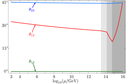
Figure 2: RG evolution of the mixing angles from the GUT scale to the SUSY-breaking scale (taken to be $\approx 1$ TeV) in the MSSM extended by heavy singlets for a normal mass hierarchy and $Y_{\nu}=X\,\operatorname{diag}\left(1,\varepsilon,\varepsilon^{2}\right)$ with $\tan\beta=5$, $\varepsilon=0.525$, $a=0.0675$ eV and $X=1$. In this example, the lightest neutrino has a mass of $0.025$ eV. The kinks in the plots correspond to the mass thresholds at the see-saw scales. The grey-shaded regions mark the various effective theories.

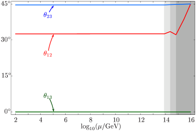
Figure 3: Example for the RG evolution of the mixing angles in the SM extended by heavy singlets from the GUT scale to the EW scale for a normal mass hierarchy and $Y_{\nu}=X\,\operatorname{diag}\left(1,\varepsilon,\varepsilon^{2}\right)$ with $\varepsilon=0.65$, $a=0.0655$ eV and $X=1$. In this example, the lightest neutrino has a mass of $0.024$ eV.

5 Analytic Approximation for the Running of the Mixing Angles at the GUT Scale

In order to understand the effect found numerically in the previous section, we now derive an analytic approximation for the RG evolution of the mixing angles at the GUT scale. It is only affected by the part of the RGE that is not proportional to the unit matrix, which is given by

$$16\pi^{2}\,\mu\frac{\mathrm{d}}{\mathrm{d}\mu}m_{\nu} = C_{e}\left[Y_{e}^{\dagger}Y_{e}\right]^{T}m_{\nu}+C_{e}\,m_{\nu}\left[Y_{e}^{\dagger}Y_{e}\right]$$ (10)

$${}+C_{\nu}\left[Y_{\nu}^{\dagger}Y_{\nu}\right]^{T}m_{\nu}+C_{\nu}\,m_{\nu}\left[Y_{\nu}^{\dagger}Y_{\nu}\right]$$

$${}+\;\mbox{terms with trivial flavour structure}$$

with $C_{e}=-\tfrac{3}{2}$, $C_{\nu}=\tfrac{1}{2}$ in the SM and $C_{e}=C_{\nu}=1$ in the MSSM. Analogously to equation (4), $m_{\nu}$ is parametrized by

$$m_{\nu}(t)=V\big{(}\theta_{12}(t),\theta_{13}(t),\theta_{23}(t)\big{)}\cdot m_{\mathrm{diag}}(t)\cdot V^{T}\big{(}\theta_{12}(t),\theta_{13}(t),\theta_{23}(t)\big{)}\;,$$ (11)

where $\mu$ is the renormalization scale, $t:=\ln\frac{\mu}{\mu_{0}}$, and $m_{\mathrm{diag}}:=\operatorname{diag}(m_{1},m_{2},m_{3})$. In general, the real $Y_{\nu}$ can be written as

$$Y_{\nu}=V(\xi_{12},\xi_{13},\xi_{32})\cdot\operatorname{diag}(y_{1},y_{2},y_{3})\cdot V^{T}(\phi_{12},\phi_{13},\phi_{32})\;.$$ (12)

However, the effective mixing matrix $m_{\nu}$ is invariant under the transformations $Y_{\nu}\rightarrow V^{T}Y_{\nu}$ and $M\rightarrow V^{T}MV$, which correspond to a change of basis for the heavy sterile neutrinos. Thus, $V(\xi_{12},\xi_{13},\xi_{32})$ in equation (12) can be absorbed into $M$, leading to the simpler parametrization

$$Y_{\nu}(y_{1},y_{2},y_{3},\phi_{12},\phi_{13},\phi_{32})=\operatorname{diag}(y_{1},y_{2},y_{3})\cdot V^{T}(\phi_{12},\phi_{13},\phi_{32})\;.$$ (13)

Furthermore, we use the approximation that the effect of the charged lepton Yukawa matrices $Y_{e}$ can be neglected compared to that of the neutrino Yukawa matrix. Note that in the MSSM a large $\tan\beta$ can yield a relatively large $Y_{e}$, which can also have sizable effects that are neglected in this approximation.

We now differentiate equation (11) w.r.t. $t$ and insert the RGE (10). For the evolution of the mixing angles at the GUT scale with bimaximal mixing as initial condition, we thus obtain both in the SM and in the MSSM the ratios

$$\left.\frac{\dot{\theta}_{12}}{\dot{\theta}_{13}}\right|_{M_{\mathrm{GUT}}} = \frac{2\,{\sqrt{2}}\,\left(m_{1}+m_{2}\right)\,\left(m_{3}-m_{1}\right)\,\left(m_{3}-m_{2}\right)\,\,F_{1}}{\left(m_{2}-m_{1}\right)\,\left[8\,\left(m_{3}^{2}-m_{1}\,m_{2}\right)\,F_{2}+4\,{\sqrt{2}}\,\left(m_{2}-m_{1}\right)\,m_{3}\,F_{3}\right]}$$ (14c)

$$\approx \left\{\begin{array}[]{ll}\displaystyle\pm\frac{1}{2\sqrt{2}}\,\frac{m_{2}+m_{1}}{m_{2}-m_{1}}\,\frac{F_{1}}{F_{2}}&\mbox{for hierarchical neutrino masses}\\[8.53581pt] \displaystyle\frac{1}{2\sqrt{2}}\,\frac{\Delta m_{\mathrm{atm}}^{2}}{\Delta m_{\mathrm{sol}}^{2}}\,\frac{F_{1}}{F_{2}}&\mbox{for degenerate neutrino masses}\end{array}\right.$$

$$\left.\frac{\dot{\theta}_{12}}{\dot{\theta}_{23}}\right|_{M_{\mathrm{GUT}}} = \frac{2\,{\sqrt{2}}\,\left(m_{1}+m_{2}\right)\,\left(m_{3}-m_{1}\right)\,\left(m_{3}-m_{2}\right)\,F_{1}}{\left(m_{2}-m_{1}\right)\,\left[8\,\left(m_{2}-m_{1}\right)\,m_{3}\,F_{2}+4\,{\sqrt{2}}\,\left(m_{3}^{2}-m_{1}\,m_{2}\right)F_{3}\right]}$$ (14f)

$$\approx \left\{\begin{array}[]{ll}\displaystyle\pm\frac{1}{2}\,\frac{m_{2}+m_{1}}{m_{2}-m_{1}}\,\frac{F_{1}}{F_{3}}&\mbox{for hierarchical neutrino masses}\\[8.53581pt] \displaystyle\frac{1}{2}\,\frac{\Delta m_{\mathrm{atm}}^{2}}{\Delta m_{\mathrm{sol}}^{2}}\,\frac{F_{1}}{F_{3}}&\mbox{for degenerate neutrino masses}\end{array}\right.$$

with

$$F_{1} = \left(y_{1}^{2}-y_{2}^{2}\right)\,\left\{\vphantom{y_{1}^{2}}\cos(2\,\phi_{12})\,\left[\vphantom{y_{1}^{2}}\left(\cos(2\,\phi_{13})-3\right)\,\sin(2\,\phi_{23})-6\,\cos^{2}(\phi_{13})\right]\right.$$

$${}\left.\hphantom{\left(y_{1}^{2}-y_{2}^{2}\right)\,\left\{\right.}-4\,\cos(2\,\phi_{23})\,\sin(2\,\phi_{12})\,\sin(\phi_{13})\vphantom{y_{1}^{2}}\right\}$$

$$+\left(y_{1}^{2}+y_{2}^{2}-2\,y_{3}^{2}\right)\,\left[\vphantom{y_{1}^{2}}\cos(2\,\phi_{13})\,\left(\sin(2\,\phi_{23})-3\right)+\left(1+\sin(2\,\phi_{23})\right)\vphantom{y_{1}^{2}}\right]\,,$$

$$F_{2} = 2\,\left(y_{1}^{2}-y_{2}^{2}\right)\,\cos(\phi_{13})\,\sin(2\,\phi_{12})\,\left(\sin(\phi_{23})-\cos(\phi_{23})\right)$$ (15b)

$$-\left(y_{1}^{2}+y_{2}^{2}-2\,{y_{3}}^{2}+\left(y_{1}^{2}-y_{2}^{2}\right)\,\cos(2\,\phi_{12})\right)\times$$

$${}\qquad\times\sin(2\,\phi_{13})\,\left(\cos(\phi_{23})+\sin(\phi_{23})\right)\;,$$

$$F_{3} = \left(y_{1}^{2}-y_{2}^{2}\right)\,\left[\vphantom{y_{1}^{2}}\cos(2\,\phi_{12})\,\left(\cos(2\,\phi_{13})-3\right)\,\cos(2\,\phi_{23})\right.$$ (15c)

$$\hphantom{\left(y_{1}^{2}-y_{2}^{2}\right)\,\left[\right.}\left.{}+4\,\sin(2\,\phi_{12})\,\sin(\phi_{13})\,\sin(2\,\phi_{23})\vphantom{y_{1}^{2}}\right]$$

$${}+2\,\left(y_{1}^{2}+y_{2}^{2}-2\,y_{3}^{2}\right)\,\cos^{2}(\phi_{13})\,\cos(2\,\phi_{23})\;.$$

This result can also be obtained from the formulae derived in [26]. The constants $F_{1}$, $F_{2}$ and $F_{3}$ clearly depend on the choice of $Y_{\nu}(M_{\mathrm{GUT}})$. However, unless the parameters $\{y_{1},y_{2},y_{3},\phi_{12},\phi_{13},\phi_{32}\}$ are fine-tuned, we expect the ratios $F_{1}/F_{2}$ and $F_{1}/F_{3}$ to be of the order one. Consequently, the RG change of $\theta_{12}$ is larger than that of the other angles if the mass-dependent factors in equations (14) are large. This is always the case for degenerate neutrino masses, since $\Delta m^{2}_{\mathrm{atm}}\gg\Delta m^{2}_{\mathrm{sol}}$. As $(m_{1}\!-\!m_{2})$ is related to the small solar mass squared difference, it is also true for non-degenerate mass schemes, unless $m_{1}$ is very small, in which case the ratio approaches 1. This corresponds to a normal mass hierarchy and a strongly hierarchical mass scheme. Finally, it can be shown that the running of $\theta_{12}$ is always enhanced compared to that of $\theta_{13}$ and $\theta_{23}$ for inverted schemes. Hence, we conclude that this is a generic effect.

6 Parameter Space Regions Compatible with the LMA Solution

6.1 Parameters at the GUT Scale

The considerable change of the solar mixing angle found in the previous sections raises the question whether the parameter region of the LMA solution might be reached by RG evolution, if one starts with bimaximal mixing at high energy. We will investigate this possibility by further numerical calculations in the following. To reduce the parameter space for the numerical analysis, we choose a specific neutrino Yukawa coupling $Y_{\nu}$ at the GUT scale. We assume that it is diagonal and of the form

$$Y_{\nu}=X\,\operatorname{diag}\left(1,\varepsilon,\varepsilon^{2}\right)\;.$$ (16)

$Y_{\nu}$ and $M$ are now determined by the parameters $\{\varepsilon,X,a,b,c\}$. Moreover, we fix the GUT scale values of $b$ and $c$ by the requirement that the solar and atmospheric mass squared differences obtained at the EW scale after the RG evolution be compatible with the allowed experimental regions. Thus, we are left with the free parameters $X$, $\varepsilon$ and $a$. The parameter $\varepsilon$ controls the hierarchy of the entries in $Y_{\nu}$ and thus the degeneracy of the see-saw scales, while $a$ determines the mass of the lightest neutrino. The dependence of physical quantities on $\varepsilon$ and $a$ is shown in figure 4. The effect of changing the scale $X$ of the neutrino Yukawa coupling will be discussed in section 6.3. As mentioned above, we work in the basis where the Yukawa matrix of the charged leptons is diagonal.

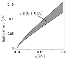
(a) Parameter $a$

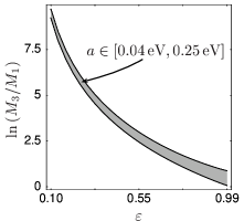
(b) Parameter $\varepsilon$

Figure 4: Plot 4(a) shows the mass of the lightest neutrino (at low energy) as a function of $a$ for the SM and the MSSM with normal mass hierarchy, $X=1$ and $\varepsilon\in[0.1,0.99]$ (grey region). Plot 4(b) shows the degeneracy of the see-saw scales, parametrized by $\ln(M_{3}/M_{1})$ (at the GUT scale), as a function of $\varepsilon$ for the same cases with $a\in[0.04\text{ eV},0.25\text{ eV}]$ (grey region).

6.2 Allowed Parameter Space Regions

The parameter space regions in which the RG evolution produces low-energy values compatible with the LMA solution are shown in figure 5 for the SM and the MSSM ($\tan\beta=5$) with a normal mass hierarchy. We find that for the form of $Y_{\nu}$ under consideration, hierarchical and degenerate neutrino mass schemes as well as degenerate and non-degenerate see-saw scales are possible. For inverted neutrino mass spectra, allowed parameter space regions exist as well.

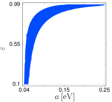
(a) SM

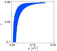
(b) MSSM

Figure 5: Parameter space regions compatible with the LMA solution of the solar neutrino problem for the example $Y_{\nu}=\operatorname{diag}(1,\varepsilon,\varepsilon^{2})$. The initial condition at the GUT scale $M_{\mathrm{GUT}}=10^{16}$ GeV is bimaximal mixing, and the comparison with the experimental data is performed at the EW scale or at 1 TeV for the SM and the MSSM, respectively. The white regions of the plots are excluded by the data (LMA) at $3\sigma$. For this example, we consider the case of a normal neutrino mass hierarchy and $X=1$ for the scale factor of the neutrino Yukawa couplings.

We would like to stress that the shape of the allowed parameter space regions strongly depends on the choice of the initial value of $Y_{\nu}$ at the GUT scale. One also has to ensure that the sign of $\Delta m^{2}_{\mathrm{sol}}$ is positive, as the LMA solution requires this if the convention is used that the solar mixing angle is smaller than $45^{\circ}$. With bimaximal mixing at the GUT scale, the sign of $\Delta m^{2}_{\mathrm{sol}}$ is not defined by the initial conditions. Using the analytic approximation of section 5, the sign just below the GUT scale can be calculated. We find $\Delta m^{2}_{\mathrm{sol}}>0$ for $F_{1}<0$ and vice versa. However, in order to predict the sign of $\Delta m^{2}_{\mathrm{sol}}$ at low energy, the numerical RG evolution has to be used. This excludes some of the possible choices for the neutrino Yukawa coupling $Y_{\nu}$ at the GUT scale. For example, among the possibilities with diagonal $Y_{\nu}$ it excludes $Y_{\nu}=\operatorname{diag}(\varepsilon^{2},\varepsilon,1)$.

6.3 Dependence on the Scale $X$ of the Neutrino Yukawa Coupling

For small values of $X$, the contribution from $Y_{\nu}$ to the evolution of the mixing angles above the largest see-saw scale is suppressed by a factor of $X^{2}$. Nevertheless, the evolution to the LMA solution is still possible, as can be seen from the example in figure 6. Here the large change of $\theta_{12}$ also seems to be generic but takes place between the see-saw scales, which shows the importance of carefully studying the RG behavior in these intermediate regions [20]. Note that in this case the analytic approximation of section 5 cannot be applied, since it is only valid at the GUT scale.

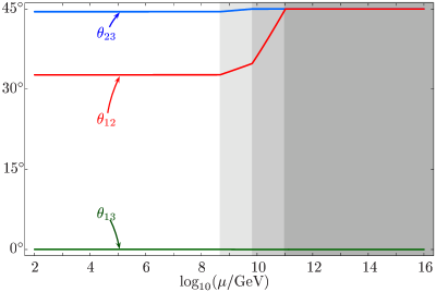
Figure 6: RG evolution in the SM for $X=0.01$, $\varepsilon=0.3$, $a=0.0535$ eV and a normal mass hierarchy. The running from bimaximal mixing to the LMA solution now takes place between the see-saw scales. In this example, the lightest neutrino has a mass of $0.017$ eV.

6.4 Effect of Neutrino CP Parities

An example for the running of the mixing angles to the LMA solution with a negative CP parity for the state with mass $m_{2}$ is shown in figure 7. For this we have chosen a different diagonal structure for $Y_{\nu}$,

$$Y_{\nu}=X\,\operatorname{diag}\left(\varepsilon^{2},\varepsilon,1\right)\;,$$ (17)

at the GUT scale. Here, the evolution to the LMA solution is possible due to running between the see-saw scales. A more detailed study of the effect of CP phases will be given in a forthcoming paper [27].

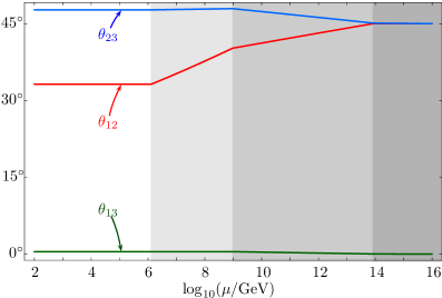
Figure 7: RG evolution in the SM with a negative CP parity for $m_{2}$, $X=0.5$, $\varepsilon=3.5\cdot 10^{-3}$ and a normal mass hierarchy. The running from bimaximal mixing to the LMA solution takes place between the see-saw scales. In this example, we consider a strongly hierarchical mass spectrum. The lightest neutrino has a mass of $0.004$ eV. Note that the cases $\theta_{23}>45^{\circ}$, $\Delta m^{2}_{23}>0$ and $\widetilde{\theta}_{23}:=90^{\circ}-\theta_{23}<45^{\circ}$, $\Delta\widetilde{m}^{2}_{23}:=-\Delta m^{2}_{23}$ are indistinguishable in neutrino oscillations.

The large RG effects in this case seem surprising at first sight, since previous studies, e.g. [18, 26], found that opposite CP parities for $m_{1}$ and $m_{2}$ prevent a sizable change of the solar mixing angle by RG evolution. However, these works did not consider the energy region between the see-saw scales, where the largest change occurs in our example. This fact explains the apparent discrepancy.

6.5 Low Scale Values of $\theta_{13}$ and $\theta_{23}$

The mixing angles $\theta_{13}$ and $\theta_{23}$ are affected by the RG evolution as well, i.e. they do not stay at their initial values $\theta_{13}=0^{\circ}$ and $\theta_{23}=45^{\circ}$. However, lower bounds on their changes cannot be given unless a specific model is chosen. As one can see from the previous examples, the changes can be tiny. For instance, the evolution of figure 2 gives $\Delta\theta_{13}=0.02^{\circ}$, which corresponds to $\sin^{2}(2\theta_{13})=5\cdot 10^{-7}$, and $\Delta\theta_{23}=0.28^{\circ}$. On the other hand, other choices of $Y_{\nu}$ at the GUT scale produce $\Delta\theta_{13}$ and $\Delta\theta_{23}$ that come close to the experimental bounds. This can make it possible to discriminate between models with different initial values $Y_{\nu}(M_{\mathrm{GUT}})$.

7 Summary and Conclusions

We have shown that in see-saw scenarios the experimentally favored neutrino mass parameters with the LMA solution of the solar neutrino problem can be obtained in a rather generic way from bimaximal mixing at the GUT scale by Renormalization Group running. We have concentrated on the case of vanishing CP phases, which implies positive mass eigenvalues. In an example where the mass eigenstates corresponding to the solar mass squared difference have opposite CP parity, we have demonstrated that an evolution towards the LMA solution is possible in this case as well. The general case of arbitrary CP phases is beyond the scope of this letter and will be studied elsewhere [27]. The mixing angles evolved down to the electroweak scale show a strong dependence on the mass scale of the lightest neutrino, on the degeneracy of the see-saw scales, and on the form of the neutrino Yukawa coupling. A generic feature of the Renormalization Group evolution is that the solar mixing angle $\theta_{12}$ evolves towards sizably smaller values, whereas the change of $\theta_{13}$ and $\theta_{23}$ is comparatively small. In the SM and MSSM, we find extensive regions in parameter space which are compatible with the LMA solution for normal and inverted neutrino mass hierarchies and for large and small absolute scales of the neutrino Yukawa couplings. Thus, RG running may provide a natural explanation for the observed deviation of the LMA mixing angles from bimaximality.

References

- [1] V. Barger, D. Marfatia, K. Whisnant, and B. P. Wood, Imprint of SNO neutral current data on the solar neutrino problem, Phys. Lett. B537 (2002), 179–186 (hep-ph/0204253).
- [2] A. Bandyopadhyay, S. Choubey, S. Goswami and D. P. Roy, Implications of the first neutral current data from SNO for solar neutrino oscillation, hep-ph/0204286.
- [3] J. N. Bahcall, M. C. Gonzalez-Garcia and C. Peña-Garay, Before and After: How has the SNO NC measurement changed things?, hep-ph/0204314.
- [4] P. C. de Holanda and A. Yu. Smirnov, Solar neutrinos: Global analysis with day and night spectra from SNO, hep-ph/0205241.
- [5] T. Toshito et al. [Super-Kamiokande Collaboration], Super-Kamiokande atmospheric neutrino results, hep-ex/0105023.
- [6] M. Apollonio et al. [CHOOZ Collaboration], Limits on neutrino oscillations from the CHOOZ experiment, Phys. Lett. B466 (1999), 415 (hep-ex/9907037).
- [7] M. Tanimoto, Renormalization effect on large neutrino flavor mixing in the minimal supersymmetric standard model, Phys. Lett. B360 (1995), 41–46 (hep-ph/9508247).
- [8] K. R. S. Balaji, A. S. Dighe, R. N. Mohapatra and M. K. Parida, Radiative magnification of neutrino mixings and a natural explanation of the neutrino anomalies, Phys. Lett. B481 (2000), 33–38 (hep-ph/0002177).
- [9] T. Miura, E. Takasugi and M. Yoshimura, Quantum effects for the neutrino mixing matrix in the democratic-type model, Prog. Theor. Phys. 104 (2000), 1173–1187 (hep-ph/0007066).
- [10] G. Dutta, Stable bimaximal neutrino mixing pattern, hep-ph/0203222.
- [11] J. R. Ellis and S. Lola, Can neutrinos be degenerate in mass?, Phys. Lett. B458 (1999), 310–321 (hep-ph/9904279).
- [12] J. A. Casas, J. R. Espinosa, A. Ibarra and I. Navarro, Naturalness of nearly degenerate neutrinos, Nucl. Phys. B556 (1999), 3–22 (hep-ph/9904395).
- [13] J. A. Casas, J. R. Espinosa, A. Ibarra and I. Navarro, Nearly degenerate neutrinos, supersymmetry and radiative corrections, Nucl. Phys. B569 (2000), 82–106 (hep-ph/9905381).
- [14] P. H. Chankowski, A. Ioannisian, S. Pokorski and J. W. F. Valle, Neutrino unification, Phys. Rev. Lett. 86 (2001), 3488–3491 (hep-ph/0011150).
- [15] M.-C. Chen and K. T. Mahanthappa, Implications of the renormalization group equations in three neutrino models with two-fold degeneracy, Int. J. Mod. Phys. A16 (2001), 3923–3930 (hep-ph/0102215).
- [16] M. K. Parida, C. R. Das and G. Rajasekaran, Radiative stability of neutrino-mass textures, hep-ph/0203097.
- [17] P. H. Chankowski, W. Krolikowski and S. Pokorski, Fixed points in the evolution of neutrino mixings, Phys. Lett. B473 (2000), 109 (hep-ph/9910231).
- [18] N. Haba, Y. Matsui and N. Okamura, The effects of majorana phases in three-generation neutrinos, Eur. Phys. J. C17 (2000), 513–520 (hep-ph/0005075).
- [19] S. F. King and N. N. Singh, Renormalisation group analysis of single right-handed neutrino dominance, Nucl. Phys. B591 (2000), 3–25 (hep-ph/0006229).
- [20] S. Antusch, J. Kersten, M. Lindner and M. Ratz, Neutrino mass matrix running for non-degenerate see-saw scales, Phys. Lett. B538 (2002), 87–95 (hep-ph/0203233).
- [21] P. H. Chankowski and Z. Pluciennik, Renormalization group equations for seesaw neutrino masses, Phys. Lett. B316 (1993), 312 (hep-ph/9306333).
- [22] K. S. Babu, C. N. Leung and J. Pantaleone, Renormalization of the neutrino mass operator, Phys. Lett. B319 (1993), 191 (hep-ph/9309223).
- [23] S. Antusch, M. Drees, J. Kersten, M. Lindner and M. Ratz, Neutrino mass operator renormalization revisited, Phys. Lett. B519 (2001), 238–242 (hep-ph/0108005).
- [24] S. Antusch, M. Drees, J. Kersten, M. Lindner and M. Ratz, Neutrino mass operator renormalization in two Higgs doublet models and the MSSM, Phys. Lett. B525 (2002), 130 (hep-ph/0110366).
- [25] S. Antusch and M. Ratz, Supergraph techniques and two-loop beta-functions for renormalizable and non-renormalizable operators, hep-ph/0203027.
- [26] J. A. Casas, J. R. Espinosa, A. Ibarra and I. Navarro, General RG equations for physical neutrino parameters and their phenomenological implications, Nucl. Phys. B573 (2000), 652 (hep-ph/9910420).
- [27] S. Antusch, J. Kersten, M. Lindner and M. Ratz, In preparation.