INCLUSIVE HIGGS BOSON PRODUCTION AT HADRON COLLIDERS AT NEXT-TO-NEXT-TO-LEADING ORDER

Inclusive production via gluon fusion will be the most important production channel for Higgs boson discovery at the LHC. I report on a calculation of the inclusive Higgs boson production cross section at $pp$ and $p\bar{p}$ colliders at next-to-next-to-leading order in QCD.

1 Introduction

The Standard Model is almost thirty-five years old, and its basic assertion, that the weak and electromagnetic interactions unify in a spontaneously broken $SU(2)_{L}\otimes U(1)_{Y}$ gauge theory has been spectacularly confirmed at the quantum level by the precision experiments at LEP and the SLC. Still, the crucial ingredient, the agent of electroweak symmetry breaking, remains a mystery.

The benchmark for studies of the symmetry breaking sector is the minimal standard model, in which a single complex scalar doublet is introduced. Upon, spontaneous symmetry breakdown, a single Higgs boson is left as the signature of the symmetry breaking sector. The final run at LEP established a 95% confidence-level lower limit for the Higgs boson of $114.1$ GeV $\!{}^{{\bf?}}$. The Higgs boson can also be constrained by its effect on precisely measured electroweak observables. The current best fit produced by the LEP Electroweak Working Group predicts that $M_{H}=85^{+54}_{-34}$ GeV, with a 95% confidence-level upper limit of $M_{H}<196$ GeV.

With the end of LEP, the search for the Higgs boson is left to hadron colliders, the Fermilab Tevatron and the CERN LHC. Higgs production at hadron colliders is dominated by the gluon fusion mechanism, where gluons excite virtual top quark loops which couple strongly to the Higgs. Despite its dominance, this production process cannot be exploited at the Tevatron unless the Higgs boson mass is near the $WW$ threshold. For lighter Higgs masses, the dominant decay mode, $H\to b\bar{b}$ is overwhelmed by the QCD background and the overall rate is too low to permit the use of rare decay modes. Therefore, the Tevatron experiments must primarily rely on the associated production mechanism, $q\bar{q}\to H+W$, for their Higgs search.

At the LHC, however, gluon fusion is the most important production mechanism for Higgs discovery for masses below $\sim 700$ GeV, since the rate will be sufficiently high that one can use the rare decay mode $H\to\gamma\gamma$ in the low mass region. The discovery of the Higgs boson and the subsequent study of its properties therefore relies on a solid theoretical understanding of the gluon fusion production mechanism.

Unfortunately, next-to-leading order (NLO) studies $\!{}^{{\bf?},{\bf?}}$ of inclusive Higgs production do not provide this solid understanding. The NLO corrections are very large, of order $70-100$%, and initial estimates of next-to-next-to-leading order (NNLO) corrections $\!{}^{{\bf?}}$ based on soft plus collinear resummation indicated that they too might be very large. The unsettled nature of such an important signal clearly calls for a renewed effort to bring this process under control.

Last year, two groups presented calculations of the soft plus virtual contributions to the NNLO correction $\!{}^{{\bf?},{\bf?}}$. It was known from NLO corrections that soft plus virtual terms alone significantly underestimate the full correction. The leading hard scattering term is completely collinear in nature and can be reliably obtained from resummation. The combined soft plus virtual plus collinear (SVC) approximation $\!{}^{{\bf?}}$ predicts that the total NNLO correction will be much more moderate than the initial estimate $\!{}^{{\bf?}}$. Still, one would like a full NNLO calculation to verify that inclusive Higgs boson production is under perturbative control. In this talk, I will present the results of that calculation $\!{}^{{\bf?}}$.

2 The Calculation

In the limit that all quark masses except that of the top quark vanish, gluons couple to Higgs only via top quark loops. This coupling can be approximated by an effective Lagrangian $\!{}^{{\bf?}}$ corresponding to the limit $m_{t}\to\infty$, which is valid for a large range of $M_{H}$, including the currently favored region between 100 and 200 GeV. The effective Lagrangian is

$${\cal L}_{\rm eff}=-\frac{H}{4v}C_{1}(\alpha_{s})\,G_{\mu\nu}^{a}G^{a\,\mu\nu}\,,$$ (1)

where $G_{\mu\nu}^{a}$ is the gluon field strength tensor, $H$ is the Higgs field, $v\approx 246$ GeV is the vacuum expectation value of the Higgs field and $C_{1}(\alpha_{s})$ is the Wilson coefficient, which for this calculation we need to order $(\alpha_{s}^{3})$ $\!{}^{{\bf?},{\bf?}}$.

Three classes of Feynman diagrams must be evaluated to compute the NNLO cross section: (i) two-loop virtual diagrams for $gg\to H$; (ii) one-loop single real emission diagrams for $gg\to Hg$, $gq\to Hq$, and $q\bar{q}\to Hg$; (iii) tree-level double real emission diagrams for $gg\to Hgg$, $gg\to Hq\bar{q}$, $gq\to Hgq$, $qq\to Hqq$, $q\bar{q}\to Hgg$, and $q\bar{q}\to Hq\bar{q}$. Sample diagrams are shown in Figure 1.

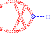
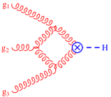
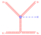
(a) (b) (c) (d)

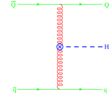
Figure 1: Sample diagrams of (a) virtual (b) single real emission and (c,d) double real emission corrections.

The most difficult part of the calculation, by far, is the computation of the corrections due to double real emission. While the (tree-level) matrix elements are quite easy to compute, the integration over double-emission phase space is quite complicated. We find, however, that if we expand the double real emission integrals as power series about soft limit (where the partonic center-of-mass energy is close to the Higgs mass, $M_{H}^{2}/\hat{s}\equiv x\to 1$), the integrals simplify dramatically. Moreover, the series expansion is well-behaved and converges quite rapidly.

Thus, while we have computed the virtual corrections, single real emission and the effects of mass factorization in closed analytic form, we have computed double real emission in the form of a power series. The closed-form results can also be readily expressed as power series, so we present the full partonic cross section as an expansion in $(1-x)$ and $\ln(1-x)$:

$$\begin{split}\hat{\sigma}_{ij}&=\sum_{n\geq 0}\left(\frac{\alpha_{s}}{\pi}\right)^{n}\,\hat{\sigma}_{ij}^{(n)}\,,\\ \hat{\sigma}_{ij}^{(n)}&=a^{(n)}\,\delta(1-x)+\sum_{k=0}^{2n-1}b_{k}^{(n)}\left[\frac{\ln^{k}(1-x)}{1-x}\right]_{+}+\sum_{l=0}^{\infty}\sum_{k=0}^{2n-1}c_{lk}^{(n)}\,(1-x)^{l}\ln^{k}(1-x)\,,\\ x&=\frac{M_{H}^{2}}{\hat{s}}\,.\end{split}$$ (2)

Note that if all coefficients are computed, this is an exact expression for the partonic cross section. In practice, we compute only a finite number of terms. The soft plus virtual approximation includes only the $a^{(2)}$ and $b^{(2)}_{k}$ terms at second order. The SVC approximation also includes the $c^{(2)}_{03}$ coefficient. We have now computed all coefficients $c^{(2)}_{lk}$ through $l=16$ $\!{}^{{\bf?}}$. As can be seen in Figure 3, this is more than enough terms to obtain a reliable result for the total cross section.

In Figure 2(a), we show the cross section at LO, NLO and NNLO. At each order, we use the corresponding MRST parton distribution set $\!{}^{{\bf?}}$.

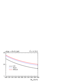
(a) (b)

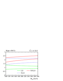
Figure 2: (a) LO (dotted), NLO (dashed) and NNLO (solid) cross sections for Higgs production at the LHC ($\mu_{F}=\mu_{R}=M_{H}$). In each case, we weight the cross section by the ratio of the LO cross section in the full theory ($M_{t}=175$ GeV) to the LO cross section in the effective theory (Eq. (1)).(b) Scale dependence at the LHC. The lower curve of each pair corresponds to $\mu_{R}=2M_{H}$, $\mu_{F}=M_{H}/2$, the upper to $\mu_{R}=M_{H}/2$, $\mu_{F}=2M_{H}$. The $K$-factor is computed with respect to the LO cross section at $\mu_{R}=\mu_{F}=M_{H}$.

One immediately sees that the true NNLO correction, while substantial, is much smaller than the NLO correction. Indeed, it is even a bit smaller than predicted by the SVC approximation. Nonetheless, it verifies that the SVC is a good approximation of the total cross section.

Figure 2(b) shows the renormalization and factorization scale dependence of the “K factor”, the ratio of the NLO and NNLO cross sections to the leading order cross section. The scale dependence of the NNLO cross section is still quite large, though somewhat smaller than at NLO.

Figure 3 shows the rapid convergence of the power series expansion in $(1-x)$. Observe that the purely soft contributions underestimate the cross section by $\sim 10\%-15\%$, while the next term, $\propto(1-x)^{0}$, overestimates it by about $5\%$. By the time the third term in the series is included ($\propto(1-x)^{1}$), one is within $1\%$ of the result obtained by computing the first 18 terms (through $(1-x)^{16}$). In light of the large scale uncertainty in the result, there is little or no precision to be gained from computing higher order terms in the expansion.

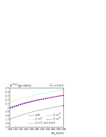
Figure 3: $K$-factor for Higgs production at the LHC. Each line corresponds to a different order in the expansion in $(1-x)$. The renormalization and factorization scales are set to $M_{H}$.

In conclusion, we have computed the full NNLO corrections to inclusive Higgs boson production at hadron colliders. We find reasonable perturbative convergence and reduced scale dependence.

References

References

- [1] U. Schwickerath, these proceedings, hep-ph/0205126.
-
[2]
S. Dawson, Nucl. Phys. B 359, 283 (1991);
A. Djouadi et al, Phys. Lett. B 264, 440 (1991). -
[3]
D. Graudenz et al, Phys. Rev. Lett. 70, 1372 (1993);
M. Spira et al, Nucl. Phys. B 453, 17 (1995). - [4] M. Krämer et al., Nucl. Phys. B 511, 523 (1998).
- [5] R.V. Harlander and W.B. Kilgore, Phys. Rev. D 64, 013015 (2001).
- [6] S. Catani et al, J. High Energy Phys. 05, 25 (2001).
- [7] R.V. Harlander and W.B. Kilgore, Phys. Rev. Lett. 88, 201801 (2002).
-
[8]
A. Vainshtein et al., Yad. Fiz. 30, 1368 (1979)
[Sov. J. Nucl. Phys. 30, 1979 (711)];
A. Vainshtein et al., Usp. Fiz. Nauk 146, 683 (1985) [Sov. Phys. Usp. 23, 1980 (429)];
M. Voloshin, Yad. Fiz. 44, 738 (1986) [Sov. J. Nucl. Phys. 44, 478 (1986)]. - [9] K.G. Chetyrkin et al., Phys. Rev. Lett. 79, 353 (1997); Nucl. Phys. B 510, 61 (1998).
- [10] A.D. Martin et al., Eur. Phys. J. C 23, 73 (2002); Phys. Lett. B 531, 216 (2002).