NSF-ITP-02-40
                                                                 ITP, UCSB, Santa Barbara
Gluon Shadowing in Heavy Flavor Production off Nuclei

Abstract

Gluon shadowing which is the main source of nuclear effects for production of heavy flavored hadrons, remains unknown. We develop a light-cone dipole approach aiming at simplifying the calculations of nuclear shadowing for heavy flavor production, as well as the cross section which does not need next-to-leading and higher order corrections. A substantial process dependence of gluon shadowing is found at the scale of charm mass manifesting a deviation from QCD factorization. The magnitude of the shadowing effect correlates with the symmetry properties and color state of the produced $\bar{c}c$ pair. It is about twice as large as in DIS [17], but smaller than for charmonium production [6]. The higher twist shadowing correction related to a nonzero size of the $\bar{c}c$ pair is not negligible and steeply rises with energy. We predict an appreciable suppression by shadowing for charm production in heavy ion collisions at RHIC and a stronger effect at LHC. At the same time, we expect no visible difference between nuclear effects for minimal bias and central collisions, as is suggested by recent data from the PHENIX experiment [41]. We also demonstrate that at medium high energies when no shadowing is possible, final state interaction may cause a rather strong absorption of heavy flavored hadrons produced at large $x_{F}$.

1 Introduction

It is still unclear whether available data from fixed target experiments demonstrate any nuclear effects for open charm production [1, 2, 3]. Naively one might expect no effects at all, since a heavy quark should escape the nucleus without attenuation or reduction of its momentum. In fact, this is not correct even at low energies as is explained below. Moreover, at high energies one cannot specify any more initial or final state interactions. The process of heavy flavor production takes a time interval longer than the nuclear size, and the heavy quarks are produced coherently by many nucleons which compete with each other. As a result the cross section is reduced, and this phenomenon is called shadowing.

In terms of parton model the same effect is interpreted in the infinite momentum frame of the nucleus as reduction of the nuclear parton density due to overlap and fusion of partons at small Bjorken $x$. The kinematic condition for overlap is the same as for coherence in the nuclear rest frame.

There are well known examples of shadowing observed in hard reactions, like deep-inelastic scattering (DIS) [4] and Drell-Yan process (DY) [5] demonstrating a sizeable reduction of the density of light sea quarks in nuclei. Shadowing is expected also for gluons, although there is still no experimental evidence for that.

Shadowing for heavy quarks is a higher twist effect, and although its magnitude is unknown within the standard parton model approach, usually it is neglected for charm and beauty production. However, this correction is proportional to the gluon density in the proton and steeply rises with energy. Unavoidably, such a correction should become large at high energies. In some instances, like for charmonium production, this higher twist effect gains a large numerical factor and leads to a rather strong suppression even at energies of fixed target experiments [6].

On the other hand, gluon shadowing which is the leading twist effect, is expected to be the main source of nuclear suppression for heavy flavor production at high energies. This is why this process is usually considered as a sensitive probe for the gluon density in hadrons and nuclei. If to neglect the power, $1/m_{Q}^{2}$, corrections (unless otherwise specified), then the cross section of heavy $\bar{Q}Q$ production in $pA$ collision is suppressed by the gluon shadowing factor $R^{G}_{A}$ compared to the sum of $A$ nucleon cross sections,

$$\sigma^{\bar{Q}Q}_{pA}(x_{1},x_{2})=R^{G}_{A}(x_{1},x_{2})\,A\,\sigma^{\bar{Q}Q}_{pN}(x_{1},x_{2})\ .$$ (1)

Here

$$R^{G}_{A}(x_{1},x_{2})={1\over A}\int d^{2}b\,R^{G}_{A}(x_{1},x_{2},b)\,T_{A}(b)\ ,$$ (2)

where $R^{G}_{A}(x_{1},x_{2},b)$ is the (dimensional) gluon shadowing factor at impact parameter $b$; $T_{A}(b)=\int_{-\infty}^{\infty}\,dz\,\rho_{A}(b,z)$ is the nuclear thickness function at impact parameter $b$; $x_{1},\ x_{2}$ are the Bjorken variables of the gluons participating in $\bar{Q}Q$ production from the colliding proton and nucleus.

Parton model cannot predict shadowing, but only its evolution at high $Q^{2}$, while the main contribution originates from the soft part of the interaction. The usual approach is to fit data at different values of $x$ and $Q^{2}$ employing the DGLAP evolution and fitting the distributions of different parton species parametrized at some intermediate scale [7, 8]. However, the present accuracy of data for DIS on nuclei do not allow to fix the magnitude of gluon shadowing, which is found to be compatible with zero . Nevertheless, the data exclude some models with too strong gluon shadowing [9].

Another problem faced by the parton model is impossibility to predict gluon shadowing effect in nucleus-nucleus collisions even if the shadowing factor Eq. (1) in each of the two nuclei was known. Indeed, the cross section of $\bar{Q}Q$ production in collision of nuclei $A$ and $B$ at impact parameter $\vec{b}$ reads,

$$\frac{d\sigma^{\bar{Q}Q}_{AB}(x_{1},x_{2})}{d^{2}b}=R^{G}_{AB}(x_{1},x_{2},b)\,AB\,\sigma^{\bar{Q}Q}_{NN}(x_{1},x_{2})\ ,$$ (3)

where

$$R_{AB}^{G}(x_{1},x_{2},b)=\frac{1}{AB}\int d^{2}s\,R^{G}_{A}(x_{1},\vec{s})\,T_{A}(s)\ R^{G}_{B}(x_{2},\vec{b}-\vec{s})\,T_{B}(\vec{b}-\vec{s})\ .$$ (4)

In order to calculate the nuclear suppression factor Eq. (4) one needs to know the impact parameter dependence of gluon shadowing, $R^{G}_{A}(x_{1},\vec{b})$, while only integrated nuclear shadowing Eq. (2) can be extracted from lepton- or hadron-nucleus data. Note that parton model prediction of shadowing effects for minimum bias events integrated over $b$ suffers the same problem. Apparently, QCD factorization cannot be applied to heavy ion collisions even at large scale. The same is true for quark shadowing expected for Drell-Yan process in heavy ion collisions [10, 11, 12].

Nuclear shadowing can be predicted within the light-cone (LC) dipole approach which describes it via simple eikonalization of the dipole cross section. It was pointed out in [13] that quark configurations (dipoles) with fixed transverse separations are the eigenstates of interaction in QCD, therefore eikonalization is an exact procedure. In this way one effectively sums up the Gribov’s inelastic corrections in all orders [13].

The advantage of this formalism is that it does not need any $K$-factor, since effectively includes all higher twist and next-to-leading, next-to-next… corrections. Of course, one assumes universality of the dipole cross section, i.e. its process independence. This property can be proven in the leading $\log(1/x)$ approximation, otherwise is an assumption of the model. Indeed, it was demonstrated recently in [14] that the simple dipole formalism for Drell-Yan process [10, 15, 16] precisely reproduces the results of very complicated next-to-leading calculations at small $x$. The LC dipole approach also allows to keep under control deviations from QCD factorization. In particular, we found a substantial process-dependence of gluon shadowing due to existence of a semi-hard scale imposed by the strong nonperturbative interaction of light-cone gluons [17]. For instance gluon shadowing for charmonium production off nuclei was found in [6] to be much stronger than in deep-inelastic scattering [17].

The LC dipole approach also provides effective tools for calculation of transverse momentum distribution of heavy quarks, like it was done for radiated gluons in [16, 18], or Drell-Yan pairs in [11]. Nuclear broadening of transverse momenta of the heavy quarks also is an effective way to access the nuclear modification of the transverse momentum distribution of gluons, so called phenomenon of color glass condensate or gluon saturation [19, 20]. In this paper we consider only integrated quantities and leave the transverse momentum distribution for further calculations.

In what follows we find sizeable deviations from QCD factorization for heavy quark production off nuclei. First of all, for open charm production shadowing related to propagation of a $\bar{c}c$ pair through a nucleus is not negligible, especially at the high energies of RHIC and LHC, in spite of smallness of $\bar{c}c$ dipoles. Further, higher Fock components containing gluons lead to gluon shadowing which also deviates from factorization and depends on quantum numbers of the produced heavy pair $\bar{c}c$.

This paper is organized as follows. In Sect. 2.1 we consider the contribution of the lowest Fock component $\bar{c}c$ of projectile gluons to production of a $\bar{c}c$ pair in $NN$ collisions. A LC representation is derived for three production amplitudes which are classified in accordance with the color and symmetry properties of the $\bar{c}c$. We are focusing on charm for the sake of concreteness, but all the results of the paper are applicable to production of beauty.

Multiple color-exchange interaction of a $\bar{c}c$ pair propagating through a nucleus are considered in Sect. 2.2. The corresponding nuclear shadowing has a form of the conventional Glauber eikonal, where the exponent contains the dipole cross section $\sigma_{3}$ of interaction of a 3-parton system $\bar{c}cG$.

Sect. 3 is devoted to the problem of gluon shadowing. First of all, a dipole representation for the process $GN\to\bar{c}c\,G\,X$ is derived in Sect. 3.1 and Appendix A. Three types of amplitudes are found, one for production of a colorless $\bar{c}c$ and a gluon, and two for color-octet $\bar{c}c$ and a gluon, corresponding to two possible symmetries of an octet-octet state.

The same reaction of gluon radiation accompanying $\bar{c}c$ pair production off nuclei is related to the phenomenon of gluon shadowing. It is described in Sect. 3.2 employing the technique of light-cone Green functions corresponding to propagation of a $\bar{c}cG$ system through nuclear matter.

Light-cone gluons are known to have a short range propagation radius in the transverse plane which we describe via a nonperturbative light-cone potential in the Schrödinger two-dimensional equation for the Green function. The strength of the potential depends on the color state and symmetry of the $\bar{c}cG$ system. Correspondingly, the LC nonperturbative wave functions are also different. In Sect. 3.3 we find three types of LC wave functions with different mean separations.

Naturally, gluon shadowing correlates with the size of the $\bar{c}cG$, therefore it demonstrates a strong process dependence, i.e. deviation from QCD factorization. Different types of gluon shadowing calculated in Sect. 3.4 are presented in Fig. 4. Since about $20\%$ of $\bar{c}c$ pair are produced in a colorless state, it is important to know the fraction of such pairs which end up in an open charm channel. This estimate is done in Sect, 3.5.

The results of these calculations are used in Sect. 4 to predict nuclear shadowing for open charm production in proton-nucleus collisions. This includes gluon as well as charm quark shadowing, and also possible medium modifications like EMC effect and gluon antishadowing. We provide predictions of nuclear effects plotted in Fig. 5 for open charm production in $p-W$ collisions at the energy of the HERA-B experiment.

In the same Sect. 4 we provide predictions for shadowing for charm production in heavy ion collisions at the energies of RHIC ($\sqrt{s}=200\,\mbox{GeV}$) and LHC ($\sqrt{s}=5500\,\mbox{GeV}$) depicted in Figs. 6 – 7. We found quite a sizeable contribution from the higher twist effect of shadowing related to size of the $\bar{c}c$ pair. A most interesting observation is nearly identical shadowing effects predicted for minimal bias and central collisions, what has been indeed observed recently by the PHENIX experiment at RHIC. We identify the source of such a coincidence, and emphasize that this observation should not be interpreted as an indication for weak nuclear effects. Indeed, Figs. 7 demonstrate a substantial nuclear shadowing even for RHIC.

In Sect. 5 we consider the case of medium high energies when noshadowing is possible since the coherence length is short. Then the $\bar{c}c$ pair is produced momentarily on a bound nucleon and then undergoes final state interactions. On the contrary to wide spread believe, we argue that these interactions lead to absorption related to an unusual configuration in which the heavy flavored hadron is created.

We summarize the results of calculations and observations in the concluding Sect. 6.

2 Light-cone dipole formalism for charm production

2.1 $NN$ collisions

For the sake of concreteness in what follows we consider charm $\bar{c}c$ pair production, unless otherwise specified. Our results are easily generalized to the case of heavier quarks. The parton model treats this process in the rest frame of the produced pair as glue-glue fusion, $GG\to\bar{c}c$. At the same time, in the rest frame of the nucleus it looks like interaction of a $\bar{c}c$ fluctuation which has emerged from a projectile gluon. Thus, the problem is reduced to the process,

$$G+N\to\bar{c}c+X\ .$$ (5)

In the LC dipole approach the cross section is represented by a sum over different Fock components of the projectile gluon whose LC wave functions squared are convoluted with proper dipole cross sections. The cross section corresponding to Feynman graphs depicted in Fig. 1 was calculated in [21] and it was found that it needs a dipole cross section corresponding to a three-body system $G\bar{c}c$.

Figure 1: Perturbative QCD mechanism of charm production production in a gluon-nucleon collision. Only the lowest $\bar{c}c$ Fock component of the gluon is taken into account.

This observation follows the general prescription [10] that the partonic process $a\to bc$ is related to the dipole cross section $\sigma_{\bar{a}bc}(\vec{r},\alpha)$ for the three-partonic $\bar{a}bc$ system with transverse separations $\vec{r}$ (for the $bc$), $\alpha\vec{r}$ ($\bar{a}c$) and $\bar{\alpha}\vec{r}$ ($b\bar{a}$). Here $\alpha$ and $\bar{\alpha}=1-\alpha$ are the fractions of the light-cone momentum of the parton $a$ carried by the partons $b$ and $c$ respectively (the notation used further on). The intuitive motivation for this prescription is rather transparent. The incident constituent parton $a$ contains different Fock components, the bare parton $|a\rangle$, the excitation $|bc\rangle$, etc. If the states $|a\rangle$ and $|bc\rangle$ had the same interaction amplitudes, no production process $a\to bc$ would be possible, since the composition of the coherent Fock components which build up the constituent parton $a$ remained unchanged. Thus, the production amplitude of $a\to bc$ is proportional to the difference of the interaction amplitudes $f_{a}-f_{(bc)}$ which coincides with the scattering amplitude $f_{(\bar{a}bc)}$. Remarkably, each of the amplitudes $f_{a}$ and $f_{(bc)}$ might be infra-red divergent (like in the case of $G\to\bar{c}c$), while $f_{(\bar{a}bc)}$ is infra-red stable due to color neutrality of the system.

Treating the process Eq. (5) in more detail, one should discriminate between three different color and spin states in which the $\bar{c}c$ pair can be produced. These states are orthogonal and do not interfere in the cross section. They include:

1. The color-singlet $C$-even $\bar{c}c$ state. The corresponding amplitude is odd (O) relative to simultaneous permutation of spatial and spin variables of the $\bar{c}c$ and has the form,

   $$A^{\bar{\mu}\mu}_{ij,a}(\vec{\kappa},\vec{k}_{T},\alpha)=\sum\limits_{e=1}^{8}{1\over 6}\,\delta_{ae}\,\delta_{ij}\ O^{\bar{\mu}\mu}_{e}(\vec{\kappa},\vec{k}_{T},\alpha)\ .$$ (6)

   Here $\vec{\kappa}$ and $\vec{k}_{T}$ are the relative and total transverse momenta of the $\bar{c}c$ pair respectively; $\mu,\bar{\mu}$ are spin indexes, $a$ and $i,j$ are color indexes of the gluon and produced quarks, respectively. We will classify such a state as $1^{-}$, which means a color singlet with odd parity relative to index permutation. Note the $1^{+}$ cannot be produced in the reaction Eq. (5).

2. Color-octet $\bar{c}c$ state with the production amplitude also antisymmetric relative simultaneous permutation of spatial and spin variables of the $\bar{c}c$ ($8^{-}$),

   $$B^{\bar{\mu}\mu}_{ij,a}(\vec{\kappa},\vec{k}_{T},\alpha)=\sum\limits_{e,g=1}^{8}{1\over 2}\,d_{aeg}\,\tau_{g}(ij)\ O^{\bar{\mu}\mu}_{e}(\vec{\kappa},\vec{k}_{T},\alpha)\ .$$ (7)

   Here $\lambda_{g}=\tau_{g}/2$ are the Gell-Mann matrixes.

3. Color-octet $\bar{c}c$ with the amplitude symmetric relative permutation of quark variables ($8^{+}$),

   $$C^{\bar{\mu}\mu}_{ij,a}(\vec{\kappa},\vec{k}_{T},\alpha)=\sum\limits_{e,g=1}^{8}{i\over 2}\,f_{aeg}\,\tau_{g}(ij)\ E^{\bar{\mu}\mu}_{e}(\vec{\kappa},\vec{k}_{T},\alpha)\ .$$ (8)

The amplitudes Eq. (6) – (7) contain the common factor

$$O^{\bar{\mu}\mu}_{e}(\vec{\kappa},\vec{k}_{T},\alpha)=\int d^{2}r\,d^{2}s\,e^{i\vec{\kappa}\cdot\vec{r}-i\vec{k}_{T}\cdot\vec{s}}\,\Psi_{\bar{c}c}^{\bar{\mu}\mu}(\vec{r})\,\Bigl{[}\gamma^{(l)}(\vec{s}-\alpha\vec{r})-\gamma^{(l)}[\vec{s}+\bar{\alpha}\vec{r}]\Bigr{]}\ ,$$ (9)

which is odd (O) under permutation of the non-color variable of the quarks. Correspondingly, the even (E) factor in the amplitude Eq.(8) reads,

$$E^{\bar{\mu}\mu}_{e}(\vec{\kappa},\vec{k}_{T},\alpha)=\int d^{2}r\,d^{2}s\,e^{i\vec{\kappa}\cdot\vec{r}+i\vec{k}_{T}\cdot\vec{s}}\,\Psi_{\bar{c}c}^{\bar{\mu}\mu}(\vec{r})\,\Bigl{[}\gamma^{(l)}(\vec{s}-\alpha\vec{r})+\gamma^{(l)}[\vec{s}+\bar{\alpha}\vec{r}]-2\,\gamma^{(l)}(\vec{s})\Bigr{]}\ ,$$ (10)

Here $\vec{s}$ and $\vec{r}$ is the position of the center of gravity and the relative transverse separation of the $\bar{c}c$ pair, respectively. The LC wave function $\Psi_{\bar{c}c}^{\bar{\mu}\mu}(\vec{r})$ of the $\bar{c}c$ component of the incident gluon in Eqs. (9)-(10) reads,

$$\Psi_{\bar{c}c}^{\bar{\mu}\mu}(\vec{r})=\frac{\sqrt{2\,\alpha_{s}}}{4\pi}\,\xi^{\mu}\,\hat{\Gamma}\,\tilde{\xi}^{\bar{\mu}}\,K_{0}(m_{c}r)\ ,$$ (11)

where the vertex operator has the form,

$$\hat{\Gamma}=m_{c}\,\vec{\sigma}\cdot\vec{e}+i(1-2\alpha)\,(\vec{\sigma}\cdot\vec{n})(\vec{e}\cdot\vec{\nabla})+(\vec{n}\times\vec{e})\cdot\vec{\nabla}\ ,$$ (12)

where $\vec{\nabla}=d/d\vec{r}$; $\alpha$ is the fraction of the gluon light-cone momentum carried by the $c$ quark; $\vec{e}$ is the polarization vector of the gluon; and $m_{c}$ is the $c$-quark mass.

The profile function $\gamma^{(e)}(\vec{s})$ in Eqs. (9) –(10) is related by Fourier transformation to the amplitude $F^{(e)}(\vec{k}_{T},\{X\})$, of absorption of a real gluon by a nucleon, $GN\to X$, which also can be treated as an ”elastic” (color-exchange) gluon-nucleon scattering with momentum transfer $\vec{k}_{T}$,

$$\gamma^{(e)}(\vec{s})=\frac{\sqrt{\alpha_{s}}}{2\pi\sqrt{6}}\int\frac{d^{2}k_{T}}{k_{T}^{2}+\lambda^{2}}\,e^{-i\vec{k}_{T}\cdot\vec{s}}\,F^{(e)}_{GN\to X}(\vec{k}_{T},\{X\})\ ,$$ (13)

where the upper index $(e)$ shows the color polarization of the gluon, and the variables $\{X\}$ characterize the final state $X$ including the color of the scattered gluon. In what follows we assume dependence on the variables $\{X\}$ implicitly.

It is important for further consideration to relate the profile function (13) to the unintegrated gluon density ${\cal F}(k_{T},x)$ and to the dipole cross section $\sigma_{\bar{q}q}(r,x)$,

$$\int d^{2}b\,d\{X\}\,\sum\limits_{d=1}^{8}\left|\gamma^{(e)}(\vec{s}+\vec{r})-\gamma^{(e)}(\vec{s})\right|^{2}$$ (14)

$$= \frac{4\pi}{3}\,\alpha_{s}\,\int\frac{d^{2}k_{T}}{k_{T}^{2}+\lambda^{2}}\,\left(1-e^{i\vec{k}_{T}\cdot\vec{r}}\right)\,{\cal F}(k_{T},x_{2})=\sigma_{\bar{q}q}(r,x_{2})\ ,$$

where $x_{2}=M_{\bar{c}c}^{2}/(2m_{N}E_{G})$ in the nucleon rest frame.

Let us consider the production cross sections of a $\bar{c}c$ pair in each of three states listed above, Eqs. (6)–(8). The cross section of a color-singlet $\bar{c}c$ pair, averaged over polarization and colors of the incident gluon reads,

$$\sigma^{(1)}=\frac{1}{(2\pi)^{4}}\sum\limits_{\mu,\bar{\mu},i,j}\ \int\limits_{0}^{1}d\alpha\int d^{2}\kappa\,d^{2}k_{T}\,\overline{\Bigl{|}A^{\bar{\mu}\mu}_{ij,a}(\vec{\kappa},\vec{k}_{T},\alpha)\Bigr{|}^{2}}$$ (15)

Using relations (1), (9), (11) and (14) this relation can be modified as,

$$\sigma^{(1)}=\sum\limits_{\mu,\bar{\mu}}\,\int\limits_{0}^{1}d\alpha\int d^{2}r\,\sigma_{1}(r,\alpha)\,\Bigl{|}\Psi^{\mu\bar{\mu}}(\vec{r},\alpha)\Bigr{|}^{2}\ ,$$ (16)

where

$$\sigma_{1}(r,\alpha)={1\over 8}\,\sigma_{\bar{q}q}(r,x_{2})\ ;$$ (17)

$$\sum\limits_{\mu,\bar{\mu}}\,\Bigl{|}\Psi^{\mu\bar{\mu}}(\vec{r},\alpha)\Bigr{|}^{2}\,=\,\frac{\alpha_{s}}{(2\pi)^{2}}\,\Bigl{[}m_{c}^{2}\,K_{0}^{2}(m_{c}r)+(\alpha^{2}+\bar{\alpha}^{2})\,m_{c}^{2}\,K_{1}^{2}(m_{c}r)\Bigr{]}\ .$$ (18)

The cross sections of a color-octet $\bar{c}c$ pair production either in $8^{-}$ (Odd) or $8^{+}$ (Even) states has the form,

$$\sigma^{(8)}_{O(E)}=\sum\limits_{\mu,\bar{\mu}}\,\int\limits_{0}^{1}d\alpha\int d^{2}r\,\sigma^{(8)}_{O(E)}(r,\alpha)\,\Bigl{|}\Psi^{\mu\bar{\mu}}(\vec{r},\alpha)\Bigr{|}^{2}\ ,$$ (19)

where

$$\sigma^{(8)}_{O}(r,\alpha,x_{2}) = {5\over 16}\,\sigma_{\bar{q}q}^{N}(r,x_{2})\ ;$$ (20)

$$\sigma^{(8)}_{E}(r,\alpha,x_{2}) = {9\over 16}\,\Bigl{[}2\sigma_{\bar{q}q}^{N}(\alpha r,x_{2})+2\sigma_{\bar{q}q}^{N}(\bar{\alpha}r,x_{2})-\sigma_{\bar{q}q}^{N}(r,x_{2})\Bigr{]}\ .$$ (21)

The total cross section of a $\bar{c}c$ pair production reads,

$$\sigma(GN\to\bar{c}cX)\equiv\sigma^{(1)}+\sigma^{(8)}_{O}+\sigma^{(8)}_{E}=\sum\limits_{\mu,\bar{\mu}}\,\int\limits_{0}^{1}d\alpha\int d^{2}r\,\sigma_{3}(r,\alpha,x_{2})\,\Bigl{|}\Psi^{\mu\bar{\mu}}(\vec{r},\alpha)\Bigr{|}^{2}\ ,$$ (22)

where

$$\sigma_{3}(r,\alpha,x_{2})={9\over 8}\,\Bigl{[}\sigma_{\bar{q}q}^{N}(\alpha r,x_{2})+\sigma_{\bar{q}q}^{N}(\bar{\alpha}r,x_{2})\Bigr{]}-{1\over 8}\,\sigma_{\bar{q}q}^{N}(r,x_{2})\ .$$ (23)

In order to estimate the relative yield of the $1^{-}$, $8^{-}$ and $8^{+}$ states we can rely upon the approximation $\sigma_{\bar{q}q}^{N}(r)\propto r^{2}$ which is rather accurate in the case of a $\bar{c}c$ pair, since its separation $r\sim 1/m_{c}$ is small. Then we derive,

$$\sigma^{(1)}\ :\ \sigma^{(8)}_{O}\ :\ \sigma^{(8)}_{E}=1\ :\ {5\over 2}\ :\ {117\over 70}\ .$$ (24)

Thus, about $20\%$ of the produced $\bar{c}c$ pairs are in a color-singlet state, the rest are color-octets. One can calculate the inclusive cross section of open charm production in pp collision multiplying the color-octet part of the cross section Eq. (22) by the gluon distribution in the proton,

$$\frac{d\sigma(pp\to\{\bar{c}c\}_{8}X)}{d\,y} = {9\over 8}\,G(x_{1})\,\sum\limits_{\mu,\bar{\mu}}\,\int\limits_{0}^{1}d\alpha\int d^{2}r\,\Bigl{|}\Psi^{\mu\bar{\mu}}(\vec{r},\alpha)\Bigr{|}^{2}$$ (25)

$$\times \left[\sigma_{\bar{q}q}^{N}(\alpha r,x_{2})+\sigma_{\bar{q}q}^{N}(\bar{\alpha}r,x_{2})-{1\over 4}\,\sigma_{\bar{q}q}^{N}(r,x_{2})\right]\ ,$$

where $G(x_{1})=x_{1}\,g(x_{1})$ and

$$x_{1}=\frac{M_{\bar{c}c}^{2}}{x_{2}\,s}\ .$$ (26)

Note that not all the color-singlet pairs end up with charmonium states, but some may decay to open charm channels and end up with $D\bar{D}$. We come back to this problem in Sect. 3.5.

2.2 Multiple color-exchange interactions and production of a $\bar{c}c$ pair in nuclear matter

An important advantage of the LC dipole approach is the simplicity of calculations of nuclear effects. Since partonic dipoles are the eigenstates of interaction one can simply eikonalize the cross section on a nucleon target [13] provided that the dipole size is “frozen” by Lorentz time dilation. Therefore, the cross section of $\bar{c}c$ pair production off a nucleus has the form [21],

$$\sigma(GA\to\bar{c}cX)=2\,\sum\limits_{\mu,\bar{\mu}}\,\int d^{2}b\int d^{2}r\int\limits_{0}^{1}d\alpha\,\Bigl{|}\Psi^{\mu\bar{\mu}}(\vec{r},\alpha)\Bigr{|}^{2}\,\left\{1\,-\,\exp\left[-{1\over 2}\,\sigma_{3}(r,\alpha,x_{2})\,T_{A}(b)\right]\right\}\ .$$ (27)

Apparently, this expression leads to shadowing correction which is a higher twist effect and vanishes as $1/m_{c}^{2}$. Indeed, it was found in [21] that in the kinematic range of fixed target experiments at the Tevatron, Fermilab, $x_{2}\sim 10^{-2},\ x_{F}\sim 0.5$, the shadowing effects are rather weak even for heavy nuclei,

$$1-R_{A}\mathrel{\hbox to0.0pt{\lower 4.0pt\hbox{\hskip 1.0pt$\sim$}\hss}\raise 1.0pt\hbox{$<$}}0.05\ ,$$ (28)

where $R_{A}$ is defined in (1).

On the other hand, a substantial shadowing effect, several times stronger than (28) was found in [6] for charmonium production, although it is also a higher twist effect. In the case of open charm production there are additional cancellations which grossly diminish shadowing. The smallness of the effect maybe considered as a justification for the parton model prescription to neglect this correction as a higher twist effect. However, the dipole cross section $\sigma_{\bar{q}q}^{N}(r,x_{2})$ steeply rises with $1/x_{2}$ especially at small $r$ and and the shadowing corrections increase reaching values of about $10\%$ at $x_{2}=10^{-3}$, and about $30\%$ at $x_{2}=10^{-5}$.

3 Gluon shadowing

The phenomenological dipole cross section which enters the exponent in Eq. (27) is fitted to DIS data. Therefore it includes effects of gluon radiation which are in fact the source of rising energy ($1/x$) dependence of the $\sigma_{\bar{q}q}^{N}(r,x)$. However, a simple eikonalization in Eq. (27) corresponds to the Bethe-Heitler approximation assuming that the whole spectrum of gluons is radiated in each interaction independently of other rescatterings. This is why the higher order terms in expansion of (27) contain powers of the dipole cross section. However, gluons radiated due to interaction with different bound nucleons can interfere leading to damping of gluon radiation similar to the Landau-Pomeranchuk [22] effect in QED. Therefore, the eikonal expression Eq. (27) needs corrections which are known as gluon shadowing.

Nuclear shadowing of gluons is treated by the parton model in the infinite momentum frame of the nucleus as a result of glue-glue fusion. On the other hand, in the nuclear rest frame the same phenomenon is expressed in terms of the Glauber like shadowing for the process of gluon radiation [23]. In impact parameter representation one can easily sum up all the multiple scattering corrections which have the simple eikonal form [13]. Besides, one can employ the well developed color dipole phenomenology with parameters fixed by data from DIS. Gluon shadowing was calculated employing the light-cone dipole approach for DIS [17] and production of charmonia [6], and a substantial deviation from QCD factorization was found. Here we calculate gluon shadowing for $\bar{c}c$ pair production.

3.1 Associated gluon radiation, $G\,N\to\bar{c}c\,G\,X$

First of all, one should develop a dipole approach for gluon radiation accompanying production of a $\bar{c}c$ pair in gluon-nucleon collision. Then nuclear effects can be easily calculated via simple eikonalization.

The amplitude of the process $G\,N\to\bar{c}c\,G$ is illustrated in Fig. 2.

Figure 2: Perturbative QCD mechanism for production of a $\bar{c}c$ pair and a gluon in a gluon-nucleon collision. The upper blob includes different attachments of the gluons as is depicted in Fig. 8.

According to the general prescription [10] the dipole cross section which enters the factorized formula for the process of parton $a$-nucleon collision leading to multiparton production, $a\,N\to b+c+\dots+d\ X$, is the cross section for the colorless multiparton ensemble $|\bar{a}bc\dots d\rangle$. The same multiparton dipole cross section is responsible for nuclear shadowing. Indeed, in the case of the process $G\,N\to\bar{c}c\,X$ it was the cross section $\sigma_{3}$ Eq. (23) which correspond to a state $|\bar{c}cG\rangle$ interacting with a nucleon.

Correspondingly, in the case of additional gluon production, $G\to\bar{c}c\,G$, it is a 4-parton, $|\bar{c}cGG\rangle$, cross section $\sigma_{4}(\vec{r},\vec{\rho},\alpha_{1},\alpha_{2},\alpha_{3})$. Here $\vec{r}$ and $\vec{\rho}$ are the transverse $\bar{c}c$ separation and the distance between the $\bar{c}c$ center of gravity and the final gluon, respectively. Correspondingly, $\alpha_{1}=\alpha_{c}$, $\alpha_{2}=\alpha_{\bar{c}}$, and $\alpha_{3}=\alpha_{G}$.

Treating the charm quark mass as a large scale, one can neglect $r\ll\rho$, then the complicated expression for $\sigma_{4}$ becomes rather simple. One should disentangle two possibilities.

1. The $\bar{c}c$ pair is in a color-singlet state. At $r=0$ it does not participate in the interaction with the nucleon target, therefore in this limit,

   $$\sigma_{4}^{(1)}=\sigma_{GG}\Bigl{(}\bar{\alpha}_{3}\rho\Bigr{)}\ .$$ (29)

   Here $\sigma_{GG}$ is the cross section of interaction of a glue-glue dipole with a nucleon. Although we do not rely on perturbative methods of calculation of the dipole cross section, we will assume that the relation between the $\bar{q}q$ and $GG$ dipole cross sections is given by the simple Casimir factor,

   $$\sigma_{GG}(r)={9\over 4}\,\sigma_{\bar{q}q}^{N}(r)\ .$$ (30)

2. The $\bar{c}c$ pair is in an octet-color state, then at $r=0$ it is indistinguishable from a gluon. Therefore, the 4-parton cross section becomes a 3-gluon one which has the form,

   $$\sigma_{4}^{(8)}={1\over 2}\,\left[\sigma_{GG}(\rho)+\sigma_{GG}(\alpha_{3}\rho)+\sigma_{GG}\Bigl{(}\bar{\alpha}_{3}\rho\Bigr{)}\right]\ .$$ (31)

Remarkably, in the limit $\alpha_{3}\ll 1$ we are interested in,

$$\sigma_{4}^{(1)}\Bigr{|}_{\alpha_{3}\to 0}=\sigma_{4}^{(8)}\Bigr{|}_{\alpha_{3}\to 0}=\sigma_{GG}(\rho)\ ,$$ (32)

i.e. the cross section is independent of the color state of the $\bar{c}c$ pair in this limit.

As far as the cross section $\sigma_{4}$ and the $\bar{c}cG$ LC wave function, $\Psi^{\bar{\mu}\mu}_{ij,b(a)}(\vec{r},\vec{\rho},\alpha_{c},\alpha_{G},\vec{e}_{f})$, are known, the cross section of the reaction $G_{a}N\to\bar{c}cG_{b}X$ takes the form,

$$\sigma(G_{a}N\to\bar{c}cG_{b}) = \sum\limits_{\vec{e}_{f}}\sum\limits_{\bar{\mu},\mu=1}^{2}\sum\limits_{i,j=1}^{N_{c}}\sum\limits_{b=1}^{N_{c}^{2}-1}\,\int d^{2}r\,d^{2}\rho\,d\alpha_{c}\,d\alpha_{G}$$ (33)

$$\times \Bigl{|}\Psi^{\bar{\mu}\mu}_{ij,b(a)}(\vec{r},\vec{\rho},\alpha_{c},\alpha_{G},\vec{e}_{f})\Bigr{|}^{2}\,\sigma_{4}(\vec{r},\vec{\rho},\alpha_{c},\alpha_{G})\ .$$

The analysis of the structure of the amplitude $G_{,}N\,\to\,\bar{c}c\,G_{b}\,X$ is performed in the Appendix A in the leading order in $\alpha_{s}$ assuming $\alpha_{G}\ll\lambda^{2}/M_{\bar{c}c}^{2}\ll 1$ and $r\sim m_{c}\ll 1/\Lambda_{QCD}$. The amplitude Eq. (A.52) contains in the curly brackets three terms which correspond to three different states of the $\bar{c}c$ pair and to the following LC wave functions of the $\bar{c}cG$ system.

a) The $\bar{c}c$ pair is in a color-singlet asymmetric state $(1^{-})$.

$$\Psi^{\bar{\mu}\mu}_{ij,b(a)}(\vec{r},\vec{\rho},\alpha_{c},\alpha_{G},\vec{e}_{f})=\frac{1}{\sqrt{3}}\,\delta_{ab}\,\delta_{ij}\,\Psi^{\bar{\mu}\mu}(\vec{r},\alpha_{c})\,\Bigl{[}\Phi^{(1^{-})}_{cG}(\vec{\rho}+\alpha_{c}\vec{r})-\Phi^{(1^{-})}_{cG}(\vec{\rho}-\bar{\alpha}_{c}\vec{r})\Bigr{]}\ .$$ (34)

b) The $\bar{c}c$ pair is in a color-octet asymmetric state $(8^{-})$.

$$\Psi^{\bar{\mu}\mu}_{ij,b(a)}(\vec{r},\vec{\rho},\alpha_{c},\alpha_{G},\vec{e}_{f})=\sqrt{3}\sum\limits_{g=1}^{N_{c}^{2}-1}d_{abg}(\tau_{g})_{ij}\,\Psi^{\bar{\mu}\mu}(\vec{r},\alpha_{c})\,\Bigl{[}\Phi^{(8^{-})}_{cG}(\vec{\rho}+\alpha_{c}\vec{r})-\Phi^{(8^{-})}_{cG}(\vec{\rho}-\bar{\alpha}_{c}\vec{r})\Bigr{]}\ .$$ (35)

c) The $\bar{c}c$ pair is in a color-octet symmetric state $(8^{+})$.

$$\Psi^{\bar{\mu}\mu}_{ij,b(a)}(\vec{r},\vec{\rho},\alpha_{c},\alpha_{G},\vec{e}_{f}) = i\sqrt{3}\sum\limits_{g=1}^{N_{c}^{2}-1}f_{abg}(\tau_{g})_{ij}\,\Psi^{\bar{\mu}\mu}(\vec{r},\alpha_{c})$$ (36)

$$\times \Bigl{[}\Phi^{(8^{+})}_{cG}(\vec{\rho}+\alpha_{c}\vec{r})+\Phi^{(8^{+})}_{cG}(\vec{\rho}-\bar{\alpha}_{c}\vec{r})-2\,\Phi^{(8^{+})}_{cG}(\vec{\rho})\Bigr{]}\ .$$

Within perturbative QCD used so far and in Appendix A, the functions $\Phi_{cG}(\vec{\rho})$ are equal for different states, $1^{-}$, $8^{-}$ and $8^{+}$.

$$\Phi^{(1^{-})}_{cG}(\vec{\rho})=\Phi^{(8^{-})}_{cG}(\vec{\rho})=\Phi^{(8^{+})}_{cG}(\vec{\rho})=\frac{i\sqrt{\alpha_{s}}}{\sqrt{3}\,\pi}\ \vec{e}_{f}\cdot\vec{\nabla}\ K_{0}(\tau\rho)\ ,$$ (37)

where

$$\tau^{2}=\lambda^{2}+\alpha_{G}\,M_{\bar{c}c}^{2}\ .$$ (38)

However, the nonperturbative effects considered further in Sect. 3.3 make these functions different, so we mark them in accordance with the color state of the $\bar{c}c$. Note that $\Phi_{cG}(\vec{\rho})$ is different from the LC wave function of a quark-gluon system, this is why $\tau$ depends on $M_{\bar{c}c}$.

Relying on smallness of $r\sim 1/m_{c}\ll 1/\tau$ the combinations of the functions $\Phi_{cG}$ in (34) - (36) can be simplified,

$$\Phi_{cG}(\vec{\rho}+\alpha_{c}\vec{r})-\Phi_{cG}(\vec{\rho}-\bar{\alpha}_{c}\vec{r})\approx\vec{r}\cdot\vec{\nabla}\ \Phi_{cG}(\vec{\rho})\ ;$$ (39)

$$\Phi_{cG}(\vec{\rho}+\alpha_{c}\vec{r})+\Phi_{cG}(\vec{\rho}-\bar{\alpha}_{c}\vec{r})\approx-2\Phi_{cG}(\vec{\rho})\approx(2\alpha_{c}-1)\,\vec{r}\cdot\vec{\nabla}\ \Phi_{cG}(\vec{\rho})\ .$$ (40)

We use this approximation in what follows.

3.2 Reaction $G\,A\to\bar{c}c\,G\,X$ and gluon density in nuclei

Precess of gluon radiation off nuclei is related to gluon shadowing. It was first suggested in [23] to use a process $j\,A\to GG\,X$, where $j$ is a colorless current, as a probe for gluon distribution in the nucleus. There are more hard reactions with gluon radiation which can be used as a probe for gluon shadowing (see e.g. in [17, 6]). However, one should be cautious relying on the process independence of gluon shadowing which follows from QCD factorization. It is not obvious that the charm mass scale is sufficiently high to neglect higher twist effects. It is especially problematic for gluon radiation which involves a semi-hard scale [17]. Indeed, it is demonstrated in [6] that gluon shadowing in charmonium production is much stronger than in DIS [17]. Therefore, gluon shadowing should be calculated separately for each color state of the produced $\bar{c}c$ pair.

Following [24, 17, 25, 26, 11] the cross section of the reaction $G\,A\to\bar{c}c\,G\,X$ is presented in the form,

$$\sigma(GA\to\bar{c}cGX)=A\,\sigma(GN\to\bar{c}cGX)-\Delta\sigma_{G}\ ,$$ (41)

where the second term $\Delta\sigma_{G}$ describing shadowing of gluon density has the form,

$$\Delta\sigma_{G}={1\over 2}\,{\rm Re}\int d^{2}r_{1}\,d^{2}r_{2}\,d^{2}\rho_{1}\,d^{2}\rho_{2}\,d^{2}b\,dz_{1}\,dz_{2}\,d\alpha_{c}\,d(\ln\alpha_{G})$$ (42)

$$\times \sum\limits_{\vec{e}_{f}}\sum\limits_{\mu,\bar{\mu}=1}^{2}\sum\limits_{i,j=1}^{N_{c}}\sum\limits_{b=1}^{N-c^{2}-1}\Psi^{{\bar{\mu}\mu}^{\dagger}}_{ij,b(a)}(\vec{r}_{2},\vec{\rho}_{2},\alpha_{c},\alpha_{G},\vec{e}_{f})\,\sigma_{4}(\vec{r}_{2},\vec{\rho}_{2},\alpha_{c},\alpha_{G})\,G_{\bar{c}cG}(\vec{r}_{2},\vec{\rho}_{2},z_{2};\vec{r}_{1},\vec{\rho}_{1},z_{1})$$

$$\times \sigma_{4}(\vec{r}_{1},\vec{\rho}_{1},\alpha_{c},\alpha_{G})\,\Psi^{{\bar{\mu}\mu}^{\dagger}}_{ij,b(a)}(\vec{r}_{1},\vec{\rho}_{1},\alpha_{c},\alpha_{G},\vec{e}_{f})\,\rho_{A}(b,z_{2})\,\rho_{A}(b,z_{1})\,\Theta(z_{2}-z_{1})\ .$$

Here $G_{\bar{c}cG}(\vec{r}_{2},\vec{\rho}_{2},z_{2};\vec{r}_{1},\vec{\rho}_{1},z_{1})$ is the LC Green function describing evolution of the $\bar{c}cG$ system from initial separations $\vec{r}_{1},\ \vec{\rho}_{1}$ at the point $z_{1}$ to final $\vec{r}_{2},\vec{\rho}_{2}$ at the point $z_{2}$. It obeys the Schrödinger type equation,

$$i\,\frac{\partial}{\partial z_{2}}\,G_{\bar{c}cG}(\vec{r}_{2},\vec{\rho}_{2},z_{2};\vec{r}_{1},\vec{\rho}_{1},z_{1}) = \left[-\frac{\Delta_{r_{2}}}{2\nu\alpha_{c}\bar{\alpha}_{c}}-\frac{\Delta_{\rho_{2}}}{2\nu\alpha_{G}}-{i\over 2}\,\sigma_{4}(\vec{r}_{2},\vec{\rho}_{2},\alpha_{c},\alpha_{G})\,\rho_{A}(b,z_{2})\right]$$ (43)

$$\times G_{\bar{c}cG}(\vec{r}_{2},\vec{\rho}_{2},z_{2};\vec{r}_{1},\vec{\rho}_{1},z_{1})\ ,$$

where $\nu$ is the energy of the incident gluon, and the boundary condition is

$$G_{\bar{c}cG}(\vec{r}_{2},\vec{\rho}_{2},z_{2};\vec{r}_{1},\vec{\rho}_{1},z_{1})\Bigr{|}_{z_{2}=z_{1}}=\delta(\vec{r}_{2}-\vec{r}_{1})\,\delta(\vec{\rho}_{2}-\vec{\rho}_{1})\ .$$ (44)

The dominant contribution to integration in $\alpha_{G}$ in (42) comes from the region of small $\alpha_{G}\mathrel{\hbox to0.0pt{\lower 4.0pt\hbox{\hskip 1.0pt$\sim$}\hss}\raise 1.0pt\hbox{$<$}}\lambda^{2}/M_{\bar{c}c}^{2}\ll 1$, therefore, according to (32) we can assume in (42) and (43) that

$$\sigma_{4}(\vec{r},\vec{\rho},\alpha_{c},\alpha_{G})=\sigma_{GG}(\rho)\ .$$ (45)

In this case the Green function factorizes as

$$G_{\bar{c}cG}(\vec{r}_{2},\vec{\rho}_{2},z_{2};\vec{r}_{1},\vec{\rho}_{1},z_{1})=G_{\bar{c}c}(\vec{r}_{2},z_{2};\vec{r}_{1},z_{1})\,G_{(\bar{c}c)G}(\vec{\rho}_{2},z_{2};\vec{\rho}_{1},z_{1})\ ,$$ (46)

where $G_{\bar{c}c}$ describes the intrinsic life of the $\bar{c}c$ pair, while $G_{(\bar{c}c)G}$ controls the relative motion of the point-like $\bar{c}c$ pair (when its size is neglected) and the gluon. These two-body Green functions obey the following equations,

$$i\,\frac{\partial}{\partial z_{2}}\,G_{\bar{c}c}(\vec{r}_{2},z_{2};\vec{r}_{1},z_{1})=\left[-\frac{\Delta_{\vec{r}_{2}}}{2\nu\alpha_{c}\bar{\alpha}_{c}}\ +V_{\bar{c}c}(r_{2},z_{2})\right]G_{\bar{c}c}(\vec{r}_{2},z_{2};\vec{r}_{1},z_{1})\ ,$$ (47)

$$i\,\frac{\partial}{\partial z_{2}}\,G_{(\bar{c}c)G}(\vec{\rho}_{2},z_{2};\vec{\rho}_{1},z_{1})=\left[-\frac{\Delta_{\vec{\rho}2}}{2\nu\alpha_{G}\bar{\alpha}_{G}}+V_{GG}(\rho_{2},z_{2})\right]G_{(\bar{c}c)G}(\vec{\rho}_{2},z_{2};\vec{\rho}_{1},z_{1})\ ,$$ (48)

with boundary conditions

$$G_{\bar{c}c}(\vec{r}_{2},z_{2};\vec{r}_{1},z_{1})\Bigr{|}_{z_{2}=z_{1}} = \delta(\vec{r}_{2}-\vec{r}_{1})\ ,$$

$$G_{(\bar{c}c)G}(\vec{\rho}_{2},z_{2};\vec{\rho}_{1},z_{1})\Bigr{|}_{z_{2}=z_{1}} = \delta(\vec{\rho}_{2}-\vec{\rho}_{1})\ .$$ (49)

The imaginary parts of the light-cone potentials in (47) and (48) describe absorption of a $\bar{c}c$ or $GG$ pairs propagating through the nucleus.

$${\rm Im}\,V_{\bar{c}c}(r_{2},z_{2}) = -{1\over 2}\,\sigma_{\bar{q}q}(r_{2})\,\rho_{A}(b,z_{2})\ ;$$ (50)

$${\rm Im}\,V_{\bar{c}c}(\rho_{2},z_{2}) = -{1\over 2}\,\sigma_{GG}(\rho_{2})\,\rho_{A}(b,z_{2})\ ;$$ (51)

The real parts of the potentials take into account the interaction between the partons and in particular incorporate phenomenologically confinement. This interaction is very important for massless gluons and is considered in next section. At the same time, for a heavy $\bar{c}c$ both the interaction potential and absorption cross section are small and can be neglected. Then, the Green function $G_{\bar{c}c}(\vec{r}_{2},z_{2};\vec{r}_{1},z_{1})$ describes the free propagation of a $\bar{c}c$ pair, and the solution of Eq. (47) has the analytical form [27],

$$G_{\bar{c}c}(\vec{r}_{2},z_{2};\vec{r}_{1},z_{1})=\frac{\nu\alpha_{c}\bar{\alpha}_{c}}{2i\pi(z_{2}-z_{1})}\ \exp\left[-\frac{\nu\alpha_{c}\bar{\alpha}_{c}(\vec{r}_{2}-\vec{r}_{1})^{2}}{2i(z_{2}-z_{1})}\right]\ .$$ (52)

In the high-energy limit, $\nu\to\infty$, all fluctuations of the size of the $\bar{c}c$ pair are “frozen” by Lorentz time dilation for the time of propagation through the nucleus, therefore,

$$G_{\bar{c}c}(\vec{r}_{2},z_{2};\vec{r}_{1},z_{1})\Bigr{|}_{\nu\to\infty}=\delta(\vec{r}_{2}-\vec{r}_{1})\ .$$ (53)

In this limit also the Green function $G_{(\bar{c}c)G}(\vec{\rho}_{2},z_{2};\vec{\rho}_{1},z_{1})$ which describes relative motion of the point-like color-octet $\bar{c}c$ and the gluon takes the simple form,

$$G_{(\bar{c}c)G}(\vec{\rho}_{2},z_{2};\vec{\rho}_{1},z_{1})\Bigr{|}_{\nu\to\infty}=\delta(\vec{\rho}_{2}-\vec{\rho}_{1})\,\exp\left[-{1\over 2}\,\sigma_{GG}(\rho_{2})\int\limits_{z_{1}}^{z_{2}}dz\,\rho_{A}(b,z)\right]\ .$$ (54)

Now we can switch back to the gluon shadowing correction $\Delta\sigma_{G}$ in Eq. (41) related to coherence effects in gluon radiation by a $\bar{c}c$ pair propagating through the nucleus. The result may depend on the state in which the $\bar{c}c$ pair is left after the gluon is radiated. We classified above those states as $1^{-}$, $8^{-}$ and $8^{+}$. In what follows we mark these states by index $k=1^{-},8^{-}$ or $8^{+}$. In the limit $\nu\to\infty$ the corresponding gluon shadowing corrections to the cross section of the process $G\,A\to\bar{c}c\,GX$ in Eq. (41) read,

$$\Delta\sigma^{(k)}_{G}=S^{(k)}\,\sigma(GN\to\bar{c}cGX)\ ,$$ (55)

where

$$S^{(k)} = \frac{1}{4\,C}\int d^{2}b\,d^{2}\rho_{2}\,d^{2}\rho_{1}\,dz_{2}\,dz_{1}\,\vec{\nabla}\Phi^{(k)}_{cG}(\vec{\rho}_{2},\alpha_{G}/\alpha_{c})\,\sigma_{GG}(\vec{\rho}_{2})\,G_{(\bar{c}c)G}(\vec{\rho}_{2},z_{2};\vec{\rho}_{1},z_{1})\,\sigma_{GG}(\vec{\rho}_{1})$$ (56)

$$\times \vec{\nabla}\Phi^{(k)}_{cG}(\vec{\rho}_{1},\alpha_{G}/\alpha_{c})\,\rho_{A}(b,z_{2})\,\rho_{A}(b,z_{1})\,\Theta(z_{2}-z_{1})\ .$$

Thus, the entire dependence on the state ”$k$” in which the $\bar{c}c$ pair is produced, comes via the wave functions $\Phi^{(k)}_{cG}$ which varies with $k$ only if the nonperturbative interaction between partons matters and is sensitive to $k$. We discuss the influence of this nonperturbative effects in more detail below.

At finite energies $\nu$ the size of the $\bar{c}c$ system can fluctuate during propagation through the nucleus. In order to incorporate this effect one should introduce under the integral in Eq. (56) an extra factor

$$I^{(k)}=\frac{N^{(k)}}{D^{(k)}}\ ,$$ (57)

where

$$N^{(k)}=\sum\limits_{\bar{\mu}\mu}\int d^{2}r_{1}\,d^{2}r_{2}\,d\alpha_{c}\,\Psi^{{\bar{\mu}\mu}^{\dagger}}(\vec{r}_{2},\alpha_{c})\,G_{\bar{c}c}(\vec{r}_{2},z_{2};\vec{r}_{1},z_{1})\,\Psi^{\bar{\mu}\mu}(\vec{r}_{1},\alpha_{c})\,(\vec{r}_{1}\cdot\vec{r}_{2})\,f^{(k)}(\alpha_{c})\ ,$$ (58)

$$D^{(k)}=\sum\limits_{\bar{\mu}\mu}\int d^{2}r\,d\alpha_{c}\,\left|\Psi^{\bar{\mu}\mu}(\vec{r},\alpha_{c})\right|^{2}\,r^{2}\,f^{(k)}(\alpha_{c})\ .$$ (59)

Here the $k$-dependent factor $f^{(k)}$ reads,

$$f^{(k)}(\alpha_{c})=\left\{\begin{array}[]{cc}1&\ \ \ \ \ \ \ {\rm for\ the\ states}\ 1^{-},\ 8^{-}\\ (2\alpha_{c}-1)^{2}&\ \ \,{\rm for\ the\ state}\ \ 8^{+}\ .\end{array}\right.$$ (60)

Apparently, $I^{(k)}\to 1$ at $\nu\to\infty$.

Using the analytical expressions Eq. (52) for $G_{\bar{c}c}$ and Eq. (11) for $\Psi^{\bar{\mu}\mu}$ we arrive at

$$I^{(k)}=\frac{\int_{\beta}^{1-\beta}d\alpha_{c}\,f^{(k)}(\alpha_{c})\,\{E_{2}(w)+2\alpha_{c}\bar{\alpha}_{c}[2E_{3}(w)-2E_{4}(w)-E_{2}(w)]\}}{\int_{0}^{1}d\alpha_{c}\,f^{(k)}(\alpha_{c})\,[1-4\alpha_{c}\bar{\alpha}_{c}/3]}\ ,$$ (61)

where $E_{n}(w)$ are the integral exponential functions,

$$E_{n}(w)=\int\limits_{1}^{\infty}\frac{dt}{t^{n}}\,e^{-wt}\ ,$$ (62)

$$w = \frac{im_{c}^{2}(z_{2}-z_{1})}{2\nu\alpha_{c}\bar{\alpha}_{c}}$$

$$\beta = \frac{m_{c}}{2\nu}\ .$$ (63)

A remarkable observation is that for finite formation times for the $\bar{c}cG$ system the gluon shadowing factor $S^{(k)}$ varies with $k$ even in perturbative case when the partons propagate as free particles and the function $\Phi^{(k)}$ is independent of $k$. In the limit of $\nu\to\infty$ the universality of perturbative gluon shadowing is restored.

3.3 Self-interacting $\bar{c}cG$

One can treat partons as free only if their transverse momenta are sufficiently large, otherwise the nonperturbative interaction between partons may generate power corrections [17]. Apparently, the softer the process is, the more important are these corrections. In particular, diffraction and nuclear shadowing are very sensitive to these effects. Indeed, the cross section of diffractive dissociation to large masses (so called triple-Pomeron contribution) is proportional to the fourth power of the size of the partonic fluctuation. Therefore, the attractive nonperturbative interaction between the partons squeezes the fluctuation and can substantially reduce the diffractive cross section. Smallness of the transverse separation in the quark-gluon fluctuation is the only known explanation for the observed suppression of the diffractive cross section, which is also known as the problem of smallness of the triple-Pomeron coupling. While no data sensitive to gluon shadowing are available yet, a vast amount of high accuracy diffraction data can be used to fix the parameters of the nonperturbative interaction.

To solve the light-cone Schrödinger equation for the Green function analytically we use the oscillator form of the light-cone potential of interaction between the gluon (with small $\alpha_{G}\ll 1$) and quark,

$$\,\mbox{Re}\,V_{GG}(\rho)=\frac{b_{0}^{4}\,\rho^{2}}{2\,\nu\,\alpha_{G}\bar{\alpha}_{G}}\ .$$ (64)

With such a form of the potential one can get an analytical solution of Eq. (48) assuming also that $\sigma_{GG}(r,s)\approx C_{GG}(s)\,r^{2}$, where $C_{GG}(s)=d\,\sigma_{GG}(r,s)/d\,r^{2}_{r=0}$. The result has a form [17],

$$G_{GG}(\vec{\rho}_{2},z_{2};\vec{\rho}_{1},z_{1})=\frac{A}{2\pi\,{\rm\sinh}(\Omega\,\Delta z)}$$ (65)

$$\times {\rm exp}\left\{-\frac{A}{2}\,\left[(\rho_{1}^{2}+\rho_{2}^{2})\,{\rm coth}(\Omega\,\Delta z)-\frac{2\vec{\rho}_{1}\cdot\vec{\rho}_{2}}{{\rm sinh}(\Omega\,\Delta z)}\right]\right\}\ ,$$

where

$$A = \sqrt{{b_{0}}^{4}-i\,\alpha_{G}\bar{\alpha}_{G}\,\nu\,C_{GG}\,\rho_{A}}$$

$$\Omega = \frac{i\,A}{\alpha_{G}\bar{\alpha}_{G}\,\nu}$$

$$\Delta z = z_{2}-z_{1}\ .$$ (66)

With this Green function one also gets the nonperturbative wave function for the $qG$ Fock component of the quark [17],

$$\Phi_{qG}(\vec{\rho})=\frac{2\,i}{\pi}\,\sqrt{\frac{\alpha_{s}}{3}}\,\frac{\vec{e}_{f}\cdot\vec{\rho}}{\rho^{2}}\ e^{-b_{0}^{2}\rho^{2}}\ .$$ (67)

Fitting the only free parameter $b_{0}$ to data for large mass single diffraction $pp\to pX$ which corresponds to diffractive gluon radiation, one finds a rather strong interaction for gluons, $b_{0}=0.65\,\mbox{GeV}$ [17]. Thus, the mean size of the qluon cloud of a quark turns out to be surprisingly small, $r_{0}=\sqrt{\langle\rho^{2}\rangle}=0.3\,\mbox{fm}$. Such a picture of the proton which consists of valence quarks surrounded by small size gluon clouds correctly reproduces the observed energy dependence for total hadronic cross sections [28]. Besides, it goes along with the results of nonperturbative approaches. The same size emerges from lattice calculations for the glue-glue correlation radius [29], from the instanton liquid model [30] and from the QCD sum rule analysis of the gluonic form factor of the proton [31].

These results are relevant to and were used in [17] for calculation of gluon shadowing in DIS where a colorless virtual photon fluctuates into the color-octet-octet system, $\gamma^{*}\to(\bar{q}q)_{8}\,G$. The nonperturbative interaction between the partons within a color-octet system $\bar{c}cG$ which is under consideration, may be different. Indeed, if the small size, $r\sim 1/m_{c}$, $\bar{c}c$ pair is a color singlet, the interaction between the $\bar{c}c$ and the gluon should be very weak. In this case one should use the perturbative expression Eq. (37) for the $\Phi^{(1^{-})}_{cG}$ which corresponds to a large size $\sim 1/\Lambda_{QCD}$ fluctuation and strong gluon shadowing. Indeed, it explains the strong nuclear suppression of $J/\Psi$ production observed at small $x_{2}$ [6].

If, however, the $\bar{c}c$ pair is a color octet, $8^{-}$ or $8^{+}$, and its size is neglected, then it is equivalent to a gluon and interacts in the same way. Thus, we came to the problem of interaction between two gluons in one of the two possible color octet states which have different symmetries relative permutation of the gluon’s color indexes [compare with (35) - (36)],

$$|8_{a}\rangle_{GG}^{S} = \sqrt{{3\over 5}}\,\sum\limits_{b,g=1}^{8}d_{abg}\,|G_{b}\rangle\,|\widetilde{G}_{g}\rangle\ ;$$ (68)

$$|8_{a}\rangle_{GG}^{A} = \frac{1}{\sqrt{3}}\,\sum\limits_{b,g=1}^{8}f_{abg}\,|G_{b}\rangle\,|\widetilde{G}_{g}\rangle\ .$$ (69)

The states in the left-hand-side of these equations are the two-gluon Fock components of a gluon, which are symmetric ($S$), or asymmetric ($A$) relative permutation of the indexes $b$ and $g$. They correspond to $8^{-}$ and $8^{+}$ states respectively. One of the gluon is marked with a tilde in order to emphasize that this is a color-octet point-like $\bar{c}c$ pair, rather than a gluon. Correspondingly, the color-singlet state of two gluons which occurs in DIS has the form,

$$|1\rangle_{GG}=\frac{1}{\sqrt{8}}\,\sum\limits_{b,g=1}^{8}\delta_{bg}\,|G_{b}\rangle\,|\widetilde{G}_{g}\rangle\ .$$ (70)

The strength and sign (attractive or repulsive) of the nonperturbative interactions between the gluons depends on their configuration, Eqs. (68) or (70). to. The potential is known from data analysis only for the color singlet case Eq. (70), and it is impossible to predict the interaction potential for other states having no knowledge of the interaction dynamics. To establish relations between the potentials corresponding to the states Eqs. (68) - (70) we rely on the relations between “Coulomb” perturbative potentials. The corresponding potential has the form,

$$\hat{V}_{bg,b^{\prime}g^{\prime}}(r)=-\frac{\alpha_{s}(r)}{r}\,\sum\limits_{e=1}^{8}\,f_{beb^{\prime}}\,f_{geg^{\prime}}\ .$$ (71)

This potential is related by Fourier transformation to the amplitude of $G-\widetilde{G}$ scattering via gluon exchange in the cross channel, as is illustrated in Fig. 3.

Figure 3: Born graph for scattering of a gluon with color indexes $b,\ b^{\prime}$ on a $\bar{c}c$ pair in color-octet state with indexes $g,\ g^{\prime}$.

Calculating the matrix elements with the operator Eq. (71) between the states Eqs. (68) - (70) we arrive at,

$${}_{S}\langle 8_{a}|\hat{V}(r)|8_{a^{\prime}}\rangle_{S} = -\frac{21}{20}\,\frac{\alpha_{s}(r)}{r}\,\delta_{aa^{\prime}}\ ;$$ (72)

$${}_{A}\langle 8_{a}|\hat{V}(r)|8_{a^{\prime}}\rangle_{A} = -\frac{3}{2}\,\frac{\alpha_{s}(r)}{r}\,\delta_{aa^{\prime}}\ ;$$ (73)

$$\langle 1|\hat{V}(r)|1\rangle = -3\,\frac{\alpha_{s}(r)}{r}\ ;$$ (74)

$${}_{S}\langle 8_{a}|\hat{V}(r)|8_{a^{\prime}}\rangle_{A} = {}_{S}\langle 8_{a}|\hat{V}(r)|1\rangle=_{A}\langle 8_{a}|\hat{V}(r)|1\rangle=0$$ (75)

Here the subscripts $S$ and $A$ correspond to the symmetric and asymmetric states Eqs. (68) and (69) respectively.

Thus, the states Eqs. (68) - (70) are the eigenstates of the operator Eq. (71). All the matrix elements have negative signs, what means that also in color-octet states glue-glue interaction is attractive. We assume that the relation between the nonperturbative potentials for the glue-glue system in different states is the same as in the perturbative case. Then, we arrive to the following relation between the potentials corresponding to the color octet and singlet states Eqs. (68) - (70),

$$\,\mbox{Re}\,V_{8_{S}}\ :\ \,\mbox{Re}\,V_{8_{A}}\ :\ \,\mbox{Re}\,V_{1}\ =\ {7\over 20}\ :\ {1\over 2}\ :\ 1$$ (76)

Comparing with the known value of the parameter $b_{0}=0.65\,\mbox{GeV}$ in the potential Eq. (64) for the color-singlet $|\bar{c}cG\rangle$ state [17] we get the following values corresponding to fluctuations of a gluon containing a color-octet $\bar{c}c$, symmetric and asymmetric, and one containing a color-singlet $\bar{c}c$, Eq. (70),

$$b_{0}=\left\{\begin{array}[]{ccc}0.55\,\mbox{GeV}&\ \ \ \ \ {\rm for\ the\ symmetric\ octet-octet\ state\ Eq.}\ (\ref{2060})\\ 0.50\,\mbox{GeV}&\ \ \ \ \ \ \ \ \,{\rm for\ the\ asymmetric\ octet-octet\ state\ Eq.}\ (\ref{2080})\\ 0.20\,\mbox{GeV}&\ \ \,{\rm for\ the\ singlet-octet\ state}\ .\end{array}\right.$$ (77)

Thus, the strength of the interaction between the $\bar{c}c$ and gluon varies from channel to channel. Correspondingly, the mean transverse separation for the effective glue-glue dipole propagating through the nucleus changes as well affecting the strength of gluon shadowing.

3.4 Process-dependent gluon shadowing

We calculated the gluon suppression factor in nuclei as function of $x_{2}$ according to Eq. (41) as,

$$R_{G}(A/N)=1-\frac{\Delta\sigma_{G}}{A\,\sigma(GN\to\bar{c}cG\,X)}\ ,$$ (78)

using Eqs. (42) – (61) and (65) for the different values of $b_{0}$ Eq. (77). The results for gold are shown by dashed curves in Fig. 4.

Figure 4: Ratio of gluon densities $R_{G}(Au/p)=G_{Au}(x_{2})/195\,G_{p}(x_{2})$ for color octet-octet and singlet-octet states $(\bar{c}c)-G$ (dashed curves). The averaged gluon shadowing is depicted by solid curve.

The curves for the symmetric and antisymmetric states, Eqs. (68) and (69) are indistinguishable, since corresponding values of $b_{0}$ in (77) are close. They are represented by a single (upper) curve which demonstrates a stronger shadowing effect than was found in [17] for gluon shadowing in DIS, since the value of $b_{0}$ is smaller. Gluon shadowing corresponding to production of a colorless $\bar{c}c$ pair shown by the bottom curve is the strongest one, as it was already found in [6] for charmonium production. Also the onset of shadowing happens differently, the smaller $b_{0}$ is, the earlier (at larger $x_{2}$) the onset of shadowing occurs. This is because the mean effective mass of a $\bar{c}cG$ fluctuation increases with $b_{0}$.

3.5 $D\bar{D}$ production from a color-singlet $c\bar{c}$

Apparently, not every $\bar{c}c$ pair produced in a color-singlet state ends up by formation of a charmonium. Some of them, in particular those which are very heavy, can hadronize producing a $\bar{D}D$. Since the process of color-singlet $\bar{c}c$ production is associated with a strongest effect of gluon shadowing (see Fig. 4) its contribution to open charm can affect the expected nuclear shadowing.

It is difficult to calculate reliably the fraction of colorless $\bar{c}c$ pairs decaying into open charm, since the hadronization dynamics is quite complicated. One can rely on a simple recipe: the color-singlet pairs with effective mass below or above the $\bar{D}D$ threshold end up with either hidden or open charm respectively. Then, the fraction $\delta$ which goes to open charm is,

$$\delta=\frac{\int\limits_{4m_{D}^{2}}^{\infty}dM^{2}\,{\frac{d\sigma}{dM^{2}}}}{\int\limits_{4m_{c}^{2}}^{\infty}dM^{2}\,\frac{d\sigma}{dM^{2}}}\ ,$$ (79)

The effective mass of a color-singlet pairs depends on relative transverse momentum $\vec{k}_{T}$ and sharing of the longitudinal momentum $\alpha$,

$$M_{\bar{c}c}^{2}=\frac{m_{c}^{2}+k_{T}^{2}}{\alpha\,\bar{\alpha}}\ .$$ (80)

Note that we must consider only the $\bar{c}c$ pairs which can be produced in two-gluon fusion. Correspondingly, the mass distribution can be deduced from the differential cross section which according to [16, 32] is given by the double Fourier transform of the bilinear combination of the dipole amplitudes,

$$\frac{d\sigma}{d^{2}k_{T}\,d\alpha}=\frac{\alpha_{s}}{32\,(2\pi)^{4}}\int d^{2}r_{1}\,d^{2}r_{2}\,e^{i\vec{k}_{T}\cdot(\vec{r}_{1}-\vec{r}_{2})}$$ (81)

$$\times \Bigl{[}m_{c}^{2}\,K_{0}(m_{c}r_{1})\,K_{0}(m_{c}r_{2})+(\alpha^{2}+\bar{\alpha}^{2})\,\vec{\nabla}_{1}K_{0}(m_{c}r_{1})\cdot\vec{\nabla}_{2}K_{0}(m_{c}r_{2})\,\Bigr{]}$$

$$\times \Bigl{\{}\sigma_{\bar{q}q}(\alpha\vec{r}_{1}+\bar{\alpha}\vec{r}_{2})+\sigma_{\bar{q}q}(\alpha\vec{r}_{2}+\bar{\alpha}\vec{r}_{1})-\sigma_{\bar{q}q}[\alpha(\vec{r}_{1}-\vec{r}_{2})]-\sigma_{\bar{q}q}[\bar{\alpha}(\vec{r}_{1}-\vec{r}_{2})]\Bigr{\}}$$

Integration of this expression over $k_{T}$ and $\alpha$ recovers the cross section Eq. (16) for production of color-singlet $G\,N\to(\bar{c}c)_{1}\,X$. The mean $\bar{c}c$ separation is small, hence one can employ the dipole approximation, $\sigma_{\bar{q}q}^{N}(r)=C\,r^{2}$. Then the last factor in curly brackets of (81) becomes as simple as $2\,C\,\vec{r}_{1}\cdot\vec{r}_{2}$, and the cross section takes the form,

$$\frac{d\sigma}{d^{2}k_{T}\,d\alpha}=\frac{\alpha_{s}\,C}{64\pi}\,\left[\frac{4\,k_{T}^{2}\,m_{c}^{2}\,\alpha\,\bar{\alpha}}{(k_{T}^{2}+m_{c}^{2})^{4}}+\frac{\alpha^{2}+\bar{\alpha}^{2}}{(k_{T}^{2}+m_{c}^{2})^{2}}\right]\ ,$$ (82)

which leads to the mass distribution,

$$\frac{d\sigma}{dM^{2}}=\frac{\alpha_{s}\,C}{64\pi}\,\int\limits_{1/2}^{\alpha_{max}}d\alpha\,\left[\frac{4\,m_{c}^{2}}{M^{6}\,\alpha\,\bar{\alpha}}-\frac{4\,m_{c}^{4}}{M^{8}\,\alpha^{2}\,\bar{\alpha}^{2}}+\frac{\alpha^{2}+\bar{\alpha}^{2}}{\alpha\,\bar{\alpha}\,M^{4}}\right]\ ,$$ (83)

where

$$\alpha_{max} = {1\over 2}\,\left(1+\sqrt{1-v}\right)$$

$$v = \frac{4m_{c}^{2}}{M^{2}}\ .$$ (84)

Eventually, the differential cross section can be represented as,

$$\frac{d\sigma}{dM^{2}}=\frac{\alpha_{s}\,C}{64\pi\,M^{4}}\,\left[\left(1+v-{1\over 2}v^{2}\right)\,\ln\left(\frac{1+\sqrt{1-v}}{1-\sqrt{1-v}}\right)-(1+v)\sqrt{1-v}\right]\ .$$ (85)

With this mass distribution the fraction of the cross section above the $\bar{D}D$ threshold calculated at $m_{c}=1.5\,\mbox{GeV}$ turns out to be quite large,

$$\delta=0.86\ .$$ (86)

We conclude that only a small fraction of colorless $\bar{c}c$ pairs fragments into charmonia.

Apparently, the estimate Eq. (86) is quite rough and gives only the order of magnitude for the value in question. One can also try to evaluate this number using available data for production rate for charmonia ($\Psi,\ \chi,\ \eta_{c}$) relative to open charm in high energy $pp$ collisions. We accept that $J/\Psi$ yield is about $2.5\%$ of open charm [33], and that nearly $30\%$ of $J/\Psi$s originate from decays of $\chi_{1}$ and $\chi_{2}$ [34]. Further, according to the Landau-Yang theorem production of $\chi_{1}$ is forbidden for collinear approximation in the parton model. However, corrections due to nonzero longitudinal polarization of the fusing gluons may be large [31]. We rely on experimental value 0.7 [34, 36] for the ratio of $\chi_{1}$ and $\chi_{2}$ production rates. Since the branchings for decay of $\chi_{1}$ and $\chi_{2}$ to $J/\Psi$ are $27\%$ and $13.5\%$ respectively, we find that production rates of $\chi_{2}$ is approximately $1.5\%$ of open charm. The yield of the $S$-wave states, $\eta_{c}$, can be estimated using the ratio $\eta_{c}$ to $\chi_{2}$ of production rates which according to [37] depends on the wave functions of the charmonia at the origin. Using the wave functions from [38] we found about three times more $\eta_{c}$s than $\chi_{2}$s. Summing up the channels which can originate from glue-glue fusion, $\chi$s and $\eta_{c}$, we arrive at about $7\%$ of open charm, while $20\%$ of all $\bar{c}c$ pairs are produced in color-singlet states. Then,

$$\delta=0.7\ .$$ (87)

Thus, both very different ways to evaluate $\delta$, show that the main fraction of colorless $\bar{c}c$ pairs produced in $NN$ collisions hadronizes to channels containing open charm. They also provide the scale of theoretical uncertainty which is not too bad. For further estimates we use the value $\delta=0.75$.

We mix the octet and singlet contributions to gluon shadowing with the weights found above, $R_{G}=(0.8\,R_{G}^{8}+0.14\,R_{G}^{1})/0.94$. The result is shown in Fig. 4 by solid curve. This effect is about twice as strong as gluon shadowing calculated in [17] for DIS demonstrating a substantial deviation from QCD factorization.

4 Shadowing effects for charm production off nuclei

To observe the shadowing effects in open charm production one must access the kinematic region of sufficiently small $x_{2}\mathrel{\hbox to0.0pt{\lower 4.0pt\hbox{\hskip 1.0pt$\sim$}\hss}\raise 1.0pt\hbox{$<$}}0.1$. With fixed targets it can be achieved at highest energies at Fermilab and in the experiment HERA-B at DESY. We apply the results of previous section for gluon shadowing to $\bar{c}c$ pair production in proton-nucleus collisions. We assume that the $\bar{c}c$ is produced with Feynman $x_{F}$ corresponding to $x_{2}=(-x_{F}+\sqrt{x_{F}^{2}+4M_{\bar{c}c}^{2}/s})/2$, where we fix $M_{\bar{c}c}=4\,\mbox{GeV}$. The contribution of gluon shadowing to nuclear effects in proton-tungsten collision at $p_{lab}=900\,\mbox{GeV}$ is depicted by the dashed curve in Fig. 5.

Figure 5: Nuclear effects for open charm production in $p_{W}$ collisions at $900\,\mbox{GeV}$ in the laboratory frame. The contribution of gluon shadowing is shown by dashed curve. The solid curve represents the full shadowing effect including shadowing of charmed quarks in the nucleus. Possible medium effects including antishadowing and EMC-suppression for gluons [7] are also added and the result is represented by the dotted curve.

The higher twist shadowing correction corresponding to the eikonalized dipole cross section $\sigma_{3}$ in (27) is also a sizeable effect and should be added. It is diminished, however, due to the strong gluon shadowing which also reduces the amount of gluons available for multiple interactions compared to the eikonal approximation (27). We take this reduction into account multiplying $\sigma_{3}$ in (27) by $R_{G}(x_{2},M_{\bar{c}c})$. The summed shadowing suppression of $\bar{c}c$ production is depicted in Fig. 5 by the solid curve.

Besides shadowing, other nuclear effect are possible. The EMC effect, suppression of the nuclear structure function $F_{2}^{A}(x,Q^{2})$ at large $x$, as well as the enhancement at $x\sim 0.1$ should also lead to similar modifications in the gluon distribution function $G^{A}(x,Q^{2})$. These affects are different from shadowing which is a result of coherence. A plausible explanation relates them with medium effects, like swelling of bound nucleons [39]. To demonstrate a possible size of the medium effects on gluon distribution we parametrize and apply the effect of gluon enhancement and suppression at large $x$ suggested in [7]. Although it is based on ad hoc gluon shadowing and underestimated shadowing for valence quarks (see in [11]), it demonstrates the scale of possible effects missed in our analysis.

There are still other effects missed in our calculations. At this energy the effect of energy loss due to initial state interactions [40] is important enhancing nuclear suppression at large $x_{F}$ (compare with [6]). Another correction is related to the observation that detection of a charm hadron at large $|x_{F}|$ does not insure that it originates from a charm quark produced perturbatively with the same $x_{F}$. Lacking gluons with $x_{1,2}\to 1$ one can produce a fast charm hadron via a fast projectile (usually valence) quark which picks up a charm quark created at smaller $|x_{F}|$ (see also Sect. 5. This is actually the mechanism responsible for the observed $D/\bar{D}$ asymmetry. It provides a rapidity shift between the parent charm quark and the detected hadron. Therefore, it may reduce shadowing effects at largest $|x_{F}|$. We leave this problem open for further study.

To predict shadowing effect in heavy ion collisions we employ QCD factorization which we apply only for a given impact parameter. For minimal bias events

$$R_{AB}(y)=R_{A}(x_{1})\,R_{B}(x_{2})\ ,$$ (88)

where $y=\ln(x_{1}/x_{2})/2$ is the rapidity of the $\bar{c}c$ pair. Our predictions for RHIC ($\sqrt{s}=200\,\mbox{GeV}$) and LHC ($\sqrt{s}=5500\,\mbox{GeV}$) are depicted in Fig. 6 separately for net gluon shadowing (dashed curves) and full effect including quark shadowing (solid curves).

Figure 6: Nuclear shadowing for open charm production in minimal bias gold-gold collision. Dotted curves correspond to net effect of gluon shadowing, while solid curves include both effects of gluon shadowing and the higher twist correction related to the nonzero separation of the $\bar{c}c$. The top (RHIC) and bottom (LHC) curves correspond to $\sqrt{s}=200\,\mbox{GeV}$ and $5500\,\mbox{GeV}$ respectively.

Although shadowing of charmed quarks is a higher twist effect, its contribution is about $10\%$ at RHIC and rises with energy.

One might be surprised by the substantial magnitude of shadowing expected at the energy of RHIC. Indeed, the value of $x_{1,2}\approx 0.02$ at mid-rapidity is rather large, and no gluon shadowing would be expected for DIS [17]. However, the process of charm production demonstrates a precocious onset of gluon shadowing as was discussed above. Besides, the nuclear suppression is squared in $AA$ collisions.

Unintegrated shadowing Eq. (56) depends on impact parameter $\vec{b}$. The strength of shadowing, $1-R_{A}(x,b)$, turns out to be nearly proportional to nuclear thickness $T_{A}(b)$ [26, 11]. Nuclear shadowing for heavy ion collision at impact parameter $b$ reads,

$$R^{AB}(b)=\frac{1}{T_{AB}(b)}\int d^{2}s\,R^{A}(s)\,T_{A}(s)\,R^{B}(\vec{b}-\vec{s})\,T_{B}(\vec{b}-\vec{s})\ .$$ (89)

This expression is normalized to one in absence of shadowing. We calculated shadowing for most central collisions at $b=0$. The results for the energies of RHIC and LHC are depicted by dashed curves in Fig. 7 in comparison with shadowing for minimal bias collisions shown by solid curves.

Figure 7: Comparison of minimal bias and central ($b=0$) collisions represented by solid and dashed curves respectively. The top (RHIC) and bottom (LHC) curves are calculated at $\sqrt{s}=200\,\mbox{GeV}$ and $5500\,\mbox{GeV}$ respectively. Both effects of gluon shadowing and the higher twist correction are included.

Calculations include both the gluon and quark shadowing effects.

Surprisingly, we hardly observe any difference between the expected shadowing effects for minimal bias and central collisions. This contradicts a simple intuition which relates central collisions to maximal nuclear thickness. To understand the source of such a similarity of the shadowing effects let us consider a simple model for shadowing whose strength is proportional to the full path length $L(b)$ in the nucleus (see the comment above), where $L=2\sqrt{R_{A}^{2}-b^{2}}$ for the case of homogeneous nuclear density reads,

$$1-R_{A}(x,b)={2\over 3}\,\Delta(x)\,\frac{L(b)}{R_{A}}\ .$$ (90)

Then, averaged over $b$ shadowing reads,

$$R_{A}(x)=1-\Delta(x)\ .$$ (91)

For minimal bias $AA$ collisions,

$$R^{MB}_{AA}(y)=\Bigl{[}1-\Delta(x_{1})\Bigr{]}\,\Bigl{[}1-\Delta(x_{2})\Bigr{]}\ .$$ (92)

For central $AA$ collision at $b=0$,

$$R^{central}_{AA}(y)=\frac{1}{A\,\langle T_{A}\rangle}\int d^{2}s\ T_{A}^{2}(s)\,\left[1-{2\over 3}\,\Delta(x_{1})\,\frac{L(s)}{R_{A}}\right]\,\left[1-{2\over 3}\,\Delta(x_{2})\,\frac{L(s)}{R_{A}}\right]\ .$$ (93)

With a constant nuclear density, $T_{A}(b)=2\rho_{0}\,L(b)$, we find,

$$R^{central}_{AA}(y)=1-{16\over 15}\,[\Delta(x_{1})+\Delta(x_{2})\Bigr{]}+{32\over 27}\,\Delta(x_{1})\,\Delta(x_{2})\ .$$ (94)

Comparing with shadowing for minimal bias events, Eq. (92), we see that the coefficients $16/15$ and $32/27$ in (94) are not very different from one. This is why $R^{MB}_{AA}(y)$ and $R^{central}_{AA}(y)$ depicted in Fig. 7 are so similar.

Thus, if data, like recent results from PHENIX [41], demonstrate no difference in amount of produced charm between central and minimal bias collisions of heavy ions, it should not be interpreted as an indication to weak nuclear effects. Indeed, Fig. 7 demonstrates substantial nuclear shadowing effects at RHIC and especially at LHC, while the difference between minimal bias and central collisions is tiny. To detect a signal of shadowing one should compare amount of produced charm in central or minimal bias events with very peripheral, or better with $pp$ collisions. This is planned to be done at PHENIX [41].

5 Final state absorption of heavy flavored hadrons

One may expect no nuclear effects in the limit of short coherence length when a heavy $\bar{Q}Q$ pair is produced momentarily inside the nucleus and then propagates through the nucleus. No shadowing is possible in this case and a question arises, if there is any nuclear suppression due to final state interaction? On the contrary to a conventional expectation, the answer is yes.

Light hadrons are known to attenuate propagating through a nuclear matter. Although high energy quarks cannot be absorbed or stopped via soft interactions, any inelastic collision, like $M\,N\to M\,X$ leads to softening of the momentum spectrum of the meson. This is known from data and can be interpreted as a color-exchange collision which leads to independent hadronization of the projectile valence $q$ and $\bar{q}$ which carry parts of the total initial meson momentum. The newly produced meson can carry only a fraction of the $q$ or $\bar{q}$ momenta, in average about a half of the initial meson momentum. Therefore, if one detects a meson with large $x_{F}$ any inelastic interaction of the produced meson on its way out of the nucleus shifts its momentum down to smaller $x_{F}$ what looks like absorption. The same obviously is valid for light baryons. Thus, nuclear attenuation of light hadrons can be and has been widely used as a source of information about the hadron-nucleon inelastic cross sections. Such information is especially precious and unique for unstable hadrons.

At first glance, one may expect a different situation for heavy flavored hadrons. If a hadron contains only one heavy quark (open flavor), even simple kinematic consideration shows that the heavy quark carries the major fraction of the hadron momentum. Therefore, after the hadron breaks up in an inelastic collision, the heavy quark picks up an antiquark from vacuum and the recovered heavy flavored baryon has nearly the same momentum as its predecessor. Thus, one might think that hadrons with open heavy flavor propagate through nuclear matter practically without attenuation even at large $x_{F}$ (except the very endpoint values $x_{F}>1-m_{q}/m_{Q}$).

However, a deeper insight shows that such a consideration is oversimplified. Indeed, a heavy quark pair $\bar{Q}Q$ is produced mainly in central rapidity region at $x_{F}\ll 1$. In order to become a constituent of an energetic heavy hadron, the $Q$ or $\bar{Q}$ has to be picked up by the energetic valence quarks of the beam hadron. Therefore, the typical configuration in which the hadron with open heavy flavor is produced, is very different from one discussed above. This is not the hadron yet, but just a colorless light-heavy quark system which needs time (formation length) to develop the wave function of the hadron,

$$l_{f}\sim\frac{E_{H}}{2\,\omega\,m_{H}}\ ,$$ (95)

where $E_{H},\ m_{H}$ are the hadron energy and mass, and $\omega\sim 300\,\,\mbox{MeV}$ is the oscillator frequency. Thus, at high energies, $E_{H}>10\,\,\mbox{GeV}$ (for charm) this produced colorless quark system propagates through the nucleus in such an unusual configuration and forms the hadronic wave function far away from the nucleus. At the same time, the energy should not be too high to guarantee that the coherence time $t_{c}=2E_{\bar{Q}Q}/M^{2}_{\bar{Q}Q}\ll R_{A}$.

What happens if such a quark configuration, in which the heavy quark carries a small fraction of the total momentum, interacts inelastically in the nuclear medium? The answer is opposite to our previous expectation. The new heavy flavored hadron will be produced via hadronization of the slow heavy quark, therefore will be removed by the inelastic interaction from the high $x_{F}$ region. We conclude that produced heavy flavored hadrons are effectively absorbed the same way as light hadrons. This absorption leads to a suppression factor,

$$S_{A}^{FSI}=\frac{1}{\sigma^{HN}_{in}}\int d^{2}b\left[1-e^{-\sigma^{HN}_{in}T_{A}(b})\right]\ ,$$ (96)

where $\sigma^{HN}_{in}$ is the cross section of inelastic interaction of the pre-formed heavy flavored hadron $H$ with a nucleon. This suppression factor can be applied only at large $x_{F}$. At small $x_{F}\ll 1$ this production mechanism is replaced by an independent fragmentation of the created heavy quarks into the hadron $H$. Such a hadron should be produced in the conventional configuration when the heavy quark carries the main fraction of the momentum. Therefore, we expect no nuclear suppression at small $x_{F}$ as far as shadowing is absent. There might be even an enhancement due to feeding from the large $x_{F}$ events, however this effect should be very small because the $x_{F}$ distribution of $H$ steeply falls down towards $x_{F}=1$.

Note that measurement of the suppression factor (96) provides an access to precious information about the interaction cross section of heavy flavored hadrons. The best energy range for such study would be a few tens of GeV (for charm). At the low end of this energy interval, $E_{H}\sim 10\,\mbox{GeV}$ one can additionally study the variation of the formation length with the energy of the hadron. No absorption is expected at $l_{f}\to 0$, while absorption increase with energy and saturates at $l_{f}\gg R_{A}$.

A very interesting study of interaction of the formed H states with a nucleons can be done using an antiproton beam with a high momentum resolution. In the reaction $\bar{p}\,p\to\bar{H}\,H$ both hadrons are produced with the maximal momentum $x_{F}=1$. At $E_{\bar{p}}\mathrel{\hbox to0.0pt{\lower 4.0pt\hbox{\hskip 1.0pt$\sim$}\hss}\raise 1.0pt\hbox{$<$}}10\,\mbox{GeV}$ the wave function of $\bar{H}$ is formed shortly and then any inelastic interaction of $\bar{H}$ leads to the suppression factor Eq. (96). Thus, in this reaction one is uniquely able to measure the genuine $HN$ ($H=D,\,B_{c}$) inelastic cross section.

6 Conclusions

Production of heavy flavored hadrons off nuclei is subject to nuclear shadowing. QCD factorization predicts it to be related to gluon shadowing, while the higher twist correction suppressed by the heavy quark mass squared should be neglected. However, gluon shadowing is still unknown from data and nuclear effects for heavy flavor production could not be predicted so far.

In this paper we extend the light-cone dipole phenomenology to the case of open charm production. This approach has been previously developed and successfully applied to charmonium production [6], Drell-Yan process [10, 11, 12, 14], photoproduction of vector mesons [42, 26] and deep-inelastic scattering [43]. The advantage of this phenomenology is possibility to use the universal dipole cross section fitted to the vast amount of DIS data [43]. This approach allows not only predict gluon shadowing including its dependence on impact parameter, but also calculate the higher twist correction related to shadowing of heavy quarks. In every case when predictions of this approach can be checked with available data, a good agreement is achieved.

Strong nonperturbative effects modifying the light-cone wave function of Fock states containing gluons were found in [17]. These effects substantially suppress the cross section of diffractive gluon radiation and gluon shadowing in nuclei. The interaction between partons propagating along the light-cone naturally depends on the color state of the partons. Thus, we predict a process dependence for gluon shadowing which is a manifestation of deviation from QCD factorization. In particular, we expect about twice as strong gluon shadowing for $\bar{c}c$ pair production off nuclei as for DIS, which is, however, weaker than for production of charmonia. The standard parton model has no tool to access this strong deviation from QCD factorization. Predictions [44] for open charm production off nuclei are based on the ad hoc gluon shadowing of [7]. However, even if DIS data on nuclei were sufficiently precise to find gluon shadowing, one should not apply the result to open charm production which is subject to much stronger shadowing.

We predict substantial shadowing effects for gluons and charmed quarks in heavy nuclei to be tested by future measurements at HERA-B, RHIC and LHC. In particular, we studied centrality dependence of these effects and found almost no difference between central and minimal bias collisions of heavy ions. Such a similarity indeed was observed in the PHENIX experiment at RHIC recently. However, it should not be interpreted as weakness of the shadowing effect, on the contrary, we expect shadowing to be rather strong.

We also considered the limit of short coherence length which takes place at medium energies. Although no shadowing is possible in this regime, we expect strong absorption effects due to final state interaction. This is a consequence of an unusual configuration in which the heavy flavored hadron is originally produced.

Acknowledgment: We are grateful to Jörg Hüfner read the manuscript and made many valuable comments, and Andreas Schäfer for numerous inspiring and informative discussions. This work has been supported by the grant from the Gesellschaft für Schwerionenforschung Darmstadt (GSI), grant No. GSI-OR-SCH, and by the grant INTAS-97-OPEN-31696. An essential part of this work has been performed while A.V.T. was employed by Regensburg and Heidelberg Universities. The works was finished while B.Z.K. was visiting at ITP, Santa Barbara, whose support under NSF Grant PHY99-07949 and hospitality are kindly acknowledged.

Appendix A Dipole representation for $\bar{c}cG$ production

The amplitude of the process

$$G_{a}+N\to\bar{c}c+G_{b}+X\ ,$$ (A.1)

where $G_{a,b}$ are gluons in color states $a$ and $b$, is described in Born approximation by the set of 15 Feynman graphs depicted in Fig. 8.

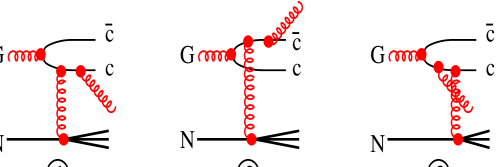
Figure 8: Born graphs contributing to $\bar{c}c$ pair production accompanied with radiation of a gluon.

The amplitude of $\bar{c}cG$ production corresponding to graphs 1-15 has the following structure,

$$A^{\bar{\mu}\mu}_{ij,ab}=\sum\limits_{l=1}^{15}\Bigl{(}A^{\bar{\mu}\mu}_{ij,ab}\Bigr{)}_{l}\ ,$$ (A.2)

where

$$\Bigl{(}A^{\bar{\mu}\mu}_{ij,ab}\Bigr{)}_{l}=\frac{i\,\sqrt{3}\,\alpha_{s}^{3/2}}{(k_{T}^{2}+\lambda^{2})\,D_{l}}\ \sum\limits_{d=1}^{N_{c}^{2}-1}T_{abd}^{(l)}(ij)\,F^{(d)}_{GN\to X}(k_{T},\{X\})\ \xi^{\mu}_{c}\Bigr{.}^{\dagger}\,\hat{\Gamma}_{l}\,\bar{\xi}^{\bar{\mu}}_{\bar{c}}\ .$$ (A.3)

Here $\lambda$ is the effective gluon mass aimed to incorporate confinement, its value we discuss later. The amplitude of gluon-absorption by a nucleon, $F^{(d)}_{GN\to X}(k_{T},\{X\})$, determines the unintegrated gluon density as it is introduced in (14),

$$\int d\{X\}\sum\limits_{d=1}^{8}\Bigl{|}F^{(d)}_{GN\to X}(k_{T},\{X\})\Bigr{|}^{2}=4\pi\,{\cal F}(k_{T}^{2},x)\ .$$ (A.4)

Here

$$x = \frac{M^{2}(\bar{c},c,G)}{s}\ ;$$ (A.5)

$$M^{2}_{\bar{c}cG} = \frac{m_{c}^{2}+k_{1}^{2}}{\alpha_{1}}+\frac{m_{c}^{2}+k_{2}^{2}}{\alpha_{2}}+\frac{\lambda^{2}+k_{3}^{2}}{\alpha_{3}}\ ,$$ (A.6)

where $\vec{k}_{1},\ \vec{k}_{2},\ \vec{k}_{3}$ and $\alpha_{1},\ \alpha_{2},\ \alpha_{3}$ are the transverse momenta and fractions of the initial light-cone momentum of the projectile gluon carried by the produced $\bar{c},\ c$ and $G$ (see Fig. 2), respectively, and

$$\vec{k}_{T}=\vec{k}_{1}+\vec{k}_{2}+\vec{k}_{3}\ .$$ (A.7)

The $3\times 3$ matrixes $T_{abd}^{(l)}(ij)$ in (A.3) act in the color space of the $\bar{c}c$ quarks, and the indexes $i,\ j$ corresponds to the $c$ and $\bar{c}$ respectively.

$$T^{(1)}_{abd} = \tau_{a}\,\tau_{d}\,\tau_{b}$$

$$T^{(2)}_{abd} = \tau_{b}\,\tau_{d}\,\tau_{a}$$

$$T^{(3)}_{abd} = \tau_{a}\,\tau_{b}\,\tau_{d}$$

$$T^{(4)}_{abd} = \tau_{d}\,\tau_{b}\,\tau_{a}$$

$$T^{(5)}_{abd} = \tau_{d}\,\tau_{a}\,\tau_{b}$$

$$T^{(6)}_{abd} = \tau_{b}\,\tau_{a}\,\tau_{d}$$

$$T^{(7)}_{abd} = i\,\sum\limits_{e=1}^{N_{c}^{2}-1}f_{ebd}\,\tau_{a}\,\tau_{e}\ ;$$

$$T^{(8)}_{abd} = i\,\sum\limits_{e=1}^{N_{c}^{2}-1}f_{edb}\,\tau_{e}\,\tau_{a}\ ;$$

$$T^{(9)}_{abd} = i\,\sum\limits_{e=1}^{N_{c}^{2}-1}f_{ade}\,\tau_{e}\,\tau_{b}\ ;$$

$$T^{(10)}_{abd} = i\,\sum\limits_{e=1}^{N_{c}^{2}-1}f_{ade}\,\tau_{b}\,\tau_{e}\ ;$$

$$T^{(11)}_{abd} = i\,\sum\limits_{e=1}^{N_{c}^{2}-1}f_{abe}\,\tau_{e}\,\tau_{d}\ ;$$

$$T^{(12)}_{abd} = i\,\sum\limits_{e=1}^{N_{c}^{2}-1}f_{abe}\,\tau_{d}\,\tau_{e}\ ;$$

$$T^{(13)}_{abd} = i\,\sum\limits_{e,g=1}^{N_{c}^{2}-1}f_{abe}\,f_{edg}\,\tau_{g}\ ;$$

$$T^{(14)}_{abd} = i\,\sum\limits_{e,g=1}^{N_{c}^{2}-1}f_{ade}\,f_{ebg}\,\tau_{g}\ ;$$

$$T^{(15)}_{abd} = i\,\sum\limits_{e,g=1}^{N_{c}^{2}-1}f_{ebd}\,f_{aeg}\,\tau_{g}\ .$$ (A.8)

Here $\lambda_{a}=\tau_{a}/2$ are the Gell-Mann matrixes.

Note that the matrixes $T^{(l)}_{abd}$ are not independent, but connected by linear relations (we skip the indexes $abd$),

$$T^{(3)}-T^{(1)}+T^{(7)} = 0\ ;$$

$$T^{(5)}-T^{(1)}+T^{(9)} = 0\ ;$$

$$T^{(4)}-T^{(2)}+T^{(8)} = 0\ ;$$

$$T^{(6)}-T^{(2)}+T^{(10)} = 0\ ;$$

$$T^{(13)}-T^{(11)}+T^{(13)} = 0\ ;$$

$$T^{(13)}+T^{(14)}+T^{(15)} = 0\ ;$$

$$T^{(15)}-T^{(7)}+T^{(8)} = 0\ ;$$

$$T^{(14)}-T^{(10)}+T^{(9)} = 0\ ;$$

The $c$-quark spinors $\xi$ in (A.3) are defined in (11); $\{X\}$ is the set of variables describing the state $X$; the 15 vertex functions $\hat{\Gamma}_{l}$ read,

$$\hat{\Gamma}_{1} = \hat{U}_{1}(\vec{k}_{1},\alpha_{1})\,\hat{V}_{1}(\vec{k}_{23},\alpha_{2},\alpha_{3})\ ;$$

$$\hat{\Gamma}_{2} = \hat{V}_{2}(\vec{k}_{13},\alpha_{1},\alpha_{3})\,\hat{U}_{2}(\vec{k}_{2},\alpha_{2})\,\ ;$$

$$\hat{\Gamma}_{3} = -\alpha_{1}\,\hat{U}_{1}(\vec{k}_{1},\alpha_{1})\,\hat{V}_{1}(\vec{k}_{23}-\alpha_{3}\vec{k}_{T},\alpha_{2},\alpha_{3})\ ;$$

$$\hat{\Gamma}_{4} = -\alpha_{2}\,\hat{V}_{2}(\vec{k}_{13}-\alpha_{3}\vec{k}_{T},\alpha_{1},\alpha_{3})\,\hat{U}_{2}(\vec{k}_{2},\alpha_{2})\,\ ;$$

$$\hat{\Gamma}_{5} = -\alpha_{2}\alpha_{3}\,\hat{U}_{1}(\vec{k}_{1}-\vec{k}_{T},\alpha_{1})\,\hat{V}_{1}(\vec{k}_{23},\alpha_{2},\alpha_{3})\ ;$$

$$\hat{\Gamma}_{6} = -\alpha_{1}\alpha_{3}\,\hat{V}_{2}(\vec{k}_{13},\alpha_{1},\alpha_{3})\,\hat{U}_{2}(\vec{k}_{2}-\vec{k}_{T},\alpha_{2})\,\ ;$$

$$\hat{\Gamma}_{7} = -\alpha_{1}\,\hat{U}_{1}(\vec{k}_{1},\alpha_{1})\,\hat{V}_{1}(\vec{k}_{23}+\alpha_{2}\vec{k}_{T},\alpha_{2},\alpha_{3})\ ;$$

$$\hat{\Gamma}_{8} = -\alpha_{2}\,\hat{V}_{2}(\vec{k}_{13}+\alpha_{1}\vec{k}_{T},\alpha_{1},\alpha_{3})\,\hat{U}_{2}(\vec{k}_{2},\alpha_{2})\,\ ;$$

$$\hat{\Gamma}_{9} = -\alpha_{2}\alpha_{3}\,\hat{U}_{1}(\vec{k}_{1}-\alpha_{1}\vec{k}_{T},\alpha_{1})\,\hat{V}_{1}(\vec{k}_{23},\alpha_{2},\alpha_{3})\ ;$$

$$\hat{\Gamma}_{10} = -\alpha_{1}\alpha_{3}\,\hat{V}_{2}(\vec{k}_{13},\alpha_{1},\alpha_{3})\,\hat{U}_{2}(\vec{k}_{2}-\alpha_{2}\vec{k}_{T},\alpha_{2})\ ;$$

$$\hat{\Gamma}_{11} = \alpha_{3}\,\hat{U}_{0}(\vec{k}_{12}+\alpha_{1}\vec{k}_{T},\alpha_{1},\alpha_{2})\,\hat{V}_{0}(\vec{k}_{3})\ ;$$

$$\hat{\Gamma}_{12} = -\alpha_{3}\,\hat{U}_{0}(\vec{k}_{12}-\alpha_{2}\vec{k}_{T},\alpha_{1},\alpha_{2})\,\hat{V}_{0}(\vec{k}_{3})\ ;$$

$$\hat{\Gamma}_{13} = \bar{\alpha}_{3}\,\hat{U}_{0}(\vec{k}_{12},\alpha_{1},\alpha_{2})\,\hat{V}_{0}(\vec{k}_{3})\ ;$$

$$\hat{\Gamma}_{14} = \alpha_{1}\alpha_{2}\,\hat{U}_{0}(\vec{k}_{12},\alpha_{1},\alpha_{2})\,\hat{V}_{0}(\vec{k}_{3})\ ;$$

$$\hat{\Gamma}_{15} = \alpha_{1}\alpha_{2}\,\hat{U}_{0}(\vec{k}_{12},\alpha_{1},\alpha_{2})\,\hat{V}_{0}(\vec{k}_{3}-\vec{k}_{T})\ .$$ (A.10)

Here

$$\vec{k}_{13}=\alpha_{3}\vec{k}_{1}-\alpha_{1}\vec{k}_{3}\ ;$$

$$\vec{k}_{23}=\alpha_{3}\vec{k}_{2}-\alpha_{2}\vec{k}_{3}\ ;$$

$$\alpha_{1}+\alpha_{2}+\alpha_{3}=1\ .$$ (A.11)

The matrixes $\hat{U}_{0,1,2}$ and $\hat{V}_{0,1,2}$ are defined as follows,

$$\hat{U}_{0}(\vec{k}_{12},\alpha_{1},\alpha_{2}) = (\alpha_{1}+\alpha_{2})m_{c}\,\vec{\sigma}\cdot\vec{e}+(\alpha_{2}-\alpha_{1})\,(\vec{\sigma}\cdot\vec{n})(\vec{e}_{in}\cdot\vec{k}_{12})+i\,(\vec{e}_{in}\times\vec{n})\cdot\vec{k}_{12}\ ;$$

$$\hat{U}_{1}(\vec{k}_{1},\alpha_{1}) = m_{c}\,\vec{\sigma}\cdot\vec{e}+(1-2\alpha_{1})\,(\vec{\sigma}\cdot\vec{n})(\vec{e}_{in}\cdot\vec{k}_{1})+i\,(\vec{e}_{in}\times\vec{n})\cdot\vec{k}_{1}\ ;$$

$$\hat{U}_{2}(\vec{k}_{2},\alpha_{2}) = m_{c}\,\vec{\sigma}\cdot\vec{e}+(1-2\alpha_{2})\,(\vec{\sigma}\cdot\vec{n})(\vec{e}_{in}\cdot\vec{k}_{2})-i\,(\vec{e}_{in}\times\vec{n})\cdot\vec{k}_{2}\ ;$$ (A.12)

$$\hat{V}_{0}(\vec{k}_{3}) = \vec{e}_{f}\cdot\vec{k}_{3}\ ;$$

$$\hat{V}_{1}(\vec{k}_{23},\alpha_{2},\alpha_{3}) = (2\alpha_{2}+\alpha_{3})\,\vec{k}_{23}\cdot\vec{e}_{f}+i\,m_{c}\,\alpha_{3}^{2}\,(\vec{n}\times\vec{e}_{f})\cdot\vec{\sigma}-i\,\alpha_{3}\,(\vec{k}_{23}\times\vec{e}_{f})\cdot\vec{\sigma}\ ;$$

$$\hat{V}_{2}(\vec{k}_{13},\alpha_{1},\alpha_{3}) = (2\alpha_{1}+\alpha_{3})\,\vec{k}_{13}\cdot\vec{e}_{f}-i\,m_{c}\,\alpha_{3}^{2}\,(\vec{n}\times\vec{e}_{f})\cdot\vec{\sigma}+i\,\alpha_{3}\,(\vec{k}_{13}\times\vec{e}_{f})\cdot\vec{\sigma}\ ,$$

where $\vec{e}_{in}$ and $\vec{e}_{f}$ are the polarization vectors of the initial and radiated gluons respectively.

The functions $D_{l}$ in the denominator of (A.3) read,

$$D_{1} = \Delta_{0}(\vec{k}_{1},\alpha_{1})\,\Delta_{2}(\vec{k}_{23},\alpha_{2},\alpha_{3})\ ;$$

$$D_{2} = \Delta_{0}(\vec{k}_{2},\alpha_{2})\,\Delta_{2}(\vec{k}_{13},\alpha_{1},\alpha_{3})\ ;$$

$$D_{3} = \Delta_{0}(\vec{k}_{1},\alpha_{1})\,\Delta_{1}(\vec{k}_{1},\vec{k}_{23}-\alpha_{3}\vec{k}_{T},\alpha_{1},\alpha_{2},\alpha_{3})\ ;$$

$$D_{4} = \Delta_{0}(\vec{k}_{2},\alpha_{2})\,\Delta_{1}(\vec{k}_{2},\vec{k}_{13}-\alpha_{3}\vec{k}_{T},\alpha_{2},\alpha_{1},\alpha_{3})\ ;$$

$$D_{5} = \Delta_{1}(\vec{k}_{1}-\vec{k}_{T},\vec{k}_{23},\alpha_{1},\alpha_{2},\alpha_{3})\,\Delta_{2}(\vec{k}_{23},\alpha_{2},\alpha_{3})\ ;$$

$$D_{6} = \Delta_{1}(\vec{k}_{2}-\vec{k}_{T},\vec{k}_{13},\alpha_{2},\alpha_{1},\alpha_{3})\,\Delta_{2}(\vec{k}_{13},\alpha_{1},\alpha_{3})\ ;$$

$$D_{7} = \Delta_{0}(\vec{k}_{1},\alpha_{1})\,\Delta_{1}(\vec{k}_{1},\vec{k}_{23}+\alpha_{2}\vec{k}_{T},\alpha_{1},\alpha_{2},\alpha_{3})\ ;$$

$$D_{8} = \Delta_{0}(\vec{k}_{2},\alpha_{2})\,\Delta_{1}(\vec{k}_{2},\vec{k}_{13}+\alpha_{1}\vec{k}_{T},\alpha_{2},\alpha_{1},\alpha_{3})\ ;$$

$$D_{9} = \Delta_{2}(\vec{k}_{23},\alpha_{2},\alpha_{3})\,\Delta_{1}(\vec{k}_{1}-\alpha_{1}\vec{k}_{T},\vec{k}_{23},\alpha_{1},\alpha_{2},\alpha_{3})\ ;$$

$$D_{10} = \Delta_{2}(\vec{k}_{13},\alpha_{1},\alpha_{3})\,\Delta_{1}(\vec{k}_{2}-\alpha_{2}\vec{k}_{T},\vec{k}_{13},\alpha_{2},\alpha_{1},\alpha_{3})\ ;$$

$$D_{11} = \Delta_{3}(\vec{k}_{3},\alpha_{1},\alpha_{3})\,\Delta_{4}(\vec{k}_{3},\vec{k}_{12}+\alpha_{1}\vec{k}_{T},\alpha_{1},\alpha_{2},\alpha_{3})\ ;$$

$$D_{12} = \Delta_{3}(\vec{k}_{3},\alpha_{1},\alpha_{3})\,\Delta_{4}(\vec{k}_{3},\vec{k}_{12}-\alpha_{2}\vec{k}_{T},\alpha_{1},\alpha_{2},\alpha_{3})\ ;$$

$$D_{13} = \Delta_{3}(\vec{k}_{3},\alpha_{1},\alpha_{3})\,\Delta_{5}(\vec{k}_{12},\alpha_{1},\alpha_{2},\alpha_{3})\ ;$$

$$D_{14} = \Delta_{5}(\vec{k}_{12},\alpha_{1},\alpha_{2},\alpha_{3})\,\Delta_{4}(\vec{k}_{31}+\vec{k}_{32},\vec{k}_{12},\alpha_{1},\alpha_{2},\alpha_{3})\ ;$$

$$D_{15} = \Delta_{5}(\vec{k}_{12},\alpha_{1},\alpha_{2},\alpha_{3})\,\Delta_{4}(\vec{k}_{3}-\vec{k}_{T},\vec{k}_{12},\alpha_{1},\alpha_{2},\alpha_{3})\ ,$$ (A.14)

where

$$\Delta_{0}(\vec{k}_{1},\alpha_{1}) = m_{c}^{2}+k_{1}^{2}-\alpha_{1}\bar{\alpha}_{1}\,\lambda^{2}\ ;$$

$$\Delta_{1}(\vec{k}_{1},\vec{k}_{23},\alpha_{1},\alpha_{2},\alpha_{3}) = \bar{\alpha}_{1}\bar{\alpha}_{3}(\alpha_{3}\,m_{c}^{2}+\alpha_{1}\alpha_{2}\,\lambda^{2})+\alpha_{1}k_{23}^{2}+\alpha_{2}\alpha_{2}\,k_{1}^{2}\ ;$$

$$\Delta_{2}(\vec{k}_{13},\alpha_{1},\alpha_{3}) = \alpha_{3}^{2}\,m_{c}^{2}+\alpha_{1}(\alpha_{1}+\alpha_{3})\,\lambda^{2}+k_{13}^{2}\ ;$$

$$\Delta_{3}(\vec{k}_{3},\alpha_{1},\alpha_{3}) = k_{3}^{2}+[1-\alpha_{3}(\alpha_{1}+\alpha_{1})]\,\lambda^{2}\ ;$$

$$\Delta_{4}(\vec{k}_{3},\vec{k}_{12},\alpha_{1},\alpha_{2},\alpha_{3}) = \bar{\alpha}_{3}(\alpha_{3}\,m_{c}^{2}+\alpha_{1}\alpha_{2}\,\lambda^{2})+\frac{\alpha_{1}\alpha_{2}}{\bar{\alpha}_{3}}\,k_{3}^{2}+\frac{\alpha_{3}}{\bar{\alpha}_{3}}\,k_{12}^{2}\ ;$$

$$\Delta_{5}(\vec{k}_{12},\alpha_{1},\alpha_{2},\alpha_{3}) = \bar{\alpha}_{3}^{2}\,m_{c}^{2}-\alpha_{1}\alpha_{2}\,\lambda^{2}+k_{12}^{2}\ .$$ (A.15)

Functions $\Delta_{0}$ - $\Delta_{5}$ are not independent, but satisfy the relation

$$\Bigl{[}\Delta_{0}(\vec{k}_{1},\alpha_{1})\,\Delta_{2}(\vec{k}_{23},\alpha_{2},\alpha_{3})\Bigr{]}^{-1}=\alpha_{1}\,\Bigl{[}\Delta_{0}(\vec{k}_{1},\alpha_{1})\,\Delta_{1}(\vec{k}_{1},\vec{k}_{23},\alpha_{1},\alpha_{2},\alpha_{3})\Bigr{]}^{-1}$$

$$+ \alpha_{2}\alpha_{3}\,\Bigl{[}\Delta_{2}(\vec{k}_{23},\alpha_{2},\alpha_{3})\,\Delta_{1}(\vec{k}_{1},\vec{k}_{23},\alpha_{1},\alpha_{2},\alpha_{3})\Bigr{]}^{-1}\ ;$$

$$\Bigl{[}\Delta_{3}(\vec{k}_{3},\alpha_{1},\alpha_{3})\,\Delta_{5}(\vec{k}_{12},\alpha_{1},\alpha_{2},\alpha_{3})\Bigr{]}^{-1}=\frac{\alpha_{1}\alpha_{2}}{\bar{\alpha}_{3}}$$

$$\times \Bigl{[}\Delta_{4}(\vec{k}_{3},\vec{k}_{12},\alpha_{1},\alpha_{2},\alpha_{3})\,\Delta_{5}(\vec{k}_{12},\alpha_{1},\alpha_{2},\alpha_{3})\Bigr{]}^{-1}$$

$$+ \frac{\alpha_{3}}{\bar{\alpha}_{3}}\,\Bigl{[}\Delta_{4}(\vec{k}_{3},\vec{k}_{12},\alpha_{1},\alpha_{2},\alpha_{3})\,\Delta_{3}(\vec{k}_{3},\alpha_{1},\alpha_{3})\Bigr{]}^{-1}\ .$$ (A.17)

The sum of the 15 amplitudes Eq. (A.3) is convenient to split up into 9 terms,

$$\hat{M}=\sum\limits_{l=1}^{15}T^{(l)}\,\frac{\hat{\Gamma}_{l}}{D_{l}}=\sum\limits_{i=1}^{9}S^{(i)}\,\hat{M}_{i}\ ,$$ (A.18)

where matrixes $S^{(i)}$ are related to $T^{(l)}$ in (A.8) as,

$$S^{(1)} = T^{(1)}\ ;\ \ \ \ \ \ \ S^{(2)}=T^{(2)}\ ;$$

$$S^{(3)} = T^{(7)}\ ;\ \ \ \ \ \ \ S^{(4)}=T^{(8)}\ ;$$

$$S^{(5)} = T^{(9)}\ ;\ \ \ \ \ \ \ S^{(6)}=T^{(10)}\ ;$$

$$S^{(7)} = {1\over 2}\,\Bigl{(}T^{(11)}+T^{(12)}\Bigr{)}\ ;$$

$$S^{(8)} = T^{(14)}\ ;\ \ \ \ \ \ \ S^{(9)}=T^{(15)}\ .$$ (A.19)

The matrixes $\hat{M}_{i}$ can be represented in the following form using relations (Appendix A), (A.19),

$$\hat{M}_{1} = \alpha_{1}\,\hat{\nu}_{1}(\vec{k}_{1},\alpha_{1})\,\Bigl{[}\hat{\mu}_{1}(\vec{k}_{1},\vec{k}_{23},\alpha_{1},\alpha_{2},\alpha_{3})-\hat{\mu}_{1}(\vec{k}_{1},\vec{k}_{23}-\alpha_{3}\vec{k}_{T},\alpha_{1},\alpha_{2},\alpha_{3})\Bigr{]}$$ (A.20)

$$+ \alpha_{2}\alpha_{3}\,\Bigl{[}\hat{\lambda}_{1}(\vec{k}_{1},\vec{k}_{23},\alpha_{1},\alpha_{2},\alpha_{3})$$

$$- \hat{\lambda}_{1}(\vec{k}_{1}-\vec{k}_{T},\vec{k}_{23},\alpha_{1},\alpha_{2},\alpha_{3})\Bigr{]}\,\hat{\rho}_{1}(\vec{k}_{23},\alpha_{2},\alpha_{3})\ ;$$

$$\hat{M}_{2} = \alpha_{2}\,\Bigl{[}\hat{\mu}_{2}(\vec{k}_{2},\vec{k}_{13},\alpha_{2},\alpha_{1},\alpha_{3})-\hat{\mu}_{2}(\vec{k}_{2},\vec{k}_{13}-\alpha_{3}\vec{k}_{T},\alpha_{1},\alpha_{2},\alpha_{3})\Bigr{]}\,\hat{\nu}_{2}(\vec{k}_{2},\alpha_{2})$$ (A.21)

$$+ \alpha_{1}\alpha_{3}\,\hat{\rho}_{2}(\vec{k}_{13},\alpha_{1},\alpha_{3})\,\Bigl{[}\hat{\lambda}_{2}(\vec{k}_{2},\vec{k}_{13},\alpha_{2},\alpha_{1},\alpha_{3})$$

$$- \hat{\lambda}_{2}(\vec{k}_{2}-\vec{k}_{T},\vec{k}_{13},\alpha_{1},\alpha_{2},\alpha_{3})\Bigr{]}$$

$$\hat{M}_{3} = \alpha_{1}\,\hat{\nu}_{1}(\vec{k}_{1},\alpha_{1})\,\Bigl{[}\hat{\mu}_{1}(\vec{k}_{1},\vec{k}_{23}-\alpha_{3}\vec{k}_{T},\alpha_{1},\alpha_{2},\alpha_{3})$$ (A.22)

$$- \hat{\mu}_{1}(\vec{k}_{1},\vec{k}_{23}+\alpha_{2}\vec{k}_{T},\alpha_{1},\alpha_{2},\alpha_{3})\Bigr{]}\ ;$$

$$\hat{M}_{4} = \alpha_{2}\,\Bigl{[}\hat{\mu}_{2}(\vec{k}_{2},\vec{k}_{13}-\alpha_{3}\vec{k}_{T},\alpha_{2},\alpha_{1},\alpha_{3})$$ (A.23)

$$- \hat{\mu}_{2}(\vec{k}_{2},\vec{k}_{13}+\alpha_{1}\vec{k}_{T},\alpha_{1},\alpha_{2},\alpha_{3})\Bigr{]}\,\hat{\nu}_{2}(\vec{k}_{2},\alpha_{2})\ ;$$

$$\hat{M}_{5} = \alpha_{2}\alpha_{3}\,\Bigl{[}\hat{\lambda}_{1}(\vec{k}_{1}-\vec{k}_{T},\vec{k}_{23},\alpha_{1},\alpha_{2},\alpha_{3})$$ (A.24)

$$- \hat{\lambda}_{1}(\vec{k}_{1}-\alpha_{1}\vec{k}_{T},\vec{k}_{23},\alpha_{1},\alpha_{2},\alpha_{3})\Bigr{]}\,\hat{\rho}_{1}(\vec{k}_{23},\alpha_{2},\alpha_{3})\ ;$$

$$\hat{M}_{6} = \alpha_{1}\alpha_{3}\,\hat{\rho}_{2}(\vec{k}_{13},\alpha_{1},\alpha_{3})\,\Bigl{[}\hat{\lambda}_{2}(\vec{k}_{2}-\vec{k}_{T},\vec{k}_{13},\alpha_{1},\alpha_{2},\alpha_{3})$$ (A.25)

$$- \hat{\lambda}_{2}(\vec{k}_{2}-\alpha_{2}\vec{k}_{T},\vec{k}_{13},\alpha_{1},\alpha_{2},\alpha_{3})\Bigr{]}\ ;$$

$$\hat{M}_{7} = \alpha_{3}\,\hat{\phi}(\vec{k}_{3},\alpha_{1},\alpha_{2},\alpha_{3})\,\Bigl{[}\hat{\omega}(\vec{k}_{3},\vec{k}_{12}+\alpha_{1}\vec{k}_{T},\alpha_{1},\alpha_{2},\alpha_{3})$$ (A.26)

$$- \hat{\omega}(\vec{k}_{3},\vec{k}_{12}-\alpha_{2}\vec{k}_{T},\alpha_{1},\alpha_{2},\alpha_{3})\Bigr{]}\ ;$$

$$\hat{M}_{8} = {1\over 2}\,\alpha_{3}\,\hat{\phi}(\vec{k}_{3},\alpha_{1},\alpha_{2},\alpha_{3})\,\Bigl{[}\hat{\omega}(\vec{k}_{3},\vec{k}_{12}+\alpha_{1}\vec{k}_{T},\alpha_{1},\alpha_{2},\alpha_{3})$$ (A.27)

$$+ \hat{\omega}(\vec{k}_{3},\vec{k}_{12}-\alpha_{2}\vec{k}_{T},\alpha_{1},\alpha_{2},\alpha_{3})-2\,\hat{\omega}(\vec{k}_{3},\vec{k}_{12},\alpha_{1},\alpha_{2},\alpha_{3})\Bigr{]}\ ;$$

$$\hat{M}_{9} = \Bigl{[}\hat{\beta}(\vec{k}_{3},\vec{k}_{12},\alpha_{1},\alpha_{2},\alpha_{3})-\hat{\beta}(\vec{k}_{3}-\vec{k}_{T},\vec{k}_{12},\alpha_{1},\alpha_{2},\alpha_{3})\Bigr{]}$$ (A.28)

$$\times \hat{\gamma}(\vec{k}_{12},\alpha_{1},\alpha_{2},\alpha_{3})\ .$$

The following notations are used here,

$$\hat{\nu}_{1}(\vec{k}_{1},\alpha_{1}) = \frac{\hat{U}_{1}(\vec{k}_{1},\alpha_{1})}{\Delta_{0}(\vec{k}_{1},\alpha_{1})}\ ;$$

$$\hat{\nu}_{2}(\vec{k}_{2},\alpha_{2}) = \frac{\hat{U}_{2}(\vec{k}_{2},\alpha_{2})}{\Delta_{0}(\vec{k}_{2},\alpha_{2})}\ ;$$ (A.29)

$$\hat{\mu}_{1}(\vec{k}_{1},\vec{k}_{23},\alpha_{1},\alpha_{2},\alpha_{3}) = \frac{\hat{V}_{1}(\vec{k}_{23},\alpha_{2},\alpha_{3})}{\Delta_{1}(\vec{k}_{1},\vec{k}_{23},\alpha_{1},\alpha_{2},\alpha_{3})}\ ;$$

$$\hat{\mu}_{2}(\vec{k}_{2},\vec{k}_{13},\alpha_{1},\alpha_{2},\alpha_{3}) = \frac{\hat{V}_{2}(\vec{k}_{13},\alpha_{1},\alpha_{3})}{\Delta_{1}(\vec{k}_{2},\vec{k}_{13},\alpha_{1},\alpha_{2},\alpha_{3})}\ ;$$ (A.30)

$$\hat{\lambda}_{1}(\vec{k}_{1},\vec{k}_{23},\alpha_{1},\alpha_{2},\alpha_{3}) = \frac{\hat{U}_{1}(\vec{k}_{1},\alpha_{1})}{\Delta_{1}(\vec{k}_{1},\vec{k}_{23},\alpha_{1},\alpha_{2},\alpha_{3})}\ ;$$

$$\hat{\lambda}_{2}(\vec{k}_{2},\vec{k}_{13},\alpha_{1},\alpha_{2},\alpha_{3}) = \frac{\hat{U}_{2}(\vec{k}_{2},\alpha_{2})}{\Delta_{1}(\vec{k}_{2},\vec{k}_{13},\alpha_{1},\alpha_{2},\alpha_{3})}\ ;$$ (A.31)

$$\hat{\rho}_{1}(\vec{k}_{23},\alpha_{2},\alpha_{3}) = \frac{\hat{V}_{1}(\vec{k}_{23},\alpha_{2},\alpha_{3})}{\Delta_{2}(\vec{k}_{23},\alpha_{2},\alpha_{3})}\ ;$$

$$\hat{\rho}_{2}(\vec{k}_{13},\alpha_{1},\alpha_{3}) = \frac{\hat{V}_{2}(\vec{k}_{13},\alpha_{1},\alpha_{3})}{\Delta_{2}(\vec{k}_{13},\alpha_{1},\alpha_{3})}\ ;$$ (A.32)

$$\hat{\beta}(\vec{k}_{3},\vec{k}_{12},\alpha_{1},\alpha_{2},\alpha_{3})=\frac{\hat{V}_{0}(k_{3})}{\Delta_{4}(\vec{k}_{3},\vec{k}_{12},\alpha_{1},\alpha_{2},\alpha_{3})}\ ;$$ (A.33)

$$\hat{\gamma}(\vec{k}_{12},\alpha_{1},\alpha_{2},\alpha_{3})=\frac{\hat{U}_{0}(k_{12},\alpha_{1},\alpha_{2})}{\Delta_{5}(\vec{k}_{12},\alpha_{1},\alpha_{2},\alpha_{3})}\ ;$$ (A.34)

$$\hat{\omega}(\vec{k}_{3},\vec{k}_{12},\alpha_{1},\alpha_{2},\alpha_{3})=\frac{\hat{U}_{0}(k_{12},\alpha_{1},\alpha_{2})}{\Delta_{4}(\vec{k}_{3},\vec{k}_{12},\alpha_{1},\alpha_{2},\alpha_{3})}\ ;$$ (A.35)

$$\hat{\phi}(\vec{k}_{3},\vec{k}_{12},\alpha_{1},\alpha_{2})=\frac{\hat{V}_{0}(k_{3})}{\Delta_{3}(\vec{k}_{3},\alpha_{1},\alpha_{3})}\ ;$$ (A.36)

Apparently, the amplitude operators in Eqs. (A.20)-(A.28) vanish, in forward direction, $\vec{k}_{T}\to 0$, what guarantees infra-red stability of the cross section of gluon radiation.

The above relations are valid at any values of $\alpha_{1},\ \alpha_{2},\ \alpha_{3}$, however they substantially simplify if the momentum fraction carried by the radiated gluon is small, $\alpha_{3}\ll 1$ what corresponds to th dominant configuration for a fluctuation $G\to\bar{c}cG$. In the limit $\alpha_{3}\to 0$ the amplitudes $M_{1},\ M_{2},\ M_{5},\ M_{6},\ M_{7}$ and $M_{8}$ vanish. Also the operators $\hat{V}_{1,2}$ do not depend any more on the spin matrix $\vec{\sigma}$ and become proportional $\hat{V}_{0}$

$$\hat{V}_{1}(\vec{k}_{23},\alpha_{2},\alpha_{3})\Bigr{|}_{\alpha_{3}\to 0} = -\alpha_{2}^{2}\,\hat{V}_{0}(\vec{k})\ ;$$

$$\hat{V}_{2}(\vec{k}_{13},\alpha_{1},\alpha_{3})\Bigr{|}_{\alpha_{3}\to 0} = -\alpha_{1}^{2}\,\hat{V}_{0}(\vec{k})\ ;$$

$$\hat{V}_{1}(\vec{k}_{23}+\vec{\alpha}_{2}\vec{k}_{T},\alpha_{2},\alpha_{3})\Bigr{|}_{\alpha_{3}\to 0} = -\alpha_{2}^{2}\,\hat{V}_{0}(\vec{k}-\vec{k}_{T})\ ;$$

$$\hat{V}_{2}(\vec{k}_{13}+\alpha_{1}\vec{k}_{T},\alpha_{1},\alpha_{3})\Bigr{|}_{\alpha_{3}\to 0} = -\alpha_{1}^{2}\,\hat{V}_{0}(\vec{k}-\vec{k}_{T})\ .$$ (A.37)

Also the matrixes $\hat{U}_{1,2}\propto\hat{U}_{0}$,

$$\hat{U}_{1}(\vec{k}_{1},\alpha_{1})\Bigr{|}_{\alpha_{3}\to 0} = \hat{U}_{0}(\vec{k}_{12}+\alpha_{1}\vec{k}_{T},\alpha_{1},\alpha_{2})\ ;$$

$$\hat{U}_{2}(\vec{k}_{2},\alpha_{2})\Bigr{|}_{\alpha_{3}\to 0} = \hat{U}_{0}(\vec{k}_{12}-\alpha_{2}\vec{k}_{T},\alpha_{1},\alpha_{2})\ .$$ (A.38)

Besides, $\alpha_{1}+\alpha_{2}=\bar{\alpha}_{3}\approx 1$ and the denominators $\Delta_{i}$ take the simple form,

$$\Delta_{0}(\vec{k}_{1},\alpha_{1})\Bigr{|}_{\alpha_{3}\to 0} = m_{c}^{2}+k_{1}^{2}-\alpha_{1}\alpha_{2}\,\lambda^{2}\ ;$$

$$\Delta_{0}(\vec{k}_{2},\alpha_{1})\Bigr{|}_{\alpha_{3}\to 0} = m_{c}^{2}+k_{2}^{2}-\alpha_{1}\alpha_{2}\,\lambda^{2}\ ;$$

$$\Delta_{5}(\vec{k}_{12},\alpha_{1},\alpha_{2},\alpha_{3})\Bigr{|}_{\alpha_{3}\to 0} = m_{c}^{2}+k_{12}^{2}-\alpha_{1}\alpha_{2}\,\lambda^{2}\ ;$$

$$\Delta_{1}(\vec{k}_{1},\vec{k}_{23},\alpha_{1},\alpha_{2},\alpha_{3})\Bigr{|}_{\alpha_{3}\to 0} = \alpha_{2}\alpha_{1}^{2}\,\Bigl{[}k_{3}^{2}+\tau^{2}(k_{1}^{2})\Bigr{]}\ ;$$

$$\Delta_{1}(\vec{k}_{2},\vec{k}_{13},\alpha_{1},\alpha_{2},\alpha_{3})\Bigr{|}_{\alpha_{3}\to 0} = \alpha_{1}\alpha_{2}^{2}\,\Bigl{[}k_{3}^{2}+\tau^{2}(k_{2}^{2})\Bigr{]}\ ;$$

$$\Delta_{4}(\vec{k}_{3},\vec{k}_{12},\alpha_{1},\alpha_{2},\alpha_{3})\Bigr{|}_{\alpha_{3}\to 0} = \alpha_{1}\alpha_{2}\,\Bigl{[}k_{3}^{2}+\tau^{2}(k_{12}^{2})\Bigr{]}\ ,$$ (A.39)

where

$$\tau^{2}(\vec{k})=\frac{\alpha_{3}}{\alpha_{1}\alpha_{2}}\,(m_{c}^{2}+k^{2})+\lambda^{2}\ .$$ (A.40)

We keep the term linear in $\alpha_{3}$ in (A.40) since it is responsible for suppression of gluon radiation with

$$\alpha_{3}\mathrel{\hbox to0.0pt{\lower 4.0pt\hbox{\hskip 1.0pt$\sim$}\hss}\raise 1.0pt\hbox{$>$}}\frac{\lambda^{2}}{M^{2}_{\bar{c}c}}\ ,$$ (A.41)

where

$$M^{2}_{\bar{c}c}=\frac{m_{c}^{2}+k_{2}^{2}}{\alpha\bar{\alpha}}$$ (A.42)

is the invariant mass squared of the $\bar{c}c$ pair, and

$$\vec{k}_{12}=\bar{\alpha}\vec{k}_{1}-\alpha\vec{k}_{2}\ .$$ (A.43)

The approximation $\alpha_{3}\ll 1$ is justified even for gluons satisfying the condition Eq. (A.41), since

$$\frac{\lambda^{2}}{M^{2}_{\bar{c}c}}\sim\frac{\Lambda_{QCD}^{2}}{4\,m_{c}^{2}}\sim 0.005\ .$$ (A.44)

Further, we will make use of the relations,

$$\vec{k}_{1} = \vec{k}_{12}+\alpha(\vec{k}_{T}-\vec{k}_{3})+O(\alpha_{3})$$

$$\vec{k}_{2} = \vec{k}_{12}+\bar{\alpha}(\vec{k}_{T}-\vec{k}_{3})+O(\alpha_{3})\ ,$$ (A.45)

where $\alpha=\alpha_{1}$, and also take into account that both $k_{T}$ and $k_{3}$ are of the order of $\lambda$, i.e. they are much smaller than the typical values of $k_{12}\sim m_{c}$. Therefore, we will rely on the relations,

$$\tau^{2}(k_{1})\approx\tau^{2}(k_{2})\approx\tau^{2}(k_{12})\approx\tau^{2}=\lambda^{2}+\alpha_{3}\,M_{\bar{c}c}^{2}\ .$$ (A.46)

Within this approximation the amplitude of reaction $GN\to\bar{c}c\,G\,X$ at $\alpha_{3}\ll 1$ is given by

$$A_{ij,ab}^{\bar{\mu}\mu}=i\alpha_{s}^{3/2}\sum\limits_{e,d=1}^{N_{c}^{2}-1}\frac{f_{bde}\,F^{d}_{GN\to X}(\vec{k}_{T},\{x\})}{k_{T}^{2}+\lambda^{2}}\ \xi^{\mu}_{c}\Bigr{.}^{\dagger}\left\{\frac{\hat{U}_{0}(\vec{k}_{1},\alpha,\bar{\alpha})}{k_{1}^{2}+m_{c}^{2}}\,(\tau_{e}\,\tau_{a})_{ij}\right.$$ (A.47)

$$- \left.\frac{\hat{U}_{0}(-\vec{k}_{2},\alpha,\bar{\alpha})}{k_{2}^{2}+m_{c}^{2}}\,(\tau_{a}\,\tau_{e})_{ij}+i\,\frac{\hat{U}_{0}(\vec{k}_{12},\alpha,\bar{\alpha})}{k_{12}^{2}+m_{c}^{2}}\,\sum\limits_{g=1}^{N_{c}^{2}-1}f_{aeg}\,(\tau_{g})_{ij}\right\}\tilde{\xi}_{\bar{c}}^{\bar{\mu}}$$

$$\times \left[\frac{2\vec{e}_{f}\cdot(\vec{k}_{3}-\vec{k}_{T})}{(\vec{k}_{3}-\vec{k}_{T})^{2}+\tau^{2}}-\frac{2\,\vec{e}_{f}\cdot\vec{k}_{3}}{\vec{k}_{3}^{2}+\tau^{2}}\right]\ .$$

To switch to the impact parameter representation we should perform Fourier integration over momenta $\vec{k}_{12},\ \vec{k}_{T}$ and $\vec{k}_{3}$. This procedure turns out to be quite complicated because of the dependence of $\tau$ in (A.46) on the invariant mass Eq. (A.42) which involves $\vec{k}_{12}$. For the sake of simplicity we replace in Eqs. (A.46) – (A.47) the invariant mass of the $\bar{c}c$ pair by its mean value, $M_{\bar{c}c}^{2}\Rightarrow\overline{M_{\bar{c}c}^{2}}=N\,4m_{c}^{2}$, where $N\sim 1-2$. Then Eq. (A.47) can be represented in the form,

$$A_{ij,ab}^{\bar{\mu}\mu}=3i\sum\limits_{e,d=1}^{N_{c}^{2}-1}f_{bde}\int d^{2}r\,d^{2}\rho\,d^{2}s\,\exp\Bigl{(}i\,\vec{k}_{12}\cdot\vec{r}+i\,\vec{k}_{3}\cdot\vec{\rho}+i\,\vec{k}_{T}\cdot\vec{s}\Bigr{)}$$ (A.48)

$$\times \Psi^{\bar{\mu}\mu}(\vec{r},\alpha)\,\Biggl{\{}\Phi_{cG}(\vec{\rho}+\alpha\vec{r})\ (\tau_{a}\tau_{e})_{ij}\,\Bigl{[}\gamma^{(d)}(\vec{\rho}+\vec{s})-\gamma^{(d)}(\vec{s}-\alpha\vec{r})\Bigr{]}$$

$$- \left.\Phi_{cG}\Bigl{(}\vec{\rho}-\bar{\alpha}\vec{r}\Bigr{)}\ (\tau_{e}\tau_{a})_{ij}\,\Bigl{[}\gamma^{(d)}(\vec{\rho}+\vec{s})-\gamma^{(d)}\Bigl{(}\vec{s}+\bar{\alpha}\vec{r}\Bigr{)}\Bigr{]}\right.$$

$$+ \Phi_{cG}(\vec{\rho})\,\sum\limits_{g=1}f_{eag}\ (\tau_{g})_{ij}\,\Bigl{[}\gamma^{(d)}(\vec{\rho}+\vec{s})-\gamma^{(d)}(\vec{s})\Bigr{]}\ ,\Biggr{\}}$$

where $\vec{r}$, $\vec{\rho}$ and $\vec{s}$ are the inter-quark separation, gluon – $\bar{c}c$ separation, and the position of the center of gravity of the whole $\bar{c}cG$ system, respectively. The $\bar{c}c$ LC wave function $\Psi^{\bar{\mu}\mu}(\vec{r},\alpha)$ and the profile function $\gamma^{(d)}(\vec{s})$ are defined in (11) and (13), respectively, and

$$\Phi_{cG}(\vec{\rho})=\frac{2i\sqrt{\alpha_{s}}}{\pi\sqrt{3}}\ \vec{e}_{f}\cdot\vec{\nabla}_{\rho}\ K_{0}(\tau\rho)\ .$$ (A.49)

Further, note that the mean $\bar{c}c$ separation $\sim 1/m_{c}$ is much smaller than the typical scale $\sim 1/\lambda\sim 1/\Lambda_{QCD}\sim 1\,\,\mbox{fm}$ of variation of the profile function $\gamma^{(d)}(s)$. Therefore, we can neglect the $\vec{r}$-dependence of $\gamma^{(d)}$ in (A.48), i.e. replace

$$\gamma^{(d)}(\vec{s}-\alpha r) \Rightarrow \gamma^{(d)}(\vec{s})\ ,$$

$$\gamma^{(d)}\Bigl{(}\vec{s}+\bar{\alpha}r\Bigr{)} \Rightarrow \gamma^{(d)}(\vec{s})\ .$$ (A.50)

After replacing the bilinear to linear combinations of $\tau$-matrixes in (A.48) by means of relation

$$(\tau_{a}\tau_{e})_{ij}={1\over 6}\,\delta_{ae}\,\delta_{ij}+{1\over 2}\sum\limits_{g=1}^{N_{c}^{2}-1}(d_{aeg}+if_{aeg})\,(\tau_{g})_{ij}\ ,$$ (A.51)

we arrive at the final result of this section,

$$A_{ij,ab}^{\bar{\mu}\mu}=3i\sum\limits_{e,d=1}^{N_{c}^{2}-1}f_{bde}\int d^{2}r\,d^{2}\rho\,d^{2}s\,\exp\Bigl{(}i\,\vec{k}_{12}\cdot\vec{r}+i\,\vec{k}_{3}\cdot\vec{\rho}+i\,\vec{k}_{T}\cdot\vec{s}\Bigr{)}\,\Bigl{[}\gamma^{(d)}(\vec{\rho}+\vec{s})-\gamma^{(d)}(\vec{s})\Bigr{]}$$ (A.52)

$$\times \Psi^{\bar{\mu}\mu}(\vec{r},\alpha)\,\Biggl{\{}\left[\,{1\over 6}\,\delta_{ae}\delta_{ij}+{1\over 2}\sum\limits_{g}d_{aeg}(\tau_{g})_{ij}\,\right]\,\Phi^{-}_{cG}(\vec{r},\vec{\rho})+{i\over 2}\sum\limits_{g}f_{aeg}(\tau_{g})_{ij}\,\Phi^{+}_{cG}(\vec{r},\vec{\rho})\Biggr{\}}\ .$$

Here

$$\Phi^{-}_{cG}(\vec{r},\vec{\rho}) = \Phi_{cG}(\vec{\rho}+\alpha\,\vec{r})-\Phi^{-}_{cG}\Bigl{(}\vec{\rho}-\bar{\alpha}\vec{r}\Bigr{)}\ ;$$

$$\Phi^{+}_{cG}(\vec{r},\vec{\rho}) = \Phi_{cG}(\vec{\rho}+\alpha\,\vec{r})+\Phi^{-}_{cG}\Bigl{(}\vec{\rho}-\bar{\alpha}\vec{r}\Bigr{)}-2\,\Phi_{cG}(\vec{\rho})\ .$$ (A.53)

The three terms in curly brackets in Eq. (A.52) describe production of the $\bar{c}c$ pair in different color and spin states. The first term containing $\delta_{ae}\delta_{ij}$ is responsible for production of a colorless $\bar{c}c$ with positive $C$-parity. Since $C$-transformation cannot be applied to colored states, instead we use parity relative to interchange of the $c$ and $\bar{c}$ quarks., which is negative for this state. Therefore we classify this colorless state as $1^{-}$ ($1$ means color singlet). The second and third terms in (A.52) containing $\sum\limits_{g}d_{aeg}(\tau_{g})_{ij}$ and $\sum\limits_{g}f_{aeg}(\tau_{g})_{ij}$ correspond to production of color-octet $\bar{c}c$, $8^{-}$ and $8^{+}$ respectively.

Note that the $\bar{c}c$ pair can be also produced in a colorless state $1^{+}$, i.e. with negative $C$-parity. This is not forbidden in the process $GN\to\bar{c}cGN$ by selection rules, like it happens in reaction $GN\to\bar{c}cN$, but is suppressed dynamically. Indeed, it turns out that the production amplitude is proportional to $\alpha_{G}$, therefore it can be neglected in the limit of $\alpha_{G}\ll 1$ we are interested in.

As it was first pointed out in [17] the nonperturbative interaction between the gluon and the $\bar{c}c$ pair in the $|\bar{c}cG\rangle$ Fock state may significantly modify the LC wave function of this state. Therefore, one should replace the perturbative wave functions Eq. (A.49) by the nonperturbative ones [17]. Apparently, the result will depend on the strength of the LC potential which should be different for the three different states of the $\bar{c}c$ pair discussed above.

According to the approximation accepted above that the distance between the gluon and the center of gravity of the $\bar{c}c$ pair is much larger than the the pair itself, the combinations Eq. (A.53) of the wave functions may be approximated as,

$$\Phi^{-}_{cG}(\vec{r},\vec{\rho}) \approx \vec{r}\cdot\vec{\nabla}_{\rho}\,\Phi_{cG}(\vec{\rho})\ ;$$

$$\Phi^{+}_{cG}(\vec{r},\vec{\rho}) \approx (2\alpha-1)\,\vec{r}\cdot\vec{\nabla}_{\rho}\,\Phi_{cG}(\vec{\rho})\ .$$ (A.54)

References

• [1] E789 Collaboration, M.J. Leitch et al., Phys. Rev. Lett. 72 (1994) 2542.
• [2] E769 Collaboration, G.A. Alves et al., Phys. Rev. Lett. 70 (1993) 722.
• [3] WA82 Collaboration, M. Adamovich et al., Phys. Lett. B284 (1992) 453.
• [4] NMC Coll., M. Arneodo et al., Nucl. Phys. B481 (1996) 23.
• [5] The E772 Collaboration, D.M. Alde et al, Phys. Rev. Lett. 64 (1990) 2479.
• [6] B.Z. Kopeliovich, A.V. Tarasov, J. Hüfner, Nucl. Phys. A696 (2001) 669
• [7] K. J. Eskola, V. J. Kolhinen, and P. V. Ruuskanen, Nucl. Phys. B535 (1998) 351; K. J. Eskola, V. J. Kolhinen, and C.A. Salgado, Eur. Phys. J. C9 (1999) 61.
• [8] M. Hirai, S. Kumano, M. Miyama, Phys. Rev. D64 (2001) 034003
• [9] K.J. Eskola, H. Honkanen, V.J. Kolhinen, C.A. Salgado, hep-ph/0201256
• [10] B.Z. Kopeliovich, Dynamics and Phenomenology of Charmonium Production off Nuclei, in proc. of the Workshop Hirschegg’97: QCD Phase Transitions’, Hirschegg, Austria, January, 1997, ed. by H. Feldmeier, J. Knoll, W. Nörenberg and J. Wambach, Darmstadt, 1997, p. 281; hep-ph/9702365
• [11] B.Z. Kopeliovich, J. Raufeisen, A.V. Tarasov, M.B. Johnson, hep-ph/0110221.
• [12] B.Z. Kopeliovich, J. Raufeisen and A.V. Tarasov, Phys. Lett. B 503 (2001) 91; M.A. Betemps, M.B. Gay Ducati, M.V.T. Machado, hep-ph/0111473.
• [13] A.B. Zamolodchikov, B.Z. Kopeliovich and L.I. Lapidus, Sov. Phys. JETP Lett. 33 (1981) 612.
• [14] J. Raufeisen, J.-C. Peng, G.C. Nayak, hep-ph/0204095.
• [15] S.J. Brodsky, A. Hebecker and E. Quack, Phys. Rev. D55 (1997) 2584.
• [16] B.Z. Kopeliovich, A. Schäfer and A.V. Tarasov, Phys. Rev. C59 (1999) 1609 (extended version in hep-ph/9808378)
• [17] B.Z. Kopeliovich, A. Schäfer and A.V. Tarasov, Phys. Rev. D62 (2000) 054022
• [18] M.B. Johnson, B.Z. Kopeliovich, A.V. Tarasov, Phys. Rev. C63 (2001) 035203.
• [19] L. McLerran and R. Venugopalan, Phys. Rev. D 49, 2233 (1994); 49, 3352 (1994); 49, 2225 (1994).
• [20] A.H. Mueller, Parton saturation: an overview, hep-ph/0111244
• [21] N.N. Nikolaev, G. Piller, B.G. Zakharov, JETP 81 (1995) 851 [Zh. Eksp. Teor. Fiz. 108 (1995) 1554.
• [22] L.D.Landau, I.Ya.Pomeranchuk, ZhETF 24 (1953) 505,
L.D.Landau, I.Ya.Pomeranchuk, Doklady AN SSSR 92 (1953) 535, 735
E.L.Feinberg, I.Ya.Pomeranchuk, Doklady AN SSSR 93 (1953) 439,
I.Ya.Pomeranchuk, Doklady AN SSSR 96 (1954) 265,
I.Ya.Pomeranchuk, Doklady AN SSSR 96 (1954) 481,
E.L.Feinberg, I.Ya.Pomeranchuk, Nuovo Cim. Suppl. 4 (1956) 652.
• [23] A.H. Mueller, Nucl. Phys. B335 (1990) 115; ibid B558 (1999) 285.
• [24] B.Z. Kopeliovich, J. Raufeisen and A.V. Tarasov, Phys. Lett. B440 (1998) 151; J. Raufeisen, A.V. Tarasov and O.O. Voskresenskaya, Eur. Phys. J. A 5 (1999) 173.
• [25] B.Z. Kopeliovich, J. Raufeisen and A.V. Tarasov, Phys. Rev. C62 (2000) 035204.
• [26] B.Z. Kopeliovich, J. Nemchik, A. Schäfer, A.V. Tarasov, Phys. Rev. C65 (2002) 035201.
• [27] R.P. Feynman and A.R. Gibbs, Quantum Mechanics and Path Integrals, McGRAW–HILL Book Company, New York 1965
• [28] B.Z. Kopeliovich, I.K. Potashnikova, B. Povh and E. Predazzi, Phys. Rev. Lett. 85 (2000) 507; Phys. Rev. D63 (2001) 054001.
• [29] M. D’Elia, A. Di Giacomo and E. Meggiolaro, Phys. Lett. B408 (1997) 315.
• [30] T. Schäfer, E.V. Shuryak, Rev. Mod. Phys. 70 (1998) 323.
• [31] V.M. Braun, P. Górnicki, l. Mankiewicz and A. Schäfer, Phys. Lett. B302 (1993) 291.
• [32] Yu.V. Kovchegov and A.H. Mueller, Nucl. Phys. B529, 451 (1998).
• [33] R. Gavai et al., Int. J. Mod. Phys. A10 (1995) 3043.
• [34] E705 Collaboration, L. Antoniazzi et al., Phys. Rev. Lett. 70 (1993) 383
• [35] Ph. Hagler, R. Kirschner, A. Schäfer, L. Szymanowski, O.V. Teryaev, Phys. Rev. Lett. 86 (2001) 1446.
• [36] W11 Collaboration, Y. Lemoigne et al., Phys. Lett. B113 (1982) 509.
• [37] R. Baier and R. Rückl, Z. Phys. C19 (1983) 251
• [38] M. Vanttinen, P. Hoyer, S.J. Brodsky, Wai-Keung Tang, Phys. Rev. D51 (1995) 332
• [39] M. Arneodo, Phys. Rep. 240 (1994) 301.
• [40] M.B. Johnson et al., Phys.Rev.Lett. 86, 4483 (2001); Phys. Rev. C 65, 025203 (2002).
• [41] PHENIX Coll., K. Adcox et al., nucl-ex/0202002.
• [42] J. Hüfner, Yu.P. Ivanov, B.Z. Kopeliovich, A.V. Tarasov, Phys. Rev. D62 (2000) 094022.
• [43] K. Golec-Biernat and M. Wüsthoff, Phys. Rev. D59 (1999) 014017.
• [44] K.J. Eskola, V.J. Kolhinen, R.Vogt, Nucl. Phys. A696 (2001) 729.