Uncertainties on parton distribution functions from the ZEUS NLO QCD fit to data on deep inelastic scattering

Abstract

An NLO QCD analysis of the ZEUS data on $e^{+}p$ deep inelastic scattering together with fixed-target data has been performed from which the gluon and quark densities of the proton and the value of the strong coupling parameter, $\alpha_{s}(M_{Z}^{2})$, have been extracted. The study includes a full treatment of the experimental systematic uncertainties, including point-to-point correlations. Different ways of incorporating correlated systematic uncertainties into the fit are discussed and compared.

1 INTRODUCTION

Studies of inclusive differential cross sections and structure functions, as measured in deep inelastic scattering (DIS) of leptons from hadron targets, have played a crucial role in establishing the theory of perturbative quantum chromodynamics (pQCD). Measurement of the structure functions as a function of $x$ and $Q^{2}$ yields information on the shape of the parton distribution functions (PDFs) and, through their $Q^{2}$ dependence, on the value of the strong coupling constant $\alpha_{s}(M_{Z}^{2})$. Most analyses use the formalism of the next-to-leading-order (NLO) DGLAP evolution equations [1] which provide a successful description of the data over a broad kinematic range.

In recent years the uncertainties on PDFs from experimental sources, as well as from model assumptions, have become an issue. The subject of this paper is an evaluation of the experimental uncertainties on the extracted PDFs and on the value of $\alpha_{s}(M_{Z}^{2})$. Various methods of treating correlated systematic uncertainties are discussed. The method selected for the main analysis is conservative, reflecting knowledge that such systematic uncertainties are not always Gaussian distributed. Model uncertainties have also been estimated.

2 Description of NLOQCD fit

Full details of the analysis are given in [2], here we give only a summary. The kinematics of lepton hadron scattering is described in terms of the variables $Q^{2}$, the negative invariant mass squared of the exchanged vector boson, Bjorken $x$, the fraction of the momentum of the incoming nucleon taken by the struck quark (in the quark-parton model), and $y$, which measures the energy transfer between the lepton and hadron systems. The differential cross-section for the process $e^{+}p\to e^{+}X$ is given in terms of the structure functions by

$$\frac{d^{2}\sigma}{dxdQ^{2}}=\frac{2\pi\alpha^{2}}{Q^{4}x}\left[Y_{+}\,F_{2}(x,Q^{2})-y^{2}\,F_{L}(x,Q^{2})-Y_{-}\,xF_{3}(x,Q^{2})\right],$$

where $\displaystyle Y_{\pm}=1\pm(1-y)^{2}$. The structure functions are directly related to PDFs, and their $Q^{2}$ dependence, or scaling violation, is predicted by pQCD. For $Q^{2}\leq 1000$GeV², $F_{2}$ dominates the charged lepton-hadron cross-section and for $x\leq 10^{-2}$ the gluon contribution dominates the $Q^{2}$ evolution of $F_{2}$, such that HERA data in this kinematic region provide crucial information on quark and gluon distributions. (Schematically, $F_{2}\sim xq$, $dF_{2}/dlnQ^{2}\sim\alpha_{s}P_{qg}xg$).

A global fit of ZEUS [3] and fixed target DIS data[4] has been perfomed. The fixed target data are used to provide information on the valence quark distributions and the flavour composition of the sea, and to constrain the fits at high $x$. All data sets used have full information on point-to-point correlated systematic uncertainties. (ZEUS $e^{+}p$ cross-section data; NMC, E665, BCDMS $\mu-p$ and $\mu-D$ $F_{2}$ data; CCFR $\nu,\bar{\nu}$ $xF_{3}$ data on an Fe target). A total of 71 sources of systematic uncertainty, including normalisation uncertainties, were included.

The analysis is performed within the conventional framework of leading twist, NLO QCD, with the renormalisation and factorization scales chosen to be $Q^{2}$. In the standard fit the following cuts are made on the ZEUS and the fixed target data: (i) $W^{2}>20$GeV² to reduce the sensitivity to target mass and higher twist contributions, which become important at high $x$ and low $Q^{2}$; (ii) $Q^{2}>2.5$GeV² to remain in the kinematic region where perturbative QCD should be applicable. The heavy quark production scheme is the general mass variable flavour number scheme of Thorne and Roberts [5].

The DGLAP equations yield the PDFs at all values of $Q^{2}$, provided they are input as functions of $x$ at some input scale $Q^{2}_{0}$. The PDFs for $u$ valence, $d$ valence, total sea ($xS$), gluon ($xg$) and the difference between the $d$ and $u$ contributions to the sea, are each parametrized by the form

$$xf(x)=p_{1}x^{p_{2}}(1-x)^{p_{3}}(1+p_{5}x)$$

at $Q^{2}_{0}=7$GeV². The flavour structure of the light quark sea allows for the violation of the Gottfried sum rule and the strange sea is suppressed by a factor of 2 at $Q^{2}_{0}$, consistent with neutrino induced dimuon data from CCFR. The parameters $p_{1}-p_{5}$ are constrained to impose the momentum sum-rule and the number sum-rules on the valence distributions. There are 11 free parameters in the standard fit when the strong coupling constant is fixed to $\alpha_{s}(M_{Z}^{2})=0.118$ [6], and 12 free parameters when $\alpha_{s}(M_{Z}^{2})$ is determined by the fit.

3 Definition of $\chi^{2}$: treatment of correlated systematic uncertainties

The definition of $\chi^{2}$ used in global fits has traditionally been

$$\chi^{2}=\sum_{i}\frac{\left[F_{i}^{\rm NLOQCD}(p)-F_{i}(\rm meas)\right]^{2}}{(\sigma_{i,\rm stat}^{2}+\sigma_{i,\rm unc}^{2}+\sigma_{i,\rm corr}^{2})}$$

where $F_{i}^{\rm NLOQCD}(p)$ represents the prediction from NLO QCD in terms of the theoretical parameters $p$; $F_{i}(\rm meas)$ represents a measured data point and the symbols $\sigma_{i,\rm stat}$, $\sigma_{i,\rm unc}$ and $\sigma_{i,\rm corr}$ represent its error from statistical, uncorrelated and correlated systematic sources, respectively.

However such a definition does not take into account the correlations of the correlated systematic errors. Hence it has been modified to

$$\chi^{2}=\sum_{i}\frac{\left[F_{i}(p,s)-F_{i}(\rm meas)\right]^{2}}{(\sigma_{i,\rm stat}^{2}+\sigma_{i,\rm unc}^{2})}+\sum_{\lambda}s^{2}_{\lambda}$$

where

$$F_{i}(p,s)=F_{i}^{\rm NLOQCD}(p)+\sum_{\lambda}s_{\lambda}\Delta^{\rm sys}_{i\lambda}$$ (1)

Eq.(1) shows how the theoretical prediction is modified to include the effect of the correlated systematic uncertainties. The one-standard-deviation systematic uncertainty on data point $i$ due to source $\lambda$ is referred to as $\Delta^{\rm sys}_{i\lambda}$ and the parameters $s_{\lambda}$ represent independent Gaussian random variables with zero mean and unit variance for each source of systematic uncertainty. There are then several different ways to proceed, as discussed below.

3.1 Offset methods

The systematic uncertainty parameters $s_{\lambda}$ can be fixed to zero so that the fitted theoretical predictions are as close as possible to the central values of the published data. However, the $s_{\lambda}$ are allowed to vary for the error analysis, such that in addition to the usual Hessian matrix, $M_{jk}$, given by

$$M_{jk}=\frac{1}{2}\frac{\partial^{2}\chi^{2}}{\partial p_{j}\partial p_{k}},$$

which is evaluated with respect to the theoretical parameters, a second Hessian matrix, $C_{j\lambda}$, given by

$$C_{j\lambda}=\frac{1}{2}\frac{\partial^{2}\chi^{2}}{\partial p_{j}\partial s_{\lambda}}$$

is evaluated. The systematic covariance matrix is then given by $V^{ps}=M^{-1}CC^{T}M^{-1}$ [7] and the total covariance matrix by $V^{\rm tot}=V^{p}+V^{ps}$, where $V^{p}=M^{-1}$. Then the uncertainty on any distribution $F$ may be calculated from

$$<\Delta F^{2}>=\sum_{j}\sum_{k}\frac{\partial F}{\partial p_{j}}V_{jk}\frac{\partial F}{\partial p_{k}}$$

by substituting $V^{p}$, $V^{ps}$ or $V^{\rm tot}$ for $V$, to obtain the statistical (and uncorrelated systematic), correlated systematic or total experimental error band, respectively.

This method of accounting for systematic uncertainties will be called the ‘offset method’ since its results are equivalent to those of the traditional offset method used by experimentalists, in which each $s_{\lambda}$ is varied by its assumed uncertainty ($\pm 1$) (such that the data points are shifted to account for systematic error $\lambda$) a new fit is performed for each of these variations, and the resulting deviations of the theoretical parameters from their central values are added in quadrature [8]. (Positive and negative deviations are added in quadrature separately). This is not a statistically rigorous procedure, but its virtue is that it does not assume that the systematic errors are necessarily Gaussian distributed. It gives a conservative estimate of the error as compared to the Hessian methods [8, 9], which will be described below.

3.2 Hessian methods

An alternative procedure would be to allow the systematic uncertainty parameters $s_{\lambda}$ to vary in the main fit when determining the values of the theoretical parameters. This method is referred to as ‘Hessian method 1’. The errors on the theoretical parameters are then calculated from the inverse of a single Hessian matrix which expresses the variation of $\chi^{2}$ with respect to both theoretical and systematic offset parameters. Effectively, the theoretical prediction is not fitted to the central values of the published experimental data, but allows these data points to move within the tolerance of their correlated systematic uncertainties. It is necessary to check that points are not moved far outside their one standard deviation systematic uncertainty estimates. The theoretical prediction determines the optimal settings for correlated systematic shifts of experimental data points such that the most consistent fit to all data sets is obtained. Thus systematic shifts in one experiment are correlated to those in another experiment by the fit.

Hessian method 1 becomes an impractical procedure when the number of sources of systematic uncertainty is large, as in the present global DIS analysis in which 71 independent sources of systematic uncertainty were included. Recently CTEQ [10] have given an elegant analytic method for performing the minimization with respect to systematic-uncertainty parameters. This gives a new formulation of the $\chi^{2}$

$$\chi^{2}=\sum_{i}\frac{\left[F_{i}^{\rm NLOQCD}(p)-F_{i}(\rm meas)\right]^{2}}{(\sigma_{i,\rm stat}^{2}+\sigma_{i,\rm unc}^{2})}-BA^{-1}B$$

where

$$B_{\lambda}=\sum_{i}\Delta_{i\lambda}^{\rm sys}\frac{\left[F_{i}^{\rm NLOQCD}(p)-F_{i}(\rm meas)\right]}{(\sigma_{i,\rm stat}^{2}+\sigma_{i,\rm unc}^{2})}$$

and

$$A_{\lambda\nu}=\delta_{\lambda\nu}+\sum_{i}\Delta_{i\lambda}^{\rm sys}\Delta_{i\nu}^{\rm sys}/(\sigma_{i,\rm stat}^{2}+\sigma_{i,\rm unc}^{2}),$$

such that the uncorrelated and systematic contributions to the $\chi^{2}$ can be evaluated separately. This method is referred to as ‘Hessian method 2’.

The results for the ZEUS fit analysis are compared for these methods below.

4 Fit results: experimental and model uncertainties

4.1 Experimental undertainties: offset method

The standard fit has been perfomed treating the experimental correlated systematic errors by the offset method, with $\alpha_{s}(M_{Z}^{2})=0.118$ fixed. The fit gives an excellent description of the high-precision ZEUS data and of the fixed-target data, see ref [3]. The sea and the gluon PDFs extracted from this fit are shown in Fig. 1.

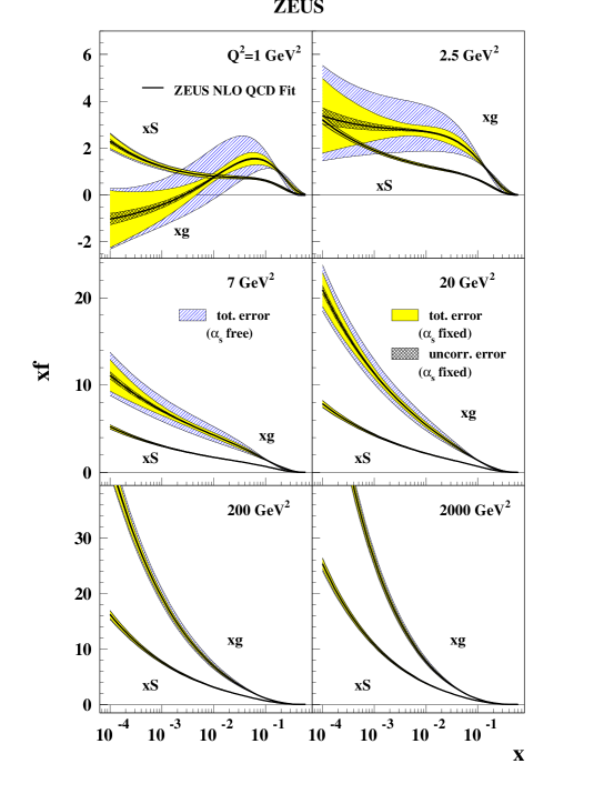
Figure 1: Comparison of the gluon and sea distributions from the ZEUS-S NLO QCD fit for various $Q^{2}$ values. In this figure, the cross-hatched error bands show the statistical and uncorrelated systematic uncertainty, the grey error bands show the total experimental uncertainty including correlated systematic uncertainties (both evaluated from the standard fit with $\alpha_{s}(M_{Z}^{2})=0.118$) and the hatched error bands show the additional uncertainty coming from variation of the strong coupling constant $\alpha_{s}(M_{Z}^{2})$.

These PDFs agree well with the latest distributions from MRST2001 [11] and CTEQ6 [12]. The error bands shown in the figure illustrate the experimental uncertainties from i) statistical and uncorrelated systematic uncertainties alone; ii) total experimental uncertainty including correlated systematic uncertainties; and ii) additional uncertainty due to allowing $\alpha_{s}(M_{Z}^{2})$ to be a parameter of the fit.

Clearly, in the latter case, the fit also determines the value of $\alpha_{s}(M_{Z}^{2})$, with its correlations to the PDF parameters fully accounted. The value

$$\alpha_{s}(M_{Z}^{2})=0.1166\pm 0.0008(\rm uncorr)\pm 0.0032(\rm corr)\pm 0.0036(\rm norm)$$ (2)

is obtained, where the three uncertainties arise from the following: statistical and other uncorrelated sources; correlated systematic sources from all contributing experiments except that from their normalisations; the contribution from the latter normalisations. The contribution from normalisation uncertainties is shown separately from the other systematic uncertainties since, for many experiments, quoted normalisation uncertainties represent the limits of a box-shaped distribution rather than the standard deviation of a Gaussian distribution. An alternative evaluation of normalisation uncertainty, which accounts for this, would reduce this contribution to $\pm 0.0010$.

4.2 Model uncertainties

In addition to the experimental uncertainty on the fitted parameters, there is potentially a model uncertainty due to the specific assumptions made when setting up the NLOQCD fit. Sources of model uncertainty within the theoretical framework of leading-twist NLO QCD are: the effect of varying the value of $Q^{2}_{0}$, and the minimum $Q^{2}$, $x$ and $W^{2}$ of data entering the fit; variation of the form of the input PDF parameterisations; the choice of the heavy-quark production scheme. The sensitivity of the results to the variation of these input assumptions has been quantified in terms of the resulting variation in $\alpha_{s}(M_{Z}^{2})$, since it is the most sensitive parameter. This leads to a model uncertainty in $\alpha_{s}(M_{Z}^{2})$, of $\Delta\alpha_{s}(M_{Z}^{2})\sim\pm 0.0018$, considerably smaller than the errors from correlated systematic and normalisation uncertainties. The PDF parameters are much less sensitive to the model assumptions than $\alpha_{s}(M_{Z}^{2})$. It follows that the error bands illustrated on the parton densities in Fig. 1 represent reasonable estimates of the total uncertainties within the theoretical framework of leading twist NLO QCD.

Sources of uncertainty due to the theoretical framework itself are considered in the contribution of R.Thorne to this meeting.

4.3 Comparison of Offset and Hessian methods

First Hessian method 1 and Hessian method 2 have been compared in a fit to ZEUS data alone, for which the systematic uncertainties and relative normalisations are well understood. The results are very similar, as expected if the systematic uncertainties are Gaussian and the values $\Delta^{sys}_{i\lambda}$ represent one standard deviation uncertainties. However, if data sets from different experiments are used in the fit, these two Hessian methods are only similar if normalisation uncertainties are not included among the systematic uncertainties. Normalisation uncertainties are not always Gaussian and thus the analytic procedure of Hessian method 2 is inappropriate for them.

The offset method has been compared to Hessian method 2 by performing the fit to global DIS data using Hessian method 2 to calculate the $\chi^{2}$. Normalisation uncertainties were excluded and $\alpha_{s}(M_{Z}^{2})$ was included as one of the theoretical parameters. This fit yields, $\alpha_{s}(M_{Z}^{2})=0.1120\pm 0.0013$, where the error represents the total experimental uncertainty from correlated and uncorrelated sources, excluding normalisation uncertainties. Thus this value should be compared with, $\alpha_{s}(M_{Z}^{2})=0.1166\pm 0.0033$, evaluated using the offset method, also excluding normalisation uncertainties (see Eq. 2). Hessian method 2 gives a much reduced ‘optimal’ error estimate for $\alpha_{s}(M_{Z}^{2})$ and this is also the case for the PDF parameters. The value of $\alpha_{s}(M_{Z}^{2})$ is shifted from that obtained by the offset method. The PDF parameters are not affected as strongly, their values are shifted by amounts which are well within the error estimates quoted for the offset method.

To compare the $\chi^{2}$ of the fits done using the offset method and Hessian method 2, it is necessary to use a common method of $\chi^{2}$ calculation. Table 1 presents the $\chi^{2}$ for the theoretical parameters obtained using these methods, re-evaluated by adding statistical and systematic errors in quadrature. For both methods $\alpha_{s}(M_{Z}^{2})$ has been included among the theoretical parameters and normalisation uncertainties have not been included among the systematic parameters. The total increase of $\chi^{2}$ for Hessian method 2 as compared to the offset method is $\Delta\chi^{2}=283$. The results of Hessian method 2 represent a fit with an unacceptably large value of $\chi^{2}$ when judged in this conventional way.

Experiment	data points	$\chi^{2}$/data point	$\chi^{2}$/data point
		Hessian method 2	offset method
ZEUS96/97	242	1.37	0.83
BCDMS p	305	0.95	0.89
NMC p	218	1.50	1.26
NMC D	218	1.15	0.96
E665 D	47	0.97	0.94
E665 p	47	1.17	1.16
CCFRxF3	57	0.99	0.39
NMC D/p	129	0.97	0.93

Table 1: Table of $\chi^{2}$ calculated by adding systematic and statistical errors in quadrature for the theoretical parameters determined by the offset method and Hessian method 2

4.4 Parameter evaluation and Hypothesis Testing

To appreciate the signficance of the difference in $\chi^{2}$ between various fits, the distinction between the $\chi^{2}$ changes appropriate for parameter estimation and for hypothesis testing should be considered. Assuming that the experimental uncertainties which contribute have Gaussian distributions, errors on theoretical parameters which are fitted within a fixed theoretical framework are derived from the criterion for ‘parameter estimation’ $\chi^{2}\to\chi^{2}_{min}+1$. However the goodness of fit of a theoretical hypothesis is judged on ‘hypothesis testing’ criterion, such that its $\chi^{2}$ should be approximately in the range $N\pm\surd(2N)$, where $N$ is the number of degrees of freedom.

Fitting DIS data for PDF parameters and $\alpha_{s}(M_{Z}^{2})$ is not a clean situation of either parameter estimation or hypothesis testing. Within the theoretical framework of leading-twist-NLO QCD, many model inputs such as the form of the PDF parameterisations, the values of cuts, the value of $Q^{2}_{0}$, the data sets used in the fit, etc., can be varied. These represent different hypotheses and they are accepted, provided the fit $\chi^{2}$ fall within the hypothesis-testing criterion. The theoretical parameters obtained for these different model hypotheses can differ from those obtained in the standard fit by more than their errors as evaluated using the parameter-estimation criterion. In this case the model uncertainty on the parameters exceeds the estimate of the total experimental error. This does not happen for the offset method in which the uncorrelated experimental errors evaluated by the parameter estimation criterion are augmented by the contribution of the correlated experimental systematic uncertainties as explained in Section 3. The shifts in theoretical parameter values for the different model hypotheses are found to be well within the total conservative experimental error estimates. However this is no longer the case when the fit is performed using Hessian method 2. In this case the shifts in theoretical parameter values for the different model hypotheses are outside the experimental error estimates. Since our purpose is to estimate errors on the PDF parameters and $\alpha_{s}(M_{Z}^{2})$ within a general theoretical framework, rather than as specific to particular model choices within this framework, this is an issue which must be addressed.

The CTEQ collaboration [10, 12] have considered this problem. They consider that $\chi^{2}\to\chi^{2}+1$ is not a reasonable tolerance on a global fit to $\sim 1200$ data points from diverse sources, with theoretical and model uncertainties which are hard to quantify and experimental uncertainties which may not be Gaussian distributed. They have tried to formulate criteria for a more reasonable setting of the tolerance $T$, such that $\chi^{2}\to\chi^{2}+T^{2}$ becomes the variation on the basis of which errors on parameters are calculated. In setting this tolerance they have considered that all of the current world data sets must be acceptable and compatible at some level, even if strict statistical criteria are not met, since the conditions for the application of strict criteria, namely Gaussian error distributions, are also not met. The level of tolerance they suggest is $T\sim 10$. Note that this is similar to the hypothesis testing tolerance $T=\surd{\surd(2N)}\sim 7$ for the ZEUS fits. The errors for Hessian method 2 have been re-evaluated using the tolerance $T=7$ and, for $\alpha_{s}(M_{Z}^{2})$, the result $\alpha_{s}(M_{Z}^{2})=0.1120\pm 0.0033$ is obtained. The error is now remarkably close to the error estimate of the offset method performed under the same conditions. This is also the case for the errors on all of the PDF parameters.

Thus the offset method and the Hessian method with an augmented tolerance $T=\surd{\surd(2N)}$ give similar conservative error estimates. In choosing between these methods there are some additional considerations.

In the Hessian method it is necessary to check that data points are not shifted far outside their one standard deviation errors. When the ZEUS fits are done by Hessian method 2 some of the systematic shifts for the 10 classes of systematic uncertainty of the ZEUS data move by $\sim\pm 1.4$ standard deviations. There is no single kinematic region responsible for these shifts which could be excluded to reduce this effect. Whereas these shifts are not very large, they differ significantly from the systematic shifts to ZEUS data determined in the CTEQ fit. The choice of data sets included in the ZEUS fit also changes the values of these systematic shifts and making different model assumptions in the fits also produces somewhat different systematic shifts. It seems unreasonable to let variations in the model, or the choice of data included in the fit, change the best estimate of the central value of the data points.

In summary, the offset method has been selected for several reasons. Firstly, because its fit results make theoretical predictions which are as close to the central values of the published data points as possible. The selection of data sets included in the fit or superficial changes to the model are not allowed to change the best estimate of the central value of the data points. Secondly, because its error estimates are equivalent to those of a method which does not assume that experimental systematic uncertainties are Gaussian distributed. Thirdly, because its results produce an acceptable $\chi^{2}$ when re-evaluated conventionally by adding systematic and statistical errors in quadrature. Fourthly, because its conservative error estimates take account of the fact that the purpose is to estimate errors on the PDF parameters and $\alpha_{s}(M_{Z}^{2})$ within a general theoretical framework not specific to particular model choices. Quantitatively the error estimates of the offset method correspond to those which would be obtained using the more generous tolerance of the ‘hypothesis testing’ criterion in the more statistically rigorous Hessian methods.

5 CONCLUSION

The NLO DGLAP QCD formalism has been used to fit ZEUS data and fixed-target data in the kinematic region, $Q^{2}>2.5$GeV², $6.3\times 10^{-5}<x<0.65$ and $W^{2}>20$GeV². The parton distribution functions for the $u$ and $d$ valence quarks, the gluon and the total sea have been determined and the results are compatible with those of MRST2001 and CTEQ6. The ZEUS data are crucial in determining the gluon and the sea distributions.

Full account has been taken of correlated experimental systematic uncertainties for all experiments. The resulting experimental uncertainties on the parton distribution functions have been evaluated conservatively, such that the model uncertainty, within the framework of leading-twist next-to-leading-order QCD, is negligible by comparison. Hence the error bands on the PDFs resulting from these fits represent reasonable estimates of the total uncertainties within this theoretical framework.

References

- [1] V.N. Gribov and L.N. Lipatov, Sov. J. Nucl. Phys 15 (1972) 438, L.N. Lipatov, Sov. J. Nucl. Phys 20 (1975) 94, G. Altarelli and G. Parisi, Nucl. Phys. B126 (1977) 298, Yu.L. Dokshitzer, Sov. Phys. JETP 46 (1977) 641.
- [2] ZEUS Coll., S. Chekanov et al., forthcoming.
- [3] ZEUS Coll., S. Chekanov et al., Eur. Phys. J. C21 (2001) 443.
- [4] HEPDATA, http://durpdg.durham.ac.uk/HEPDATA
- [5] R.S.Thorne and R.G.Roberts, Phys. Rev. D57 (1998) 6871.
- [6] Particle Data Group, D.E Groom et al., Eur. Phys. J. C15 (2000) 1.
- [7] C. Pascaud and F. Zomer, Preprint LAL-95-05.
- [8] M. Botje, hep-ph/0110123.
- [9] S.I. Alekhin, hep-ex/0005042.
- [10] CTEQ Coll., J. Stump et al., Phys. Rev. D65 (2001) 014012, J. Pumplin et al., Phys. Rev. D65 (2001) 014013.
- [11] A.D. Martin et al., hep-ph/0110215
- [12] J. Pumplin et al., hep-ph/0201195