Constraint on the CKM angle $\alpha$ from the experimental measurements of CP violation in $B_{d}^{0}\to\pi^{+}\pi^{-}$ decay

Abstract

In this paper, we study and try to find the constraint on the CKM angle $\alpha$ from the experimental measurements of CP violation in $B_{d}^{0}\to\pi^{+}\pi^{-}$ decay, as reported very recently by BaBar and Belle Collaborations. After considering uncertainties of the data and the ratio $r$ of penguin over tree amplitude, we found that strong constraint on both the CKM angle $\alpha$ and the strong phase $\delta$ can be obtained from the measured CP asymmetries $S_{\pi\pi}$ and $A_{\pi\pi}$: (a) the ranges of $87^{\circ}\leq\alpha\leq 131^{\circ}$ and $36^{\circ}\leq\delta\leq 144^{\circ}$ are allowed by $1\sigma$ of the averaged data for $r=0.31$; (b) for Belle’s result alone, the limits on $\alpha$ and $\delta$ are $104^{\circ}\leq\alpha\leq 139^{\circ}$ and $42^{\circ}\leq\delta\leq 138^{\circ}$ for $0.32\leq r\leq 0.41$; and (c) the angle $\alpha$ larger than $90^{\circ}$ is preferred.

I Introduction

To study CP violation mechanism is one of the main goals of the B factory experiments. In the standard model (SM), the CP violation is induced by the nonzero phase angle appeared in the Cabbibo-Kobayashi-Maskawa (CKM) mixing matrix. Recent measurements of $\sin{2\beta}$ in neutral B meson decay $B_{d}^{0}\to J/\psi K_{S,L}^{0}$ by BABAR [1, 2] and Belle [3, 4] Collaborations established the third type CP violation (interference between the decay and mixing ) of $B_{d}$ meson system. Two new measurements of $\sin{2\beta}$ as reported this year by BaBar [2] and Belle [5] Collaborations are

$$\sin{(2\beta)} = 0.75\pm 0.09(stat.)\pm 0.04(syst.),$$ (1)

$$\sin{(2\beta)} = 0.82\pm 0.12(stat.)\pm 0.05(syst.),$$ (2)

with an average

$$\sin{(2\beta)}=0.78\pm 0.08,$$ (3)

which is well consistent with last year’s world average, $\sin{(2\beta)}=0.79\pm 0.10$, and leads to the bounds on the angle $\beta$:

$$\beta=\left(26^{\circ}\pm 4^{\circ}\right)\bigvee\left(64^{\circ}\pm 4^{\circ}\right).$$ (4)

Despite the well measured CKM angle $\beta$, we have very poor knowledge on the other two angles $\alpha$ and $\gamma$. Very recently, Belle collaboration reported their first measurements of the CP violation of the $B_{d}^{0}\to\pi^{+}\pi^{-}$ decay [5]:

$$S_{\pi\pi} = -1.21^{+0.38}_{-0.27}(stat.)^{+0.16}_{-0.13}(syst.),$$ (5)

$$A_{\pi\pi} = +0.94^{+0.25}_{-0.31}(stat.)\pm 0.09(syst).$$ (6)

The probability for $S_{\pi\pi}\neq 0$ and $A_{\pi\pi}\neq 0$ is $99.9\%$ [5]. Based on a data sample of about $88$ million $\Upsilon(4S)\to B\bar{B}$ decays, the BaBar Collaboration updated their measurement of CP violating asymmetries of $B\to\pi^{+}\pi^{-}$ decay [6]

$$S_{\pi\pi} = 0.02\pm 0.34(stat.)\pm 0.05(syst.),$$ (7)

$$C_{\pi\pi} = -0.30\pm 0.25(stat.)\pm 0.04(syst.).$$ (8)

The uncertainties of BABAR’s new results are smaller than those of their previous results[7, 8]. It is easy to see that the experimental measurements of BABAR and Belle collaborations are not fully consistent with each other: BABAR’s results are still consistent with zero, while the Bells’s results strongly indicate nonzero $S_{\pi\pi}$ and $A_{\pi\pi}$. Further improvement of the data will enable us to draw definite conclusions about the values of both $S_{\pi\pi}$ and $A_{\pi\pi}$.

Inspired by the recent measurements, discussions have been made to obtain information on strong phases and CKM phases from the recent experimental measurements [9, 10]. In Ref.[9], Gronau and Rosner examined the time-dependent measurements of $B\to\pi^{+}\pi^{-}$ decay to draw information on strong and weak phases and found that: (a) if $\sin{\delta}$ is small a discrete ambiguity between $\delta\simeq 0$ and $\delta\simeq\pi$ could be resolved by comparing the measured branching ratio $Br(B\to\pi^{+}\pi^{-})$ with that predicted in the absence of the penguin amplitude; (b) if $A_{\pi\pi}$ is non-zero, the discrete ambiguity between $\delta$ and $\pi-\delta$ becomes harder to resolve, but its effects on CKM parameters becomes less important, and (c) the sign of the quantity $D_{\pi\pi}=2Re(\lambda_{\pi\pi})/(1+|\lambda_{\pi\pi}|^{2})$ is always negative for the allowed range of CKM parameters and therefore a positive value of $D_{\pi\pi}$ would signify new physics beyond the SM. In Ref.[10], Fleischer and Matias investigated the allowed regions in observable space of $B\to\pi K$, $B_{d}\to\pi^{+}\pi^{-}$ and $B_{s}\to K^{+}K^{-}$ decays. They considered the correlations between these three kinds of decay modes implied by the SU(3) flavor symmetry and the U-spin symmetry and found the new constraint on the CKM angle $\gamma$ by using the B-factory measurements of CP violation of $B_{d}\to\pi^{+}\pi^{-}$.

As it is well-known that, the CP asymmetry measurements in $B\to\pi\pi$ decays play an important role in extracting out the CKM angle $\alpha$. In this paper, we focus on the $B\to\pi^{+}\pi^{-}$ decay and try to extract out the constraint on the angle $\alpha$ from the measured $S_{\pi\pi}$ and $A_{\pi\pi}$ and the ratio $r$ of penguin over tree amplitude fixed by theoretical argument. Taking into account both Belle and BABAR newest measurements[5, 6], the weighted-averages of $S_{\pi\pi}$ and $A_{\pi\pi}$ are

$$S_{\pi\pi}^{exp}=-0.57\pm 0.25,\ \ A_{\pi\pi}^{exp}=0.57\pm 0.19.$$ (9)

We will treat above averages as the measured asymmetries of $B_{d}\to\pi^{+}\pi^{-}$ decay in the following analysis. We also investigate what will happen if only Bells’s measurements are taken into account. For the case of $S_{\pi\pi}\approx 0$ and $A_{\pi\pi}\approx 0$ as indicated by BABAR’s results alone, one can see the discussions given in Ref.[9].

This paper is organized as follows. In Sec. II we present the general description of CP asymmetries of the $B\to\pi^{+}\pi^{-}$ decay. In Sec. III we consider the new Babar and Belle’s measurements of $S_{\pi\pi}$ and $A_{\pi\pi}$ to draw the constraints on the CKM angle $\alpha$ and the strong phase $\delta$. The conclusions are included in the final section.

II CP asymmetries of $B\to\pi^{+}\pi^{-}$ decay

In the SM with SU(2)$\times$U(1) as the gauge group, the quark mass eigenstates are not the same as the weak eigenstates. The mixing between (down type) quark mass eigenstates was described by the CKM matrix [11]. The mixing is expressed in terms of a $3\times 3$ unitary matrix $V_{CKM}$ operating on the down type quark mass eigenstates (d,s, and b):

$$\left(\begin{array}[]{ccc}d^{\prime}\\ s^{\prime}\\ b^{\prime}\end{array}\right)=\left(\begin{array}[]{ccc}V_{ud}&V_{us}&V_{ub}\\ V_{cd}&V_{cs}&V_{cb}\\ V_{td}&V_{ts}&V_{tb}\end{array}\right)\left(\begin{array}[]{ccc}d\\ s\\ b\end{array}\right).$$ (10)

As a $3\times 3$ unitary matrix, the CKM mixing matrix $V_{CKM}$ is fixed by four parameters, one of which is an irreducible complex phase. Using the generalized Wolfenstein parametrization[12], $V_{CKM}$ takes the form

$$V_{CKM}=\left(\begin{array}[]{ccc}1-\frac{\lambda^{2}}{2}&\lambda&A\lambda^{3}(\bar{\rho}-i\bar{\eta})\\ -\lambda&1-\frac{\lambda^{2}}{2}&A\lambda^{2}\\ A\lambda^{3}(1-\bar{\rho}-i\bar{\eta})&-A\lambda^{2}&1\end{array}\right).$$ (11)

where $A$, $\lambda$, $\bar{\rho}$ and $\bar{\eta}$ are Wolfenstein parameters.

The unitarity of the CKM matrix implies six “unitarity triangle”. One of them applied to the first and third columns of the CKM matrix yields

$$V_{ud}V_{ub}^{*}+V_{cd}V_{cb}^{*}+V_{td}V_{tb}^{*}=0.$$ (12)

This unitary triangle is just a geometrical presentation of this equation in the complex plane. We show it in the $\bar{\rho}-\bar{\eta}$ plane, as illustrated in Fig.1.

The three unitarity angles are defined as

$$\alpha = \arg\left(-\frac{V_{tb}^{*}V_{td}}{V_{ub}^{*}V_{ud}}\right),$$ (13)

$$\beta = \arg\left(-\frac{V_{cb}^{*}V_{cd}}{V_{tb}^{*}V_{td}}\right),$$ (14)

$$\gamma = \arg\left(-\frac{V_{ub}^{*}V_{ud}}{V_{cb}^{*}V_{cd}}\right).$$ (15)

The above definitions are independent of any kind of parametrization of the CKM matrix elements. Thus it is universal. In the Wolfenstein parametrization, in terms of $(\bar{\rho},\bar{\eta})$, $\sin(2\phi_{i})$ ($\phi_{i}=\alpha,\beta,\gamma$) can be written as

$$\sin(2\alpha) = \frac{2\bar{\eta}(\bar{\eta}^{2}+\bar{\rho}^{2}-\bar{\rho})}{(\bar{\rho}^{2}+\bar{\eta}^{2})((1-\bar{\rho})^{2}+\bar{\eta}^{2})},$$ (16)

$$\sin(2\beta) = \frac{2\bar{\eta}(1-\bar{\rho})}{(1-\bar{\varrho})^{2}+\bar{\eta}^{2}},$$ (17)

$$\sin(2\gamma) = \frac{2\bar{\rho}\bar{\eta}}{\bar{\rho}^{2}+\bar{\eta}^{2}}.$$ (18)

The SM predicts the CP-violating asymmetries in the time-dependent rates for initial $B^{0}$ and $\bar{B}^{0}$ decays to a common CP eigenstate $f_{CP}$. In the case of $f_{CP}=\pi^{+}\pi^{-}$, the time-dependent rate is given by

$$f_{\pi\pi}(\Delta t)=\frac{e^{-|\Delta t|/\tau_{B^{0}}}}{4\tau_{B^{0}}}\left\{1+q\cdot\left[S_{\pi\pi}\sin{(\Delta m_{d}\Delta t)}+A_{\pi\pi}\cos{(\Delta m_{d}\Delta t)}\right]\right\},$$ (19)

where $\tau_{B^{0}}$ is the $B_{d}^{0}$ lifetime, $\Delta m_{d}$ is the mass difference between the two $B_{d}^{0}$ mass eigenstates, $\Delta t=t_{CP}-t_{tag}$ is the time difference between the tagged-$B^{0}$ ($\bar{B}^{0}$) and the accompanying $\bar{B}^{0}$ ( $B^{0}$) with opposite $b-$flavor decaying to $\pi^{+}\pi^{-}$ at the time $t_{CP}$, $q=+1$ ($-1$) when the tagging $B$ meson is a $B^{0}$ ($\bar{B}^{0}$). The CP-violating asymmetries $S_{\pi\pi}$ and $A_{\pi\pi}$ have been defined as

$$S_{\pi\pi}=\frac{2{\rm Im}\,(\lambda_{\pi\pi})}{1+|\lambda_{\pi\pi}|^{2}},\ \ A_{\pi\pi} = \frac{|\lambda_{\pi\pi}|^{2}-1}{1+|\lambda_{\pi\pi}|^{2}},$$ (20)

where the parameter $\lambda_{\pi\pi}$ is

$$\lambda_{\pi\pi} = \frac{V_{tb}^{*}V_{td}}{V_{tb}V_{td}^{*}}\left[\frac{V_{ub}V_{ud}^{*}T_{\pi\pi}e^{i\delta_{1}}-V_{tb}V_{td}^{*}P_{\pi\pi}e^{i\delta_{2}}}{V_{ub}^{*}V_{ud}T_{\pi\pi}e^{i\delta_{1}}-V_{tb}^{*}V_{td}PP_{\pi\pi}e^{i\delta_{2}}}\right]$$ (21)

$$= e^{2i\alpha}\left[\frac{1+re^{i(\delta-\alpha)}}{1+re^{i(\delta+\alpha)}}\right],$$ (22)

with

$$r=\left|\frac{P_{\pi\pi}}{T_{\pi\pi}}\right|\left|\frac{V_{tb}V_{td}^{*}}{V_{ub}V_{ud}^{*}}\right|,\ \ \delta=\delta_{2}-\delta_{1},$$ (23)

where $T_{\pi\pi}$ and $P_{\pi\pi}$ describe the “Tree” and penguin contributions to the $B_{d}^{0}\to\pi^{+}\pi^{-}$ decay, and $\delta$ is the difference of the corresponding strong phases of tree and penguin amplitudes.

By explicit calculations, we find that

$$S_{\pi\pi} = \frac{\sin{2\alpha}+2r\cos{\delta}\sin{\alpha}}{1+r^{2}+2r\cos{\delta}\cos{\alpha}},$$ (24)

$$A_{\pi\pi} = \frac{2r\sin{\delta}\sin{\alpha}}{1+r^{2}+2r\cos{\delta}\cos{\alpha}}.$$ (25)

If we neglect the penguin-diagram (which is expected to be smaller than the tree diagram contribution), we have $A_{\pi\pi}=0$, $S_{\pi\pi}=\sin(2\alpha)$. That means we can measure the $\sin(2\alpha)$ directly from $B_{d}^{0}\to\pi^{+}\pi^{-}$ decay. This is the reason why $B_{d}^{0}\to\pi^{+}\pi^{-}$ decay was assumed to be the best channel to measure CKM angle $\alpha$ previously. With penguin contributions, we have $A_{\pi\pi}\neq 0,S_{\pi\pi}=\sin(2\alpha_{eff})$, where $\alpha_{eff}$ depends on the magnitude and strong phases of the tree and penguin amplitudes. In this case, the CP asymmetries can not tell the size of angle $\alpha$ directly. A method has been proposed to extract CKM angle $\alpha$ using $B^{+}\to\pi^{+}\pi^{0}$ and $B^{0}\to\pi^{0}\pi^{0}$ decays together with $B_{d}^{0}\to\pi^{+}\pi^{-}$ decay by the isospin relation [13]. However, it will take quite some time for the experiments to measure the three channels together.

III Constraint on $\alpha$ and $\delta$

In this section, we will show that the only measured CP asymmetries of $B_{d}^{0}\to\pi^{+}\pi^{-}$ decay can at least provide some constraint on the angle $\alpha$.

From Eq.(24,25), one can see that the asymmetries $S_{\pi\pi}$ and $A_{\pi\pi}$ generally depend on three “free” parameters: the CKM angle $\alpha$ with $\alpha=[0,\pi]$, the strong phase $\delta$ with $\delta=[-\pi,\pi]$ and the ratio $r$ as defined in Eq.(23). We can not solve out these two equations with three unknown variables. However, by the following study, we can at least give some constraint on the angle $\alpha$ and strong phase $\delta$. Since the penguin contributions are loop order corrections ($\alpha_{s}$ suppressed) comparing with the tree contribution, we can assume $0<r<0.5$, in a reasonable range.

Now we are ready to extract out $\alpha$ through the general parameterization of $S_{\pi\pi}$ and $A_{\pi\pi}$ in terms of $(\alpha,\delta,r)$ as given in Eqs.(24,25). As discussed previously [9], there may exist some discrete ambiguities between $\delta$ and $\pi-\delta$ for the mapping of $S_{\pi\pi}$ and $A_{\pi\pi}$ onto the $\delta-\alpha$ plane.

At first, because of the positiveness of $A_{\pi\pi}^{exp}$ at $1\sigma$ level and the fact that $\sin{\alpha}>0$ for $\alpha=(0,\pi)$, the range of $-\pi<\delta<0$ and $\delta=0,\pm\pi$ are excluded. and therefore only the range of $0^{\circ}<\delta<180^{\circ}$ need to be considered here.

For the special case of $\delta=90^{\circ}$, the discrete ambiguity between $\delta$ and $\pi-\delta$ disappear and the expressions of $S_{\pi\pi}$ and $A_{\pi\pi}$ can be rewritten as

$$S_{\pi\pi} = \frac{\sin{2\alpha}}{1+r^{2}},$$ (26)

$$A_{\pi\pi} = \frac{2r\sin{\alpha}}{1+r^{2}}.$$ (27)

The range of $0^{\circ}\leq\alpha\leq 90^{\circ}$ is excluded by the negativeness of $S_{\pi\pi}^{exp}$, and the range of $\sin{\alpha}<0.19(1+r^{2})/r$ and $\sin{\alpha}>0.38(1+r^{2})/r$ are excluded by the measured $A_{\pi\pi}=0.57\pm 0.19$ at the $1\sigma$ level.

In Fig.2a, we show the $\alpha$ dependence of $S_{\pi\pi}$ for given $\delta=90^{\circ}$ and for $r=0.1$ (dotted curve), $0.2$ (tiny-dashed curve), $0.3$ (solid curve), $0.4$ (dashed curve) and $0.5$ (dash-dotted curve), respectively. The band between the two horizontal dots lines shows the allowed range from the measured $S_{\pi\pi}^{exp}=-0.57\pm 0.25$ at $1\sigma$ level. Fig.2b shows the $\alpha$ dependence of $S_{\pi\pi}$ for fixed $r=0.3$ and for $\delta=30^{\circ}$ (dotted curve),$60^{\circ}$ (tiny-dashed curve), $90^{\circ}$ (solid curve), $120^{\circ}$ (dashed curve), and $150^{\circ}$ (dash-dotted curve), respectively. The differences between the curves of $\delta=30^{\circ}$ and $\delta=150^{\circ}$ ( $\delta=60^{\circ}$ and $\delta=120^{\circ}$) show the effects of discrete ambiguity between $\delta$ and $\pi-\delta$.

The constraint on the CKM angle $\alpha$ from the measured $S_{\pi\pi}$ alone can be read off directly from figure 2. For $r=0.3$, for example, the allowed ranges for the CKM angle $\alpha$ are

$$109^{\circ}\leq\alpha\leq 128^{\circ}\bigvee 153^{\circ}\leq\alpha\leq 171^{\circ}$$ (28)

for $\delta=60^{\circ}$, and

$$101^{\circ}\leq\alpha\leq 121^{\circ}\bigvee 149^{\circ}\leq\alpha\leq 169^{\circ}$$ (29)

for $\delta=90^{\circ}$, and

$$92^{\circ}\leq\alpha\leq 112^{\circ}\bigvee 146^{\circ}\leq\alpha\leq 168^{\circ}$$ (30)

for $\delta=120^{\circ}$. In general, the current experimental measurements of $S_{\pi\pi}$ prefer to $\alpha>90^{\circ}$.

In Fig.3a, we show the $\alpha$ dependence of $A_{\pi\pi}$ for given $\delta=90^{\circ}$ and $r=0.1$ (dotted curve), $0.2$ (tiny-dashed curve), $0.3$ (solid curve), $0.4$ (dashed curve) and $0.5$ (dash-dotted curve), respectively. The band between two horizontal dots line shows the allowed region by the measured $A_{\pi\pi}^{exp}=0.57\pm 0.19$ at $1\sigma$ level. Fig.3b shows the $\alpha$ dependence of $A_{\pi\pi}$ for given $r=0.3$ and for $\delta=30^{\circ}$ (dotted curve),$60^{\circ}$ (tiny-dashed curve), $90^{\circ}$ (solid curve), $120^{\circ}$ (dashed curve), and $150^{\circ}$ (dash-dotted curve), respectively. It is easy to see that most parts of the allowed ranges of $\alpha$ as given in Eqs.(28-30) can be excluded by the inclusion of measured $A_{\pi\pi}$. The second solutions as given in Eqs.(28-30) will be removed by taking the measured $A_{\pi\pi}$ into account. For the case of $r=0.3$ and $\delta\leq 30^{\circ}$ or $\delta\geq 150^{\circ}$, the whole range of $\alpha$ will be excluded by the measured $S_{\pi\pi}$ and $A_{\pi\pi}$, as illustrated in Fig.3b.

From the above analysis, we can see that the strong constraint on CKM angle $\alpha$ can be obtained by using the experimental measurements of $S_{\pi\pi}$ and $A_{\pi\pi}$ as well as the ratio $r$. With the rapid increase of the $B\bar{B}$ pair production and decay events collected at B-factory experiments, the difference between the central value of $S_{\pi\pi}$ and $A_{\pi\pi}$ and the experimental uncertainties will become smaller within two years. For the third input parameter $r$, it can be fixed through available data or reliable theoretical considerations.

From Eqs.(3) and (17), the measured $\sin{(2\beta)}$ leads to an equation between $\bar{\rho}$ and $\bar{\eta}$,

$$\bar{\eta}=(1-\bar{\rho})\xi=(1-\bar{\rho})\frac{1\pm\sqrt{1-\sin^{2}(2\beta)}}{\sin{(2\beta)}}.$$ (31)

The solution with the $``+"$ sign in the numerator of $\xi$ is totally inconsistent with the global fit results and can be dropped out. Numerically,

$$\xi=\left(1-\sqrt{1-\sin^{2}(2\beta)}\right)/\sin{(2\beta)}=0.48^{+0.09}_{-0.07},$$ (32)

for the measured $\sin{(2\beta)}=0.78\pm 0.08$. There exist quite a lot of information about the CKM matrix elements as reported by the Particle Data Group [15] and other recent papers [14, 16, 17, 18, 19]. The parameter $\lambda=|V_{us}|$ is known from $K_{l3}$ decay with good precision

$$\lambda=0.2196\pm 0.0023.$$ (33)

In terms of $(\bar{\rho},\bar{\eta})$, the parameter $r$ as defined in Eq.(23) can be rewritten as

$$r = z\frac{\sqrt{(1-\bar{\rho})^{2}+\bar{\eta}^{2}}}{\sqrt{\bar{\rho}^{2}+\bar{\eta}^{2}}\left(1-\frac{\lambda^{2}}{2}\right)}=\frac{z}{1-\frac{\lambda^{2}}{2}}\frac{(1-\bar{\rho})\sqrt{1+\xi^{2}}}{\sqrt{\bar{\rho}^{2}+(1-\bar{\rho})^{2}\xi^{2}}},$$ (34)

where $z=|P_{\pi\pi}/T_{\pi\pi}|$ measures the relative size of tree and penguin contribution to the studied decay. From general considerations, $z$ may be around $20\%$. By employing the QCD factorization approach [20] and/or the perturbative QCD approach [21], one can fix $r$ to a rather good degree. By using the QCD factorization approach, the estimated value of $|P_{\pi\pi}/T_{\pi\pi}|$ is found [20] to be

$$z=0.285\pm 0.077,$$ (35)

where the contribution from the weak annihilation has been taken into account and the dominate error comes from the uncertainties of $m_{s}$ and the renormalization scale $\mu$ [20]. From the numbers as given in Eqs.(32,33,35) and $\bar{\rho}=0.20\pm 0.16$, we have numerically

$$r=0.31\pm 0.09(\Delta z)\pm 0.01(\Delta\xi)^{+0.01}_{-0.03}(\Delta\bar{\rho})\pm 0.0002(\Delta\lambda)=0.31\pm 0.10,$$ (36)

Here the estimated result $r\leq 0.41$ is in good agreement with our general argument of $r<0.5$. Thus our analysis in this paper is meaningful.

The common range of $\alpha$ allowed by both the measured $S_{\pi\pi}$ and $A_{\pi\pi}$ is what we try to find. Fig.4 shows the contour plots of the CP asymmetries $S_{\pi\pi}$ and $A_{\pi\pi}$ versus the strong phase $\delta$ and CKM angle $\alpha$ for $r=0.21$ (the small circles in (a)), $0.31$ (the larger circles in (a)) and $0.41$ (circles in (b)), respectively. The regions inside each circle are still allowed by both $S_{\pi\pi}^{exp}=-0.57\pm 0.25$ and $A_{\pi\pi}^{exp}=0.57\pm 0.19$ (experimental $1\sigma$ allowed ranges). The discrete ambiguity between $\delta$ and $\pi-\delta$ are shown by the solid and dotted circles in Fig.4. For $\delta=90^{\circ}$, such discrete ambiguity disappear.

If we take the theoretically fixed value of $r=0.31\pm 0.10$ as the reliable estimation of $r$, the constraint on the CKM angle $\alpha$ and the strong phase $\delta$ can be read off directly from Fig.4. Numerically, the allowed regions for the CKM angle $\alpha$ and the strong phase $\delta$ are

$$97^{\circ}\leq\alpha\leq 113^{\circ},\ \ 68^{\circ}\leq\delta\leq 112^{\circ}$$ (37)

for $r=0.21$, and

$$87^{\circ}\leq\alpha\leq 131^{\circ},\ \ 36^{\circ}\leq\delta\leq 144^{\circ}$$ (38)

for $r=0.31$, and finally

$$80^{\circ}\leq\alpha\leq 138^{\circ}\bigvee 143^{\circ}\leq\alpha\leq 155^{\circ},$$ (39)

$$24^{\circ}\leq\delta\leq 151^{\circ}$$ (40)

for $r=0.41$. There is a twofold ambiguity for the determination of angle $\alpha$ for $r\approx 0.4$. In fact, the CKM angle $\alpha$ in the second region in Eq.(40) is too big to be consistent with the standard model unitarity relation: $\alpha+\beta+\gamma=180^{\circ}$.

One can see from Fig.4 that if we take the weighted-average of the BaBar and Belle first measurements of the asymmetries $S_{\pi\pi}$ and $A_{\pi\pi}$ as the reliable measured values of $S_{\pi\pi}$ and $A_{\pi\pi}$, we can obtain strong constraint on both the strong phase $\delta$ and the CKM angle $\alpha$. Even we consider the uncertainties of input parameters, most part of the parameter space is also excluded.

In order to show more details of the $r$ dependence of the constraint on $\alpha$, we draw Fig.5. The semi-closed regions as shown in Fig.5a (for $\delta=60^{\circ}$ and $120^{\circ}$) and Fig.5b (for $\delta=90^{\circ}$) are still allowed by the measured $S_{\pi\pi}$ and $A_{\pi\pi}$ as given in Eq.(9). As shown in Fig.5, the region of $r\leq 0.2$ is excluded by the data. The effects of discrete ambiguity are also shown in Fig.5. The solid semi-closed region in Fig.5a corresponds to $\delta=60^{\circ}$, while the dotted semi-closed region refers to $\pi-\delta=120^{\circ}$. For $\delta=90^{\circ}$, such discrete ambiguity disappears.

As discussed in previous section, there are some discrepancy between the BABAR and Belle measurements of $S_{\pi\pi}$ and $A_{\pi\pi}$ (or $C_{\pi\pi}$ ). If we use Belle’s measurement of $S_{\pi\pi}$ and $A_{\pi\pi}$ only, and take the direct sum of statistic and systematic errors as the total $1\sigma$ error, then the experimental limits on both $S_{\pi\pi}$ and $A_{\pi\pi}$ take the form

$$S_{\pi\pi}^{exp}\leq-0.67,\ \ A_{\pi\pi}^{exp}\geq 0.54.$$ (41)

The corresponding contour plots of the asymmetries $S_{\pi\pi}$ and $A_{\pi\pi}$ versus the strong phase $\delta$ and CKM angle $\alpha$ are illustrated in Fig.6 for $r=0.36$ (the small solid circle), $0.41$ (the middle-sized solid circle) and $0.51$ (the large solid circle), respectively. For $r\leq 0.32$, the whole $``\delta-\alpha"$ plane is excluded. The dotted circles correspond to the discrete ambiguity between $\delta$ and $\pi=\delta$. Numerically, we find that the allowed ranges for the CKM angle $\alpha$ and the strong phase $\delta$ are

$$108^{\circ}\leq\alpha\leq 130^{\circ},\ \ 54^{\circ}\leq\delta\leq 126^{\circ}$$ (42)

for $r=0.36$, and

$$104^{\circ}\leq\alpha\leq 139^{\circ},\ \ 42^{\circ}\leq\delta\leq 138^{\circ}$$ (43)

for $r=0.41$, and finally

$$95^{\circ}\leq\alpha\leq 152^{\circ},\ \ 28^{\circ}\leq\delta\leq 152^{\circ}$$ (44)

for $r=0.51$, although we do not expect so large value of the ratio $r$.

If we use the Belle’s measurement of $S_{\pi\pi}$ and $A_{\pi\pi}$ only, and take the square root of the statistic and systematic errors as the total $1\sigma$ error, then the experimental limits on both $S_{\pi\pi}$ and $A_{\pi\pi}$ will be

$$S_{\pi\pi}^{exp}\leq-0.80,\ \ A_{\pi\pi}^{exp}\geq 0.62.$$ (45)

The whole $``\delta-\alpha"$ plane will be excluded even for $r=0.51$. In other word, the Belle result has to be changed in the future, otherwise, new physics may be required to explain the data.

Since the discrete ambiguity between $\delta$ and $\pi-\delta$ vanishes when $\delta=\pi/2$, the contour plots as shown in Figs.4 and 6 are symmetric with respect to the axis of $\delta=90^{\circ}$ in the $\delta-\alpha$ plane. Such discrete ambiguity can alter the constraints on $\delta$ by about $7^{\circ}$, but has little effect on the possible limits on the CKM angle $\alpha$ derived from the measured $S_{\pi\pi}$ and $A_{\pi\pi}$ if we fix the value of $r$ and treat $\delta$ as a free parameter varying in the range of $0^{\circ}<\delta<180^{\circ}$ as can be seen in Figs. 4 and 6.

It is worth to mention that the constraint on the angle $\alpha$ from one recent global fit is $82^{\circ}\leq\alpha\leq 126^{\circ}$ as given in Ref.[14]. The constraint from measured $S_{\pi\pi}$ and $A_{\pi\pi}$ is comparable or stronger than the global fit result.

IV Conclusion

In this paper, we studied the $B_{d}^{0}\to\pi^{+}\pi^{-}$ decay and try to find constraint on the CKM angle $\alpha$ and the strong phase $\delta$ from the measured asymmetries $S_{\pi\pi}$ and $A_{\pi\pi}$ as reported by the BaBar and Belle Collaborations.

If we take the weighted-average of BABAR and Belle’s measurements of $S_{\pi\pi}$ and $A_{\pi\pi}$ as the measured results, strong constraint on both the CKM angle $\alpha$ and the strong phase $\delta$ can be obtained. The range of $\delta\leq 0$ is excluded by the positiveness of measured $A_{\pi\pi}$. The range of $0^{\circ}\leq\alpha\leq 90^{\circ}$ is excluded by the negativeness of measured $A_{\pi\pi}$ for $\delta=90^{\circ}$. Within the parameter space of $S_{\pi\pi}=-0.57\pm 0.25$, $A_{\pi\pi}=0.57\pm 0.19$ and $r=0.31\pm 0.10$, most part of the $``\delta-\alpha"$ plane is excluded, as shown in Figs.(3-6). For fixed $r=0.31$, for example, the ranges of $87^{\circ}\leq\alpha\leq 131^{\circ}$ and $36^{\circ}\leq\delta\leq 144^{\circ}$ are allowed by $1\sigma$ of the averaged $S_{\pi\pi}$ and $A_{\pi\pi}$. In general the data prefer $\alpha>90^{\circ}$.

The discrete ambiguity between $\delta$ and $\pi-\delta$ will disappear for $\delta=90^{\circ}$ and has little effects on the possible limits on the CKM angle $\alpha$ if we fix the value of $r$ and treat $\delta$ as a free parameter varying in the range of $0^{\circ}<\delta<180^{\circ}$, as shown in Figs. 4 and 6.

If we consider only Belle’s measurements, a very narrow range in the $``\delta-\alpha"$ plane is allowed, as illustrated in Fig.6. The limits on $\alpha$ and $\delta$ are $104^{\circ}\leq\alpha\leq 139^{\circ}$ and $42^{\circ}\leq\delta\leq 138^{\circ}$ for $0.32\leq r\leq 0.41$; Considering the previous $\sin 2\beta$ measurement $\beta=26^{\circ}\pm 4^{\circ}$), we can conclude that the other CKM angle $\gamma$ should be smaller than $90^{\circ}$.

We know that the current data of $S_{\pi\pi}$ and $A_{\pi\pi}$ are still some kind of preliminary experimental measurements with large uncertainties. The apparent large difference between the BABAR and Belle measurements and the corresponding experimental uncertainties will become smaller along with the rapid increase of the observed $B$ decay events. Therefore we are able to extract out the angle $\alpha$ with a good accuracy soon.

FIG. 1.: Unitarity triangle in $\bar{\rho},\bar{\eta}$ plane.

FIG. 2.: Plots of $S_{\pi\pi}$ vs the angle $\alpha$. (a) The dots-, tiny dashed-, solid-, dashed and dash-dotted curves correspond to $r=0.1$, $r=0.2$, $0.3$ $r=0.4$ and $0.5$, respectively. (b) The five curves from left to right are for $\delta=150^{\circ},120^{\circ}$, $90^{\circ}$, $60^{\circ}$ and $30^{\circ}$ respectively. The band between two horizontal dotted lines shows the experimental $1\sigma$ allowed range $-0.82\leq S_{\pi\pi}^{exp}\leq-0.32$.

FIG. 3.: Plots of $A_{\pi\pi}$ vs the angle $\alpha$. In (a) the dots-, tiny dashed-, solid-, dashed and dash-dotted curves correspond to $r=0.1$, $0.2$, $0.3$ $0.4$ and $0.5$, respectively. In (b) the same ordered curves are for $\delta=30^{\circ}$, $\delta=60^{\circ}$, $\delta=90^{\circ}$, $130^{\circ}$ and $150^{\circ}$ respectively. The band between two horizontal dotted lines shows the experimental $1\sigma$ allowed range $0.38\leq A_{\pi\pi}^{exp}\leq 0.76$.

FIG. 4.: Contour plots of the asymmetries $S_{\pi\pi}$ and $A_{\pi\pi}$ versus the strong phase $\delta$ and CKM angle $\alpha$ for $r=0.21$ (the small circles in (a)) and $0.31$ (the large circles in (a)), and $0.41$ (b), respectively. The dotted circles show the effects of discrete ambiguity. The regions inside each circle are still allowed by both $-0.82\leq S_{\pi\pi}^{exp}\leq-0.32$ and $0.38\leq A_{\pi\pi}^{exp}\leq 0.76$, which is the experimental $1\sigma$ allowed range.

FIG. 5.: Contour plots of the asymmetries $S_{\pi\pi}$ and $A_{\pi\pi}$ versus the CKM angle $\alpha$ and the ratio $r$ for $\delta=60^{\circ}$ and $120^{\circ}$ (Fig.5a) and $90^{\circ}$ (Fig.5b), respectively. The dotted semi-closed curve in (a) shows the effects of discrete ambiguity. The regions inside the semi-closed curves are still allowed by the data.

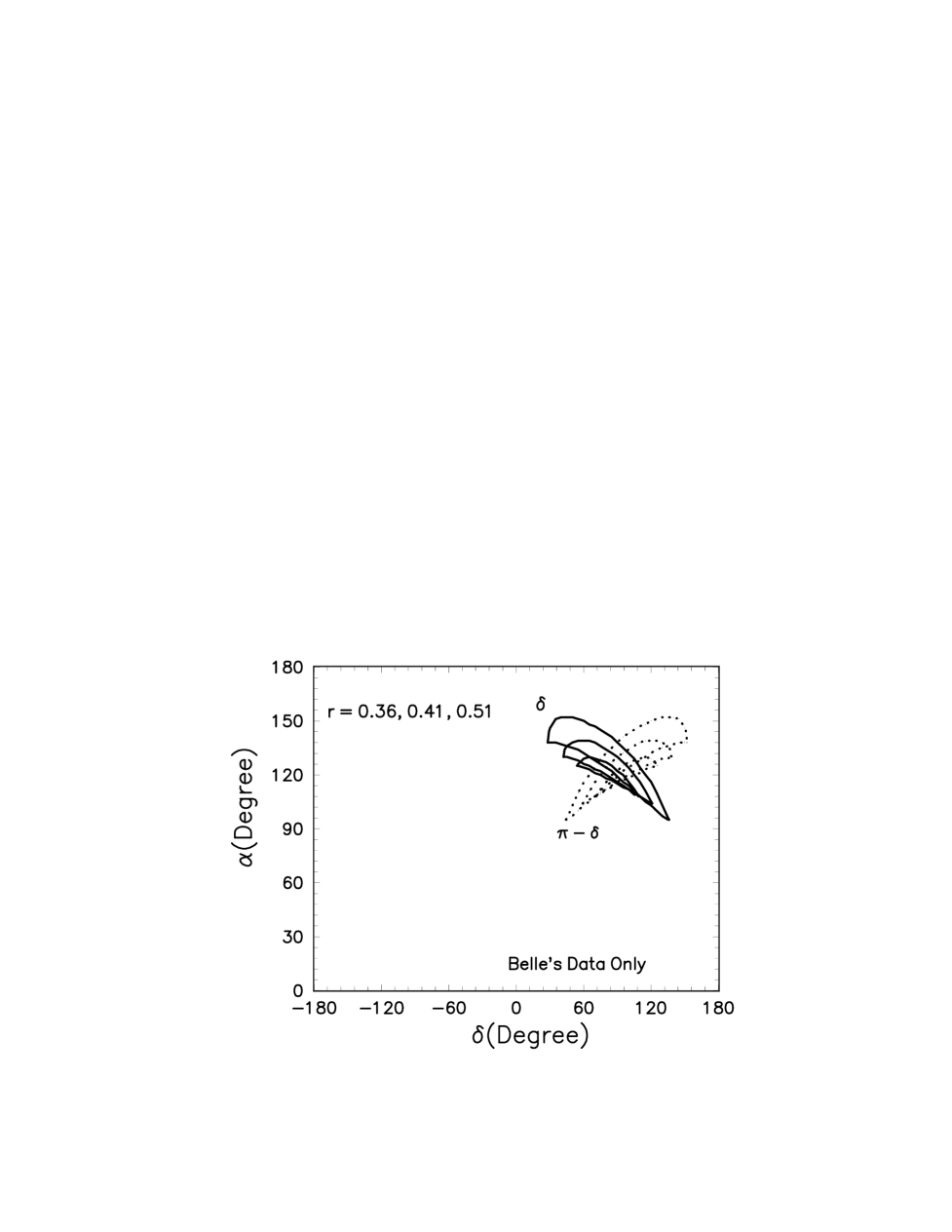
FIG. 6.: Contour plot of the asymmetries $S_{\pi\pi}$ and $A_{\pi\pi}$ versus the strong phase $\delta$ and CKM angle $\alpha$ for $r=0.36$ (small solid circle), $0.41$ (middle-sized solid circle ) and $0.51$ (large solid circle ), respectively. The dotted circles show the effects of discrete ambiguity. The regions inside each circle is still allowed by the Belle’s limits $S_{\pi\pi}^{exp}\leq-0.67$ and $A_{\pi\pi}^{exp}\geq 0.54$.

REFERENCES

- [1] BaBar Collaboration, B. Aubert et al., Phys. Rev. Lett. 87, 091801 (2001); BaBar Collaboration, J. Dorfan, BaBar results on CP violation, LP 2001, Roma, July 23-28, 2001; Babar-talk-01/77;
- [2] Babar Collaboration, B. Aubert et al., Improved measurement of CP violating asymmetry amplitude , hep-ex/0203007.
- [3] Belle Collaboration, K. Abe et al., Phys. Rev. Lett. 87, 091802 (2001); Belle Collaboration, S. L. Olsen, Measurement of , LP 2001, Roma, July 23-28, 2001; Belle LP-01;
- [4] Belle Collaboration, K. Abe et al., Observation of mixing-induced CP violation in the neutral B meson system, hep-ex/0202027;
- [5] Belle Collaboration, K. Abe et al., Study of CP violating asymmetry in decays, hep-ex/0204002.
- [6] BaBar Collaboration, B. Aubert et al., Measurements of branching fractions and CP violating asymmetries in decays, hep-ex/0207055, SLAC-PUB-9317.
- [7] BaBar Collaboration, B. Aubert et al., Phys. Rev. D 65, 051502(R) (2002).
- [8] BaBar Collaboration, B. Aubert et al., Measurements of branching fractions and CP violating asymmetries in decays, hep-ex/0205082.
- [9] M. Gronau and J. Rosner, Phys. Rev. D 65, 093012 (2002).
- [10] R. Fleischer, and J. Matias, hep-ph/0204101.
- [11] M. Kobayashi and T. Maskawa, Prog. Theor. Phys. 49, 652 (1973).
- [12] A.J. Buras, in Flavour Physics: CP violation and rare Decays, Lectures given at International School of Subnuclear Physics, Erice, Italy, 2000, hep-ph/0101336.
- [13] M. Gronau and D. London, Phys. Rev. Lett. 65, 3381 (1990).
- [14] A. Höcker, H. Lacker, S. Laplace and F.le Diberder, Eur. Phys. J. C 21, 225 (2001);
- [15] Particle Data group, D.E. Groom et al., Eur. Phys. J. C 15 1 (2000).
- [16] X.G. He, Y.K. Hsino, J.Q. Shi, Y.L. Wuand Y.F. Zhou, Phys. Rev. D 64, 034002 (2001).
- [17] A.F. Falk, Flavor physics and the CKM matrix: An overview, hep-ph/0201094.
- [18] Z.J. Xiao and M.P. Zhang, Phys. Rev. D 65, 114017 (2002).
- [19] D. Atwood and A. Soni, Phys. Lett. B 508, 17 (2001).
- [20] M. Beneke, G. Buchalla, M. Neubert and C.T. Sachrajda, Nucl. Phys. B 601, 245 (2001).
- [21] C.D. Lü, K. Ukai and M.Z. Yang, Phys. Rev. D 63, 074009 (2001).