NNLO ANALYSIS OF SEMILEPTONIC RARE $B$ DECAYS

We update the standard model predictions for the branching ratios of the decays $B\to(K,K^{*},X_{s})\;\ell^{+}\ell^{-}$, with $\ell=e,\;\mu$. Using the measurements of ${\cal B}(B\to X_{s}\gamma)$ and ${\cal B}(B\to K\ell^{+}\ell^{-})$ as well as the upper limits on ${\cal B}(B\to(K^{*},X_{s})\ell^{+}\ell^{-})$, we work out model independent bounds on the relevant Wilson coefficients. We show the impact of such bounds on the parameter space of the MSSM with minimal flavour violation and of supersymmetric models with additional sources of flavour changing.

1 Introduction

With increased statistical power of experiments at the $B$–factories, the exclusive and inclusive $B\to(K,K^{*},X_{s})\;\ell^{+}\ell^{-}$ decays will be measured very precisely, in the next several years. On the theoretical side, partial results in next-to-next-to-leading logarithmic accuracy are now available in the inclusive channels $B\to X_{s}\ell^{+}\ell^{-}$ $\!{}^{{\bf?},{\bf?}}$. In this talk, we review the status of the standard model predictions for the inclusive and exclusive modes and present the model independent constraints implied by the new data (see Ref. $\!{}^{{\bf?}}$ for a more detailed presentation of the results). The experimental input that we use in our analysis is given below. Except for the inclusive branching ratio for $B\to X_{s}\gamma$, which is the average of the results from CLEO $\!{}^{{\bf?}}$, ALEPH $\!{}^{{\bf?}}$ and BELLE $\!{}^{{\bf?}}$ measurements, all other entries are taken from the two BELLE papers listed in Ref. $\!{}^{{\bf?}}$:

$${\cal B}(B\to X_{s}\gamma) = (3.22\pm 0.40)\times 10^{-4}\;,$$ (1)

$${\cal B}(B\to K\mu^{+}\mu^{-}) = (0.99^{+0.40+0.13}_{-0.32-0.14})\times 10^{-6}\;,$$ (2)

$${\cal B}(B\to Ke^{+}e^{-}) = (0.48^{+0.32+0.09}_{-0.24-0.11})\times 10^{-6}\;,$$ (3)

$${\cal B}(B\to K\ell^{+}\ell^{-}) = (0.75^{+0.25}_{-0.21}\pm 0.09)\times 10^{-6}\;,$$ (4)

$${\cal B}(B\to K^{*}\mu^{+}\mu^{-}) \leq 3.0\times 10^{-6}\;{\rm at}\;{90\%\ \mathrm{C.L.}}\;,$$ (5)

$${\cal B}(B\to K^{*}e^{+}e^{-}) \leq 5.1\times 10^{-6}\;{\rm at}\;{90\%\ \mathrm{C.L.}}\;,$$ (6)

$${\cal B}(B\to X_{s}\mu^{+}\mu^{-}) \leq 19.1\times 10^{-6}\;{\rm at}\;{90\%\ \mathrm{C.L.}}\;,$$ (7)

$${\cal B}(B\to X_{s}e^{+}e^{-}) \leq 10.1\times 10^{-6}\;{\rm at}\;{90\%\ \mathrm{C.L.}}\;.$$ (8)

The upper bounds given in Eqs. (2) – (8) refer to the so–called non–resonant branching ratios integrated over the entire dilepton invariant mass spectrum. In the experimental analyses, judicious cuts are used to remove the dominant resonant contributions arising from the decays $B\to(X_{s},K,K^{*})(J/\psi,\psi^{\prime},...)\to(X_{s},K,K^{*})\ell^{+}\ell^{-}$. A direct comparison of experiment and theory is, of course, very desirable, but we do not have access to this restricted experimental information. Instead, we compare the theoretical predictions with data which has been corrected for the experimental acceptance using SM-based theoretical distributions. In the present analysis, we are assuming that the acceptance corrections have been adequately incorporated in the experimental analysis in providing the branching ratios and upper limits listed above. We will give the theoretical branching ratios integrated over all dilepton invariant masses to compare with these numbers. However, for future analyses, we emphasize the dilepton invariant mass distribution in the low-$\hat{s}$ region, $\hat{s}\equiv m_{\ell^{+}\ell^{-}}^{2}/m_{b,pole}^{2}\leq 0.25$, where the NNLO calculations for the inclusive decays are known, and resonant effects due to $J/\psi$, $\psi^{\prime}$, etc. are expected to be small.

The effective Hamiltonian in the SM inducing the $b\to s\ell^{+}\ell^{-}$ and $b\to s\gamma$ transitions is:

$${\cal H}_{\hbox{eff}}=-\frac{4G_{F}}{\sqrt{2}}V_{ts}^{*}V_{tb}\sum_{i=1}^{10}C_{i}(\mu)\,O_{i}(\mu)\quad,$$ (9)

where $O_{i}(\mu)$ are dimension-six operators at the scale $\mu$, $C_{i}(\mu)$ are the corresponding Wilson coefficients, $G_{F}$ is the Fermi coupling constant, and the CKM dependence has been made explicit. The operators can be chosen as in Ref. $\!{}^{{\bf?}}$

$$\begin{array}[]{rclrcl}O_{1}&=&(\bar{s}_{L}\gamma_{\mu}T^{a}c_{L})(\bar{c}_{L}\gamma^{\mu}T^{a}b_{L})\,,&O_{2}&=&(\bar{s}_{L}\gamma_{\mu}c_{L})(\bar{c}_{L}\gamma^{\mu}b_{L})\,,\\ \vspace{0.2cm}O_{3}&=&(\bar{s}_{L}\gamma_{\mu}b_{L})\sum_{q}(\bar{q}\gamma^{\mu}q)\,,&O_{4}&=&(\bar{s}_{L}\gamma_{\mu}T^{a}b_{L})\sum_{q}(\bar{q}\gamma^{\mu}T^{a}q)\,,\\ \vspace{0.2cm}O_{5}&=&(\bar{s}_{L}\gamma_{\mu_{1}}\gamma_{\mu_{2}}\gamma_{\mu_{3}}b_{L})\sum_{q}(\bar{q}\gamma^{\mu_{1}}\gamma^{\mu_{2}}\gamma^{\mu_{3}}q)\,,&O_{6}&=&(\bar{s}_{L}\gamma_{\mu_{1}}\gamma_{\mu_{2}}\gamma_{\mu_{3}}T^{a}b_{L})\sum_{q}(\bar{q}\gamma^{\mu_{1}}\gamma^{\mu_{2}}\gamma^{\mu_{3}}T^{a}q)\,,\vspace{0.2cm}\\ \vspace{0.2cm}O_{7}&=&\frac{e}{g_{s}^{2}}m_{b}(\bar{s}_{L}\sigma^{\mu\nu}b_{R})F_{\mu\nu}\,,&O_{8}&=&\frac{1}{g_{s}}m_{b}(\bar{s}_{L}\sigma^{\mu\nu}T^{a}b_{R})G_{\mu\nu}^{a}\,,\\ \vspace{0.2cm}O_{9}&=&\frac{e^{2}}{g_{s}^{2}}(\bar{s}_{L}\gamma_{\mu}b_{L})\sum_{\ell}(\bar{\ell}\gamma^{\mu}\ell)\,,&O_{10}&=&\frac{e^{2}}{g_{s}^{2}}(\bar{s}_{L}\gamma_{\mu}b_{L})\sum_{\ell}(\bar{\ell}\gamma^{\mu}\gamma_{5}\ell)\,,\end{array}$$

where the subscripts $L$ and $R$ refer to left- and right- handed components of the fermion fields.

2 Expectations in the standard model

Table 1: SM predictions at NNLO accuracy for the various inclusive and exclusive decays involving the quark transition $b\to s\ell^{+}\ell^{-}$. For the exclusive channels the indicated errors correspond to variations of the form factors, $\mu_{b}$, $m_{t,pole}$ and $m_{c}/m_{b}$, respectively. For the inclusive channels the errors correspond, respectively, to variations of $\mu_{b}$, $m_{t,pole}$ and $m_{c}/m_{b}$. In the last column we add the errors in quadrature.                                                     

$B\to K\ell^{+}\ell^{-}$	$\left(0.35\pm 0.11\pm 0.04\pm 0.02\pm 0.0005\right)\times 10^{-6}$	$\left(0.35\pm 0.12\right)\times 10^{-6}$ [
$B\to K^{*}e^{+}e^{-}$	$\left(1.58\pm 0.47\pm 0.12^{+0.06}_{-0.08}\pm 0.04\right)\times 10^{-6}$	$\left(1.58\pm 0.49\right)\times 10^{-6}$ [
$B\to K^{*}\mu^{+}\mu^{-}$	$\left(1.19\pm 0.36\pm 0.12^{+0.06}_{-0.08}\pm 0.04\right)\times 10^{-6}$	$\left(1.19\pm 0.39\right)\times 10^{-6}$ [
$B\to X_{s}\mu^{+}\mu^{-}$	$\left(4.15\pm 0.27\pm 0.21\pm 0.62\right)\times 10^{-6}$	$\left(4.15\pm 0.70\right)\times 10^{-6}$ [
$B\to X_{s}e^{+}e^{-}$	$\left(6.89\pm 0.37\pm 0.25\pm 0.91\right)\times 10^{-6}$	$\left(6.89\pm 1.01\right)\times 10^{-6}$ [

The SM predictions for semileptonic rare $B$ decays are summarized in table 1.

Note that a genuine NNLO calculation of the inclusive branching ratios only exists for values of $\hat{s}$ below 0.25. For high values of $\hat{s}$, an estimate of the NNLO result is obtained by an extrapolation procedure. It is possible to show $\!{}^{{\bf?}}$, that the full NNLO invariant mass distribution is very well approximated, in the entire low-$\hat{s}$ range, by the partial NNLO for the choice of the scale $\mu=2.5\;{\hbox{GeV}}$. This is yet another illustration of the situation often met in perturbation theory that a judicious choice of the scale reduces the higher order corrections. It seems, therefore, reasonable to use the partial NNLO curve corresponding to $\mu_{b}=2.5\;{\hbox{GeV}}$ as an estimate for the central value of the full NNLO for $\hat{s}>0.25$.

For what concerns the exclusive decays $B\to K^{(*)}\ell^{+}\ell^{-}$, we implement the NNLO corrections calculated by Bobeth et al. $\!{}^{{\bf?}}$ and by Asatrian et al. $\!{}^{{\bf?}}$ for the short-distance contribution. Then, we use the form factors calculated with the help of the QCD sum rules in Ref. $\!{}^{{\bf?}}$. In order to accommodate present data on the $B\to K^{*}\gamma$ decay, we use the minimum allowed form factors, given in Table 5 of Ref. $\!{}^{{\bf?}}$, as our default set. In our numerical analysis, we add a flat $\pm 15\%$ error as residual uncertainty on the form factors.

Let us stress once more that, from a theoretical point of view, would be much better to compare the non–resonant branching ratios integrated in the low–$\hat{s}$ region with the corresponding experimental bounds. Defining such region according to the Belle analysis presented in Ref. $\!{}^{{\bf?}}$, we choose the integration limits as follows:

$$B\to X_{s}e^{+}e^{-}:\;\left(0.2\;{\hbox{GeV}}\over m_{b}\right)^{2}\leq\hat{s}\leq\left(M_{J/\Psi}-0.6\;{\hbox{GeV}}\over m_{b}\right)^{2}\,,$$ (10)

$$B\to X_{s}\mu^{+}\mu^{-}:\;\left(2m_{\mu}\over m_{b}\right)^{2}\leq\hat{s}\leq\left(M_{J/\Psi}-0.35\;{\hbox{GeV}}\over m_{b}\right)^{2}\;.$$ (11)

For the integrated branching ratios in the SM we find:

$${\cal B}(B\to X_{s}e^{+}e^{-})\Big{|}_{\rm low} = \left(2.47\pm 0.40\right)\times 10^{-6}\;\;\;(\delta{\cal B}_{X_{s}ee}=\pm 16\%)\;,$$ (12)

$${\cal B}(B\to X_{s}\mu^{+}\mu^{-})\Big{|}_{\rm low} = \left(2.75\pm 0.45\right)\times 10^{-6}\;\;\;(\delta{\cal B}_{X_{s}\mu\mu}=\pm 16\%)\;.$$ (13)

3 Model independent analysis

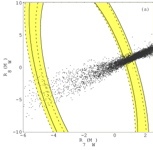
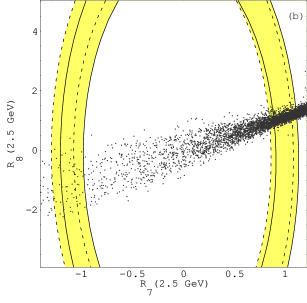
Figure 1: ${90\%\ \mathrm{C.L.}}$ bounds in the $[R_{7}(\mu),R_{8}(\mu)]$ plane following from the world average $B\to X_{s}\gamma$ branching ratio for $\mu=m_{W}$ (left-hand plot) and $\mu=2.5$ GeV (right-hand plot). Theoretical uncertainties are taken into account. The solid and dashed lines correspond to the $m_{c}=m_{c,pole}$ and $m_{c}=m_{c}^{\overline{MS}}(\mu_{b})$ cases respectively. The scatter points correspond to the expectation in MFV models (the ranges of the SUSY parameters are specified in the text).

In our analysis, we make the assumption that the dominant new physics effects can be implemented by using the SM operator basis for the effective hamiltonian. The Wilson coefficients that are constrained by the set of measurements given in Eqs. (1)–(8) are $C_{7,8,9,10}$. Note that $b\to s\ell^{+}\ell^{-}$ transitions depend on $C_{7}$ and $C_{8}$ only through the effective coefficient $A_{7}(C_{7},C_{8})$ $\!{}^{{\bf?}}$. Our first step consists in writing ${\cal B}(B\to X_{s}\gamma)$ as a function of $R_{7,8}(\mu)\equiv A_{7,8}^{\rm tot}(\mu)/A_{7,8}^{\rm SM}(\mu)$ (following Ref. $\!{}^{{\bf?}}$) and plotting the regions in the $[R_{7},R_{8}]$ plane that are allowed by Eq. (1). Requiring $|R_{8}(\mu_{W})|\leq 10$ in order to satisfy the constraints from the decays $B\to X_{s}g$ and $B\to X_{c\!\!/}$ (where $X_{c\!\!/}$ denotes any hadronic charmless final state) we are, then, able to extract the bounds on $A_{7}(\mu_{b})$. It was recently pointed out in Ref. $\!{}^{{\bf?}}$ that the charm mass dependence of the $B\to X_{s}\gamma$ branching ratio was underestimate in all the previous analyses. Indeed, the replacement of the pole mass ($m_{c,pole}/m_{b,pole}=0.29\pm 0.02$) with the $\overline{MS}$ running mass ($m_{c}^{\overline{MS}}(\mu_{b})/m_{b,pole}=0.22\pm 0.04$) increases the branching ratio of about $11\%$. In order to take into account this additional source of uncertainty, we work out the constraints on the Wilson coefficients for both choices of the charm mass; we will then use the loosest bounds in the $b\to s\ell^{+}\ell^{-}$ analysis. We present the resulting allowed regions in Figs. 1a and 1b (note that according to the previous discussion we are interested in the bounds at $\mu_{b}=2.5\;{\hbox{GeV}}$). The regions in Fig. 1b translate in the following allowed constraints:

$$\cases{m_{c}/m_{b}=0.29:\;\;\;A_{7}^{\rm tot}(2.5\;{\hbox{GeV}})\in[-0.37,-0.18]\;\&\;[0.21,0.40]\;,&\cr m_{c}/m_{b}=0.22:\;\;\;A_{7}^{\rm tot}(2.5\;{\hbox{GeV}})\in[-0.35,-0.17]\;\&\;[0.25,0.43]\;.&\cr}$$ (14)

In the subsequent numerical analysis we impose the union of the above allowed ranges

$$-0.37\leq A_{7}^{\rm tot,<0}(2.5\;{\hbox{GeV}})\leq-0.17 \& 0.21\leq A_{7}^{\rm tot,>0}(2.5\;{\hbox{GeV}})\leq 0.43$$ (15)

calling them $A_{7}^{\rm tot}$–positive and $A_{7}^{\rm tot}$–negative solutions.

The bounds in the $[C_{9}^{NP}(\mu_{W}),C_{10}^{NP}]$ plane, implied by the experimental results (2)–(8) are summarized in Fig. 2, where the two plots correspond respectively to the $A_{7}^{\rm tot}$–positive and $A_{7}^{\rm tot}$–negative solutions just discussed. Note that the overall allowed region is driven by the constraints emanating from the decays $B\to X_{s}e^{+}e^{-}$ (outer contours) and $B\to K\mu^{+}\mu^{-}$ (inner contours).

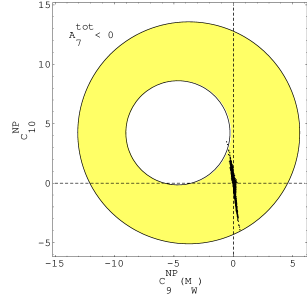
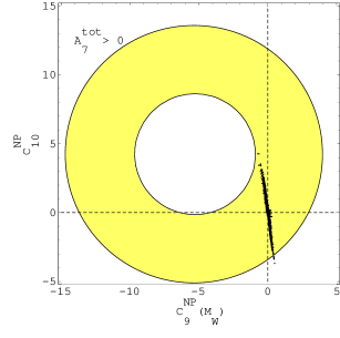
Figure 2: NNLO Case. Superposition of all the constraints. The plots correspond to the $A_{7}^{\rm tot}(2.5\;{\hbox{GeV}})<0$ and $A_{7}^{\rm tot}(2.5\;{\hbox{GeV}})>0$ case, respectively. The points are obtained by means of a scanning over the EMFV parameter space and requiring the experimental bound from $B\to X_{s}\gamma$ to be satisfied.                                                

4 Expectation in supersymmetry

In this section we analyze the impact of the $b\to s\gamma$ and $b\to s\ell^{+}\ell^{-}$ experimental constraints on several supersymmetric models. We will first discuss the more restricted framework of the minimal flavour violating MSSM, and then extend the analysis to more general models in which new SUSY flavour changing couplings are allowed.

4.1 Minimal flavour violation

As already known from the existing literature (see for instance Ref. $\!{}^{{\bf?}}$), minimal flavour violating (MFV) contributions are generally too small to produce sizable effects on the Wilson coefficients $C_{9}$ and $C_{10}$. In the MFV scheme all the genuine new sources of flavour changing transitions other than the CKM matrix are switched off, and the low energy theory depends only on the following parameters: $\mu$, $M_{2}$, $\tan\beta$, $M_{H^{\pm}}$, $M_{\tilde{t}_{2}}$ and $\theta_{\tilde{t}}$ (see Ref. $\!{}^{{\bf?}}$ for a precise definition of the various quantities). Scanning over this parameter space and taking into account the lower bounds on the sparticle masses as well as the $b\to s\gamma$ constraint given in Eq. (1), we derive the ranges for the new physics contributions to $C_{9}$ and $C_{10}$. In order to produce bounds that can be compared with the model independent allowed regions plotted in Fig. 2, we divided the surviving SUSY points in two sets, according to the sign of $A_{7}^{\rm tot}$:

$$A_{7}^{\rm tot}<0\Rightarrow\cases{C_{9}^{MFV}(\mu_{W})\in[-0.2,0.4]\,,\cr C_{10}^{MFV}\in[-1.0,0.7]}\,.$$ (16)

$$A_{7}^{\rm tot}>0\Rightarrow\cases{C_{9}^{MFV}(\mu_{W})\in[-0.2,0.3]\,,\cr C_{10}^{MFV}\in[-0.8,0.5]\;.}$$ (17)

We stress that the above discussion applies to any supersymmetric model with flavour universal soft-breaking terms, such as minimal supergravity MSSM and gauge-mediated supersymmetry breaking models. Beyond-the-SM flavour violations in such models are induced only via renormalization group running, and are tiny. Hence, they can be described by MFV models discussed in this paper.

Before finishing this subsection and starting our discussion on models with new flavour changing interactions, let us show in more detail the impact of $b\to s\gamma$ on MFV models. The scatter plot presented in Fig. 1 is obtained varying the various MFV SUSY parameters and shows the strong correlation between the values of the Wilson coefficients $C_{7}$ and $C_{8}$. In fact, the SUSY contributions to the magnetic and chromo–magnetic coefficients differ only because of colour factors and loop-functions.

4.2 Chargino contributions: Extended–MFV models

A basically different scenario arises if chargino–mediated penguin and box diagrams are considered in connection with non–vanishing mass insertions (See Ref. $\!{}^{{\bf?}}$ for a definition of the so–called mass insertion approximation (MIA)). As can be inferred by Table 4 in Ref. $\!{}^{{\bf?}}$, the presence of a light $\tilde{t}_{2}$ generally gives rise to large contributions to $C_{9}$ and especially to $C_{10}$. In the following, we will concentrate on the so–called Extended MFV (EMFV) models introduced in Ref. $\!{}^{{\bf?}}$. In these models we can fully exploit the impact of chargino penguins with a light $\tilde{t}$ still working with a limited number of free parameters. EMFV models are based on the heavy squarks and gluino assumption. In this framework, the charged Higgs and the lightest chargino and stop masses are allowed to be light while the rest of the SUSY spectrum is assumed to be degenerate and heavier than $1\;{\hbox{TeV}}$. The assumption of a heavy gluino suppresses any possible gluino–mediated SUSY contribution to low energy observables. Note that even in the presence of a light gluino these penguin diagrams remain suppressed due to the heavy down squarks present in the loop. In the MIA approach, a diagram can contribute sizably only if the inserted mass insertions involve the light stop. This leaves us with only two unsuppressed flavour changing sources other than the CKM matrix, namely the mixings $\tilde{u}_{L}-\tilde{t}_{2}$ (denoted by $\delta_{\tilde{u}_{L}\tilde{t}_{2}}$) and $\tilde{c}_{L}-\tilde{t}_{2}$ (denoted by $\delta_{\tilde{c}_{L}\tilde{t}_{2}}$). The phenomenological impact of $\delta_{\tilde{t}_{2}\tilde{u}_{L}}$ has been studied in Ref. $\!{}^{{\bf?}}$ and its impact on the $b\to s\gamma$ and $b\to s\ell^{+}\ell^{-}$ transitions is indeed negligible. Therefore, we are left with the MIA parameter $\delta_{\tilde{t}_{2}\tilde{c}_{L}}$ only. Scanning over the SUSY parameter space ($\mu$, $M_{2}$, $\tan\beta$, $M_{\tilde{t}_{2}}$, $\sin\theta_{\tilde{t}}$, $M_{H^{\pm}}$, $M_{\tilde{\nu}}$ and $\delta_{\tilde{t}_{2}\tilde{c}_{L}}$) and imposing the constraints from the sparticle masses lower bounds and $B\to X_{s}\gamma$, we obtain the points plotted in Fig. 2. Note that these SUSY models can account only for a small part of the region allowed by the model independent analysis of current data.

5 Conclusions

We have presented theoretical branching ratios, model independent analyses and SUSY predictions for the rare $B$ decays $B\to X_{s}\ell^{+}\ell^{-}$ and $B\to(K,K^{*})\ell^{+}\ell^{-}$, incorporating the NNLO improvements. The dilepton invariant mass spectrum is calculated in the NNLO precision in the low dilepton invariant mass region, $\hat{s}<0.25$ and an extrapolation is used for $\hat{s}>0.25$. Current B factory experiments will soon probe these decays at the level of the SM sensitivity and we stress the need to measure the inclusive decays $B\to X_{s}\ell^{+}\ell^{-}$ in the low dilepton mass range for a proper comparison with the SM expectations.

References

References

- [1] C. Bobeth, M. Misiak and J. Urban, Nucl. Phys. B 574 (2000) 291.
- [2] H. H. Asatrian, H. M. Asatrian, C. Greub and M. Walker, Phys. Lett. B 507 (2001) 162; Phys. Rev. D 65 (2002) 074004; hep-ph/0204341.
- [3] A. Ali, C. Greub, G. Hiller, E. Lunghi, hep-ph/0112300.
- [4] S. Chen et al. [CLEO Collaboration], Phys. Rev. Lett. 87 (2001) 251807.
- [5] R. Barate et al. [ALEPH Collaboration], Phys. Lett. B 429 (1998) 169.
- [6] K. Abe et al. [BELLE Collaboration], Phys. Lett. B 511 (2001) 151.
-
[7]
K. Abe et al. [BELLE Collaboration], BELLE-CONF-0110 [hep-ex/0107072];
K. Abe et al. [BELLE Collaboration], Phys. Rev. Lett. 88 (2002) 021801. - [8] A. Ali, P. Ball, L. T. Handoko and G. Hiller, Phys. Rev. D 61 (2000) 074024.
- [9] A. L. Kagan and M. Neubert, Eur. Phys. J. C 7 (1999) 5.
- [10] P. Gambino and M. Misiak, Nucl. Phys. B 611 (2001) 338.
- [11] E. Lunghi, A. Masiero, I. Scimemi and L. Silvestrini, Nucl. Phys. B 568 (2000) 120.
-
[12]
L. J. Hall, V. A. Kostelecky, and S. Raby, Nucl. Phys. B 267 (1986) 415;
A. J. Buras, A. Romanino, and L. Silvestrini, Nucl. Phys. B 520 (1998) 3. - [13] A. Ali and E. Lunghi, Eur. Phys. J. C 21 (2001) 683.