July, 2002

Nonresonant Three-body Decays of $D$ and $B$ Mesons

Hai-Yang Cheng^1,2 and Kwei-Chou Yang³

¹ Institute of Physics, Academia Sinica

Taipei, Taiwan 115, Republic of China

² C.N. Yang Institute for Theoretical Physics, State University of New York

Stony Brook, New York 11794

³ Department of Physics, Chung Yuan Christian University

Chung-Li, Taiwan 320, Republic of China

Abstract

Nonresonant three-body decays of $D$ and $B$ mesons are studied. It is pointed out that if heavy meson chiral perturbation theory (HMChPT) is applied to the heavy-light strong and weak vertices and assumed to be valid over the whole kinematic region, then the predicted decay rates for nonresonant charmless 3-body $B$ decays will be too large and especially $B^{-}\to\pi^{-}K^{+}K^{-}$ greatly exceeds the current experimental limit. This can be understood as chiral symmetry has been applied there twice beyond its region of validity. If HMChPT is applied only to the strong vertex and the weak transition is accounted for by the form factors, the dominant $B^{*}$ pole contribution to the tree-dominated direct three-body $B$ decays will become small and the branching ratio will be of order $10^{-6}$. The decay modes $B^{-}\to(K^{-}h^{+}h^{-})_{\rm NR}$ and $\overline{B}^{0}\to(\overline{K}^{0}h^{+}h^{-})_{\rm NR}$ for $h=\pi,K$ are penguin dominated. We apply HMChPT in two different cases to study the direct 3-body $D$ decays and compare the results with experiment. The preliminary FOCUS measurement of the direct decay $D_{s}^{+}\to(\pi^{+}\pi^{+}\pi^{-})_{\rm NR}$ may provide the first indication of the importance of final-state interactions for the weak annihilation process in nonresonant $D$ decays. Theoretical uncertainties are discussed.

I Introduction

The three-body decays of heavy mesons are in general dominated by intermediate (vector or scalar) resonances, namely, they proceed via quasi-two-body decays containing a resonance state and a pseudoscalar meson. The analysis of these decays using the Dalitz plot technique enables one to study the properties of various resonances. The nonresonant contribution is usually a small fraction of the total 3-body decay rate. Nevertheless, its study is important for several reasons. First, the interference between resonant and nonresonant decay amplitudes in $B$ decays may provide information on the CP-violating phase angles [2, 3, 4, 5, 6, 7]. For example, the interference between $B^{-}\to(\pi^{+}\pi^{-}\pi^{-})_{\rm NR}$ and $B^{-}\to\chi_{c0}\pi^{-}$ could lead to a measurable $CP$ asymmetry characterized by the phase angle $\gamma$ [2], while the Dalitz plot analysis of $B\to\rho\pi\to\pi\pi\pi$ allows one to measure the angle $\alpha$. Second, an inadequate extraction of the nonresonant contribution could yield incorrect measurements for the resonant channels [8]. Third, some of nonresonant 3-body $D$ decays have been measured. It is thus important to understand their underlying mechanisms. Experimentally, it is hard to measure the direct 3-body decays as the interference between nonresonant and quasi-two-body amplitudes makes it difficult to disentangle these two distinct contributions and extract the nonresonant one.

The direct three-body decays of mesons in general receive two distinct contributions: one from the point-like weak transition and the other from the pole diagrams which involve four-point strong vertices. For $D$ decays, attempts of applying the effective $SU(4)\times SU(4)$ chiral Lagrangian to describe the $DP\to DP$ and $PP\to PP$ scattering at energies $\sim m_{D}$ have been made by several authors [9, 10, 11, 12, 13] to calculate the nonresonant $D$ decays, though in principle it is not justify to employ the SU(4) chiral symmetry. As shown in [12, 13], the predictions of the nonresonant decay rates in chiral perturbation theory are in general too small when compared with experiment.

With the advent of heavy quark symmetry and its combination with chiral symmetry [14, 15, 16], the nonresonant $D$ decays can be studied reliably at least in the kinematical region where the final pseuodscalar mesons are soft. Some of the direct 3-body $D$ decays were studied based on this approach [17, 18].

Nonresonant charmless three-body $B$ decays have been recently studied extensively based on heavy meson chiral perturbation theory (HMChPT). However, the predicted decay rates are unexpectedly large. For example, the branching ratio of $B^{-}\to(\pi^{+}\pi^{-}\pi^{-})_{\rm NR}$ is predicted to be of order $10^{-5}$ in [2] and [3]. Therefore, it has a decay rate larger than the two-body counterpart $B\to\pi\pi$. However, it is found in [6] that the dominant $B^{*}$ pole contribution to the nonresonant $B^{-}\to\pi^{+}\pi^{-}\pi^{-}$ accounts for a branching ratio of order only $1\times 10^{-6}$. Recently, Belle [19] and BaBar [20] have measured several charmless three-body $B$ decays without making any assumptions on the intermediate resonance states [19]. The predicted branching ratio of order $3\times 10^{-5}$ in [3] for $B^{-}\to(K^{-}K^{+}\pi^{-})_{\rm NR}$ already exceeds the upper limit $1.2\times 10^{-5}$ by Belle [19] and $7\times 10^{-6}$ by BaBar [20] for resonant and nonresonant contributions. Likewise, the predicted ${\cal B}(B^{-}\to\pi^{+}\pi^{-}\pi^{-})_{\rm NR}\approx 4\times 10^{-5}$ in [3] is too large compared to the limit $1.5\times 10^{-5}$ set by BaBar. Therefore, it is important to reexamine and clarify the existing calculations.

The issue has to do with the applicability of HMChPT. In order to apply this approach, two of the final-state pseudoscalars have to be soft. The momentum of the soft pseudoscalar should be smaller than the chiral symmetry breaking scale $\Lambda_{\chi}\sim 830$ MeV. For 3-body charmless $B$ decays, the available phase space where chiral perturbation theory is applicable is only a small fraction of the whole Dalitz plot. Therefore, it is not justified to apply chiral and heavy quark symmetries to a certain kinematic region and then generalize it to the region beyond its validity. In order to have a reliable prediction for the total rate of direct 3-body decays, one should try to utilize chiral symmetry to a minimum. Therefore, we will apply HMChPT only to the strong vertex and use the form factors to describe the weak vertex. In contrast, for direct 3-body $D$ decays, the allowed phase space region where HMChPT is applicable can be a dominant one for some decay modes.

The paper is organized as follows. After introducing the effective Hamiltonian in Sec. II we proceed to discuss the difficulties with HMChPT when applying it to describe the 3-body nonresonant $B$ decays in the whole Dalitz plot and its possible remedy. The full amplitude for the penguin-dominated $B^{-}\to K^{-}\pi^{+}\pi^{-}$ is worked out as an example. The direct 3-body $D$ decays are discussed in Sec. III. Discussions of theoretical uncertainties and conclusions are presented in Sec. IV.

II Nonresonant three-body decays of $B$ mesons

A Hamiltonian

The relevant effective $\Delta B=1$ weak Hamiltonian for charmless hadronic $B$ decays is

$${\cal H}_{\rm eff}(\Delta B=1) = {G_{F}\over\sqrt{2}}\Bigg{\{}V_{ub}V_{uq}^{*}\Big{[}c_{1}(\mu)O_{1}^{u}(\mu)+c_{2}(\mu)O_{2}^{u}(\mu)\Big{]}+V_{cb}V_{cq}^{*}\Big{[}c_{1}(\mu)O_{1}^{c}(\mu)+c_{2}(\mu)O_{2}^{c}(\mu)\Big{]}$$ (2)

$$-V_{tb}V_{tq}^{*}\sum^{10}_{i=3}c_{i}(\mu)O_{i}(\mu)\Bigg{\}}+{\rm h.c.},$$

where $q=d,s$, and

$$O_{1}^{u}=(\bar{u}b)_{{}_{V-A}}(\bar{q}u)_{{}_{V-A}},\qquad\qquad\qquad\qquad~{}~{}O_{2}^{u}=(\bar{u}_{\alpha}b_{\beta})_{{}_{V-A}}(\bar{q}_{\beta}u_{\alpha})_{{}_{V-A}},$$ (3)

$$O_{1}^{c}=(\bar{c}b)_{{}_{V-A}}(\bar{q}c)_{{}_{V-A}},\qquad\qquad\qquad\qquad~{}~{}~{}O_{2}^{c}=(\bar{c}_{\alpha}b_{\beta})_{{}_{V-A}}(\bar{q}_{\beta}c_{\alpha})_{{}_{V-A}},$$ (4)

$$O_{3(5)}=(\bar{q}b)_{{}_{V-A}}\sum_{q^{\prime}}(\bar{q}^{\prime}q^{\prime})_{{{}_{V-A}}({{}_{V+A}})},\qquad\qquad O_{4(6)}=(\bar{q}_{\alpha}b_{\beta})_{{}_{V-A}}\sum_{q^{\prime}}(\bar{q}^{\prime}_{\beta}q^{\prime}_{\alpha})_{{{}_{V-A}}({{}_{V+A}})},$$ (5)

$$O_{7(9)}={3\over 2}(\bar{q}b)_{{}_{V-A}}\sum_{q^{\prime}}e_{q^{\prime}}(\bar{q}^{\prime}q^{\prime})_{{{}_{V+A}}({{}_{V-A}})},\qquad O_{8(10)}={3\over 2}(\bar{q}_{\alpha}b_{\beta})_{{}_{V-A}}\sum_{q^{\prime}}e_{q^{\prime}}(\bar{q}^{\prime}_{\beta}q^{\prime}_{\alpha})_{{{}_{V+A}}({{}_{V-A}})},$$ (6)

with $O_{3}$–$O_{6}$ being the QCD penguin operators, $O_{7}$–$O_{10}$ the electroweak penguin operators and $(\bar{q}_{1}q_{2})_{{}_{V\pm A}}\equiv\bar{q}_{1}\gamma_{\mu}(1\pm\gamma_{5})q_{2}$. The scale dependent Wilson coefficients calculated at next-to-leading order are renormalization scheme dependent. In the factorization approach the decay amplitude has the form

$$A(B\to M_{1}M_{2}M_{3})\propto\sum a_{i}\langle M_{1}M_{2}M_{3}|O_{i}|B\rangle,$$ (7)

where the coefficients $a_{i}$ are renormalization scale and $\gamma_{5}$-scheme independent. In ensuing calculations we will employ the values of $a_{i}$ listed in [21]. For $D$ decays we will use

$$a_{1}=1.20\,,\qquad\qquad a_{2}=-0.67\,.$$ (8)

B Difficulties with heavy meson chiral perturbation theory for nonresonant $B$ decays

The nonresonant three-body $B$ decays have been studied in two distinct methods, though both are based on heavy quark symmetry. One relies heavily on chiral perturbation theory to evaluate the 3-body matrix elements [3, 4, 22], whereas the use of chiral symmetry is restricted to the strong vertex for the other case [2, 6]. The resulting decay rates can be different by one to two orders of magnitude.

Let us first recapitulate the approach of heavy meson chiral perturbation theory [14, 15, 16] and consider the decay mode $B^{-}\to(K^{-}K^{+}\pi^{-})_{\rm NR}$ as an illustration. Since this decay is tree dominated, we will focus on the dominant contribution from the four-quark operator $O_{1}$

$$A(B^{-}\to K^{-}(p_{1})K^{+}(p_{2})\pi^{-}(p_{3}))={G_{F}\over\sqrt{2}}V_{ub}V_{ud}^{*}\,a_{1}\langle K^{-}K^{+}\pi^{-}|O_{1}|B^{-}\rangle.$$ (9)

Under the factorization approximation,

$$\langle K^{-}K^{+}\pi^{-}|O_{1}|B^{-}\rangle = \langle\pi^{-}|(\bar{d}u)_{{}_{V-A}}|0\rangle\langle K^{-}K^{+}|(\bar{u}b)_{{}_{V-A}}|B^{-}\rangle$$ (10)

$$+ \langle K^{-}K^{+}\pi^{-}|(\bar{d}u)_{{}_{V-A}}|0\rangle\langle 0|(\bar{u}b)_{{}_{V-A}}|B^{-}\rangle.$$ (11)

The second term on the right hand side corresponds to weak annihilation and it is expected to be helicity suppressed. As we shall see below, it indeed vanishes in the chiral limit.

The three-body matrix element $\langle K^{-}K^{+}|(\bar{u}b)_{{}_{V-A}}|B^{-}\rangle$ has the general expression [23]

$$\langle K^{-}(p_{1})K^{+}(p_{2})|(\bar{u}b)_{{}_{V-A}}|B^{-}(p_{B})\rangle = ir(p_{B}-p_{1}-p_{2})_{\mu}+i\omega_{+}(p_{2}+p_{1})_{\mu}$$ (12)

$$+ i\omega_{-}(p_{2}-p_{1})_{\mu}+h\epsilon_{\mu\nu\alpha\beta}p_{B}^{\nu}(p_{2}+p_{1})^{\alpha}(p_{2}-p_{1})^{\beta},$$ (13)

where $r$, $\omega_{\pm}$ and $h$ are the unknown form factors. When pseudoscalar mesons are soft, the heavy-to-light current in the heavy quark limit can be expressed in terms of a heavy meson and light pseudoscalar mesons [15, 14]. The weak current $L^{\mu}_{a}=\bar{q}_{a}\gamma_{\mu}(1-\gamma_{5})Q$, when written in terms of a heavy meson and light pseudoscalars, has the form [15]

$$L^{\mu}_{a}={if_{H_{b}}\sqrt{m_{H_{b}}}\over 2}\,{\rm Tr}[\gamma^{\mu}(1-\gamma_{5})H_{b}\xi_{ba}^{\dagger}]$$ (14)

to the lowest order in the light meson derivatives, where $H_{a}$ contains the pseudoscalar meson $P_{a}$ and the vector-meson field $P^{*}_{a\mu}$:

$$H_{a}=\sqrt{m_{H_{a}}}\,{1+v\!\!\!/\over 2}(P_{a\mu}^{*}\gamma^{\mu}-P_{a}\gamma_{5}),$$ (15)

where $v$ is the velocity of the heavy meson and $\xi^{2}$ is equal to the unitary matrix $U$ which describes the Goldstone bosons. The general expression of the matrix $U$ up to the fourth order in the meson matrix $\phi$ is [24]

$$U=1+2i{\phi\over f_{\pi}}-2{\phi^{2}\over f_{\pi}^{2}}-ia_{3}{\phi^{3}\over f_{\pi}^{3}}+2(a_{3}-1){\phi^{4}\over f_{\pi}^{4}}+\cdots,$$ (16)

where $a_{3}$ indicates the nonlinear chiral realization and it has the well-known value ${4\over 3}$ in the usual exponential expression for $U$, namely, $U={\rm exp}(i2\phi/f_{\pi})$. Here we do not specify the value of $a_{3}$ in order to demonstrate that the physical quantity is independent of the choice of chiral realization, i.e. the value of $a_{3}$. The traceless meson matrix $\phi$ reads

$$\phi=\left(\matrix{{\pi^{0}\over\sqrt{2}}+{\eta\over\sqrt{6}}&\pi^{+}&K^{+}\cr\pi^{-}&-{\pi^{0}\over\sqrt{2}}+{\eta\over\sqrt{6}}&K^{0}\cr K^{-}&\overline{K}^{0}&-\sqrt{2\over 3}\,\eta\cr}\right).$$ (17)

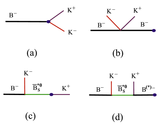
FIG. 1.: Point-like and pole diagrams responsible for the $B^{-}\to K^{-}K^{+}$ matrix element of the current $\bar{u}\gamma_{\mu}(1-\gamma_{5})b$, where the symbol $\bullet$ denotes an insertion of the current.

To compute the form factors $r$, $\omega_{\pm}$ and $h$, one needs to consider not only the point-like contact diagram, Fig. 1(a), but also various pole diagrams shown in Fig. 1. The heavy meson chiral Lagrangian given in [14, 15, 16] is needed to compute the strong $B^{*}BP$, $B^{*}B^{*}P$ and $BBPP$ vertices. The results for the form factors are [23, 3]

$$\omega_{+} = -{g\over f_{\pi}^{2}}\,{f_{B_{s}^{*}}m_{B_{s}^{*}}\sqrt{m_{B}m_{B_{s}^{*}}}\over t-m_{B_{s}^{*}}^{2}}\left[1-{(p_{B}-p_{1})\cdot p_{1}\over m_{B_{s}^{*}}^{2}}\right]+{f_{B}\over 2f_{\pi}^{2}},$$ (18)

$$\omega_{-} = {g\over f_{\pi}^{2}}\,{f_{B_{s}^{*}}m_{B_{s}^{*}}\sqrt{m_{B}m_{B_{s}^{*}}}\over t-m_{B_{s}^{*}}^{2}}\left[1+{(p_{B}-p_{1})\cdot p_{1}\over m_{B_{s}^{*}}^{2}}\right],$$ (19)

$$r = {f_{B}\over 2f_{\pi}^{2}}-{f_{B}\over f_{\pi}^{2}}\,{p_{B}\cdot(p_{2}-p_{1})\over(p_{B}-p_{1}-p_{2})^{2}-m_{B}^{2}}+{2gf_{B_{s}^{*}}\over f_{\pi}^{2}}\sqrt{m_{B}\over m_{B_{s}^{*}}}\,{(p_{B}-p_{1})\cdot p_{1}\over t-m_{B_{s}^{*}}^{2}}$$ (20)

$$- {4g^{2}f_{B}\over f_{\pi}^{2}}\,{m_{B}m_{B_{s}^{*}}\over(p_{B}-p_{1}-p_{2})^{2}-m_{B}^{2}}\,{p_{1}\!\cdot\!p_{2}-p_{1}\!\cdot\!(p_{B}-p_{1})\,p_{2}\!\cdot\!(p_{B}-p_{1})/m_{B_{s}^{*}}^{2}\over t-m_{B_{s}^{*}}^{2}},$$ (21)

with $t\equiv(p_{B}-p_{1})^{2}=(p_{2}+p_{3})^{2}$. Note that the term $f_{B}/(2f_{\pi}^{2})$ comes from the point-like diagram, while the other terms in $\omega_{+}$ and $\omega_{-}$ arise from the $B_{s}^{*}$ pole contributions in Fig. 1. The decay amplitude then reads

$$A(B^{-}\to K^{-}(p_{1})K^{+}(p_{2})\pi^{-}(p_{3}))_{\rm NR}=-{G_{F}\over\sqrt{2}}V_{ud}V_{ub}^{*}a_{1}{f_{\pi}\over 2}$$ (22)

$$\qquad\qquad\times\left\{2m_{3}^{2}r+(m_{B}^{2}-s-m_{3}^{2})\omega_{+}+(2t+s-m_{B}^{2}-2m_{2}^{2}-m_{3}^{2})\omega_{-}\right\},$$ (23)

with $s\equiv(p_{B}-p_{3})^{2}=(p_{1}+p_{2})^{2}$. It is clear that the contribution due to the form factor $r$ is proportional to $m_{\pi}^{2}$ and hence negligible. For the strong coupling $g$, which will be introduced again below, we shall employ the value of $g=0.59\pm 0.01\pm 0.07$ as extracted from the recent CLEO measurement of the $D^{*+}$ decay width [25].

The decay rate of $B^{-}\to K^{-}K^{+}\pi^{-}$ is then given by

$$\Gamma(B^{-}\to K^{-}K^{+}\pi^{-})=\,{1\over(2\pi)^{3}}\,{1\over 32m_{B}^{3}}\int_{t_{\rm min}}^{t_{\rm max}}\int_{s_{\rm min}}^{s_{\rm max}}|A|^{2}\,ds\,dt.$$ (24)

For a given $s$, the upper and lower bounds of $t$ is fixed. If (22) is applicable to the whole kinematical region, then $s_{\rm min}=(m_{1}+m_{2})^{2}$ and $s_{\rm max}=(m_{B}-m_{3})^{2}$, and the branching ratio of $B^{-}\to K^{-}K^{+}\pi^{-}$ is found to be

$${\cal B}(B^{-}\to K^{-}K^{+}\pi^{-})_{\rm NR}=\cases{2.8\times 10^{-5}&from~{}the~{}contact~{}term~{}only,\cr 6.7\times 10^{-5}&from~{}the~{}$B^{*}$~{}pole~{}only,\cr 1.7\times 10^{-4}&total.\cr}$$ (25)

This is already above the upper limit of $7.5\times 10^{-5}$ set by CLEO [26], and it greatly exceeds the experimental limit $1.2\times 10^{-5}$ reported recently by Belle [19] and $7\times 10^{-6}$ by BaBar [20], recalling that both Belle and BaBar do not make any assumptions about intermediate resonances. In other words, the upper bound on the nonresonant $B^{-}\to\pi^{-}K^{+}K^{-}$ is presumably much less than $1\times 10^{-5}$ after subtracting resonant contributions. Therefore, it is very likely that the branching ratio of direct $B\to PPP$ decays is overestimated by one to two orders of magnitude in this approach.

The dominant contributions to the direct $B^{-}\to K^{-}K^{+}\pi^{-}$ come from the $B^{*}$ pole and the point-like weak transition term $f_{B}/f_{\pi}^{2}$. Since the chiral representation for the heavy-to-light current is valid only for low momentum pseudoscalars, the contact contribution from $\langle\pi^{-}|(\bar{d}u)|0\rangle\langle K^{+}K^{-}|(\bar{u}b)|B^{-}\rangle$ and the weak $B^{*}$ to $K$ transition in the $B^{*}$ pole diagrams are reliable only in the kinematic region where $K^{+}$ and $K^{-}$ are soft. Therefore, the available phase space where chiral perturbation theory is applicable is very limited. It is claimed in [3, 4, 22] that if the usual HQET Feynman rules for the vertices near and outside the zero-recoil region but the complete propagators instead of the usual HQET propagator are used, then the model is applicable to the whole Dalitz plot. However, as shown above, this will lead to too large decay rates in disagreement with experiment. Therefore, in order to estimate the nonresonant rates for the whole kinematic region, one should try to apply chiral symmetry to a minimum or some assumptions have to be made to extrapolate chiral symmetry results to the whole phase space.

C $B^{*}$ pole contribution

As discussed before, the direct contact contribution to the matrix element $\langle K^{+}K^{-}|(\bar{u}b)_{{}_{V-A}}|B^{-}\rangle$ as characterized by the $f_{B}/f_{\pi}^{2}$ term is valid only in the chiral limit, and hence we will not consider its contribution when computing the total decay rate. As for the $B^{*}$ pole contribution, we shall try to avoid the use of chiral symmetry when computing the $B^{*}_{s}$ to $K$ weak transition; that is, we shall not use Eq. (14) to evaluate the matrix element of the $B^{*}\to P$ transition and we apply HMChPT only to the strong vertex and use form factors to describe the weak vertices. In this way, the soft meson limit is applied only once rather than twice.

For the tree-dominated decay $B^{-}\to K^{-}K^{+}\pi^{-}$, the $B^{*}_{s}$ pole contribution is

$$A^{\mu}_{B^{*}_{s}\pi K}\,{i(-g_{\mu\nu}+p_{B^{*}_{s}\mu}p_{B^{*}_{s}\nu})/m_{B^{*}_{s}}^{2}\over p_{B^{*}_{s}}^{2}-m_{B^{*}_{s}}^{2}}\,A_{BB^{*}_{s}K}^{\nu}.$$ (26)

The general expression for $A_{BB^{*}_{s}K}^{\nu}$ is

$$\varepsilon_{\nu}A_{BB^{*}_{s}K}^{\nu}=\langle K^{-}(q)B^{+}(p_{B})|B^{*0}_{s}(p_{B^{*}_{s}})\rangle=g_{BB^{*}_{s}K}(\varepsilon\cdot q).$$ (27)

In heavy quark and chiral limits, the strong coupling $g_{BB^{*}_{s}K}$ is determined to be [14, 15, 16]

$$g_{BB^{*}_{s}K}={2g\over f_{\pi}}\sqrt{m_{B}m_{B^{*}_{s}}},$$ (28)

where $g$ is a heavy-flavor independent strong coupling and its sign is positive [14]. It should be stressed that the relation (28) is valid only when the kaon is soft. Under the factorization approximation

$$\varepsilon_{\mu}A^{\mu}_{B^{*}_{s}\pi K}={G_{F}\over\sqrt{2}}V_{ub}V_{ud}^{*}\,a_{1}\langle\pi^{-}(p_{3})|(\bar{d}u)_{{}_{V-A}}|0\rangle\langle K^{+}(p_{2})|(\bar{u}b)_{{}_{V-A}}|\overline{B}_{s}^{*0}\rangle.$$ (29)

Heavy quark symmetry is then applied to relate the matrix element of $\overline{B}_{s}^{*0}\to K^{+}$ to $\overline{B}^{0}_{s}\to K^{+}$ [2]:

$$\langle K^{+}(p_{K})|(\bar{u}b)_{{}_{V-A}}|\overline{B}_{s}^{*0}(p_{B_{s}^{*}})\rangle = T_{1}i\epsilon_{\mu\nu\alpha\beta}\varepsilon^{\nu}p_{B_{s}^{*}}^{\alpha}p_{K}^{\beta}-T_{2}m_{B_{s}^{*}}^{2}\varepsilon_{\mu}-T_{3}(\varepsilon\cdot p_{K})(p_{B_{s}^{*}}+p_{K})_{\mu}$$ (30)

$$- T_{4}(\varepsilon\cdot p_{K})(p_{B_{s}^{*}}-p_{K})_{\mu},$$ (31)

$$\langle K^{+}(p_{K})|(\bar{u}b)_{{}_{V-A}}|\overline{B}_{s}^{0}(p_{B_{s}})\rangle = f_{+}(p_{B_{s}}+p_{K})_{\mu}+f_{-}(p_{B_{s}}-p_{K})_{\mu},$$ (32)

with $\varepsilon_{\mu}$ being the polarization vector of $\overline{B}^{*}_{s}$. The result is (see e.g. [2])

$$T_{1}=-{f_{+}-f_{-}\over m_{B}},\qquad T_{2}={1\over m_{B}^{2}}\left[(f_{+}+f_{-})m_{B}+(f_{+}-f_{-}){p_{B^{*}}\cdot p_{K}\over m_{B}}\right],$$ (33)

$$T_{3}=-{f_{+}-f_{-}\over 2m_{B}},\qquad\quad T_{4}=T_{3}.$$ (34)

In terms of the form factors $F_{1,0}^{B_{s}K}$ defined by [27]

$$\langle K^{+}(p_{K})|(\bar{u}b)_{{}_{V-A}}|\overline{B}_{s}^{0}(p_{B})\rangle=(p_{B}+p_{K})_{\mu}F_{1}^{B_{s}K}(q^{2})+{m_{B_{s}}^{2}-m_{K}^{2}\over q^{2}}q_{\mu}[F_{0}^{B_{s}K}(q^{2})-F_{1}^{B_{s}K}(q^{2})]$$ (35)

with $q_{\mu}=(p_{B}-p_{K})_{\mu}$, we obtain

$$f_{+}=F_{1}^{B_{s}K},\qquad f_{-}=-{m_{B}^{2}\over m_{\pi}^{2}}\,F_{1}^{B_{s}K}\left(1-{F_{0}^{B_{s}K}\over F_{1}^{B_{s}K}}\right),$$ (36)

and

$$\varepsilon_{\mu}A^{\mu}_{B^{*}_{s}\pi K} = -i{G_{F}\over\sqrt{2}}V_{ub}V_{ud}^{*}\,a_{1}f_{\pi}(\varepsilon\cdot p_{3})F_{1}^{B_{s}K}(m_{\pi}^{2})$$ (37)

$$\times \left[m_{B}+{t\over m_{B}}-m_{B}{m_{B}^{2}-t\over m_{\pi}^{2}}\left(1-{F_{0}^{B_{s}K}(m_{\pi}^{2})\over F_{1}^{B_{s}K}(m_{\pi}^{2})}\right)\right].$$ (38)

Hence, the $B_{s}^{*}$ pole contribution to $B^{-}\to K^{-}K^{+}\pi^{-}$ is

$$A(B^{-}\to K^{-}(p_{1})K^{+}(p_{2})\pi^{-}(p_{3}))_{\rm pole} = {G_{F}\over\sqrt{2}}V_{ub}V_{ud}^{*}\,a_{1}F_{1}^{B_{s}K}(m_{\pi}^{2}){g\over t-m_{B_{s}^{*}}^{2}}\,\sqrt{m_{B}m_{B_{s}^{*}}}$$ (39)

$$\times \left[m_{B}+{t\over m_{B}}-m_{B}{m_{B}^{2}-t\over m_{\pi}^{2}}\left(1-{F_{0}^{B_{s}K}(m_{\pi}^{2})\over F_{1}^{B_{s}K}(m_{\pi}^{2})}\right)\right]$$ (40)

$$\times \left[s+t-m_{B}^{2}-m_{2}^{2}+{(t-m_{2}^{2}+m_{3}^{2})(m_{B}^{2}-t-m_{1}^{2})\over 2m_{B^{*}_{s}}^{2}}\right].$$ (41)

Using the Melikov-Stech model [28] for the $B_{s}\to K$ form factors, the branching ratio due to the $B_{s}^{*}$ pole is found to be of order $1.8\times 10^{-6}$, which is consistent with the upper limit $1.2\times 10^{-5}$ set by Belle [19] and $7\times 10^{-6}$ by BaBar [20].

In contrast, the matrix element of $\overline{B}_{s}^{*0}\to K^{+}$ in HMChPT has the form

$$\langle K^{+}(p_{K})|(\bar{u}b)_{{}_{V-A}}|\overline{B}_{s}^{*0}(p_{B_{s}^{*}})\rangle={f_{B^{*}_{s}}\over f_{\pi}}m_{B^{*}_{s}}\varepsilon_{\mu}.$$ (42)

Comparing this with Eqs. (30) and (33) it is clear that in the heavy quark and chiral ($p_{K}\to 0$) limits, only the form factor $T_{2}$ contributes with

$$m_{B}T_{2}=-{f_{B_{s}^{*}}\over f_{\pi}}={f_{B_{s}}\over f_{\pi}}\qquad{\rm in~{}heavy~{}quark~{}and~{}chiral~{}limits},$$ (43)

where use of Eq. (36) has been made. However, beyond the chiral limit, all $T_{2}$, $T_{3}$ and $T_{4}$ contribute and

$$m_{B}T_{2}=\,F_{1}^{B_{s}K}(m_{\pi}^{2})\left[1+{t-m_{\pi}^{2}+m_{K}^{2}\over 2m_{B}^{2}}-{2m_{B}^{2}-t+m_{\pi}^{2}-m_{K}^{2}\over 2m_{\pi}^{2}}\left(1-{F_{0}^{B_{s}K}(m_{\pi}^{2})\over F_{1}^{B_{s}K}(m_{\pi}^{2})}\right)\right]$$ (44)

in the heavy quark limit. Since $F_{1}^{B_{s}K}(0)=0.31$ in the MS form-factor model [28], it is evident that the form factor $T_{2}$ inferred from Eq. (44) is much smaller than that implied by Eq. (43), namely, $T_{2}=f_{B_{s}}/f_{\pi}=1.6$ for $f_{B_{s}}=190$ MeV. This explains why the prediction based on HMChPT is too large by one to two orders of magnitude compared to the $B^{*}$ pole contribution which relies on chiral symmetry only at the strong vertex.

The previous estimate of $B^{-}\to(\pi^{+}\pi^{-}\pi^{-})_{\rm NR}$ by Deshpande et al. [2] based on the $B^{*}$ pole contribution gives a branching ratio of order $2\times 10^{-5}$ for $F_{1}^{B\pi}(0)=0.333$ and $g=0.60$ (case 1 in [2]). This is larger than our result $3.0\times 10^{-6}$ (see Table I below) by one order of magnitude. It can be traced back to the square bracket term in Eq. (37) for the analogous $\varepsilon_{\nu}A^{\nu}_{B^{*}\pi\pi}$ term where Deshpande et al. obtained

$$\left[{3\over 2}m_{B}+{t\over 2m_{B}}-{m_{B}\over 2}{m_{B}^{2}-t\over m_{\pi}^{2}}\left(1-{F_{0}^{B\pi}(m_{\pi}^{2})\over F_{1}^{B\pi}(m_{\pi}^{2})}\right)\right],$$ (45)

to be compared with

$$\left[m_{B}+{t\over m_{B}}-m_{B}{m_{B}^{2}-t\over m_{\pi}^{2}}\left(1-{F_{0}^{B\pi}(m_{\pi}^{2})\over F_{1}^{B\pi}(m_{\pi}^{2})}\right)\right]$$ (46)

in our case. Numerically, the decay rate obtained by Deshpande et al. is larger than ours by a factor of 3 when the same $B\to\pi$ form factors are employed. Note that the $B^{*}$ pole contribution to $B^{-}\to\pi^{+}\pi^{-}\pi^{-}$ is found to be $1.8\times 10^{-6}$ (for $g=0.6$) in [6] and $2.7\times 10^{-6}$ in [7]. Therefore, our result is consistent with them.

D Full contributions

In the previous subsections we have only considered the dominant contribution to the tree-dominated $B$ decay from the operator $O_{1}$. In the following we discuss the full amplitude for the direct 3-body $B$ decay and choose the penguin-dominated decay $B^{-}\to\pi^{-}\pi^{+}K^{-}$ as an example. The factorizable amplitude reads

$$A(B^{-}\to\pi^{-}(p_{1})\pi^{+}(p_{2})K^{-}(p_{3})) = {G_{F}\over\sqrt{2}}\Bigg{\{}V_{ub}V_{us}^{*}\Big{[}a_{1}\langle K^{-}|(\bar{s}u)_{{}_{V-A}}|0\rangle\langle\pi^{+}\pi^{-}|(\bar{u}b)_{{}_{V-A}}|B^{-}\rangle$$ (47)

$$+ \langle\pi^{-}\pi^{+}K^{-}|(\bar{s}u)_{{}_{V-A}}|0\rangle\langle 0|(\bar{u}b)_{{}_{V-A}}|B^{-}\rangle\Big{]}$$ (48)

$$+ a_{2}\langle\pi^{-}\pi^{+}|(\bar{u}u)_{{}_{V-A}}|0\rangle\langle K^{-}|(\bar{s}b)_{{}_{V-A}}|B^{-}\rangle$$ (49)

$$+ {3\over 2}(a_{7}+a_{9})\langle\pi^{-}\pi^{+}|(e_{u}\bar{u}u+e_{d}\bar{d}d)_{{}_{V-A}}|0\rangle\langle K^{-}|(\bar{s}b)_{{}_{V-A}}|B^{-}\rangle$$ (50)

$$- V_{tb}V_{ts}^{*}\Big{[}a_{4}\langle\pi^{-}\pi^{+}K^{-}|O_{4}|B^{-}\rangle+a_{6}\langle\pi^{-}\pi^{+}K^{-}|O_{6}|B^{-}\rangle$$ (51)

$$+ (4\to 10)+(6\to 8)\Big{]}\Bigg{\}}.$$ (52)

Under the factorization approximation, the matrix element of $O_{4}$ is

$$\langle\pi^{-}\pi^{+}K^{-}|O_{4}|B^{-}\rangle = \langle K^{-}|(\bar{s}u)_{{}_{V-A}}|0\rangle\langle\pi^{-}\pi^{+}|(\bar{u}b)_{{}_{V-A}}|B^{-}\rangle$$ (53)

$$+ \langle\pi^{+}K^{-}|(\bar{s}d)_{{}_{V-A}}|0\rangle\langle\pi^{-}|(\bar{d}b)_{{}_{V-A}}|B^{-}\rangle$$ (54)

$$+ \langle\pi^{-}\pi^{+}K^{-}|(\bar{s}u)_{{}_{V-A}}|0\rangle\langle 0|(\bar{u}b)_{{}_{V-A}}|B^{-}\rangle.$$ (55)

In Eq. (47) the two-body matrix element $\langle\pi^{+}K^{-}|(\bar{s}d)_{{}_{V-A}}|0\rangle$ has the form

$$\langle\pi^{+}(p_{2})K^{-}(p_{3})|(\bar{s}d)_{{}_{V-A}}|0\rangle = \langle\pi^{+}(p_{2})|(\bar{s}d)_{{}_{V-A}}|K^{+}(-p_{3})\rangle=(p_{3}-p_{2})_{\mu}F_{1}^{K\pi}(t)$$ (56)

$$+ {m_{K}^{2}-m_{\pi}^{2}\over t}(p_{3}+p_{2})_{\mu}\left[-F_{1}^{K\pi}(t)+F_{0}^{K\pi}(t)\right],$$ (57)

where we have taken into account the sign flip arising from interchanging the operators $s\leftrightarrow d$. The other two-body matrix element $\langle\pi^{+}\pi^{-}|(\bar{u}u)_{{}_{V-A}}|0\rangle$ can be related to the pion matrix element of the electromagnetic current

$$\langle\pi^{+}(p)|J_{\mu}^{\rm em}|\pi^{+}(p^{\prime})\rangle = (p+p^{\prime})_{\mu}F^{\pi\pi}(q^{2}),$$ (58)

$$\langle\pi^{-}(p)|J_{\mu}^{\rm em}|\pi^{-}(p^{\prime})\rangle = -(p+p^{\prime})_{\mu}F^{\pi\pi}(q^{2}),$$ (59)

with $q^{2}=(p^{\prime}-p)^{2}$ and $J_{\mu}^{\rm em}={2\over 3}\bar{u}\gamma_{\mu}u-{1\over 3}\bar{d}\gamma_{\mu}d+\cdots$. The electromagnetic form factor $F^{\pi\pi}$ is normalized to unity at $q^{2}=0$. Applying the isospin relations yields

$$\langle\pi^{+}(p)|\bar{u}\gamma_{\mu}u|\pi^{+}(p^{\prime})\rangle=\langle\pi^{-}(p)|\bar{d}\gamma_{\mu}d|\pi^{-}(p^{\prime})\rangle=(p+p^{\prime})_{\mu}F^{\pi\pi}(q^{2}).$$ (60)

As for the three-body matrix element $\langle\pi^{-}\pi^{+}K^{-}|(\bar{s}u)_{{}_{V-A}}|0\rangle$, one may argue that it vanishes in the chiral limit owing to the helicity suppression. To see this is indeed the case, we first assume that the kaon and pions are soft. The weak current can be expressed in terms of the chiral representation derived from the chiral Lagrangian

$${\cal L}=\,{f_{\pi}^{2}\over 8}{\rm Tr}(\partial_{\mu}U\partial^{\mu}U^{\dagger})+{f_{\pi}^{2}\over 8}{\rm Tr}(MU^{\dagger}+U^{\dagger}M).$$ (61)

The weak current $J_{\mu}^{a}=\bar{q}_{i}\gamma_{\mu}(1-\gamma_{5})\lambda^{a}q_{j}$ has the chiral representation (see e.g. [29])

$$J_{\mu}^{a}=-{if_{\pi}^{2}\over 4}\,{\rm Tr}(U^{\dagger}\lambda^{a}\partial_{\mu}U-\partial_{\mu}U^{\dagger}\lambda^{a}U)=-{if_{\pi}^{2}\over 2}\,{\rm Tr}(U^{\dagger}\lambda^{a}\partial_{\mu}U).$$ (62)

It is straightforward to show that $J_{\mu}=\bar{q}_{i}\gamma_{\mu}(1-\gamma_{5})q_{j}$ has the expression

$$J^{ji}_{\mu}=-{if_{\pi}^{2}\over 2}\left({2i\over f_{\pi}}\partial_{\mu}\phi+{2\over f_{\pi}^{2}}[\phi,\partial_{\mu}\phi]-{i\over f_{\pi}^{3}}a_{3}\{\phi^{2},\partial_{\mu}\phi\}+{i\over f_{\pi}^{3}}(4-a_{3})\phi\partial_{\mu}\phi\,\phi+\cdots\right)^{ji}.$$ (63)

Note that the sign convention of $J_{\mu}^{a}$ or $J_{\mu}$ is chosen in such a way that $\langle 0|J_{\mu}|P(p)\rangle=-if_{\pi}p_{\mu}$. We are ready to evaluate the point-like 3-body matrix element

$$\langle\pi^{-}(p_{1})\pi^{+}(p_{2})K^{-}(p_{3})|(\bar{s}u)_{{}_{V-A}}|0\rangle_{\rm contact}=-{i\over f_{\pi}}\left[{a_{3}\over 2}(p_{1}+p_{2}+p_{3})_{\mu}-2p_{2\mu}\right],$$ (64)

which is chiral-realization dependent. This realization dependence should be compensated by the pole contribution, namely, the $B^{-}$ to $K^{-}$ weak transition followed by the strong interaction $K^{-}\to K^{-}\pi^{+}\pi^{-}$. The strong vertex followed from the chiral Lagrangian (61) has the form

$$S=-{ia_{3}\over 2f_{\pi}^{2}}(p^{2}-m_{3}^{2})+{2i\over f_{\pi}^{2}}\,p\cdot p_{2},$$ (65)

with $p=p_{1}+p_{2}+p_{3}$. Hence,

$$\langle\pi^{-}(p_{1})\pi^{+}(p_{2})K^{-}(p_{3})|(\bar{s}u)_{{}_{V-A}}|0\rangle = \langle\pi^{-}\pi^{+}K^{-}|(\bar{s}u)_{{}_{V-A}}|0\rangle_{\rm contact}+S{i\over p^{2}-m_{K}^{2}}\langle K^{-}(p)|(\bar{s}u)_{{}_{V-A}}|0\rangle$$ (66)

$$= {2i\over f_{\pi}}\left(p_{2\mu}-{p\cdot p_{2}\over p^{2}-m_{K}^{2}}p_{\mu}\right).$$ (67)

Evidently, the $a_{3}$ terms are cancelled as it should be. It is worth stressing again that the above matrix element is valid only for low-momentum pseudoscalars. It is easily seen that in the chiral limit

$$\langle\pi^{-}\pi^{+}K^{-}|(\bar{s}u)_{{}_{V-A}}|0\rangle\langle 0|(\bar{u}d)_{{}_{V-A}}|B^{-}\rangle=0.$$ (68)

Physically, the helicity suppression is perfect when light final-state pseudoscalar mesons are massless. Although Eq. (68) is derived for soft Goldstone bosons, it should hold even for the energetic kaon and pions as the helicity suppression is expected to be more effective.

The factorizable contributions due to the penguin operator $O_{6}$ is

$$\langle\pi^{-}\pi^{+}K^{-}|O_{6}|B^{-}\rangle = -2\Big{\{}\langle K^{-}|\bar{s}(1+\gamma_{5})u|0\rangle\langle\pi^{-}\pi^{+}|\bar{u}(1-\gamma_{5})b|B^{-}\rangle$$ (69)

$$+ \langle\pi^{+}K^{-}|\bar{s}(1+\gamma_{5})d|0\rangle\langle\pi^{-}|\bar{d}(1-\gamma_{5})b|B^{-}\rangle$$ (70)

$$+ \langle\pi^{-}\pi^{+}K^{-}|\bar{s}(1+\gamma_{5})u|0\rangle\langle 0|\bar{u}(1-\gamma_{5})b|B^{-}\rangle\Big{\}}.$$ (71)

Applying equations of motion we obtain

$$\langle K^{-}|\bar{s}(1+\gamma_{5})u|0\rangle\langle\pi^{-}\pi^{+}|\bar{u}(1-\gamma_{5})b|B^{-}\rangle = {m_{K}^{2}\over m_{b}m_{s}}\langle K^{-}|(\bar{s}u)_{{}_{V+A}}|0\rangle\langle\pi^{-}\pi^{+}|(\bar{u}b)_{{}_{V+A}}|B^{-}\rangle$$ (72)

$$= {m_{K}^{2}\over m_{b}m_{s}}\langle K^{-}|(\bar{s}u)_{{}_{V-A}}|0\rangle\langle\pi^{-}\pi^{+}|(\bar{u}b)_{{}_{V-A}}|B^{-}\rangle,$$ (73)

and

$$\langle\pi^{+}(p_{2})K^{-}(p_{3})|\bar{s}(1+\gamma_{5})d|0\rangle\langle\pi^{-}(p_{1})|\bar{d}(1-\gamma_{5})b|B^{-}\rangle$$ (74)

$$\qquad\qquad={(p_{2}+p_{3})^{\mu}\over m_{s}}\langle\pi^{+}(p_{2})K^{-}(p_{3})|\bar{s}\gamma_{\mu}u|0\rangle\,{m_{B}^{2}-m_{\pi}^{2}\over m_{b}}F_{0}^{B\pi}(t)$$ (75)

$$\qquad\qquad={m_{K}^{2}-m_{\pi}^{2}\over m_{s}}\,{m_{B}^{2}-m_{\pi}^{2}\over m_{b}}\,F_{0}^{K\pi}(t)F_{0}^{B\pi}(t).$$ (76)

To evaluate the three-body matrix element $\langle\pi^{-}\pi^{+}K^{-}|\bar{s}(1+\gamma_{5})u|0\rangle$, we will first consider the case that the kaon and pions are soft and then assign a form factor to account for their momentum dependence. At low energies, it is known that the light-to-light current can be expressed in terms of light pseudoscalars (see e.g. [24])

$$\bar{q}_{j}(1-\gamma_{5})q_{i}={f_{\pi}^{2}v\over 2}U_{ij},$$ (77)

to the lowest order in the light meson derivatives, where

$$v=\,{m_{\pi^{+}}^{2}\over m_{u}+m_{d}}=\,{m_{K^{+}}^{2}\over m_{u}+m_{s}}=\,{m_{K}^{2}-m_{\pi}^{2}\over m_{s}-m_{d}}$$ (78)

characterizes the quark-order parameter $\langle\bar{q}q\rangle$ which spontaneously breaks the chiral symmetry. It is easily seen that the point-like contact term yields

$$\langle\pi^{-}\pi^{+}K^{-}|\bar{s}\gamma_{5}u|0\rangle_{\rm contact}=\,i{a_{3}\over 2}{v\over f_{\pi}}.$$ (79)

As before, this chiral-realization dependence should be compensated by the pole contribution, namely, the weak transition of $B^{-}$ to $K^{-}$ followed by the strong scattering $K^{-}\to K^{-}\pi^{+}\pi^{-}$. Hence,

$$\langle\pi^{-}(p_{1})\pi^{+}(p_{2})K^{-}(p_{3})|\bar{s}\gamma_{5}u|0\rangle = \langle\pi^{-}\pi^{+}K^{-}|\bar{s}\gamma_{5}u|0\rangle_{\rm contact}+S{i\over p^{2}-m_{K}^{2}}\langle K^{-}(p)|\bar{s}\gamma_{5}u|0\rangle$$ (80)

$$= {iv\over f_{\pi}}\left(1-{2p_{1}\cdot p_{3}\over m_{B}^{2}-m_{K}^{2}}\right).$$ (81)

Therefore, the $a_{3}$ terms are cancelled. Note that, contrary to the $(V-A)(V-A)$ case where the weak annihilation vanishes in the chiral limit, the penguin-induced weak annihilation does not diminish in the same limit. This is so because the helicity suppression works for the $(V-A)(V-A)$ interaction but not for the $(S-P)(S+P)$ one.

Putting everything together leads to

$$\langle\pi^{-}\pi^{+}K^{-}|O_{6}|B^{-}\rangle = -2\Bigg{\{}{m_{K}^{2}\over m_{b}m_{s}}\langle K^{-}|(\bar{s}u)_{{}_{V-A}}|0\rangle\langle\pi^{-}\pi^{+}|(\bar{u}b)_{{}_{V-A}}|B^{-}\rangle+{m_{K}^{2}-m_{\pi}^{2}\over m_{s}}\,{m_{B}^{2}-m_{\pi}^{2}\over m_{b}}$$ (82)

$$\times \Bigg{[}F_{0}^{K\pi}(t)F_{0}^{B\pi}(t)-{f_{B}f_{K}\over f_{\pi}^{2}}\left(1-{2p_{1}\cdot p_{3}\over m_{B}^{2}-m_{K}^{2}}\right)F^{K\pi\pi}(m_{B}^{2})\Bigg{]}\Bigg{\}},$$ (83)

where the form factor $F^{K\pi\pi}$ is needed to accommodate the fact that the final-state pseudoscalars are energetic rather than soft. The full amplitude finally reads

$$A(B^{-}\to\pi^{-}\pi^{+}K^{-})_{\rm NR} = {G_{F}\over\sqrt{2}}\Bigg{\{}\Big{(}V_{ub}V_{us}^{*}a_{1}-V_{tb}V_{ts}^{*}\Big{[}a_{4}+a_{10}-2(a_{6}+a_{8})\,{m_{K}^{2}\over m_{b}m_{s}}\Big{]}\Big{)}$$ (84)

$$\times \langle K^{-}|(\bar{s}u)_{{}_{V-A}}|0\rangle\langle\pi^{-}\pi^{+}|(\bar{u}b)_{{}_{V-A}}|B^{-}\rangle$$ (85)

$$+ \Big{[}V_{ub}V_{us}^{*}a_{2}-V_{tb}V_{ts}^{*}{3\over 2}(a_{7}+a_{9})\Big{]}\,F_{1}^{BK}(s)F^{\pi\pi}(s)(t-u)$$ (86)

$$- V_{tb}V_{ts}^{*}\Bigg{(}(a_{4}-{1\over 2}a_{10})\Big{[}F_{0}^{B\pi}(t)F_{0}^{K\pi}(t){(m_{B}^{2}-m_{\pi}^{2})(m_{K}^{2}-m_{\pi}^{2})\over t}$$ (87)

$$+ F_{1}^{B\pi}(t)F_{1}^{K\pi}(t)(m_{B}^{2}+2m_{\pi}^{2}+m_{K}^{2}-2s-t-{(m_{B}^{2}-m_{\pi}^{2})(m_{K}^{2}-m_{\pi}^{2})\over t}\Big{]}$$ (88)

$$- (2a_{6}-a_{8}){m_{B}^{2}-m_{\pi}^{2}\over m_{b}}\,{m_{K}^{2}-m_{\pi}^{2}\over m_{s}}$$ (89)

$$\times \Big{[}F_{0}^{B\pi}(t)F_{0}^{K\pi}(t)-{f_{B}f_{K}\over f_{\pi}^{2}}\left(1-{2p_{1}\cdot p_{3}\over m_{B}^{2}-m_{K}^{2}}\right)F^{K\pi\pi}(m_{B}^{2})\Big{]}\Bigg{)}\Bigg{\}},$$ (90)

where $u\equiv(p_{B}-p_{2})^{2}$. As noted in passing, we should only consider the pole contribution to the 3-body matrix element $\langle\pi^{-}\pi^{+}|(\bar{u}b)_{{}_{V-A}}|B^{-}\rangle$ so that

$$\langle K^{-}(p_{3})|(\bar{s}u)_{{}_{V-A}}|0\rangle\langle\pi^{-}(p_{1})\pi^{+}(p_{2})|(\bar{u}b)_{{}_{V-A}}|B^{-}\rangle_{\rm pole}$$ (91)

$$= F_{1}^{B\pi}(m_{K}^{2})\,{f_{K}\over f_{\pi}}\,{g\sqrt{m_{B}m_{B^{*}}}\over t-m_{B^{*}}^{2}}\left[m_{B}+{t\over m_{B}}-m_{B}{m_{B}^{2}-t\over m_{K}^{2}}\left(1-{F_{0}^{B\pi}(m_{K}^{2})\over F_{1}^{B\pi}(m_{K}^{2})}\right)\right]$$ (92)

$$\times \left[s+t-m_{B}^{2}-m_{2}^{2}+{(t-m_{2}^{2}+m_{3}^{2})(m_{B}^{2}-t-m_{1}^{2})\over 2m_{B^{*}}^{2}}\right].$$ (93)

The decay amplitudes for other decays $B^{-}\to\pi^{-}(K^{-})h^{+}h^{-}$ and $\overline{B}^{0}\to\overline{K}^{0}h^{+}h^{-}$ have the similar expressions as Eq. (84) except for $B^{-}\to\pi^{+}\pi^{-}\pi^{-}$ and $B^{-}\to K^{+}K^{-}K^{-}$ where one also needs to add the contributions from the interchange $s\leftrightarrow t$ and put a factor of 1/2 in the decay rate to account for the identical particle effect.

E Results and discussions

Before proceeding to the numerical results, it is useful to express the direct 3-body decays of the heavy mesons in terms of some quark-graph amplitudes [12, 30]: ${\cal T}_{1}$ and ${\cal T}_{2}$, the color-allowed external $W$-emission tree diagrams; ${\cal C}_{1}$ and ${\cal C}_{2}$, the color-suppressed internal $W$-emission diagrams; ${\cal E}$, the $W$-exchange diagram; ${\cal A}$, the $W$-annihilation diagram; ${\cal P}_{1}$ and ${\cal P}_{2}$, the penguin diagrams, and ${\cal P}_{a}$, the penguin-induced annihilation diagram. The quark-graph amplitudes of various 3-body $B$ decays $B\to\pi h^{+}h^{-}$ and $B\to Kh^{+}h^{-}$ are summarized in Table I. As mentioned in [12], the use of the quark-diagram amplitudes for three-body decays are in general momentum dependent. This means that unless its momentum dependence is known, the quark-diagram amplitudes of direct 3-body decays cannot be extracted from experiment without making further assumptions. Moreover, the momentum dependence of each quark-diagram amplitude varies from channel to channel.

To consider the nonresonant contribution arising from the pion and kaon electromagnetic form factors $F^{\pi\pi}$ and $F^{KK}$, we follow [2] to use the parametrization

$$F^{\rm em}_{\rm nonres}(q^{2})=\,{1\over 1-q^{2}/m_{*}^{2}+i\Gamma_{*}/m_{*}},$$ (94)

and employ $\Gamma_{*}=200$ MeV, and $m_{*}=600$ MeV for the pion and 700 MeV for the kaon. The momentum dependence of the weak form factor $F^{K\pi}(q^{2})$ is parametrized as

$$F^{K\pi}(q^{2})=\,{F^{K\pi}(0)\over 1-q^{2}/{\Lambda_{\chi}}^{2}+i\Gamma_{*}{\Lambda_{\chi}}},$$ (95)

where $\Lambda_{\chi}\approx 830$ MeV is the chiral-symmetry breaking scale [24]. Likewise, the form factor $F^{K\pi\pi}$ appearing in Eq. (82) is assumed to be

$$F^{K\pi\pi}(q^{2})=\,{1\over 1-q^{2}/{\Lambda_{\chi}}^{2}}.$$ (96)

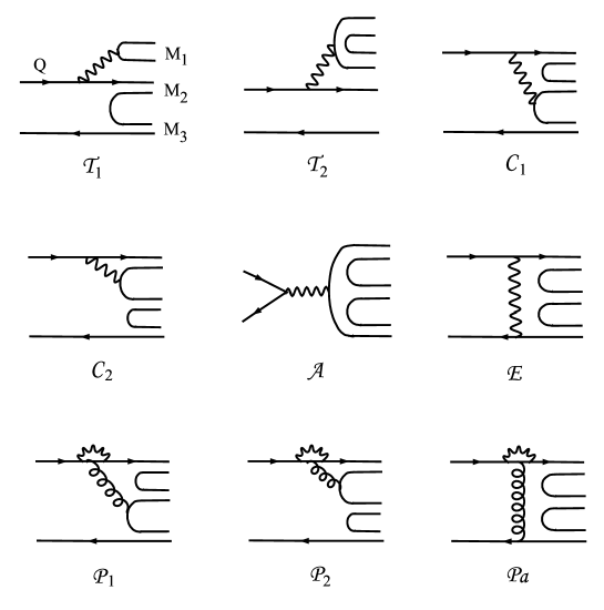
FIG. 2.: Quark diagrams for the three-body decays of heavy mesons, where $Q$ denotes a heavy quark.

The predicted branching ratios for direct charmless 3-body $B$ decays are shown in Table I. The decays $B^{-}\to\pi^{-}h^{+}h^{-}$ are tree dominated and their main contributions come from the $B^{*}$ pole. In contrast, the decays $B^{-}\to(K^{-}h^{+}h^{-})_{\rm NR}$ and $\overline{B}^{0}\to(\overline{K}^{0}h^{+}h^{-})_{\rm NR}$ for $h=\pi,K$ are penguin dominated. When $h=\pi$, the main contribution comes from the 2-body matrix elements of scalar densities, namely, the second term on the right hand side of Eq. (69), while the contribution from the three-body and one-body matrix elements of pseudoscalar densities [the first term of Eq. (69)] characterized by the term $2a_{6}m_{K}^{2}/(m_{b}m_{s})$ in Eq. (84) is largely compensated by the $a_{4}$ term.

Direct three-body charmless $B^{\pm}$ decays have been searched for by CLEO [26] with limits summarized in Table I. The decays $B^{-}\to\pi^{-}K^{+}K^{-},~{}K^{-}K^{+}K^{-}$ and $\overline{B}^{0}\to\overline{K}^{0}\pi^{+}\pi^{-},~{}\overline{K}^{0}K^{+}K^{-}$ were measured recently by Belle [19, 31] and BaBar [20] but without any assumptions on the intermediate states. It is interesting to note that the limits $1.2\times 10^{-5}$ set by Belle and $7\times 10^{-6}$ by BaBar for $\pi^{-}K^{+}K^{-}$ (resonant and nonresonant) is improved over the previous CLEO limit $7.5\times 10^{-5}$ for the nonresonant one. Needless to say, it is important to measure the nonresonant decay rates by $B$ factories and compare them with theory.

In the estimation of direct 3-body decay rates we have applied the $B^{*}BP$ strong coupling given by Eq. (28) and the $B^{*}\to P$ weak transition beyond their validity. Needless to say, this will cause some major theoretical uncertainties in the calculations because the strong $B^{*}BP$ coupling is derived under heavy quark and chiral symmetries and hence the momentum of the soft pseudoscalar should be less than $\Lambda_{\chi}$. For the energetic pseudoscalar, the intermediate $B^{*}$ state is far from its mass shell. It is assumed in [2] that the off-shellness of the $B^{*}$ pole is accounted for by replacing the term $\sqrt{m_{B^{*}}}$ in Eq. (28) by $(p_{B^{*}}^{2})^{1/4}$ and it is found that the branching ratios are reduced by $(30\sim 40)\%$ for $B^{-}\to\pi^{-}K^{+}K^{-},\pi^{+}\pi^{-}\pi^{-}$ as shown in Table I, while $B^{-}\to K^{-}h^{+}h^{-}$ for $h=\pi,K$ remain essentially unaffected. Using the measured branching ratios $(55.6\pm 5.8\pm 7.7)\times 10^{-6}$ and $(35.3\pm 3.7\pm 4.5)\times 10^{-6}$ by Belle [19], $(59.2\pm 4.7\pm 4.9)\times 10^{-6}$ and $(34.7\pm 2.0\pm 1.8)\times 10^{-6}$ by BaBar [20] for $B^{-}\to K^{-}\pi^{+}\pi^{-}$ and $B^{-}\to K^{-}K^{+}K^{-}$, respectively, in conjunction with the calculated results for direct 3-body decays, the corresponding fractions of nonresonant components are found to be 4% and 3%, respectively.

TABLE I.: Quark-diagram amplitudes and branching ratios for nonresonant 3-body charmless $B$ decays. The prediction ${\cal B}^{1}_{\rm theor}$ is made for $g_{BB_{(s)}^{*}K(\pi)}=2g/f_{\pi}\times(m_{B}m_{B_{(s)}^{*}})^{1/2}$ while the ${\cal B}^{2}_{\rm theor}$ accounts the off-shellness of the $B_{(s)}^{*}$ by letting $g_{BB_{(s)}^{*}K(\pi)}=2g/f_{\pi}\times\left(m_{B}\sqrt{p_{B_{(s)}^{*}}^{2}}\right)^{1/2}$. Experimental limits are taken from [31].

Decay mode	Quark-diagram amplitude	${\cal B}^{1}_{\rm theor}$	${\cal B}^{2}_{\rm theor}$	${\cal B}_{\rm expt}$ [32]
$B^{-}\to\pi^{-}\pi^{+}\pi^{-}$	$V_{ub}V_{ud}^{*}\sqrt{2}({\cal T}_{1}+{\cal C}_{1}+{\cal A})+V_{tb}V_{td}^{*}\sqrt{2}({\cal P}_{1}+{\cal P}_{2}+{\cal P}_{a})$	$3.0\times 10^{-6}$	$1.7\times 10^{-6}$	$<4.1\times 10^{-5}$
$\quad~{}\to\pi^{-}K^{+}K^{-}$	$V_{ub}V_{ud}^{*}({\cal T}_{1}+{\cal C}_{1}+{\cal A})+V_{tb}V_{td}^{*}({\cal P}_{1}+{\cal P}_{2}+{\cal P}_{a})$	$1.8\times 10^{-6}$	$1.3\times 10^{-6}$	$<7.5\times 10^{-5}$
$\quad~{}\to K^{-}\pi^{+}\pi^{-}$	$V_{ub}V_{us}^{*}({\cal T}_{1}+{\cal C}_{1}+{\cal A})+V_{tb}V_{ts}^{*}({\cal P}_{1}+{\cal P}_{2}+{\cal P}_{a})$	$2.4\times 10^{-6}$	$2.3\times 10^{-6}$	$<2.8\times 10^{-5}$
$\quad~{}\to K^{-}K^{+}K^{-}$	$V_{ub}V_{us}^{*}\sqrt{2}({\cal T}_{1}+{\cal C}_{1}+{\cal A})+V_{tb}V_{ts}^{*}\sqrt{2}({\cal P}_{1}+{\cal P}_{2}+{\cal P}_{a})$	$9.1\times 10^{-7}$	$8.5\times 10^{-7}$	$<3.8\times 10^{-5}$
$\overline{B}^{0}\to\overline{K}^{0}\pi^{+}\pi^{-}$	$V_{ub}V_{us}^{*}{\cal C}_{1}+V_{tb}V_{ts}^{*}({\cal P}_{1}+{\cal P}_{2}+{\cal P}_{a})$	$2.1\times 10^{-6}$	$2.1\times 10^{-6}$
$\quad~{}\to\overline{K}^{0}K^{+}K^{-}$	$V_{ub}V_{us}^{*}({\cal T}_{1}+{\cal C}_{1})+V_{tb}V_{ts}^{*}({\cal P}_{1}+{\cal P}_{2}+{\cal P}_{a})$	$1.2\times 10^{-6}$	$1.2\times 10^{-6}$

III Nonresonant three-body decays of $D$ mesons

For nonresonant three-body $D$ decays, the applicability of HMChPT should be in a better position than the $B$ meson case. In Table II the maximum momentum $p$ of any of the decay products in the $D$ rest frame is listed. As stressed in [17], $D\to KKK$ are the decay modes where HMChPT can be reliably applied since $p$ there is of order 545 MeV which is below the chiral symmetry breaking scale. For other $\overline{K}\pi\pi$ and $\overline{K}K\pi$ modes, the regime of the phase space where HMChPT is applicable is not necessarily small.

The calculations for nonresonant three-body decays of the charmed mesons proceed in the same way as the $B$ meson case and they are performed in the framework of HMChPT for two different cases: (i) HMChPT is applied to both strong and weak vertices, and (ii) it is applied only to the strong vertex and the weak transition is accounted for by form factors. These two different cases are denoted by ${\cal B}^{a}$ and ${\cal B}^{b}$, respectively, in Table II. Here we would like to point out some interesting physics. First, consider the decay $D^{0}\to\overline{K}^{0}\pi^{+}\pi^{-}$. In HMChPT its amplitude is given by

$$A(D^{0}\to\pi^{-}(p_{1})\overline{K}^{0}(p_{2})\pi^{+}(p_{3}))=-{G_{F}\over\sqrt{2}}V_{cs}V_{ud}^{*}(a_{1}A_{1}+a_{2}A_{2}),$$ (97)

with

$$A_{1} = {f_{\pi}\over 2}\left\{2m_{3}^{2}r+(m_{D}^{2}-s-m_{3}^{2})\omega_{+}+(2t+s-m_{D}^{2}-2m_{2}^{2}-m_{3}^{2})\omega_{-}\right\},$$ (98)

$$A_{2} = {f_{K}\over 2}\left\{2m_{2}^{2}r+(m_{D}^{2}-u-m_{2}^{2})\omega_{+}+(2t+u-m_{D}^{2}-2m_{3}^{2}-m_{2}^{2})\omega_{-}\right\},$$ (99)

where the form factors $r,~{}\omega_{+}$ and $\omega_{-}$ have similar expressions as Eq. (18). Since $a_{1}$ and $a_{2}$ in $D$ decays are opposite in signs [see Eq. (8)], it follows that the decay rate is suppressed owing to the destructive interference, see Table II.

However, when HMChPT is applied only to the strong vertex, the main contribution to $D^{0}\to\overline{K}^{0}\pi^{+}\pi^{-}$ comes from the $D^{*+}$ pole, namely, the strong process $D^{0}\to\pi^{-}D^{*+}$ followed by the weak transition $D^{*+}\to\overline{K}^{0}\pi^{+}$. Since it is known that the interference in $D^{+}\to\overline{K}^{0}\pi^{+}$ is destructive, naively it is expected that the same destructive interference occurs in the nonresonant $D^{0}\to\overline{K}^{0}\pi^{+}\pi^{-}$ decay. However, this is not the case. The $D^{*}$ pole amplitude is

$$A(D^{0}\to\overline{K}^{0}\pi^{+}\pi^{-})_{\rm pole} = A^{\mu}_{D^{*}\pi K}\,{i(-g_{\mu\nu}+p_{D^{*}\mu}p_{D^{*}\nu}/m_{D^{*}}^{2})\over p_{D^{*}}^{2}-m_{D^{*}}^{2}}\,A_{DD^{*}\pi}^{\nu}.$$ (100)

Now under factorization

$$\varepsilon_{\mu}A^{\mu}_{D^{*}\pi K}={G_{F}\over\sqrt{2}}V_{cs}V_{ud}^{*} \Big{\{} a_{1}\langle\pi^{+}(p_{3})|(\bar{u}d)_{{}_{V-A}}|0\rangle\langle\overline{K}^{0}(p_{2})|(\bar{s}c)_{{}_{V-A}}|D^{*+}(p_{D^{*}})\rangle$$ (101)

$$+ a_{2}\langle\overline{K}^{0}(p_{2})|(\bar{s}d)_{{}_{V-A}}|0\rangle\langle\pi^{+}(p_{3})|(\bar{u}c)_{{}_{V-A}}|D^{*+}(p_{D^{*}})\rangle\Big{\}}.$$ (102)

Applying heavy quark symmetry one can relate the form factors in $\langle\overline{K}^{0}|(\bar{s}c)_{{}_{V-A}}|D^{*+}\rangle$ to those in $\langle\overline{K}^{0}|(\bar{s}c)_{{}_{V-A}}|D^{+}\rangle$:

$$\langle\overline{K}^{0}(p_{K})|(\bar{s}c)_{{}_{V-A}}|D^{+}(p_{D})\rangle=f_{+}^{DK}(q^{2})(p_{D}+p_{K})_{\mu}+f_{-}^{DK}(q^{2})(p_{D}-p_{K})_{\mu}.$$ (103)

We obtain

$$\varepsilon_{\mu}A^{\mu}_{D^{*}\pi K}=-i{G_{F}\over\sqrt{2}}V_{cs}V_{ud}^{*}(\varepsilon\cdot p_{3}) \Bigg{\{} a_{1}\,f_{\pi}\Big{[}(f_{+}+f_{-})^{DK}m_{D}+(f_{+}-f_{-})^{DK}{t\over m_{D}}\Big{]}$$ (104)

$$- a_{2}\,f_{K}\Big{[}(f_{+}+f_{-})^{D\pi}m_{D}+(f_{+}-f_{-})^{D\pi}{t\over m_{D}}\Big{]}\Bigg{\}}.$$ (105)

It is interesting to note that although the interference is destructive in $D^{*+}\to\overline{K}^{0}\pi^{+}$, it becomes constructive in the process $D^{0}\to\pi^{-}D^{*+}\to\pi^{-}\pi^{+}\overline{K}^{0}$. We see from Table II that ${\cal B}^{b}$ is indeed much larger than ${\cal B}^{a}$ for $D^{0}\to\overline{K}^{0}\pi^{+}\pi^{-}$.

TABLE II.: Quark-diagram amplitudes and branching ratios (in percent) for nonresonant 3-body $D$ decays, where $p$ (in units of MeV) is the largest momentum any of the products can have in the $D$ rest frame. Heavy meson chiral perturbation theory is applied to both heavy-light strong and weak vertices for the theoretical prediction ${\cal B}^{a}$, while it is applied only to the strong vertex for ${\cal B}^{b}$. Form factors for $D\to\pi$ and $D\to K$ transitions are taken from [25] and experimental results from [31]. For the recent measurements of the nonresonant decays $D^{+}\to K^{-}\pi^{+}\pi^{+}$, $D^{0}\to\bar{K}^{0}K^{+}K^{-}$ and $D_{s}^{+}\to\pi^{+}\pi^{+}\pi^{-}$, see the text.

Decay mode	$p$	Quark-diagram amplitude	${\cal B}^{a}_{\rm theor}$	${\cal B}^{b}_{\rm theor}$	${\cal B}_{\rm expt}$ [32]
$D^{0}\to\overline{K}^{0}\pi^{+}\pi^{-}$	842	$V_{ud}V_{cs}^{*}({\cal T}_{1}+{\cal C}_{2}+{\cal E})$	0.03	0.17	see text
$\quad~{}\to K^{-}\pi^{+}\pi^{0}$	844	$V_{ud}V_{cs}^{*}{1\over\sqrt{2}}({\cal T}_{1}+{\cal C}_{1})$	0.61	0.28	$1.05^{+0.51}_{-0.19}$
$\quad~{}\to\overline{K}^{0}K^{+}K^{-}$	544	$V_{ud}V_{cs}^{*}({\cal T}_{2}+{\cal C}_{2}+{\cal E})$	0.16	0.01	$0.55\pm 0.09$
$D^{+}\to\overline{K}^{0}\pi^{+}\pi^{0}$	845	$V_{ud}V_{cs}^{*}{1\over\sqrt{2}}({\cal T}_{1}+{\cal C}_{1})$	1.5	0.7	$1.3\pm 1.1$
$\qquad\to K^{-}\pi^{+}\pi^{+}$	845	$V_{ud}V_{cs}^{*}\sqrt{2}({\cal T}_{1}+{\cal C}_{1})$	6.5	1.6	$8.6\pm 0.8$
$\qquad\to\pi^{+}\pi^{+}\pi^{-}$	908	$V_{ud}V_{cd}^{*}\sqrt{2}({\cal T}_{1}+{\cal C}_{1}+{\cal A}+{\cal P}_{1})+V_{us}V_{cs}^{*}\sqrt{2}({\cal P}_{1})$	0.50	0.067	$0.024\pm 0.021$
$\qquad\to K^{-}K^{+}\pi^{+}$	744	$V_{ud}V_{cd}^{*}({\cal A}+{\cal P}_{1})+V_{us}V_{cs}^{*}({\cal T}_{1}+{\cal C}_{1}+{\cal E})$	0.48	0.004	$0.45\pm 0.09$
$D_{s}^{+}\to K^{-}K^{+}\pi^{+}$	805	$V_{ud}V_{cs}^{*}({\cal T}_{1}+{\cal C}_{1}+{\cal A})$	1.0	0.69	$0.9\pm 0.4$
$\qquad\to\pi^{+}\pi^{+}\pi^{-}$	959	$V_{ud}V_{cs}^{*}\sqrt{2}({\cal A})$			$0.005\pm 0.022$

The nonresonant decay $D^{0}\to(\overline{K}^{0}K^{+}K^{-})_{\rm NR}$ deserves a special attention for two reasons. First, it is the only Cabibbo-allowed direct 3-body mode which receives contributions from the external $W$-emission diagram ${\cal T}_{2}$ (see Fig. 2). Second, as noted in passing, HMChPT is presumably most reliable for this mode. Its factorizable amplitude has the form

$$A(D^{0}\to K^{-}(p_{1})K^{+}(p_{2})\overline{K}^{0}(p_{3}))_{\rm NR} = {G_{F}\over\sqrt{2}}V_{ud}V_{cs}^{*}\Bigg{\{}a_{1}\langle K^{+}\overline{K}^{0}|(\bar{u}d)_{{}_{V-A}}|0\rangle\langle K^{-}|(\bar{s}c)_{{}_{V-A}}|D^{0}\rangle$$ (106)

$$+ a_{2}\langle\overline{K}^{0}|(\bar{s}d)_{{}_{V-A}}|0\rangle\langle K^{-}K^{+}|(\bar{u}c)_{{}_{V-A}}|D^{0}\rangle$$ (107)

$$+ a_{2}\langle K^{-}K^{+}\overline{K}^{0}|(\bar{s}d)_{{}_{V-A}}|0\rangle\langle 0|(\bar{u}c)_{{}_{V-A}}|D^{0}\rangle\Bigg{\}},$$ (108)

where the three terms on the right hand side correspond to the quark diagrams ${\cal T}_{2}$, ${\cal C}_{2}$ and ${\cal E}$, respectively. Proceeding as before and neglecting the $W$-exchange contribution in the chiral limit, we obtain

$$A(D^{0}\to K^{-}(p_{1})K^{+}(p_{2})\overline{K}^{0}(p_{3}))_{\rm NR}={G_{F}\over\sqrt{2}}V_{ud}V_{cs}^{*}\Big{\{}a_{1}A^{\prime}_{1}+a_{2}A^{\prime}_{2}\Big{\}},$$ (109)

where

$$A^{\prime}_{1} = {f_{D}\over f_{\pi}}\left\{{g\sqrt{m_{D}m_{D_{s}^{*}}^{3}}\over t-m_{D_{s}^{*}}^{2}}-{1\over 2}\right\}(s-u),$$ (110)

$$A^{\prime}_{2} = -{f_{K}\over 2}\left\{2m_{3}^{2}r+(m_{D}^{2}-s-m_{3}^{2})\omega_{+}+(2t+s-m_{D}^{2}-2m_{2}^{2}-m_{3}^{2})\omega_{-}\right\},$$ (111)

when HMChPT is applied to both strong and weak vertices, or

$$A^{\prime}_{1} = F_{1}^{DK}(t)F^{KK}(t)(s-u),$$ (112)

$$A^{\prime}_{2} = F_{1}^{D_{s}K}(m_{K}^{2}){g\sqrt{m_{D}m_{D_{s}^{*}}}\over t-m_{D_{s}^{*}}^{2}}\left[m_{D}+{t\over m_{D}}-m_{D}{m_{D}^{2}-t\over m_{K}^{2}}\left(1-{F_{0}^{D_{s}K}(m_{K}^{2})\over F_{1}^{D_{s}K}(m_{K}^{2})}\right)\right]$$ (113)

$$\times \left[s+t-m_{D}^{2}-m_{2}^{2}+{(t-m_{2}^{2}+m_{3}^{2})(m_{D}^{2}-t-m_{1}^{2})\over 2m_{D_{s}^{*}}^{2}}\right],$$ (114)

when HMChPT is applied only to the strong vertex. Again, the form factors $r$, $\omega_{+}$ and $\omega_{-}$ in Eq. (110) have the similar expressions as Eq. (18).

It is clear from Table II that the predicted branching ratio ${\cal B}^{a}$ of 0.16% for $D^{0}\to(\overline{K}^{0}K^{+}K^{-})_{\rm NR}$ works much better than ${\cal B}^{b}$, though the former is still too small compared to the experimental value $(0.55\pm 0.09)\%$ [32]. This decay was also considered by Zhang [17] within the same framework of HMChPT, but his result $2.3\times 10^{-4}$ for the branching ratio, which is similar to the prediction $2\times 10^{-4}$ based on chiral perturbation theory [12], is smaller than ours by one order of magnitude.

Some simple relations among different modes follow from the quark diagram approach. For example, neglecting the weak annihilation and penguin contributions and the phase space difference among different modes, it is expected that

$${{\cal B}(D^{+}\to\pi^{+}\pi^{+}\pi^{-})_{\rm NR}\over{\cal B}(D^{+}\to\pi^{+}\pi^{+}K^{-})_{\rm NR}} = \left|{V_{cd}\over V_{cs}}\right|^{2},$$ (115)

$${{\cal B}(D^{+}\to\overline{K}^{0}\pi^{+}\pi^{0})_{\rm NR}\over{\cal B}(D^{+}\to K^{-}\pi^{+}\pi^{-})_{\rm NR}} = {1\over 4},$$ (116)

$${{\cal B}(D^{+}\to K^{-}K^{+}\pi^{+})_{\rm NR}\over{\cal B}(D^{+}\to\pi^{+}\pi^{+}\pi^{-})_{\rm NR}} = {1\over 2},$$ (117)

$${{\cal B}(D_{s}^{+}\to K^{-}K^{+}\pi^{+})_{\rm NR}\over{\cal B}(D^{+}\to K^{-}\pi^{+}\pi^{+})_{\rm NR}} = {1\over 2}{\tau(D_{s}^{+})\over\tau(D^{+})}.$$ (118)

The above anticipation can be checked against the experimental results. It is easily seen that the measured $D^{+}\to(\pi\pi\pi)_{\rm NR}$ is too small compared to the theoretical prediction. For example, the observation that $(\pi^{+}K^{+}K^{-})_{\rm NR}\gg(\pi^{+}\pi^{+}\pi^{-})_{\rm NR}$ in $D^{+}$ decays is rather unexpected.

We see from Table II that the predictions for case (i) denoted by ${\cal B}^{a}$ are generally larger than case (ii) denoted by ${\cal B}^{b}$ except for the decay $D^{0}\to\overline{K}^{0}\pi^{+}\pi^{-}$. Contrary to the $B$ meson case where the predicted rates in these two different methods can differ by one to two orders of magnitude, ${\cal B}^{a}$ and ${\cal B}^{b}$ in some of $D$ decays differ only by a factor of 2. It is also evident that in general ${\cal B}^{b}$s give a better agreement with experiment for many of the direct 3-body $D$ decays , whereas ${\cal B}^{a}$ works better for $D^{0}\to\overline{K}^{0}K^{+}K^{-}$ and $D^{+}\to K^{-}K^{+}\pi^{+}$, though the prediction of the former mode by HMChPT is still too small compared to experiment. As noted in the Introduction, the early predictions based on SU(4) chiral perturbation theory are in general too small when compared with experiment [12, 13].

There exist several new measurements of direct 3-body $D$ decays in past few years: $D^{0}\to K^{-}\pi^{+}\pi^{0},~{}\overline{K}^{0}\pi^{+}\pi^{-},~{}\overline{K}^{0}K^{+}K^{-}$, $D^{+}\to\pi^{+}\pi^{+}\pi^{-},~{}K^{-}\pi^{+}\pi^{+}$ and $D_{s}^{+}\to\pi^{+}\pi^{+}\pi^{-}$. The nonresonant branching ratio for the first mode is found to be $(1.0\pm 0.1\pm 0.1^{+0.8}_{-0.1})\times 10^{-2}$ by CLEO [33]. Previous experiments [34] indicate that the decay $D^{+}\to K^{-}\pi^{+}\pi^{+}$ is strongly dominated by the nonresonant term with $(95\pm 7)\%$ [32]. However, a recent Dalitz plot analysis by E791 [35] reveals that a best fit to the data is obtained if the presence of an additional scalar resonance $\kappa$ is included. As a consequence, the nonresonant decay fraction drops from 95% to $(13\pm 6)\%$, whereas $\kappa\pi^{+}$ accounts for $(48\pm 12)\%$ of the total rate. Therefore, the branching ratio of the direct decay $D^{+}\to K^{-}\pi^{+}\pi^{+}$ is dropped from $(8.6\pm 0.8)\%$ to $(1.2\pm 0.6)\%$. Likewise, It was found by the E687 experiment that the decay $D^{+}\to\pi^{+}\pi^{+}\pi^{-}$ is dominated by the nonresonant contribution with $(60\pm 11)\%$ [36]. Again, the new Dalitz plot analysis by E791 [37] points out that half of the decays is accounted for by the scalar resonance $\sigma$, whereas the nonresonant fraction is only $(7.8\pm 6.0\pm 2.7)\%$. Consequently, ${\cal B}(D^{+}\to\pi^{+}\pi^{+}\pi^{-})_{\rm NR}$ drops to $(0.024\pm 0.021)\%$. Very recently BaBar has reported the preliminary result of the Dalitz plot analysis of $D^{0}\to\overline{K}^{0}K^{+}K^{-}$ [38]. Its nonresonant fraction is estimated to be $(0.4\pm 0.3\pm 0.8)\%$ and hence is negligible.

As for the direct decay $D^{0}\to\overline{K}^{0}\pi^{+}\pi^{-}$, the 2000 edition of Particle Data Group (PDG) [39] quotes a value of $(1.47\pm 0.24)\%$ for its branching ratio. However, it is no longer cited in the 2002 PDG [32] as no evidence for a nonresonant component is seen according to the most detailed analyses performed in [40]. This is also confirmed by a very recent CLEO measurement of this decay mode which gives $(0.9\pm 0.4^{+1.0+1.7}_{-0.3-0.2})\%$ for the nonresonant fraction [41].

The Cabibbo-suppressed decay $D_{s}^{+}\to(\pi^{+}\pi^{+}\pi^{-})_{\rm NR}$ proceeds only through the $W$-annihilation diagram. The early E691 measurement gives $R={\cal B}(D_{s}^{+}\to\pi^{+}\pi^{+}\pi^{-})_{\rm NR}/{\cal B}(D_{s}^{+}\to\phi\pi^{+})=0.29\pm 0.09\pm 0.03$ [42]. However, it was found to be negligible by E791 [43] and its branching ratio is quoted to be $(5\pm 22)\times 10^{-5}$ by 2002 PDG (see Table II). Recently, FOCUS has reported the preliminary result: the nonresonant fraction is measured to be $(25.5\pm 4.6)\%$ [44]. This corresponds to ${\cal B}(D_{s}^{+}\to\pi^{+}\pi^{+}\pi^{-})_{\rm NR}=(2.6\pm 0.9)\times 10^{-3}$. Although the short-distance $W$-annihilation vanishes in the chiral limit, the long-distance one can be induced from final-state rescattering (see e.g. [46]). Therefore, the observation of direct $D_{s}^{+}\to\pi^{+}\pi^{+}\pi^{-}$ implies the importance of final-state interactions for nonresonant decays.

IV Conclusions

We have presented a systematical study of nonresonant three-body decays of $D$ and $B$ mesons. We first draw some conclusions from our analysis and then proceed to discuss the sources of theoretical uncertainties during the course of calculation.

1. It is pointed out that if heavy meson chiral perturbation theory (HMChPT) is applied to the heavy-light strong and weak vertices and assumed to be valid over the whole kinematic region, then the predicted decay rates for nonresonant 3-body $B$ decays will be too large and especially $B^{-}\to\pi^{-}K^{+}K^{-}$ exceeds substantially the current experimental limit. This can be understood because chiral symmetry has been applied twice beyond its region of validity.

2. If HMChPT is applied only to the strong vertex and the weak transition is accounted for by the form factors, the dominant $B^{*}$ pole contribution to the tree-dominated direct three-body $B$ decays will become small and the branching ratio will be of order $10^{-6}$. The decay modes $B^{-}\to(K^{-}h^{+}h^{-})_{\rm NR}$ and $\overline{B}^{0}\to(\overline{K}^{0}h^{+}h^{-})_{\rm NR}$ for $h=\pi,K$ are penguin dominated.

3. We have considered the use of HMChPT in two different cases to study the direct 3-body $D$ decays. We found that when HMChPT is applied only to the strong vertex, the predictions in general give a better agreement with experiment except for the decays $D^{0}\to K^{-}\pi^{+}\pi^{0},\overline{K}^{0}K^{+}K^{-}$ and $D^{+}\to K^{-}K^{+}\pi^{+}$ where a full use of HMChPT to the weak vertices gives a better description. The $D^{*+}$ pole contribution to $D^{0}\to\overline{K}^{0}\pi^{+}\pi^{-}$ proceeds through external and internal $W$-emission diagrams with constructive interference. The experimental observation that $(\pi^{+}K^{+}K^{-})_{\rm NR}\gg(\pi^{+}\pi^{+}\pi^{-})_{\rm NR}$ in $D^{+}$ decays is largely unanticipated.

It is useful to summarize the theoretical uncertainties encountered in the present paper, though most of them have been discussed before:

• For $B^{*}$ (and also $D^{*}$) pole contributions, the intermediate state $B^{*}$ is off its mass shell when the pseudoscalar meson coupled to $B^{*}$ and $B$ is no longer soft. This will affect the $B^{*}BP$ strong coupling. To estimate the off-shell effect of $B^{*}$, we replace its mass $m_{B^{*}}$ by $\sqrt{p_{B^{*}}^{2}}$ and find that the branching ratios for $B^{-}\to\pi^{-}K^{+}K^{-},\pi^{+}\pi^{-}\pi^{-}$ are reduced by $(30\sim 40)\%$, while $B^{-}\to K^{-}\pi^{+}\pi^{-},K^{-}K^{+}K^{-}$ remain essentially unaffected.

• We have parametrized the $q^{2}$ dependence of the form factors $F^{\pi\pi}_{\rm nonres},F^{KK}_{\rm nonres}$, $F^{K\pi}_{\rm nonres}$ and $F^{K\pi\pi}$ in the form of Eqs. (94), (95) and (96). However, part of scalar resonance effects is included in the parametrization of the form factors. In the $B$ decays, the major uncertainty of the calculated amplitudes comes from the chiral enhanced term $\sim F_{0,{\rm nonres}}^{K\pi}(2a_{6}-a_{8})\times m_{B}(m_{K}^{2}-m_{\pi}^{2})/m_{s}$. We may overestimate the penguin-dominant nonresonant branching ratios if there exist scalar resonances, e.g. $\kappa$. Although in some channels the $\sigma$ resonance is included in $F^{\pi\pi}_{\rm nonres}$, its effect is suppressed by the Cabibbo angle and by the fact that it decouples to the vector current in the SU(2) symmetry limit.

• The point-like contact contribution to the three-body matrix element beyond the chiral limit, e.g. $\langle P_{1}P_{2}|(\bar{q}b)_{{}_{V-A}}|B\rangle_{\rm contact}$, is unknown but it becomes even smaller when $P_{1}$ or $P_{2}$ is not soft owing to the smaller wave function overlap among $P_{1},P_{2}$ and $B$. Therefore it can be neglected in our calculations.

• Thus far we have assumed the factorization approximation to evaluate the decay amplitudes. It is known in the QCD factorization approach [47] that factorization is justified in the heavy quark limit where power corrections of order $1/m_{B}$ and $1/m_{D}$ can be neglected. Beyond the heavy quark limit, factorization is violated by power corrections which in general cannot be systematically explored. Nevertheless, some of them are calculable. For example, in the $B$ decays we have included the terms proportional to $a_{6}$ and $a_{8}$ which are of order $\bar{\Lambda}/m_{b}$ but chirally enhanced. Final-state interactions which have been neglected so far are also of order $\bar{\Lambda}/m_{Q}$. The decay $D_{s}^{+}\to(\pi^{+}\pi^{+}\pi^{-})_{\rm NR}$ proceeds only through the $W$-annihilation process. Even if the short-distance contribution to the weak annihilation vanishes, it may receive sizable long-distance contributions via final-state rescattering. The preliminary FOCUS measurement of this mode may provide the first indication of the importance of final-state interactions for the weak annihilation process in nonresonant $D$ decays. A precise measurement of this mode can test the validity of the applying the factorization picture to the nonresonant three-body decays.

- [1]
- [2] N.G. Deshpande, G. Eilam, X.G. He, and J. Trampetić, Phys. Rev. D52, 5354 (1995).
- [3] S. Fajfer, R.J. Oakes, and T.N. Pham, Phys. Rev. D60, 054029 (1999).
- [4] B. Bajc, S. Fajfer, R.J. Oakes, T.N. Pham, and S. Prelovsek, Phys. Lett. B447, 313 (1999).
- [5] A. Deandrea, R. Gatto, M. Ladisa, G. Nardulli, and P. Santorelli, Phys. Rev. D62, 036001 (2000); ibid. 62, 114011 (2000).
- [6] A. Deandrea and A.D. Polosa, Phys. Rev. Lett. 86, 216 (2001).
- [7] J. Tandean and S. Gardner, hep-ph/0204147.
- [8] I. Bediaga, C. Göbel, and R. Méndez-Galain, Phys. Rev. D56, 4268 (1997).
- [9] P. Singer, Phys. Rev. D16, 2304 (1977); Nuovo Cim. 42A, 25 (1977).
- [10] Yu. L. Kalinovsk and V.N. Pervushin, Sov. J. Nucl. Phys. 29, 225 (1979).
- [11] H.Y. Cheng, Z. Phys. C32, 243 (1986).
- [12] L.L. Chau and H.Y. Cheng, Phys. Rev. D41, 1510 (1990).
- [13] F.J. Botella, S. Noguera, and J. Portolés, Phys. Lett. B360, 101 (1995).
- [14] T.M. Yan, H.Y. Cheng, C.Y. Cheung, G.L. Lin, Y.C. Lin, and H.L. Yu, Phys. Rev. D46, 1148 (1992); 55, 5851(E) (1997).
- [15] M.B. Wise, Phys. Rev. D45, 2118 (1992).
- [16] G. Burdman and J.F. Donoghue, Phys. Lett. B280, 287 (1992).
- [17] D.X. Zhang, Phys. Lett. B382, 421 (1996).
- [18] A.N. Ivanov and N.I. Troitskaya, Nuovo Cim. A111, 85 (1998).
- [19] Belle Collaboration, A. Garmash et al., Phys. Rev. D65, 092005 (2002).
- [20] BaBar Collaboration, B. Aubert et al., hep-ex/0206004.
- [21] D.S. Du, H. Gong, J. Sun, D. Yang, and G. Zhu, Phys. Rev. D65, 094025 (2002).
- [22] S. Fajfer, R.J. Oakes, and T.N. Pham, Phys. Lett. B539, 67 (2002).
- [23] C.L.Y. Lee, M. Lu, and M.B. Wise, Phys. Rev. D46, 5040 (1992).
- [24] H.Y. Cheng, Int. J. Mod. Phys. A4, 495 (1989).
- [25] CLEO Collaboration, A. Anastassov et al., Phys. Rev. D65, 032003 (2002).
- [26] CLEO Collaboration, T. Bergfeld et al., Phys. Rev. Lett. 77, 4503 (1996).
- [27] M. Wirbel, B. Stech, and M. Bauer, Z. Phys. C29, 637 (1985); M. Bauer, B. Stech, and M. Wirbel, ibid. C34, 103 (1987).
- [28] D. Melikhov and B. Stech, Phys. Rev. D62, 014006 (2001).
- [29] H. Georgi, Weak Interactions and Modern Particle Theory (Benjamin/Cummings, New York, 1984).
- [30] L.L. Chau and H.Y. Cheng, Phys. Rev. D36, 137 (1987); Phys. Lett. B222, 285 (1989).
- [31] Belle Collaboration, talk presented by H.C. Huang at XXXVIIth Rencontres de Moriond Electroweak Interactions and Unified Theories (9 - 16 March 2002, Les Arcs, France).
- [32] Particle Data Group, K. Hagiwara et al., Phys. Rev. D66, 010001 (2002).
- [33] CLEO Collaboration, S. Kopp et al., Phys. Rev. D63, 092001 (2001).
- [34] E687 Collaboration, P.L. Frabetti et al., Phys. Lett. B331, 217 (1994); E691 Collaboration, J.C. Anjos et al., Phys. Rev. D48, 56 (1993); Mark III Collaboration, J. Adler et al., Phys. Lett. B191, 318 (1987).
- [35] E791 Collaboration, E.M. Aitala et al., hep-ex/0204018.
- [36] E687 Collaboration, P.L. Frabetti et al., Phys. Lett. 407, 79 (1997).
- [37] E791 Collaboration, E.M. Aitala et al., Phys. Rev. Lett. 86, 770 (2001).
- [38] BaBar Collaboration, B. Aubert et al., hep-ex/0207089.
- [39] Particle Data Group, D.E. Groom et al., Eur. Phys. J. C15, 1 (2000).
- [40] P.L. Frabetti et al., Phys. Lett. B331, 217 (1994); H. Albrecht et al., ibid. B308, 435 (1993).
- [41] CLEO Collaboration, H. Muramatsu et al., hep-ex/0207067.
- [42] E691 Collaboration, J.C. Anjos et al., Phys. Rev. Lett. 62, 125 (1989).
- [43] E791 Collaboration, E.M. Aitala et al., Phys. Rev. Lett. 86, 765 (2001).
- [44] FOCUS Collaboration, talk presented by S. Erba at the DPF Meeting of the American Physical Society at Williamsburgh, Virginia, May 24-28, 2002.
- [45] N.L. Hoang, A.V. Nguyen, and X.Y. Pham, Phys. Lett. B357, 177 (1995).
- [46] H.Y. Cheng, hep-ph/0202254.
- [47] M. Beneke, G. Buchalla, M. Neubert, and C.T. Sachrajda, Nucl. Phys. B591, 313 (2000).