LBNL-50169

UCB-PTH-02/19

hep-ph/0204315

April 26, 2002

Heterotic Orbifolds

Joel Giedt

Department of Physics, University of California,
and Theoretical Physics Group, 50A-5101,
Lawrence Berkeley National Laboratory, Berkeley, CA 94720 USA.

Abstract

A review of orbifold geometry is given, followed by a review of the construction of four-dimensional heterotic string models by compactification on a six-dimensional $Z_{3}$ orbifold. Particular attention is given to the details of the transition from a classical theory to a first-quantized theory. Subsequently, a discussion is given of the systematic enumeration of all standard-like three generation models subject to certain limiting conditions. It is found that the complete set is described by 192 models, with only five possibilities for the hidden sector gauge group. It is argued that only four of the hidden sector gauge groups are viable for dynamical supersymmetry breaking, leaving only 175 promising models in the class. General features of the spectra of matter states in all 175 models are discussed. Twenty patterns of representations are found to occur. Accomodation of the Minimal Supersymmetric Standard Model (MSSM) spectrum is addressed. States beyond those contained in the MSSM and nonstandard hypercharge normalization are shown to be generic, though some models do allow for the usual hypercharge normalization found in $SU(5)$ embeddings of the Standard Model gauge group. Only one of the twenty patterns of representations, comprising seven of the 175 models, is found to be without an anomalous $U(1)$. Various quantities of interest in effective supergravity model building are tabulated for the set of 175 models. String scale gauge coupling unification is shown to be possible, albeit contrived, in an example model.

Prefatory Remarks

What follows is my doctoral thesis. Its purpose is two-fold. First, I review “well-known” aspects of orbifold geometry and its application to the weakly-coupled heterotic string. These are the contents of Chapters 1-2. Second, I describe my own research, the emphasis of which has been the construction of semi-realistic $Z_{3}$ heterotic orbifold models within a restricted class. This material is contained in Chapters 3-5 and is based on my two recent articles [1, 2].

I have written Chapter 1 to be elementary and accessible to a wide audience. It is my hope that it might prove useful to those who are just beginning a study of orbifolds. I was able to do this because the topic is fairly self-contained and does not require a large amount of preparatory knowledge beyond that already possessed by most graduate students in theoretical physics or mathematics.

Chapter 2 is best supplemented with standard texts on string theory, say, the first volume of Green, Schwarz and Witten [3]. Moreover, Chapter 2 assumes familiarity with the theory of Lie algebras and groups, especially the Cartan system of roots and weights. The review of string theoretic aspects of heterotic orbifold theory is somewhat heuristic. I would have preferred to have given a complete and self-contained discussion rather than what the reader will find in Chapter 2. However, after attempting this project, I gradually began to understand that such an endeavor would—if properly done—encompass a rather large book! Therefore, I have resorted to the more “poetic” presentation of Chapter 2, supplementing it with adequate references to the several very good reviews and texts which are widely available. Thus, the intent of Chapter 2 is to provide the reader with a general impression of the approach taken to building semi-realistic string theories, and to introduce crucial terms within a context which provides, hopefully, an intuitive sense of their meanings.

Does string theory have anything to do with the material universe? It is questionable whether or not we will ever have compelling evidence which would indicate the answer to this question. I do not expect string theory to ever stand on the same experimental footing as, say, the Standard Model of elementary particle physics.

If an affirmative answer is forthcoming, I believe it will probably come from the application of string theory to strongly coupled Quantum Chromodynamics (QCD), where string-like behavior has already been “observed” in quark confinement, the Regge trajectories of the hadron spectrum, and in Lattice Gauge Theory simulations of the confining phase of QCD.

However, the application of string theory to QCD is not the topic of this thesis. Rather, the line of research taken up here envisions string theory as an underlying theory behind all of the fundamental interactions between elementary particles observed in the laboratory. The energy scale where the “stringy” nature of the underlying theory really becomes apparent is many orders of magnitude beyond the reach of particle accelerators, at least in the case of the weakly-coupled heterotic string. Optimistically, a few distinctive “stringy” remanants might possibly be observed in, say, searches for fractionally charged particles, or (very optimistically) ultra-high energy cosmic ray experiments.

The real advantage to string theory is not that it provides hard and fast predictions for experimental observations which are just around the corner. (It does however constrain what might be observed.) Rather, its chief strength is in its (perhaps unique) ability to provide resolutions to troubling theoretical difficulties. I will discuss these in the Motivations section which follows. Given that it apparently resolves these difficulties, it is important to determine whether it can simultaneously accomodate our view of the material universe. Can it consistently account for what is observed? This has been the main focus of my research. Another important question to answer is the following. If string theory is the underlying theory of the interactions of elementary particles, in what ways does it limit effective theories describing what will be observed in the coming years? This is the topic of “stringy” constraints on physics beyond the Standard Model of elementary particle physics. My research also touches on this question.

At this point I remark that the universe is larger than the material universe! For instance, there is the universe of ideas, abstract structures and mathematics without any apparent applications. Regardless of the suitability of string theory for the description of aspects of the material universe, it is a description of fascinating mathematical structures. As such, I would like to find a vehicle to communicate my studies to the mathematical community. There are numerous difficulties, however, in doing so. Foremost among these is a difference in language. For instance, physicists talk about “fields” while mathematicians talk about “sections of fiber bundles.” Bridging this gap is no small task, due to the years of specialized training in separate departments of the academy. I had originally thought to provide enough elementary discussions, footnotes and appendices to render this thesis accessible to non-physicists. I eventually determined that the goal was not terribly realistic, as I would have to learn quite a bit more mathematics than I had time to do in the final year of my doctoral program and because the amount of theoretical physics material that I would have to review was going to be a great quantity.

Consequently, I am afraid that I have had to resort to an appendix which outlines a few good references which a person could read to become sufficiently familiar with the terminology, techniques and models of modern particle theory. These references review these topics better than I ever could, and I recommend that readers interested in better understanding this thesis consider reading them concurrently, at least poetically.

Motivations${}^{\hbox{{\rm\normalsize*}}}$

The quantum theory of fields provides an adequate description of the electromagnetic, weak and strong interactions; to these gauge interactions, one may add the mass interactions of quarks and leptons, including “mass-mixing” interactions such as those which appear in the charged current. For a variety of reasons, it is widely believed that new particles and interactions beyond those now known may soon be detected in precision low-energy experiments and “next generation” high-energy colliders. Moreover, quantized field theory with its point-like interactions runs into difficulties in two rather significant respects. First, it allows for the spontaneous emission and reabsorption of particles which are “off mass-shell,” $E^{2}\not={\bf p}^{2}+m^{2}$, where $m$ is the measured mass. These “virtual” particles yield quantum corrections to the interactions and field strengths (the normalization of fields) of quarks and leptons which are often infinite. The usual response to this is to point out that it is only the quantum corrected field strengths and interaction strengths (measured by coupling parameters) which are physically meaningful, since in an experimental process we always measure quantities which have all quantum effects included. Thus, the original, uncorrected “bare” field strengths and coupling parameters are not fundamental, and should be adjusted such that the infinities which arise from quantum corrections are canceled when we compute (infrared safe) rates, lifetimes and other physical processes. The systematic implementation of this philosophy goes by the name renormalization. In order to cancel the infinities, they must be rendered finite by imposing a cutoff of some kind; this taming of infinities is known as regularization.

The game of regularization and renormalization is perfectly capable of rendering quantum field theory a successful calculation tool for describing and predicting observed processes. Indeed, the program has proven quite a triumph in the cases of quantum electrodynamics, the electroweak theory and weakly coupled QCD, as well as a mixed success in the description of hadrons and their interactions. However, many physicists are unsatisfied with this state of affairs and seek to understand the infinities which arise and how they might be avoided. When one studies the effects of the virtual particles, it is found that the infinites may be traced back to the contribution of virtual particles with very large energies or momenta; these are the ultraviolet divergences of quantized field theories. The most naive way to regularize a typical quantum field theory is to impose an artificial cutoff on the energies and momenta of virtual particles. One may imagine that the particle content and interactions of a theory has a limited range of validity, depending on energy and momentum scales. One can further posit that the quantum field theory used to calculate the effects of virtual particles is beyond its range of validity in precisely that region where the effects become disturbingly large. This would explain why bizarre results are obtained in the calculation of quantum corrections: we have gone beyond the limitations of our theory. The question then becomes, what is the correct theory at these higher energies and momenta? I will refer to this as the underlying theory.

The underlying theory must satisfy certain requirements. First, it must have as its low energy limit a quantized theory of fields which includes quarks and leptons and their interactions. Second, it must be finite; that is, we want a theory where artificial cutoffs are no longer necessary and where ultraviolet behavior is “softened” in a natural way. Third, it must provide a quantum description of gravity. Remarkably, a theory exists which is believed to possess all of these properties! Actually, a few exist, all string theories of one brand or another. However, they are all thought to be limits of a more fundamental theory—the mysterious M-theory. In this work, I shall chiefly be concerned with the weakly coupled heterotic string theory [5]. In its original construction, this is a theory with ten space-time dimensions. The non-observation of spatial dimensions other than the three of the everyday world suggests that the six extra dimensions, should they really exist, be hidden from us in some way.

The oldest way to accomplish this goes back to Kaluza-Klein theory [6], where extra dimensions are made very small and compact. Difficulties arise in obtaining chiral fermions in the effective four-dimensional theory. These difficulties were surmounted at the field theory level by Chapline et al. [7] through compactification on quotient manifolds. Shortly after the invention of the heterotic string, Candelas et al. illustrated how compactification of this type of string on a Calabi-Yau manifold could produce an effective theory with local ${\it N=1}$ supersymmetry and chiral fermions in four dimensions [8]. However, Calabi-Yau manifolds pose technical difficulties for the explicit calculation of many important quantities in the effective theory. Concurrent to the intiation of the Calabi-Yau studies, Dixon, Harvey, Vafa and Witten showed how to use of a certain class of quotient spaces—orbifolds—to build more calculable four-dimensional string models [9, 10]. Orbifolds are Euclidean except at a finite number of points. This is a great simplification over Calabi-Yau manifolds. Since the six-dimensional orbifolds studied in this context may be viewed as singular limits of certain Calabi-Yau manifolds, we can presume that many of the more important features of these manifolds can be understood in this orbifold limit. A comparison of quantities which can be calculated in both theories bears out the validity this presumption.

Orbifold compactifications of heterotic string theory are of interest because many aspects of the theory are tractable and because they can generate realistic models. Like Calabi-Yau manifolds, orbifolds can generate local ${\it N=1}$ supersymmetry in four dimensions. Supersymmetry protects the hierarchy between the Planck scale ($m_{P}=1/\sqrt{8\pi G}=2.44\times 10^{18}$ GeV, where $G$ is Newton’s gravitational coupling) and the electoweak scale ($m_{Z}=91.19$ GeV, where this is the mass of the Z boson); in a non-supersymmetric theory we would expect this hierarchy to be destabilized by the effects of virtual particles. $N=1$ supersymmetry is desirable to accomodate the standard model, a chiral theory with particles which lie in complex representations of gauge groups. Local supersymmetry is required in order to have a realistic mass spectrum for the states beyond those contained in the Standard Model (SM), the superpartners to the quarks, leptons and gauge bosons. This is because a realistic spectrum may only be obtained by so-called soft supersymmetry breaking in the low energy effective theory, which is achieved by the spontaneous breaking of local supersymmetry in an effective supergravity theory valid at higher energies.

In this thesis, I will restrict my attention to the $Z_{3}$ orbifold, which is often referred to simply as “the $Z$ orbifold.” It is the canonical example and has been studied extensively, yet many of the more detailed issues of this construction of a four-dimensional heterotic theory remain uninvestigated. Several aspects of the $Z_{3}$ orbifold make it simpler than other orbifold constructions. To explain these would require jargon which will be defined below; I will not enumerate them here but will note these simplifying features as they arise in the discussion which follows.

Chapter 1 Orbifold geometry

In this chapter I discuss the geometry of orbifolds. I begin in Section 1.1 with a very simple (and currently popular) example, the one-dimensional orbifold. Next, I look at the two-dimensional case in Section 1.2. Finally, I arrive in Section 1.3 at the orbifold which will concern us throughout the remainder of this work, the $Z_{3}$ orbifold. Thus I build gradually to the six-dimensional construction, so that key concepts are introduced in simpler one- and two-dimensional examples.

1.1 One-dimensional Orbifold

I begin with the simplest orbifold that can be constructed. It provides an introduction to some of the concepts, terminology and notation common to the discussion of orbifolds.

Let ${{\bf R}}$ be the real number line. Define a one-dimensional lattice $\Lambda$ with lattice spacing $a\in{{\bf R}}$:

$$\Lambda=\left\{\;na\;|\;n\in{{\bf Z}}\;\right\},$$ (1.1)

where ${{\bf Z}}$ is the set of integers. The elements $\ell\in\Lambda$ will be referred to as lattice vectors. We construct a torus by identifying points on the line with each other if they are related under addition by a lattice vector:

$$x\simeq x+\ell\qquad\forall\;x\in{{\bf R}},\,\ell\in\Lambda.$$ (1.2)

This generates a torus whose fundamental domain can be chosen as $[0,a)$. That is, any other point in ${{\bf R}}$ maps into this domain by the identification made in (1.2); ${{\bf R}}$ is the covering space for the torus.

For example, the points labeled “x” in Figure 1.1 are equivalent on the torus. The one-dimensional torus is topologically equivalent (more precisely, homeomorphic) to a circle. We notate this construction

$${{\bf T}}={{\bf R}}/\Lambda.$$ (1.3)

The torus ${{\bf T}}$ is compact while the real number line ${{\bf R}}$ is non-compact.

An “active attitude” may be taken: Eq. (1.2) states that points which are related to each other by a lattice vector translation are equivalent to each other. The discrete group of translations defined by the lattice is referred to as the lattice group, which is often also denoted $\Lambda$. The lattice group is an invariance or isometry group of ${{\bf R}}$. This terminology leads to a brief description of the torus construction: we “divide out” or “mod out” the lattice group $\Lambda$ from the space ${{\bf R}}$. The lattice group affords an equivalence relation $r_{\Lambda}$, defined by (1.2), which partitions the real number line into a set of equivalence classes; an equivalence class is a set of elements which are all equivalent to each other. The set of equivalence classes is called the quotient set or quotient space determined by $r_{\Lambda}$ and is denoted by ${\bf R}/r_{\Lambda}$. However, most people use the shorthand ${\bf R}/\Lambda$, as in (1.3). Since ${{\bf R}}$ and $\Lambda$ are groups, it is also correct to refer to ${\bf R}/\Lambda$ as a coset space. Each element in the fundamental domain $[0,a)$ is in one-to-one correspondence with an equivalence class contained in ${\bf R}/\Lambda$. Given $x\in[0,a)$ we can reach (generate) every element in the equivalence class corresponding to $x$ by the action of the lattice group $\Lambda$ on $x$.

Figure 1.1: The torus ${{\bf T}}$ embedded into the covering space ${{\bf R}}$.

A toroidal orbifold may be constructed from a torus by supplementing (1.2) with other equivalence relations. A twist operator is used to define each equivalence relation. For the toroidal orbifolds considered here, the twist must be an automorphism of the lattice used in constructing the torus. An automorphism $\theta$ of a lattice $\Lambda$ is a transformation which maps lattice vectors into lattice vectors:

$$\theta\ell\in\Lambda,\qquad\forall\;\ell\in\Lambda.$$ (1.4)

Twist operators are most often generators of a discrete rotation group on the compact manifold which is to be “twisted” into an orbifold, typically a torus.

In the simplified one-dimensional case that I present here, rotation is not well defined. Instead, I take the twist operator to be the parity operator ${\bf P}$:

$${{\bf P}}x=-x,\qquad\forall\;x\in{{\bf R}}.$$ (1.5)

The parity operation is an automorphism of the lattice $\Lambda$ since it satisfies (1.4). It is very simple to see that this is the case. Any lattice vector may be written as $na$, where $n$ is an integer and $a$ is the lattice spacing. Applying the parity operation,

$${{\bf P}}(na)=-(na)=(-n)a.$$ (1.6)

But since $-n$ is also an integer, it can be seen that the right-hand side of (1.6) is a lattice vector of $\Lambda$ too.

The equivalence relation generated by ${\bf P}$ is

$$x\simeq{\bf P}x,\,\qquad\forall\;x\in{\bf R}.$$ (1.7)

Notice that ${\bf P}^{2}=1$. Thus, ${\bf P}$ realizes the cyclic group of order two, commonly referred to as $Z_{2}$. The group generated by the twist operators is known as the point group of the orbifold. We then have as the point group for our simple one-dimensional orbifold

$$Z_{2}=\{1,{{\bf P}}\}.$$ (1.8)

The orbifold we have constructed, denoted $\Omega(1,Z_{2})$, is the quotient space ${{\bf T}}/Z_{2}$.

It is very common to define operators which combine the action of the point group $Z_{2}$ with the lattice group $\Lambda$:

$$(\omega,\ell)x=\omega x+\ell,\qquad\forall\;x\in{{\bf R}},$$ (1.9)

where $\omega\in Z_{2},\;\ell\in\Lambda$. The collection of all such operators forms a group $S$ known as the space group of the orbifold. It is not difficult to check that these operators have the multiplication rule

$$(\omega_{1},\ell_{1})(\omega_{2},\ell_{2})=(\omega_{1}\omega_{2},\ell_{1}+\omega_{1}\ell_{2}).$$ (1.10)

An isomorphism of the point group is a bijective map $g$ which satisfies

$$g(\omega_{1})g(\omega_{2})=g(\omega_{1}\omega_{2}).$$ (1.11)

Similarly an isomorphism of the lattice group is a bijective map $h$ which satisfies

$$h(\ell_{1})h(\ell_{2})=h(\ell_{1}+\ell_{2}).$$ (1.12)

The projection of the space group onto the point group defined by

$$\pi_{1}(\omega,\ell)\cdot x=\omega x,\qquad\forall\;x\in{{\bf R}},$$ (1.13)

is a homomorphism to the point group, as can be seen from (1.10). On the other hand the projection of the space group onto the lattice group defined by

$$\pi_{2}(\omega,\ell)\cdot x=x+\ell,\qquad\forall\;x\in{{\bf R}},$$ (1.14)

is not a homorphism to the lattice group. From (1.10) we have

$$\pi_{2}((\omega_{1},\ell_{1})(\omega_{2},\ell_{2}))\cdot x=x+\ell_{1}+\omega_{1}\ell_{2},\qquad\forall\;x\in{{\bf R}},$$ (1.15)

whereas

$$\left(\pi_{2}(\omega_{1},\ell_{1})\circ\pi_{2}(\omega_{2},\ell_{2})\right)\cdot x=x+\ell_{1}+\ell_{2},\qquad\forall\;x\in{{\bf R}}.$$ (1.16)

For this reason, the space group is the semi-direct product of the point group and the lattice group.

We have so far constructed the one-dimensional orbifold in a two step process, imposing the equivalence (1.2) and then equivalence (1.7). The space group $S$ affords a more compact description:

$$x\simeq gx,\qquad\forall\;x\in{{\bf R}},\;g\in S.$$ (1.17)

The orbifold may be denoted $\Omega(1,Z_{2})={{\bf R}}/S$.

Figure 1.2: The orbifold ${\bf T}/Z_{2}$ and its embedding into the covering space ${{\bf R}}$. Points marked with the same letter are equivalent.

In Figure (1.2) I illustrate the orbifold. All points marked with the same letter are equivalent. Note that in the fundamental domain $[0,a)$ of the torus we now have pairs of points which are equivalent, except for the fixed points $x=0$ and $x=a/2$. (A proper definition of fixed points will be given below.) On the other hand, the fundamental domain of the orbifold is $[0,a/2]$, for every other point in ${{\bf R}}$ may be mapped into this interval.

Note that we can “fit” a local one-dimensional coordinate system, commonly referred to as the tangent space, at points $w$ and $y$. However, things become confused at the fixed points, such as $z$. On the covering space, both directions leaving $z$ are equivalent; we cannot fit a well-defined tangent space in the neighborhood of $z$. This “difficulty” is a general feature of orbifold fixed points; it distinguishes orbifolds from manifolds.

One may imagine folding the fundamental domain $[0,a)$ of the torus at $x=a/2$ and bending it back over so the two half-segments overlap and the ends of the fundamental domain touch, as shown in Figure 1.3. Points which overlap are equivalent.

Figure 1.3: Fold the fundamental domain of the one-dimensional torus to form the one-dimensional orbifold. Points which overlap are equivalent.

The torus may be pictured as an ellipse in the two-dimensional plane. We may think of the orbifold construction as an ellipse whose eccentricity ${\epsilon}$ is taken to the limit ${\epsilon}\to 1$ (the minor axis approaches vanishing length relative to the length of the major axis) while the length of the major axis is held fixed; see Figure 1.4. Thus, we can no longer resolve the “top” of the ellipse from the “bottom.” The points $x=0$ and $x=a/2$ coincide with the ends of the major axis in this picture, and one can see intuitively that they are in a certain sense singular.

Figure 1.4: Ellipse collapsing to segment under identification.

Specifically, let us consider motion on the ellipse which covers the orbifold. In the vicinity of the fixed points, the corresponding motion on the orbifold has an interesting behavior. Keeping the ellipse with shrinking minor axis in mind, we imagine parallel transporting a vector about the fixed point, which has been marked by an “x” in the Figure 1.5. The starting and ending orientations are indicated. On the orbifold, the starting point and the ending point are equivalent. Thus, the path is a closed “loop” on our singular space. It can be seen that from the orbifold perspective, the vector has undergone a rotation $\Delta\theta=\pi$ as one passes “around” the fixed point. This is independent of how small a loop we take. The curvature $\kappa(s)$ of a curve is the magnitude of the rate of change in the unit tangent vector ${\bf T}(s)$ with respect to path length $s$:

$$\kappa(s)=\left|{d{\bf T}(s)\over ds}\right|.$$ (1.18)

About the fixed point we have

$$\kappa\propto\lim_{\Delta s\to 0}{\Delta\theta\over\Delta s}=\lim_{\Delta s\to 0}{\pi\over\Delta s}=\infty.$$ (1.19)

We see that the fixed point is a point of infinite curvature. An orbifold is not a manifold because of the existence of curvature singularities at the fixed points.

Figure 1.5: Parallel transport about a fixed point in the one-dimensional orbifold leads to a rotation by $\pi$, regardless of how small the loop becomes. Curvature at the fixed point is infinite.

Let us examine these points in greater detail and see in what sense they are “fixed.” Note first that ${{\bf P}}x=x$ if $x=0$. That is, $x=0$ is neutral under the action of the point group. Next note that

$${{\bf P}}(a/2)=-a/2=a/2-a,$$ (1.20)

so that ${{\bf P}}(a/2)\simeq a/2$ under the action of the lattice group, (1.2). This leads us to the general definition of a fixed point. Let $\omega$ be an element of the point group of an orbifold. Then a fixed point of the operator $\omega$ is a solution $x_{f}$ to

$$\omega x_{f}+\ell=x_{f},$$ (1.21)

with $\ell$ some element of the lattice $\Lambda$.

Example 1.1

The points $x=0$ and $x=a/2$ are the fixed points contained in the fundamental domain of our orbifold. $\Box$

All other fixed points (integral and half-integral multiples of $a$) are equivalent to one of these two fixed points under the action of the lattice group. In this sense, our orbifold has “two” fixed points; the correct statment is that the orbifold possesses precisely two inequivalent fixed points. Note that (1.21) may be written more succinctly as neutrality with respect to a space group element:

$$(\omega,\ell)\cdot x_{f}=x_{f}.$$ (1.22)

Through (1.22) each pair $(\omega,\ell)$ can be put into one-to-one correspondence with an element $x_{f}$ of the covering space ${{\bf R}}$. Each of these elements is a fixed point of the twist operator $\omega$ on the orbifold. That is to say, given a pair $(\omega,\ell)$, the solution $x_{f}\in{{\bf R}}$ to (1.22) is unique and always exists.

Example 1.2

In Example 1.1, we saw that the fixed point $x_{f}=0$ corresponded to the lattice vector $\ell=0$ while the fixed point $x_{f}=a/2$ corresponded to the lattice vector $\ell=a$. $\Box$

More generally,

$$({{\bf P}},na){n\over 2}a={n\over 2}a,\qquad\forall\;n\in{{\bf Z}}.$$ (1.23)

Thus, the fixed point $na/2$ corresponds to the lattice vector $na$. Since all fixed points with $n$ even are equivalent to $x_{f}=0$, this fixed point corresponds to the sublattice spanned by lattice vectors $na$ with $n$ even. Similarly, the fixed point $x_{f}=a/2$ corresponds to the sublattice spanned by lattice vectors $na$ with $n$ odd.

1.2 Two-dimensional Orbifold

The next example is a generalization of the last. We extend to the two-dimensional real manifold ${{\bf R}}^{2}$ and mod out by a lattice generated by linearly independent elements $e_{1},e_{2}\in{{\bf R}}$:

$$\Lambda=\left\{\;\sum_{i=1}^{2}m^{i}e_{i}\;\left|\;m^{1},m^{2}\in{\bf Z}\;\right.\right\}$$ (1.24)

The basis vectors characterize the shape and size of the lattice via

$$\sqrt{e_{1}\cdot e_{1}}=a_{1},\qquad\sqrt{e_{2}\cdot e_{2}}=a_{2},\qquad e_{1}\cdot e_{2}=a_{1}a_{2}\cos\alpha.$$ (1.25)

The torus described by ${{\bf T}}^{2}={{\bf R}}^{2}/\Lambda$ is obtained by imposing equivalence relations

$$x\simeq x+\ell,\qquad\forall\;x\in{{\bf R}}^{2},\,\ell\in\Lambda.$$ (1.26)

We again define the twist operator to be the parity operation ${{\bf P}}\cdot x=-x$ and impose the identification

$$x\simeq{\bf P}\cdot x\,\qquad\forall\;x\in{{\bf T}}^{2}$$ (1.27)

to construct the orbifold $\Omega(2,Z_{2})={{\bf T}}^{2}/Z_{2}$. We note that ${{\bf P}}$ is equivalent to a rotation by angle $\pi$. Thus, the point group is a discrete subgroup of the full rotation group $O(2)$ of the real manifold ${{\bf R}}^{2}$; this is the usual circumstance in toroidal orbifolds, and will be true in the six-dimensional $Z_{3}$ case considered in Section 1.3. It is easy to check that (1.27) is an automorphism of the lattice (1.24). As discussed in the one-dimensional example of Section 1.1 this is a necessary condition for the consistency of the orbifold construction.

Figure 1.6: The orbifold ${\bf T}^{2}/Z_{2}$, for the special case of $a_{1}=a_{2},\,\alpha=0$. Points marked with the same letter are equivalent. The fundamental region of the torus is $[0,1)\times[0,1)$. Four fixed points exist in this region, marked by solid dots.

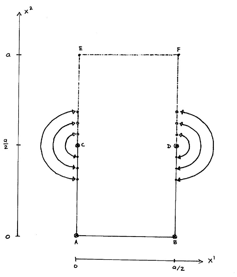
Figure 1.7: ${\cal F}$ for the $Z_{2}$ orbifold. Open points along the open boundary (dotted) are identified (examples shown by arrows) with closed points along the closed boundary (solid), forming a “pillow.”

The orbifold, embedded into the covering space ${{\bf R}}^{2}$, is depicted in Figure 1.6 for the special case of $a_{1}=a_{2}\equiv a,\,\alpha=0$. Locating equivalent points is now a bit more complicated, but with a brief study one can convince oneself that points labeled with the same letter are related—by a combination of operations (1.26,1.27). With a bit more effort, one should be able to convince oneself that a valid choice for the fundamental domain ${\cal F}\subset{{\bf R}}^{2}$ of the orbifold is

$${\cal F}=[0,a/2]\times[0,a/2]+(0,a/2)\times(a/2,a).$$ (1.28)

The notation here specifies a sum of two squares $M_{1}\times M_{2}$, where $M_{1}$ is an interval parallel to the $x^{1}$-axis and $M_{2}$ is and interval parallel to the $x^{2}$-axis. For greater clarity, this choice of ${\cal F}$ is shown in Figure 1.7. The limit points along the open boundary are identified with points on the closed boundary as indicated by arrows. That is: ${\overline{AC}}$ is sewn to ${\overline{CE}}$; ${\overline{AB}}$ is sewn to ${\overline{EF}}$; and, ${\overline{BD}}$ is sewn to ${\overline{DF}}$. This is done such that $A$ and $E$ connect, as do $B$ and $F$. Thus on the orbifold the edges are sewn together about $x^{2}=a/2$ to form a four-cornered “pillow.” The space is clearly compact, and has four “corners” where the space looks locally like a cone; at each one of these corners there is a point where the curvature is singular. These four conical singularities are the fixed points of the orbifold: $A,\,B,\,C$ and $D$.

These four inequivalent fixed points can also be found by the algebraic method. It is easy to check that (using the space group notation)

$$({{\bf P}},m^{i}e_{i}){m^{j}e_{j}\over 2}={m^{j}e_{j}\over 2}$$ (1.29)

for all pairs of integers $(m^{1},m^{2})$. Thus, the fixed points of the orbifold are given by $m^{i}e_{i}/2$. The lattice vectors given by

$$(m^{1},m^{2})\in\{(0,0),\;(0,1),\;(1,0),\;(1,1)\}$$ (1.30)

give fixed points $m^{i}e_{i}/2$ which are inequivalent to each other and which are related to all other fixed points by a lattice group equivalence (1.26).

1.3 The Six-dimensional ${\bf Z_{3}}$ Orbifold

Toroidal orbifolds of dimension larger than those so far considered are mere generalizations of the two-dimensional construction just described. However, the increase in dimensionality allows for many more possibilities. We will be concerned with six-dimensional orbifolds in the applications considered in subsequent chapters. This is because the heterotic string theory, as originally formulated, has nine spatial dimensions. To construct an effective theory with only the three spatial dimensions we observe, it is necessary to somehow hide the extra six. The standard approach to this is to make the six extra dimensions compact and very small—a characteristic length on the order of $8\times 10^{-33}$ centimeters! For reasons which will be explained in later chapters, promising models follow from the assumption that the six-dimensional compact space is an orbifold. In this thesis I concentrate on the possibility that it is a $Z_{3}$ orbifold.

1.3.1 Construction

The six-dimensional $Z_{3}$ orbifold may be constructed from a six-dimensional Euclidean space ${{\bf R}}^{6}$. One defines basis vectors $e_{1},\ldots,e_{6}$ satisfying

$$e_{i}^{2}=e_{i+1}^{2}=2R_{i}^{2},\qquad e_{i}\cdot e_{i+1}=-1R_{i}^{2},\qquad i=1,3,5,$$ (1.31)

with a vector $x\in{{\bf R}}^{6}$ having real-valued components:

$$x=\sum_{i=1}^{6}x^{i}e_{i},\qquad x^{i}\in{{\bf R}}\quad\forall\;i=1,\ldots,6.$$ (1.32)

Note that $x^{i}\not=x\cdot e_{i}$ since the root basis (1.31) is a skew basis consisting of elements which do not have unit norm. Each of the three pairs $e_{i},e_{i+1}\;(i=1,3,5)$ define a two-dimensional subspace which is referred to below as the “$i$th complex plane.” The $i$th such pair also defines a two-dimensional $SU(3)$ root lattice, obtained from the set of all linear combinations of the form $n_{i}e_{i}+n_{i+1}e_{i+1}$ with $n_{i},n_{i+1}$ both integers. Taking together all six basis vectors $e_{1},\ldots,e_{6}$, we obtain the $SU(3)^{3}$ root lattice ${\Lambda_{SU(3)^{3}}}$, formed from all linear combinations of the basis vectors $e_{1},\ldots,e_{6}$ with integer coefficients:

$${\Lambda_{SU(3)^{3}}}=\left\{\left.\;\sum_{i=1}^{6}\ell^{i}e_{i}\;\right|\;\ell^{i}\in{{\bf Z}}\;\right\}.$$ (1.33)

Note that the radii $R_{i}$ in (1.31) are not fixed; neither are angles not appearing in (1.31), such as $e_{1}\cdot e_{3}$. These free parameters determine the size and shape of the unit cell of the lattice ${\Lambda_{SU(3)^{3}}}$, and are encoded in Kähler- or T-moduli $T^{ij}$. These moduli depend on the metric $G_{ij}=e_{i}\cdot e_{j}$ ($i,j=1,\ldots,6$) of the six-dimensional compact space, as well as an antisymmetric two-form $B_{ij}$. Of particular interest are the diagonal T-moduli $T^{i}\equiv T^{ii}$. Up to normalization conventions on the $T^{i}$ and $B_{ij}$, the diagonal T-moduli are defined by

$$T^{i}=\sqrt{\det G^{(i)}}+iB_{i,i+1},\quad i=1,3,5.$$ (1.34)

Here, $G^{(i)}$ is the metric of the $i$th complex plane:

$$G^{(i)}=\pmatrix{e_{i}\cdot e_{i}&e_{i}\cdot e_{i+1}\cr e_{i+1}\cdot e_{i}&e_{i+1}\cdot e_{i+1}\cr}=R_{i}^{2}\pmatrix{2&-1\cr-1&2\cr}.$$ (1.35)

Translations in ${{\bf R}}^{6}$ by elements of ${\Lambda_{SU(3)^{3}}}$,

$$x\to x+\ell,\qquad\ell\in{\Lambda_{SU(3)^{3}}},\qquad\forall\;x\in{{\bf R}}^{6},$$ (1.36)

form the lattice group; thus we obtain the six-dimensional torus ${{\bf T}}^{6}={{\bf R}}^{6}/{\Lambda_{SU(3)^{3}}}$. A suitable choice for the fundamental domain of this torus in any one of the three complex planes is given by the parallelogram ${\overline{DEAFD}}$ of Figure 1.8. (The interpretation of the figure is more transparent in terms of the complex basis which will be introduced in Section 1.3.3 below.)

The twist operator $\theta$ is a simultaneous $2\pi/3$ rotation of each of the three complex planes. Its action on the basis vectors is

$$\theta\cdot e_{i}=e_{i+1},\qquad\theta\cdot e_{i+1}=-e_{i}-e_{i+1},\qquad i=1,3,5.$$ (1.37)

It is easy to check that $\theta^{3}=1$. The twist operator $\theta$ generates the orbifold point group,

$$Z_{3}=\{1,\theta,\theta^{2}\}.$$ (1.38)

It can be seen from (1.37) that the twist operator maps any element of ${\Lambda_{SU(3)^{3}}}$ into ${\Lambda_{SU(3)^{3}}}$. Consequently, we can define the product group generated by the combined action of the point group and the lattice group— the space group $S$. As in the one- and two-dimensional examples considered above, a generic element is written $(\omega,\ell)$, with $\omega\in Z_{3}$ and $\ell\in{\Lambda_{SU(3)^{3}}}$. The space group has four generators: $(\theta,0),\;(1,e_{1}),\;(1,e_{3})$ and $(1,e_{5})$.

Example 1.3

Using (1.37) and the space group multiplication rule (1.10) one can write

$$(1,e_{2})=(\theta,0)\cdot(1,e_{1})\cdot(\theta,0)\cdot(\theta,0).$$ (1.39)

$\Box$

Acting on any element $x\in{{\bf R}}^{6}$,

$$(\omega,\ell)\cdot x=\omega\cdot x+\ell=\sum_{i=1}^{6}[x^{i}(\omega\cdot e_{i})+\ell^{i}e_{i}],$$ (1.40)

where $\omega\cdot e_{i}$ can be obtained by (repeated) application of (1.37).

Example 1.4

The pure twist element $(\theta,0)$ transforms $x\in{{\bf R}}^{6}$ according to

$$\theta\cdot x=\sum_{i=1,3,5}\left[x^{i}e_{i+1}-x^{i+1}(e_{i}+e_{i+1})\right]=\sum_{i=1,3,5}\left[-x^{i+1}e_{i}+(x^{i}-x^{i+1})e_{i+1}\right].$$ (1.41)

We can express the action of $\theta$ in terms of components by $x\to\theta\cdot x=x^{\prime}$ with

$$x^{i}\to(x^{\prime})^{i}=-x^{i+1},\qquad x^{i+1}\to(x^{\prime})^{i+1}=x^{i}-x^{i+1},\qquad i=1,3,5.$$ (1.42)

The difference between the coefficients in (1.37) versus (1.42) is due to the fact that the root basis is a skew basis. Eq. 1.42 leads to a matrix for the action of $\theta$ on the components:

$$M(\theta)=\mathop{{\hbox{diag}\,}}\nolimits[m(\theta),m(\theta),m(\theta)],\qquad m(\theta)=\pmatrix{0&-1\cr 1&-1\cr}.$$ (1.43)

$\Box$

Having described the space group, we define the six-dimensional $Z_{3}$ orbifold.

Definition 1.1

The orbifold $\Omega(6,Z_{3})={{\bf R}}^{6}/S$ is the quotient space constructed when we deem the points $x,x^{\prime}\in{{\bf R}}^{6}$ equivalent if they are related to each other under the action of the space group $S$: $x^{\prime}\simeq x$ if and only if there exists an element $(\omega,\ell)\in S$ such that $x^{\prime}=(\omega,\ell)\cdot x$.

A suitable fundamental domain for the orbifold, projected into any one of the three complex planes, is depicted in Figure 1.8. Sewing of open boundaries to closed boundaries is suggested by the arrows. Whereas in the two-dimensional $Z_{2}$ orbifold of Section 1.2 could be pictured as a four-cornered “pillow,” we now obtain for the $Z_{3}$ orbifold a three-cornered “pillow.” Since the orbifold is six-dimensional, we actually have three such pillow spaces associated with the projection of the orbifold into each of the three complex planes.

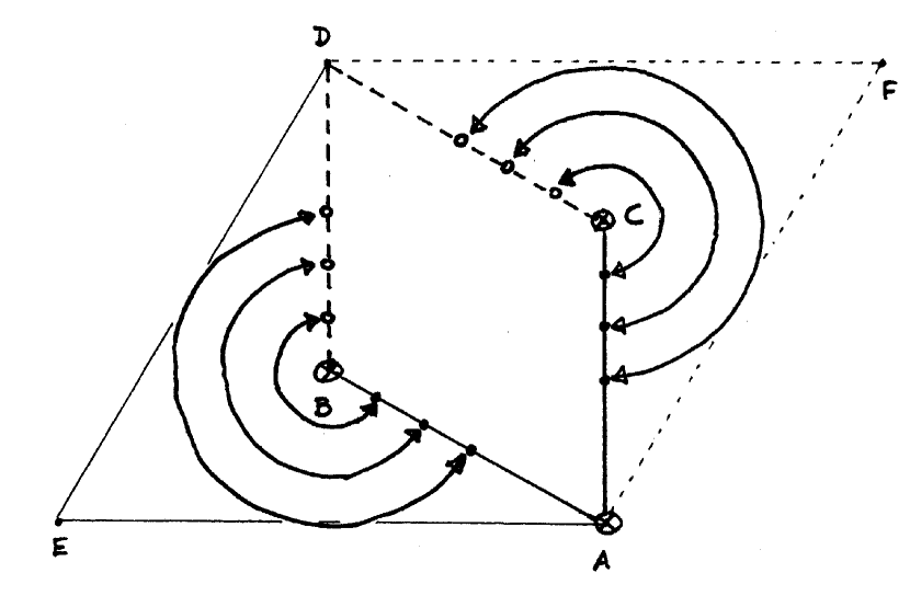
Figure 1.8: The parallelogram ${\overline{BACDB}}$ depicts the two-dimensional $Z_{3}$ orbifold. Also shown is how it sits within the $SU(3)$ root torus (the larger parallelogram). Here I take $E=0$, $A=1$, $D=e^{i\pi/3}$, $F=A+D$, $B=F/3$ and $C=2F/3$. Open points along the open boundary (dashed) are identified (examples shown by arrows) with closed points along the closed boundary (solid), forming a three-cornered “pillow.” The fixed points are at $A$, $B$ and $C$. We can also view the parallelogram ${\overline{BACDB}}$ as the projection of the six-dimensional $Z_{3}$ orbifold into one of the three complex planes. Similarly, the larger parallelogram can be viewed as the projection of the $SU(3)^{3}$ root torus in one of the three complex planes.

1.3.2 Conjugacy Classes and Fixed Points

The conjugacy class associated with the space group element $(\omega,\ell)$ is the set

$$\left\{\;(\omega^{\prime},\ell^{\prime})\cdot(\omega,\ell)\cdot(\omega^{\prime},\ell^{\prime})^{-1}\quad\left|\quad(\omega^{\prime},\ell^{\prime})\in S\;\right.\right\},$$ (1.44)

This partition of the space group is of prime importance in the application of the six-dimensional $Z_{3}$ orbifold to the heterotic string, as will be seen in Section 2.2 below. It will be useful to have a full determination of the conjugacy classes of space group. This is provided by the following examples.

Example 1.5

Let us consider the conjugacy class associated with a space group element which is a pure lattice translation $(1,\ell_{0})$. First note that the space group multiplication rule (1.10) implies

$$(\omega,\ell)^{-1}=(\omega^{-1},-\omega^{-1}\ell).$$ (1.45)

Again using (1.10) it is easy to check that

$$(\omega,\ell)(1,\ell_{0})(\omega,\ell)^{-1}=(1,\omega\ell_{0}).$$ (1.46)

Thus, in the case of the $Z_{3}$ orbifold where only three choices of $\omega$ are available (cf. Eq. (1.38)), the conjugacy class associated with $(1,\ell_{0})$ is given by

$$\{(1,\ell_{0}),(1,\theta\ell_{0}),(1,\theta^{2}\ell_{0})\}.$$ (1.47)

$\Box$

Example 1.6

Now I determine the conjugacy class associated with a twisted space group element $(\theta,\ell_{0})$.

$$(\omega,\ell)(\theta,\ell_{0})(\omega,\ell)^{-1} = (\omega\theta,\omega\ell_{0}+\ell)(\omega^{-1},-\omega^{-1}\ell)$$ (1.48)

$$= (\omega\theta\omega^{-1},-\omega\theta\omega^{-1}\ell+\omega\ell_{0}+\ell)$$

$$= (\theta,(1-\theta)\ell+\omega\ell_{0}).$$

In the last step I have used the fact that the point group $Z_{3}$ is abelian.

To begin with, consider $\omega=1$. It is not hard to check that

$$\ell\equiv\sum_{i=1}^{6}\ell^{i}e_{i}\quad\Rightarrow\quad(1-\theta)\ell=\sum_{i=1}^{6}\ell^{i}v_{i},$$

$$v_{i}\equiv e_{i}-e_{i+1},\quad v_{i+1}\equiv e_{i}+2e_{i+1},\quad i=1,3,5.$$ (1.49)

Then within the conjugacy class of $(\theta,\ell_{0})$ are all elements of the form

$$(\theta,\ell_{0}+\sum_{i=1}^{6}m^{i}v_{i})$$ (1.50)

with $m^{i}\in{{\bf Z}}$. Note that I have relabeled $\ell^{i}\to m^{i}$.

For $\omega=\theta$ we have

$$(\theta,(1-\theta)\ell+\omega\ell_{0})=(\theta,(1-\theta)\ell+\theta\ell_{0})=(\theta,(1-\theta)(\ell-\ell_{0})+\ell_{0}).$$ (1.51)

Without loss of generality we can take $\ell^{\prime}\equiv\ell-\ell_{0}$. Then we again obtain the same set of elements as for the $\omega=1$ case above, with $(\ell^{\prime})^{i}\equiv m^{i}$ in (1.50).

For $\omega=\theta^{2}$ we have

$$(\theta,(1-\theta)\ell+\omega\ell_{0})=(\theta,(1-\theta)\ell+\theta^{2}\ell_{0})=(\theta,(1-\theta)(\ell-\theta\ell_{0}-\ell_{0})+\ell_{0}).$$ (1.52)

Without loss of generality we can take $\ell^{\prime}\equiv\ell-\theta\ell_{0}-\ell_{0}$. We obtain the same set of elements, with $(\ell^{\prime})^{i}\equiv m^{i}$ in (1.50).

Therefore the conjugacy class of $(\theta,\ell_{0})$ is given by

$$\{(\theta,\ell_{0}+\sum_{i=1}^{6}m^{i}v_{i})\}_{m^{i}\in{{\bf Z}}}.$$ (1.53)

$\Box$

I now show that there are 27 inequivalent classes and that each class is labeled by a class leader of the form

$$\ell(n_{1},n_{3},n_{5})=n_{1}e_{1}+n_{3}e_{3}+n_{5}e_{5},\qquad n_{i}=0,\pm 1.$$ (1.54)

First suppose given the lattice vector $k=\sum_{i=1}^{6}k^{i}e_{i}$ and look for a solution to

$$k=\ell(n_{1},n_{3},n_{5})+\sum_{i=1}^{6}m^{i}v_{i}=\sum_{i=1,3,5}[n_{i}e_{i}+m^{i}(e_{i}-e_{i+1})+m^{i+1}(e_{i}+2e_{i+1})].$$ (1.55)

It is not hard to check that this leads to constraints equivalent to $(i=1,3,5)$:

$$3m^{i+1} = k^{i}+k^{i+1}-n_{i}$$ (1.56)

$$m^{i} = k^{i}-n_{i}-m^{i+1}$$ (1.57)

So first pick $n_{i}=0,\pm 1$ such that a solution $m^{i+1}\in{{\bf Z}}$ exists for the first equation—one of these three values of $n_{i}$ will always work. Then plug these values into the second equation to determine $m^{i}$. This shows that all lattice vectors can be written in the form (1.55). Now I show that the leaders belong to different classes.

Suppose $\ell(n_{1},n_{3},n_{5})$ and $\ell(n_{1}^{\prime},n_{3}^{\prime},n_{5}^{\prime})$ are in the same class. Then we can take $k\to\ell(n_{1}^{\prime},n_{3}^{\prime},n_{5}^{\prime})$ in (1.55) above. Eq. (1.56) gives $(i=1,3,5)$:

$$3m^{i+1}=n_{i}^{\prime}-n_{i}.$$ (1.58)

Because $n_{i}$ and $n_{i}^{\prime}$ take only values $0,\pm 1$, the only solution is $m^{i+1}=0$ and $n_{i}^{\prime}=n_{i}$. Therefore if $\ell(n_{1},n_{3},n_{5})$ and $\ell(n_{1}^{\prime},n_{3}^{\prime},n_{5}^{\prime})$ belong to the same class, they are identical to each other. Q.E.D.

As was the case for the one- and two-dimensional orbifolds discussed in Sections 1.1 and 1.2, certain points $x_{f}\in{{\bf R}}^{6}$ are fixed under the action of space group elements with $\omega=\theta$:

$$(\theta,\ell)\cdot x_{f}=\theta\cdot x_{f}+\ell=x_{f}.$$ (1.59)

It is not hard to solve this equation; one finds that the fixed points are in one-to-one correspondence with elements of ${\Lambda_{SU(3)^{3}}}$:

$$x_{f}(\ell)=(1-\theta)^{-1}\cdot\ell.$$ (1.60)

Because of the identification of points under $S$ on the orbifold, most of the fixed points (1.60) are equivalent to each other. In fact, only 27 inequivalent fixed points exist, and they are in one-to-one correspondence with the conjugacy class leaders (1.54), by way of (1.60):

$$f_{n_{1},n_{3},n_{5}}\equiv x_{f}(\ell(n_{1},n_{3},n_{5}))=(1-\theta)^{-1}\cdot\ell(n_{1},n_{3},n_{5}).$$ (1.61)

It is not difficult to prove these statements. The key steps of the proof are outlined in the following examples.

Example 1.7

Consider two fixed points corresponding to lattice vectors $\ell_{a}$ and $\ell_{b}$ in the same conjugacy class. Then from the considerations of Example 1.53 we know that there exist $m^{i}\in{{\bf Z}}$ such that

$$\ell_{b}=\ell_{a}+\sum_{i=1}^{6}m^{i}v_{i},$$ (1.62)

where the notation is as in (1.53). Furthermore, we found in Example 1.53 that the lattice vector $\ell$ defined by $\ell^{i}\equiv m^{i}$ satisfies

$$\sum_{i=1}^{6}m^{i}v_{i}=(1-\theta)\ell.$$ (1.63)

Then the corresponding fixed points, given by (1.60), are related by

$$x_{f}(\ell_{b})=(1-\theta)^{-1}[\ell_{a}+(1-\theta)\ell]=x_{f}(\ell_{a})+\ell.$$ (1.64)

Thus, fixed points corresponding to lattice vectors in the same twisted conjugacy class differ by a lattice vector; they are therefore equivalent on the orbifold. $\Box$

Example 1.8

In this example I show that the fixed points $x_{f}(0)=0$ and $x_{f}(e_{1})=(1-\theta)^{-1}e_{1}$ are not related by a lattice vector. By similar arguments it is easy to check that each of the 27 fixed points given in (1.61) are inequivalent.

Suppose $x_{f}(e_{1})\simeq x_{f}(0)$. Then there exists a lattice vector $\ell=\ell^{1}e_{1}+\ell^{2}e_{2}$ such that

$$(1-\theta)^{-1}e_{1}=\ell\quad\Rightarrow\quad e_{1}=(1-\theta)\ell=(\ell^{1}+\ell^{2})e_{1}+(2\ell^{2}-\ell^{1})e_{2}.$$ (1.65)

It is easy to check that linear independence of $e_{1}$ and $e_{2}$ then requires $3\ell^{2}=1$, which cannot be satisfied for $\ell^{2}\in{{\bf Z}}$. Thus we arive at a contradiction. $\Box$

1.3.3 The Complex Basis

For the applications in the following chapter, the root basis employed in (1.32) is inconvenient. Rather, we use a complex basis which is defined in terms of the components $x^{i}$ appearing in (1.32) according to

$$z^{i}\equiv x^{i}+e^{2\pi i/3}x^{i+1},\qquad{\bar{z}}^{i}\equiv x^{i}+e^{-2\pi i/3}x^{i+1},\qquad i=1,3,5.$$ (1.66)

This is motivated by supposing that in the $i$th complex plane $e_{i}$ lies along the real axis while from (1.31) we see that $e_{i+1}$ lies at 120 degrees counterclockwise from the real axis; i.e., along $e^{2\pi i/3}$. This picture is of course the origin of the usage of “complex plane” for each of the three pairs $e_{i},e_{i+1}$ ($i=1,3,5$).

From (1.42) it is not hard to show that the twist operator acts on $z^{i}$ as a pure phase rotation ($i=1,3,5$):

$$z^{i}\to(z^{\prime})^{i}=(x^{\prime})^{i}+e^{2\pi i/3}(x^{\prime})^{i+1}=e^{2\pi i/3}\left(x^{i}+e^{2\pi i/3}x^{i+1}\right)=e^{2\pi i/3}z^{i}.$$ (1.67)

Similarly,

$${\bar{z}}^{i}\to({\bar{z}}^{\prime})^{i}=e^{-2\pi i/3}{\bar{z}}^{i}.$$ (1.68)

In the complex basis, the matrix realization (1.43) is given instead by

$$M_{c}(\theta)=\mathop{{\hbox{diag}\,}}\nolimits(e^{2\pi i/3},e^{2\pi i/3},e^{2\pi i/3})$$ (1.69)

when acting on $(z^{1},z^{3},z^{3})$ and is the complex conjugate $[M_{c}(\theta)]^{*}$ when acting on vectors in the conjugate representation space $({\bar{z}}^{1},{\bar{z}}^{3},{\bar{z}}^{3})$. It is this decomposition into irreducible representations—no mixing between $z^{i}$ and ${\bar{z}}^{i}$, in contrast to the mixing between $x^{i}$ and $x^{i+1}$ in (1.43)—which eases manipulations when we come to applications below. The $Z_{3}$ nature of the point group is obvious from (1.69). It is the generator of the center of $SU(3)$ in the fundamental representation.

In an abuse of notation I shall often write $\theta=e^{2\pi i/3}$, so that (1.69) becomes

$$M_{c}(\theta)=\mathop{{\hbox{diag}\,}}\nolimits(\theta,\theta,\theta).$$ (1.70)

Furthermore, I collect the components (1.66) into a three-tuple ${{\bf z}}=(z^{1},z^{3},z^{5})$ and write the twist action (1.67) as

$${{\bf z}}\to{{\bf z}}^{\prime}=\theta{{\bf z}},$$ (1.71)

where $\theta$ here simply means scalar multiplication by $e^{2\pi i/3}$. It is also clear from (1.66) that the complex parameterization of a lattice vector $\ell$ takes the form

$$b^{i}(\ell)\equiv\ell^{i}+e^{2\pi i/3}\ell^{i+1},\qquad\bar{b}^{i}(\ell)\equiv\ell^{i}+e^{-2\pi i/3}\ell^{i+1},\qquad i=1,3,5.$$ (1.72)

Thus the action of a general space group element $(\omega,\ell)$ with $\omega=\theta^{n}$ ($n=0,\pm 1$) is given by

$${{\bf z}}\to{{\bf z}}^{\prime}=(\theta^{n},\ell){{\bf z}}=\theta^{n}{{\bf z}}+{{\bf b}}(\ell)=e^{2n\pi i/3}{{\bf z}}+{{\bf b}}(\ell),$$ (1.73)

where ${{\bf b}}=(b^{1},b^{3},b^{5})$. The correspondence (1.60) between fixed points and lattice group elements finds its expression in the complex basis through

$${{\bf z}}_{f}({{\bf b}})=(1-\theta)^{-1}{{\bf b}}={1\over\sqrt{3}}e^{i\pi/6}{{\bf b}}.$$ (1.74)

Chapter 2 Heterotic String

The heterotic string, introduced in [5], is a ten-dimensional theory.   One path to a four-dimensional analogue is to associate six of the spatial dimensions instead with a very small six-dimensional orbifold. In this chapter my principle intent is to describe this application of orbifold geometry.

The material contained in this chapter is not new, nor is it the result of research that I have contributed to. It represents entirely the work of others and it is well-known to most string theorists—certainly the older generation. Readers not familiar with string theory at the level of, say, the first volume of Green, Schwarz and Witten [3] would do well to simultaneously tackle the suggested reading described in Appendix D, as I cannot possibly provide an adequate introduction to this large topic in so short a work. However, I do my best to keep the discussion accessible to a wider audience.

I begin in Section 2.1 with a brief reminder of the original ten-dimensional theory. In Section 2.2 I discuss the four-dimensional heterotic string obtained from the $Z_{3}$ orbifold. The closed string boundary conditions are of chief importance when the target space is an orbifold. This leads to a significant modification in the Hilbert space of physical states. In Section 2.3 I stress aspects which result from using the $E_{8}\times E_{8}$ heterotic string as a starting point.

Finally, in Section 2.4 I give a set of heuristic rules which allow one to calculate the spectrum of massless states for the orbifold constructions studied here. I have chosen to avoid a complete description of the string theoretic details which lead to these rules. My first reason is that these aspects have been adequately reviewed elsewhere. (References to these reviews will be given in the discussion below.) Moreover, to discuss these matters in a self-contained way would require me to review much more of string theory than there is space for here and to discuss string theory beyond the leading order in perturbation theory (see below). My second reason is that an understanding of these details is not important to the original work that I performed, application of heterotic string theory to the construction of semi-realistic models. The description of what I actually did in my research program is the topic of Chapters 3-5. To follow the discussion of these chapters, a detailed understanding of all the string theoretic details is not necessary.

Throughout, I work in the context of perturbative string theory, and for the most part only to leading order. The perturbation series corresponds to string world-sheet (the two-dimensional surface swept out by the string) diagrams of increasing complexity. These are labeled by the genus of the diagram, starting at genus zero—often referred to as “tree level” in string theory. The next order, genus one, is often referred to as the “one loop level” in string theory, because the world-sheet diagram is a two-dimensional torus. An analysis of the one loop consistency of the theory leads one to impose various projections on the Hilbert space of physical states. The projections in the original ten-dimensional theory are referred to as GSO projections after Gliozzi, Scherk and Olive [12]. In the four-dimensional constructions they are referred to as generalized GSO projections. Although I use the projections which follow from such considerations, I will not discuss the one loop analysis here.

2.1 Ten-dimensional Construction

2.1.1 Classical String

The World-Sheet

The heterotic string can be regarded as a two-dimensional field theory. Our base space is parameterized by a time-like coordinate $\tau$ and space-like coordinate ${\sigma}$; this space is the world-sheet of the string. More precisely, denote the two-dimensional world-sheet as $M_{2}$, a two-dimensional space-time with Lorentzian metric. Invariances of the classical string action allow one to transform to a Minkowski world-sheet frame, where the action takes the form

$$S=-{1\over 2\pi}\int d^{2}{\sigma}\,\left[{\partial}_{\alpha}X_{\mu}{\partial}^{\alpha}X^{\mu}+4i\psi^{\mu}({\partial}_{\tau}-{\partial}_{\sigma})\psi_{\mu}+\sum_{I=1}^{16}{\partial}_{\alpha}X^{I}{\partial}^{\alpha}X^{I}\right].$$ (2.1)

In this frame the invariant arclength is given by:

$$ds^{2}=-d\tau^{2}+d{\sigma}^{2}.$$ (2.2)

The parameter $\tau$ labels proper time in the frame of the string. The world-sheet coordinate ${\sigma}$ labels points along the string in its proper frame, with ${\sigma}\to{\sigma}+\pi$ as one goes once around the string. It is convenient to define right-moving and left-moving world-sheet coordinates

$${\sigma}_{-}=\tau-{\sigma},\qquad{\sigma}_{+}=\tau+{\sigma}.$$ (2.3)

Covariant Description

The fields in the theory give a map of this base space into a target space which is a Riemannian supermanifold. That is, the target space is the Cartesian product of a real manifold and a Grassmannian manifold (points labeled by anticommuting c-numbers). The heterotic string is a map described by

$$({\sigma}_{+},{\sigma}_{-})\to(X^{\mu}({\sigma}_{+},{\sigma}_{-}),\psi^{\mu}({\sigma}_{-}),X^{I}({\sigma}_{+})).$$ (2.4)

The right-hand side of (2.4) belongs to the space $M_{10}\times G_{10}^{-}\times{{\bf T}}_{16}$. Here, $M_{10}$ is a ten-dimensional Minkowski space-time. $X^{\mu}({\sigma}_{+},{\sigma}_{-})$ transform in the vector representation of the corresponding rotation group $O(1,9)$. $G_{10}^{-}$ is a ten-dimensional odd vector space; i.e., the functions on $G_{10}^{-}$ form a Grassmann algebra. $O(1,9)$ target space symmetry is also imposed on these coordinates, and they are in the vector representation. However, each component $\psi^{\mu}({\sigma}_{-})$ is given by a Majorana-Weyl   $O(1,1)$ spinor of negative chirality. That is, there exists a basis for the two-dimensional Dirac matrices where

$$(\psi^{\mu}(\tau,{\sigma}))^{*}=\psi^{\mu}(\tau,{\sigma})\qquad\gamma^{3}\psi^{\mu}(\tau,{\sigma})=-\psi^{\mu}(\tau,{\sigma}).$$ (2.5)

Here, $\gamma^{3}=\gamma^{0}\gamma^{1}$ is the chirality matrix in two dimensions, which anticommutes with the two-dimensional Dirac matrices: $\{\gamma^{3},\gamma^{m}\}=0$ ($m=0,1$). Coordinates $X^{I}({\sigma}_{+})\;(I=1,\ldots,16)$ are the image of the string on a torus ${{\bf T}}^{16}={{\bf R}}^{16}/\Lambda$, with $\Lambda$ a sixteen-dimensional lattice. In the quantized heterotic theory, one finds that internal consistency imposes strong restrictions on what we may choose for $\Lambda$. The only consistent choices are the $E_{8}\times E_{8}$ root lattice or the ${\rm spin}(32)/Z_{2}$ lattice. I will not discuss these aspects here, but refer the reader to [14]. In this thesis I will only consider the case where $\Lambda={\Lambda_{E_{8}\times E_{8}}}$. This lattice is described in detail in Section 2.3.2 below.

Because the string is closed, periodic boundary conditions must be satisfied for the map (2.4) to be single-valued (or possibly double-valued in the case of fermions of odd world-sheet parity) on the target space. The coordinates $X^{I}({\sigma}_{+})$ are required to be periodic under ${\sigma}\to{\sigma}+\pi$, up to a lattice vector (a factor of $\pi$ is conventionally included):

$$X^{I}({\sigma}_{+}+\pi)=X^{I}({\sigma}_{+})+\pi L^{I},\qquad L^{I}\in{\Lambda_{E_{8}\times E_{8}}}.$$ (2.6)

The other coordinates must satisfy boundary conditions

$$X^{\mu}({\sigma}+\pi,\tau)=X^{\mu}({\sigma},\tau),\qquad\psi^{\mu}({\sigma}_{-}-\pi)=\pm\psi^{\mu}({\sigma}_{-}).$$ (2.7)

Thus, the set of maps $M_{2}\to M_{10}\times{{\bf T}}_{16}\times G_{10}^{-}$ that describe a string configuration is restricted by: (i) equations of motion; (ii) periodic boundary conditions; (iii) the constraint that some coordinates in (2.4) depend on only ${\sigma}_{-}$ or ${\sigma}_{+}$. (Another constraint appears in the quantized theory, whose classical analogue is not clear to me—the GSO projection, described below.) These restrictions account for the action formulation of the theory, the closed string interpretation, and the fact that the theory is actually obtained as a hybridization of “parent” theories—the closed bosonic string and the closed superstring—which are subjected to projections on the allowed classical trajectories. (For more details consult the references provided in Appendix D.)

Light-cone Description

When one applies the canonical formalism to the above system, one finds that not all of the canonical momenta are independent. The equations which relate them form a system of constraints (${\partial}_{\pm}={\partial}/{\partial}{\sigma}_{\pm}$)

$$\psi^{\mu}{\partial}_{-}X_{\mu}=0,\qquad{\partial}_{+}X^{\mu}{\partial}_{+}X_{\mu}=0,\qquad{\partial}_{-}X^{\mu}{\partial}_{-}X_{\mu}+{i\over 2}\psi^{\mu}{\partial}_{-}\psi_{\mu}=0,$$ (2.8)

which must be satisfied by solutions to the Euler-Lagrange equations of motion

$${\partial}_{+}\psi^{\mu}=0,\qquad{\partial}_{+}{\partial}_{-}X^{\mu}=0.$$ (2.9)

There exists some arbitrariness in how the constraint equations (2.8) may be satisfied, corresponding to a reparameterization invariance in the action. We can exploit this invariance to “gauge-fix” the system and eliminate dependent degrees of freedom. The gauge which has proven most useful is referred to as light-cone gauge. In it, the time-like direction $\mu=0$ and one space-like direction $\mu=9$ are singled out for special treatment. We define

$$X^{\pm}({\sigma},\tau)=X^{0}({\sigma},\tau)\pm X^{9}({\sigma},\tau),\qquad\psi^{\pm}({\sigma}_{-})=\psi^{0}({\sigma}_{-})\pm\psi^{9}({\sigma}_{-}).$$ (2.10)

Light-cone gauge uses residual invariance to set

$$X^{+}({\sigma},\tau)\equiv x^{+}+p^{+}\tau,\qquad\psi^{+}({\sigma},\tau)\equiv 0,$$ (2.11)

for all ${\sigma},\tau$. Here, $x^{+},p^{+}$ are constants. The constraint equations are then satisfied by making $X^{-}({\sigma},\tau)$ and $\psi^{-}({\sigma}_{-})$ functions of the transverse coordinates $X^{i}({\sigma},\tau)$, $\psi^{i}({\sigma}-)$, $i=1,2,\ldots,8$:

$$X^{-}({\sigma},\tau) = F[X^{i}({\sigma},\tau),\psi^{i}({\sigma}-)]$$ (2.12)

$$\psi^{-}({\sigma}_{-}) = G[X^{i}({\sigma},\tau),\psi^{i}({\sigma}-)]$$ (2.13)

Thus, the transverse coordinates $X^{i}({\sigma},\tau),\psi^{i}({\sigma}_{-})\;(i=1,\ldots,8)$ carry the string dynamics.

2.1.2 Mode Expansions

Quantization of the string is much like quantization of the Klein-Gordan and Dirac fields. The Hilbert space is most easily constructed in terms of Fourier modes. Thus as a preliminary step toward quantization I will give mode expansions. I only describe the transverse coordinates in light-cone gauge, as the other coordinates are then determined by (2.8) and (2.11).

We first solve the equations of motion (2.9) classically by Fourier mode expansion. For the transverse bosons we have

$$X^{i}({\sigma},\tau)=x^{i}+p^{i}\tau+{i\over 2}\sum_{n\not=0}{1\over n}\alpha_{n}^{i}e^{-2in{\sigma}_{-}}+{i\over 2}\sum_{n\not=0}{1\over n}\tilde{\alpha}_{n}^{i}e^{-2in{\sigma}_{+}}.$$ (2.14)

The portion $x^{i}+p^{i}\tau$ is called the zero modes contribution while the remainder is referred to as the oscillator modes contribution. It is customary to break up the left- and right-moving modes (recall definition (2.3)):

$$X^{i}({\sigma},\tau) = X_{R}^{i}({\sigma}_{-})+X_{L}^{i}({\sigma}_{+}),$$ (2.15)

$$X_{R}^{i}({\sigma}_{-}) = {1\over 2}x^{i}+{1\over 2}p^{i}{\sigma}_{-}+{i\over 2}\sum_{n\not=0}{1\over n}\alpha_{n}^{i}e^{-2in{\sigma}_{-}},$$ (2.16)

$$X_{L}^{i}({\sigma}_{+}) = {1\over 2}x^{i}+{1\over 2}p^{i}{\sigma}_{+}+{i\over 2}\sum_{n\not=0}{1\over n}\tilde{\alpha}_{n}^{i}e^{-2in{\sigma}_{+}}.$$ (2.17)

For the zero modes contribution $x^{i}+p^{i}\tau$, I split it up in a symmetric way among the left- and right-movers, which turns out to be the right thing to do when it comes to the quantization of the theory.

For the world-sheet fermions we must distinguish between the two types of boundary conditions (2.7). The Neveu-Schwarz (NS) boundary conditions (odd) lead to

$$\psi^{i}=\sum_{r\in{{\bf Z}}+{1\over 2}}b_{r}^{i}e^{-2ir{\sigma}_{-}},$$ (2.18)

while for the Ramond (R) boundary conditions (even) we have

$$\psi^{i}=\sum_{n\in{{\bf Z}}}d_{n}^{i}e^{-2in{\sigma}_{-}}.$$ (2.19)

Note that the mode coefficients $b_{r}^{i}$ and $d_{n}^{i}$ are Grassmann numbers.

The case of the internal bosons $X^{I}$ is slightly more complicated because of (2.6). We begin by writing the solution to the equations of motion without the restriction to left-movers:

$$X^{I}({\sigma},\tau)=x^{I}+p^{I}\tau+L^{I}{\sigma}+{i\over 2}\sum_{n\not=0}{1\over n}\alpha_{n}^{I}e^{-2in{\sigma}_{-}}+{i\over 2}\sum_{n\not=0}{1\over n}\tilde{\alpha}_{n}^{I}e^{-2in{\sigma}_{+}}.$$ (2.20)

The third term provides the non-trivial boundary condition (2.6) to the left-mover as ${\sigma}\to{\sigma}+\pi$, provided $L\in{\Lambda_{E_{8}\times E_{8}}}$, as we will see. Now we decompose into left- and right-movers to get

$$X_{R}^{I}({\sigma}_{-}) = {1\over 2}x^{I}+{1\over 2}(p^{I}-L^{I}){\sigma}_{-}+{i\over 2}\sum_{n\not=0}{1\over n}\alpha_{n}^{I}e^{-2in{\sigma}_{-}},$$ (2.21)

$$X_{L}^{I}({\sigma}_{+}) \equiv X^{I}({\sigma}_{+})={1\over 2}x^{I}+{1\over 2}(p^{I}+L^{I}){\sigma}_{+}+{i\over 2}\sum_{n\not=0}{1\over n}\tilde{\alpha}_{n}^{I}e^{-2in{\sigma}_{+}}.$$ (2.22)

Then we project out the right-movers with the constraint that coefficients contributing ${\sigma}_{-}$ dependence vanish. That is, we require ${\partial}_{-}X_{R}^{I}\equiv 0$ for all ${\sigma}_{-}$, which in turn implies that the mode coefficients ${1\over 2}(p^{I}-L^{I})$ and $\alpha_{n}^{I}$ vanish. In (2.21) this requires $p^{I}-L^{I}=0$, or

$$p^{I}\equiv L^{I}.$$ (2.23)

Consequently in (2.22) and elsewhere we may substitute ${1\over 2}(p^{I}+L^{I})=L^{I}$. Then the boundary condition (2.6) is satisfied since

$${1\over 2}(p^{I}+L^{I})({\sigma}_{+}+\pi)={1\over 2}(p^{I}+L^{I}){\sigma}_{+}+L^{I}\pi.$$ (2.24)

2.1.3 Quantum Mechanical String

As in more elementary field theories with singular Lagrangians (such as Quantum Electrodynamics), quantization of the string is most straightforward if fixed to a gauge where unphysical degrees of freedom have been removed [15]. Thus, we quantize in light-cone gauge.

To quantize the theory, we promote the mode coefficients to operators on a Hilbert space. For the oscillator modes of (2.16) and (2.17) we have an infinite tensor product of simple harmonic oscillator Hilbert spaces, one for each pair $(\alpha_{n}^{i},\alpha_{-n}^{i})$ or $(\tilde{\alpha}_{n}^{i},\tilde{\alpha}_{-n}^{i})$, where $n>0$. This follows from the canonical commutation relations which are imposed on the oscillator modes:

$$[\alpha_{m}^{j},\alpha_{n}^{k}]=m\delta^{jk}\delta_{m+n,0},\qquad[\tilde{\alpha}_{m}^{j},\tilde{\alpha}_{n}^{k}]=m\delta^{jk}\delta_{m+n,0},\qquad[\alpha_{m}^{j},\tilde{\alpha}_{n}^{k}]=0.$$ (2.25)

Thus the construction is straightforward and I will not discuss it further in this brief review. Some care, however, must be taken with the zero modes in the bosonic expansions (2.14) and (2.20)—as I now describe in some detail. My reason for reviewing these aspects carefully has to do with the importance of zero modes in the four-dimensional theory to be described in Section 2.2. The discussion which follows also serves to illustrate the sort of projections of product spaces which are typical in the construction of the full Hilbert space of a consistent first-quantized string theory.

For the right-movers (2.16) we make a (classical) $\to$ (quantum) transition to operators on a (bosonic) Hilbert space ${\cal H}_{R}^{B}$:

$${1\over 2}x^{i}\to x_{R}^{i},\qquad{1\over 2}p^{i}\to p_{R}^{i}.$$ (2.26)

For the left-movers (2.17), operators on a different Hilbert space ${\cal H}_{L}^{B}$ are identified:

$${1\over 2}x^{i}\to x_{L}^{i},\qquad{1\over 2}p^{i}\to p_{L}^{i}.$$ (2.27)

The space-time boson portion of the Hilbert space of the heterotic theory is a subspace of the tensor product of the spaces ${\cal H}_{L}^{B}$ and ${\cal H}_{R}^{B}$:

$${\cal H}^{B}\subset{\cal H}_{L}^{B}\otimes{\cal H}_{R}^{B}.$$ (2.28)

Which subspace will be made clear in the discussion which follows.

More precisely, the total position $x^{i}$ and total momentum $p^{i}$ which appear in (2.14) are promoted to operators $\hat{x}^{i}$ and $\hat{p}^{i}$ on the space ${\cal H}_{L}^{B}\otimes{\cal H}_{R}^{B}$, of the forms

$$\hat{x}^{i}=x_{L}^{i}\otimes 1_{R}+1_{L}\otimes x_{R}^{i},\qquad\hat{p}^{i}=p_{L}^{i}\otimes 1_{R}+1_{L}\otimes p_{R}^{i}.$$ (2.29)

$1_{R}$ and $1_{L}$ are identity operators on ${\cal H}_{R}^{B}$ and ${\cal H}_{L}^{B}$ respectively. Semi-canonical commutation relations are imposed on the left- and right-moving zero mode operators:

$$[x_{L}^{j},p_{L}^{k}]={i\over 2}\delta^{jk},\qquad[x_{R}^{j},p_{R}^{k}]={i\over 2}\delta^{jk}.$$ (2.30)

These yield canonical commutation relations for the zero mode operators on ${\cal H}_{L}^{B}\otimes{\cal H}_{R}^{B}$:

$$[\hat{x}^{j},\hat{p}^{k}]=i\delta^{jk}.$$ (2.31)

To check that this is true, note that

$$[x_{L}^{j}\otimes 1_{R},1_{L}\otimes p_{R}^{k}]=[1_{L}\otimes x_{R}^{j},p_{L}^{k}\otimes 1_{R}]=0.$$ (2.32)

Consequently

$$[\hat{x}^{j},\hat{p}^{k}] = [x_{L}^{j}\otimes 1_{R},p_{L}^{k}\otimes 1_{R}]+[1_{L}\otimes x_{R}^{j},1_{L}\otimes p_{R}^{k}]$$ (2.33)

$$= [x_{L}^{j},p_{L}^{k}]\otimes 1_{R}+1_{L}\otimes[x_{R}^{j},p_{R}^{k}],$$

immediately leading to (2.31).

Comparing (2.14) and (2.29) we have the (classical) $\to$ (quantum) correspondence

$$x^{i}+p^{i}\tau \to \hat{x}^{i}+\hat{p}^{i}\tau$$ (2.34)

$$= \hat{x}^{i}+(p_{L}^{i}\otimes 1_{R}){\sigma}_{+}+(1_{L}\otimes p_{R}^{i}){\sigma}_{-}-(p_{L}^{i}\otimes 1_{R}-1_{L}\otimes p_{R}^{i}){\sigma}.$$

For this to be consistent with the replacements (2.26) and (2.27)—in the expressions (2.16) and (2.17)—we require

$$p_{L}^{i}\otimes 1_{R}-1_{L}\otimes p_{R}^{i}\equiv 0$$ (2.35)

on the subspace ${\cal H}^{B}$ alluded to in Eq. (2.28) above. Thus ${\cal H}^{B}$ is not the tensor product of left- and right-moving Hilbert spaces, but is the maximal projective Hilbert space spanned by states contained in ${\cal H}_{L}^{B}\otimes{\cal H}_{R}^{B}$ satisfying (2.35). This defines the subspace indicated by (2.28).

The Hilbert space projection is best described in momentum space. The Hilbert spaces ${\cal H}_{R}^{B}$ and ${\cal H}_{L}^{B}$ are each spanned by infinite orthonormal sequences of eigenvectors of $p_{R}^{i}$ and $p_{L}^{i}$ respectively ($i=1,2,\ldots,8$):

$$p_{L}^{i}{|\chi_{n}\rangle}_{L}^{B} = k_{Ln}^{i}{|\chi_{n}\rangle}_{L}^{B}\qquad n=1,2,\ldots,$$ (2.36)

$$p_{R}^{i}{|\eta_{p}\rangle}_{R}^{B} = k_{Rp}^{i}{|\eta_{p}\rangle}_{R}^{B}\qquad p=1,2,\ldots,$$ (2.37)

eigenvalue multiplicities counted. From these bases, we construct the infinite sequence obtained by tensor products:

$${|\chi_{n}\rangle}_{L}^{B}\otimes{|\eta_{p}\rangle}_{R}^{B}\qquad n,p=1,2,\ldots$$ (2.38)

This sequence is complete on ${\cal H}_{L}^{B}\times{\cal H}_{R}^{B}$; i.e., the sequence is not contained in a larger orthonormal system. To have (2.35) we “project out” (i.e., delete) all vectors in the sequence (2.38) which do not vanish under the action of $p_{L}^{i}\otimes 1_{R}-1_{L}\otimes p_{R}^{i}$; that is, we keep only vectors which are in the nullity of this operator. This leads to level matching, since the only states which “survive” projection are those for which

$$(p_{L}^{i}\otimes 1_{R})\cdot({|\chi_{n}\rangle}_{L}^{B}\otimes{|\eta_{p}\rangle}_{R}^{B})=(1_{L}\otimes p_{R}^{i})\cdot({|\chi_{n}\rangle}_{L}^{B}\otimes{|\eta_{p}\rangle}_{R}^{B}),\qquad i=1,2,\ldots,8.$$ (2.39)

I.e., we keep the states with matching left- and right-moving momentum eigenvalues: $k_{Ln}^{i}\equiv k_{Rp}^{i}\;(i=1,\ldots,8)$.

Definition 2.1

The infinite subsequence of vectors (states) $\{{|\psi_{1}\rangle}^{B},{|\psi_{2}\rangle}^{B},\ldots\}$ belonging to (2.38) which also satisfy (2.39) is the orthonormal momentum eigenbasis of ${\cal H}^{B}$. These states are said to “survive” the projection ${\cal H}_{L}^{B}\otimes{\cal H}_{R}^{B}\to{\cal H}^{B}$. The Hilbert space ${\cal H}^{B}$ is the closed linear envelope of the orthonormal momentum eigenbasis.

The correspondence between elements of (2.38) satisfying (2.39) defines a map ${{\bf Z}}_{+}\to{{\bf Z}}_{+}\times{{\bf Z}}_{+}$ between labels. We write this as $m\to(n(m),p(m))$, defined by the identification

$${|\psi_{m}\rangle}^{B}={|\chi_{n(m)}\rangle}_{L}^{B}\otimes{|\eta_{p(m)}\rangle}_{R}^{B}$$ (2.41)

for those values of $(n,p)$ such that (2.39) is satisfied. It is of interest to note that for the surviving sequence each member has total eigenvalues $k_{m}^{i}=k_{Ln(m)}^{i}+k_{Rp(m)}^{i}\;(i=1,\ldots,8)$ with respect to the total momentum operator $\hat{p}^{i}$ in (2.29). Because of the level matching, we have ($i=1,2,\ldots,8$)

$$k_{Ln(m)}^{i}=k_{Rp(m)}^{i}={1\over 2}k_{m}^{i},$$ (2.42)

which is the precise description of what is meant by the (classical) $\to$ (quantum) correspondences $p^{i}/2\to p_{L,R}^{i}$ stated in (2.26) and (2.27).

We next consider the quantization of the zero mode part of (2.20). We make the correspondence

$$x^{I}+p^{I}\tau+L^{I}{\sigma}\to\hat{x}^{I}+\hat{p}^{I}\tau+\hat{L}^{I}{\sigma},$$ (2.43)

where on the right we have operators on a Hilbert space corresponding to the sixteen-dimensional $E_{8}\times E_{8}$ torus subspace of the target space. The winding mode operator $\hat{L}^{I}$ is taken to commute with the other mode operators. Thus the zero mode operators have canonical commutation relations

$$[\hat{x}^{I},\hat{p}^{J}]=i\delta^{IJ}$$ (2.44)

with all others vanishing. Now we seek a realization of these operators on a tensor product of Hilbert spaces ${\cal H}_{L}^{T}\otimes{\cal H}_{R}^{T}$. Following what was done for the transverse bosons $X^{i}({\sigma},\tau)$ above, we assume

$$\hat{x}^{I}=x_{L}^{I}\otimes 1_{R}+1_{L}\otimes x_{R}^{I},\quad\hat{p}^{I}=p_{L}^{I}\otimes 1_{R}+1_{L}\otimes p_{R}^{I},\quad\hat{L}^{I}=L_{L}^{I}\otimes 1_{R}+1_{L}\otimes L_{R}^{I}.$$ (2.45)

The commutation relations for $\hat{x}^{I},\hat{p}^{I},\hat{L}^{I}$ are satisfied provided

$$[x_{L}^{I},p_{L}^{J}]=[x_{R}^{I},p_{R}^{J}]={i\over 2}\delta^{IJ},$$ (2.46)

with all others vanishing. Substitution of (2.45) into (2.43) yields

$$\hat{p}^{I}\tau+\hat{L}^{I}{\sigma} = \left[(p_{L}^{I}+L_{L}^{I})\otimes 1_{R}\right]{\sigma}_{+}+\left[1_{L}\otimes(p_{R}^{I}-L_{R}^{I})\right]{\sigma}_{-}$$ (2.47)

$$+\left(1_{L}\otimes p_{R}^{I}-p_{L}^{I}\otimes 1_{R}\right){\sigma}+\left(1_{L}\otimes L_{R}^{I}-L_{L}^{I}\otimes 1_{R}\right)\tau.$$

By the same reasoning which led to (2.35), we require a projection ${\cal H}_{L}^{T}\otimes{\cal H}_{R}^{T}\to{\cal H}^{T}$ such that on ${\cal H}^{T}$:

$$1_{L}\otimes p_{R}^{I}-p_{L}^{I}\otimes 1_{R}\equiv 0,\qquad 1_{L}\otimes L_{R}^{I}-L_{L}^{I}\otimes 1_{R}\equiv 0.$$ (2.48)

Furthermore, in the case of the heterotic string we require a projection such that the right-moving modes in (2.47) vanish on ${\cal H}^{T}$:

$$1_{L}\otimes(p_{R}^{I}-L_{R}^{I})\equiv 0.$$ (2.49)

This is accomplished as above. We define orthonormal bases for ${\cal H}_{R}^{T}$ and ${\cal H}_{L}^{T}$ respectively $(I=1,\ldots,16)$:

$$p_{R}^{I}{|\eta_{p}\rangle}_{R}^{T} = k_{Rp}^{I}{|\eta_{p}\rangle}_{R}^{T}\qquad p=1,2,\ldots$$

$$p_{L}^{I}{|\chi_{n}\rangle}_{L}^{T} = k_{Ln}^{I}{|\chi_{n}\rangle}_{L}^{T}\qquad n=1,2,\ldots,$$

$$L_{R}^{I}{|\eta_{p}\rangle}_{R}^{T} = w_{Rp}^{I}{|\eta_{p}\rangle}_{R}^{T}\qquad p=1,2,\ldots,$$

$$L_{L}^{I}{|\chi_{n}\rangle}_{L}^{T} = w_{Ln}^{I}{|\chi_{n}\rangle}_{L}^{T}\qquad n=1,2,\ldots$$ (2.50)

From these bases we construct the infinite orthonormal sequence of tensor products

$${|\chi_{n}\rangle}_{L}^{T}\otimes{|\eta_{p}\rangle}_{R}^{T}\qquad n,p=1,2,\ldots$$ (2.51)

In the projection, we retain only those vectors in the sequence (2.51) which satisfy the constraints (2.48) and (2.49) $(I=1,\ldots,16)$:

$$(1_{L}\otimes p_{R}^{I})\cdot({|\chi_{n}\rangle}_{L}^{T}\otimes{|\eta_{p}\rangle}_{R}^{T}) = (p_{L}^{I}\otimes 1_{R})\cdot({|\chi_{n}\rangle}_{L}^{T}\otimes{|\eta_{p}\rangle}_{R}^{T}),$$ (2.52)

$$(1_{L}\otimes L_{R}^{I})\cdot({|\chi_{n}\rangle}_{L}^{T}\otimes{|\eta_{p}\rangle}_{R}^{T}) = (L_{L}^{I}\otimes 1_{R})\cdot({|\chi_{n}\rangle}_{L}^{T}\otimes{|\eta_{p}\rangle}_{R}^{T}),$$ (2.53)

$${[}1_{L}\otimes(p_{R}^{I}-L_{R}^{I})]\cdot({|\chi_{n}\rangle}_{L}^{T}\otimes{|\eta_{p}\rangle}_{R}^{T}) = 0.$$ (2.54)

This projection defines a map $m\to(n(m),p(m))$ defined by the identification

$${|\psi_{m}\rangle}^{T}={|\chi_{n(m)}\rangle}_{L}^{T}\otimes{|\eta_{p(m)}\rangle}_{R}^{T}$$ (2.55)

for those values of $(n,p)$ such that (2.52)-(2.54) are satisfied.

Definition 2.2

The infinite subsequence of vectors (states) $\{{|\psi_{1}\rangle}^{T},{|\psi_{2}\rangle}^{T},\ldots\}$ belonging to (2.51) which also satisfy (2.52)-(2.54) is the orthonormal momentum eigenbasis of ${\cal H}^{T}$. These states survive the projection ${\cal H}_{L}^{T}\otimes{\cal H}_{R}^{T}\to{\cal H}^{T}$. The Hilbert space ${\cal H}^{T}$ is the closed linear envelope of this basis.

The level-matching conditions (2.52) and (2.53) imply that the total eigenvalue $k_{m}^{I}$ of $\hat{p}^{I}$ and the left- and right-moving momentum eigenvalues are related by $k_{Ln(m)}^{I}=k_{Rp(m)}^{I}=k_{m}^{I}/2$ for vectors in the sequence (2.55), and that similarly for the eigenvalues $w_{m}^{I}$ of $\hat{L}^{I}$ we have $w_{Ln(m)}^{I}=w_{Rp(m)}^{I}=w_{m}^{I}/2$. On the other hand (2.54) implies $k_{Rp}^{I}=w_{Rp}^{I}$, which in turn yields $k_{m}^{I}=w_{m}^{I}$, the quantum analogue of the classical constraint (2.23). From these facts we also find that the left-moving operator $(p_{L}^{I}+L_{L}^{I})\otimes 1_{R}$ appearing in (2.47) has eigenvalues $k_{m}^{I}$:

$$\left[(p_{L}^{I}+L_{L}^{I})\otimes 1_{R}\right]{|\psi_{m}\rangle}^{T}=k_{m}^{I}{|\psi_{m}\rangle}^{T}.$$ (2.56)

It is convenient to define

$$H^{I}\equiv(p_{L}^{I}+L_{L}^{I})\otimes 1_{R}.$$ (2.57)

The classical boundary condition (2.6), which was satisfied because of (2.24), is now satisfied at the operator level on ${\cal H}^{T}$ because of

$$\left[H^{I}{\sigma}_{+}\right]{|\psi_{m}\rangle}^{T}\to\left[H^{I}({\sigma}_{+}+\pi)\right]{|\psi_{m}\rangle}^{T}=\left[H^{I}{\sigma}_{+}+k_{m}^{I}\pi\right]{|\psi_{m}\rangle}^{T},$$ (2.58)

provided $(k_{m}\equiv(k_{m}^{1},\ldots,k_{m}^{16}))$

$$k_{m}\in{\Lambda_{E_{8}\times E_{8}}}.$$ (2.59)

In addition to the world-sheet boson factors ${\cal H}^{B}$ and ${\cal H}^{T}$ of the full Hilbert space, which have just been described, we have a world-sheet fermion factor which is the sum of the Neveu-Schwarz (NS) sector and the Ramond (R) sector. The two sectors correspond to the two choices of boundary conditions in (2.7). One imposes canonical anticommutation relations on the modes appearing in (2.18) and (2.19):

$$\{b_{r}^{i},b_{s}^{j}\}=\delta^{ij}\delta_{r+s,0},\qquad\{d_{m}^{i},d_{n}^{j}\}=\delta^{ij}\delta_{m+n,0}.$$ (2.60)

For the NS sector we define a vacuum state which is annihilated by all positive modes:

$$b_{r>0}^{i}{|0\rangle}^{(NS)}=0\qquad i=1,\ldots,8.$$ (2.61)

On the other hand the zero mode algebra for the R sector implies that the vacuum state is in a spinor representation of $SO(8)$, which we write as ${|\alpha\rangle}^{(R)}$. It too is defined to be annihilated by all positive modes:

$$d_{m>0}^{i}{|\alpha\rangle}^{(R)}=0\qquad i=1,\ldots,8.$$ (2.62)

By acting on ${|0\rangle}^{(NS)}$ with negative modes $b_{r<0}^{i}$ we generate an infinite sequence of vectors:

$${|0\rangle}^{(NS)},b_{r<0}^{i}{|0\rangle}^{(NS)},b_{r<0}^{i}b_{s<0}^{j}{|0\rangle}^{(NS)},\ldots$$ (2.63)

Definition 2.3

The closed linear envelope of the sequence (2.63) is the Neveu-Schwarz Hilbert space ${\cal H}^{(NS)}$.

By acting on ${|\alpha\rangle}^{(R)}$ with modes $d_{m\leq 0}^{i}$ we generate another infinite sequence of vectors:

$${|\alpha\rangle}^{(R)},d_{m\leq 0}^{i}{|\alpha\rangle}^{(R)},d_{m\leq 0}^{i}d_{n\leq 0}^{j}{|\alpha\rangle}^{(R)},\ldots$$ (2.64)

Definition 2.4

The closed linear envelope of the sequence (2.64) is the Ramond Hilbert space ${\cal H}^{(R)}$.

The next step is to define fermion number operators

$${\bf F}(NS)=\sum_{r>0}\sum_{i=1}^{8}b_{-r}^{i}b_{r}^{i},\qquad{\bf F}(R)=\sum_{m>0}\sum_{i=1}^{8}d_{-m}^{i}d_{m}^{i},$$ (2.65)

and corresponding G-parity operators

$$G(NS)=-(-1)^{{\bf F}(NS)},\qquad G(R)=(-1)^{{\bf F}(R)}.$$ (2.66)

Note that each element in the sequence (2.63) is either odd or even with respect to $G(NS)$. We can decompose ${\cal H}^{(NS)}$ into the direct sum of a subspace ${\cal H}^{(NS)}_{+}$ which is even with respect to $G(NS)$ and a subspace ${\cal H}^{(NS)}_{-}$ which is odd with respect to $G(NS)$; thus we write ${\cal H}^{(NS)}={\cal H}^{(NS)}_{+}\oplus{\cal H}^{(NS)}_{-}$. A similar decomposition occurs for ${\cal H}^{(R)}$ with respect to $G(R)$.

Definition 2.5

The G-parity even subspace ${\cal H}^{(NS)}_{+}$ of ${\cal H}^{(NS)}$ is the closed linear envelope of the infinite subsequence of elements of (2.63) which are neutral with respect to $G(NS)$. Similarly the G-parity even subspace ${\cal H}^{(R)}_{+}$ of ${\cal H}^{(R)}$ is the closed linear envelope of the infinite subsequence of elements of (2.64) which are neutral with respect to $G(R)$. The two projective Hilbert spaces so obtained are said to be those which “survive” the GSO projection [12].

Definition 2.6

The Hilbert space ${\cal H}^{F}$ is the direct sum of the projective Hilbert spaces ${\cal H}^{(NS)}_{+}$ and ${\cal H}^{(R)}_{+}$:

$${\cal H}^{F}\equiv{\cal H}^{(NS)}_{+}\oplus{\cal H}^{(R)}_{+}$$ (2.67)

Finally, we assemble the various factors to give the complete description of the Hilbert space of the ten-dimensional heterotic theory.

Definition 2.7

The Hilbert space ${\cal H}$ of the ten-dimensional heterotic theory is given by

$${\cal H}\equiv{\cal H}^{B}\otimes{\cal H}^{T}\otimes{\cal H}^{F}.$$ (2.68)

The Hilbert space may also be written as the direct sum of the overall NS and R sectors:

$${\cal H}=({\cal H}^{B}\otimes{\cal H}^{T}\otimes{\cal H}^{(NS)}_{+})\oplus({\cal H}^{B}\otimes{\cal H}^{T}\otimes{\cal H}^{(R)}_{+}).$$ (2.69)

In the four-dimensional construction which we next consider, we will find a proliferation of sectors, corresponding to a greater variety of ways in which closed string boundary conditions can be satisfied on an orbifold.

2.2 Four-dimensional ${\bf Z_{3}}$ Construction

I now describe how the ten-dimensional construction may be modified to yield a theory with a four-dimensional space-time. The essential idea is to suppose that six of the spatial dimensions of the original theory have as their target space the six-dimensional $Z_{3}$ orbifold, of size so small that the extra dimensions cannot be resolved (by mere mortals). Consistency of the theory requires other modifications, as we will see. The result is a much more realistic theory: three noncompact spatial dimensions; a gauge symmetry group of dimension smaller than $E_{8}\times E_{8}$; much more variety in the possibilities for the low-energy spectrum and effective couplings.

2.2.1 Classical String

At the classical level, the image of the motion of the string in the six-dimensional compact space is specified by a two parameter map $X({\sigma},\tau)$ which has a component expression of the form (1.32):

$$X({\sigma},\tau)=\sum_{i=1}^{6}X^{i}({\sigma},\tau)\,e_{i}.$$ (2.70)

Recall that the parameter ${\sigma}$ labels points along the string, and that ${\sigma}\to{\sigma}+\pi$ as one goes once around the string. Since the heterotic theory is a theory of closed strings, $X({\sigma},\tau)$ and $X({\sigma}+\pi,\tau)$ should be equivalent points on the orbifold. As a consequence of Definition 1.1, $X({\sigma},\tau)$ need only be closed up to a space group element. For the $(\omega,\ell)$ sector,

$$X({\sigma}+\pi,\tau)=(\omega,\ell)\cdot X({\sigma},\tau).$$ (2.71)

If we apply some other space group element $(\omega^{\prime},\ell^{\prime})$ to (2.71), we find

$$(\omega^{\prime},\ell^{\prime})\cdot X({\sigma}+\pi,\tau)=\left[(\omega^{\prime},\ell^{\prime})\cdot(\omega,\ell)\cdot(\omega^{\prime},\ell^{\prime})^{-1}\right]\cdot(\omega^{\prime},\ell^{\prime})\cdot X({\sigma},\tau).$$ (2.72)

Because $(\omega^{\prime},\ell^{\prime})\cdot X({\sigma},\tau)$ and $X({\sigma},\tau)$ are equivalent world-sheet maps into the orbifold, the boundary condition

$$X({\sigma}+\pi,\tau)=(\omega^{\prime},\ell^{\prime})\cdot(\omega,\ell)\cdot(\omega^{\prime},\ell^{\prime})^{-1}\cdot X({\sigma},\tau)$$ (2.73)

must be treated as equivalent to (2.71). That is, boundary conditions in the same conjugacy class as $(\omega,\ell)$ are equivalent because they are related to each other under the action of the space group [10].

Recall from Section 1.3.2 that there are 27 such conjugacy classes associated with sectors twisted by $\theta$ and that each conjugacy class corresponds to the 27 inequivalent fixed points of the $Z_{3}$ orbifold. Thus, the inequivalent fixed points provide a labeling system for the conjugacy classes. Since these sectors do not mix with each other under the action of the space group, I regard them as 27 different twisted sectors.

We have seen in Section 2.1 that in the heterotic string there exist internal degrees of freedom: right-moving world-sheet fermions $\psi^{i}({\sigma}_{-})$ and left-moving internal world-sheet bosons $X^{I}({\sigma}_{+})$. I denote these collectively by $\Psi({\sigma},\tau)$. Nontrivial boundary conditions are typically extended to these other fields $\Psi({\sigma},\tau)$ in each sector (untwisted, 27 twisted, 27 antitwisted). For the $(\omega,\ell)$ sector, defined by (2.71), the extension may be written schematically as

$$\Psi({\sigma}+\pi,\tau)=U(\omega,\ell)\cdot\Psi({\sigma},\tau).$$ (2.74)

Here, $U$ is a map from the space group $S$ to a transformation group ${\cal T}$ acting on the target space of $\Psi({\sigma},\tau)$. Consistency requires this map to be a homomorphism of the space group:

$$U(\omega,\ell)\cdot U(\omega^{\prime},\ell^{\prime})\simeq U(\omega\omega^{\prime},\omega\ell^{\prime}+\ell),$$ (2.75)

where “$\simeq$” denotes equivalence, the precise meaning of which depends on the nature of $\Psi({\sigma},\tau)$, as I will illustrate in explicit examples below.

As mentioned in Section 1.3.1, the space group has four generators, which we may choose as $(\theta,0)$, $(1,e_{1})$, $(1,e_{3})$ and $(1,e_{5})$. Now suppose we specify the map $U:S\to{\cal T}$ for these operators. That is, we fix $U(\theta,0),U(1,e_{1}),U(1,e_{3})$ and $U(1,e_{5})$. Any element of $(\omega,\ell)\in S$ may be obtained from a product of the four generators $(\theta,0),(1,e_{1}),(1,e_{3})$ and $(1,e_{5})$, so the homomorphism requirement (2.75) implies $U(\omega,\ell)$ by taking the corresponding product of $U(\theta,0),U(1,e_{1}),U(1,e_{3})$ and $U(1,e_{5})$.

Example 2.1

Consider the sixteen internal bosonic degrees of freedom $X^{I}({\sigma}_{+})$. In the twisted sectors, the $X^{I}({\sigma}_{+})$ are typically assigned nontrivial boundary conditions according to a homomorphism $U$. As described above, we may define $U$ through a map of the space group generators into transformations on the $X^{I}({\sigma}_{+})$. In the shift embedding construction studied here, this consists of a set of translations on the target space for the $X^{I}({\sigma}_{+})$:

$$\left[U(\theta,0)\cdot X({\sigma}_{+})\right]^{I} = X^{I}({\sigma}_{+})+\pi V^{I},$$

$$\left[U(1,e_{i})\cdot X({\sigma}_{+})\right]^{I} = X^{I}({\sigma}_{+})+\pi a_{i}^{I},\qquad\forall\;i=1,3,5.$$ (2.76)

The vector $V$ is referred to as the shift embedding of the space group generator $(\theta,0)$; equivalently, $V$ embeds the twist operator $\theta$. Likewise, the vectors $a_{i}$ embed the other three space group generators $(1,e_{i})$, $i=1,3,5$ respectively. They are referred to as Wilson lines because of their interpretation as background gauge fields in the compact space. (It is worth noting that nontrivial gauge field configurations in an extra-dimensional compact space were used by Hosotani in a field theory context to achieve gauge symmetry breaking [17]; the nontrivial $a_{1},a_{3}$ in the ${\rm BSL}_{\rm A}$ models represent a “stringy” version of the Hosotani mechanism, allowing one to obtain standard-like $G$; that is, $G$ is a product group with factors $SU(3)\times SU(2)$ from the start.)

I now construct a general twisted sector embedding by applying the homomorphism constraint, making use of the embeddings (2.76). First note the space group multiplication ($n_{1}$, $n_{3}$ and $n_{5}$ are integral powers $0,\pm 1$)

$$(1,e_{1})^{n_{1}}\cdot(1,e_{3})^{n_{3}}\cdot(1,e_{5})^{n_{5}}\cdot(\theta,0)=(\theta,n_{1}e_{1}+n_{3}e_{3}+n_{5}e_{5}).$$ (2.77)

This is the space group element $(\omega,\ell)=(\theta,n_{1}e_{1}+n_{3}e_{3}+n_{5}e_{5})$ labeling one of the 27 twisted conjugacy classes.

We build up the corresponding embedding $U(\theta,n_{1}e_{1}+n_{3}e_{3}+n_{5}e_{5})$ with products of $U$s defined in (2.76) according to the multiplication of space group elements in (2.77):

$$U(1,e_{1})^{n_{1}}\cdot U(1,e_{3})^{n_{3}}\cdot U(1,e_{5})^{n_{5}}\cdot U(\theta,0)=U(\theta,n_{1}e_{1}+n_{3}e_{3}+n_{5}e_{5}).$$ (2.78)

Then from (2.76) it is easy to see that the embedding of the boundary condition (2.71) for twisted sector labeled by $(n_{1},n_{3},n_{5})$ is given by:

$$X^{I}({\sigma}_{+}+\pi) = U(\theta,n_{1}e_{1}+n_{3}e_{3}+n_{5}e_{5})^{I}_{J}\,X^{J}({\sigma}_{+})$$ (2.79)

$$= X^{I}({\sigma}_{+})+\pi E^{I}(n_{1},n_{3},n_{5}),$$

$$E(n_{1},n_{3},n_{5}) \equiv V+n_{1}a_{1}+n_{3}a_{3}+n_{5}a_{5}.$$ (2.80)

Note that the total shift is described by a sixteen-dimensional embedding vector $E(n_{1},n_{3},n_{5})$.

Consistency conditions [18, 19] for $\{V,a_{1},a_{3},a_{5}\}$ following from the homomorphism condition (2.75) have been accounted for in the embeddings enumerated in Appendix C.1. For example, $(\theta,n_{1}e_{1}+n_{3}e_{3}+n_{5}e_{5})^{3}=(1,0)$ implies that we must have

$$[U(\theta,n_{1}e_{1}+n_{3}e_{3}+n_{5}e_{5})^{3}]^{I}_{J}\,X^{J}({\sigma}_{+})=X^{I}({\sigma}_{+})+3\pi E^{I}(n_{1},n_{3},n_{5})\simeq X^{I}({\sigma}_{+}).$$ (2.81)

This last step is true because the $X^{I}({\sigma}_{+})$ have as their target space the the $E_{8}\times E_{8}$ root torus where

$$X^{I}({\sigma}_{+})\simeq X^{I}({\sigma}_{+})+\pi L^{I},\qquad\forall\;L\in{\Lambda_{E_{8}\times E_{8}}},$$ (2.82)

and the embedding vectors are constrained to satisfy $3E(n_{1},n_{3},n_{5})\in{\Lambda_{E_{8}\times E_{8}}}$. The results of a detailed study of these aspects of the underlying string theory [18, 19] have been built into the embeddings given in Appendix C.1 and the recipes given below. $\Box$

Example 2.2

The NSR fermions $\psi^{i}({\sigma}_{-})$, $i=1,\ldots,6$, associated with the compact space are also assigned modified boundary conditions for each conjugacy class. In fact, the modification must mirror what occurs for $X_{R}^{i}({\sigma}_{-})$ for world-sheet supersymmetry to be preserved in the right-moving sectors, an important ingredient for the absence of tachyons in the physical spectrum. Because the world-sheet fermions enter into the action through a term of the form $\psi^{i}{\partial}_{+}\psi_{i}$, shifts are not an invariance. However, the point group action is, and it is this which we “lift” to the fermions.

I denote the six components in the root lattice basis:

$$\psi({\sigma}_{-})\equiv\sum_{i=1}^{6}\psi^{i}({\sigma}_{-})e_{i}.$$ (2.83)

For the NS sector associated with the conjugacy class of space group element $(\omega,\ell)$, we have

$$\psi({\sigma}_{-}-\pi)=-\omega\cdot\psi({\sigma}_{-})=-\sum_{i=1}^{6}\psi^{i}({\sigma}_{-})\omega\cdot e_{i}.$$ (2.84)

As for the bosonic fields of the compact space, we obtain the action of the point group element $\omega$ on the lattice basis vectors $e_{i}$ through (1.37). For the R sector associated with the conjugacy class of space group element $(\omega,\ell)$, we have

$$\psi({\sigma}_{-}-\pi)=\omega\cdot\psi({\sigma}_{-})=\sum_{i=1}^{6}\psi^{i}({\sigma}_{-})\omega\cdot e_{i}.$$ (2.85)

$\Box$

As noted in Section 1.3.2, the boundary conditions are labeled by the conjugacy classes of the space group; it is clear that in the general case, the extension $U$ in (2.74)—and more specifically the embedding $E(n_{1},n_{3},n_{5})$—will be different for each conjugacy class. In the description of string states, it is therefore convenient to decompose the Hilbert space into sectors, with each sector corresponding to a particular conjugacy class. For the $Z_{3}$ orbifold, one has an untwisted sector, 27 twisted sectors corresponding to fixed point (conjugacy class) labels $(n_{1},n_{3},n_{5})$, $n_{i}=0,\pm 1$, and 27 antitwisted sectors with similar labeling. The 27 (anti)twisted sectors are often lumped together and regarded as a single (anti)twisted sector, since the (anti)twist (i.e., the point group element) is identical among them; I prefer not to do this here. The antitwisted sector of the $Z_{3}$ orbifold merely contains the antiparticle states of the twisted sector, so we need not discuss it below.

2.2.2 Mode Expansions

Rather than (2.70), it is best to use the complex parameterization. That is, we define complex string coordinates according to (1.66):

$$Z^{i}({\sigma},\tau)\equiv X^{i}({\sigma},\tau)+e^{2\pi i/3}X^{i+1}({\sigma},\tau),\quad{\overline{Z}}^{i}({\sigma},\tau)\equiv X^{i}({\sigma},\tau)+e^{-2\pi i/3}X^{i+1}({\sigma},\tau),\quad i=1,3,5.$$ (2.86)

In this basis, (2.71) for $\omega=\theta^{n}$ takes the form corresponding to (1.73),

$${{\bf Z}}({\sigma}+\pi,\tau)=e^{2n\pi i/3}{{\bf Z}}({\sigma},\tau)+{\bf b},$$ (2.87)

where ${\bf b}=(b^{1},b^{3},b^{5})$ and $b^{i}$ are given by (1.72).

From (2.9), the equations of motion for these string coordinates are

$${\partial}_{+}{\partial}_{-}Z^{i}=({\partial}_{\tau}^{2}-{\partial}_{\sigma}^{2})Z^{i}=0.$$ (2.88)

The general solution can be written in the form

$$Z^{i}({\sigma},\tau)=z^{i}+q^{i}\tau+M^{i}{\sigma}+f^{i}({\sigma}_{-})+\tilde{f}^{i}({\sigma}_{+}),$$ (2.89)

where ${\partial}_{+}f^{i}({\sigma}_{-})\equiv 0$ and ${\partial}_{-}\tilde{f}^{i}({\sigma}_{+})\equiv 0$. For the ${(\theta,\ell)}$ sector we must have

$$f^{i}({\sigma}_{-}-\pi)=e^{2\pi i/3}f^{i}({\sigma}_{-}),\qquad\tilde{f}^{i}({\sigma}_{+}+\pi)=e^{2\pi i/3}\tilde{f}^{i}({\sigma}_{+}),$$ (2.90)

according to (2.87). Thus (2.89) leads to the Fourier mode expansion

$$Z^{i}({\sigma},\tau) = z^{i}+q^{i}\tau+M^{i}{\sigma}+{i\over 2}\sum_{n\in{{\bf Z}}}{1\over n+1/3}\alpha_{n+1/3}^{i}e^{-2i(n+1/3){\sigma}_{-}}$$ (2.91)

$$+{i\over 2}\sum_{n\in{{\bf Z}}}{1\over n-1/3}\tilde{\alpha}_{n-1/3}^{i}e^{-2i(n-1/3){\sigma}_{+}},$$

where the normalization of mode coefficients is a matter of convention, chosen for future convenience. Similarly for the ${\overline{Z}}^{i}$ we find

$${\overline{Z}}^{i}({\sigma},\tau) = {\bar{z}}^{i}+\bar{q}^{i}\tau+{\overline{M}}^{i}{\sigma}+{i\over 2}\sum_{n\in{{\bf Z}}}{1\over n-1/3}\alpha_{n-1/3}^{i}e^{-2i(n-1/3){\sigma}_{-}}$$ (2.92)

$$+{i\over 2}\sum_{n\in{{\bf Z}}}{1\over n+1/3}\tilde{\alpha}_{n+1/3}^{i}e^{-2i(n+1/3){\sigma}_{+}}.$$

From ${\overline{Z}}^{i}({\sigma},\tau)=[Z^{i}({\sigma},\tau)]^{*}$ it follows that

$${\bar{z}}^{i}=(z^{i})^{*},\qquad\bar{q}^{i}=(q^{i})^{*},\qquad{\overline{M}}^{i}=(M^{i})^{*},$$ (2.93)

for the zero modes, while for the oscillator modes

$$\alpha_{n-1/3}^{i}=(\alpha_{-n+1/3}^{i})^{*},\qquad\tilde{\alpha}_{n+1/3}^{i}=(\tilde{\alpha}_{-n-1/3}^{i})^{*}.$$ (2.94)

Eq. (2.87) together with the mode expansion (2.91) implies for the zero modes

$$\theta z^{i}+b^{i}=z^{i}+\pi M^{i},\quad\theta q^{i}=q^{i},\quad\theta M^{i}=M^{i},$$ (2.95)

since (2.87) must hold for all ${\sigma},\tau$. This has solution

$$M^{i}\equiv q^{i}\equiv 0,\quad z^{i}\equiv(1-\theta)^{-1}b^{i}.$$ (2.96)

That is, the center of mass coordinates $z^{i}$ are fixed points, in correspondence with the lattice group element $b^{i}$ according to Eq. (1.74) of Section 1.3.3.

Corresponding to this complex basis is a Cartesian basis $(i=1,3,5)$:

$$Z^{i}({\sigma},\tau)\equiv U^{i}({\sigma},\tau)+iV^{i}({\sigma},\tau),\qquad{\overline{Z}}^{i}({\sigma},\tau)\equiv U^{i}({\sigma},\tau)-iV^{i}({\sigma},\tau).$$ (2.97)

Zero modes $u^{i},p_{u}^{i},L_{u}^{i}$ of $U^{i}$ and zero modes $v^{i},p_{v}^{i},L_{v}^{i}$ of $V^{i}$ and are given by

$$z^{i} = u^{i}+iv^{i},\qquad{\bar{z}}^{i}=u^{i}-iv^{i},$$ (2.98)

$$q^{i} = p_{u}^{i}+ip_{v}^{i},\qquad\bar{q}^{i}=p_{u}^{i}-ip_{v}^{i},$$ (2.99)

$$M^{i} = L_{u}^{i}+iL_{v}^{i},\qquad{\overline{M}}^{i}=L_{u}^{i}-iL_{v}^{i}.$$ (2.100)

Eq. (2.96) implies

$$p_{u}^{i}=p_{v}^{i}=L_{u}^{i}=L_{v}^{i}\equiv 0.$$ (2.101)

It is not difficult to decompose (2.91) into left- and right-moving coordinates, $Z^{i}({\sigma},\tau)\equiv Z^{i}_{L}({\sigma}_{+})+Z^{i}_{R}({\sigma}_{-})$. The oscillator modes have already been split up, so we need only note that

$$z^{i}+q^{i}\tau+M^{i}{\sigma}=\left[{1\over 2}z^{i}+{1\over 2}(q^{i}+M^{i}){\sigma}_{+}\right]+\left[{1\over 2}z^{i}+{1\over 2}(q^{i}-M^{i}){\sigma}_{-}\right].$$ (2.102)

As in the ten-dimensional case, we have split the center of mass coordinate $z^{i}$ evenly between the left-moving part (first term in brackets) and the right-moving part (second term in brackets).

Next I examine the world-sheet fermions with indices corresponding to the six-dimensional compact space. These were already discussed to some extent in Example 2.2 above. Starting from the root basis (2.83) we define a complex basis $(i=1,3,5)$:

$$\chi^{i}({\sigma}_{-})\equiv\psi^{i}({\sigma}_{-})+e^{2\pi i/3}\psi^{i+1}({\sigma}_{-}),\qquad\bar{\chi}^{i}({\sigma}_{-})\equiv\psi^{i}({\sigma}_{-})+e^{-2\pi i/3}\psi^{i+1}({\sigma}_{-}).$$ (2.103)

In analogy to (2.97) we may also define a Cartesian basis:

$$\chi^{i}({\sigma}_{-})\equiv\psi_{u}^{i}+i\psi_{v}^{i},\qquad\bar{\chi}^{i}({\sigma}_{-})\equiv\psi_{u}^{i}-i\psi_{v}^{i}.$$ (2.104)

The embedding of the orbifold action in the Neveu-Schwarz (NS) and Ramond (R) subsectors of the ${(\theta,\ell)}$ sector—already described in Eqs. (2.84) and (2.85) respectively—is a simple phase rotation in the complex basis:

$$\chi^{i}({\sigma}_{-}-\pi)=\left\{\begin{array}[]{lc}-e^{2\pi i/3}\chi^{i}({\sigma}_{-})&{\rm(NS)}\\ e^{2\pi i/3}\chi^{i}({\sigma}_{-})&{\rm(R)}\end{array}\right.$$ (2.105)

The conjugate fields have boundary conditions corresponding to the ${(\theta,\ell)}^{-1}$ sector:

$$\bar{\chi}^{i}({\sigma}_{-}-\pi)=\left\{\begin{array}[]{lc}-e^{-2\pi i/3}\bar{\chi}^{i}({\sigma}_{-})&{\rm(NS)}\\ e^{-2\pi i/3}\bar{\chi}^{i}({\sigma}_{-})&{\rm(R)}\end{array}\right.$$ (2.106)

The equations of motion (2.9) now read

$${\partial}_{+}\chi^{i}={\partial}_{+}\bar{\chi}^{i}=0.$$ (2.107)

Eqs. (2.105)-(2.107) together imply mode expansions

$$\chi^{i}({\sigma}_{-}) = \sum_{r\in{{\bf Z}}+1/2}b_{r+1/3}^{i}e^{-2i(r+1/3){\sigma}_{-}}\qquad{\rm(NS)},$$

$$\chi^{i}({\sigma}_{-}) = \sum_{m\in{{\bf Z}}}d_{m+1/3}^{i}e^{-2i(m+1/3){\sigma}_{-}}\qquad{\rm(R)},$$

$$\bar{\chi}^{i}({\sigma}_{-}) = \sum_{r\in{{\bf Z}}+1/2}\bar{b}_{r-1/3}^{i}e^{-2i(r-1/3){\sigma}_{-}}\qquad{\rm(NS)},$$

$$\bar{\chi}^{i}({\sigma}_{-}) = \sum_{m\in{{\bf Z}}}\bar{d}_{m-1/3}^{i}e^{-2i(m-1/3){\sigma}_{-}}\qquad{\rm(R)}.$$ (2.108)

The world-sheet fermions $\psi_{u}^{i},\psi_{v}^{i}$ in the Cartesian basis (2.104) are Majorana-Weyl. A basis therefore exists where these fields are real, and it follows that in this basis the Fourier mode coefficients are related by:

$$\bar{b}_{-r-1/3}^{i} = \left(b_{r+1/3}^{i}\right)^{*}\qquad{\rm(NS)},$$

$$\bar{d}_{-m-1/3}^{i} = \left(d_{r+1/3}^{i}\right)^{*}\qquad{\rm(R)}.$$ (2.109)

The world-sheet fermions $\psi^{a}({\sigma}_{-})\;(a=7,8)$ corresponding to the four-dimensional Minkowski space $M_{4}$ in light-cone gauge (two physical polarizations) are unaffected by the orbifold action; that is, the space group homomorphism (2.74) for these fields is the identity map. Thus they have the same “modings” (i.e., monodromy) as in the ten-dimensional case, Eqs. (2.18) and (2.19), for the NS and R sectors respectively. The shift embedding (2.79) for the bosonic gauge degrees of freedom $X^{I}({\sigma}_{+})\;(I=1,\ldots,16)$ does not affect the moding for these coordinates; the expansions still take the ten-dimensional form (2.20). What is changed is the set of allowed values for the winding vector $L^{I}$.

2.2.3 Quantum Mechanical String

Quantization of the classical theory just described is quite similar to what was done in the ten-dimensional case, described in Section 2.1.3. However, the new features—twisted boundary conditions, fractional modings, etc.—must be realized at the operator level. In particular, the requirement (2.71) is extended to the quantized theory, where $X({\sigma},\tau)$ is promoted to a quantum operator. For each conjugacy class $c,c^{\prime},\ldots$ (cf. Section 1.3.2) we construct a Hilbert space ${\cal H}_{c},{\cal H}_{c^{\prime}},\ldots$, respectively, of physical states. Various projections which generalize the projective Hilbert space constructions of the ten-dimensional theory are typically required. The full Hilbert space of the heterotic orbifold theory is then taken to be the direct sum of the various sectors:

$${\cal H}\equiv{\cal H}_{c}\oplus{\cal H}_{c^{\prime}}\oplus\cdots$$ (2.110)

As we saw in Section 1.3.2, each conjugacy class is labeled by a space group element $(\omega,\ell)$, the class leader. Thus we may also write (2.110)

$${\cal H}\equiv{\cal H}_{(\omega,\ell)}\oplus{\cal H}_{(\omega^{\prime},\ell^{\prime})}\oplus\cdots$$ (2.111)

Each of the Hilbert spaces ${\cal H}\equiv{\cal H}_{(\omega,\ell)},{\cal H}_{(\omega^{\prime},\ell^{\prime})},\ldots$ is referred to as a sector of the theory. Each sector is distinguished by an inequivalent set of boundary conditions in the corresponding classical description. This includes internal degrees of freedom such as the world-sheet fermions. Thus we have NS and R subsectors for each class leader $(\omega,\ell)$:

$${\cal H}_{(\omega,\ell)}={\cal H}_{(\omega,\ell)}^{(NS)}\oplus{\cal H}_{(\omega,\ell)}^{(R)}.$$ (2.112)

I now illustrate aspects of the modified construction in the orbifold case, in order to emphasize how the quantum theory is different from that of the ten-dimensional theory. Quantization of the untwisted sector $(\omega,\ell)=(1,\ell)$—grouping together subsectors labeled by different winding vectors—is essentially the same as quantization in the ten-dimensional theory, since no fractional modings occur. Rather, a projection onto states invariant with respect to the orbifold action and its embedding is enforced; the projection thus defines the untwisted sector Hilbert space as a subspace of the ten-dimensional Hilbert space. The phenomenologial consequences of this projection are summarized in Section 2.4 below. The more interesting case is that of a ${(\theta,\ell)}$ sector; I will concentrate on this in the following discussion.

We construct ${\cal H}_{{(\theta,\ell)}L}^{B}\otimes{\cal H}_{{(\theta,\ell)}R}^{B}$, the product of left- and right-moving spaces. Zero mode operators are defined (for the six-dimensional compact space coordinates):

$$\hat{z}^{i} = z_{L}^{i}\otimes 1_{R}+1_{L}\otimes z_{R}^{i},\qquad\hat{\bar{z}}^{i}=\bar{z}_{L}^{i}\otimes 1_{R}+1_{L}\otimes\bar{z}_{R}^{i},$$

$$\hat{q}^{i} = q_{L}^{i}\otimes 1_{R}+1_{L}\otimes q_{R}^{i},\qquad\hat{\bar{q}}^{i}=\bar{q}_{L}^{i}\otimes 1_{R}+1_{L}\otimes\bar{q}_{R}^{i},$$

$$\hat{M}^{i} = M_{L}^{i}\otimes 1_{R}+1_{L}\otimes M_{R}^{i},\qquad\hat{{\overline{M}}}^{i}={\overline{M}}_{L}^{i}\otimes 1_{R}+1_{L}\otimes{\overline{M}}_{R}^{i}.$$ (2.113)

Mirroring the classical theory, we can also write these in terms of a Cartesian basis, defined by:

$$z_{L}^{i} = u_{L}^{i}+iv_{L}^{i},\qquad{\bar{z}}_{L}^{i}=u_{L}^{i}-iv_{L}^{i},$$

$$q_{L}^{i} = p_{uL}^{i}+ip_{vL}^{i},\qquad\bar{q}_{L}^{i}=p_{uL}^{i}-ip_{vL}^{i},$$

$$M_{L}^{i} = L_{uL}^{i}+iL_{vL}^{i},\qquad{\overline{M}}_{L}^{i}=L_{uL}^{i}-iL_{vL}^{i},$$ (2.114)

with similar equations for the right-movers. The Cartesian basis is then treated in the same manner as the Cartesian zero modes in (2.29). We impose semi-canonical commutation relations:

$$[u_{L}^{i},p_{uL}^{j}]=[u_{R}^{i},p_{uR}^{j}]=[v_{L}^{i},p_{vL}^{j}]=[v_{R}^{i},p_{vR}^{j}]={i\over 2}\delta^{ij},$$ (2.115)

with all others vanishing. This implies for the complex operators

$$[z_{L}^{i},\bar{q}_{L}^{j}]=[\bar{z}_{R}^{i},q_{R}^{j}]=i\delta^{ij},$$ (2.116)

with all others vanishing. For the tensored operators we thereby obtain

$$[\hat{z}^{i},\hat{\bar{q}}^{j}]=[\hat{\bar{z}}^{i},\hat{q}^{j}]=2i\delta^{ij}.$$ (2.117)

Recall the classical decomposition to left- and right-movers (2.102). In the quantum theory instead, the $1/2$ factor (heuristically) indicates that we act only on half the Hilbert space; more precisely, we make the (classical) $\to$ (quantum) correspondence $(i=1,3,5)$

$${1\over 2}(q^{i}+M^{i}){\sigma}_{+}\to[(q_{L}^{i}+M_{L}^{i})\otimes 1_{R}]{\sigma}_{+},\qquad{1\over 2}(q^{i}-M^{i}){\sigma}_{-}\to[1_{L}\otimes(q_{R}^{i}-M_{R}^{i})]{\sigma}_{-}.$$ (2.118)

On the other hand

$$q^{i}\tau+M^{i}{\sigma}\to\hat{q}\tau+\hat{M}{\sigma}.$$ (2.119)

Thus the correspondence principle applied to (2.102) yields the constraint

$$\hat{q}\tau+\hat{M}{\sigma}\equiv[(q_{L}^{i}+M_{L}^{i})\otimes 1_{R}]{\sigma}_{+}+[1_{L}\otimes(q_{R}^{i}-M_{R}^{i})]{\sigma}_{-}.$$ (2.120)

It is easy to check—by substitution of the expressions for $\hat{q},\hat{M}$ in (2.113)—that Eq. (2.120) holds if and only if we work on a subspace of ${\cal H}_{{(\theta,\ell)}L}^{B}\otimes{\cal H}_{{(\theta,\ell)}R}^{B}$ where

$$q_{L}\otimes 1_{R}-1_{L}\otimes q_{R}\equiv 0,\qquad M_{L}\otimes 1_{R}-1_{L}\otimes M_{R}\equiv 0.$$ (2.121)

This defines a projective Hilbert space ${\cal H}_{{(\theta,\ell)}L}^{B}\otimes{\cal H}_{{(\theta,\ell)}R}^{B}\to{\cal H}_{{(\theta,\ell)}}^{B}$, as I now describe.

We define complete orthonormal sequences on ${\cal H}_{{(\theta,\ell)}L}^{B}$ and ${\cal H}_{{(\theta,\ell)}R}^{B}$ respectively, satisfying

$$q_{L}^{i}{|\chi_{n}\rangle}_{{(\theta,\ell)}L}^{B} = \kappa_{Ln}^{i}{|\chi_{n}\rangle}_{{(\theta,\ell)}L}^{B},\qquad n=1,2,\ldots$$

$$q_{R}^{i}{|\eta_{p}\rangle}_{{(\theta,\ell)}R}^{B} = \kappa_{Rp}^{i}{|\eta_{p}\rangle}_{{(\theta,\ell)}R}^{B},\qquad p=1,2,\ldots$$

$$M_{L}^{i}{|\chi_{n}\rangle}_{{(\theta,\ell)}L}^{B} = w_{Ln}^{i}{|\chi_{n}\rangle}_{{(\theta,\ell)}L}^{B},\qquad n=1,2,\ldots$$

$$M_{R}^{i}{|\eta_{p}\rangle}_{{(\theta,\ell)}R}^{B} = w_{Rp}^{i}{|\eta_{p}\rangle}_{{(\theta,\ell)}R}^{B},\qquad p=1,2,\ldots$$ (2.122)

eigenvalue multiplicities counted. Then we construct the corresponding complete orthonormal sequence on the tensor product space ${\cal H}_{{(\theta,\ell)}L}^{B}\otimes{\cal H}_{{(\theta,\ell)}R}^{B}$:

$${|\chi_{n}\rangle}_{{(\theta,\ell)}L}^{B}\otimes{|\eta_{p}\rangle}_{{(\theta,\ell)}R}^{B},\qquad n,p=1,2,\ldots$$ (2.123)

From this sequence we select the subsequence of elements which are in the nullity of both operators in (2.121). We write these as:

$${|\psi_{m}\rangle}_{{(\theta,\ell)}}^{B}\equiv{|\chi_{n}(m)\rangle}_{{(\theta,\ell)}L}^{B}\otimes{|\eta_{p}(m)\rangle}_{{(\theta,\ell)}R}^{B},\qquad m=1,2,\ldots$$ (2.124)

with $n,p$ ranging all possible choices for which

$$\kappa_{Ln}^{i}=\kappa_{Rp}^{i},\qquad w_{Ln}^{i}=w_{Rn}^{i}.$$ (2.125)

Definition 2.8

The Hilbert space ${\cal H}_{{(\theta,\ell)}}^{B}$ is the closed linear envelope of the set (2.124). That is, ${\cal H}_{{(\theta,\ell)}}^{B}$ is the space spanned by elements of (2.123) which satisfy the level-matching conditions (2.121).

Quantization of the world-sheet fermions associated with the six-dimensional compact space proceeds in the usual way: we impose semi-canonical anticommutation relations between mode operators and their hermitian conjugates:

$$\{b_{r+1/3}^{i},(b_{r+1/3}^{i})^{\dagger}\} = 2\qquad{\rm(NS)},$$

$$\{d_{m+1/3}^{i},(d_{m+1/3}^{i})^{\dagger}\} = 2\qquad{\rm(R)},$$ (2.126)

with all others vanishing. The factor of 2 is due to the normalization in the classical definitions (2.104). In the quantum theory (2.109) become

$$\bar{b}_{-r-1/3}^{i} = \left(b_{r+1/3}^{i}\right)^{\dagger}\qquad{\rm(NS)},$$

$$\bar{d}_{-m-1/3}^{i} = \left(d_{r+1/3}^{i}\right)^{\dagger}\qquad{\rm(R)}.$$ (2.127)

Then we can rephrase the above anticommutation relations as

$$\{b_{r+1/3}^{i},\bar{b}_{s-1/3}^{j}\} = 2\delta^{ij}\delta_{r+s,0}\qquad{\rm(NS)},$$

$$\{d_{m+1/3}^{i},\bar{d}_{n-1/3}^{j}\} = 2\delta^{ij}\delta_{m+n,0}\qquad{\rm(R)},$$ (2.128)

with all others vanishing. To these we append the modes of the world-sheet fermions $\psi^{a}({\sigma}_{-})\;(a=7,8)$ associated with $M_{4}$ in light-cone gauge. These have the modings and anticommutation relations of the ten-dimensional theory.

We define ${\cal H}_{(\theta,\ell)}^{(NS)}$ to be the space on which the operators $b_{r+1/3}^{i},\bar{b}_{r-1/3}^{i},b_{r}^{a}$ act. The vacuum is unique and defined by $(r\in{{\bf Z}}+1/2;i=1,3,5;a=7,8)$:

$$b_{r+1/3>0}^{i}{|0\rangle}_{(\theta,\ell)}^{(NS)}=\bar{b}_{r-1/3>0}^{i}{|0\rangle}_{(\theta,\ell)}^{(NS)}=b_{r>0}^{a}{|0\rangle}_{(\theta,\ell)}^{(NS)}\equiv 0.$$ (2.129)

Definition 2.9

The space ${\cal H}_{(\theta,\ell)}^{(NS)}$ is the closed linear envelope of the infinite sequence of vectors obtained from the repeated application of operators $b_{r+1/3<0}^{i},\bar{b}_{r-1/3<0}^{i},b_{r<0}^{a}$ to ${|0\rangle}_{(\theta,\ell)}^{(NS)}$, including ${|0\rangle}_{(\theta,\ell)}^{(NS)}$ itself (zero applications).

In the case of ${\cal H}_{(\theta,\ell)}^{(R)}$, the fermions $\psi^{a}({\sigma}_{-})\;(a=7,8)$ have zero modes which satisfy the $SO(2)$ Clifford algebra

$$\{d_{0}^{a},d_{0}^{b}\}=\delta^{ab}.$$ (2.130)

This $SO(2)$ is a subalgebra of the light-cone decomposition of an $SO(1,3)$ spinor representation associated with the four-dimensional target space $M_{4}$. The vacuum thus fills out a nontrivial representation of this $SO(2)$ subalgebra, and we denote this vacuum degeneracy by a label $\alpha$. The vacuum conditions are now

$$d_{m+1/3>0}^{i}{|\alpha\rangle}_{(\theta,\ell)}^{(R)}=\bar{d}_{m-1/3>0}^{i}{|\alpha\rangle}_{(\theta,\ell)}^{(R)}=b_{m>0}^{a}{|\alpha\rangle}_{(\theta,\ell)}^{(R)}\equiv 0.$$ (2.131)

Definition 2.10

The space ${\cal H}_{(\theta,\ell)}^{(R)}$ is the closed linear envelope of the infinite sequence of vectors obtained from the repeated application of operators $d_{m+1/3<0}^{i},\bar{d}_{m-1/3<0}^{i},d_{m\leq 0}^{a}$ to ${|\alpha\rangle}_{(\theta,\ell)}^{(R)}$, including ${|\alpha\rangle}_{(\theta,\ell)}^{(R)}$ itself (zero applications).

Finally, we define G-parity operators $G(NS)$ and $G(R)$. Then we make a decomposition of the Hilbert spaces into G-parity even and odd subspaces, as in the ten-dimensional case:

$${\cal H}_{(\theta,\ell)}^{(NS)} = {\cal H}_{{(\theta,\ell)}+}^{(NS)}\oplus{\cal H}_{{(\theta,\ell)}-}^{(NS)},$$

$${\cal H}_{(\theta,\ell)}^{(R)} = {\cal H}_{{(\theta,\ell)}+}^{(R)}\oplus{\cal H}_{{(\theta,\ell)}-}^{(R)}.$$ (2.132)

Definition 2.11

The projective Hilbert space ${\cal H}_{(\theta,\ell)}^{F}$ is the direct sum of G-parity even NS and R sectors. That is,

$${\cal H}_{(\theta,\ell)}^{F}\equiv{\cal H}_{{(\theta,\ell)}+}^{(NS)}\oplus{\cal H}_{{(\theta,\ell)}+}^{(R)}.$$ (2.133)

Beside the Hilbert spaces just described, we also have the space ${\cal H}_{(\theta,\ell)}^{T}$ associated with the internal gauge degrees of freedom $X^{I}({\sigma}_{+})$. Quantization here is essentially the same as in the ten-dimensional case, except for some restrictions on eigenvalues of the zero mode operators $p_{L,R}^{I},L_{L,R}^{I}$ to be addressed in Section 2.4.

Definition 2.12

The full ${(\theta,\ell)}$ sector Hilbert space is

$${\cal H}_{(\theta,\ell)}\equiv{\cal H}_{(\theta,\ell)}^{B}\otimes{\cal H}_{(\theta,\ell)}^{T}\otimes{\cal H}_{(\theta,\ell)}^{F}.$$ (2.134)

2.3 ${\bf E_{8}\times E_{8}}$ and ${\bf G}$

The tree level gauge group $G$ obtained in the four-dimensional string construction described in Section 2.2 is a rank sixteen subgroup of $E_{8}\times E_{8}$. The theory on the orbifold involves “twisting” the $E_{8}\times E_{8}$ heterotic string. Even though $G$ is a subgroup of $E_{8}\times E_{8}$, its description on the string side reflects the $E_{8}\times E_{8}$ symmetry of the original theory. That is, $G$ is “embedded into $E_{8}\times E_{8}$.” To clarify what is meant by this phrase, I will rehearse a well-known physical example in Section 2.3.1. Then in Section 2.3.2 I describe the $E_{8}\times E_{8}$ root system and clarify how we use it in the description of representations of $G$. In Section 2.4 explicit examples of the discussion given here will be presented.

The mathematical theory of Lie algebras and groups plays a prominant role in the discussion which follows, as well as in subsequent chapters. A reader not familiar with this topic will have great difficulty understanding the remainder of this thesis, and should first study some of the numerous texts and reviews available. For example, the basic facts and better known physical applications of Lie algebras and groups can be found in Refs. [20, 21, 22, 23, 24, 25].

2.3.1 ${\bf SU(3)_{F}}$ Example

Recall that each irrep of a Lie group can be identified with a weight diagram; points on the weight diagram are labeled by weight vectors. Well-known examples are the flavor $SU(3)_{F}$ weight diagrams of hadrons containing only $u,d,s$ valence quarks. In this case, the weight vectors are two-dimensional, $(\lambda_{1},\lambda_{2})$, with entries corresponding to eigenvalues of two basis elements $H^{1},H^{2}$ of a Cartan subalgebra of $SU(3)_{F}$. If we work in the limit $m_{u}=m_{d}\ll m_{s}$, then $SU(3)_{F}$ is not a good symmetry, but the flavor isospin subgroup $SU(2)_{F}$ is. In a well-chosen basis for $SU(3)_{F}$, the weight diagrams of $SU(2)_{F}$ are one-dimensional subdiagrams of the $SU(3)_{F}$ weight diagrams. The points of the one-dimensional $SU(2)_{F}$ weight diagrams are labeled by eigenvalues of the basis element $I_{3}$ of a Cartan subalgebra of $SU(2)_{F}$. However, we could just as well continue to label states by the $SU(3)_{F}$ weight vectors; the isospin quantum numbers would be determined by an appropriate linear combination

$$I_{3}=\alpha^{1}H^{1}+\alpha^{2}H^{2}$$ (2.135)

of $SU(3)_{F}$ Cartan generators. The additional information contained in the two-dimensional $SU(3)_{F}$ weight vectors, strangeness, determines quantum numbers under a global $U(1)_{S}$ symmetry group which commutes with $SU(2)_{F}$. The generator of $U(1)_{S}$ is given by

$$S=s^{1}H^{1}+s^{2}H^{2}.$$ (2.136)

Consistency of this decomposition requires that for any irrep $R$ of $SU(3)_{F}$,

$$\mathop{{\hbox{tr}_{R}\,}}\nolimits(I_{3}S)=0\quad\Rightarrow\sum_{i,j=1}^{2}\kappa^{ij}\alpha^{i}s^{j}=0,$$ (2.137)

where $\kappa^{ij}$ is defined by

$$\mathop{{\hbox{tr}_{R}\,}}\nolimits(H^{i}H^{j})=X(R)\,\kappa^{ij}.$$ (2.138)

To summarize, the symmetry group is $G_{F}=SU(2)_{F}\times U(1)_{S}$; states are conveniently labeled by $SU(3)_{F}$ weight vectors, which allow one to determine the quantum numbers with respect to $G_{F}$; the weight diagrams of $SU(2)_{F}$ are best recognized as subdiagrams of $SU(3)_{F}$ weight diagrams. We say that $G_{F}$ is embedded into $SU(3)_{F}$.

In complete analogy, an irrep of the gauge symmetry group $G$ of a given orbifold model will be described by a set of basis states labeled by weight vectors of $E_{8}\times E_{8}$. The weights with respect to nonabelian factors of $G$ as well $U(1)$ charges of the irrep are determined by these $E_{8}\times E_{8}$ weight vectors, just as was the case in the $SU(3)_{F}$ example above.

2.3.2 The ${\bf E_{8}\times E_{8}}$ Root System

In this subsection I briefly review some salient aspects of the $E_{8}$ and $E_{8}\times E_{8}$ root systems. Other discussions of the topics described below can be found in standard textbooks on string theory, such as [3, 26, 27], as well as texts on Lie algebras and groups, such as [20].

Much of the analysis necessary for determining the spectrum of states in an orbifold model has to do with the eigenvalues or weights of states ${|W\rangle}$ under basis elements $H^{I}$ $(I=1,\ldots,16)$ of the Cartan subalgebra of $E_{8}\times E_{8}$:

$$H^{I}{|W\rangle}=W^{I}{|W\rangle}.$$ (2.139)

The weights of the adjoint representation are referred to as roots. For $E_{8}\times E_{8}$, the adjoint representation is the fundamental representation and higher dimensional representations are obtained from tensor products of the adjoint representation with itself. Weight vectors add when the tensor products are taken to form higher dimensional representations; consequently, the weight diagrams of the higher dimensional representations fill out a weight lattice, spanned by the basis vectors of the adjoint representation weight diagram. In the case of $E_{8}\times E_{8}$, this is the root lattice ${\Lambda_{E_{8}\times E_{8}}}$. A basis in the root space may be chosen such that the $E_{8}$ root lattice can be written as the (infinite) set of eight-dimensional vectors

$${\Lambda_{E_{8}}}=\left\{(n_{1},\ldots,n_{8}),\;(n_{1}+{1\over 2},\ldots,n_{8}+{1\over 2})\quad\left|\quad n_{1},\ldots,n_{8}\in{{\bf Z}},\;\;\sum_{i=1}^{8}n_{i}=0{\;{\mathop{\hbox{{\small mod}}}\nolimits}\;}2\right.\right\}.$$ (2.140)

Note that the components of a given $E_{8}$ root lattice vector are either all integral or all half-integral. Lattice vectors $\ell\in{\Lambda_{E_{8}}}$ which satisfy $\ell\cdot\ell=2$ (where the ordinary eight-dimensional “dot product” is implied) yield the 240 nonzero $E_{8}$ roots, which we denote $e_{1},\ldots,e_{240}$. By convention, we take as positive roots those $e_{i}$ whose first nonzero entry (counting left to right) is positive. A simple root is a positive root which cannot be obtained from the sum of two positive roots. Eight simple roots exist for $E_{8}$, which we denote by $\alpha_{1},\ldots,\alpha_{8}$. These form a basis for the $E_{8}$ root lattice given in (2.140), which may alternatively be written as

$${\Lambda_{E_{8}}}=\left\{\left.\;\sum_{i=1}^{8}m_{i}\alpha_{i}\quad\right|\quad m_{i}\in{{\bf Z}}\;\right\}.$$ (2.141)

The $E_{8}\times E_{8}$ root lattice is constructed by taking the direct sum of two copies of ${\Lambda_{E_{8}}}$, which we distinguish by labels $(A)$ and $(B)$:

$${\Lambda_{E_{8}\times E_{8}}}=\Lambda_{E_{8}}^{(A)}\oplus\Lambda_{E_{8}}^{(B)}.$$ (2.142)

Thus, an $E_{8}\times E_{8}$ root lattice vector $\ell$ is a sixteen-dimensional vector satisfying

$$\ell=(\ell_{A};\ell_{B}),\qquad\ell_{A}\in\Lambda_{E_{8}}^{(A)},\qquad\ell_{B}\in\Lambda_{E_{8}}^{(B)},$$ (2.143)

where we have denoted the first eight entries of $\ell$ by $\ell_{A}$ and the last eight entries of $\ell$ by $\ell_{B}$, as in the main text. The 480 nonzero roots of $E_{8}\times E_{8}$ are given in this notation by $(e_{i};0)$ and $(0;e_{i})$, where $e_{i}$ is one of the 240 nonzero $E_{8}$ roots. Similarly, the sixteen simple roots of $E_{8}\times E_{8}$ are given by $(\alpha_{i};0)$ and $(0;\alpha_{i})$, where $\alpha_{i}$ is one of the eight $E_{8}$ simple roots. We denote the sixteen roots by $\alpha_{1},\ldots,\alpha_{16}$. Corresponding to (2.141), by taking all linear combinations of the sixteen simple roots with integer-valued coefficients, one recovers the root lattice ${\Lambda_{E_{8}\times E_{8}}}$. That is,

$${\Lambda_{E_{8}\times E_{8}}}=\left\{\left.\;\sum_{i=1}^{16}m^{i}\alpha_{i}\quad\right|\quad m^{i}\in{{\bf Z}}\;\right\}.$$ (2.144)

The sixteen entries of a root lattice vector $(n_{1},\ldots,n_{8};n_{9},\ldots,n_{16})$ correspond to eigenvalues with respect to a basis of the $E_{8}\times E_{8}$ Cartan subalgebra, which we write as $H^{I}\;(I=1,\ldots,16)$ and which is Cartesian:

$$\mathop{{\hbox{tr}_{R}\,}}\nolimits(H^{I}H^{J})=X(R)\;\delta^{IJ},$$ (2.145)

where the trace is taken over an $E_{8}\times E_{8}$ irrep $R$. In particular, the adjoint representation (A) corresponds to the 480 roots described above. It is not hard to check from (2.140) that $X(A)=60$, which is twice the value typically used by phenomenologists. Thus, the $H^{I}$ in (2.145) and the eigenvalues in (2.140) are larger by a factor of $\sqrt{2}$ than the phenomenological normalization.

Of particular importance is the map of roots $\alpha_{i}$ into the Cartan subalgebra defined by

$$H(\alpha_{i})=\sum_{I=1}^{16}\alpha_{i}^{I}H^{I}.$$ (2.146)

From this, one defines an inner product on the root space:

$$\langle\alpha_{i}|\alpha_{j}\rangle\equiv\mathop{{\hbox{tr}_{A}\,}}\nolimits\left[H(\alpha_{i})\cdot H(\alpha_{j})\right].$$ (2.147)

Using (2.145), it is not hard to see that

$$\langle\alpha_{i}|\alpha_{j}\rangle=X(A)\;\alpha_{i}\cdot\alpha_{j}.$$ (2.148)

It can be seen that the Dynkin index $X(A)^{\prime}$ of the basis (2.146) is related to the index of (2.145) by $X(A)^{\prime}=2X(A)$. Thus, the generators (2.146) are larger by a factor of 2 than the phenomenological normalization; we return to this point in Chapter 4 below. The Cartan matrix of a Lie algebra is defined by

$$A_{ij}={2\;\langle\alpha_{i}|\alpha_{j}\rangle\over\langle\alpha_{j}|\alpha_{j}\rangle},$$ (2.149)

where $i,j$ run over the simple roots. Using (2.148) and $\alpha_{i}^{2}=2$, it is easy to see that (2.149) is simply expressed in terms of the sixteen-dimensional simple root vectors:

$$A_{ij}={\alpha_{i}\cdot\alpha_{j}}.$$ (2.150)

In the orbifold constructions studied here, a subset of the $E_{8}\times E_{8}$ simple roots survive, and by computing the submatrices according to (2.150), we can identify the nonabelian factors in the surviving gauge group $G$, using widely available tables for the Cartan matrices of Lie algebras (e.g., Ref. [20]).

2.4 Recipes

We next write down without proof recipes for the generation of the spectrum of pseudo-massless states. Where possible, I have attempted to motivate the rules in a heuristic fashion, avoiding a detailed discussion of the underlying string theory. For further details, see the reviews [28, 29, 30], texts [3, 14, 26, 27], and references therein.

Nonzero root gauge states.   We write these states as ${|\alpha\rangle}$ where $\alpha$ satisfies:

$$\alpha^{2}=2,\qquad\alpha\in{\Lambda_{E_{8}\times E_{8}}},$$ (2.151)

$$\alpha\cdot a_{i}\in{{\bf Z}},\quad\forall\;i=1,3,5,$$ (2.152)

$$\alpha\cdot V\in{{\bf Z}}.$$ (2.153)

Eq. (2.151) merely states that $\alpha$ is an $E_{8}\times E_{8}$ root. For nontrivial $\{V,a_{1},a_{3},a_{5}\}$, several roots of $E_{8}\times E_{8}$ will not satisfy (2.152,2.153). Consequently, the nonzero roots of $G$ will be a subset of the $E_{8}\times E_{8}$ roots. The states ${|\alpha\rangle}$ are eigenstates of the generators $H^{I}$ of the $E_{8}\times E_{8}$ Cartan subalgebra:

$$H^{I}{|\alpha\rangle}=\alpha^{I}{|\alpha\rangle},\qquad I=1,\ldots,16.$$ (2.154)

To determine $G$, one first (fully) decomposes the solutions of (2.151-2.153) into orthogonal subsets. That is, for $a\not=b$ the subset $\{\alpha_{a1},\ldots,\alpha_{an_{a}}\}$ is orthogonal to the subset $\{\alpha_{b1},\ldots,\alpha_{bn_{b}}\}$ provided

$$\alpha_{ai}\cdot\alpha_{bj}=0,\qquad\forall\quad i=1,\ldots,n_{a},\quad j=1,\ldots,n_{b}.$$ (2.155)

The $a$th such subset corresponds to a nonabelian simple subgroup $G_{a}$ of $G$, and the solutions $\alpha_{a1},\ldots,\alpha_{an_{a}}$ belonging to this subset are the nonzero roots of $G_{a}$. One next determines which of the $\alpha_{a1},\ldots,\alpha_{an_{a}}$ are simple roots. From the simple roots one can compute the Cartan matrix for $G_{a}$ using (2.150) and thereby determine the group $G_{a}$.

Example 2.3

In the special class of embeddings to be discussed in Chapter 3, there are precisely eight solutions to (2.151-2.153) which do not have all first eight entries vanishing:

$$\alpha_{1,1}\,,\,\alpha_{1,2}=(\underline{1,-1},0,0,0,0,0,0;0,\ldots,0),\quad\alpha_{2,1}\,,\,\ldots\,,\,\alpha_{2,6}=(0,0,\underline{1,-1,0},0,0,0;0,\ldots,0).$$ (2.156)

Here (and elsewhere below), all permutations of underlined entries should be taken. The vectors in (2.156) are the nonzero roots of the observable sector gauge group $G_{O}$. The first set in (2.156) is orthogonal to all vectors in the second set; therefore, these two sets correspond to different simple factors, one with two nonzero roots and the other with six; the two groups must be $SU(2)$ and $SU(3)$. It is easy to check that the simple roots are

$$\alpha_{1,1}=(1,-1,0,0,0,0,0,0;0,\ldots,0),$$ (2.157)

$$\alpha_{2,1}=(0,0,1,-1,0,0,0,0;0,\ldots,0),\qquad\alpha_{2,2}=(0,0,0,1,-1,0,0,0;0,\ldots,0).$$ (2.158)

The simple roots (2.158) give the Cartan matrix for $SU(3)$, using (2.150). $\Box$

Zero root gauge states.   We write these states in an orthonormal basis ${|I\rangle}$, where $I=1,\ldots,16$. These correspond to gauge states for the Cartan subalgebra of $G$, in the Cartesian basis $H^{I}$ discussed above. They of course have vanishing $E_{8}\times E_{8}$ weights:

$$H^{I}{|J\rangle}=0,\quad\forall\;I,J=1,\ldots,16.$$ (2.159)

The group $G$ typically has a nonabelian part ${G_{{\mathop{\hbox{{\scriptsize NA}}}\nolimits}}}$ which is a product of $m$ simple factors, and a $U(1)$ part ${G_{{\mathop{\hbox{{\scriptsize UO}}}\nolimits}}}$ which is a product of $n$ $U(1)$s:

$$G={G_{{\mathop{\hbox{{\scriptsize NA}}}\nolimits}}}\times{G_{{\mathop{\hbox{{\scriptsize UO}}}\nolimits}}},\qquad{G_{{\mathop{\hbox{{\scriptsize NA}}}\nolimits}}}=G_{1}\times G_{2}\times\cdots\times G_{m},\qquad{G_{{\mathop{\hbox{{\scriptsize UO}}}\nolimits}}}=U(1)_{1}\times U(1)_{2}\times\cdots\times U(1)_{n}.$$ (2.160)

For the orbifold models studied in the following chapters, the simple factors $G_{a}$ ($a=1,\ldots,m$) are either $SU(N)$ or $SO(2N)$ groups. Each $G_{a}$ has its own Cartan subalgebra with a corresponding basis $H_{a}^{1},\ldots,H_{a}^{r_{a}}$, where $r_{a}$ is the rank of $G_{a}$. Each basis element $H_{a}^{i}$ is a linear combination of the $E_{8}\times E_{8}$ Cartan basis elements $H^{I}$:

$$H_{a}^{i}=\sum_{I=1}^{16}h_{a}^{iI}H^{I}.$$ (2.161)

This is the analogue of (2.135). It should not be too surprising that corresponding linear combinations of the $E_{8}\times E_{8}$ Cartan gauge states ${|I\rangle}$ are taken to obtain Cartan gauge states of $G_{a}$:

$${|a;i\rangle}=\sum_{I=1}^{16}h_{a}^{iI}{|I\rangle}.$$ (2.162)

Similarly, the generator $Q_{a}$ of the factor $U(1)_{a}$ may be written as

$$Q_{a}=\sum_{I=1}^{16}q_{a}^{I}H^{I}$$ (2.163)

(this is the analogue of (2.136)) and the corresponding gauge state

$${|a\rangle}=\sum_{I=1}^{16}q_{a}^{I}{|I\rangle}.$$ (2.164)

It is convenient to choose the states ${|a\rangle}$ to be orthogonal (I discuss normalization below):

$${\langle a|b\rangle}=q_{a}\cdot q_{b}=0\quad{\mathop{\hbox{{\small if}}}\nolimits}\quad a\not=b.$$ (2.165)

For the Cartan states ${|a;i\rangle}$, it is more convenient that their inner product reproduce the Cartan matrix $A^{a}$ for the group $G_{a}$:

$${\langle a;i|b;j\rangle}=h_{a}^{i}\cdot h_{b}^{j}=\delta_{ab}A^{a}_{ij}.$$ (2.166)

It is hopefully apparent from (2.150) that this equation is satisfied if we take $h_{a}^{i}$ to be the sixteen-dimensional simple root vectors for $G_{a}$: $h_{a}^{i}\equiv\alpha_{ai}$. We therefore rewrite (2.161) as

$$H_{a}^{i}=H(\alpha_{ai})=\sum_{I=1}^{16}\alpha_{ai}^{I}H^{I},$$ (2.167)

where we use the notation of (2.146); as mentioned there, these generators are larger by a factor of two than the phenomenological normalization.

Naturally, we want the ${G_{{\mathop{\hbox{{\scriptsize NA}}}\nolimits}}}$ Cartan states orthogonal to the ${G_{{\mathop{\hbox{{\scriptsize UO}}}\nolimits}}}$ states:

$${\langle a|b;j\rangle}=q_{a}\cdot\alpha_{bj}=0,\qquad\forall\;a,b,j.$$ (2.168)

The $q_{a}$ are therefore chosen to be orthogonal to the simple roots and to each other. With $n$ $U(1)$ factors, as in (2.160), the choice of $q_{a}$ is determined only up to reparameterizations which preserve the orthogonality conditions (2.165,2.168). In practice, most choices for the $U(1)$ generators lead to several of them being anomalous; i.e., $\mathop{{\hbox{tr}\,}}\nolimits Q_{a}\not=0$, with the trace taken over the pseudo-massless spectrum of matter states. It is then useful to make redefinitions such that only one $U(1)$ is anomalous. Let

$$t_{a}=\mathop{{\hbox{tr}\,}}\nolimits Q_{a},\quad t_{b}=\mathop{{\hbox{tr}\,}}\nolimits Q_{b},\quad s_{a}=q_{a}^{2},\quad s_{b}=q_{b}^{2},$$ (2.169)

with $t_{a},t_{b}$ both nonzero. Then define generators $Q_{a}^{\prime}=\sum_{I}(q_{a}^{\prime})^{I}H^{I}$ and $Q_{b}^{\prime}=\sum_{I}(q_{b}^{\prime})^{I}H^{I}$ via

$$q_{a}^{\prime}=t_{b}q_{a}-t_{a}q_{b},\qquad q_{b}^{\prime}=t_{a}s_{b}q_{a}+t_{b}s_{a}q_{b}.$$ (2.170)

It is easy to see that $\mathop{{\hbox{tr}\,}}\nolimits Q_{a}^{\prime}=t_{b}t_{a}-t_{a}t_{b}=0$, so that the anomaly is isolated to $Q_{b}^{\prime}$. Furthermore, orthogonality is maintained:

$$q_{a}^{\prime}\cdot q_{b}^{\prime}=t_{a}t_{b}(s_{b}q_{a}^{2}-s_{a}q_{b}^{2})=t_{a}t_{b}(s_{b}s_{a}-s_{a}s_{b})=0.$$ (2.171)

By repeating this process, one can easily isolate the anomaly to a single factor, $U(1)_{X}$.

Untwisted matter states.   We denote these states as ${|K;i\rangle}$, $i=1,3,5$. Here, $K$ is a sixteen-vector, denoting weights under the $E_{8}\times E_{8}$ Cartan generators $H^{I}$:

$$H^{I}{|K;i\rangle}=K^{I}{|K;i\rangle},\qquad I=1,\ldots,16.$$ (2.172)

Furthermore, $K$ must satisfy

$$K^{2}=2,\qquad K\in{\Lambda_{E_{8}\times E_{8}}},$$ (2.173)

$$K\cdot a_{i}\in{{\bf Z}},\quad\forall\;i=1,3,5.$$ (2.174)

$$K\cdot V={1\over 3}{\;{\mathop{\hbox{{\small mod}}}\nolimits}\;}1,$$ (2.175)

It can be seen from comparison to (2.151-2.153) that the weights $K$ of untwisted matter states differ from the weights of nonzero root gauge states only in the last condition, (2.153) versus (2.175): untwisted matter states correspond to a different subset of the nonzero $E_{8}\times E_{8}$ roots which satisfy (2.152). (The remaining subset corresponds to untwisted antimatter states.) The multiplicity of three carried by the index $i$ in ${|K;i\rangle}$ corresponds to a ground state degeneracy in the underlying theory [9], which I will not discuss here. It is one of the nice features of the $Z_{3}$ orbifold which aids in easily obtaining three generation constructions. However, it also means that for fixed $K$, the three generations $i=1,3,5$ have identical $U(1)$ charges and are in identical irreps, as can easily be checked using (2.163,2.167,2.172):

$$H_{a}^{j}\;{|K;i\rangle} = \alpha_{aj}\cdot K\;{|K;i\rangle},$$ (2.176)

$$Q_{a}\;{|K;i\rangle} = q_{a}\cdot K\;{|K;i\rangle}.$$ (2.177)

That is, the weight $\lambda_{aj}^{K}=\alpha_{aj}\cdot K$ is independent of $i$ and similarly for the charge $q_{a}^{K}=q_{a}\cdot K$.

In order to determine the matter spectrum, we need more than just the weights (2.176); we need to be able to group the basis states ${|K_{1};i\rangle},\ldots,{|K_{d(R)};i\rangle}$ which make up a given irrep $R$ of dimension $d(R)$. Suppose an incoming matter state ${|K;i\rangle}$ interacts with a gauge supermultiplet state corresponding to a nonzero root $\alpha_{aj}$ of $G_{a}$. This interaction is described by inserting a current $J(\alpha_{aj})$, which acts like a raising or lowering operator with respect to some $SU(2)$ subgroup of $G_{a}$:

$${\langle K^{\prime};i|}J(\alpha_{aj}){|K;i\rangle}={\langle K^{\prime};i|K+\alpha_{aj};i\rangle}=\delta_{K^{\prime},K+\alpha_{aj}}.$$ (2.178)

For fixed family index $i$, vectors $K^{\prime}$ related to $K$ by the addition of one of the nonzero roots of $G_{a}$ are in the same irrep. Collecting all vectors $K^{\prime}$ related to $K$ in this way (and satisfying (2.173-2.175)), we fill out the vertices of a weight diagram of an irrep of $G_{a}$. Due to (2.168), $K^{\prime}$ and $K$ give the same $U(1)$ charges (as they must):

$$q_{b}\cdot K^{\prime}=q_{b}\cdot\alpha_{aj}+q_{b}\cdot K=q_{b}\cdot K.$$ (2.179)

Twisted non-oscillator matter states.   We denote these as ${|{\tilde{K}};n_{1},n_{3},n_{5}\rangle}$, where $n_{i}=0,\pm 1$ specify which of the 27 fixed points (conjugacy classes) the state corresponds to and ${\tilde{K}}$ is a sixteen-vector giving the weights with respect to the $E_{8}\times E_{8}$ Cartan generators $H^{I}$, similar to Eqs. (2.154,2.172) above. However, the ${\tilde{K}}$ do not correspond to points on ${\Lambda_{E_{8}\times E_{8}}}$. Rather (cf. (2.80)),

$${\tilde{K}}^{2}=4/3,\qquad{\tilde{K}}=K+E(n_{1},n_{3},n_{5}),\qquad K\in{\Lambda_{E_{8}\times E_{8}}}.$$ (2.180)

The condition ${\tilde{K}}^{2}=4/3$ guarantees ${\tilde{K}}\not\in{\Lambda_{E_{8}\times E_{8}}}$ since all elements $L\in{\Lambda_{E_{8}\times E_{8}}}$ have $L^{2}=0{\;{\mathop{\hbox{{\small mod}}}\nolimits}\;}2$, as can be checked by inspection of (2.144). Weights and charges under $G$ are calculated as for the untwisted states, only now the shifted weights ${\tilde{K}}$ are used. In particular,

$$Q_{a}\;{|{\tilde{K}};n_{1},n_{3},n_{5}\rangle} = q_{a}\cdot{\tilde{K}}\;{|{\tilde{K}};n_{1},n_{3},n_{5}\rangle}$$ (2.181)

$$= \left[q_{a}\cdot K+q_{a}\cdot E(n_{1},n_{3},n_{5})\right]\;{|{\tilde{K}};n_{1},n_{3},n_{5}\rangle}.$$

Thus, the twisted matter states have charges shifted by

$$\delta_{a}(n_{1},n_{3},n_{5})=q_{a}\cdot E(n_{1},n_{3},n_{5})$$ (2.182)

from what would occur in the decomposition of $E_{8}\times E_{8}$ representations onto a subgroup with $U(1)$ factors. The quantity $\delta_{a}(n_{1},n_{3},n_{5})$ is the Wen-Witten defect [31], a problematic contribution which is uniform for a given twisted sector. It is precisely this feature which is responsible for difficulties accomodating the hypercharges of the MSSM spectrum and the generic appearance of states with fractional electric charge, as will be discussed below. Comparison to (2.80) shows that with $a_{5}\equiv 0$, the embedding vector $E(n_{1},n_{3},n_{5})$ is independent of $n_{5}$. It follows that states which differ only by the value of $n_{5}$ have identical $U(1)$ charges and are in identical irreps of the gauge group $G$. This is how three generations in twisted sectors are naturally generated in the class of models considered here. Filling out irreps of $G_{b}$ is accomplished by collecting all ${\tilde{K}}^{\prime}$ which are related to ${\tilde{K}}$ through ${\tilde{K}}^{\prime}={\tilde{K}}+\alpha_{bj}$, similar to what was done for untwisted states. Of course, the other quantum numbers $n_{1},n_{3},n_{5}$ must match.

It was stated above that higher dimensional irreps of $E_{8}\times E_{8}$ are, in a way, relevant to massless states in the twisted sectors. We are now in a position to address this comment. In Chapter 5 we will discuss a model with an embedding (cf. (2.80)) such that

$$3E(1,1,n_{5})=(0,0,-1,-1,-1,5,2,2;3,1,1,0,1,0,0,0).$$ (2.183)

It is easy to check that a solution to (2.180) is obtained if

$$K=(0,0,0,0,0,-2,-1,-1;-1,-1,0,0,0,0,0,0).$$ (2.184)

However, $K^{2}=8$, so this is not a root of $E_{8}\times E_{8}$, but the weight of a higher dimensional $E_{8}\times E_{8}$ irrep. Of course, the weight of the state ${|{\tilde{K}};n_{1},n_{3},n_{5}\rangle}$ is ${\tilde{K}}$ and not $K$, so it seems unimportant that $K^{2}>2$. However, $q_{a}\cdot K$ in (2.137) would be the “conventional” charge while $q_{a}\cdot E(1,1,n_{5})$ is the Wen-Witten defect; in this interpretation the charge $q_{a}\cdot K$ which would occur if the defect were absent is that of the decomposition a higher dimensional $E_{8}\times E_{8}$ irrep. If nothing else, it creates the illusion that some massive states of the uncompactified $E_{8}\times E_{8}$ heterotic string are shifted down into the massless spectrum when compactified on the six-dimensional orbifold.

Finally, we note that projections analogous to (2.174,2.175) are not required in the twisted sectors of a $Z_{3}$ orbifold [18, 19]. As a result, study of this orbifold is significantly simpler than most other orbifold constructions, where projections in the twisted sectors are rather complicated.

Twisted oscillator matter states.   We denote these as ${|{\tilde{K}};n_{1},n_{3},n_{5};i\rangle}$, where $i=1,3,5$ conveys an additional multiplicity of three, due to different ways to excite the vacuum in the underlying string theory with the analogue of harmonic oscillator raising operators. Three types of oscillators—corresponding to the three complex planes of the six-dimensional compact space—excite the vacuum to generate a massless state. These are the operators $\tilde{\alpha}_{-1/3}^{i}$ which appear in (2.91). The ${\tilde{K}}$ are again shifted $E_{8}\times E_{8}$ weights, but they have a smaller norm (to compensate for energy associated with the excited vacuum):

$${{\tilde{K}}}^{2}=2/3,\qquad{\tilde{K}}=K+E(n_{1},n_{3},n_{5}),\qquad K\in{\Lambda_{E_{8}\times E_{8}}}.$$ (2.185)

The determination of weights, irreps and charges is identical to that for the other matter states discussed above.

Chapter 3 Standard-like ${\bf Z_{3}}$ Orbifold Models

With this chapter we begin the application of formal details described above to situations of phenomenological interest. The intent is to study and describe generic features of a large number of models. By looking at a wide breadth of semi-realistic heterotic orbifold constructions, it is hoped that generic features will become apparent, and that to a certain extent we will gain an intuitive picture of what the “predictions” of this sort of string theory really are.

Section 3.1 is a review of well-known facts. First I draw the broad outlines of how string theory is connected to an effective field theory of particles and their interactions. Then the states always present in $Z_{3}$ orbifold models are summarized. In Section 3.2 I discuss different approaches to compactification of the extra six dimensions of the heterotic string. I then restrict the scope of investigations taken up here by defining what I call the $BSL_{A}$ class, a set of heterotic $Z_{3}$ orbifold models meeting certain limiting conditions. As an example, they are standard-like, meaning that their gauge symmetry group $G$ already has factors $SU(3)\times SU(2)\times U(1)$ from the start, without any spontaneous symmetry breaking by a Higgs effect.

In Section 3.3, I report the first part of original research conducted by myself into the ${\rm BSL}_{\rm A}$ class. I determine all of the possible models within this class. The number of such models would by first appearances seem to be quite large; however, a number of equivalence relations can be exploited to greatly reduce the list. This was already carried out in part by Casas, Mondragon and Muñoz in [32]; I complete the analysis and give a full enumeration of the possibilities. Section 3.3 is based on a recent article of mine [1].

The next two sections review well-known aspects of the effective supergravity description of superstrings. In Section 3.4 I discuss the breaking of supersymmetry in these theories through an effect known as gaugino condensation. This is a very important topic, as one of the first signs of supersymmetry which would be experimentally observed is the existence of new particles which could plausibly be interpreted as supersymmetric partners (superpartners) to the Standard Model particles. By studying the properties of any candidate superpartners, we could make inferences about the nature of supersymmetry breaking, should this indeed be their origin. How supersymmetry is broken in the low energy effective theory constrains the description of physics at much higher energy, and in particular the effective supergravity description of superstrings. This will in turn have implications for heterotic orbifold models. As explained in Section 3.4 however, we do not need to wait for the discovery of superpartners to place constraints on string models. The nonobservation of superpartners, to date, already limits the ${\rm BSL}_{\rm A}$ models in significant ways.

In Section 3.5 I address the implications of an anomalous $U(1)_{X}$ in the theory. A $U(1)_{X}$ factor has already been discussed briefly above in Section 2.4. However in Section 3.5 the $U(1)_{X}$ is discussed in the context of effective supergravity.

Finally, in Section 3.6 I discuss results of my calculation of spectra of matter states for models in the ${\rm BSL}_{\rm A}$ class—previously reported in [2]. The calculations are based on the application of the recipes given in Section 2.4, to the models enumerated in Section 3.3. A number of conclusions are drawn based on these results.

This chapter relies on common knowledge in modern theoretical particle physics. It is best if the reader understands the perturbation theory of quantized gauge field theories, is familiar with globally supersymmetric field theories, especially Super-Yang-Mills, and has a practical knowledge of supergravity as it relates to the soft terms of the MSSM. Readers not sufficiently prepared in these topics would do well to concurrently consult relevant references suggested in Appendix D.

3.1 Constructing the Effective Field Theory

To make contact with the world of particle physics, one is interested in the effective theory produced by heterotic string theory at energy scales far below the string scale $\Lambda_{H}\sim 10^{17}$ GeV. The current upper limits on direct experimental probes of fundamental interactions are in the neighborhood of a few hundred GeV. Many experiments (proton decay, electric dipole moments, etc.) are sensitive to underlying physical processes characterized by much higher energies (e.g., roughly $10^{15}$ to $10^{16}$ GeV in the case of proton decay). However, the observable processes are best described by effective theories valid at experimentally accessible energy scales, to be compared with theoretical predictions of the effective theory derived from the high scale theory. The first step in constructing the low energy effective theory is to determine the string states with masses much less than $\Lambda_{H}$. Secondly, one must derive the interactions between these states and an appropriate description for these interactions.

In the context of perturbative string theory, systematic methods for the accomplishment of these tasks exist, subject to certain technical difficulties which we will not discuss here, since for the most part we work only at leading order in string perturbation theory. Interactions are described by scattering amplitudes between string states. In particular, these amplitudes can be studied in the limit where external momenta are taken to be much less than the string scale, often referred to as the zero-slope limit [33].

One then matches the results onto a field theory. That is, one constructs a local field theory lagrangian which, when quantized, would have single particle states with the same properties (mass, spin, charge, etc.) as the low-lying string states. Moreover, the field theory scattering amplitudes are required to match the string scattering amplitudes at low external momenta. Thus, one can talk about the “particle” states which arise from the “field theory limit” of the string.

A study of the heterotic string at tree level shows that the string states are organized into a tower of mass levels, with the lowest level massless. For the four-dimensional heterotic string, subject to certain qualifications which will not trouble us here, the only string states with masses significantly below $\Lambda_{H}$ are those which lie at the massless level of the string. However, genus one corrections can be significant if, for example, an anomalous $U(1)_{X}$ is present. As will be discussed in Section 3.5 below, the cancelation of the corresponding anomaly leads to a Fayet-Illiopoulos (FI) term. The tree level spectrum of masses can be dramatically altered when this one loop effect is taken into account. For this reason, I hereafter refer to the states which are massless at tree level as pseudo-massless. Furthermore, the gauge symmetry group $G$ is broken to a subgroup at an energy scale $\Lambda_{X}$ very near the string scale $\Lambda_{H}$.

As a matter of fact, many of the pseudo-massless states have masses near $\Lambda_{H}$ once the one loop corrections are accounted for! This is because the scalar fields which I will refer to as Xiggs fields acquire ${{\cal O}(\Lambda_{X})}$ vacuum expectation values (vevs); explicit calculations detailed below show that $\Lambda_{H}/1.73\leq\Lambda_{X}\leq\Lambda_{H}$ in the 175 models studied here, indicating that $\Lambda_{X}$ is more or less the string scale $\Lambda_{H}$. The Xiggs vevs cause several chiral (matter) superfields to get effective “vector” superpotential couplings

$$W\ni{1\over m_{P}^{n-1}}{\langle\phi^{1}\cdots\phi^{n}\rangle}AA^{c}.$$ (3.1)

Here, $A$ and $A^{c}$ are conjugate with respect to the gauge group which survives after spontaneous symmetry breaking caused by the $U(1)_{X}$ FI term. The right-hand side of (3.1) is an effective supersymmetric mass term, which generally results in masses

$$m_{eff}\sim{{\cal O}(\Lambda_{X}^{n}/m_{P}^{n-1})}\approx{{\cal O}(\Lambda_{H}^{n}/m_{P}^{n-1})}.$$ (3.2)

With $n=1$ in (3.2), the effective masses are near the string scale. Due to the numerous gauge symmetries present in the models considered here, as well as discrete symmetries known as orbifold selection rules (see for example [34, 35, 30]), not all operators of the form $AA^{c}$ will have couplings with $n=1$ in (3.1). Because of this, a hierarchy of mass scales is a general prediction of models with a $U(1)_{X}$ factor (all but seven of the 175 models studied here). I return to this point in Chapter 5, where I briefly discuss gauge coupling unification.

By construction, the spectrum is that of an $N=1$ four-dimensional locally supersymmetric theory. Furthermore, the compact space is a six-dimensional $Z_{3}$ orbifold. Certain parts of the spectrum are well-known to be present by virtue of these facts alone [9]; I have not discussed these states in Chapter 2; They are: the supergravity multiplet, the dilaton supermultiplet and nine chiral multiplets $T^{ij}$ whose scalar components correspond to the Kähler- or T-moduli of the compact space. (See for example [36] for a discussion of toric moduli.)

The remainder of the spectrum depends on the choice of embedding, and it is this part of the spectrum which we must calculate separately for each of the 175 models. The embedding-dependent spectrum consists of massless chiral multiplets of matter states and massless vector multiplets of gauge states. Once the vacuum shifts to cancel the FI term, some gauge symmetries are spontaneously broken and chiral matter multiplets (which are linear combinations of Xiggses) get “eaten” by some of the vector multiplets to form massive vector multiplets. Examples of the “degree of freedom balance sheet” may be found for example in [37].

3.2 The ${\rm{\bf BSL}}_{\bf A}$ Class

As described in Chapter 2, the heterotic string theory as originally formulated [5] has a ten-dimensional space-time. To construct a four-dimensional theory, one typically associates six of the spatial dimensions of the original theory with a very small compact space. One route to “compactifying” the six extra dimensions, which has been the subject of intense research for several years now, is to take the six-dimensional space to be an orbifold [9, 10], such as the six-dimensional $Z_{3}$ orbifold described above.

Four-dimensional heterotic string theories obtained by orbifold compactification take two broad paths to the treatment of internal string degrees of freedom not associated with four-dimensional space-time. On the one hand, these degrees of freedom are associated with two-dimensional free fermionic fields [38]; on the other, some are associated with two-dimensional bosonic fields propagating in a constant background, as was described in Chapter 2.

Remarkable progress in the construction of realistic four-dimensional free fermionic heterotic string models [39] has been made in the last several years: a high standard has been established recently by Cleaver, Faraggi, Nanopoulos and Walker in their construction and analysis [40, 41, 42, 43] of a “Minimal Superstring Standard Model” based on the free fermionic model of Ref. [44]. The Minimal Superstring Standard Model has only the matter content of the Minimal Supersymmetric Standard Model (MSSM) at scales significantly below the string scale $\Lambda_{H}\sim 10^{17}$ GeV. Furthermore, the hypercharge normalization is conventional.

Similarly realistic four-dimensional bosonic heterotic string models have not yet been engineered, though the foundations of such an effort were laid some time ago [9, 10, 46, 18]. Some of the most promising models were of the $Z_{3}$ orbifold variety, with nonvanishing Wilson lines (the embedding vectors $a_{1},a_{3},a_{5}$ discussed in Section 2.2 above) chosen such that the matter spectrum naturally had three generations. One such model was introduced by Ibáñez, Kim, Nilles and Quevedo in Ref. [47], which I will refer to as the Bosonic Standard-Like-I (BSL-I) model. The model was subsequently studied in great detail by two groups: Ibáñez, Nilles, Quevedo et al. in Refs. [48, 35]; Casas and Muñoz in Refs. [49]. As is often the case in supersymmetric models, the vacuum (i.e., the configuration of scalar vevs in the effective supergravity theory) of the BSL-I model is not unique; different choices lead to different low energy effective theories. A particularly encouraging vacuum was the one chosen by Font, Ibáñez, Quevedo and Sierra (FIQS) in Section 4.2 of Ref. [35]; in what follows, I will refer to this effective string-derived theory as the FIQS model. Departures from realism in the FIQS model were pointed out recently in [37] and [50]. In the latter article, I suggested that a scan over three generation constructions analogous to the BSL-I model be conducted, in the search for a more realistic model. Ultimately, I would like to attempt models with realism comparable to that of the free fermionic Minimal Superstring Standard Model. In large part, the research summarized in this chapter is aimed at this goal.

This research has consisted mostly of a model dependent study of bosonic standard-like $Z_{3}$ orbifolds. Model independent analyses are appealing because they paint a wide swath and highlight general predictions of a class of theories. Too often, however, one is left wondering whether the limiting assumptions made in such analyses really reflect the properties of some class of explicit, consistent underlying theories. At some point it is necessary to “get dirt on oneself” and investigate whether or not the broad assumptions made in model independent analyses are ever valid. This is one of the motivations for model dependent studies such as the one taken up here. Another reason to study explicit string constructions is that certain peculiarities are more readily apparent under close examination. One well-known example, which will be discussed in Chapter 4, is the generic presence of exotic states with hypercharges which do not occur in typical Grand Unified Theories (GUTs).

One objection to model dependent studies in four-dimensional string theories is that the number of possible constructions is enormous. However, in at least one respect the enormity is not as great as it would appear. Already in the second of the two seminal papers by Dixon, Harvey, Vafa and Witten [10], it was realized that many “different” orbifold models are in fact equivalent. Two models are equivalent if their Hilbert spaces are isomorphic and the induced map between operators preserves physical interpretations. That is, suppose two Hilbert spaces ${\cal H}$ and ${\cal H}^{\prime}$. The two spaces are isomorphic if and only if there exists a bijective map $\phi:{\cal H}\to{\cal H}^{\prime}$ such that ${\langle\phi(f)|\phi(g)\rangle}={\langle f|g\rangle}$ for any $f,g\in{\cal H}$. Furthermore, suppose $T$ is an operator in ${\cal H}$ with a given physical interpretation (e.g., the Hamiltonian). The isomorphism $\phi$ induces a map from $T$ to an operator on ${\cal H}^{\prime}$, the composition $T^{\prime}\equiv\phi\circ T\circ\phi^{-1}$. We demand that $T^{\prime}$ have the same physical interpretation in the theory associated with ${\cal H}^{\prime}$. Two models not related in this way are said to be “physically distinct.”

Casas, Mondragon and Muñoz (CMM) have shown in detail how equivalence relations among orbifold compactifications can be used to greatly reduce the number of embeddings (in the present context the set $\{V,a_{1},a_{3},a_{5}\}$ introduced in Section 2.2) which must be studied in order to produce all physically distinct models within a given class of constructions [32]. In particular, they applied these techniques to a special class of bosonic standard-like heterotic string models; for convenience, I will refer to this as the $BSL_{A}$ class. For completeness, I give its technical definition.

Definition 3.1

The ${\rm{\bf BSL}}_{\bf A}$ class consists of all bosonic $E_{8}\times E_{8}$ heterotic $Z_{3}$ orbifold models with the following properties:

1. symmetric treatment of left- and right-movers and a shift embedding $V$ of the twist operator $\theta$;

2. two nonvanishing Wilson lines $a_{1},a_{3}$ and one vanishing Wilson line $a_{5}=0$;

3. observable sector gauge group

   $$G_{O}=SU(3)\times SU(2)\times U(1)^{5};$$ (3.3)

4. a quark doublet representation $(3,2)$ in the untwisted sector.

CMM found that models satisfying (i-iv) may be described (in part) by one of just nine observable sector embeddings; here, “observable” refers to the first eight entries of each of the nonvanishing embedding vectors, $V,a_{1},a_{3}$; it is this which determines properties (iii) and (iv) listed above. In Ref. [1] I showed that these nine observable sector embeddings are equivalent to a smaller set of six embeddings; the calculations are given here in Appendix A. To fully specify a model, the observable sector embedding must be completed with a hidden sector embedding—the last eight entries of each of the nonvanishing embedding vectors, $V,a_{1},a_{3}$. In Ref. [1] I enumerated all possible ways to complete the embeddings in the hidden sector, using equivalence relations to reduce this set to a “mere” 192 models. The calculation is reviewed in the following section; the CMM observable sector embeddings are given in Table 3.1 and my results for the hidden sector embeddings can be found in Tables LABEL:tab1-LABEL:tab9b of Appendix C.1.

3.3 Completion of Standard-like Embeddings

As discussed in Chapter 2, for heterotic $Z_{3}$ orbifold models with discrete Wilson lines, the embedding is expressed in terms of four sixteen-dimensional vectors: the twist embedding $V$ and three Wilson lines $a_{1},a_{3}$ and $a_{5}$; each of the four vectors is given by one-third of a vector belonging to the $E_{8}\times E_{8}$ root lattice:

$$3V\in{\Lambda_{E_{8}\times E_{8}}},\qquad 3a_{i}\in{\Lambda_{E_{8}\times E_{8}}},\quad\forall\;i=1,3,5.$$ (3.4)

It is convenient to denote the vector formed from the first eight entries of $V$ by $V_{A}$ and the vector formed from the last eight entries of $V$ by $V_{B}$, so that the twist embedding $V$ may be written as $V=(V_{A};V_{B})$. Eq. (3.4) then implies

$$3V_{A}\in\Lambda_{E_{8}}^{(A)},\qquad 3V_{B}\in\Lambda_{E_{8}}^{(B)},$$ (3.5)

where $\Lambda_{E_{8}}^{(A)}$ and $\Lambda_{E_{8}}^{(B)}$ are the two copies of the $E_{8}$ root lattice used to construct ${\Lambda_{E_{8}\times E_{8}}}$. Similarly, we write $a_{i}=(a_{iA};a_{iB})$ for each $i=1,3,5$. In addition to (3.5), constraint (3.4) becomes

$$3a_{iA}\in\Lambda_{E_{8}}^{(A)},\qquad 3a_{iB}\in\Lambda_{E_{8}}^{(B)},\qquad\forall\;i=1,3,5.$$ (3.6)

The set $\{V_{A},a_{1A},a_{3A},a_{5A}\}$ dictates the space group transformation properties of the underlying string degrees of freedom corresponding to the first $E_{8}$ factor of the gauge group; i.e, the set “embeds the first $E_{8}$.” Similarly, the set $\{V_{B},a_{1B},a_{3B},a_{5B}\}$ embeds the second $E_{8}$. As described in Chapter 2, for discrete Wilson lines constructions, the embedding of the gauge degrees of freedom has the effect of breaking each $E_{8}$ down to a rank eight subgroup:

$$E_{8}(A)\to G_{O},\qquad E_{8}(B)\to G_{H},$$ (3.7)

where $G_{O}$ and $G_{H}$ are usually coined the “observable” and “hidden” sector gauge groups.

In Chapter 2 we saw that models with three generations of matter can be obtained by choosing the third Wilson line $a_{5}$ to vanish, as exploited for example in Refs. [47, 35]. Consequently, three generation models of this ilk are specified by the set of embedding vectors $\{V,a_{1},a_{3}\}$. For this reason, I will ignore $a_{5}$ in the remainder of this section. The observable sector gauge group $G_{O}$ is determined entirely by the set of observable sector embedding vectors $\{V_{A},a_{1A},a_{3A}\}$. Many such sets lead to a standard-like observable sector gauge group $G_{O}$ of the form (3.3). CMM have determined observable sector embeddings of this type, with the additional requirement of quark doublets—$(3,2)$ irreps under the $SU(3)\times SU(2)$ subgroup of (3.3)—in the untwisted sector (item (iv) in Definition 3.1 above). As noted in the previous section, CMM have found that any observable sector embedding satisfying these two conditions is equivalent to some one of only nine $\{V_{A},a_{1A},a_{3A}\}$; they are displayed in Table 3.1. Although they argue that these nine observable sector embeddings are inequivalent, in Appendix A I show that three more equivalences exist:

$${\mathop{\hbox{{\small CMM 3}}}\nolimits}\simeq{\mathop{\hbox{{\small CMM 1}}}\nolimits},\qquad{\mathop{\hbox{{\small CMM 5}}}\nolimits}\simeq{\mathop{\hbox{{\small CMM 4}}}\nolimits},\qquad{\mathop{\hbox{{\small CMM 7}}}\nolimits}\simeq{\mathop{\hbox{{\small CMM 6}}}\nolimits}.$$ (3.8)

Thus, the number of inequivalent observable sector embeddings satisfying the CMM conditions is presumably six; I take CMM observable sector embeddings 1, 2, 4, 6, 8 and 9 as representatives of these six. These are the six inequivalent observable sector embeddings of the ${\rm BSL}_{\rm A}$ class. This does not mean that only six models of this type exist. For each choice of the six inequivalent $\{V_{A},a_{1A},a_{3A}\}$ there will be many possible hidden sector embeddings $\{V_{B},a_{1B},a_{3B}\}$, not all of which are equivalent. CMM have left the hidden sector embedding unspecified and the purpose of my recent paper [1] was to enumerate the allowed ways (up to equivalences) of embedding the hidden sector. The details of that calculation are reviewed in this section.

One might wonder whether or not the hidden sector embedding has any phenomenological relevance from the “low energy” ($\mathrel{\hbox to0.0pt{\raise 2.15277pt\hbox{$<$}\hss}{\lower 2.15277pt\hbox{$\sim$}}}$ 100 TeV) point of view. I now point out three ways in which the hidden sector embedding is crucial to understanding the low energy physics predicted by a given model. Firstly, the conditions (2.180) for twisted sector states depend on the full embedding $\{V,a_{1},a_{3}\}$. Thus, the hidden sector embedding is important because the spectrum of twisted sector states, including those charged under the observable sector gauge group $G_{O}$, depends on $\{V_{B},a_{1B},a_{3B}\}$. Secondly, twisted sector fields in nontrivial irreps of $G_{O}$ are typically charged under $U(1)$ factors contained in the hidden sector gauge group $G_{H}$; the spectrum of hidden $U(1)$ charges will also depend on the hidden sector embedding, since nonabelian factors in $G_{H}$ constrain the $U(1)$ generators by (2.168). Finally, the hidden sector embedding is relevant to model building because $G_{H}$ and the nontrivial matter irreps under nonabelian factors of $G_{H}$ play a crucial role in models of dynamical supersymmetry breaking, as discussed briefly in Section 3.4 below.

CMM No.	$3V_{A}$	$3a_{1A}$	$3a_{3A}$
1	(-1,-1,0,0,0,2,0,0)	(1,1,-1,-1,2,0,0,0)	(0,0,0,0,0,0,2,0)
2	(-1,-1,0,0,0,2,0,0)	(1,1,-1,-1,-1,-1,0,0)	(0,0,0,0,0,0,2,0)
3	(-1,-1,0,0,0,2,0,0)	(1,1,-1,-1,-1,0,1,0)	(0,0,0,0,0,2,1,1)
4	(-1,-1,0,0,0,2,0,0)	(1,1,-1,-1,-1,0,1,0)	(0,0,0,0,0,0,2,0)
5	(-1,-1,0,0,0,2,0,0)	(1,1,-1,-1,-1,-1,1,-1)	(0,0,0,0,0,2,1,1)
6	(-1,-1,0,0,0,2,0,0)	(1,1,-1,-1,-1,2,1,0)	(0,0,0,0,0,1,1,2)
7	(-1,-1,0,0,0,2,0,0)	(1,1,-1,-1,-1,2,1,0)	(0,0,0,0,0,0,2,0)
8	(-1,-1,0,0,0,1,1,0)	(1,1,-1,-1,-1,1,1,1)	(0,0,0,0,0,1,2,1)
9	(-1,-1,0,0,0,1,1,0)	(1,1,-1,-1,-1,-2,0,1)	(0,0,0,0,0,0,0,2)

Table 3.1: Observable sector embeddings.

The allowed ways of completing the embeddings of Table 3.1 may be determined from the consistency conditions (which ensure world sheet modular invariance—a property which is necessary for the absence of quantum anomalies—of the underlying string theory) presented in Refs. [18, 19]:

$$3V_{B}\in{\Lambda_{E_{8}}},\qquad 3a_{iB}\in{\Lambda_{E_{8}}},$$ (3.9)

$$3V\cdot V\in{{\bf Z}},\qquad 3a_{i}\cdot a_{j}\in{{\bf Z}},\qquad 3V\cdot a_{i}\in{{\bf Z}}.$$ (3.10)

(The consistency conditions (3.9) were already given in (3.5) and (3.6) above; the last two equations in (3.10) must hold for all choices of $i$ and $j$.) For example, the first embedding in Table 3.1 has $9V_{A}\cdot a_{1A}=-2$. Then the hidden sector embeddings which complete CMM 1 must satisfy $9V_{B}\cdot a_{1B}=2{\;{\mathop{\hbox{{\small mod}}}\nolimits}\;}3$ since

$$V\cdot a_{1}=V_{A}\cdot a_{1A}+V_{B}\cdot a_{1B}$$ (3.11)

and from (3.10) we see that $9V\cdot a_{1}$ must be a multiple of three.

An infinite number of solutions to (3.9) and (3.10) exist, even after the CMM conditions of (3.3) and untwisted $(3,2)$ irreps are imposed (conditions (iii-iv) of Definition 1). This does not imply an infinite number of physically distinct models. For example, trivial permutation redundancies such as

$$\pmatrix{V_{B}^{I}\cr a_{1B}^{I}\cr a_{3B}^{I}}\leftrightarrow\pmatrix{V_{B}^{J}\cr a_{1B}^{J}\cr a_{3B}^{J}},\qquad\forall\;I,J=1,\ldots,8$$ (3.12)

allow for different embeddings which give identical physics. Redundancies related to the signs of entries also exist (to be addressed later). Moreover, we will see below that an upper bound may be placed on the magnitude of the entries of the embedding vectors; that is, any embedding with an entry whose magnitude is greater than the bound is equivalent to another embedding which respects the bound. Once these redundacies are eliminated the number of consistent hidden sector embeddings is large ($10^{4}\sim 10^{5}$), though no longer infinite. However, just as with the observable sector embeddings, the equivalence relations exploited by CMM allow for a dramatic reduction when one determines the physically distinct models.

I have carried out an automated reduction using the equivalence relations enumerated by CMM, which they have denoted “(i)” through “(vi)”. Their operations “(ii)” through “(v)” would affect the observable embedding and are thus irrelevant to our analysis. This leaves two equivalence relations, presented here for ease of reference.

1. The addition of a root lattice vector $\ell\in{\Lambda_{E_{8}}}$ to any one of the vectors $V_{B},a_{1B}$ or $a_{3B}$; it is important to stress that any one of these embedding vectors may be shifted independently:

   $$V_{B}\to V_{B}+\ell\qquad{\mathop{\hbox{{\small or}}}\nolimits}\qquad a_{iB}\to a_{iB}+\ell,\quad i=1\,{\mathop{\hbox{{\small or}}}\nolimits}\,3.$$ (3.13)

2. A Weyl reflection performed simultaneously on each of the embedding vectors in the set $\{V_{B},a_{1B},a_{3B}\}$:

   $$V_{B}\to V_{B}-(V_{B}\cdot e_{j})e_{j},\qquad a_{iB}\to a_{iB}-(a_{iB}\cdot e_{j})e_{j},\quad i=1\,{\mathop{\hbox{{\small and}}}\nolimits}\,3.$$ (3.14)

In keeping with the notation of Appendix 2.3.2, $e_{j}$ is one of the 240 nonzero roots of $E_{8}$. In what follows I will refer to these as operations (I) and (II).

Operation (I) corresponds to an invariance under translations by elements of the $E_{8}$ root lattice ${\Lambda_{E_{8}}}$. This transformation group is nothing but the lattice group associated with ${\Lambda_{E_{8}}}$; I will denote this group as ${{\bf T}}$. Since operation (I) allows each vector $V_{B}$, $a_{1B}$ and $a_{3B}$ to be shifted by a different $E_{8}$ root lattice vector, it is actually ${{\bf T}}^{3}={{\bf T}}\times{{\bf T}}\times{{\bf T}}$ which is the corresponding invariance group. Operation (II) corresponds to an invariance under the $E_{8}$ Weyl group, which I denote ${{\bf W}}$. To systematically analyze possible equivalences between different hidden sector embeddings under operations (I) and (II), it is therefore vital to have a rudimentary understanding of these two groups and their combined action on the representation space ${{\bf R}}^{8}$; i.e., real-valued eight-dimensional vectors such as $V_{B},a_{1B}$ and $a_{3B}$. It is also helpful to develop a concise notation for certain essential features of ${{\bf T}}$ and ${{\bf W}}$. For these purposes we now embark on a minor study of these two groups.

It is convenient to notate the elements of ${{\bf T}}$ as $T_{\ell}$, where $\ell$ is the lattice vector by which the translation is performed:

$$T_{\ell}P=P+\ell,\qquad\ell\in{\Lambda_{E_{8}}},\qquad\forall\;P\in{{\bf R}}^{8}.$$ (3.15)

Weyl reflections by any of the 240 nonzero $E_{8}$ roots belong to ${{\bf W}}$; I write these as $W_{i}$ with the subscript corresponding to the $E_{8}$ root $e_{i}$ used in the reflection:

$$W_{i}:P\to W_{i}P=P-(P\cdot e_{i})e_{i},\qquad\forall\;i=1,\ldots 240,\qquad\forall\;P\in{{\bf R}}^{8}.$$ (3.16)

It is not difficult to check that for each of these operators $W_{i}^{2}=1$, so that each is its own inverse; thus, the Weyl group ${{\bf W}}$ can be built up by taking all possible products of the 240 $W_{i}$:

$${{\bf W}}=\{1,W_{i},W_{i}W_{j},\ldots\}.$$ (3.17)

The $E_{8}$ Weyl group is a nonabelian finite group of order (the number of elements) $696\,729\,600$. On the other hand, there are only 240 Weyl reflections $W_{i}$. Thus, the generic element of ${{\bf W}}$ is not a simple reflection (3.16), but is a product of several such reflections. In what follows, I write generic elements of the Weyl group in calligraphic type: ${\cal W}_{I}\in{{\bf W}}$, with $I=1,\ldots,696\,729\,600$. Thus, for each element ${\cal W}_{I}$ of ${{\bf W}}$, Weyl reflections $W_{j},W_{k},\ldots,W_{m}$ exist such that

$${\cal W}_{I}=W_{j}W_{k}\cdots W_{m}.$$ (3.18)

I point out one more property of the Weyl group ${{\bf W}}$, which we will have occasion to appeal to below: an $E_{8}$ root lattice vector, when subjected to a Weyl group transformation, yields back an $E_{8}$ root lattice vector. Explicitly, if $\ell\in{\Lambda_{E_{8}}}$ and ${\cal W}_{I}\in{{\bf W}}$, then there exists a $k\in{\Lambda_{E_{8}}}$ such that

$${\cal W}_{I}\ell=k.$$ (3.19)

In mathematical parlance, ${\cal W}_{I}$ is an automorphism of ${\Lambda_{E_{8}}}$.

With these tools in hand, we can prove a useful theorem.

Theorem 3.1

If ${\cal W}_{I}\in{{\bf W}}$ and $T_{\ell}\in{{\bf T}}$, then there exists a $T_{k}\in{{\bf T}}$ such that ${\cal W}_{I}T_{\ell}=T_{k}{\cal W}_{I}$.

To see this, let $P\in{{\bf R}}^{8}$ and compute

$${\cal W}_{I}T_{\ell}P={\cal W}_{I}(P+\ell)={\cal W}_{I}P+{\cal W}_{I}\ell.$$ (3.20)

The last step follows from the fact that ${\cal W}_{I}$ is a linear operator—a property which is evident from (3.16) and (3.18). Using (3.19), the right-handed side of (3.20) can be rewritten

$${\cal W}_{I}P+{\cal W}_{I}\ell={\cal W}_{I}P+k=T_{k}{\cal W}_{I}P.$$ (3.21)

I.e., ${\cal W}_{I}T_{\ell}=T_{k}{\cal W}_{I}$, as was to be shown.

A sequence of operations (I) and (II) has the form of a product of various elements of ${{\bf T}}$ and ${{\bf W}}$. Theorem 3.1 allows one to rewrite any sequence of operations (I) and (II), whatever the order and number of operations of each type, in the form

$${\cal O}=T_{\ell}{\cal W}_{I},\qquad T_{\ell}\in{{\bf T}},\qquad{\cal W}_{I}\in{{\bf W}}.$$ (3.22)

I stress that the element $T_{\ell}$ may be different for each of the embedding vectors $V_{B}$, $a_{1B}$ and $a_{3B}$, but that the Weyl group element ${\cal W}_{I}$ acting on these vectors must be the same. Typically, ${\cal W}_{I}$ will be a generic element of the Weyl group taking the form (3.18), corresponding to a string of operations of type (II). Thus, we arrive at the following rather useful conclusion: any sequence of operations (I) and (II), whatever the order and number of operations of each type, is equal in effect to a sequence of operations of type (II), followed by a single operation of type (I), allowing for different shifts for each of the three embedding vectors. Symbolically, we need only consider equivalences of the form

$${\cal O}=T_{\ell}W_{j}W_{k}\cdots W_{m}.$$ (3.23)

Suppose two embeddings $\{V_{B},a_{1B},a_{3B}\}$ and $\{V_{B}^{\prime},a_{1B}^{\prime},a_{3B}^{\prime}\}$. We want to determine whether these two embeddings are equivalent. Based on the results of the last paragraph, we see that it is sufficient to first tabulate all points in the orbit of $\{V_{B},a_{1B},a_{3B}\}$ under ${{\bf W}}$, and then to check whether any of these points are related to $\{V_{B}^{\prime},a_{1B}^{\prime},a_{3B}^{\prime}\}$ by operation (I); the orbit of $\{V_{B},a_{1B},a_{3B}\}$ under ${{\bf W}}$ is tabulated by computing the transformations $\{{\cal W}_{I}V_{B},{\cal W}_{I}a_{1B},{\cal W}_{I}a_{3B}\}$ for all $696\,729\,600$ elements ${\cal W}_{I}$ of the $E_{8}$ Weyl group. If the two embeddings are related in this way, then they are equivalent.

As mentioned above, for a given $\{V_{A},a_{1A},a_{3A}\}$, the number of consistent $\{V_{B},a_{1B},a_{3B}\}$ is infinite; the following definition exploits operation (I) to immediately and efficiently eliminate enough redundancy to obtain a finite set.

Definition 3.2

An embedding $\{V_{B},a_{1B},a_{3B}\}$ is in minimal form provided:

1. $3V_{B}^{I}\in{{\bf Z}}$, $3a_{1B}^{I}\in{{\bf Z}}$ and $3a_{3B}^{I}\in{{\bf Z}}$ for each choice $I=1,\ldots,8$;

2. $|3V_{B}^{I}|\leq 2$, $|3a_{1B}^{I}|\leq 2$ and $|3a_{3B}^{I}|\leq 2$ for each choice $I=1,\ldots,8$;

3. no more than one entry of each vector $3V_{B}$, $3a_{1B}$ and $3a_{3B}$ has absolute value two, and any such entry is the left-most nonzero entry.

Any embedding may be reduced to minimal form by means of operation (I). I will demonstrate the veracity of this statement by considering $V_{B}$ which are not minimal. It will be understood that similar statements hold for $a_{1B}$ and $a_{3B}$ which are not minimal, since operations of type (I) are allowed to act independently on $V_{B}$, $a_{1B}$ and $a_{3B}$.

From (3.9) one sees that $3V_{B}$ is an $E_{8}$ root lattice vector. As explained in Section 2.3.2, the entries of an $E_{8}$ root lattice vector are either all integral or all half-integral. In the latter case, part (a) of Definition 3.2 will not be satisfied. However, operation (I) allows us to shift

$$3V_{B}\to 3V_{B}+3\ell,\qquad\ell\in{\Lambda_{E_{8}}}.$$ (3.24)

If we take $\ell$ to be any lattice vector with half-integral entries, then (3.24) transforms $3V_{B}$ to a lattice vector with integral entries. Now suppose $3V_{B}$ satisfies part (a) of Definition 3.2 but $|3V_{B}^{I}|>2$ for one or more choices of $I$. It is in all cases possible to find a lattice vector $\ell$ such that (3.24) generates an equivalent $3V_{B}$ which satisfies part (b) of Definition 3.2. To see this, first note that repeated shifts (3.24) by vectors

$$3\ell\in\left\{\pm(\underline{3,3,0,0,0,0,0,0}),\;(\underline{3,-3,0,0,0,0,0,0})\right\}$$ (3.25)

(underlining indicates that any permutation of entries may be taken) allows $3V_{B}$ to be translated to a form where no entry has absolute value greater than three. If the original $3V_{B}$ satisfied (3.9), then the translated one will as well, since the sum of two lattice vectors is also a lattice vector. As explained in Section 2.3.2, an $E_{8}$ root lattice vector must have its entries sum to an even number (the final condition in (2.140)). Then from (3.9) we know that

$$\sum_{I=1}^{8}3V_{B}^{I}=0{\;{\mathop{\hbox{{\small mod}}}\nolimits}\;}2.$$ (3.26)

If for any $I$ the translated vector has $3V_{B}^{I}=\pm 3$, then (3.26) implies that there must be a $J\not=I$ such that $3V_{B}^{J}$ is an odd integer. If $3V_{B}^{J}=\pm 3$, then a final shift by one of the vectors in (3.25) allows us to set $V_{B}^{I}\to 0$ and $V_{B}^{J}\to 0$. For example:

$$3V_{B}=(\ldots,3,\ldots,3,\ldots)\qquad{\mathop{\hbox{{\small and}}}\nolimits}\qquad 3\ell=(\ldots,-3,\ldots,-3,\ldots)$$

$${\mathop{\hbox{{\small gives}}}\nolimits}\qquad 3V_{B}\to 3V_{B}+3\ell=(\ldots,0,\ldots,0,\ldots).$$ (3.27)

On the other hand, if $3V_{B}^{J}=\pm 1$, then a final shift by one of the vectors in (3.25) allows us to set $V_{B}^{I}\to 0$ and $V_{B}^{J}\to\mp 2$. From the above manipulations, it should be clear that a shift (3.24) by an appropriate vector (3.25) will eliminate any pair of $\pm 2$s appearing in $3V_{B}$ in favor of a pair of $\pm 1$s. Similarly, if a $\pm 1$ precedes a $\pm 2$ (reading left to right), the order may be reversed—possibly altering signs—by a shift (3.24) by an appropriate vector (3.25). In this way, we are always able to transform any $V_{B}$ satisfying parts (a) and (b) of Definition 3.2 into an equivalent form which also satisfies part (c) of Definition 3.2.

It is a simple excercise to verify that Weyl reflections (3.16) using $E_{8}$ roots of the form $e_{i}=(\underline{1,-1,0,\ldots,0})$ exchange two entries; it is also easy to check that Weyl reflections using roots of the form $e_{i}=(\underline{1,1,0,\ldots,0})$ exchange two entries and flip both signs. I will refer to these as “integral” Weyl reflections. The second type uses $E_{8}$ roots of the form $e_{i}=(\pm 1/2,\ldots,\pm 1/2)$ with an even number of positive entries, and I will refer to these as “half-integral” Weyl reflections. These tend to have more dramatic effects; for example, $3V_{B}=(1,\ldots,1)$ can be reflected to $3V_{B}=(2,2,0,\ldots,0)$ using $e_{i}=(1/2,1/2,-1/2,\ldots,-1/2)$. By such manipulations, together with operation (I), it is well-known that only five inequivalent twist embeddings $V=(V_{A};V_{B})$ exist (including $V=0$). Consistency with a given CMM $V_{A}$ restricts $V_{B}$ to one or two choices. We can eliminate remaining redundancies related to integral Weyl reflections by enforcing ordering and sign conventions on $a_{1B}$ and $a_{3B}$. With this in mind, I make the following definition.

Definition 3.3

An embedding $\{V_{B},a_{1B},a_{3B}\}$ is in canonical form if

$$3V_{B}=(2,1,1,0,0,0,0,0)$$

for CMM 1 through 7,

$$3V_{B}=(1,1,0,0,0,0,0,0)$$

or

$$3V_{B}=(2,1,1,1,1,0,0,0)$$

for CMM 8 and 9; and, $a_{1B}$ and $a_{3B}$ are first fixed to minimal form, and then subjected to whatever integral Weyl reflections are required such that they satisfy the following conditions:

1. $V_{B}^{I}=V_{B}^{I+1}\;\Rightarrow\;a_{1B}^{I}\geq a_{1B}^{I+1},\;I=1,\ldots,7$;

2. $V_{B}^{I}=0\;\Rightarrow\;a_{1B}^{I}\geq 0,\;I=3,\ldots,7$;

3. $a_{1B}^{7}=0\;\Rightarrow\;a_{1B}^{8}\geq 0$ while $a_{1B}^{7}\not=0\;\Rightarrow\;3a_{1B}^{8}\geq-1$;

4. $V_{B}^{I}=V_{B}^{I+1}$ and $a_{1B}^{I}=a_{1B}^{I+1}\;\Rightarrow\;a_{3B}^{I}\geq a_{3B}^{I+1},\;I=1,\ldots,7$;

5. $V_{B}^{I}=a_{1B}^{I}=0\;\Rightarrow\;a_{3B}^{I}\geq 0,\;I=3,\ldots,6$;

6. $a_{1B}^{7}=a_{1B}^{8}=0$ or $a_{1B}^{6}=a_{1B}^{7}=a_{3B}^{6}=0\;\Rightarrow\;a_{3B}^{7}\geq 0$;

7. $a_{1B}^{6}=a_{1B}^{7}=0$ and $a_{3B}^{6}\not=0$ and $a_{1B}^{8}\not=0\;\Rightarrow\;3a_{3B}^{7}\geq-1$;

8. $a_{1B}^{7}=a_{1B}^{8}=a_{3B}^{7}=0\;\Rightarrow\;a_{3B}^{8}\geq 0$;

9. $a_{1B}^{7}=a_{1B}^{8}=0$ and $a_{3B}^{7}\not=0\;\Rightarrow\;3a_{3B}^{8}\geq-1$;

It is straightforward, though tedious, to verify that any $a_{1B}$ and $a_{3B}$ of minimal form can be transformed to satisfy the conditions listed above using the integral Weyl reflections; I do not present a proof here as the manipulations are lengthy and elementary. Transforming all embeddings $\{V_{B},a_{1B},a_{3B}\}$ to canonical form, we arrive at a set for which no two are related purely by integral Weyl reflections.

With the definition (3.16), it is not difficult to check

$$W_{i}W_{j}W_{i}=W_{k},\qquad e_{k}=e_{j}-(e_{j}\cdot e_{i})e_{i}.$$ (3.28)

Recall that the entries of $E_{8}$ roots $e_{i}$ are either all integral or all half-integral. I denote integral roots with undotted subscripts from the beginning of the alphabet, $e_{a},e_{b},\ldots$ and half-integral roots with dotted subscripts from the beginning of the alphabet, $e_{{\dot{a}}},e_{{\dot{b}}},\ldots$. It should be clear that $e_{{\dot{a}}}-(e_{{\dot{a}}}\cdot e_{a})e_{a}$ is a half-integral root since $e_{{\dot{a}}}\cdot e_{a}\in{{\bf Z}}$. Thus we can specialize (3.28) to obtain, for example,

$$W_{a}W_{{\dot{a}}}W_{a}=W_{{\dot{c}}},\qquad e_{{\dot{c}}}=e_{{\dot{a}}}-(e_{{\dot{a}}}\cdot e_{a})e_{a}.$$ (3.29)

We can then perform manipulations such as

$$W_{{\dot{a}}}W_{a}=W_{a}W_{a}W_{{\dot{a}}}W_{a}=W_{a}W_{{\dot{c}}},$$ (3.30)

$$W_{{\dot{a}}}W_{{\dot{b}}}W_{a}=W_{a}W_{a}W_{{\dot{a}}}W_{a}W_{a}W_{{\dot{b}}}W_{a}=W_{a}W_{{\dot{c}}}W_{{\dot{d}}},$$ (3.31)

where $W_{{\dot{c}}}$ is defined explicitly in (3.29) and $W_{{\dot{d}}}=W_{a}W_{{\dot{b}}}W_{a}$ is defined analogously. This illustrates how (3.29) allows us to write a generic element (3.18) of the Weyl group ${{\bf W}}$ in the form

$${\cal W}_{I}=W_{a}\cdots W_{c}W_{{\dot{a}}}\cdots W_{{\dot{c}}}.$$ (3.32)

Equivalences related to the string of integral Weyl reflections $W_{a}\cdots W_{c}$ are eliminated by going to canonical form. From these considerations we find that, given a set of canonical embeddings, equivalences may be identified by the following procedure:

1. compute the orbit of $\{V_{B},a_{1B},a_{3B}\}$ under strings of half-integral Weyl reflections;

2. fix the results of (i) to minimal form by operations of type (I);

3. fix the results of (ii) to canonical form by integral Weyl reflections;

4. check whether the results of (iii) are related by operation (I) to any other embedding in the original set.

The last step is simply a matter of checking whether the differences $V_{B}-V_{B}^{\prime}$, $a_{1B}-a_{1B}^{\prime}$ and $a_{3B}-a_{3B}^{\prime}$ each give lattice vectors, where $\{V_{B},a_{1B},a_{3B}\}$ is a result of step (iii) and $\{V_{B}^{\prime},a_{1B}^{\prime},a_{3B}^{\prime}\}$ is an element of the original set of canonical embeddings.

In my automated analysis, I first generated a list of all possible consistent embeddings of the hidden sector, constraining them to be of canonical form. Since all embeddings can be reduced to canonical form by way of operations (I) and (II), we are assured that this list is complete. The number of “initial” embeddings was at this point already reduced to roughly $10^{4}$. Using the procedure outlined in the previous paragraph, I removed as many of the redundant embeddings as performing only 1, 2 and 3 half-integral Weyl reflections in step (i) would allow. Because the $E_{8}$ Weyl group is so large, it proved to be impractical to act on the initial embeddings with each of its elements. It also proved impractical to perform four or more half-integral Weyl reflections. The initial list was thereby reduced to a mere 192 embeddings. This list is guaranteed to be complete, but entries of the list are not necessarily inequivalent. However, already in going from 2 half-integral Weyl reflections to 3 half-integral Weyl reflections, the list did not shrink by much. It would appear that though there may be some equivalences remaining, there should not be very many. (It is worth pointing out that application of an analogous procedure to the observable sector embeddings turned up equivalences overlooked by CMM, already at the level of one half-integral Weyl reflection.)

I have, in addition, determined the hidden sector gauge group $G_{H}$ for each of the 192 embeddings. Only five $G_{H}$ were found to be possible, displayed above in Table 3.2. This is remarkable, considering that one might naively expect a large subset of the 112 breakings [53] of $E_{8}$ to be present. Apparently, the CMM requirements of (3.3) and untwisted quark doublets significantly affect what is possible in the hidden sector.

Case	$G_{H}$
1	$SO(10)\times U(1)^{3}$
2	$SU(5)\times SU(2)\times U(1)^{3}$
3	$SU(4)\times SU(2)^{2}\times U(1)^{3}$
4	$SU(3)\times SU(2)^{2}\times U(1)^{4}$
5	$SU(2)^{2}\times U(1)^{6}$

Table 3.2: Allowed hidden sector gauge groups $G_{H}$.

In Appendix C.1, I present lists of the hidden sector embeddings which complete the CMM analysis. I have not displayed Case 5 $G_{H}$ models, since I do not regard them as affording viable scenarios of hidden sector dynamical supersymmetry breaking, as discussed in the following section. Eliminating the Case 5 $G_{H}$ models from the total of 192, we are left with 175 models. The spectrum of massless matter for these models and a summary of general features is discussed in Section 3.6 below.

3.4 Supersymmetry Breaking

The $Z_{3}$ orbifold models studied here have $N=1$ local supersymmetry (supergravity) at the string scale. In my analysis, I assume that this supersymmetry is broken dynamically via gaugino condensation of an asymptotically free condensing group $G_{C}$ in the hidden sector. That is, the vacuum expectation value (vev) of the gaugino bilinear ${\langle\lambda\lambda\rangle}$ acquires a nonvanishing value. This operator has mass dimension three; I therefore define the dynamically generated condensation scale $\Lambda_{C}$ by

$${\langle\lambda\lambda\rangle}=\Lambda_{C}^{3}.$$ (3.33)

To estimate the value of $\Lambda_{C}$, consider the one loop evolution of the running gauge coupling $g_{C}(\mu)$ of $G_{C}$:

$${dg_{C}\over d\ln\mu}=\beta(g_{C})={b_{C}g_{C}^{3}\over 16\pi^{2}}.$$ (3.34)

The $\beta$ function coefficient $b_{C}$ is given by

$$b_{C}=-3C(G_{C})+\sum_{R}X_{C}(R).$$ (3.35)

Here, $C(G_{C})$ is the eigenvalue of the quadratic Casimir operator for the adjoint representation of the group $G_{C}$ while $X_{C}(R)$ is the Dynkin index for the representation $R$, given by $\mathop{{\hbox{tr}_{R}\,}}\nolimits(T^{a})^{2}=X_{C}(R)$ in a Cartesian basis for the generators $T^{a}$; I adhere to a normalization where $X_{C}=1/2$ for an $SU(N)$ fundamental representation. The sum runs over chiral supermultiplet representations. Provided $b_{C}$ is negative, the coupling turns strong at low energies and the dynamical scale $\Lambda_{C}$ is generated, in analogy to $\Lambda_{{\mathop{\hbox{{\scriptsize QCD}}}\nolimits}}$. The running of gauge couplings from an initial unified value $g_{H}\sim 1$ at a unification scale, which in our case is the string scale $\Lambda_{H}\sim 10^{17}$ GeV, gives

$$\Lambda_{C}\sim\Lambda_{H}\exp(8\pi^{2}/b_{C}g_{H}^{2}),$$ (3.36)

where I have identified $\Lambda_{C}$ with the Laundau pole of the running coupling.

Soft mass terms in the low energy effective lagrangian split the masses of supersymmetry multiplets, and thereby break supersymmetry; partners to Standard Model (SM) particles are generically heavier by the soft mass scale $M_{{\mathop{\hbox{{\tiny SUSY}}}\nolimits}}$. The soft terms arise from nonrenormalizable interactions in the supergravity lagrangian, with masses proportional to the gaugino condensate ${\langle\lambda\lambda\rangle}$, suppressed by inverse powers of the (reduced) Planck mass, $m_{P}\equiv 1/\sqrt{8\pi G}=2.44\times 10^{18}$ GeV. On dimensional grounds, one expects that the observable sector supersymmetry breaking scale $M_{{\mathop{\hbox{{\tiny SUSY}}}\nolimits}}$ is given by

$$M_{{\mathop{\hbox{{\tiny SUSY}}}\nolimits}}\approx\zeta\cdot{\langle\lambda\lambda\rangle}/m_{P}^{2}=\zeta\cdot\Lambda_{C}^{3}/m_{P}^{2},$$ (3.37)

with (naively) $\zeta\sim{{\cal O}(1)}$. For supersymmetry to protect the gauge hierarchy $m_{Z}\ll m_{P}$ between the electroweak scale and the fundamental scale, one requires, say, $M_{{\mathop{\hbox{{\tiny SUSY}}}\nolimits}}\mathrel{\hbox to0.0pt{\raise 2.15277pt\hbox{$<$}\hss}{\lower 2.15277pt\hbox{$\sim$}}}10$ TeV. Then (3.37) with $\zeta\sim{{\cal O}(1)}$ implies $\Lambda_{C}\mathrel{\hbox to0.0pt{\raise 2.15277pt\hbox{$<$}\hss}{\lower 2.15277pt\hbox{$\sim$}}}4\times 10^{13}$ GeV. On the other hand, direct search limits [54] on charged superpartners require, say, $M_{{\mathop{\hbox{{\tiny SUSY}}}\nolimits}}\mathrel{\hbox to0.0pt{\raise 2.15277pt\hbox{$>$}\hss}{\lower 2.15277pt\hbox{$\sim$}}}50$ GeV, which translates into $\Lambda_{C}\mathrel{\hbox to0.0pt{\raise 2.15277pt\hbox{$>$}\hss}{\lower 2.15277pt\hbox{$\sim$}}}7\times 10^{12}$ GeV. More precise results may be obtained, for instance, with the detailed supersymmetry breaking models of Binétruy, Gaillard and Wu (BGW) [55] as well as subsequent ellaborations by Gaillard and Nelson [56]. These calculations confirm the naive expectation (3.37), except that

$${{\cal O}(10^{-2})}\mathrel{\hbox to0.0pt{\raise 2.15277pt\hbox{$<$}\hss}{\lower 2.15277pt\hbox{$\sim$}}}\zeta\mathrel{\hbox to0.0pt{\raise 2.15277pt\hbox{$<$}\hss}{\lower 2.15277pt\hbox{$\sim$}}}{{\cal O}(10^{-1})},$$ (3.38)

which tends to increase $\Lambda_{C}$. For example, the lower bound implied by $M_{{\mathop{\hbox{{\tiny SUSY}}}\nolimits}}\mathrel{\hbox to0.0pt{\raise 2.15277pt\hbox{$>$}\hss}{\lower 2.15277pt\hbox{$\sim$}}}50$ GeV changes to $\Lambda_{C}\mathrel{\hbox to0.0pt{\raise 2.15277pt\hbox{$>$}\hss}{\lower 2.15277pt\hbox{$\sim$}}}9\times 10^{12}$ GeV if $\zeta\approx 0.4$, near the upper end of the range (3.38). The result is that

$${{\cal O}(10^{13})}\mathrel{\hbox to0.0pt{\raise 2.15277pt\hbox{$<$}\hss}{\lower 2.15277pt\hbox{$\sim$}}}{\Lambda_{C}\over{\mathop{\hbox{{\small GeV}}}\nolimits}}\mathrel{\hbox to0.0pt{\raise 2.15277pt\hbox{$<$}\hss}{\lower 2.15277pt\hbox{$\sim$}}}{{\cal O}(10^{14})}$$ (3.39)

is a reasonably firm estimate.

For $G_{C}=SU(2)$ with no matter, one has $b_{C}=-6$. Substituting into (3.36), one finds $\Lambda_{C}\sim 10^{11}$ GeV. On the other hand, (3.36) is a crude estimate; studies of the BGW effective theory show that the naive estimate (3.36) can receive significant corrections due to a variety of effects, and deviations by an order of magnitude are certainly possible. Thus, a more reliable bound is $\Lambda_{C}\mathrel{\hbox to0.0pt{\raise 2.15277pt\hbox{$<$}\hss}{\lower 2.15277pt\hbox{$\sim$}}}10^{12}$ GeV. Since $b_{C}>-6$ when $G_{C}$ charged matter is present, the limit $\Lambda_{C}\mathrel{\hbox to0.0pt{\raise 2.15277pt\hbox{$<$}\hss}{\lower 2.15277pt\hbox{$\sim$}}}10^{12}$ GeV is saturated by the case with no matter. In the models considered here, as will be seen below, $SU(2)$ groups always have many, many matter representations, and it is unlikely that all of them would acquire effective mass couplings at the unification scale $\Lambda_{H}$ so that $b_{C}=-6$ and $\Lambda_{C}\sim 10^{12}$ GeV could be achieved. In any case, $10^{12}$ GeV is below the lower bound in (3.39), set by $M_{{\mathop{\hbox{{\tiny SUSY}}}\nolimits}}\mathrel{\hbox to0.0pt{\raise 2.15277pt\hbox{$>$}\hss}{\lower 2.15277pt\hbox{$\sim$}}}50$ GeV, the firmer of the soft scale requirements, so having $b_{C}=-6$ is marginal at best. Case 5 of Table 3.2 was therefore considered to be an unviable hidden sector gauge group. Certainly, Cases 1 to 4 appear more promising. Eliminating the models with the Case 5 gauge group, only 175 models remain. The matter spectra of these models are the topic of Section 3.6.

3.5 The Anomalous ${\bf U(1)}$

Quite commonly in the models considered here, some of the $U(1)$ factors contained in the gauge group $G=G_{O}\times G_{H}$ are apparently anomalous: $\mathop{{\hbox{tr}\,}}\nolimits Q_{a}\not=0$. As discussed in Section 2.4, redefinitions of the charge generators allow one to isolate this anomaly such that only one $U(1)$ has an apparent trace anomaly. I denote this factor of $G$ as $U(1)_{X}$. The associated anomaly is canceled by the Green-Schwarz mechanism [57]: tree level couplings between the $U(1)_{X}$ vector multiplet and the two-form field strength (dual to the universal axion) are added to the effective action in such a way that the one loop $U(1)_{X}$ anomaly is canceled [58, 59, 60]; the $U(1)_{X}$ only appears to be anomalous. When the cancelation is done in a supersymmetric fashion, a Fayet-Illiopoulos (FI) term $\xi$ for $U(1)_{X}$ is induced; I provide details in Appendix B.2. The result is an effective D-term for $U(1)_{X}$ of the form:

$$D_{X}=\sum_{i}{{\partial}K\over{\partial}\phi^{i}}{\hat{q}}^{X}_{i}\phi^{i}+\xi,\qquad\xi={g_{H}^{2}\mathop{{\hbox{tr}\,}}\nolimits\hat{Q}_{X}\over 192\pi^{2}}m_{P}^{2}.$$ (3.40)

The $U(1)_{X}$ generator $\hat{Q}_{X}$ has a normalization consistent with unification (discussed further below), ${\hat{q}}^{X}_{i}$ is the charge of the scalar $\phi^{i}$ with respect to $\hat{Q}_{X}$, $K$ is the Kähler potential and $g_{H}$ is the unified coupling mentioned briefly in Section 3.4 above. Since the scalar potential of the effective supergravity theory at the string scale $\Lambda_{H}$ contains the term $g_{H}^{2}D_{X}^{2}/2$, some scalar fields generically shift to cancel the FI term (i.e., ${\langle D_{X}\rangle}=0$ to leading order) and get vevs of order $\sqrt{|\xi|}$. Adopting the terminology of [50], I will refer to these as Xiggs fields, since they are associated with the breaking of $U(1)_{X}$ (and typically other factors of $G$) via the Higgs mechanism. Generally, the way in which the FI term may be canceled is not unique and continuously connected vacua result. Pseudo-Goldstone modes, D-moduli [37], parameterize the flat directions; dynamical supersymmetry breaking and loop effects are required to select the true vacuum and render these scalar fields massive [37, 61]. (Moduli parameterizing flat directions of the scalar potential are a generic feature of supersymmetric field theories [62]. An example of D-moduli was noted previously in the study of D-flat directions in [49], parameterized there by the quantity “$\lambda$,” which interpolated between various vacuua. Such moduli have also been noted in the study of flat directions in free fermionic string models, for instance in Ref. [63].) The FI term $\xi$ has mass dimension two and its square root therefore gives the approximate scale of $U(1)_{X}$ breaking, which I hereafter denote

$$\Lambda_{X}\equiv\sqrt{|\xi|}={\sqrt{|\mathop{{\hbox{tr}\,}}\nolimits\hat{Q}_{X}|}\over 4\pi\sqrt{12}}\times g_{H}m_{P}.$$ (3.41)

In the examples below we will find by explicit calculation of $\mathop{{\hbox{tr}\,}}\nolimits\hat{Q}_{X}$ for each of the 175 models that $\Lambda_{X}\approx\Lambda_{H}\sim 0.2\,m_{P}$.

3.6 Discussion of Spectra

Automating the matter spectrum recipes given in Section 2.4, I have determined the spectra for all 175 models. I now make some general observations based on the results of this analysis. Ignoring the various $U(1)$ charges, only 20 patterns of irreps were found to exist in the 175 models. These are summarized in Tables C.2-C.2. In all 175 models, twisted oscillator matter states are singlets of ${G_{{\mathop{\hbox{{\scriptsize NA}}}\nolimits}}}$ (cf. (2.160)). Singlets notated $(1,\dots,1)_{0}$ are either untwisted matter states or twisted non-oscillator matter states while singlets notated $(1,\dots,1)_{1}$ are twisted oscillator matter states. Only Patterns 2.6, 4.5, 4.7 and 4.8 have no twisted oscillator states. In Table C.2 I show the irreps in the untwisted sector for each of the twenty patterns. Comparing to Tables C.2-C.2, it can be seen that the majority of states in any given pattern are twisted non-oscillator states.

In Table C.2 I have cross-referenced the models enumerated in Section 3.3 with the twenty patterns given here. The observable sector embeddings are given in Table 3.1 and the hidden sector embeddings can be found in Appendix C.1. Models are labeled in the format “$i.j$” where:

1. for $i=1,2,4$ or $6$, $i$ is the CMM observable sector embedding according to the labeling of Table 3.1 and $j$ is the hidden sector embedding label as per the corresponding choice of table from the set Tables LABEL:tab1-LABEL:tab6;

2. $i=8$ corresponds to the CMM observable sector embedding 8 according to the labeling of Table 3.1 and $j$ is the hidden sector embedding according to the labeling of Table LABEL:tab8a;

3. $i=10$ also corresponds to the CMM observable sector embedding 8 according to the labeling of Table 3.1, but now $j$ is the hidden sector embedding according to the labeling of Table LABEL:tab8b;

4. $i=9$ corresponds to the CMM observable sector embedding 9 according to the labeling of Table 3.1 and $j$ is the hidden sector embedding according to the labeling of Table LABEL:tab9a;

5. $i=11$ also corresponds to the CMM observable sector embedding 9 according to the labeling of Table 3.1, but now $j$ is the hidden sector embedding according to the labeling of Table LABEL:tab9b.

I remind the reader that CMM observable sector embeddings 3, 5 and 7 do not appear because they are equivalent to 1, 4 and 6 respectively.

All patterns except Pattern 1.1 have an anomalous $U(1)_{X}$ factor. I have determined the FI term for each of the models in the other 19 patterns. I find that all models within a particular pattern have the same FI term; the corresponding values of $\Lambda_{X}$ are displayed in Table 3.3. As will be discussed in greater detail in Section 5.3, Kaplunovsky [64] has estimated the string scale to be

$$\Lambda_{H}\approx g_{H}\times 5.27\times 10^{17}{\mathop{\hbox{{\small GeV}}}\nolimits}=0.216\times g_{H}m_{P}.$$ (3.42)

Using the values in Table 3.3, it is easy to check that

$$\Lambda_{H}/1.73\leq\Lambda_{X}\leq\Lambda_{H}.$$ (3.43)

The effective supergravity lagrangian describing the field theory limit of the string is nonrenormalizable. In principle, all superpotential and Kähler potential operators allowed by symmetries of the underlying theory should be present. As discussed in Appendix B.1, there exist field reparameterization invariances in the effective theory. These invariances relate different classical field configurations, or vacua. Expansion about a particular vacuum leads to a nonlinear ${\sigma}$ model. For instance, this is reflected in the presence of superpotential operators such as (3.1) above, with ever increasing numbers $n$ of Xiggses. For the nonlinear ${\sigma}$ model to be perturbative, it must be possible to truncate the sequence of operators at some order $n_{{\mathop{\hbox{{\scriptsize max}}}\nolimits}}$ and obtain a reasonable approximation to the full theory. Since the relevant expansion parameter for nonrenormalizable operators is roughly $\Lambda_{X}/m_{P}$, which from Table 3.3 lies in the range

$$g_{H}/8.00\leq\Lambda_{X}/m_{P}\leq g_{H}/4.63,$$ (3.44)

the nonlinear ${\sigma}$ model has a reasonable chance to be perturbative, provided the unified coupling satisfies $g_{H}\mathrel{\hbox to0.0pt{\raise 2.15277pt\hbox{$<$}\hss}{\lower 2.15277pt\hbox{$\sim$}}}1$ and the number of operators contributing to an effective coupling (such as the $AA^{c}$ coupling in (3.1)) is not too large. (Generically, the number of such operators increases with dimension.)

Pattern	$\Lambda_{X}/(g_{H}m_{P})$		Pattern	$\Lambda_{X}/(g_{H}m_{P})$
1.2	0.216		2.6, 3.3, 4.6	0.170
2.1, 4.2	0.125		3.1, 4.3	0.148
2.2, 2.3, 4.1	0.138		3.2, 4.4, 4.8	0.176
2.4	0.186		3.4	0.181
2.5	0.191		4.5, 4.7	0.157

Table 3.3: The $U(1)_{X}$ symmetry breaking scale $\Lambda_{X}$ for each of the irrep patterns.

Given the importance of nonvanishing vevs to the perturbative expansion of the nonlinear ${\sigma}$ model, I next estimate the range of Xiggs vevs. I will assume that $g_{H}\approx 1$ in (3.44), as suggested by analyses of the running gauge couplings; for example, see Section 5.3 below. Then from (3.44) we have

$$\Lambda_{X}\sim{{\cal O}(10^{-1})}\;m_{P}.$$ (3.45)

Furthermore, I assume that Xiggs fields have a nearly diagonal Kähler potential at leading order in an expansion about the vacuum:

$$K_{{\mathop{\hbox{{\scriptsize Xiggs}}}\nolimits}}=\sum_{i}{\left\langle{{\partial}^{2}K\over{\partial}\phi^{i}{\partial}\bar{\phi}^{i}}\right\rangle}|\phi^{i}|^{2}+\cdots,$$ (3.46)

with the terms represented by “$\cdots$” negligible in comparison to the explicit terms. This assumption is justified by the known form for the terms in $K$ quadratic in matter fields for $Z_{3}$ orbifolds with nonstandard embedding [65], such as the cases considered here. In the limit of vanishing off-diagonal T-moduli (i.e., ${\langle T^{ij}\rangle}=0,\;\forall\;i\not=j$),

$$K_{{\mathop{\hbox{{\scriptsize quad.-matter}}}\nolimits}}=\sum_{i}{|\phi^{i}|^{2}\over\prod_{j=1,3,5}(T^{j}+\bar{T}^{j})^{q_{j}^{i}}}.$$ (3.47)

Here, $q_{j}^{i}$ are the modular weights of the matter field $\phi^{i}$: untwisted states ${|K;i\rangle}$ have modular weights $q_{j}^{i}=\delta_{j}^{i}$, while twisted non-oscillator states ${|{\tilde{K}};n_{1},n_{3},n_{5}\rangle}$ have modular weights $q_{j}^{i}=2/3$ and twisted oscillator states ${|{\tilde{K}};n_{1},n_{3},n_{5};i\rangle}$ have modular weights $q_{j}^{i}=2/3+\delta^{i}_{j}$. Moduli stabilization in the BGW model gives ${\langle T^{j}\rangle}=1$ or $e^{i\pi/6}$ $\,\forall\;j$. Assuming the former value and applying (3.47), we find

$${\left\langle{{\partial}^{2}K\over{\partial}\phi^{i}{\partial}\bar{\phi}^{i}}\right\rangle}_{{\mathop{\hbox{{\scriptsize BGW}}}\nolimits}}=\left\{\begin{array}[]{lc}1/2&{\mathop{\hbox{{\small untwisted}}}\nolimits},\\ 1/2^{2}&{\mathop{\hbox{{\small twisted non-oscillator}}}\nolimits},\\ 1/2^{3}&{\mathop{\hbox{{\small twisted oscillator}}}\nolimits}.\end{array}\right.$$ (3.48)

This ignores the possible contribution of terms $K\ni(c/m_{P}^{2})\;f(T)\;|\phi^{i}|^{2}|\phi^{j}|^{2}$, with both fields $\phi^{i},\phi^{j}$ Xiggses and $f(T)$ a function of the T-moduli. If we assume ${\langle\phi^{i}\rangle}\sim{\langle\phi^{j}\rangle}\sim\Lambda_{X}$, these quartic terms (which include $i$-$j$ mixing) are suppressed by ${{\cal O}(\Lambda_{X}^{2}/m_{P}^{2})}$ relative to the leading terms. However, we still have to estimate ${\langle\phi^{i}\rangle}$ and ${\langle\phi^{j}\rangle}$, so at the end of our analysis we will have to check whether or not it was consistent to neglect these quartic terms. It is also unclear what the moduli-dependent function $f(T)$ is, and whether or not the dimensionless coefficient $c$ is ${{\cal O}(1)}$; an explicit calculation of such higher order Kähler potential terms from the underlying string theory apparently remains to be accomplished.

In large radius (LR) stabilization schemes such as in Refs. [66, 67], T-moduli vevs as large as $13\mathrel{\hbox to0.0pt{\raise 2.15277pt\hbox{$<$}\hss}{\lower 2.15277pt\hbox{$\sim$}}}{\langle T^{j}\rangle}\mathrel{\hbox to0.0pt{\raise 2.15277pt\hbox{$<$}\hss}{\lower 2.15277pt\hbox{$\sim$}}}16$ are envisioned. This greatly affects our estimates for the Xiggs vevs, since we now have (for the larger value of ${\langle T^{j}\rangle}\approx 16$)

$${\left\langle{{\partial}^{2}K\over{\partial}\phi^{i}{\partial}\bar{\phi}^{i}}\right\rangle}_{{\mathop{\hbox{{\scriptsize LR}}}\nolimits}}=\left\{\begin{array}[]{lc}1/32&{\mathop{\hbox{{\small untwisted}}}\nolimits},\\ 1/32^{2}&{\mathop{\hbox{{\small twisted non-oscillator}}}\nolimits},\\ 1/32^{3}&{\mathop{\hbox{{\small twisted oscillator}}}\nolimits}.\end{array}\right.$$ (3.49)

Let $N$ be the number of Xiggses, $q^{X}$ be the average Xiggs $U(1)_{X}$ charge magnitude, $K^{\prime\prime}$ be the average value for the Xiggs metric ${\langle{\partial}^{2}K/{\partial}\phi^{i}{\partial}\bar{\phi}^{i}\rangle}$ and $\phi$ be the average value for $|{\langle\phi^{i}\rangle}|$, where “average” is used loosely. Then from (3.40,3.41) we see that ${\langle D_{X}\rangle}=0$ implies

$$\phi\sim\left(Nq^{X}K^{\prime\prime}\right)^{-1/2}\Lambda_{X}.$$ (3.50)

In Chapter 5 we will see in an explicit example that the (properly normalized) nonvanishing $U(1)_{X}$ charges vary between $1/\sqrt{84}\approx 0.11$ to $6/\sqrt{84}\approx 0.65$. We take this as an indication that $1/10\mathrel{\hbox to0.0pt{\raise 2.15277pt\hbox{$<$}\hss}{\lower 2.15277pt\hbox{$\sim$}}}q^{X}\mathrel{\hbox to0.0pt{\raise 2.15277pt\hbox{$<$}\hss}{\lower 2.15277pt\hbox{$\sim$}}}2/3$ is reasonable. In a typical model there are $3\times{{\cal O}(50)}$ chiral matter multiplets. The number $N$ which may acquire vevs to cancel the FI term varies from one flat direction to another. A reasonable range is $1\mathrel{\hbox to0.0pt{\raise 2.15277pt\hbox{$<$}\hss}{\lower 2.15277pt\hbox{$\sim$}}}N\mathrel{\hbox to0.0pt{\raise 2.15277pt\hbox{$<$}\hss}{\lower 2.15277pt\hbox{$\sim$}}}50$, given the enormous number of $G_{SM}\times G_{C}$ singlets in any of the models.

If a single twisted oscillator field $\phi^{i}$ of charge $1/10$ dominates the FI cancelation (i.e., $\phi^{i}$ is the only Xiggs or all of the other Xiggses have much smaller vevs so that effectively $N=1$ in (3.50)), then with the BGW T-moduli stabilization

$$\phi\sim\sqrt{10\times 2^{3}}\;\Lambda_{X}\sim{{\cal O}(1)}\;m_{P},$$ (3.51)

where we have used (3.45). Such a large vev is certainly troubling. If the large radius value ${\langle T^{j}\rangle}\approx 16$ is assumed, the result is a hundred times worse:

$$\phi\sim\sqrt{10\times 32^{3}}\;\Lambda_{X}\sim{{\cal O}(10^{2})}\;m_{P}.$$ (3.52)

On the other hand, if we had, say, 50 Xiggs fields $\phi^{i}$ with more average charges of roughly $1/2$ contributing equally to cancel the FI term, with the typical field a twisted nonoscillator field, and the BGW stabilization of T-moduli,

$$\phi\sim\sqrt{2\times 2^{2}/50}\;\Lambda_{X}\sim{{\cal O}(10^{-2})}\;m_{P}.$$ (3.53)

However, for the large radius case,

$$\phi\sim\sqrt{2\times 32^{2}/50}\;\Lambda_{X}\sim{{\cal O}(1)}\;m_{P}.$$ (3.54)

This examination of (3.40) indicates that for the BGW stabilization, Xiggs vevs are naturally ${{\cal O}(10^{-1\pm 1})}\;m_{P}$. At the upper end, the ${\sigma}$ model would seem to be in trouble. The large radius case appears to be complete catastrophe, however we arrange cancelation of the FI term. To be fair, the quadratic terms $K\ni(c/m_{P}^{2})\;f(T)\;|\phi^{i}|^{2}|\phi^{j}|^{2}$ mentioned above now need to be included in the estimation of Xiggs vevs, since they are not of sub-leading order in the large Xiggs vev limit.

It should be noted, however, that the principal motivation for the large radius assumption is to produce appreciable string scale threshold corrections to the running gauge couplings, such as was studied in [67, 68]; there, the aim was to achieve gauge coupling unification at the conventional value of approximately $2\times 10^{16}$ GeV. In a $Z_{3}$ orbifold compactification, these large T-moduli dependent threshold corrections coming from heavy string states are absent [69, 70]. Nevertheless, it should be clear from the above analysis that orbifolds which do have the T-moduli dependent string threshold corrections and a $U(1)_{X}$ factor are likely to also suffer from a problem of too large Xiggs vevs in the large radius limit, because of the noncanonical Kähler potential.

Moderately large, yet perturbative, vevs such as $\phi\approx m_{P}/5$ would require large $n$ in (3.1) to generate significant hierarchies. This may be a virtue: in many cases orbifold selection rules and $G$ symmetries require that leading operators contributing to a given effective low energy superpotential term have significantly higher dimension than might be guessed from $G_{SM}\times G_{C}$ alone. For example, in the FIQS model (mentioned in Section 3.1) the leading down-type quark masses come from dimension eleven operators. (I.e., the effective Yukawa matrix elements are sums of vevs of seventh degree monomials of Xiggs fields.)

The sum in (3.40) allows for some terms to be very small if others are ${{\cal O}(\Lambda_{X})}$; I exploited this possibility in a recent study of effective quark Yukawa couplings induced by Xiggs vevs of rather different scales [50]. Such hierarchies in Xiggs vevs remain to be (dynamically) motivated from a detailed study of an explicit scalar potential which lifts the D-moduli flat directions [37] mentioned in Section 3.5. The existence of these flat directions means that the upper bound estimates made here for Xiggs vevs are not at all robust. Xiggs of opposite $U(1)_{X}$ charge may be “turned on” along a particular flat direction (as in the FIQS model). In that case their contributions partially cancel each other; it is technically possible for the Xiggs vevs to be made arbitrarily large as a result. Of course, this would quickly spoil the nonlinear ${\sigma}$ model expansion.

The BSL-I model mentioned in Section 3.1 belongs to Pattern 1.2 and is equivalent to one of the models 6.1-3 listed under that pattern in Table C.2. (CMM found that the BSL-I model observable sector embedding was equivalent to CMM 7, and in Appendix A I show that CMM 7 is equivalent to CMM 6.) In [37] it was noted that the FIQS model suffers from a problem of light diagonal T-moduli masses; the conclusions made there do not depend on the choice of (hidden $SO(10)$ preserving) flat direction, and therefore hold for other vacua of the BSL-I model, such as those studied by Casas and Muñoz [49]. As will shortly be explained, the light mass problem is a consequence of having $G_{C}=SO(10)$ charged matter fields only in the untwisted sector. This observation extends to all models of Pattern 1.2, as well as to the models of Pattern 1.1. Because BGW stabilize the diagonal T-moduli with nonperturbative effects in the hidden sector (i.e., gaugino condensation), they simultaneously derive an effective (soft) mass term for these fields [55]. If the effective moduli masses are much larger than the gravitino mass, the cosmological moduli problem [71] can be avoided. In the BGW effective theory, one finds for the diagonal T-moduli

$$m_{T}\approx 2{|{b_{{\mathop{\hbox{{\scriptsize GS}}}\nolimits}}}-b_{C}|\over|b_{C}|}m_{\tilde{G}},$$ (3.55)

where $b_{C}$ is the beta function coefficient for the condensing group $G_{C}$, $m_{\tilde{G}}$ is the gravitino mass and ${b_{{\mathop{\hbox{{\scriptsize GS}}}\nolimits}}}$ is the Green-Schwarz counterterm coefficient, a quantity whose origin is not important to the present discussion, but which is briefly explained in Appendix B.1. If ${b_{{\mathop{\hbox{{\scriptsize GS}}}\nolimits}}}/b_{C}\approx 10$, then $m_{T}\approx 20m_{\tilde{G}}$; it was argued by BGW, and others [72], that this may be heavy enough to resolve the cosmological moduli problem.

However, as pointed out in Ref. [37], if $G_{C}$ has only trivial irreps in the twisted sector, ${b_{{\mathop{\hbox{{\scriptsize GS}}}\nolimits}}}=b_{C}$. The T-moduli are massless to the order of the approximation made in (3.55), and the moduli problem reappears with a vengence. To see how ${b_{{\mathop{\hbox{{\scriptsize GS}}}\nolimits}}}=b_{C}$ occurs in Patterns 1.1 and 1.2, it is only necessary to note a few simple facts. In Appendix B.1 I use well-known results to demonstrate that, for the class of models studied here, the Green-Schwarz coefficient is given by

$${b_{{\mathop{\hbox{{\scriptsize GS}}}\nolimits}}}={b_{a}^{{\mathop{\hbox{{\scriptsize tot}}}\nolimits}}}-2\sum_{\rho\in{\mathop{\hbox{{\scriptsize tw}}}\nolimits}}X_{a}(R^{\rho}),\qquad\forall\;G_{a}\in{G_{{\mathop{\hbox{{\scriptsize NA}}}\nolimits}}},$$ (3.56)

where ${b_{a}^{{\mathop{\hbox{{\scriptsize tot}}}\nolimits}}}$ is the $\beta$ function coefficient (given by (3.35) with $G_{C}\to G_{a}$) calculated from the entire pseudo-massless spectrum of a given model, and the index $\rho$ runs only over twisted matter chiral supermultiplet irreps. In Table 3.4 I show ${b_{{\mathop{\hbox{{\scriptsize GS}}}\nolimits}}}$ for each of the twenty patterns; the value is universal to all models in a given pattern. From (3.56) it is clear that ${b_{{\mathop{\hbox{{\scriptsize GS}}}\nolimits}}}={b_{a}^{{\mathop{\hbox{{\scriptsize tot}}}\nolimits}}}$ for $G_{a}$ with only trivial irreps in the twisted sector. This occurs for $SO(10)$ in Patterns 1.1 and 1.2, so that one has ${b_{{\mathop{\hbox{{\scriptsize GS}}}\nolimits}}}={b_{10}^{{\mathop{\hbox{{\scriptsize tot}}}\nolimits}}}$; we also recall $G_{C}=SO(10)$ in these patterns; this leads to vanishing T-moduli masses in (3.55) if $b_{C}={b_{10}^{{\mathop{\hbox{{\scriptsize tot}}}\nolimits}}}$. One might hope to get around this by giving some of the $SO(10)$ charged matter ${{\cal O}(\Lambda_{X})}$ vector mass couplings so that $b_{C}$, the effective coefficient which appears in the theory below the scale $\Lambda_{X}$, is different from ${b_{10}^{{\mathop{\hbox{{\scriptsize tot}}}\nolimits}}}$. Pattern 1.1 does not contain $SO(10)$ charged matter so this is fruitless. In Pattern 1.2, the $SO(10)$ matter is in $16$s, which have as their lowest dimensional invariant $(16)^{4}$. To have effective vector masses for these states from superpotential terms would require breaking $SO(10)$. I leave these issues to further research. Another way resolve the light moduli problem in Patterns 1.1 and 1.2 would involve alternative inflation scenarios. For example, light moduli could be diluted via the thermal inflation of Lyth and Stewart [73]. Lastly, I note that the BGW result (3.55) is obtained in an effective theory which does not account for a $U(1)_{X}$; until it is understood how the BGW effective theory is modified in the presence of a $U(1)_{X}$ factor [61], firm conclusions about the Pattern 1.2 models cannot be drawn. (Recall that Pattern 1.1 has no $U(1)_{X}$ factor.)

Pattern	${b_{{\mathop{\hbox{{\scriptsize GS}}}\nolimits}}}$		Pattern	${b_{{\mathop{\hbox{{\scriptsize GS}}}\nolimits}}}$
1.1	-24		1.2, 2.1	-18
2.2-5, 3.1	-15		3.2-4, 4.1-4, 4.6	-12
2.6, 4.5, 4.7-8	-9

Table 3.4: Green-Schwarz coefficients.

The values for ${b_{{\mathop{\hbox{{\scriptsize GS}}}\nolimits}}}$ are problematic for more than just the Pattern 1.1 and 1.2 models. For example, in the $G_{C}=SU(5)$ Patterns 2.2-5, the Green-Schwarz coefficient is ${b_{{\mathop{\hbox{{\scriptsize GS}}}\nolimits}}}=-15$ and we can constrain $-15\leq b_{C}\leq-6$. The bound $-15$ comes from a scenario of pure $SU(5)$; i.e., no matter. Pattern 2.2 for instance allows for the possibility that the vector-like $3(5+\bar{5})$ matter acquires mass at $\Lambda_{X}$, so that effectively there is no $SU(5)$ charged matter in the running which dynamically generates the condensation scale. The bound $-6$ comes from the “marginal” case of very low $\Lambda_{C}$ discussed in Section 3.4. For this range of $b_{C}$ we have from (3.55)

$$0\leq m_{T}\leq 3m_{\tilde{G}}.$$ (3.57)

From the arguments of [55, 72], the T-moduli mass appears to be too light even in the marginal case $b_{C}=-6$, which gives the upper bound for $m_{T}$. Taking the $b_{C}=-6$ limit for each of the values of ${b_{{\mathop{\hbox{{\scriptsize GS}}}\nolimits}}}$ (except ${b_{{\mathop{\hbox{{\scriptsize GS}}}\nolimits}}}=-24$ which corresponds to Pattern 1.1 discussed above—where it seems $m_{T}\approx 0$ is unavoidable), we find upper bounds of $m_{T}^{{\mathop{\hbox{{\scriptsize max}}}\nolimits}}/m_{\tilde{G}}\approx 4,3,2,1$ for ${b_{{\mathop{\hbox{{\scriptsize GS}}}\nolimits}}}=-18,-15,-12,-9$ respectively. Thus, the light T-moduli mass problem is a general feature of the ${\rm BSL}_{\rm A}$ models.

Most of the 20 patterns contain $(3+\bar{3},1)$ representations under $SU(3)_{C}\times SU(2)_{L}$. It is necessary to find a vacuum solution which gives these fields vector mass couplings at a high enough scale. The greater the number of such pairs, the more difficult this is to achieve, since one must simultaneously avoid high scale supersymmetry breaking; more and more fields must be identified as Xiggses in order to give all of the required effective supersymmetric mass couplings. As each new Xiggs is introduced, it is harder to avoid nonzero F-terms at the scale $\Lambda_{X}$. Similarly, large vector masses are generally required for the many additional $(1,2)$ and $(1,1)$ representations present in all of the models. The electroweak hypercharges of these representations depend on how the several $U(1)$s are broken in choosing a D-flat direction. States with exotic electric charge (i.e., leptons with fractional charges and quarks which may form fractionally charged color singlet bound states) typically occur. I will address constraints on the presence of such matter in Chapter 5 below.

The distinction between observable and hidden sectors is blurred by twisted states in nontrivial representations of both $G_{O}$ and $G_{H}$. Gauge interactions communicating with both sectors are a well-known effect in orbifold models. Communication via $U(1)$s was for example noted in Refs. [18, 74, 75], while the occurence of states in nontrivial representations of both observable and hidden nonabelian factors has been noted in other orbifold constructions, for example in a $Z_{3}\times Z_{3}$ model in Ref. [68]. Cases 2 through 4 (cf. Table 3.2) have at least one hidden $SU(2)$ factor (which I denote $SU(2)^{\prime}$), and $(1,2,2)$ representations under $SU(3)_{C}\times SU(2)_{L}\times SU(2)^{\prime}$ occur in several of the patterns. No $(\bar{3},1,2)$ representations occur, so it is not possible to use $SU(2)^{\prime}$ to construct a left-right symmetric model in any of the 175 models studied here. (Left-right symmetric models would place the $u^{c}$- and $d^{c}$-type quarks in $(\bar{3},1,2)$ representations.) All 175 models contain twisted states in nontrivial irreps of $SU(3)_{C}\times SU(2)_{L}$ charged under $U(1)$s contained in $G_{H}$.

It is an interesting question to what degree these features might communicate supersymmetry breaking to the observable sector. While such communications may be suppressed by large masses, they are likely competitive with gravity mediation, which is suppressed by inverse powers of the Planck mass. A similar scenario has been considered by Antoniadis and Benakli [76]. Specifically, they examined hidden sector matter with supersymmetric masses $M$ and a soft mass $\delta M$ splitting the matter scalars from fermions, gauginos from vector gauge bosons, with the assumption $\delta M\ll M$; this “hidden” matter was also assumed to be in nontrivial irreps of ${G_{{\mathop{\hbox{{\scriptsize SM}}}\nolimits}}}$. They found significant contributions to the soft terms which break supersymmetry in the MSSM. To evaluate the implications of such gauge mediation of supersymmetry breaking in the 175 models at hand requires a significant extension of their results, given the strong dynamics of the hidden sector in a gaugino condensation scenario; much of the hidden sector matter now consists of bound states of $G_{C}$ which are ${G_{{\mathop{\hbox{{\scriptsize SM}}}\nolimits}}}$ neutral (certainly the case for those condensates which acquire the supersymmetry breaking nonvanishing vevs) yet contain particles in nontrivial ${G_{{\mathop{\hbox{{\scriptsize SM}}}\nolimits}}}$ irreps. I leave these matters to future research.

The generic presence of an anomalous $U(1)_{X}$ has implications for low energy supersymmetric models which aim to be “string-inspired” or “string-derived.” The effective theory in the low energy limit is obtained by integrating out states which get large masses due to the $U(1)_{X}$ FI term. The surviving spectrum of states will generally contain superpositions of the original states, mixing the various sectors. Thus, assigning each state in the MSSM to a definite sector (i.e., the untwisted sector or one of the 27 $(n_{1},n_{3},n_{5})$ twisted sectors) is in many cases inconsistent with the mixing which occurs in the presence of a $U(1)_{X}$, as was for instance remarked recently in Ref. [77]. Mixings of sectors was considered for quarks, for example, in the FIQS model and in the toy model of Ref. [50]. In addition to modified properties for the spectrum, integrating out the massive states will modify the interactions of the light fields and create threshold effects for running couplings. These threshold effects can be large due to the large number of extra states, and need to be considered in any analysis of gauge coupling unification, for example.

Chapter 4 Hypercharge

In this chapter I discuss the important issue of hypercharge normalization. As has been seen above, the unbroken rank sixteen gauge group $G$ has many $U(1)$ factors for each of the 175 models in the ${\rm BSL}_{\rm A}$ class. It is not at all clear which combination of these generators should be taken as the electroweak hypercharge generator in a given model. Indeed, the possibilities are diverse and depend on the flat direction chosen in canceling the FI term discussed in Section 3.5. Furthermore, we shall see below that the normalization relative to other generators of the Standard Model gauge group is not necessarily the same as the one which appears in conventional Grand Unified Theories (GUTs). Because unification of the running gauge couplings near the string scale is required by the underlying theory, nonstandard hypercharge normalization leads to nonstandard scenarios for matter intermediate in mass between the electroweak scale and the unification scale. Alternatively, if one demands standard hypercharge normalization, many of the 175 models are excluded. Those models which can accomodate standard hypercharge normalization do so at the cost of a significant restriction on the flat directions which can be chosen, and thus on the effective couplings in the low energy theory. Of course, as will be discussed in more detail in Chapter 5, a problem exists for unification of couplings at the string scale in the standard MSSM based scheme. Regardless, the resolution of this discrepancy depends on the hypercharge normalization and this therefore remains a crucial issue in the phenomenology of the models studied here.

In Section 4.1 I review hypercharge normalization in the case of GUTs. This prepares the reader for the discussion of Section 4.2, where I address hypercharge normalization in the context of string models. Both of these sections summarize and explain well-known facts established by the work of others. In Section 4.3 I define what I shall call $SU(5)$ embeddings of hypercharge in the models under consideration. These embeddings lead naturally to the conventional hypercharge normalization. I describe my result that none of these embeddings allows for the spectrum of particles contained in the MSSM to be fit into the spectrum of pseudomassless states in any of the 175 models; I previously presented this analysis in Ref. [2]. More general, extended embeddings are considered in Section 4.4. I have conducted a detailed study of these embeddings for the 175 models and have found minimum values for the hypercharge normalization in each case. My results are presented and implications are drawn. This final section of the chapter is also based on work which I previously discussed in Ref. [2].

4.1 Normalization in GUTs

grand unified theories

An important feature of GUTs is that the $U(1)$ generator corresponding to electroweak hypercharge does not have arbitrary normalization. This is because the hypercharge generator is embedded into the Lie algebra of the GUT group. That is, ${G_{{\mathop{\hbox{{\scriptsize GUT}}}\nolimits}}}\supset{SU(3)\times SU(2)\times U(1)}$. The unified normalization is most clear when one identifies a Cartesian basis for the GUT group generators $T^{a}$ for a given representation $R$:

$$\mathop{{\hbox{tr}_{R}\,}}\nolimits T^{a}T^{b}=X(R)\;\delta^{ab}.$$ (4.1)

The normalization prevalent in phenomenology has $X(F)=1/2$ for an $SU(N)$ fundamental representation $F$. Because of the GUT symmetry, the interaction strength of a gauge particle with matter is given by

$$g_{U}(\mu)\;T^{a},\quad\forall\;a,$$ (4.2)

where $g_{U}(\mu)$ is the running coupling for the GUT gauge group at the scale $\mu\geq\Lambda_{U}$, with $\Lambda_{U}$ the unification scale. One of the $T^{a}$, say $T^{1}$, is then identified with the electroweak hypercharge generator. However, to obtain the usual eigenvalues for MSSM particles (e.g., $Y=1$ for $e^{c}$) we generally must rescale the generator:

$$Y\equiv\sqrt{k_{Y}}\;T^{1}.$$ (4.3)

The reason for writing the rescaling constant in this way will become clear below. Because of (4.2,4.3), the hypercharge coupling $g_{Y}(\mu)$ will be related to $g_{U}(\mu)$ at the boundary scale $\Lambda_{U}$. More precisely,

$$g_{U}(\Lambda_{U})\;T^{1}=g_{Y}(\Lambda_{U})\;Y=\sqrt{k_{Y}}\;g_{Y}(\Lambda_{U})\;T^{1},$$ (4.4)

since the interaction strength should not depend on normalization conventions for the generators. I maintain the GUT normalization for the generators $T^{a}$ which correspond to the unbroken $SU(2)$ and $SU(3)$ groups, so that there are no rescalings analogous to (4.3) for these two groups; their running couplings are denoted by $g_{2}(\mu)$ and $g_{3}(\mu)$ respectively. Because of (4.2), they too must be matched to the boundary value $g_{U}(\Lambda_{U})$ when $\mu=\Lambda_{U}$; thus, we obtain the well-known GUT boundary conditions

$$g_{3}(\Lambda_{U})=g_{2}(\Lambda_{U})=\sqrt{k_{Y}}\;g_{Y}(\Lambda_{U})=g_{U}(\Lambda_{U}).$$ (4.5)

For example, consider an SU(5) GUT [78]. The $SU(5)$ embedding of hypercharge, which I write as $T^{1}$, can be determined from the requirement that $\mathop{{\hbox{tr}\,}}\nolimits(T^{1})^{2}=1/2$ for a fundamental or antifundamental irrep. For example,

$$T^{1}={1\over\sqrt{60}}\mathop{{\hbox{diag}\,}}\nolimits(-3,-3,2,2,2),\qquad{\mathop{\hbox{{\small for}}}\nolimits}\qquad\bar{5}={L\choose d^{c}}.$$ (4.6)

Here, $L$ is a $(1,2)$ lepton, and $d^{c}$ is a $(\bar{3},1)$ down-type quark, where I denote $SU(3)_{C}\times SU(2)_{L}$ quantum numbers. On the other hand, the electroweak normalization has by convention

$$Y={1\over 6}\mathop{{\hbox{diag}\,}}\nolimits(-3,-3,2,2,2)$$ (4.7)

for the same set of states. Since $Y=\sqrt{5/3}\;T^{1}$, we see from (4.3) that

$$k_{Y}=5/3.$$ (4.8)

It is this value which, when assumed in (4.5), yields the amazingly successful gauge coupling unification in the MSSM, detailed for example in Refs. [79, 80].

4.2 Normalization in String Theory

As in GUTs, the normalization of $U(1)$ generators in string-derived field theories requires care. Above, I have alluded to the fact that gauge coupling unification at the heterotic string scale $\Lambda_{H}$ is a prediction of the underlying theory [81]. Just as in GUTs, unification of the hypercharge coupling with the couplings of other factors of the gauge symmetry group $G$ corresponds to a particular normalization. However, the unified normalization of hypercharge is often different than the one which appears in $SU(5)$ or $SO(10)$ GUTs; in fact it is often difficult or impossible to obtain (4.8). Examples of this hypercharge normalization “difficulty” will be examined below. I will show how the unified normalization can be identified from simple arguments. In the process I will make it clear why, in the class of orbifold models considered here, nonstandard hypercharge normalization is generic and fractionally charged exotic matter is abundant.

It was noted in Chapter 2 that the basis (2.167) is larger by a factor of two than the phenomenological normalization. Thus, $\mathop{{\hbox{tr}\,}}\nolimits(T^{a})^{2}=2$ for an $SU(N)$ fundamental representation. For instance, consider an untwisted $SU(2)_{L}$ doublet with respect to $\alpha_{1,1}$ in (2.157) above, for CMM 2 observable sector embeddings. (The embedding label here corresponds to Table 3.1.) The lowest and highest weight states are respectively

$$K_{1} = (0,1,0,0,0,1,0,0;0,\ldots,0),$$

$$K_{2} = K_{1}+\alpha_{1,1}=(1,0,0,0,0,1,0,0;0,\ldots,0).$$ (4.9)

Using Eqs. (2.157,2.176), the corresponding weights are $\mp 1$; this gives $\mathop{{\hbox{tr}\,}}\nolimits(H_{1}^{1})^{2}=2$, where $H_{1}^{1}=T^{3}$, the isospin operator of $SU(2)_{L}$. To get to the phenomenological normalization, we should rescale generators by $1/2$. Thus, instead of (2.167), I define properly normalized Cartan generators $\hat{H}_{a}^{i}$ according to

$$\hat{H}_{a}^{i}=\sum_{I=1}^{16}\hat{h}_{a}^{iI}H^{I}\equiv\sum_{I=1}^{16}{1\over 2}\alpha_{ai}^{I}H^{I}.$$ (4.10)

In this case, the sixteen-vectors $\hat{h}_{a}^{i}$ satisfy

$$(\hat{h}_{a}^{i})^{2}=1/2.$$ (4.11)

It is hardly surprising that the properly normalized generator $\hat{Q}_{a}$ of $U(1)_{a}$ must also satisfy $(\hat{q}_{a})^{2}=1/2$, where $\hat{q}_{a}$ is the sixteen-vector appearing in (2.163), but now with a special normalization. After all, the generator of $U(1)_{a}$ just corresponds to a different linear combination of the $E_{8}\times E_{8}$ Cartan generators $H^{I}$, and taking a linear combination of the same norm is the logical choice. If, on the other hand, we work with a generator $Q_{a}=\sqrt{k_{a}}\hat{Q}_{a}$, then it follows that $q_{a}^{2}=k_{a}/2$. This is one way of motivating the “affine level” of a $U(1)$ factor:

$$k_{a}=2\sum_{I=1}^{16}(q_{a}^{I})^{2}.$$ (4.12)

(This relation also follows from a consideration of the double-pole Schwinger term which occurs in the operator product of $U(1)$ currents in the underlying conformal field theory [35, 82, 83, 84], details which I have purposely avoided here.) The unified normalization, where nonabelian Cartan generators $\hat{H}_{b}^{i}$ and $U(1)$ generators $\hat{Q}_{a}$ have in common $(\hat{h}_{b}^{i})^{2}=\hat{q}_{a}^{2}=1/2$, corresponds to $k_{a}=1$.

4.3 ${\bf SU(5)}$ Embeddings

Note that the generator

$$Y_{1}=\sum_{I=1}^{16}y_{1}^{I}H^{I},\qquad y_{1}={1\over 6}(-3,-3,2,2,2,0,0,0;0,\ldots,0),$$ (4.13)

satisfies $k_{Y_{1}}=5/3$, is orthogonal to the $SU(3)_{C}\times SU(2)_{L}$ roots in (2.156), and has nonzero entries only in the subspace where the $SU(3)_{C}\times SU(2)_{L}$ roots have nonzero entries. Furthermore, it gives $Y_{1}=y_{1}\cdot K_{1,2}=-1/2$ to the doublet in (4.9), corresponding to the lepton doublets $L$ or the $H_{d}$ Higgs doublet of the MSSM. The ${\rm BSL}_{\rm A}$ models with observable sector embedding CMM 2 also include $(\bar{3},1)$ states in the untwisted sector with weights

$$K_{3,4,5}=(0,0,\underline{1,0,0},-1,0,0;0,\ldots,0).$$ (4.14)

These have $Y_{1}=y_{1}\cdot K_{3,4,5}=1/3$, corresponding to the $d^{c}$ states. Finally, the untwisted sector contains $(3,2)$ states with weights

$$K_{6,\ldots,11}=(\underline{-1,0},\underline{-1,0,0},0,0,0;0,\ldots,0)$$ (4.15)

which have $Y_{1}=y_{1}\cdot K_{6,\ldots,11}=1/6$, corresponding to the quark doublets $Q$. Thus, the untwisted sector contains a $\bar{5}$ and an incomplete $10$ under the “would-be” $SU(5)$ into which we wish to embed $SU(3)_{C}\times SU(2)_{L}\times U(1)_{Y_{1}}$, taking (4.13) to be the hypercharge generator. The fact that the $e^{c}$ and $u^{c}$ representations needed to fill out the $10$ irrep are not present in the untwisted sector is a troubling feature which is generic to the 175 models studied here.

In Table C.2 I display the irreps present in the untwisted sector for each of the twenty patterns. In no case do we have the required irreps to build a $10$ of $SU(5)$. In those cases where one finds $(3,2)+(\bar{3},1)$, the states which are singlets of the observable $SU(3)\times SU(2)$ are in nontrivial irreps of the hidden sector group. One could imagine breaking the hidden sector group and using a singlet of the surviving group to give the necessary $(1,1)$ irrep to fill out a $10$. For instance, in Pattern 2.2, the $(1,1,1,2)$ irrep, a $2$ of the hidden $SU(2)^{\prime}$, would give two singlets if we break $SU(2)^{\prime}$ with nonvanishing vevs for a pair of twisted sector $(1,1,1,2)$ irreps along a D-flat direction. (A pair is required to have vanishing D-terms for $SU(2)^{\prime}$.) We would thereby obtain three generations of two $(1,1,1)$ irreps with respect to the surviving nonabelian gauge symmetry $SU(3)\times SU(2)\times SU(5)$, where the $SU(5)$ shown here is the hidden condensing gauge group. However, the untwisted $(1,1,1,2)$ irrep which gives these states has an $E_{8}\times E_{8}$ weight vector $K$ of the form $K=(0;\beta),\;\beta\in{\Lambda_{E_{8}}}$, since it is an untwisted state charged under the hidden sector gauge group. Then it has vanishing charge with respect to the generator $Y_{1}$ according to (4.13), rather than the required $Y_{1}=1$. We could overcome this by modifying $y_{1}$ to have nonzero entries in the hidden sector portion, represented by $0,\ldots,0$ in (4.13). However, according to (4.12), this would increase $k_{Y}$ over the value of $5/3$ which $y_{1}$ gives. Moreover, it can be seen that one never has enough untwisted $(\bar{3},1)$ irreps to give three generations of both $u^{c}$- and $d^{c}$-type quarks, and that untwisted $(1,2)$ irreps always occur when an untwisted $(\bar{3},1)$ is present. Thus, even if we break the hidden gauge group, use a singlet to complete the $10$, are willing to consider $k_{Y}>5/3$, and find the $(\bar{3},1)$ has $Y_{1}=-2/3$ so that it fits into a $10$, the $(1,2)$ would stand for an incomplete $\bar{5}$. It is inevitable that we use states from the twisted sectors to fill out the MSSM; as I have already alluded to in Section 2.4, twisted states have unusual $U(1)$ charges (partly) because the $E_{8}\times E_{8}$ weights are shifted by the embedding vectors $E(n_{1},n_{3},n_{5})$.

Let us now examine the relationship of (4.13) to $SU(5)$. To begin with we relabel the $SU(3)\times SU(2)$ simple roots in (2.157,2.158) as

$$\alpha_{1}\equiv\alpha_{1,1},\qquad\alpha_{2}\equiv\alpha_{2,1},\qquad\alpha_{3}\equiv\alpha_{2,2}.$$ (4.16)

These may be supplemented by a fourth $E_{8}\times E_{8}$ root

$$\alpha_{4}=(0,1,-1,0,0,0,0,0;0,\ldots,0)$$ (4.17)

to give the correct Cartan matrix for $SU(5)$, according to (2.150). In this way we embed $SU(3)\times SU(2)$ into a would-be $SU(5)$ subgroup of the observable $E_{8}$ factor of $E_{8}\times E_{8}$. A (properly normalized) basis $\hat{H}_{1},\dots,\hat{H}_{4}$ for the Cartan subalgebra of the would-be $SU(5)$ is given in terms of the $E_{8}\times E_{8}$ Cartan generators $H^{I}$ according to the methods described in Section 2.4, supplemented by the normalization considerations which led to (4.10). That is, we take linear combinations described by sixteen-vectors $\hat{h}^{i}=\alpha_{i}/2$, so that

$$\hat{H}^{i}=\sum_{I=1}^{16}{1\over 2}\alpha_{i}^{I}H^{I}.$$ (4.18)

However, when we decompose $SU(5)\supset SU(3)\times SU(2)\times U(1)$ we want to take the $U(1)$ generator to be orthogonal to the generators $\hat{H}^{1,2,3}$ associated with the simple roots (4.16), unlike $\hat{H}^{4}$. (This is the analogue of (2.137).) We thus make a change of basis, keeping $\hat{h}^{i}=\alpha_{i}/2$ for $i=1,2,3$ while taking the fourth vector to be an orthogonal linear combination of the four simple roots:

$$y=\sum_{i=1}^{4}r_{i}\alpha_{i},\qquad{\mathop{\hbox{{\small where}}}\nolimits}\qquad y\cdot\alpha_{i}=0,\quad i=1,2,3.$$ (4.19)

The orthogonality constraint in (4.19) and the fact that $\alpha_{i}^{I}=0$ for $I=6,\ldots,16$ requires

$$y=(a,a,b,b,b,0,0,0;0,\ldots,0),$$ (4.20)

while $\sum_{I}\alpha_{i}^{I}=0$ requires $2a=-3b$. From here it is easy to check that with normalization $k_{Y}=5/3$, we have $y=y_{1}$, Eq. (4.13). Thus we see that $y_{1}$ corresponds to a natural completion of the $SU(3)\times SU(2)$ roots (4.16) into a would-be $SU(5)$ subgroup of the observable $E_{8}$. I note that (4.20) has the form of a minimal embedding of hypercharge, in the spirit of the analysis carried out in [82].

Now I come to the origin of the subscript in (4.13). It turns out that (4.17) is not the unique $E_{8}$ root which may be appended to $\alpha_{1},\alpha_{2},\alpha_{3}$ to obtain the simple roots of an $SU(5)$ subalgebra of the observable $E_{8}$. The two ways that a supposed $\alpha_{4}$ could be related to the roots $\alpha_{1},\alpha_{2},\alpha_{3}$ are shown in the Dynkin diagrams of Figure 4.1. A line connecting $\alpha_{i}$ to $\alpha_{j}$ indicates $\alpha_{i}\cdot\alpha_{j}=-1$; if not connected by a line, $\alpha_{i}\cdot\alpha_{j}=0$.

Figure 4.1: Would-be $SU(5)$ Dynkin diagrams.

I define $y$ as in (4.19), except that now I allow $\alpha_{4}$ to be any observable $E_{8}$ root (i.e., $\alpha_{4}=(\beta;0)$, $\beta\in{\Lambda_{E_{8}}}$, $\beta^{2}=2$) consistent with Figure 4.1. I simultaneously demand $2y^{2}=5/3$, corresponding to $k_{Y}=5/3$ from (4.12). This gives solutions:

$$y = \pm{1\over 6}(3\alpha_{1}+4\alpha_{2}+2\alpha_{3}+6\alpha_{4})\qquad{\mathop{\hbox{{\small Case 1}}}\nolimits},$$ (4.21)

$$y = \pm{1\over 6}(3\alpha_{1}+2\alpha_{2}+4\alpha_{3}+6\alpha_{4})\qquad{\mathop{\hbox{{\small\rm Case 2}}}\nolimits}.$$ (4.22)

In each of the 175 models I consider here, the only $(3,2)$ representations under the observable $SU(3)\times SU(2)$ are contained in the untwisted sector, and they all take the form (4.15). To accomodate the MSSM we require that this representation have $Y=y\cdot K_{6,\ldots,11}=1/6$. It suffices to demand this for any of the six $K_{i}$ since by (4.19)

$$(K_{i}+\alpha_{j})\cdot y=K_{i}\cdot y,\qquad\forall\quad i=6,\ldots,11,\quad j=1,2,3.$$ (4.23)

(Recall from the discussion in Chapter 2 that the weights $K_{6,\ldots,11}$ are related to each other by the addition of $SU(3)\times SU(2)$ roots.) I choose to employ

$$K_{6}=(-1,0,-1,0,0,0,0,0;0,\ldots,0).$$ (4.24)

It is easy to check that for Eq. (4.21), $K_{6}\cdot y=1/6$ imposes

$$K_{6}\cdot\alpha_{4}=\left\{\begin{array}[]{cc}4/3&(+),\\ 1&(-).\end{array}\right.$$ (4.25)

Since $\alpha_{4}$ can only have integral or half-integral entries, we must take the negative sign in (4.21) and $K_{6}\cdot\alpha_{4}=1$. For Eq. (4.22), $K_{6}\cdot y=1/6$ imposes

$$K_{6}\cdot\alpha_{4}=\left\{\begin{array}[]{cc}1&(+),\\ 2/3&(-).\end{array}\right.$$ (4.26)

Now we must take the positive sign in (4.22). To summarize, imposing that the quark doublet have $Y=1/6$ constrains $\alpha_{4}$ to satisfy the additional constraint

$$K_{6}\cdot\alpha_{4}=1$$ (4.27)

and determines the signs in (4.21,4.22):

$$y = -{1\over 6}(3\alpha_{1}+4\alpha_{2}+2\alpha_{3}+6\alpha_{4})\qquad{\mathop{\hbox{{\small Case 1}}}\nolimits},$$ (4.28)

$$y = {1\over 6}(3\alpha_{1}+2\alpha_{2}+4\alpha_{3}+6\alpha_{4})\qquad{\mathop{\hbox{{\small Case 2}}}\nolimits}.$$ (4.29)

As noted briefly in Section 2.3.2, the ordering by which nonzero $E_{8}\times E_{8}$ roots are determined to be positive is arbitrary. A particular lexicographic ordering for the first $E_{8}$ can be specified by an eight-tuple $(n_{1},n_{2},\ldots,n_{8})$. Here, $n_{1}$ tells us which entry should be checked first, $n_{2}$ tells us which entry should be checked second, etc. For example, $(8,7,6,5,4,3,2,1)$ would instruct us to determine positivity by reading the entries of a given $E_{8}$ root vector backwards, right to left. It is easy to see that several lexicographic orderings are consistent with $\alpha_{1},\alpha_{2},\alpha_{3}$ being regarded as positive; in fact, the number of such orderings is 3360. Our final restriction on $\alpha_{4}$ is that for one of these 3360 orderings, $\alpha_{4}$ is also positive. This is necessary if it is to be regarded as a simple root of a would-be $SU(5)$.

When all of the conditions described above are taken into account, the complete list of observable $E_{8}$ roots $\alpha_{4}$ and the corresponding vectors $y$ which result can be determined by straightforward analysis of the 240 nonzero $E_{8}$ roots. The results are given in Table 4.1. I label the four additional $y$ solutions according to:

$$y_{2} = {1\over 6}(0,0,-1,-1,-1,-3,-3,-3;0,\ldots,0),$$

$$y_{3,4,5} = {1\over 6}(0,0,-1,-1,-1,\underline{-3,3,3};0,\ldots,0).$$ (4.30)

In what follows, I refer to $Y_{i}$, $i=1,\ldots,5$, as the five possible $SU(5)$ embeddings of the hypercharge in the ${\rm BSL}_{\rm A}$ models.

$$\begin{array}[]{cc}\alpha_{4}&y\\ \hline\cr(0,1,-1,0,0,0,0,0;0,\ldots,0)&{1\over 6}(-3,-3,2,2,2,0,0,0;0,\ldots,0)\\ (-{1\over 2},{1\over 2},-{1\over 2},{1\over 2},{1\over 2},{1\over 2},{1\over 2},{1\over 2};0,\ldots,0)&{1\over 6}(0,0,-1,-1,-1,-3,-3,-3;0,\ldots,0)\\ (-{1\over 2},{1\over 2},-{1\over 2},{1\over 2},{1\over 2},\underline{{1\over 2},-{1\over 2},-{1\over 2}};0,\ldots,0)&{1\over 6}(0,0,-1,-1,-1,\underline{-3,3,3};0,\ldots,0)\\ (-1,0,0,0,1,0,0,0;0,\ldots,0)&{1\over 6}(-3,-3,2,2,2,0,0,0;0,\ldots,0)\\ (-{1\over 2},{1\over 2},-{1\over 2},-{1\over 2},{1\over 2},\underline{-{1\over 2},{1\over 2},{1\over 2}};0,\ldots,0)&{1\over 6}(0,0,-1,-1,-1,\underline{-3,3,3};0,\ldots,0)\vspace{5pt}\\ \hline\cr\end{array}$$

Table 4.1: Observable $E_{8}$ roots which embed $SU(3)_{C}\times SU(2)_{L}$ into a would-be $SU(5)$.

A model must also have $Y$ non-anomalous for it to survive unmixed with other $U(1)$ factors below $\Lambda_{X}$. Many models have a trace anomaly for one or more of the five $Y_{i}$. This would not occur if complete $SU(5)$ irreps were present. We have already seen that the untwisted sector does not contain complete would-be $SU(5)$ irreps for any of the 175 models (cf. Table C.2). Of course, whether or not $Y_{1}$ is anomalous in those models also depends on the matter content of the twisted sectors. This in turn depends on the hidden sector embedding through (2.180); consequently, each of the 175 models must be studied separately.

I have determined the charges of all matter irreps with respect to $Y_{i}\;(i=1,\ldots,5)$ for all of models. In those models where a given $Y_{i}$ is not anomalous, the MSSM particle spectrum is never accomodated. That is not to say that we do not have enough $(3,2)$s, $(\bar{3},1)$s, $(1,2)$s and $(1,1)$s; in fact, we typically have too many of the latter three types, as can be seen from Tables C.2-C.2. The difficulty comes in their hypercharge assignments when we take $Y$ to be one of the five $Y_{i}$. Although there are always a few irreps with the right hypercharges, there are never enough.

As suggested by the discussion in Section 2.4, the origin of bizzare hypercharges with respect to the $SU(5)$ embeddings $Y_{i}$ is due to the fact that twisted states generically have $E_{8}\times E_{8}$ weights on a shifted lattice, as is apparent in (2.180). To further understand these matters, I now discuss the decomposition of the two lowest lying $E_{8}$ representations, of dimension 248 and 3875 respectively. The decomposition of these irreps under $E_{8}\supset SU(5)$ is tabulated, for instance, in the review by Slansky [25]. I identify this $SU(5)$ as the subgroup of $E_{8}$ in which irreps of ${G_{{\mathop{\hbox{{\scriptsize SM}}}\nolimits}}}$ are embedded. The decompositions are (numbers in parentheses denote $SU(5)$ irreps)

$$248 = 24(1)+(24)+10(5+{\overline{5}})+5(10+{\overline{10}}),$$

$$3875 = 100(1)+65(5+{\overline{5}})+50(10+{\overline{10}})+5(15+{\overline{15}})+25(24)+5(40+{\overline{40}})$$ (4.31)

$$\quad{}+10(45+{\overline{45}})+(75).$$

Although these are real representations, a chiral four-dimensional theory is obtained by compactification on a quotient manifold (i.e., the $Z_{3}$ orbifold), a mechanism pointed out some time ago [7]. Also from Slansky, I take the decomposition of the $SU(5)$ irreps shown in (4.31) with respect to $SU(5)\supset SU(3)\times SU(2)\times U(1)$, with the standard electroweak normalization for the $U(1)$ charge given in the last entry:

$$1 = (1,1,0)$$

$$5 = (1,2,1/2)+(3,1,-1/3)$$

$$10 = (1,1,1)+(\bar{3},1,-2/3)+(3,2,1/6)$$

$$15 = (1,3,1)+(3,2,1/6)+(6,1,-2/3)$$

$$24 = (1,1,0)+(1,3,0)+(3,2,-5/6)+(\bar{3},2,5/6)+(8,1,0)$$

$$40 = (1,2,-3/2)+(3,2,1/6)+(\bar{3},1,-2/3)+(\bar{3},3,-2/3)+(8,1,1)+(\bar{6},2,1/6)$$

$$45 = (1,2,1/2)+(3,1,-1/3)+(3,3,-1/3)+(\bar{3},1,4/3)+(\bar{3},2,-7/6)$$

$$\quad{}+(\bar{6},1,-1/3)+(8,2,1/2)$$

$$75 = (1,1,0)+(3,1,5/3)+(\bar{3},1,-5/3)+(3,2,-5/6)+(\bar{3},2,5/6)$$ (4.32)

$$\quad{}+(6,2,5/6)+(\bar{6},2,-5/6)+(8,1,0)+(8,3,0)$$

While the higher dimensional $SU(5)$ irreps certainly contain states with unusual hypercharge (e.g., the $(1,2)$ irrep in the $40$ of $SU(5)$ with $Y=-3/2$), given the number of $5$, $\bar{5}$ and $10$ representations present in (4.31) it is perhaps surprising that we do not obtain the $SU(3)\times SU(2)\times U(1)$ irreps to fill out the MSSM for any of the 175 models.

Beside the projections (2.174,2.175) in the untwisted sector—which lead to incomplete would-be $SU(5)$ irreps as discussed in detail above—the problem, of course, is that in the twisted sectors the $E_{8}\times E_{8}$ weights do not correspond to the decomposition of $E_{8}$ representations described by (4.31,4.32). The weights are of the form ${\tilde{K}}=K+E(n_{1},n_{3},n_{5})$; whereas $K\in{\Lambda_{E_{8}\times E_{8}}}$, for any twisted sector with solutions to (2.180) the embedding vector is a strict fraction of a lattice vector:

$$3E(n_{1},n_{3},n_{5})\in{\Lambda_{E_{8}\times E_{8}}},\qquad E(n_{1},n_{3},n_{5})\not\in{\Lambda_{E_{8}\times E_{8}}}.$$ (4.33)

Specializing (2.181), the hypercharge for any of the $Y_{i}$ is given by

$$Y_{i}({\tilde{K}};n_{1},n_{3},n_{5})=y_{i}\cdot K+\delta_{y_{i}}(n_{1},n_{3},n_{5}),\qquad\delta_{y_{i}}(n_{1},n_{3},n_{5})=y_{i}\cdot E(n_{1},n_{3},n_{5}).$$ (4.34)

For a massless state, the value of $y_{i}\cdot K$ will take values corresponding to the decompositions (4.32); $y_{i}\cdot K$ values from the 3875 of $E_{8}$ occur because $K^{2}>2$ is possible, as discussed in Section 2.4. The second term on the right-hand side is the Wen-Witten defect, briefly discussed above in Section 2.4. Since each $y_{i}$ is nonzero only in the first eight entries, the Wen-Witten defect only depends on the observable sector embeddings enumerated by CMM. It is easy to check that for each of the $y_{i}$ the defect in each twisted sector is a multiple of $1/3$. This is consistent with general arguments [85, 86] which show that fractionally charged color singlet (bound) states in $Z_{N}$ orbifolds have electric charges which are quantized in units of $1/N$.

4.4 Extended Embeddings

Having failed to accomodate the MSSM with any of the five $Y_{i}$, I envision the most general hypercharge consistent with leaving at least a hidden $SU(3)^{\prime}$ unbroken to serve as the condensing group $G_{C}$. (Such a $Y$ is of the extended hypercharge embedding variety, studied for example in Ref. [87].) That is, I include the possibility that Cartan generators of the nonabelian hidden sector group mix into $Y$ under a Higgs effect, perhaps induced by the FI term. (A well-known example of the mixing of a nonabelian Cartan generator into a surviving $U(1)$ is the electroweak symmetry breaking $SU(2)_{L}\times U(1)_{Y}\to U(1)_{E}$.) Thus, I assume a hypercharge generator of the form

$$6Y=\sum_{a\not=X}c_{a}Q_{a}+\sum_{a,i}c_{a}^{i}H_{a}^{i}.$$ (4.35)

A factor of six has been included for later convenience. The Cartan generators written here are not those of (2.167) or (4.18). Rather, I choose a basis where the $H_{a}^{i}$ are mutually orthogonal (i.e., $\mathop{{\hbox{tr}_{R}\,}}\nolimits H_{a}^{i}H_{a}^{j}=0$ for $i\not=j$, any irrep $R$ of $G_{a}$).

Nontrivial irreps of the hidden sector gauge group $G_{H}$ may decompose under the partial breaking of $G_{H}$ implied by (4.35) to give some of the $(1,2)$ and $(1,1)$ irreps of the MSSM. For instance, if the pattern of gauge symmetry breaking in an irrep Pattern 2.5 model is

$$SU(3)_{C}\times SU(2)_{L}\times SU(5)\times SU(2)^{\prime}\times U(1)^{8}\to SU(3)_{C}\times SU(2)_{L}\times SU(3)^{\prime}\times U(1)_{Y},$$ (4.36)

then we have the following decompositions of nontrivial irreps of $G_{H}$ onto the surviving gauge symmetry group:

$$(1,1,5,1) \to (1,1,3)+2(1,1,1),$$

$$(1,1,10,1) \to 2(1,1,3)+(1,1,\bar{3})+(1,1,1),$$

$$(1,2,1,2) \to 2(1,2,1).$$ (4.37)

Thus, we get many candidates for $e^{c}$ as well as candidates for $L,H_{d}$ or $H_{u}$. The Cartan generator of $SU(2)^{\prime}$ is allowed to mix into $Y$; this is also true of the two Cartan generators of $SU(5)$ which commute with all of the generators of the surviving $G_{C}=SU(3)^{\prime}$. The weights of the $(1,2,1)$ and $(1,1,1)$ states in (4.37) with respect to these generators then contribute to the hypercharges of these states.

Corresponding to (4.35) is an assumption for the sixteen-vector $y$ which describes the linear combination of $E_{8}\times E_{8}$ Cartan generators $H^{I}$ which give $Y$:

$$6y=\sum_{a\not=X}c_{a}q_{a}+\sum_{a,i}c_{a}^{i}h_{a}^{i}.$$ (4.38)

To calculate $k_{Y}$, we use Eq. (4.12) and the orthogonality of the sixteen-vectors appearing in (4.38):

$$k_{Y}={1\over 36}\left(\sum_{a\not=X}c_{a}^{2}k_{a}+\sum_{a,i}2(c_{a}^{i}h_{a}^{i})^{2}\right).$$ (4.39)

I define, as above, $\hat{H}_{a}^{i}$ to be the generator $H_{a}^{i}$ rescaled to the unified normalization (e.g., $\mathop{{\hbox{tr}\,}}\nolimits(\hat{H}_{a}^{i})^{2}=1/2$ for an $SU(N)$ fundamental irrep). We express the rescaling by $H_{a}^{i}=\sqrt{k_{a}^{i}}\hat{H}_{a}^{i}$. Then in terms of the sixteen-vectors associated with these generators, using Eq. (4.11),

$$2(h_{a}^{i})^{2}=2k_{a}^{i}(\hat{h}_{a}^{i})^{2}=k_{a}^{i}.$$ (4.40)

Thus, the hypercharge normalization may be expressed as

$$k_{Y}={1\over 36}\left(\sum_{a\not=X}c_{a}^{2}k_{a}+\sum_{a,i}(c_{a}^{i})^{2}k_{a}^{i}\right).$$ (4.41)

Eq. (4.41) gives $k_{Y}$ as a quadratic form of the real coefficients $c_{a}$ and $c_{a}^{i}$, a function which is easy to minimize subject to the linear constraints imposed by demanding that the seven types of chiral supermultiplets in the MSSM ($Q,u^{c},d^{c},L,H_{d},H_{u},e^{c}$) be accomodated, including hypercharges. (For instance, I used standard routines available on the math package Maple.) I have performed an automated analysis to determine the minimum ${\delta k_{Y}}\equiv k_{Y}-5/3$ values allowed by each model, for each possible assignment of the MSSM to the full pseudo-massless spectrum. My results are shown in Table 4.2.

Pattern	${\delta k_{Y}^{{\mathop{\hbox{{\scriptsize min}}}\nolimits}}}$	Pattern	${\delta k_{Y}^{{\mathop{\hbox{{\scriptsize min}}}\nolimits}}}$	Pattern	${\delta k_{Y}^{{\mathop{\hbox{{\scriptsize min}}}\nolimits}}}$	Pattern	${\delta k_{Y}^{{\mathop{\hbox{{\scriptsize min}}}\nolimits}}}$
1.1	0	2.4	8/29	3.3	-4/61	4.4	16/61
1.2	1/5	2.5	11/73	3.4	16/59	4.5	-1/31
2.1	4/29	2.6	4/11	4.1	-8/113	4.6	11/73
2.2	-8/167	3.1	1/7	4.2	-8/113	4.7	-1/31
2.3	0	3.2	-8/119	4.3	8/81	4.8	14/5

Table 4.2: Minimum values of ${\delta k_{Y}}=k_{Y}-5/3$.

It can be seen from the table that $k_{Y}=5/3$ is possible in some patterns. I remark, however, that this value has lost most of its motivation in the present context. Whereas in a GUT the normalization $k_{Y}=5/3$ came out naturally, we now obtain this value by artifice, choosing a “just so” linear combination of observable and hidden sector generators. Perhaps this is to be expected, since $SU(3)_{C}\times SU(2)_{L}$ was obtained from the start at the string scale, without ever being—properly speaking—embedded into a GUT.

For some of the assignments of $Q,u^{c},d^{c},L,H_{d},H_{u},e^{c}$ to the pseudo-massless spectrum, other states in the spectrum may have the right charges with respect to $SU(3)_{C}\times SU(2)_{L}\times U(1)_{Y}$ to also be candidates for some of these MSSM states. In this case, the MSSM states will generally be a mixture of all the candidate states from the pseudo-massless spectrum, as described above in Section 3.6. An example of this will be seen in the following section. This, however, does not alter our conclusions for the coefficients $c_{a}$ and $c_{a}^{i}$, as well as the hypercharge normalization $k_{Y}$.

Chapter 5 Example: ${\rm{\bf BSL}}_{\bf A}$ 6.5

In this chapter I illustrate more detailed examination of the ${\rm BSL}_{\rm A}$ models, by focusing on one specific example from within the class. I can only scratch the surface of the phenomenological issues which arise as one looks more carefully at any one of the 175 models. The discussion here should nevertheless serve to illustrate the fact that the further we push our analysis toward confrontation with experimental facts, the more constrained is the effective theory. That is, the flat direction which must be chosen—for the model to be phenomenologically viable—is selected; in fact, a viable flat direction may not exist once all of the relevant requirements are imposed!

Section 5.1 presents general features of ${\rm BSL}_{\rm A}$ 6.5 and places it in context vis-à-vis the preceding chapters. Section 5.2 addresses implications of accomodating the MSSM into the pseudo-massless spectrum. In Section 5.3, unification of the running gauge couplings is examined. It is shown that the exotic states must take masses intermediate between the electroweak scale and the Planck scale. The amount of fine-tuning on these mass scales is also studied. The intermediate masses required by gauge coupling unification impose requirements on the choice of flat direction in any subsequent analysis contemplated for the model.

5.1 General

The model labeling here is the same as described in Section 3.6: the observable embedding is CMM 6 from Table 3.1 and the hidden sector embedding is No. 5 from Table LABEL:tab6. Thus, the model has embedding

$$3V = (-1,-1,0,0,0,2,0,0;2,1,1,0,0,0,0,0),$$

$$3a_{1} = (1,1,-1,-1,-1,2,1,0;-1,0,0,1,0,0,0,0),$$

$$3a_{3} = (0,0,0,0,0,1,1,2;2,0,0,-1,1,0,0,0).$$ (5.1)

(Recall that $a_{5}\equiv 0$ in the class of models studied here.) Using the recipes of Section 2.4, it is easy to determine the simple roots and to check that the unbroken gauge group is

$$G=SU(3)_{C}\times SU(2)_{L}\times SU(5)\times SU(2)^{\prime}\times U(1)^{8}.$$ (5.2)

The untwisted sector pseudo-massless matter states are also obtained by simple calculations; the twisted sectors are somewhat tedious because of the large number of states involved. The full spectrum of pseudo-massless matter states is given in Table LABEL:tb5. Each entry corresponds to a species of chiral matter multiplets, with three families to each species. I have assigned labels 1 through 51 to the species for convenience of reference in the discussion which follows. The irrep of each species with respect to the nonabelian factors of $G$ is given in the second column of Table LABEL:tb5, with the order of entries corresponding to the order of the nonabelian factors in (5.2). It is not hard to check that the model falls into Pattern 2.6 of Table C.2. This pattern has the attractive feature that it contains only three extra $(3+\bar{3},1)$ representations. Thus, we can expect less finagling with flat directions to arrange masses for these exotic isosinglet quarks. The subscript on the Irrep column data denotes the sector to which a species belongs: “U” is for untwisted, while for the twisted species, $n_{1},n_{3}$ pairs of fixed point labels are given. The $n_{5}$ fixed point label now serves as a family index, so that for each twisted species, it takes on all three values $n_{5}=0,\pm 1$. Twisted oscillator matter states do not occur in the pseudo-massless spectrum of this model. The remainder of the columns in Table LABEL:tb5 provide information about $U(1)$ charges.

As discussed in Section 2.4, the eight $U(1)$ generators correspond to sixteen-dimensional vectors $q_{a}$ which are orthogonal to the simple roots and to each other. It is not hard to determine a set of eight $q_{a}$s. However, once the pseudo-massless spectrum of matter states has been calculated using the recipes of Section 2.4, one finds that a naive choice of the $q_{a}$s does not isolate the trace anomaly to a single $U(1)$. Using the redefinition technique described in Section 2.4, I have isolated the anomaly to the eighth generator, which I denote $Q_{X}$. Unfortunately, the redefinitions required to do this, while maintaining orthogonality of the $q_{a}$s, lead to large entries for many of the $q_{a}$s when the charges of states are kept integral. I display my choice of $q_{a}$s in Table 5.1, along with $k_{a}$ (determined by Eq. (4.12)) and $\mathop{{\hbox{tr}\,}}\nolimits Q_{a}$ (determined from the pseudo-massless spectrum). I note that $q_{1}/6=y_{1}$ of (4.13). States 27 and 42 would be electrically neutral exotic isoscalar quarks if we took $Q_{1}/6$ as hypercharge. This provides an explicit example of the effects of charge fractionalization; in the low energy theory these states would bind with ordinary quarks to form fractionally charged color singlet composite states.

$$\begin{array}[]{cccc}a&q_{a}&\mathop{{\hbox{tr}\,}}\nolimits Q_{a}&k_{a}/4\\ \hline\cr 1&(-3,-3,2,2,2,0,0,0;0,0,0,0,0,0,0,0)&0&15\\ 2&3(-1,-1,-1,-1,-1,15,0,0;0,0,0,0,0,0,0,0)&0&1035\\ 3&3(3,3,3,3,3,1,-46,0;0,0,0,0,0,0,0,0)&0&9729\\ 4&{3\over 2}(-3,-3,-3,-3,-3,-1,-1,-47;0,0,0,0,0,0,0,0)&0&2538\\ 5&{3\over 2}(-15,-15,-15,-15,-15,-5,-5,5;12,-12,-12,-48,-12,0,0,0)&0&4590\\ 6&{1\over 2}(-15,-15,-15,-15,-15,-5,-5,5;-22,-12,-12,20,22,0,0,0)&0&357\\ 7&3(0,0,0,0,0,0,0,0;1,0,0,0,1,0,0,0)&0&9\\ X&{1\over 2}(-3,-3,-3,-3,-3,-1,-1,1;4,6,6,4,-4,0,0,0)&504&21\\ \hline\cr\end{array}$$

Table 5.1: Charge generators of ${\rm BSL}_{\rm A}$ 6.5 (cf. (2.163)).

For fields which are not $Q_{X}$ neutral, we see from Table LABEL:tb5 that $|Q_{X}|$ has minimum value 1 and maximum value 6. On the other hand, from Table 5.1 we see that $k_{X}=84$. Then the generator with unified normalization is $\hat{Q}_{X}=Q_{X}/\sqrt{84}$ and for fields which are not $\hat{Q}_{X}$ neutral, $|\hat{Q}_{X}|$ has minimum value $1/\sqrt{84}\approx 0.11$ and maximum value $6/\sqrt{84}\approx 0.65$. I appealed to this range in Section 3.6 above.

Note that the $SU(5)$ charged states in the model consist of

$$3\;[\;(1,1,5,1)+3(1,1,\bar{5},1)+(1,1,10,2)\;].$$ (5.3)

Using $C(SU(5))=5$, $X(5)=X(\bar{5})=1/2$, and $X(10)=3/2$ (apparent from (4.32) taking $\mathop{{\hbox{tr}\,}}\nolimits T^{a}T^{a}$ with respect to a generator of an $SU(3)$ subgroup of $SU(5)$), we find that

$${b_{5}^{{\mathop{\hbox{{\scriptsize tot}}}\nolimits}}}=-3\cdot 5+3(4\cdot 1/2+2\cdot 3/2)=0.$$ (5.4)

Thus, in order to have supersymmetry broken by gaugino condensation in the hidden sector, it is necessary that vector masses be given to some of the states in (5.3). If we can arrange to give large masses to the $3(5+\bar{5})$ vector pairs, then the effective $\beta$ function coefficient is only $b_{5}=-3$. This gives a lower $\Lambda_{C}$ than the pure $G_{C}=SU(2)$ case ($b_{C}=-6$) which was regarded as “marginal” in Section 3.4. Consequently, the hidden $SU(5)$ must be broken to a subgroup so that vevs can be given to components of the $(\bar{5}\cdot\bar{5}\cdot 10)$ and $(5\cdot 10\cdot 10)$ invariants, allowing more states to get large masses. (For the $SU(5)$ invariant $(\bar{5}\cdot\bar{5}\cdot 10)$ to generate an effective mass term, the hidden $SU(2)^{\prime}$ would also have to be broken since the 10s belong to doublet representations of $SU(2)^{\prime}$, as is evident from Eq. (5.3).)

As an example, consider breaking $SU(5)\to SU(4)$. For many choices of the hypercharge generator, some (but generally not all) of the $5$ and $\bar{5}$ irreps are hypercharge neutral. Decomposing these onto $SU(4)$ irreps, we have $5=4+1$ and $\bar{5}=\bar{4}+1$. The breaking can be achieved by giving vevs to the $SU(4)$ singlets in these decompositions, though one should be careful to avoid generating non-vanishing F- or D-terms in the process. The $10$ of $SU(5)$ decomposes according to $10=4+6$. The invariants mentioned above may generate masses for many of the nontrivial $SU(4)$ irreps, since under the $SU(5)\supset SU(4)$ decomposition

$$(5\cdot\bar{5})\ni(4\cdot\bar{4}),\qquad(\bar{5}\cdot\bar{5}\cdot 10)\ni(1\cdot\bar{4}\cdot 4),\qquad(5\cdot 10\cdot 10)\ni(1\cdot 6\cdot 6).$$ (5.5)

It is conceivable that all of the $SU(4)$ charged matter may be given ${{\cal O}(\Lambda_{X})}$ masses in this way, yielding $b_{4}=-12$. If some matter remains light and $SU(4)$ is identified as the condensing group $G_{C}$, values in the range $-12<b_{C}\leq-6$ could be obtained. To say whether or not these arrangements can actually be made requires an analysis of D- and F-flat directions which is beyond the scope of the present work. However, as promised in the introductory remarks to this chapter, examination of a phenomenological issue (supersymmetry breaking scale) has placed broad constraints on the flat directions which may be chosen for the model to be viable (the hidden $SU(5)$ must be broken). Further examples of this “tightening” of the allowed effective theory will be seen in the following sections.

5.2 Accomodating the MSSM

Inspection of Table LABEL:tb5 shows that while appropriate $SU(3)_{C}\times SU(2)_{L}$ charged multiplets are present to accomodate the MSSM spectrum, the “obvious” choice for hypercharge, $Y_{1}=Q_{1}/6$, does not provide for the three $e^{c}$ supermultiplets nor does it provide enough $(1,2)$ representations with hypercharge $-1/2$ to accomodate three $L$s and an $H_{d}$. As discussed above, one problem is that most of the twisted states have bizarre $Y_{1}$ charges due to the Wen-Witten defect. We also have the problem that ${\tilde{K}}^{2}=4/3$ for twisted (non-oscillator) states (versus $K^{2}=2$ for untwisted), so that the $E_{8}\times E_{8}$ weights are “smaller” and it is harder to obtain the “large” $e^{c}$ hypercharge; this explains why $k_{Y}>5/3$ is generically required. Note that the $Y_{1}$ charges are ordinary in the untwisted sector: the hidden irreps $(1,1,10,2)$ and $(1,1,5,1)$ are $Y_{1}$ neutral while the observable irreps $(3,2,1,1)$, $(1,2,1,1)$ and $(\bar{3},1,1,1)$ have $Y_{1}$ charges $1/6$, $1/2$ and $-2/3$ respectively. Furthermore, if we subtract off the Wen-Witten defect, we expect $Y_{1}$ charges which would appear in the decompositions (4.32) for twisted states. With this in mind, I define Z charge to be $Z=Y_{1}$ for untwisted states while for twisted states

$$Z(n_{1},n_{3},n_{5})\equiv Y_{1}-y_{1}\cdot E(n_{1},n_{3},n_{5})={Q_{1}\over 6}-{1\over 3}+n_{1}{2\over 3},$$ (5.6)

where the last equality is easy to check using the embedding vectors (5.1). The Z charges are given in Table LABEL:tb5. To see that these charges are ordinary, one should compare to the decompositions (4.31,4.32). Checking the Z charges and $SU(3)\times SU(2)$ irrep labels from Table LABEL:tb5, it can be seen that all are in correspondence to some irrep contained in a decomposition of the 248 and 3875 irreps of $E_{8}$. An example of the role of the 3875 irrep can be seen in state 11 of Table LABEL:tb5, which is a $(1,2)$ irrep of $SU(3)_{C}\times SU(2)_{L}$ with Z charge $-3/2$; from (4.32) we see that this occurs in the 40 of $SU(5)$, which itself occurs in the 3875 but not the 248 of $E_{8}$. This shows how it is precisely the peculiar role of higher dimensional $E_{8}\times E_{8}$ irreps and the shift $E(n_{1},n_{3},n_{5})$ that is responsible for the bizarre $Y_{1}$ charges in the twisted sectors.

Thus, we are forced to assume hypercharge of the more general form (4.35), which in the present case I write as

$$6Y=c_{1}Q_{1}+\cdots+c_{7}Q_{7}+c_{8}H_{(2^{\prime})}+c_{9}H_{(5)}^{1}+c_{10}H_{(5)}^{2}.$$ (5.7)

The generator $H_{(2^{\prime})}$ is the Cartan element for the hidden $SU(2)^{\prime}$, which I take to be

$$H_{(2^{\prime})}=\mathop{{\hbox{diag}\,}}\nolimits(1,-1)$$ (5.8)

in the fundamental irrep. The generators $H_{(5)}^{1},H_{(5)}^{2}$ are the two Cartan elements for the hidden $SU(5)$ which could combine into hypercharge while still leaving unbroken a hidden $SU(3)^{\prime}$ for the condensing group $G_{C}$, as explained in Section 4.4. I take them to be given by

$$H_{(5)}^{1}=\mathop{{\hbox{diag}\,}}\nolimits(4,-1,-1,-1,-1),\qquad H_{(5)}^{2}=\mathop{{\hbox{diag}\,}}\nolimits(0,3,-1,-1,-1),$$ (5.9)

for the fundamental representation. We seek solutions $c_{1},\ldots,c_{10}$ which allow for the accomodation of the MSSM. As mentioned in Section 4.4, assigning the MSSM amounts to the imposition of seven linear constraints on the coefficients $c_{i}$, one for each of the species $Q,u^{c},d^{c},L,H_{d},H_{u},e^{c}$. Because of the enormous number of species to which $L,H_{d},H_{u}$ and $e^{c}$ could be assigned, a very large number of assignments accomodate the MSSM. However, it is also important to consider the hypercharge normalization $k_{Y}$. From the discussion given in Section 4.4, we know that

$$k_{Y}={1\over 36}(c_{1}^{2}k_{1}+\cdots+c_{10}^{2}k_{10}),$$ (5.10)

with $k_{1},\ldots,k_{7}$ given in Table 5.1, and where $k_{8},k_{9},k_{10}$ depend on the normalization of the hidden $SU(2)^{\prime}\times SU(5)$ Cartan generators (5.8,5.9). It is easy to see that the generators (5.8,5.9) have been rescaled from the unified normalization according to

$$H_{(2^{\prime})}=\sqrt{k_{8}}\hat{H}_{(2^{\prime})},\qquad H_{(5)}^{1}=\sqrt{k_{9}}\hat{H}_{(5)}^{1},\qquad H_{(5)}^{2}=\sqrt{k_{10}}\hat{H}_{(5)}^{2},$$

$$k_{8}=4,\qquad k_{9}=40,\qquad k_{10}=24.$$ (5.11)

I have investigated the range of $k_{Y}$ that is allowed in ${\rm BSL}_{\rm A}$ 6.5, consistent with assignment of the MSSM spectrum to the model. This is not a difficult exercise. We first obtain seven linear constraint equations on the $c_{i}$s from a given assignment of the seven types of fields in the MSSM. We use these constraint equations to rewrite (5.10) in terms of a set of independent $c_{i}$s. The result is a quadratic form $k_{Y}$ depending on the independent $c_{i}$s. I minimize this quadratic form subject to the constraint of real $c_{i}$ using a standard algorithm provided with the math package Maple. I have verified the automated results by hand in a few sample cases and find agreement. An exhaustive analysis of all possible assignments of the MSSM to the ${\rm BSL}_{\rm A}$ 6.5 spectrum shows that in every case $k_{Y}>5/3$, consistent with Table 4.2 (Pattern 2.6). As above, it is convenient to define ${\delta k_{Y}}=k_{Y}-5/3$. I find that constraining ${\delta k_{Y}}\leq 2$ still gives 274 possible assignments. A manageable set is obtained if we impose the limit ${\delta k_{Y}}\leq 1$. The only possible assignments in this case are given in Table 5.2. I also give the minimum value ${\delta k_{Y}^{{\mathop{\hbox{{\scriptsize min}}}\nolimits}}}$ for each of the assignments. For the cases where ${\delta k_{Y}^{{\mathop{\hbox{{\scriptsize min}}}\nolimits}}}=4/11$ or ${\delta k_{Y}^{{\mathop{\hbox{{\scriptsize min}}}\nolimits}}}=1/2$, some of the MSSM states have been assigned to $(1,2,1,2)$ irreps, which are each effectively two $(1,2,1)$ irreps when the hidden $SU(2)^{\prime}$ is broken to give an effective nonabelian gauge symmetry group $SU(3)\times SU(2)\times SU(5)$. None of the assignments in Table 5.2 require breaking the hidden $SU(5)$ to provide the $e^{c}$ species or $SU(5)$ Cartan generators contributing to $Y$; that is, each of these assignments has $c_{9}=c_{10}=0$ for the minimum value ${\delta k_{Y}^{{\mathop{\hbox{{\scriptsize min}}}\nolimits}}}$. These two coefficients are independent parameters for any of the assignments in Table 5.2 and could be made nonzero without affecting the $Y$ values of the MSSM spectrum; however, this would alter the $Y$ charges of $SU(5)$ charged states and would increase ${\delta k_{Y}}$ above the minimum value ${\delta k_{Y}^{{\mathop{\hbox{{\scriptsize min}}}\nolimits}}}$. In principle, $k_{Y}$ could be made arbitrarily large! Subscripts on species labels in Table 5.2 denote which of the two $H_{(2^{\prime})}$ eigenstates the MSSM state has been assigned to. For instance, in the ${\delta k_{Y}^{{\mathop{\hbox{{\scriptsize min}}}\nolimits}}}=1/2$ assignments, $30_{1}$ and $30_{2}$ are states of opposite $SU(2)^{\prime}$ isospin.

$$\begin{array}[]{cccccc}{\rm No.}&Q,u^{c},d^{c},\underline{L,H_{d}},H_{u},e^{c}&{\delta k_{Y}^{{\mathop{\hbox{{\scriptsize min}}}\nolimits}}}&{\rm No.}&Q,u^{c},d^{c},\underline{L,H_{d}},H_{u},e^{c}&{\delta k_{Y}^{{\mathop{\hbox{{\scriptsize min}}}\nolimits}}}\\ \hline\cr 1&1,3,10,11,30_{1},2,48_{2}&4/11&10&1,3,42,30_{1},30_{2},2,29&1/2\\ 2&1,3,10,25,30_{1},2,33_{2}&4/11&11&1,3,10,11,25,2,43&4/5\\ 3&1,3,10,30_{1},31,2,28_{2}&4/11&12&1,3,10,11,31,2,49&4/5\\ 4&1,3,10,30_{1},44,2,16_{2}&4/11&13&1,3,10,25,44,2,34&4/5\\ 5&1,3,42,11,30_{1},2,48_{2}&4/11&14&1,3,10,31,44,2,23&4/5\\ 6&1,3,42,25,30_{1},2,33_{2}&4/11&15&1,3,42,11,25,2,35&4/5\\ 7&1,3,42,30_{1},31,2,28_{2}&4/11&16&1,3,42,11,31,2,24&4/5\\ 8&1,3,42,30_{1},44,2,16_{2}&4/11&17&1,3,42,25,44,2,9&4/5\\ 9&1,3,10,30_{1},30_{2},2,29&1/2&18&1,3,42,31,44,2,17&4/5\\ \hline\cr\end{array}$$

Table 5.2: Assignments satisfying ${\delta k_{Y}}\leq 1$ in ${\rm BSL}_{\rm A}$ 6.5. Underlining on $H_{d}$ and $L$ indicates that either permutation may be assigned to the fourth and fifth entries. Where applicable, the subscript on a state label denotes which of the two $H_{(2^{\prime})}$ eigenstates of a $(1,2,1,2)$ irrep is used in an assignment.

With these assignments and ${\delta k_{Y}}$ set to its minimum value ${\delta k_{Y}^{{\mathop{\hbox{{\scriptsize min}}}\nolimits}}}$, the coefficients $c_{i}$ in (5.7) are uniquely determined for each case; examples are:

$$\begin{array}[]{cccl}{\rm Assign.~{}1:}&(c_{1},\ldots,c_{10})&=&(1,3/253,1/11891,-4/517,0,0,2/11,-18/11,0,0),\\ {\rm Assign.~{}9:}&(c_{1},\ldots,c_{10})&=&(2/5,1/10,0,0,1/68,-3/68,3/4,0,0,0),\\ {\rm Assign.~{}11:}&(c_{1},\ldots,c_{10})&=&(1,-6/115,-2/5405,8/235,0,0,2/5,0,0,0).\end{array}$$ (5.12)

From these one can calculate the hypercharges of the pseudo-massless spectrum, using the $Q_{a}$ values and $SU(2)^{\prime}$ irrep data provided in Table LABEL:tb5. As an example, I have calculated the hypercharges of the spectrum for Assignment 11. These are tabulated in the last column of Table LABEL:tb5.

For all of the ${\delta k_{Y}^{{\mathop{\hbox{{\scriptsize min}}}\nolimits}}}=4/5$ cases, the $SU(3)_{C}\times SU(2)_{L}$ charged exotic matter is

$$3\;[\;(3,1,1/15)+(\bar{3},1,-1/15)+2(1,2,1/10)+2(1,2,-1/10)\;]+2\;[\;(1,2,1/2)+(1,2,-1/2)\;].$$ (5.13)

The last number in each term gives the hypercharge of the corresponding state. I refer to the $SU(3)_{C}$ charged states as exoquarks and to the $SU(2)_{L}$ charged states as exoleptons. The last four exolepton states correspond to the two extra families of $H_{u}$-like and $H_{d}$-like states which are an artifact of the three generation construction. However, the other exoleptons have $Y=\pm 1/10$, a rather bizarre value, and certainly not one that appears in GUT scenarios, as can be seen by comparison to (4.32). Here again we see the effect of charge fractionalization. Similar comments apply to the exoquarks which have $Y=\pm 1/15$.

For all of the ${\delta k_{Y}^{{\mathop{\hbox{{\scriptsize min}}}\nolimits}}}=1/2$ assignments, the $SU(3)_{C}\times SU(2)_{L}$ charged exotic matter is

$$3\;[\;(3,1,-1/3)+(\bar{3},1,1/3)+4(1,2,0)\;]+2\;[\;(1,2,1/2)+(1,2,-1/2)\;].$$ (5.14)

The exoquarks in these assignments have SM charges of the colored Higgs fields in an $SU(5)$ GUT. Whether or not their masses are similarly constrained by proton decay depends on a detailed study of the allowed effective superpotential couplings along a given flat direction, since we do not have the $SU(5)$ symmetry to relate Yukawa couplings. Since altogether we have six $(\bar{3},1,1/3)$ representations, each of the three $d^{c}$-type quarks and their three exoquark relatives will generally be a mixture of States 10 and 42, corresponding to a cross between Assignments 9 and 10. Some consequences of such mixing was discussed above in Section 3.6.

For all of the ${\delta k_{Y}^{{\mathop{\hbox{{\scriptsize min}}}\nolimits}}}=4/11$ assignments, the $SU(3)_{C}\times SU(2)_{L}$ charged exotic matter is

$$3\;[\;(3,1,-2/33)+(\bar{3},1,2/33)+(1,2,1/22)+2(1,2,-3/22)+(1,2,5/22)\;]$$

$$\hskip 72.26999pt+2\;[\;(1,2,1/2)+(1,2,-1/2)\;].$$ (5.15)

Note that a portion of the exolepton spectrum is chiral and would lead to a massless states if the usual electroweak symmetry breaking is assumed. For this reason the Assignments 1-8 are not viable.

5.3 Gauge Coupling Unification

Gauge coupling unification in semi-realistic four-dimensional string models has been a topic of intense research for several years. The situation in the heterotic theory has been reviewed by Dienes in Ref. [84], which contains a thorough discussion and extensive references to the original articles. I will only present a brief overview; the interested reader is recommended to Dienes’ review for further details.

It has been known since the earliest attempts [88] to use closed string theories as unified theories of all fundamental interactions that

$$g^{2}\sim\kappa^{2}/\alpha^{\prime},$$ (5.16)

where $g$ is the gauge coupling, $\kappa$ is the gravitational coupling and $\alpha^{\prime}$ is the Regge slope, related to the string scale by $\Lambda_{{\mathop{\hbox{{\scriptsize string}}}\nolimits}}\approx 1/\sqrt{\alpha^{\prime}}$. In particular, this relation holds for the heterotic string [5]. However, $g$ and $\kappa$ in (5.16) are the ten-dimensional couplings. By dimensional reduction of the ten-dimensional effective field theory obtained from the ten-dimensional heterotic string (cf. Section 2.1) in the zero slope limit, the relation (5.16) may be translated into a constraint relating the heterotic string scale $\Lambda_{H}$ to the four-dimensional Planck mass $m_{P}$. One finds, as expected on dimensional grounds, $m_{P}\sim 1/\sqrt{\kappa}$, where the coefficients which have been supressed depend on the size of the six compact dimensions; similarly, the four-dimensional gauge coupling satisfies $g_{H}\sim g$; for details see Ref. [89]. Then (5.16) gives

$$\Lambda_{H}\sim g_{H}m_{P}.$$ (5.17)

Kaplunovsky has made this relation more precise, including one loop effects from heavy string states [64]. Subject to various conventions described in [64], including a choice of the $\overline{\mbox{DR}}$ renormalization scheme in the effective field theory, the result is:

$$\Lambda_{H}\approx 0.216\times g_{H}m_{P}=g_{H}\times 5.27\times 10^{17}{\mathop{\hbox{{\small GeV}}}\nolimits}.$$ (5.18)

In (5.18), a single gauge coupling, $g_{H}$, is shown. However, in the heterotic orbifolds under consideration the gauge group $G$ has several factors, each of which will have its own running gauge coupling. One may ask how these running couplings are related to $g_{H}$. This question was studied by Ginsparg [81], with the result that the running couplings unify to a common value $g_{H}$ at the string scale $\Lambda_{H}$, up to string threshold effects and affine levels (discussed below). (In the case of $U(1)$s, normalization conventions must be accounted for, as I have described in detail in Section 4.2.) Specifically, unification in four-dimensional string models makes the following requirements on the running gauge couplings $g_{a}(\mu)$:

$$k_{a}g_{a}^{2}(\Lambda_{H})=g_{H}^{2},\quad\forall\;a.$$ (5.19)

Here, $k_{a}$ for a nonabelian factor $G_{a}$ is the affine or Kac-Moody level of the current algebra—in the underlying theory—which is responsible for the gauge symmetry in the effective field theory. I will not trouble the reader with a detailed explanation of this quantity or its string theoretic origins, since $k_{a}=1$ for any nonabelian factor in the heterotic orbifolds we are considering. For this reason, these heterotic orbifolds are referred to as affine level one constructions. In the case of $G_{a}$ a $U(1)$ factor, $k_{a}$ carries information about the normalization of the corresponding current in the underlying theory, and hence the normalization of the charge generator in the effective field theory. We saw explicit examples of this in the previous section.

The important point, which has been emphasized many times before, is that a gauge coupling unification prediction is made by the underlying string theory. The SM gauge couplings are known (to varying levels of accuracy), say, at the Z scale (approximately 91 GeV). Given the particle content and mass spectrum of the theory between the Z scale and the string scale, one can easily check at the one loop level whether or not the unification prediction is approximately consistent with the Z scale boundary values. To go beyond one loop requires some knowledge of the other couplings in the theory, and the analysis becomes much more complicated. However, the one loop success is not typically spoiled by two loop corrections, but rather requires a slight adjustment of flexible parameters (such as superpartner masses) which enter the one loop analysis.

In what follows I briefly discuss the one loop running of SM gauge couplings in ${\rm BSL}_{\rm A}$ 6.5, Assignment 11 of Table 5.2, estimating two loop effects using previous studies of the MSSM. Due to the presence of exotic matter, I am able to achieve string scale unification. This sort of unification scenario has been studied many times before, for example in Refs. [90, 91, 92, 93]. However, in contrast to the Refs. [90, 92, 93], ${\rm BSL}_{\rm A}$ 6.5 has states which would not appear in decompositions of standard GUT groups, such as (4.32). Indeed, it was found by Gaillard and Xiu in Ref. [90] that $(3+\bar{3},2)$ representations with hypercharge $Y=\pm 1/6$ were necessary to string scale unification, while Faraggi achieved string unification in Ref. [91] in a model where the only colored exotics were $(3+\bar{3},1)$ states. The resolution of this apparent conflict is that the unification scenario of Faraggi contains $(1,2)$ exoleptons with vanishing hypercharge and $(3+\bar{3},1)$ exoquarks with hypercharge $Y=\pm 1/6$; such states have exotic electric charge and do not appear in (4.32). The appearance of these states is due to the Wen-Witten defect in the free fermionic construction used in the model discussed by Faraggi, which has a $Z_{2}\times Z_{2}$ orbifold underlying it, leading to shifts in hypercharge values by integer multiples of $1/2$. Because $SU(3)_{C}\times SU(2)_{L}$ charged representations with small hypercharge values—much like the $(3+\bar{3},2)$ representations used by Gaillard and Xiu—appear in the model employed by Faraggi, the $SU(3)\times SU(2)$ running can be altered to unify at the string scale without having an overwhelming modification on the running of the $U(1)_{Y}$ coupling.

Similar to the unification scenario of Faraggi, in the model studied here exotic representations with small hypercharges are present; these exotics allow us to unify at the string scale without the presence of extra quark doublets. However, we also have nonstandard hypercharge normalization: for Assignment 11 the minimum value is $k_{Y}=37/15>5/3$. Nonstandard hypercharge normalization has been studied previously, for example in Refs. [94, 82]. In these analyses, it was found that lower values $k_{Y}<5/3$ were preferred if only the MSSM spectrum is present up to the unification scale; the preferred values were between $1.4$ to $1.5$. Unfortunately, we are faced with the opposite effect—a larger than normal $k_{Y}=37/15$. This larger value requires a larger correction to the running from the exotic states, and has the effect of pushing down the required mass scale of the exotics from what was found in Faraggi’s analysis—particularly in the case of the exoquarks.

Standard evolution of the gauge couplings from the Z scale (i.e., the solution to (3.34) for groups other than $G_{C}$), together with the unification prediction (5.19), leads to three constraint equations:

$$4\pi{\alpha_{H}^{-1}} = {1\over k_{Y}}\left[4\pi{\alpha_{Y}^{-1}}(m_{Z})-b_{Y}\ln{\Lambda_{H}^{2}\over m_{Z}^{2}}-\Delta_{Y}\right],$$ (5.20)

$$4\pi{\alpha_{H}^{-1}} = 4\pi{\alpha_{a}^{-1}}(m_{Z})-b_{a}\ln{\Lambda_{H}^{2}\over m_{Z}^{2}}-\Delta_{a},\quad a=2,3.$$ (5.21)

The notation is conventional, with $\alpha_{a}=g_{a}^{2}/4\pi\;(a=H,Y,2,3)$. Corrections are captured by the quantities $\Delta_{a}$, and will be discussed below. The quantities $b_{a},\;a=Y,2,3$ are the $\beta$ function coefficients

$$b_{a}=-3C(G_{a})+\sum_{R}X_{a}(R)$$ (5.22)

evaluated for the MSSM spectrum. Here, $C(SU(N))=N$ while $C(U(1))=0$. For a fundamental or antifundamental representation of $SU(N)$ we have $X_{a}=1/2$ while for hypercharge $X_{Y}(R)=Y^{2}(R)$. This gives

$$b_{Y}=11,\qquad b_{2}=1,\qquad b_{3}=-3.$$ (5.23)

Throughout, I use Z scale boundary values from the Particle Data Group 2000 review [54], which are given in the ${\overline{\rm MS}}$ scheme. For a supersymmetric running, these boundary values should be converted to the ${\overline{\rm DR}}$ scheme, so that the supersymmetry algebra is kept four-dimensional [95, 96]. These scheme conversion effects are included in the corrections $\Delta_{a}$. Due to very small errors (relative to other uncertainties in the analysis), I take as precise

$$m_{Z}=91.19{\mathop{\hbox{{\small GeV}}}\nolimits},\qquad{\alpha_{e}^{-1}}(m_{Z})=127.9.$$ (5.24)

For the other couplings I utilize global fits to experimental data [54]:

$$\sin^{2}\theta_{W}(m_{Z})=0.23117\pm 0.00016,\qquad\alpha_{3}(m_{Z})=0.1192\pm 0.0028.$$ (5.25)

Using

$${\alpha_{2}^{-1}}={\alpha_{e}^{-1}}\sin^{2}\theta_{W},\qquad{\alpha_{Y}^{-1}}={\alpha_{e}^{-1}}\cos^{2}\theta_{W},$$ (5.26)

we obtain the boundary values

$${\alpha_{Y}^{-1}}(m_{Z})=98.333\pm 0.020,\qquad{\alpha_{2}^{-1}}(m_{Z})=29.567\pm 0.020,\qquad{\alpha_{3}^{-1}}(m_{Z})=8.39\pm 0.20.$$ (5.27)

I now discuss the various corrections contributing to $\Delta_{a}\;(a=Y,2,3)$. Each may be written as the sum of six terms:

$$\Delta_{a}=\Delta_{a}^{{\mathop{\hbox{{\scriptsize conv}}}\nolimits}}+\Delta_{a}^{{\mathop{\hbox{{\scriptsize HL}}}\nolimits}}+\Delta_{a}^{{\mathop{\hbox{{\scriptsize string}}}\nolimits}}+\Delta_{a}^{{\mathop{\hbox{{\scriptsize light}}}\nolimits}}+\Delta_{a}^{{\mathop{\hbox{{\scriptsize exotic}}}\nolimits}}+\Delta_{a}^{{\mathop{\hbox{{\scriptsize heavy}}}\nolimits}}.$$ (5.28)

The quantities $\Delta_{a}^{{\mathop{\hbox{{\scriptsize conv}}}\nolimits}}$ convert the ${\overline{MS}}$ renormalization scheme input values (5.27) to the ${\overline{DR}}$ scheme [96, 80]. They are given by:

$$\Delta_{a}^{{\mathop{\hbox{{\scriptsize conv}}}\nolimits}}={1\over 3}C(G_{a})\quad\Rightarrow\quad\Delta_{Y}^{{\mathop{\hbox{{\scriptsize conv}}}\nolimits}}=0,\quad\Delta_{2}^{{\mathop{\hbox{{\scriptsize conv}}}\nolimits}}=2/3,\quad\Delta_{3}^{{\mathop{\hbox{{\scriptsize conv}}}\nolimits}}=1.$$ (5.29)

As will be seen below, these corrections are negligible in comparison to the other terms in $\Delta_{a}$, and we could ignore them without changing our results in a meaningful way.

The quantities $\Delta_{a}^{{\mathop{\hbox{{\scriptsize HL}}}\nolimits}}$ represent corrections from higher loop orders, which are sensitive to Yukawa couplings for the MSSM spectrum and the exotic states. If either the top or bottom Yukawa coupling evolves to nonperturbative values somewhere between Z scale and the string scale (as can happen for small or very large values of the ratio of MSSM Higgs vevs, $\tan\beta$), the $\Delta_{a}^{{\mathop{\hbox{{\scriptsize HL}}}\nolimits}}$ correction is out of control. However, if the Yukawa couplings arise from a weakly coupled heterotic string theory, as we assume, then this does not occur; $\Delta_{a}^{{\mathop{\hbox{{\scriptsize HL}}}\nolimits}}$ will take more reasonable values. For example, Dienes, Faraggi and March-Russell [82] have studied the range of MSSM two loop corrections with the Yukawa couplings taking values $\lambda_{t}(m_{Z})\approx 1.1$ and $\lambda_{b}(m_{Z})\approx 0.175$. (Using $m_{b}(m_{Z})\approx 3.0$ GeV from Ref. [97] and $m_{t}(m_{Z})\approx 174$ GeV from [54], these Yukawa couplings correspond to $\tan\beta\approx 9.2$.) These authors found that the two loop (TL) correction terms took approximate values

$$\Delta_{Y}^{{\mathop{\hbox{{\scriptsize TL}}}\nolimits}}\approx 11.6,\qquad\Delta_{2}^{{\mathop{\hbox{{\scriptsize TL}}}\nolimits}}\approx 12.3,\qquad\Delta_{3}^{{\mathop{\hbox{{\scriptsize TL}}}\nolimits}}\approx 6.0.$$ (5.30)

These should dominate $\Delta_{a}^{{\mathop{\hbox{{\scriptsize HL}}}\nolimits}}$, so we assume that to the same level of approximation $\Delta_{a}^{{\mathop{\hbox{{\scriptsize HL}}}\nolimits}}\approx\Delta_{a}^{{\mathop{\hbox{{\scriptsize TL}}}\nolimits}},\;\forall\;a=Y,2,3.$ Relative to the boundary values for $4\pi{\alpha_{a}^{-1}}$, these are 0.9%, 3.3% and 5.7% corrections, respectively. By comparison, the largest experimental error is 2.4% for ${\alpha_{3}^{-1}}$.

The third type of correction is peculiar to unified theories with large numbers of gauge-charged states above or near the unification scale. These effects have been extensively studied [98] in GUTs. In attempts to bring unification predictions into good agreement with precision data these corrections play an important role [80]. When very large GUT group representations are introduced near the unification scale, these corrections can be considerable [99]. With the standard-like string constructions which we study here, a GUT symmetry group and heavy states which complete GUT multiplets are not restored at the unification scale. Rather, the chief concern is with threshold effects due to the enormous towers of massive string states. These may be computed from one loop diagrams in the underlying string theory, using background field methods quite similar to those exploited in ordinary field theory [64]. As noted above, in some four-dimensional heterotic theories, string threshold corrections exist which grow in size as the T-moduli vevs increase [100]. This corresponds to the large volume limit for the compact dimensions; the potentially large contribution in this limit can also be understood from the fact that the compactification scale drops below the string scale and entire excited mass levels of the string enter the running below the string scale. In any event, such T-moduli dependent string threshold effects are irrelevant for the 175 models studied here, as they do not occur in $Z_{3}$ orbifold compactifications of the heterotic string [100].

However, threshold corrections which do not increase with the vevs of T-moduli must also be considered. These threshold effects have been calculated by Mayr, Nilles and Stieberger [101] for an example model which is equivalent to one of the 175 studied here. They find that the string threshold effects are given by

$$\Delta^{{\mathop{\hbox{{\scriptsize string}}}\nolimits}}_{a}=0.079\;{b_{a}^{{\mathop{\hbox{{\scriptsize tot}}}\nolimits}}}+4.41\;k_{a}.$$ (5.31)

(Actually, Ref. [101] states that (5.31) is valid with $k_{a}=1$. However, starting with the hypercharge coupling in the unified normalization ${\alpha_{1}^{-1}}={\alpha_{Y}^{-1}}/k_{Y}$, it can be seen from (5.20) that by our conventions ${b_{1}^{{\mathop{\hbox{{\scriptsize tot}}}\nolimits}}}={b_{Y}^{{\mathop{\hbox{{\scriptsize tot}}}\nolimits}}}/k_{Y}$ and $\Delta_{1}=\Delta_{Y}/k_{Y}$. Substituting these expressions into (5.31) for $a=1$, and then solving for $\Delta^{{\mathop{\hbox{{\scriptsize string}}}\nolimits}}_{Y}$, one finds that the formula is also valid for $a=Y$ where $k_{Y}\not=1$.) It is important to keep in mind that ${b_{a}^{{\mathop{\hbox{{\scriptsize tot}}}\nolimits}}}$ is the $\beta$ function coefficient for $G_{a}$ with the full spectrum of pseudo-massless states. This includes those states which get $\Lambda_{X}\approx\Lambda_{H}$ scale masses when the vacuum shifts to cancel the FI term. Because of the large number of states with charge under a given $U(1)$ factor, the hypercharge correction $\Delta^{{\mathop{\hbox{{\scriptsize string}}}\nolimits}}_{Y}$ is usually much larger than $\Delta^{{\mathop{\hbox{{\scriptsize string}}}\nolimits}}_{2}$ or $\Delta^{{\mathop{\hbox{{\scriptsize string}}}\nolimits}}_{3}$. The precise values of the coefficients in (5.31) will vary from model to model; these must be worked out by the numerical evaluation of a rather complicated integral, as explained in [101]. However, Mayr, Nilles and Stieberger analyzed a few other $Z_{3}$ orbifold models, which do not fall into the class of models considered here, and found that the threshold corrections differed only slightly from (5.31). This was found to be due to the fact that the leading term in the integrand did not depend on the embedding. From this we conclude that Eq. (5.31) gives a fair estimate of the string threshold corrections in all 175 models which we study here.

The hypercharge values of the 51 species must be calculated in order to compute ${b_{Y}^{{\mathop{\hbox{{\scriptsize tot}}}\nolimits}}}$ for the example model. This of course depends on what linear combination (5.7) of generators we take to be the hypercharge generator $Y$. As an example we take Assignment 11 from Table 5.2, which has (for ${\delta k_{Y}}={\delta k_{Y}^{{\mathop{\hbox{{\scriptsize min}}}\nolimits}}}$) hypercharge normalization $k_{Y}=37/15$ and hypercharges $Y$ given in Table LABEL:tb5. It is easy to check that

$${b_{Y}^{{\mathop{\hbox{{\scriptsize tot}}}\nolimits}}}=\mathop{{\hbox{tr}\,}}\nolimits Y^{2}=171/5,\qquad{b_{2}^{{\mathop{\hbox{{\scriptsize tot}}}\nolimits}}}=9,\qquad{b_{3}^{{\mathop{\hbox{{\scriptsize tot}}}\nolimits}}}=0.$$ (5.32)

Applying (5.31), one finds

$$\Delta^{{\mathop{\hbox{{\scriptsize string}}}\nolimits}}_{Y}\approx 13.6,\qquad\Delta^{{\mathop{\hbox{{\scriptsize string}}}\nolimits}}_{2}\approx 5.1,\qquad\Delta^{{\mathop{\hbox{{\scriptsize string}}}\nolimits}}_{3}\approx 4.4,$$ (5.33)

which are comparable to the two loop corrections in (5.30).

Next I discuss one loop threshold corrections for pseudo-massless states which have masses greater than the Z mass but less than the string scale $\Lambda_{H}$. Heuristically, these corrections may be understood as follows. At a running scale $\mu$, only states with masses less than this scale contribute significantly to the running of the gauge couplings. Then the more accurate one loop $\beta$ function coefficients in this regime are calculated using the spectrum of states with masses less than $\mu$. If some of the superpartner states are more massive than $\mu$, the $\beta$ function coefficients will not take the MSSM values given in (5.23). Non-MSSM values for the coefficients will also be obtained if exotic states with masses less than $\mu$ are present. In (5.20,5.21) we assumed the MSSM values for the $\beta$ function coefficients. The threshold corrections we now discuss account for the non-MSSM $\beta$ function coefficients which “should” have been used over regimes where the MSSM was not the spectrum of states with masses less than $\mu$. This simple picture is valid in the ${\overline{DR}}$ renormalization scheme; in other schemes there are modifications to the one loop threshold corrections presented below, as has been recounted for example in [80].

The first correction is due to MSSM superpartners to the SM. In the coefficients (5.23), we have implicitly included these particles in the running all the way from the Z scale; however, if they are more massive than the Z scale, this is not quite right. We introduce “light” threshold corrections which subtract out the running which should never have been there in the first place:

$$\Delta_{a}^{{\mathop{\hbox{{\scriptsize light}}}\nolimits}}=-\sum_{m_{i}>m_{Z}}b_{a,i}\ln{m_{i}^{2}\over m_{Z}^{2}},$$ (5.34)

where $b_{a,i}$ is the contribution to the MSSM $b_{a}$ coming from the state $i$ of mass $m_{i}$. Properly speaking, the top quark and the light scalar Higgs doublet threshold corrections should also be included in $\Delta_{a}^{{\mathop{\hbox{{\scriptsize light}}}\nolimits}}$. The top mass is near enough to the Z mass that the correction is negligibly small for our purposes; we assume that this is likewise true for the light scalar Higgs doublet. Following Langacker and Polonsky [80], one often defines effective thresholds $T_{a}\;(a=Y,2,3)$ which give the same $\Delta_{a}^{{\mathop{\hbox{{\scriptsize light}}}\nolimits}}$ as (5.34):

$$\Delta_{a}^{{\mathop{\hbox{{\scriptsize light}}}\nolimits}}\equiv-(b_{a}-b_{a}^{{\mathop{\hbox{{\scriptsize SM}}}\nolimits}})\ln{T_{a}^{2}\over m_{Z}^{2}}.$$ (5.35)

Here, $b_{a}^{{\mathop{\hbox{{\scriptsize SM}}}\nolimits}}$ are the $\beta$ function coefficients in the SM (which we take to include a light Higgs doublet and the top quark):

$$b_{Y}^{{\mathop{\hbox{{\scriptsize SM}}}\nolimits}}=7,\quad b_{2}^{{\mathop{\hbox{{\scriptsize SM}}}\nolimits}}=-3,\quad b_{3}^{{\mathop{\hbox{{\scriptsize SM}}}\nolimits}}=-7,\qquad\Rightarrow\qquad b_{a}-b_{a}^{{\mathop{\hbox{{\scriptsize SM}}}\nolimits}}=4,\quad a=Y,2,3,$$ (5.36)

where we make use of (5.23). Eq. (5.35) has the interpretation that it gives the equivalent threshold correction to ${\alpha_{a}^{-1}}$ if all superpartners contributing to $b_{a}$ had a uniform mass scale $T_{a}$. One may study how the prediction for $\alpha_{3}(m_{Z})$ in terms of $\sin^{2}\theta_{W}(m_{Z})$ depends on $T_{a}$ and determine a combination of the three effective thresholds which would give the same effect as a uniform superpartner mass threshold $\Lambda_{{\mathop{\hbox{{\tiny SUSY}}}\nolimits}}$ [80]:

$$(b_{Y}-b_{3}k_{Y})(b_{2}-b_{2}^{{\mathop{\hbox{{\scriptsize SM}}}\nolimits}})\,\ln{T_{2}\over m_{Z}}-(b_{2}-b_{3})(b_{Y}-b_{Y}^{{\mathop{\hbox{{\scriptsize SM}}}\nolimits}})\,\ln{T_{Y}\over m_{Z}}-(b_{Y}-b_{2}k_{Y})(b_{3}-b_{3}^{{\mathop{\hbox{{\scriptsize SM}}}\nolimits}})\,\ln{T_{3}\over m_{Z}}$$ (5.37)

$${\equiv} \left[(b_{Y}-b_{3}k_{Y})(b_{2}-b_{2}^{{\mathop{\hbox{{\scriptsize SM}}}\nolimits}})-(b_{2}-b_{3})(b_{Y}-b_{Y}^{{\mathop{\hbox{{\scriptsize SM}}}\nolimits}})-(b_{Y}-b_{2}k_{Y})(b_{3}-b_{3}^{{\mathop{\hbox{{\scriptsize SM}}}\nolimits}})\right]\,\ln{\Lambda_{{\mathop{\hbox{{\tiny SUSY}}}\nolimits}}\over m_{Z}}.$$

From this one can define the single effective threshold $\Lambda_{{\mathop{\hbox{{\tiny SUSY}}}\nolimits}}$ in terms of a geometric average of superpartner masses [102]. Because of terms of opposite sign in (5.37), it should be clear that $\Lambda_{{\mathop{\hbox{{\tiny SUSY}}}\nolimits}}$ can be much lower than the typical superpartner mass, which we denoted $M_{{\mathop{\hbox{{\tiny SUSY}}}\nolimits}}$ in the Introduction; $\Lambda_{{\mathop{\hbox{{\tiny SUSY}}}\nolimits}}\mathrel{\hbox to0.0pt{\raise 2.15277pt\hbox{$<$}\hss}{\lower 2.15277pt\hbox{$\sim$}}}m_{Z}$ is not at all unreasonable, even with the typical superpartner mass $M_{{\mathop{\hbox{{\tiny SUSY}}}\nolimits}}$ several hundred GeV. Furthermore, it should be noted that the formulae for $\Lambda_{{\mathop{\hbox{{\tiny SUSY}}}\nolimits}}$ given in Refs. [80, 102] are modified in the present context due to the nonstandard hypercharge normalization, as has been accounted for in (5.37), which holds generally. (Our $b_{a}^{{\mathop{\hbox{{\scriptsize SM}}}\nolimits}}$, as given in (5.36), also differ slightly due to the inclusion of a light scalar Higgs doublet; however, Eq. (5.37) has been written such that it is valid in either case.) Lastly, the effective threshold $\Lambda_{{\mathop{\hbox{{\tiny SUSY}}}\nolimits}}$ completely encodes the effects of split thresholds on the $\alpha_{3}(m_{Z})$ versus $\sin^{2}\theta_{W}(m_{Z})$ prediction, but for other unification predictions, such as the unified coupling and scale of unification, a fixed value of $\Lambda_{{\mathop{\hbox{{\tiny SUSY}}}\nolimits}}$ corresponds to many different outcomes [102]; this is because other unification predictions depend on combinations of the $T_{a}$ other than (5.37). In the present context, simply using $\Lambda_{{\mathop{\hbox{{\tiny SUSY}}}\nolimits}}$ would not cover the full range of $g_{H}$, $\Lambda_{H}$ and the predictions for intermediate scales where exotic matter thresholds alter the running. An exhaustive analysis would require scanning over the parameters $T_{a}\;(a=Y,2,3)$ independently, or subject to model constraints on the generation of soft masses by supersymmetry breaking. Our purpose here is simply to demonstrate the possibility of string scale unification with nonstandard hypercharge normalization and to estimate the order of magnitude required for the exotic scales. For these purposes it is therefore sufficient to take $\Lambda_{{\mathop{\hbox{{\tiny SUSY}}}\nolimits}}\approx T_{a}\;(a=Y,2,3)$. Within this universal scale $\Lambda_{{\mathop{\hbox{{\tiny SUSY}}}\nolimits}}$ approximation,

$$\Delta_{a}^{{\mathop{\hbox{{\scriptsize light}}}\nolimits}}=-4\ln{\Lambda_{{\mathop{\hbox{{\tiny SUSY}}}\nolimits}}^{2}\over m_{Z}^{2}},\quad a=Y,2,3.$$ (5.38)

If we limit $m_{Z}\mathrel{\hbox to0.0pt{\raise 2.15277pt\hbox{$<$}\hss}{\lower 2.15277pt\hbox{$\sim$}}}\Lambda_{{\mathop{\hbox{{\tiny SUSY}}}\nolimits}}\mathrel{\hbox to0.0pt{\raise 2.15277pt\hbox{$<$}\hss}{\lower 2.15277pt\hbox{$\sim$}}}1$ TeV, then

$$0\mathrel{\hbox to0.0pt{\raise 2.15277pt\hbox{$>$}\hss}{\lower 2.15277pt\hbox{$\sim$}}}\Delta_{a}^{{\mathop{\hbox{{\scriptsize light}}}\nolimits}}\mathrel{\hbox to0.0pt{\raise 2.15277pt\hbox{$>$}\hss}{\lower 2.15277pt\hbox{$\sim$}}}-19.2,\quad a=Y,2,3.$$ (5.39)

The second set of mass threshold corrections comes from exotic matter at intermediate scales. For the sake of simplicity, we assume that exoleptons with mass much less than the string scale enter the running at a single scale $\Lambda_{2}$. We assume that all the exoquarks enter at a single scale $\Lambda_{3}$. (Introducing only some of the exoquarks forces $\Lambda_{3}$ to even lower values than we will find below, which are already a bit of a problem given the exotic hypercharges that these exoquarks have.) The exotic matter threshold corrections can be thought of as due to shifts in the total $\beta$ function coefficients between $\Lambda_{2,3}$ and the string scale. Since we introduce $3(3+\bar{3},1)$ chiral multiplets $q_{i}$ and $q_{i}^{c}$ at $\Lambda_{3}$, we have

$$\Delta_{3}^{{\mathop{\hbox{{\scriptsize exotic}}}\nolimits}}=3\ln{\Lambda_{H}^{2}\over\Lambda_{3}^{2}}.$$ (5.40)

The shift in the $\beta$ function coefficient for $SU(2)_{L}$ due to extra $(1,2)$ representations—the exolepton chiral multiplets $\ell_{i}$ and $\ell_{i}^{c}$ introduced at $\Lambda_{2}$—is given by

$${\delta b_{2}}=\sum_{\ell_{i},\ell_{i}^{c}}{1\over 2}.$$ (5.41)

That is, ${\delta b_{2}}$ is just the number of exolepton pairs $\ell_{i}+\ell_{i}^{c}$. The threshold corrections are

$$\Delta_{2}^{{\mathop{\hbox{{\scriptsize exotic}}}\nolimits}}={\delta b_{2}}\ln{\Lambda_{H}^{2}\over\Lambda_{2}^{2}}.$$ (5.42)

The exoquark and exolepton chiral multiplets also carry hypercharge. We denote the shifts in the $\beta$ function coefficient for $U(1)_{Y}$ by

$${\delta b_{Y}}=\sum_{q_{i},q_{i}^{c}}(Y_{i})^{2},\qquad{\delta b_{Y}^{\prime}}=\sum_{\ell_{i},\ell_{i}^{c}}(Y_{i})^{2}.$$ (5.43)

In this notation the threshold corrections are

$$\Delta_{Y}^{{\mathop{\hbox{{\scriptsize exotic}}}\nolimits}}={\delta b_{Y}}\ln{\Lambda_{H}^{2}\over\Lambda_{3}^{2}}+{\delta b_{Y}^{\prime}}\ln{\Lambda_{H}^{2}\over\Lambda_{2}^{2}}.$$ (5.44)

Let $m,n$ denote the numbers of exolepton pairs entering the running at $\Lambda_{2}$, where $m$ is the number of $Y=\pm 1/2$ exolepton pairs and $n$ is the number of $Y=\pm 1/10$ exolepton pairs. We then have

$${\delta b_{Y}}={2\over 25},\qquad{\delta b_{Y}^{\prime}}=m+{n\over 25},\qquad{\delta b_{2}}=m+n.$$ (5.45)

For purposes of illustration below, we will study only the case $(m,n)=(0,6)$, for which

$${\delta b_{Y}}={2\over 25},\qquad{\delta b_{Y}^{\prime}}={6\over 25},\qquad{\delta b_{2}}=6.$$ (5.46)

It is not difficult to generalize our results to other $(m,n)$ values.

Finally, there is the spectrum of particles which get masses of order $\Lambda_{X}$ when the vacuum shifts to cancel the FI term. Since $\Lambda_{X}<\Lambda_{H}$ in ${\rm BSL}_{\rm A}$ 6.5 (cf. Table 3.3, Pattern 2.6), these can give an appreciable heavy threshold correction. Corrections of this type have been noted previously; for example, in Ref. [68]. We assume that all pseudo-massless states other than the MSSM spectrum plus exotics associates with $\Lambda_{2,3}$ enter the running at $\Lambda_{X}$, which is convenient because the ratio

$$\ln{\Lambda_{H}^{2}\over\Lambda_{X}^{2}}=2\ln{0.216\times g_{H}m_{P}\over 0.170\times g_{H}m_{P}}=0.479$$ (5.47)

is independent of $g_{H}$ (both $\Lambda_{X}$ and $\Lambda_{H}$ are proportional to $g_{H}$); here we use the value for Pattern 2.6 from Table 3.3. Taking into account the exotic matter assumed at intermediate scales $\Lambda_{2,3}$ and the total $\beta$ function coefficients mentioned above, we have

$$\Delta_{Y}^{{\mathop{\hbox{{\scriptsize heavy}}}\nolimits}}=({b_{Y}^{{\mathop{\hbox{{\scriptsize tot}}}\nolimits}}}-b_{Y}-{\delta b_{Y}}-{\delta b_{Y}^{\prime}})\;\ln{\Lambda_{H}^{2}\over\Lambda_{X}^{2}}=10.3,$$ (5.48)

$$\Delta_{2}^{{\mathop{\hbox{{\scriptsize heavy}}}\nolimits}}=({b_{2}^{{\mathop{\hbox{{\scriptsize tot}}}\nolimits}}}-b_{2}-{\delta b_{2}})\;\ln{\Lambda_{H}^{2}\over\Lambda_{X}^{2}}=1.0,\qquad\Delta_{3}^{{\mathop{\hbox{{\scriptsize heavy}}}\nolimits}}=0.$$ (5.49)

The hypercharge threshold correction is comparable to the larger corrections discussed above. On the other hand, we could just as well ignore $\Delta_{2,3}^{{\mathop{\hbox{{\scriptsize heavy}}}\nolimits}}$ at the level of approximation made here.

As we tune $\Lambda_{2,3}$ to satisfy the unification constraints, it is convenient to define the sum of all the corrections except $\Delta_{a}^{{\mathop{\hbox{{\scriptsize exotic}}}\nolimits}}$:

$$\Delta_{a}^{0}\equiv\Delta_{a}-\Delta_{a}^{{\mathop{\hbox{{\scriptsize exotic}}}\nolimits}}=\Delta_{a}^{{\mathop{\hbox{{\scriptsize conv}}}\nolimits}}+\Delta_{a}^{{\mathop{\hbox{{\scriptsize HL}}}\nolimits}}+\Delta_{a}^{{\mathop{\hbox{{\scriptsize string}}}\nolimits}}+\Delta_{a}^{{\mathop{\hbox{{\scriptsize light}}}\nolimits}}+\Delta_{a}^{{\mathop{\hbox{{\scriptsize heavy}}}\nolimits}}.$$ (5.50)

Using the above estimates for each of the terms, we find for the case of $\Lambda_{{\mathop{\hbox{{\tiny SUSY}}}\nolimits}}=m_{Z}$

$$\Delta_{Y}^{0}\approx 35.5,\qquad\Delta_{2}^{0}\approx 19.1,\qquad\Delta_{3}^{0}\approx 11.4.$$ (5.51)

For the case of $\Lambda_{{\mathop{\hbox{{\tiny SUSY}}}\nolimits}}=1$ TeV, the estimate is

$$\Delta_{Y}^{0}\approx 16.3,\qquad\Delta_{2}^{0}\approx-0.1,\qquad\Delta_{3}^{0}\approx-7.8.$$ (5.52)

We now proceed to study the unification constraint in ${\rm BSL}_{\rm A}$ 6.5, Assignment 11, subject to the assumptions described above. For convenience, we define

$$a_{H}=4\pi{\alpha_{H}^{-1}};\qquad d_{a}=4\pi{\alpha_{a}^{-1}}(m_{Z})-\Delta_{a}^{0},\quad a=Y,2,3;$$ (5.53)

$$t_{2}=\ln{\Lambda_{2}^{2}\over m_{Z}^{2}},\qquad t_{3}=\ln{\Lambda_{3}^{2}\over m_{Z}^{2}}.$$ (5.54)

Because the string scale $\Lambda_{H}$ contains a dependence on $g_{H}$ through (5.18), it will prove convenient to write

$$\ln\left({\Lambda_{H}\over m_{Z}}\right)^{2}=t_{P}-\ln(4\pi{\alpha_{H}^{-1}}),$$ (5.55)

$$t_{P}\equiv 2\ln\left({4\pi\Lambda_{H}\over g_{H}m_{Z}}\right)=2\ln\left({4\pi\times\zeta\times 5.27\times 10^{17}\over 91.19}\right)=77.6+2\,\ln\zeta.$$ (5.56)

Here we introduce a coefficient $\zeta$ which expresses uncertainty in (5.18) described in [64]; we study 10% deviations by taking $0.9\leq\zeta\leq 1.1$, leading to $t_{P}=77.6\pm 0.2$. Eqs. (5.20,5.21) give the following equations which must be simultaneously satisfied:

$$a_{H} = d_{3}+3t_{3}$$ (5.57)

$$a_{H} = d_{2}+{\delta b_{2}}\,t_{2}-(1+{\delta b_{2}})(t_{P}-\ln a_{H})$$ (5.58)

$$k_{Y}a_{H} = d_{Y}+{\delta b_{Y}}\,t_{3}+{\delta b_{Y}^{\prime}}\,t_{2}-(11+{\delta b_{Y}}+{\delta b_{Y}^{\prime}})(t_{P}-\ln a_{H})$$ (5.59)

The first equation shows the nice feature that since the $SU(3)_{C}$ coupling becomes conformal above $\Lambda_{3}$, the $\ln a_{H}$ dependence is gone and we can solve for $a_{H}$ explicitly. Since this equation does not depend at all on $t_{2}$, we obtain $a_{H}=a_{H}(d_{3},t_{3})$. Substituting this into the second equation allows us to solve for $t_{2}$ explicitly, yielding $t_{2}=t_{2}(d_{2},d_{3},t_{3})$. Thus, the last equation becomes the only nontrivial constraint, which is transcendental and must be solved numerically. Through it we can determine $t_{3}=t_{3}(d_{Y},d_{2},d_{3})$ after having substituted the expressions for $a_{H}$ and $t_{2}$ from the first two equations. Taking the values (5.46) for the $(m,n)=(0,6)$ example, the implicit equation for $t_{3}$ is

$$t_{3}={1\over 540}\left[75d_{Y}-182d_{3}-3d_{2}\right]-{23\over 15}\left[t_{P}-\ln(d_{3}+3t_{3})\right],$$ (5.60)

which can easily be solved iteratively. Once $t_{3}$ is determined, $a_{H}$ is easily obtained from (5.57) and

$$t_{2}={1\over 6}\left[a_{H}-d_{2}+7(t_{P}-\ln a_{H})\right].$$ (5.61)

Note that if $g_{H}$ and $\Lambda_{H}$ were independent, as in the GUT case, we would have one more degree of freedom and we could not uniquely determine $t_{2},t_{3},g_{H},\Lambda_{H}$ in terms of $d_{Y},d_{2},d_{3}$. Related to this is an alternative, but equivalent, method of solution to that employed above. We could treat $\Lambda_{H}$ and $g_{H}$ as independent and solve (5.20,5.21) keeping $t_{3}$ as the extra free parameter. Then solutions to (5.20,5.21) would have $\Lambda_{H}=\Lambda_{H}(t_{3})$ and $g_{H}=g_{H}(t_{3})$. We could then determine the range of $t_{3}$ which allow the fourth constraint (5.18) to be satisfied to within, say, 10%. Instead we impose (5.18) from the start and address uncertainty of $\pm$10% with the parameter $\xi$. The results are of course the same by either method.

In the case of $\Lambda_{{\mathop{\hbox{{\tiny SUSY}}}\nolimits}}=m_{Z}$, we find

$$\Lambda_{2} = \left(2.25\mp 0.07\mp 0.006\pm 0.09\right)\times 10^{13}\;{\rm GeV},$$

$$\Lambda_{3} = \left(5\mp 0.1\mp 3\mp 1\right)\times 10^{6}\;{\rm GeV},$$

$$g_{H} = 0.995\pm 0.0004\pm 0.0001\pm 0.003,$$

$$\Lambda_{H} = \left(5.1\pm 0.002\pm 0.0005\pm 0.6\right)\times 10^{17}\;{\rm GeV}.$$ (5.62)

The first two uncertainties for each quantity give the modified estimates if $\sin^{2}\theta_{W}(m_{Z})$ and ${\alpha_{3}^{-1}}(m_{Z})$ are taken at the ends of the $1{\sigma}$ ranges given in (5.25) and (5.27) respectively. Upper signs in (5.62) correspond to the upper limits of the $1{\sigma}$ ranges; asymmetric uncertainties (due to logarithms) have been rounded up to the larger of the two. The third uncertainty gives the modified estimates if the “fudge parameter” $\zeta$ in (5.56) is taken at the ends of the range $0.9\leq\zeta\leq 1.1$. Again, the upper signs in (5.62) correspond to the upper limit of the range for $\zeta$. Sensitivities are logical: the exoquark scale $\Lambda_{3}$ is most sensitive to ${\alpha_{3}^{-1}}(m_{Z})$, while the sensitivity to $\sin^{2}\theta_{W}(m_{Z})$ is below significance. Only the exolepton scale $\Lambda_{2}$ is has significant sensitivity to $\sin^{2}\theta_{W}(m_{Z})$; $\Lambda_{2},\;\Lambda_{H}$ and $g_{H}$, quantities more closely related to the high scale physics, are sensitive the high scale uncertainty $\zeta$. For the case of $\Lambda_{{\mathop{\hbox{{\tiny SUSY}}}\nolimits}}=1$ TeV, we find

$$\Lambda_{2} = \left(8.4\mp 0.3\mp 0.02\pm 0.4\right)\times 10^{12}\;{\rm GeV},$$

$$\Lambda_{3} = \left(7\mp 0.1\mp 4\mp 1\right)\times 10^{5}\;{\rm GeV},$$

$$g_{H} = 0.972\pm 0.0003\pm 0.0001\pm 0.003,$$

$$\Lambda_{H} = \left(5.0\pm 0.002\pm 0.0004\pm 0.5\right)\times 10^{17}\;{\rm GeV}.$$ (5.63)

I next address concerns over fine-tuning in the unification scenario considered here. Ghilencea and Ross have recently argued that a realistic string model should not disturb the “significance of the prediction for the gauge couplings” which occurs in the MSSM [103]. They note that for reasonable values of $\Lambda_{{\mathop{\hbox{{\tiny SUSY}}}\nolimits}}$, the portion of the $\alpha_{3}(m_{Z})$ versus $\sin^{2}\theta_{W}(m_{Z})$ plane allowed by conventional MSSM unification is a very small strip. We can rewrite Eq. (5.60) as an implicit equation $d_{3}=d_{3}(d_{Y},d_{2},t_{3})$, so that for fixed value of the exoquark scale, and thereby $t_{3}$, we can predict $\alpha_{3}(m_{Z})$ as a function of $\sin^{2}\theta_{W}(m_{Z})$. In Figure 5.1 I show my results for values of $\Lambda_{3}$ which step by a factor of four; I assume $\Lambda_{{\mathop{\hbox{{\tiny SUSY}}}\nolimits}}=1$ TeV for these (solid) curves. For comparison I also show the MSSM unification predictions (dashed) with $\Lambda_{{\mathop{\hbox{{\tiny SUSY}}}\nolimits}}$ stepping by factors of four; in the MSSM case I take $k_{Y}=5/3$ and assume threshold corrections

$$\Delta_{a}^{{\mathop{\hbox{{\scriptsize MSSM}}}\nolimits}}\approx\Delta_{a}^{{\mathop{\hbox{{\scriptsize conv}}}\nolimits}}+\Delta_{a}^{{\mathop{\hbox{{\scriptsize HL}}}\nolimits}}+\Delta_{a}^{{\mathop{\hbox{{\scriptsize light}}}\nolimits}},\qquad a=Y,2,3,$$ (5.64)

where each of the quantities on the right-hand side are assumed as above. I also show with error bars the experimental values (5.25). The experimental error bars define the major and minor axes of an “error ellipse.” In any give direction, the distance from the center of this ellipse to its edge gives a measure which is independent of how we scale the axes of the graph. We compare the widths of strips to those of the MSSM in these units. It can be seen that the sensitivity to $\Lambda_{3}$ is only a factor of approximately three greater than the sensitivity to $\Lambda_{{\mathop{\hbox{{\tiny SUSY}}}\nolimits}}$ in the MSSM. Roughly speaking, the tuning is not much worse than in the MSSM. Another way to see that the tuning is not “fine” is that deviations of up to roughly 60% in $\Lambda_{3}$ from the central value given in (5.63) can be accomodated by the uncertainty in ${\alpha_{3}^{-1}}(m_{Z})$. It is also interesting to note that setting the scale $\Lambda_{3}$ is equivalent to predicting ${\alpha_{3}^{-1}}(m_{Z})$, since the (solid) curves in Figure 5.1 are nearly horizontal; this is reflected in that fact that uncertainty in $\sin^{2}\theta_{W}(m_{Z})$ had no appreciable effects on the estimates of $\Lambda_{3}$ in Eqs. (5.62,5.63).

Figure 5.1: Predicted Z scale values per the string unification scenario (solid), for values of $\Lambda_{3}$ stepping by factors of four, with $\Lambda_{{\mathop{\hbox{{\tiny SUSY}}}\nolimits}}=1$ TeV. For comparison, the MSSM unification prediction is shown (dashed), with $\Lambda_{{\mathop{\hbox{{\tiny SUSY}}}\nolimits}}$ stepping by factors of four. Experimental values are show with error bars.

In Figure 5.2 I present a similar analysis for $\Lambda_{2}$, the exolepton scale. I fix $t_{2}$ and solve Eqs. (5.57-5.59) numerically eliminating $t_{3}$ and $a_{H}$ to obtain $d_{3}=d_{3}(d_{Y},d_{2},t_{2})$. For a given value of $t_{2}$ we obtain a curve for $\alpha_{3}(m_{Z})$ as a function of $\sin^{2}\theta_{W}(m_{Z})$; I take $\Lambda_{{\mathop{\hbox{{\tiny SUSY}}}\nolimits}}=1$ TeV. The sensitivity to the exolepton scale is much higher, so I only step by $\pm$10% from $\Lambda_{2}=8.4\times 10^{12}$ GeV, the approximate central value of (5.63). I compare the widths of the strips to those of the MSSM unification as describe above. It can be seen that they are roughly three times wider, implying that a 10% variation of $\Lambda_{3}$ in the string unification scenario studied here is on a par with a 1200% variation of $\Lambda_{{\mathop{\hbox{{\tiny SUSY}}}\nolimits}}$ in the MSSM unification scenario. That is, sensitivity to the exolepton scale is roughly 120 times worse than the $\Lambda_{{\mathop{\hbox{{\tiny SUSY}}}\nolimits}}$ sensitivity of the MSSM. From (5.63) we note that deviations of up to 3.5% for $\Lambda_{2}$ from the central value can be accomodated by the uncertainty in $\sin^{2}\theta_{W}(m_{Z})$. Although this tuning is “fine,” it is not horrendous. The vertical (solid) curves in Figure 5.2 demonstrate that choosing $\Lambda_{2}$ is essentially equivalent to predicting $\sin^{2}\theta_{W}(m_{Z})$; this is reflected in (5.63) by the fact that $\Lambda_{2}$ has no significant sensitivity to the uncertainty in ${\alpha_{3}^{-1}}(m_{Z})$.

Figure 5.2: Predicted Z scale values per the string unification scenario (solid), for values of $\Lambda_{2}$ stepping by $\pm$10% from the best fit value, with $\Lambda_{{\mathop{\hbox{{\tiny SUSY}}}\nolimits}}=1$ TeV. For comparison, the MSSM unification prediction is shown (dashed), with $\Lambda_{{\mathop{\hbox{{\tiny SUSY}}}\nolimits}}$ stepping by factors of four. Experimental values are show with error bars.

To summarize, relative to the tuning of superpartner thresholds in the MSSM unification scenario, the the exoquark scale is not finely-tuned, but the exolepton scale is finely-tuned; however, the fine-tuning of the exolepton scale is not astronomical and is perhaps acceptable. If one is prepared to accept a tuning 120 times worse than the tuning of $\Lambda_{{\mathop{\hbox{{\tiny SUSY}}}\nolimits}}$ in the MSSM, then one still must explain why the exotic scales have the order of magnitudes that they do. Presumably, this would be determined by a detailed study of the flat directions which produce Xiggs vevs and the selection rules which restrict couplings in the effective theory. If the leading couplings giving exoquarks mass were of high enough dimension, a natural explanation of the low exoquark scale may be possible; the exolepton scale may be easier to explain because it is near the condensation scale.

Using our results for the scales $\Lambda_{2,3}$, we can extract the range of exotic thresholds corrections $\Delta_{a}^{{\mathop{\hbox{{\scriptsize exotic}}}\nolimits}}$ which are required:

$$9\mathrel{\hbox to0.0pt{\raise 2.15277pt\hbox{$<$}\hss}{\lower 2.15277pt\hbox{$\sim$}}}\Delta_{Y}^{{\mathop{\hbox{{\scriptsize exotic}}}\nolimits}}\mathrel{\hbox to0.0pt{\raise 2.15277pt\hbox{$<$}\hss}{\lower 2.15277pt\hbox{$\sim$}}}10,\qquad 120\mathrel{\hbox to0.0pt{\raise 2.15277pt\hbox{$<$}\hss}{\lower 2.15277pt\hbox{$\sim$}}}\Delta_{2}^{{\mathop{\hbox{{\scriptsize exotic}}}\nolimits}}\mathrel{\hbox to0.0pt{\raise 2.15277pt\hbox{$<$}\hss}{\lower 2.15277pt\hbox{$\sim$}}}130,\qquad 150\mathrel{\hbox to0.0pt{\raise 2.15277pt\hbox{$<$}\hss}{\lower 2.15277pt\hbox{$\sim$}}}\Delta_{3}^{{\mathop{\hbox{{\scriptsize exotic}}}\nolimits}}\mathrel{\hbox to0.0pt{\raise 2.15277pt\hbox{$<$}\hss}{\lower 2.15277pt\hbox{$\sim$}}}160.$$ (5.65)

Comparing to (5.51,5.52), it can be seen that the exotic threshold corrections for ${\alpha_{2}^{-1}}$ and ${\alpha_{3}^{-1}}$ are quite large compared to other effects; they represent roughly 35% and 150% corrections to $4\pi{\alpha_{2}^{-1}}$ and $4\pi{\alpha_{3}^{-1}}$ respectively! However, the hypercharge correction is fairly modest (0.8%). (To a good approximation, we could have neglected the $\Delta^{0}_{a}$ of Eq. (5.50) and solved for the order of magnitude of the exotic threshold corrections.) This can be traced to the fact that the exoquarks and exoleptons which we have introduced at $\Lambda_{3}$ and $\Lambda_{2}$ have very small hypercharges. This is precisely what is needed to overcome the nonstandard hypercharge normalization. It can be seen from (5.20) that as $k_{Y}$ is increased above its standard value, the prediction for ${\alpha_{H}^{-1}}$ will tend to decrease, all other quantities being held constant and ignoring the constraints (5.18,5.21). We can correct for this tendancy by making $\Delta_{2}$ and $\Delta_{3}$ significantly larger than what is typical in the MSSM, so long as we do not greatly change $\Delta_{Y}$. This is possible because we have exoquarks and exoleptons with very small hypercharge.

The bizarre hypercharges of the exotic particles lead to fractionally charged particles; the most problematic are the exoquarks, given the rather low value of $\Lambda_{3}$. Thermal production of exoquarks or exoleptons at an early stage of the universe would violate relic abundance bounds on fractionally charged particles (FECs) by several orders of magnitude, as discussed for example in Refs. [85, 104, 105]. Thus, viabilty of this unification scenario requires inflation, to dilute the abundances of FECs, with a reheating temperature $T_{R}$ which is sufficiently low that the FECs will not be appreciably produced following inflation; such scenarios have been examined for example in free fermionic models [104]. Chung, Kolb and Riotto [106] have recently pointed out that the dilution of heavy particle abundances by inflation imposes a much stronger limit than was initially imagined: to avoid thermal production of heavy particles with $G_{SM}$ gauge quantum numbers, the masses of these heavy particles must be greater than $T_{R}$ by a factor of roughly $10^{3}$. Then to escape conflict with the relic density data for fractionally charged particles, we require inflation with

$$T_{R}\mathrel{\hbox to0.0pt{\raise 2.15277pt\hbox{$<$}\hss}{\lower 2.15277pt\hbox{$\sim$}}}10^{-3}\Lambda_{3}\mathrel{\hbox to0.0pt{\raise 2.15277pt\hbox{$<$}\hss}{\lower 2.15277pt\hbox{$\sim$}}}5{\mathop{\hbox{{\small TeV}}}\nolimits}.$$ (5.66)

While inflationary scenarios with such low reheating temperatures have certainly been proposed (see for example Ref. [107]), it is not at all clear that such scenarios can be achieved in the present context. I will not address this question here, leaving it to further investigation.

Conclusions

The first two chapters were entirely review and require little comment, except that it is my hope that they prove useful to the orbifold or string novice. In particular, the detailed descriptions of the classical-to-quantum transition and Hilbert space construction were unlike that which usually appears in the literature; I presented this material in a manner much closer to elementary discussions of quantum mechanical systems, and spelled out projections and boundary conditions which are usually phrased only in a classical language. The three chapters which followed represent the bulk of the original work which I performed for this thesis.

Allow me to summarize the tasks which I accomplished, as described in this report.

Enumeration.   In a significant extension of initial efforts by CMM [32], I have enumerated a complete set of embedings for the ${\rm BSL}_{\rm A}$ class. This list was greatly reduced through the exploitation of equivalence relations, in an automated analysis.

Tabulation.   This has been systematic and detailed, focused on properties of ${\rm BSL}_{\rm A}$ class models. In my dissertation research, the calculation and tabulation aspect involved the most effort; I composed over thirty thousand lines of computer code for the automated analysis. As a result of this work, I can legitimately say what is typical in this class of models. For each model, I have determined a number of quantities which are useful for phenomenological studies.

I have determined the hidden sector gauge group $G_{H}$ and the representations of matter charged under the nonabelian part of $G_{H}$. These details are key to predicting the superpartner spectrum and couplings from supergravity effective lagrangians with hidden sector dynamical supersymmetry breaking. Superpartner masses and couplings are the aspects of supersymmetric extensions to the SM which are constrained by existing experimental data and have the potential to be measured at forthcoming experiments.

I have listed all of the patterns of irreps under the nonabelian factors of $G$. Using these results, one can easily select a model from the ${\rm BSL}_{\rm A}$ class on the basis of exotic matter content. The tables of irreps also suggest topics for further study, such as gauge mediation of hidden sector supersymmetry breaking, due to mixed representations of the observable and hidden sector gauge groups.

The FI terms in Table 3.3 allow one to determine the scale of initial gauge symmetry breaking. Because many of the low energy effective operators have coefficients which at leading order depend on large powers of the Xiggs vevs, ${{\cal O}(1)}$ variations in the FI term can be greatly enhanced. For this reason, an accurate determination of the FI term is of practical interest. Indeed, such operators typically yield the leading order Yukawa interactions for SM particles; ample experimental data on the masses and mixings of most SM particles exists, placing strong constraints on these effective Yukawa couplings.

Table 3.4 gives the Green-Schwarz coefficient ${b_{{\mathop{\hbox{{\scriptsize GS}}}\nolimits}}}$ for each model. I have applied these results to the T-moduli mass formula (3.55) as an example of how this quantity plays a prominent role in the BGW effective theory. It was found that this may imply a problem of too light T-moduli masses in the ${\rm BSL}_{\rm A}$ class.

The minimum hypercharge normalization $k_{Y}$ (consistent with accomodation of the MSSM and at least $SU(3)^{\prime}$ surviving in the hidden sector—to provide for gaugino condensation) was determined for each model. If one is determined to obtain the standard normalization $k_{Y}=5/3$, Table 4.2 spares effort on fruitless models where this is not possible—over half of the 175 studied here. I am able to conclude that extended hypercharge embeddings allow for $k_{Y}<5/3$ in some of the models, similar to what was found for free fermionic models in Ref. [87]. However, it is not possible to obtain small enough $k_{Y}$, in the range of $1.4$ to $1.5$, to achieve string scale unification with only the MSSM field content—a string unification scenario studied in Refs. [94, 82] and reviewed in [84].

All of the quantities tabulated here are necessary to detailed model-building in the effective supergravity theory and have implications for soft terms in the MSSM and the unification of running gauge couplings. To my knowledge, this is the first complete and systematic survey of a large class of three generation standard-like bosonic heterotic orbifold models performed at this level of detail.

Organization.   By organizing the models into twenty patterns of irreps and enumerating various other properties which are universal to models within a given pattern, I allow the phenomenologist to quickly select a subset of the models within the ${\rm BSL}_{\rm A}$ class which have the desired properties (or perhaps to conclude that no model in this class suits her or his tastes). It is an interesting result that so many of the features of the various models within an irrep pattern are universal.

Cross-referencing.   The embeddings enumerated in Appendix C.1 are each identified with one of the twenty patterns, using Table C.2. One can employ the recipes provided in Section 2.4 to quickly generate the matter spectra for a given model, without a detailed understanding of the underlying theory; alternatively, full tables of all 175 models are available from the author upon request. It is hoped that through these efforts the ${\rm BSL}_{\rm A}$ class of string-derived models has been rendered amenable to further study by a wider audience.

The unusual features of string-derived models, charge fractionalization and nonstandard hypercharge normalization, have been discussed in the simplest of terms. I have endeavored to make clear as is possible how it is that states occur which would not be discovered through straightforward dimensional reduction and irrep decompositions of the original ten-dimensional $E_{8}\times E_{8}$ theory. I have discussed at length the problems which these features present for the construction of a phenomenologically viable model. I have described the size of Xiggs vevs in general terms, and have found that large T-moduli vevs would seem to spoil perturbativity of the ${\sigma}$ model expansion of the effective theory.

In an example model where nonstandard hypercharge normalization cannot be avoided, I have described the lengths to which one must go in order to achieve unification at the string scale. Exotic matter states with very small hypercharges were introduced at intermediate scales to obtain agreement with Z scale data for the gauge couplings. The exoquark scale was found to be rather low. The exotic hypercharges of the exotic matter in turn implied a low reheating temperature to avoid problems with FEC relic abundance constraints. Fine-tuning of the intermediate scales was examined and was shown to be, in my opinion, rather mild. However, I did not study flat directions and superpotential couplings in the example model, and for this reason the intermediate scales and intermediate field content remain to be justified.

To defend the unification scenario presented in Section 5.3, one must be willing to take the position that the apparent unification at roughly $2\times 10^{16}$ GeV in the MSSM with $k_{Y}=5/3$ is purely accidental; I find this point of view difficult to accept. On the other hand, the unification scenario I have studied serves as an illustration of how ugly things really are when one attempts to refine many of the models into a realistic theory. Though I have studied only one example, it can be seen from Table 4.2 that a good fraction of the ${\rm BSL}_{\rm A}$ class models have $k_{Y}>5/3$ and the unification constraint in these models leads inevitably to the contortions exhibited in our example.

In conclusion, the more promising models will be those with $k_{Y}\leq 5/3$. One might invoke M-theory [108] to explain unification at $2\times 10^{16}$, as was done in Refs. [40]; or, one might introduce many exotics at a intermediate scale with a “just so” arrangement of irreps and charges in the hope that with enough exotics the intermediate scale would quite near the unification scale of the MSSM and the apparent approximate unification at $2\times 10^{16}$ would not be an accident. In either case, the enumeration and classification performed here has moved the effort further along for the ${\rm BSL}_{\rm A}$ class and has narrowed down the number of “attractive models.”

Appendix A Proof of Three Equivalences

The equivalences (3.8) were uncovered using the automated routines developed for the analysis of hidden sector embeddings; any further equivalences between the observable sector embeddings of CMM would require four or more half-integral Weyl reflections, transformations which were not studied for reasons explained above. Because the equivalences (3.8) are a significant revision to the results of Ref. [32], I have chosen to explicitly demonstrate them in this appendix. In addition to operations (I) and (II) used in the main text, I make use of two redefinitions of the Wilson lines which give equivalent embeddings (cf. Ref. [32]):

$$a_{1}\to a_{1}^{\prime}=-a_{1}-a_{3},\qquad a_{3}\to a_{3}^{\prime}=a_{1}-a_{3};$$ (A.1)

$$a_{1}\to a_{1}^{\prime}=a_{1}-a_{3},\qquad a_{3}\to a_{3}^{\prime}=a_{1}+a_{3}.$$ (A.2)

In what follows I will ignore the hidden sector embedding vectors, since in the end I complete the observable sector embeddings with all consistent choices.

First consider CMM 3, as given in Table 3.1. We Weyl reflect (operation (II)) by $e={1\over 2}(1,1,-1,-1,-1,1,1,-1)$ to obtain

$$3V_{A} \to 3V_{A}^{\prime}=(-1,-1,0,0,0,2,0,0),$$

$$3a_{1A} \to 3a_{1A}^{\prime}={1\over 2}(-1,-1,1,1,1,-3,-1,3),$$

$$3a_{3A} \to 3a_{3A}^{\prime}={1\over 2}(-1,-1,1,1,1,3,1,3).$$ (A.3)

Application of (A.1) yields

$$3a_{1A}^{\prime} \to 3a_{1A}^{\prime\prime}=-3a_{1A}^{\prime}-3a_{3A}^{\prime}=(1,1,-1,-1,-1,0,0,-3),$$

$$3a_{3A}^{\prime} \to 3a_{3A}^{\prime\prime}=3a_{1A}^{\prime}-3a_{3A}^{\prime}=(0,0,0,0,0,-3,-1,0).$$ (A.4)

Finally, we employ operation (I) to shift

$$3a_{1A}^{\prime\prime}\to 3a_{1A}^{\prime\prime\prime}=3a_{1A}^{\prime\prime}+3\ell_{1},\qquad 3a_{3A}^{\prime\prime}\to 3a_{3A}^{\prime\prime\prime}=3a_{3A}^{\prime\prime}+3\ell_{3},$$ (A.5)

where

$$3\ell_{1}=(0,0,0,0,3,0,0,3),\qquad 3\ell_{3}=(0,0,0,0,0,3,3,0),$$ (A.6)

to obtain

$$3a_{1A}^{\prime\prime\prime}=(1,1,-1,-1,2,0,0,0),\qquad 3a_{3A}^{\prime\prime\prime}=(0,0,0,0,0,0,2,0).$$ (A.7)

With $V_{A}^{\prime}$ as given in (A.3), one can see by comparison to Table 3.1 that $\{V_{A}^{\prime},a_{1A}^{\prime\prime\prime},a_{3A}^{\prime\prime\prime}\}$ is precisely the observable sector embedding of CMM 1; thus, we have shown the first equivalence of (3.8).

Next consider CMM 5. We Weyl reflect by $e={1\over 2}(1,1,-1,-1,-1,1,-1,1)$ to obtain

$$3V_{A} \to 3V_{A}^{\prime}=(-1,-1,0,0,0,2,0,0),$$

$$3a_{1A} \to 3a_{1A}^{\prime}={1\over 2}(1,1,-1,-1,-1,-3,3,-3),$$

$$3a_{3A} \to 3a_{3A}^{\prime}={1\over 2}(-1,-1,1,1,1,3,3,1).$$ (A.8)

Application of (A.2) yields

$$3a_{1A}^{\prime} \to 3a_{1A}^{\prime\prime}=3a_{1A}^{\prime}-3a_{3A}^{\prime}=(1,1,-1,-1,-1,-3,0,-2),$$

$$3a_{3A}^{\prime} \to 3a_{3A}^{\prime\prime}=3a_{1A}^{\prime}+3a_{3A}^{\prime}=(0,0,0,0,0,0,3,-1).$$ (A.9)

Shifting as in (A.5), but with

$$3\ell_{1}=(0,0,0,0,0,3,0,3),\qquad 3\ell_{3}=(0,0,0,0,0,0,-3,3),$$ (A.10)

we obtain

$$3a_{1A}^{\prime\prime\prime}=(1,1,-1,-1,-1,0,0,1),\qquad 3a_{3A}^{\prime\prime\prime}=(0,0,0,0,0,0,0,2).$$ (A.11)

Performing a Weyl reflection of $\{V_{A}^{\prime},a_{1A}^{\prime\prime\prime},a_{3A}^{\prime\prime\prime}\}$ by the root $e^{\prime}=(0,0,0,0,0,0,1,-1)$ interchanges entries seven and eight of each embedding vector:

$$3V_{A}^{\prime} \to 3V_{A}^{\prime\prime}=(-1,-1,0,0,0,2,0,0),$$

$$3a_{1A}^{\prime\prime\prime} \to 3a_{1A}^{\prime\prime\prime\prime}=(1,1,-1,-1,-1,0,1,0),$$

$$3a_{3A}^{\prime\prime\prime} \to 3a_{3A}^{\prime\prime\prime\prime}=(0,0,0,0,0,0,2,0).$$ (A.12)

Comparing to Table 3.1, we see that $\{V_{A}^{\prime\prime},a_{1A}^{\prime\prime\prime\prime},a_{3A}^{\prime\prime\prime\prime}\}$ is the observable sector embedding of CMM 4; this proves the second equivalence of (3.8).

Finally consider CMM 7. Weyl reflection by $e={1\over 2}(1,1,-1,-1,-1,1,1,-1)$ yields

$$3V_{A} \to 3V_{A}^{\prime}=(-1,-1,0,0,0,2,0,0),$$

$$3a_{1A} \to 3a_{1A}^{\prime}=(-1,-1,1,1,1,0,-1,2),$$

$$3a_{3A} \to 3a_{3A}^{\prime}={1\over 2}(-1,-1,1,1,1,-1,3,1).$$ (A.13)

Application of (A.2) gives

$$3a_{1A}^{\prime} \to 3a_{1A}^{\prime\prime}=3a_{1A}^{\prime}-3a_{3A}^{\prime}={1\over 2}(-1,-1,1,1,1,1,-5,3),$$

$$3a_{3A}^{\prime} \to 3a_{3A}^{\prime\prime}=3a_{1A}^{\prime}+3a_{3A}^{\prime}={1\over 2}(-3,-3,3,3,3,-1,1,5).$$ (A.14)

We shift as in (A.5), but with

$$3\ell_{1}={1\over 2}(3,3,-3,-3,-3,3,3,-3),\qquad 3\ell_{3}={1\over 2}(3,3,-3,-3,-3,3,-3,-9),$$ (A.15)

to obtain

$$3a_{1A}^{\prime\prime\prime}=(1,1,-1,-1,-1,2,-1,0),\qquad 3a_{3A}^{\prime\prime\prime}=(0,0,0,0,0,1,-1,-2).$$ (A.16)

Weyl reflection of $\{V_{A}^{\prime},a_{1A}^{\prime\prime\prime},a_{3A}^{\prime\prime\prime}\}$ by $e^{\prime}=(0,0,0,0,0,0,1,-1)$ then $e^{\prime\prime}=(0,0,0,0,0,0,1,1)$ flips the signs of entries seven and eight of each embedding vector, yielding

$$3V_{A}^{\prime} \to 3V_{A}^{\prime\prime}=(-1,-1,0,0,0,2,0,0),$$

$$3a_{1A}^{\prime\prime\prime} \to 3a_{1A}^{\prime\prime\prime\prime}=(1,1,-1,-1,-1,2,1,0),$$

$$3a_{3A}^{\prime\prime\prime} \to 3a_{3A}^{\prime\prime\prime\prime}=(0,0,0,0,0,1,1,2).$$ (A.17)

Comparing to Table 3.1, we see that $\{V_{A}^{\prime\prime},a_{1A}^{\prime\prime\prime\prime},a_{3A}^{\prime\prime\prime\prime}\}$ is the observable sector embedding of CMM 6; this demonstrates the third equivalence of (3.8).

Appendix B Anomaly Cancelation

B.1 Cancellation of the Modular Anomaly

For the $Z_{3}$ orbifold, $SU(3,3,{{\bf Z}})$ reparameterizations of the nine T-moduli $T^{ij}$ are symmetries [109] of the underlying perturbative string theory, at least to one loop in string perturbation theory [110, 100]. These are referred to as target space modular transformations or duality transformations of the T-moduli. Most commonly, projective $SL(2,{{\bf Z}})$ subgroups acting on the diagonal moduli are studied:

$$T^{i}\to{a^{i}T^{i}-ib^{i}\over ic^{i}T^{i}+d^{i}},\qquad a^{i}d^{i}-b^{i}c^{i}=1,\qquad\forall\;i=1,3,5,$$ (B.1)

with $a^{i},b^{i},c^{i},d^{i}$ all integers. The indices on these integers indicate that each of the three $T^{i}$ may transform with its own set. In addition to transformations on the T-moduli, accompanying T-dependent reparameterizations of chiral matter superfields must be made:

$$\Phi^{A}\to{\sum_{B}M^{A}_{\hbox{\hskip 7.50002pt}B}\Phi^{B}\over\prod_{i=1,3,5}(ic^{i}T^{i}+d^{i})^{q_{i}^{A}}}.$$ (B.2)

Here, $q_{i}^{B}$ is the modular weight of the field $\Phi^{B}$; these quantities were given in Section 3.6. The matrix $M^{A}_{\hbox{\hskip 7.50002pt}B}$ is identity for untwisted fields while it mixes subsets of twisted fields with the same modular weight [111] in a way which depends on the parameters $a^{i},b^{i},c^{i},d^{i}$.

Transformations (B.1,B.2) are symmetries of the effective supergravity action at the classical level—isometries of the nonlinear ${\sigma}$ model. However, at the quantum level there is a ${\sigma}$ model anomaly [112] associated with the duality tranformations, as originally pointed in Refs. [113, 114]. To study this modular anomaly, one calculates the quantum corrections to the supergravity lagrangian, in particular triangle diagrams involving the composite ${\sigma}$ model connections of T-moduli to other fields at one vertex and gauge boson currents at the other two vertices. Various calculations of the modular anomaly have been performed. Most often, supergravity interactions have been studied at the component level and then the anomaly written as a globally supersymmetric superspace integral, which is an approximation to the true supergravity anomaly [113, 114, 115, 116, 117]. The supergravity one loop effective lagrangian and its transformation properties has been studied in great detail by Gaillard and collaborators, using Pauli-Villars regularization techniques [118]. These calculations were recently used to infer a locally supersymmetric superspace expression for the anomaly at one loop [119]. Equivalent expressions have also been obtained in Ref. [120]. Keeping only the leading term important to the present analysis, the quantum part of the one loop effective supergravity lagrangian transforms under (B.1) as

$$\delta{\cal L}_{Q}=\sum_{a,j}{\alpha_{a}^{j}\over 64\pi^{2}}\int d^{4}\theta{E\over R}\ln(ic^{j}T^{j}+d^{j})\sum_{i}({\cal W}^{\alpha}{\cal W}_{\alpha})_{a}^{i}+{\mathop{\hbox{{\small h.c.}}}\nolimits}$$ (B.3)

The expression on the right-hand side is a superspace integral in the Kähler $U(1)$ formulation of supergravity [121, 122, 123]. The quantity $E$ is the superdeterminant of the vielbein; it generalizes the tensor density $e=\sqrt{g}$ which appears in the Einstein-Hilbert action to a superfield. The superfield $R$ is chiral and has as its lowest component the scalar auxilliary field of supergravity. The chiral spinor superfield ${\cal W}_{\alpha,a}^{i}$ is the superfield-strength corresponding to the generator $T_{a}^{i}$ of the factor $G_{a}$ of the gauge group $G$ and has as its lowest component the gaugino $\lambda_{\alpha,a}^{i}$. The coefficient $\alpha_{a}^{j}$ reflects particles in the triangle loop which contribute to the anomalous transformation, and is given by [116, 117]

$$\alpha_{a}^{j}=-C(G_{a})+\sum_{A}(1-2q_{j}^{A})X_{a}(R^{A}),$$ (B.4)

where the sum runs over matter irreps $R^{A}$ of $G_{a}$ and $q_{j}^{A}$ is the modular weight appearing in (B.2).

Since the transformations (B.1,B.2) are known to be anomaly free in the underlying four-dimensional string theory, we must add effective terms to cancel the anomaly. One possible cancellation is from the shift in the T-moduli dependent threshold corrections alluded to in Sections 3.6 and 5.3. As mentioned there, however, such threshold corrections are absent in $Z_{3}$ orbifold compactifications [100]. Thus, the entire modular anomaly given by (B.3) must be canceled by the Green-Schwarz mechanism. That is, we include in the effective supergravity lagrangian a term which will have an anomalous transformation under (B.1,B.2), just such as to cancel (B.3). The overall coefficient ${b_{{\mathop{\hbox{{\scriptsize GS}}}\nolimits}}}$ of the Green-Schwarz term is determined by this matching.

I now describe this term in the BGW effective theory. However, I note that in expressions below, I use a slightly different normalization for the Green-Schwarz coefficient ${b_{{\mathop{\hbox{{\scriptsize GS}}}\nolimits}}}$ than BGW; rather, I adopt the more common convention of Refs. [124, 125]. In the BGW notation, the Green-Schwarz coefficient is written as $b$, which is related to ${b_{{\mathop{\hbox{{\scriptsize GS}}}\nolimits}}}$ by the equation $b=-{b_{{\mathop{\hbox{{\scriptsize GS}}}\nolimits}}}/24\pi^{2}$. In addition, in my formulae I do not use the BGW conventions for the $\beta$ function coefficients of the gauge groups. The two conventions are related by $b_{a}^{{\mathop{\hbox{{\scriptsize BGW}}}\nolimits}}=-b_{a}^{{\mathop{\hbox{{\scriptsize here}}}\nolimits}}/24\pi^{2}$.

In addition to the supergravity multiplet, gauge multiplets, and matter multiplets, string theory predicts the existence of other supermultiplets of dynamic states. One particularly important set of fields is the following: a real scalar field $\ell$ called the ${\it dilaton}$, an antisymmetric tensor $B_{mn}$ whose field strength is dual to the universal axion, and a Majorana spinor $\varphi$ which is referred to as the ${\it dilatino}$. This is on-shell content of the superfield $L$, which is a linear multiplet. It satisfies the modified linearity condition [122, 126, 127, 123]

$$({\bar{\cal D}}^{2}+8R)L=-\sum_{a,i}({\cal W}^{\alpha}{\cal W}_{\alpha})_{a}^{i}.$$ (B.5)

Following BGW, I write the Green-Schwarz counterterm for the modular anomaly as

$${\cal L}_{GS}={{b_{{\mathop{\hbox{{\scriptsize GS}}}\nolimits}}}\over 24\pi^{2}}\int d^{4}\theta\;EL\sum_{j}\ln(T^{j}+\bar{T}^{j}).$$ (B.6)

Using (B.1), integration by parts in superspace [128], chirality of $T^{j}$ and the modified linearity condition (B.5),

$$\delta{\cal L}_{GS} = {-{b_{{\mathop{\hbox{{\scriptsize GS}}}\nolimits}}}\over 24\pi^{2}}\int d^{4}\theta EL\sum_{j}\ln(ic^{j}T^{j}+d^{j})+{\mathop{\hbox{{\small h.c.}}}\nolimits}$$ (B.7)

$$= {{b_{{\mathop{\hbox{{\scriptsize GS}}}\nolimits}}}\over 8\cdot 24\pi^{2}}\int d^{4}\theta{E\over R}({\bar{\cal D}}^{2}+8R)[L\sum_{j}\ln(ic^{j}T^{j}+d^{j})]+{\mathop{\hbox{{\small h.c.}}}\nolimits}$$

$$= {-{b_{{\mathop{\hbox{{\scriptsize GS}}}\nolimits}}}\over 192\pi^{2}}\sum_{j,a}\int d^{4}\theta{E\over R}\ln(ic^{j}T^{j}+d^{j})\sum_{i}({\cal W}^{\alpha}{\cal W}_{\alpha})_{a}^{i}+{\mathop{\hbox{{\small h.c.}}}\nolimits}$$

Comparing to (B.3), it is easy to see that in the present context (i.e., in the absence of T-moduli dependent string threshold corrections),

$${b_{{\mathop{\hbox{{\scriptsize GS}}}\nolimits}}}=3\alpha_{a}^{j}\qquad\forall\;a,j.$$ (B.8)

A generic spectrum of massless states which is free of chiral gauge anomalies will not satisfy (B.8), since it requires that we get the same result, ${b_{{\mathop{\hbox{{\scriptsize GS}}}\nolimits}}}$, for each factor $G_{a}$ in the gauge group $G$. Thus, (B.8) is a highly nontrivial constraint on the matter spectrum. This was exploited by Ibáñez and Lüst to draw a number of phenomenological conclusions for $Z_{3}$ orbifold models [124].

As discussed in Section 2, untwisted states come in families of three; we make explicit the family index $i=1,3,5$ by taking $A\to(\alpha,i)$ for untwisted fields, so that $\alpha$ denotes the species of untwisted field. For the twisted fields we take $A\to\rho$ to distinguish them, but do not separate out the family label. For nonabelian factors $G_{a}$ in the models considered here, a nice simplification can be made. As mentioned in Section 3.6, none of the pseudo-massless twisted fields which are in nontrivial representations of $G_{a}$ are oscillator states. Consequently, it follows from the discussion of Section 3.6 that they all have modular weights $q_{j}^{\rho}=2/3$. Also from Section 3.6, we have for the untwisted states $q^{(\alpha,i)}_{j}=\delta_{j}^{i}$. With these facts, it is easy to show that Eqs. (B.4,B.8) can be rewritten

$${b_{{\mathop{\hbox{{\scriptsize GS}}}\nolimits}}}=-3C_{a}+\sum_{(\alpha,i)\in{\mathop{\hbox{{\scriptsize untw}}}\nolimits}}X_{a}(R^{(\alpha,i)})-\sum_{\rho\in{\mathop{\hbox{{\scriptsize tw}}}\nolimits}}X_{a}(R^{\rho})={b_{a}^{{\mathop{\hbox{{\scriptsize tot}}}\nolimits}}}-2\sum_{\rho\in{\mathop{\hbox{{\scriptsize tw}}}\nolimits}}X_{a}(R^{\rho}),$$ (B.9)

where the last equality follows from (5.22), only now it is the total $\beta$ function coefficient which appears, since all pseudo-massless states contribute. In the absence of twisted states in nontrivial irreps of $G_{a}$, the last term on the right-hand side vanishes. This occurs for $SO(10)$ in Patterns 1.1 and 1.2. But then for a $G_{a}$ with only trivial irreps in the twisted sector ${b_{{\mathop{\hbox{{\scriptsize GS}}}\nolimits}}}={b_{a}^{{\mathop{\hbox{{\scriptsize tot}}}\nolimits}}}$. This is the source of the (approximately vanishing) T-moduli mass problem discussed in Section 3.6 and Ref. [37].

As an example of the surprising matching of (B.9) for different $G_{a}$, we examine Pattern 1.1. The $SO(10)$ factor of $G$ has no nontrivial matter representations, as can be seen from Table C.2, which gives

$${b_{{\mathop{\hbox{{\scriptsize GS}}}\nolimits}}}={b_{10}^{{\mathop{\hbox{{\scriptsize tot}}}\nolimits}}}=-3C(SO(10))=-24.$$ (B.10)

For the $SU(3)$ factor, we have $15(3+\bar{3},1,1)$ beyond the MSSM which gives ${\delta b_{3}}={b_{3}^{{\mathop{\hbox{{\scriptsize tot}}}\nolimits}}}-b_{3}=15$, and consequently ${b_{3}^{{\mathop{\hbox{{\scriptsize tot}}}\nolimits}}}=12$. Comparison of Table C.2 to Table C.2 shows that the twisted sector irreps are $15(3,1,1)+21(\bar{3},1,1)$, which gives

$${b_{{\mathop{\hbox{{\scriptsize GS}}}\nolimits}}}={b_{3}^{{\mathop{\hbox{{\scriptsize tot}}}\nolimits}}}-2\sum_{\rho\in{\mathop{\hbox{{\scriptsize tw}}}\nolimits}}X_{3}(R^{\rho})=12-36=-24.$$ (B.11)

Finally, the $SU(2)$ factor has $40(1,2,1)$ beyond the MSSM, so that ${\delta b_{2}}={b_{2}^{{\mathop{\hbox{{\scriptsize tot}}}\nolimits}}}-b_{2}=20$ and ${b_{2}^{{\mathop{\hbox{{\scriptsize tot}}}\nolimits}}}=21$. Again comparing Table C.2 to Table C.2, we find that the $SU(2)$ charged twisted matter is $45(1,2,1)$ and so

$${b_{{\mathop{\hbox{{\scriptsize GS}}}\nolimits}}}={b_{2}^{{\mathop{\hbox{{\scriptsize tot}}}\nolimits}}}-2\sum_{\rho\in{\mathop{\hbox{{\scriptsize tw}}}\nolimits}}X_{2}(R^{\rho})=21-45=-24.$$ (B.12)

It is reassuring that the groups $SO(10)$, $SU(3)$ and $SU(2)$ give the same answer for ${b_{{\mathop{\hbox{{\scriptsize GS}}}\nolimits}}}$, as they must for universal cancellation of the modular anomaly [124]. As a nontrivial check on my results, I have verified that this matching holds among the nonabelian factors in each of the twenty patterns.

B.2 Green-Schwarz Mechanism for ${\bf U(1)_{X}}$

Under a gauge transformation, the $U(1)_{X}$ vector superfield $V_{X}$ is shifted by $\delta V_{X}=(1/2)(\Lambda+\bar{\Lambda})$, with $\Lambda$ a chiral superfield and $\bar{\Lambda}$ the corresponding anti-chiral superfield. The one-loop effective lagrangian has an anomalous transformation which contains the terms

$$\delta{\cal L}={1\over 16\pi^{2}}\sum_{a}\mathop{{\hbox{tr}\,}}\nolimits(T^{a}T^{a}\hat{Q}_{X})\left[\mathop{{\hbox{Re}\,}}\nolimits\lambda F^{a}\cdot F^{a}+\mathop{{\hbox{Im}\,}}\nolimits\lambda F^{a}\cdot\tilde{F}^{a}\right]+\cdots$$ (B.13)

where $\lambda=\Lambda|$. We introduce our counterterm as

$${\cal L}_{GS,V_{X}}=\delta_{X}\int ELV_{X}$$ (B.14)

from which it follows that under the shift in $V_{X}$

$$\delta{\cal L}_{GS,V_{X}}={\delta_{X}\over 2}\int EL(\Lambda+\bar{\Lambda})$$ (B.15)

which when we go to components yields

$$\delta{\cal L}_{GS,V_{X}}=-{\delta_{X}\over 8}\sum_{a}\left(\mathop{{\hbox{Re}\,}}\nolimits\lambda F^{a}\cdot F^{a}+\mathop{{\hbox{Im}\,}}\nolimits\lambda F^{a}\cdot\tilde{F}^{a}\right)+\cdots$$ (B.16)

The anomaly is cancelled if we choose

$$\delta_{X}={1\over 2\pi^{2}}\mathop{{\hbox{tr}\,}}\nolimits T^{a}T^{a}\hat{Q}_{X}.$$ (B.17)

When combined with other terms in the lagrangian, the component form of (B.14) gives

$$D_{X}=\sum_{i}K_{i}\hat{q}^{X}_{i}\phi^{i}+{\delta_{X}\over 2}\ell\equiv\sum_{i}K_{i}\hat{q}^{X}_{i}\phi^{i}+\xi.$$ (B.18)

From this, we see that the FI term $\xi$ is given by

$$\xi=(2\ell){\delta_{X}\over 4}={2\ell\over 8\pi^{2}}\mathop{{\hbox{tr}\,}}\nolimits T^{a}T^{a}\hat{Q}_{X}.$$ (B.19)

Further study of the anomalous transformation of the one-loop lagrangian leads to the anomaly matching condition (in the unified normalization)

$$24\mathop{{\hbox{tr}\,}}\nolimits(T^{a}T^{a}\hat{Q}_{X})=8\mathop{{\hbox{tr}\,}}\nolimits{\hat{Q}_{X}}^{3}=\mathop{{\hbox{tr}\,}}\nolimits\hat{Q}_{X}.$$ (B.20)

This gives

$$\xi={2\ell\over 192\pi^{2}}\mathop{{\hbox{tr}\,}}\nolimits\hat{Q}_{X},$$ (B.21)

which may be recognized as the form typically quoted in the literature once it is realized that if we neglect nonperturbative corrections to the Kähler potential of the dilaton $\ell$, the universal coupling constant at the string scale is given by $g_{H}^{2}=2\ell$.

Appendix C Lengthy Tables

C.1 Embedding Tables

To construct the full sixteen-dimensional embedding vectors $V,a_{1}$, and $a_{3}$, simply take the direct sum of a CMM observable sector embedding (labeled by subscript $A$) and a hidden sector embedding (labeled by subscript $B$) from a corresponding table:

$$V=(V_{A};V_{B}),\qquad a_{1}=(a_{1A};a_{1B}),\qquad a_{3}=(a_{3A};a_{3B}).$$ (C.1)

For instance, the observable sector embedding CMM 1 from Table 3.1 may be completed by any of the embeddings in Table LABEL:tab1. Any other hidden sector embedding which is consistent with CMM 1 will be equivalent to one of the choices given in Table LABEL:tab1. It should be noted that CMM 8 and CMM 9 each allow two inequivalent hidden sector twist embeddings $V_{B}$; as a consequence, two hidden sector embedding tables are given for each. I have abbreviated $G_{H}$ by the cases defined in Table 3.2.

Table C.1: CMM 1, $3V_{B}$ = (2,1,1,0,0,0,0,0).

#	$3a_{1B}$	$3a_{3B}$	$G_{H}$	#	$3a_{1B}$	$3a_{3B}$	$G_{H}$
1	(-2,0,0,0,0,0,0,0)	(0,1,-1,0,0,0,0,0)	1	2	(0,2,0,0,0,0,0,0)	(-1,0,-1,0,0,0,0,0)	1
3	(0,2,0,0,0,0,0,0)	(1,0,1,0,0,0,0,0)	1	4	(-2,0,0,0,0,0,0,0)	(0,0,0,2,1,1,1,-1)	2
5	(-2,0,0,0,0,0,0,0)	(0,0,0,2,1,1,1,1)	2	6	(-1,1,0,1,1,0,0,0)	(-1,-1,0,0,0,0,0,0)	2
7	(-1,1,0,1,1,0,0,0)	(0,0,0,1,-1,0,0,0)	2	8	(-1,1,0,1,1,0,0,0)	(1,1,0,0,0,0,0,0)	2
9	(0,1,1,1,1,0,0,0)	(0,0,0,1,-1,0,0,0)	2	10	(0,1,1,1,1,0,0,0)	(0,1,-1,0,0,0,0,0)	2
11	(0,2,0,0,0,0,0,0)	(0,0,0,2,1,1,1,-1)	2	12	(0,2,0,0,0,0,0,0)	(0,0,0,2,1,1,1,1)	2
13	(-2,0,0,0,0,0,0,0)	(0,0,0,1,1,0,0,0)	3	14	(-1,1,0,1,1,0,0,0)	(-2,-1,-1,1,1,0,0,0)	3
15	(-1,1,0,1,1,0,0,0)	(2,1,1,-1,-1,0,0,0)	3	16	(0,1,1,1,1,0,0,0)	(-2,-1,-1,1,1,0,0,0)	3
17	(0,1,1,1,1,0,0,0)	(2,1,1,-1,-1,0,0,0)	3	18	(0,2,0,0,0,0,0,0)	(0,0,0,1,1,0,0,0)	3
19	(-2,0,0,0,0,0,0,0)	(0,-1,-2,1,1,1,0,0)	4	20	(-1,1,0,1,1,0,0,0)	(-2,-1,-1,0,-1,1,0,0)	4
21	(-1,1,0,1,1,0,0,0)	(-2,0,1,-1,-1,1,0,0)	4	22	(-1,1,0,1,1,0,0,0)	(-2,1,0,0,0,1,1,-1)	4
23	(-1,1,0,1,1,0,0,0)	(-2,1,0,0,0,1,1,1)	4	24	(-1,1,0,1,1,0,0,0)	(2,1,1,1,0,1,0,0)	4
25	(-1,1,0,1,1,0,0,0)	(2,-1,0,0,0,1,1,1)	4	26	(-1,1,0,1,1,0,0,0)	(-1,1,1,-1,-1,1,1,-1)	4
27	(0,1,1,1,1,0,0,0)	(-2,-1,-1,0,-1,1,0,0)	4	28	(0,1,1,1,1,0,0,0)	(-2,1,0,1,1,1,0,0)	4
29	(0,1,1,1,1,0,0,0)	(2,0,-1,-1,-1,1,0,0)	4	30	(0,1,1,1,1,0,0,0)	(2,1,1,1,0,1,0,0)	4
31	(0,1,1,1,1,0,0,0)	(-1,1,1,-1,-1,1,1,-1)	4	32	(0,2,0,0,0,0,0,0)	(-2,0,1,1,1,1,0,0)	4
33	(0,2,0,0,0,0,0,0)	(2,0,-1,1,1,1,0,0)	4

Table C.2: CMM 2, $3V_{B}$ = (2,1,1,0,0,0,0,0).

#	$3a_{1B}$	$3a_{3B}$	$G_{H}$	#	$3a_{1B}$	$3a_{3B}$	$G_{H}$
1	(-2,0,-1,1,0,0,0,0)	(-1,0,-1,0,0,0,0,0)	1	2	(-2,0,-1,1,0,0,0,0)	(1,0,1,0,0,0,0,0)	1
3	(-2,1,1,0,0,0,0,0)	(0,1,-1,0,0,0,0,0)	1	4	(-2,0,-1,1,0,0,0,0)	(-2,-1,-1,1,1,0,0,0)	2
5	(-2,0,-1,1,0,0,0,0)	(2,1,1,-1,1,0,0,0)	2	6	(-2,1,1,0,0,0,0,0)	(0,0,0,2,1,1,1,-1)	2
7	(-2,1,1,0,0,0,0,0)	(0,0,0,2,1,1,1,1)	2	8	(-1,0,0,1,1,1,1,-1)	(-1,1,1,1,1,1,1,-1)	2
9	(-1,0,0,1,1,1,1,-1)	(0,1,-1,0,0,0,0,0)	2	10	(-1,1,-1,1,1,1,0,0)	(-1,-1,0,0,0,0,0,0)	2
11	(-1,1,-1,1,1,1,0,0)	(0,0,0,0,0,0,1,1)	2	12	(-1,1,-1,1,1,1,0,0)	(1,1,0,0,0,0,0,0)	2
13	(-2,0,-1,1,0,0,0,0)	(-1,1,1,-1,1,1,1,1)	3	14	(-2,1,1,0,0,0,0,0)	(0,0,0,1,1,0,0,0)	3
15	(-1,0,0,1,1,1,1,-1)	(0,0,0,2,1,-1,-1,1)	3	16	(-1,0,0,1,1,1,1,-1)	(0,0,0,1,1,-1,-2,-1)	3
17	(-1,1,-1,1,1,1,0,0)	(-2,-1,-1,0,-1,-1,0,0)	3	18	(-1,1,-1,1,1,1,0,0)	(2,1,1,1,1,0,0,0)	3
19	(-2,0,-1,1,0,0,0,0)	(-2,0,1,0,1,1,1,0)	4	20	(-2,0,-1,1,0,0,0,0)	(-2,1,0,-1,1,1,0,0)	4
21	(-2,1,1,0,0,0,0,0)	(0,-1,-2,1,1,1,0,0)	4	22	(-1,0,0,1,1,1,1,-1)	(-2,-1,-1,0,0,-1,-1,0)	4
23	(-1,0,0,1,1,1,1,-1)	(2,1,1,1,0,0,0,-1)	4	24	(-1,0,0,1,1,1,1,-1)	(0,-1,-2,0,-1,-1,-1,0)	4
25	(-1,0,0,1,1,1,1,-1)	(0,-1,-2,1,1,0,0,-1)	4	26	(-1,0,0,1,1,1,1,-1)	(0,0,0,0,0,0,-1,-1)	4
27	(-1,1,-1,1,1,1,0,0)	(-2,-1,-1,1,0,0,1,0)	4	28	(-1,1,-1,1,1,1,0,0)	(-2,0,1,0,0,-1,1,-1)	4
29	(-1,1,-1,1,1,1,0,0)	(-2,0,1,1,-1,-1,0,0)	4	30	(-1,1,-1,1,1,1,0,0)	(-2,1,0,-1,-1,-1,0,0)	4
31	(-1,1,-1,1,1,1,0,0)	(-2,1,0,1,1,1,0,0)	4	32	(-1,1,-1,1,1,1,0,0)	(2,1,1,0,0,-1,1,0)	4
33	(-1,1,-1,1,1,1,0,0)	(-1,1,1,1,-1,-1,1,-1)	4

Table C.3: CMM 4, $3V_{B}$ = (2,1,1,0,0,0,0,0).

#	$3a_{1B}$	$3a_{3B}$	$G_{H}$	#	$3a_{1B}$	$3a_{3B}$	$G_{H}$
1	(-2,1,-1,0,0,0,0,0)	(-1,-1,0,0,0,0,0,0)	1	2	(-2,1,-1,0,0,0,0,0)	(0,-1,1,0,0,0,0,0)	1
3	(2,-1,-1,0,0,0,0,0)	(1,1,0,0,0,0,0,0)	1	4	(-2,0,0,1,1,0,0,0)	(-2,-1,-1,1,-1,0,0,0)	2
5	(-2,0,0,1,1,0,0,0)	(1,1,0,0,0,0,0,0)	2	6	(-2,1,-1,0,0,0,0,0)	(1,-1,-1,1,1,1,1,-1)	2
7	(-2,1,-1,0,0,0,0,0)	(1,-1,-1,1,1,1,1,1)	2	8	(-1,1,0,1,1,1,1,0)	(-1,0,-1,0,0,0,0,0)	2
9	(-1,1,0,1,1,1,1,0)	(-1,1,1,-1,-1,-1,-1,1)	2	10	(-1,1,0,1,1,1,1,0)	(0,1,-1,0,0,0,0,0)	2
11	(2,-1,-1,0,0,0,0,0)	(1,-1,-1,1,1,1,1,-1)	2	12	(2,-1,-1,0,0,0,0,0)	(1,-1,-1,1,1,1,1,1)	2
13	(-2,0,0,1,1,0,0,0)	(2,1,1,1,1,0,0,0)	3	14	(-2,0,0,1,1,0,0,0)	(-1,1,1,1,1,1,1,-1)	3
15	(-2,1,-1,0,0,0,0,0)	(-2,-1,-1,1,1,0,0,0)	3	16	(-1,1,0,1,1,1,1,0)	(2,1,1,0,0,0,-1,-1)	3
17	(-1,1,0,1,1,1,1,0)	(-1,1,1,-1,-1,-1,-1,-1)	3	18	(2,-1,-1,0,0,0,0,0)	(-2,-1,-1,1,1,0,0,0)	3
19	(-2,0,0,1,1,0,0,0)	(-2,-1,-1,0,0,1,1,0)	4	20	(-2,0,0,1,1,0,0,0)	(-2,1,0,0,0,1,1,-1)	4
21	(-2,0,0,1,1,0,0,0)	(-2,1,0,0,0,1,1,1)	4	22	(-2,0,0,1,1,0,0,0)	(2,1,1,0,-1,1,0,0)	4
23	(-2,0,0,1,1,0,0,0)	(0,0,0,1,0,1,0,0)	4	24	(-2,1,-1,0,0,0,0,0)	(2,-1,0,1,1,1,0,0)	4
25	(-2,1,-1,0,0,0,0,0)	(0,-1,-2,1,1,1,0,0)	4	26	(-1,1,0,1,1,1,1,0)	(-2,-1,-1,1,0,0,-1,0)	4
27	(-1,1,0,1,1,1,1,0)	(-2,0,1,1,1,0,0,-1)	4	28	(-1,1,0,1,1,1,1,0)	(-2,1,0,0,0,-1,-1,1)	4
29	(-1,1,0,1,1,1,1,0)	(2,1,1,0,0,0,-1,1)	4	30	(-1,1,0,1,1,1,1,0)	(2,-1,0,0,0,-1,-1,1)	4
31	(-1,1,0,1,1,1,1,0)	(2,0,-1,0,-1,-1,-1,0)	4	32	(-1,1,0,1,1,1,1,0)	(-1,1,1,1,1,1,-1,1)	4
33	(2,-1,-1,0,0,0,0,0)	(-2,1,0,1,1,1,0,0)	4

Table C.4: CMM 6, $3V_{B}$ = (2,1,1,0,0,0,0,0).

#	$3a_{1B}$	$3a_{3B}$	$G_{H}$	#	$3a_{1B}$	$3a_{3B}$	$G_{H}$
1	(-1,0,0,1,0,0,0,0)	(-2,0,-1,1,0,0,0,0)	1	2	(0,1,0,1,0,0,0,0)	(-2,-1,0,1,0,0,0,0)	1
3	(0,1,0,1,0,0,0,0)	(0,-1,2,1,0,0,0,0)	1	4	(-1,0,0,1,0,0,0,0)	(-1,0,0,-1,1,1,1,-1)	2
5	(-1,0,0,1,0,0,0,0)	(2,0,0,-1,1,0,0,0)	2	6	(0,1,0,1,0,0,0,0)	(-2,0,-1,0,1,0,0,0)	2
7	(0,1,0,1,0,0,0,0)	(0,-2,0,-1,1,0,0,0)	2	8	(-2,0,-1,1,1,1,0,0)	(-1,1,-1,1,1,1,0,0)	2
9	(-2,0,-1,1,1,1,0,0)	(0,1,0,1,1,1,1,1)	2	10	(-2,0,-1,1,1,1,0,0)	(1,1,1,1,1,1,0,0)	2
11	(-2,1,1,1,1,0,0,0)	(0,2,-1,0,-1,0,0,0)	2	12	(-2,1,1,1,1,0,0,0)	(0,0,-2,1,1,0,0,0)	2
13	(-1,0,0,1,0,0,0,0)	(-1,0,0,-1,1,1,1,1)	3	14	(0,1,0,1,0,0,0,0)	(-1,-1,1,1,1,1,0,0)	3
15	(-2,0,-1,1,1,1,0,0)	(-2,0,-1,1,0,0,0,0)	3	16	(-2,0,-1,1,1,1,0,0)	(-1,-1,1,1,-1,-1,0,0)	3
17	(-2,1,1,1,1,0,0,0)	(-2,1,1,0,0,0,0,0)	3	18	(-2,1,1,1,1,0,0,0)	(2,0,0,-1,-1,0,0,0)	3
19	(-1,0,0,1,0,0,0,0)	(-1,1,-1,-1,1,1,0,0)	4	20	(0,1,0,1,0,0,0,0)	(2,0,0,0,1,1,0,0)	4
21	(0,1,0,1,0,0,0,0)	(-1,1,-1,-1,1,1,0,0)	4	22	(-2,0,-1,1,1,1,0,0)	(-2,-1,0,0,0,-1,0,0)	4
23	(-2,0,-1,1,1,1,0,0)	(-2,1,1,0,0,0,0,0)	4	24	(-2,0,-1,1,1,1,0,0)	(-1,-1,1,0,0,-1,1,-1)	4
25	(-2,0,-1,1,1,1,0,0)	(-1,-1,1,0,0,-1,1,1)	4	26	(-2,0,-1,1,1,1,0,0)	(-1,-1,1,1,1,0,1,0)	4
27	(-2,0,-1,1,1,1,0,0)	(2,0,0,0,-1,-1,0,0)	4	28	(-2,0,-1,1,1,1,0,0)	(-1,1,-1,-1,-1,-1,0,0)	4
29	(-2,1,1,1,1,0,0,0)	(-2,0,-1,0,0,1,0,0)	4	30	(-2,1,1,1,1,0,0,0)	(-1,0,0,-1,-1,1,1,-1)	4
31	(-2,1,1,1,1,0,0,0)	(2,0,0,1,0,1,0,0)	4	32	(-2,1,1,1,1,0,0,0)	(-1,1,-1,-1,-1,1,0,0)	4
33	(-2,1,1,1,1,0,0,0)	(0,-1,-1,0,-1,1,1,1)	4

Table C.5: CMM 8, $3V_{B}$ = (1,1,0,0,0,0,0,0).

#	$3a_{1B}$	$3a_{3B}$	$G_{H}$	#	$3a_{1B}$	$3a_{3B}$	$G_{H}$
1	(0,0,1,1,1,1,0,0)	(0,0,-1,-1,-1,-1,1,1)	1	2	(0,0,1,1,1,1,0,0)	(-1,-2,0,0,0,-1,0,0)	2
3	(0,0,1,1,1,1,0,0)	(0,0,2,0,0,0,1,-1)	2	4	(0,0,1,1,1,1,0,0)	(0,0,-1,-1,-1,-1,1,-1)	3
5	(0,0,1,1,1,1,0,0)	(0,0,2,0,0,0,1,1)	4

Table C.6: CMM 8, $3V_{B}$ = (2,1,1,1,1,0,0,0).

#	$3a_{1B}$	$3a_{3B}$	$G_{H}$	#	$3a_{1B}$	$3a_{3B}$	$G_{H}$
1	(-1,0,0,0,-1,1,1,0)	(-1,-1,-1,-1,-1,0,0,-1)	2	2	(-1,0,0,0,-1,1,1,0)	(-1,1,1,1,-1,0,0,1)	2
3	(0,1,1,1,0,1,0,0)	(1,-1,-1,-1,1,-1,0,0)	2	4	(-1,0,0,0,-1,1,1,0)	(-1,1,1,0,0,-1,-1,1)	3
5	(-1,0,0,0,-1,1,1,0)	(0,0,-1,-1,-1,-1,-1,-1)	3	6	(-1,1,1,0,0,1,0,0)	(-2,0,0,-1,-1,0,0,0)	3
7	(-1,1,1,0,0,1,0,0)	(1,1,1,1,1,1,0,0)	3	8	(-1,0,0,0,-1,1,1,0)	(-2,0,-1,-1,0,0,0,0)	4
9	(-1,0,0,0,-1,1,1,0)	(-2,0,0,0,1,1,0,0)	4	10	(-1,0,0,0,-1,1,1,0)	(-2,1,0,0,0,0,0,1)	4
11	(-1,0,0,0,-1,1,1,0)	(-1,0,-1,-1,1,0,-1,1)	4	12	(-1,0,0,0,-1,1,1,0)	(-1,1,1,-1,1,0,-1,0)	4
13	(-1,1,1,0,0,1,0,0)	(-2,1,0,0,0,-1,0,0)	4	14	(-1,1,1,0,0,1,0,0)	(-1,-1,-1,-1,-1,0,1,0)	4
15	(-1,1,1,0,0,1,0,0)	(-1,-1,-1,1,0,0,1,-1)	4	16	(0,1,1,1,0,1,0,0)	(-2,0,0,0,1,-1,0,0)	4
17	(0,1,1,1,0,1,0,0)	(0,1,0,-2,1,0,0,0)	4

Table C.7: CMM 9, $3V_{B}$ = (1,1,0,0,0,0,0,0).

#	$3a_{1B}$	$3a_{3B}$	$G_{H}$	#	$3a_{1B}$	$3a_{3B}$	$G_{H}$
1	(1,0,1,0,0,0,0,0)	(-1,1,-1,1,1,1,1,1)	1	2	(1,0,1,0,0,0,0,0)	(1,2,0,1,1,1,0,0)	2
3	(-1,-1,1,1,1,1,1,-1)	(0,0,2,0,-1,-1,-1,1)	2	4	(-1,-1,1,1,1,1,1,-1)	(0,0,0,0,0,-1,-1,0)	3
5	(-1,-1,1,1,1,1,1,-1)	(-1,-2,1,0,0,0,-1,-1)	4

Table C.8: CMM 9, $3V_{B}$ = (2,1,1,1,1,0,0,0).

#	$3a_{1B}$	$3a_{3B}$	$G_{H}$	#	$3a_{1B}$	$3a_{3B}$	$G_{H}$
1	(-1,0,0,0,0,1,0,0)	(-1,0,0,0,-1,0,0,0)	2	2	(0,1,0,0,0,1,0,0)	(-1,-1,-1,-1,-1,-1,1,1)	2
3	(-2,0,0,0,-1,1,1,1)	(-1,-1,-1,-1,-1,1,1,-1)	2	4	(-1,0,0,0,0,1,0,0)	(-2,1,0,0,0,-1,1,-1)	3
5	(-2,0,0,0,-1,1,1,1)	(-2,0,0,-1,-1,1,1,0)	3	6	(-1,0,0,0,0,1,0,0)	(-2,0,0,-1,-1,-1,1,0)	4
7	(0,1,0,0,0,1,0,0)	(-2,-1,0,0,-1,-1,1,0)	4	8	(-2,0,0,0,-1,1,1,-1)	(-2,0,0,-1,-1,1,0,-1)	4
9	(-2,0,0,0,-1,1,1,-1)	(-2,1,0,0,0,-1,-1,1)	4	10	(-2,0,0,0,-1,1,1,-1)	(-2,1,0,0,0,1,1,-1)	4
11	(-2,0,0,0,-1,1,1,-1)	(-1,-1,-1,-1,-1,1,-1,-1)	4	12	(-2,0,0,0,-1,1,1,-1)	(-1,1,1,-1,1,-1,-1,1)	4
13	(-2,0,0,0,-1,1,1,-1)	(-1,1,1,1,-1,1,-1,-1)	4	14	(-2,0,0,0,-1,1,1,-1)	(1,-1,-1,-1,1,1,-1,-1)	4
15	(-2,0,0,0,-1,1,1,-1)	(1,1,1,1,1,1,-1,-1)	4	16	(-2,0,0,0,-1,1,1,1)	(-2,0,-1,-1,0,1,0,-1)	4

C.2 Pattern Tables

Pattern	$SU(3)\times SU(2)\times SO(10)$   Irreps
1.1	$3[(3,2,1)+5(3,1,1)+7(\bar{3},1,1)+15(1,2,1)+48(1,1,1)_{0}+15(1,1,1)_{1}]$
1.2	$3[(3,2,1)+4(3,1,1)+6(\bar{3},1,1)+13(1,2,1)+(1,1,16)+48(1,1,1)_{0}$
	$+9(1,1,1)_{1}]$

Table C.9: Patterns of irreps in Case 1 models.

Pattern	$SU(3)\times SU(2)\times SU(5)\times SU(2)$   Irreps
2.1	$3[(3,2,1,1)+3(3,1,1,1)+5(\bar{3},1,1,1)+9(1,2,1,1)+(1,1,5,1)$
	$+(1,1,\bar{5},1)+6(1,1,1,2)+(1,2,1,2)+34(1,1,1,1)_{0}+9(1,1,1,1)_{1}]$
2.2	$3[(3,2,1,1)+3(3,1,1,1)+5(\bar{3},1,1,1)+9(1,2,1,1)+(1,1,5,1)$
	$+(1,1,\bar{5},1)+6(1,1,1,2)+(1,2,1,2)+37(1,1,1,1)_{0}+6(1,1,1,1)_{1}]$
2.3	$3[(3,2,1,1)+3(3,1,1,1)+5(\bar{3},1,1,1)+11(1,2,1,1)+(1,1,5,1)$
	$+(1,1,\bar{5},1)+8(1,1,1,2)+33(1,1,1,1)_{0}+6(1,1,1,1)_{1}]$
2.4	$3[(3,2,1,1)+2(3,1,1,1)+4(\bar{3},1,1,1)+9(1,2,1,1)+(1,1,5,1)$
	$+2(1,1,\bar{5},1)+(1,1,10,1)+6(1,1,1,2)+32(1,1,1,1)_{0}+6(1,1,1,1)_{1}]$
2.5	$3[(3,2,1,1)+2(3,1,1,1)+4(\bar{3},1,1,1)+7(1,2,1,1)+(1,1,5,1)$
	$+2(1,1,\bar{5},1)+(1,1,10,1)+4(1,1,1,2)+(1,2,1,2)+36(1,1,1,1)_{0}$
	$+6(1,1,1,1)_{1}]$
2.6	$3[(3,2,1,1)+(3,1,1,1)+3(\bar{3},1,1,1)+5(1,2,1,1)+(1,1,5,1)$
	$+3(1,1,\bar{5},1)+(1,1,10,2)+10(1,1,1,2)+(1,2,1,2)+25(1,1,1,1)_{0}]$

Table C.10: Patterns of irreps in Case 2 models.

Pattern	$SU(3)\times SU(2)\times SU(4)\times SU(2)^{2}$   Irreps
3.1	$3[(3,2,1,1,1)+2(3,1,1,1,1)+4(\bar{3},1,1,1,1)+7(1,2,1,1,1)+2(1,1,4,1,1)$
	$+2(1,1,\bar{4},1,1)+6(1,1,1,2,1)+4(1,1,1,1,2)+(1,2,1,1,2)+27(1,1,1,1,1)_{0}$
	$+6(1,1,1,1,1)_{1}]$
3.2	$3[(3,2,1,1,1)+2(3,1,1,1,1)+4(\bar{3},1,1,1,1)+7(1,2,1,1,1)+2(1,1,\bar{4},1,1)$
	$+8(1,1,1,2,1)+4(1,1,1,1,2)+(1,1,4,2,1)+(1,2,1,1,2)+26(1,1,1,1,1)_{0}$
	$+3(1,1,1,1,1)_{1}]$
3.3	$3[(3,2,1,1,1)+2(3,1,1,1,1)+4(\bar{3},1,1,1,1)+7(1,2,1,1,1)+2(1,1,\bar{4},1,1)$
	$+6(1,1,1,2,1)+6(1,1,1,1,2)+(1,1,4,2,1)+(1,2,1,2,1)+26(1,1,1,1,1)_{0}$
	$+3(1,1,1,1,1)_{1}]$
3.4	$3[(3,2,1,1,1)+(3,1,1,1,1)+3(\bar{3},1,1,1,1)+5(1,2,1,1,1)+2(1,1,4,1,1)$
	$+2(1,1,\bar{4},1,1)+8(1,1,1,2,1)+4(1,1,1,1,2)+(1,1,6,2,1)+(1,2,1,2,1)$
	$+24(1,1,1,1,1)_{0}+3(1,1,1,1,1)_{1}]$

Table C.11: Patterns of irreps in Case 3 models.

Pattern	$SU(3)\times SU(2)\times SU(3)\times SU(2)^{2}$   Irreps
4.1	$3[(3,2,1,1,1)+2(3,1,1,1,1)+4(\bar{3},1,1,1,1)+9(1,2,1,1,1)+(1,1,3,1,1)$
	$+(1,1,\bar{3},1,1)+6(1,1,1,2,1)+6(1,1,1,1,2)+30(1,1,1,1,1)_{0}+3(1,1,1,1,1)_{1}]$
4.2	$3[(3,2,1,1,1)+2(3,1,1,1,1)+4(\bar{3},1,1,1,1)+7(1,2,1,1,1)+(1,1,3,1,1)$
	$+(1,1,\bar{3},1,1)+4(1,1,1,2,1)+6(1,1,1,1,2)+(1,2,1,2,1)+34(1,1,1,1,1)_{0}$
	$+3(1,1,1,1,1)_{1}]$
4.3	$3[(3,2,1,1,1)+(3,1,1,1,1)+3(\bar{3},1,1,1,1)+7(1,2,1,1,1)+3(1,1,3,1,1)$
	$+3(1,1,\bar{3},1,1)+4(1,1,1,2,1)+4(1,1,1,1,2)+36(1,1,1,1,1)_{0}$
	$+3(1,1,1,1,1)_{1}]$
4.4	$3[(3,2,1,1,1)+(3,1,1,1,1)+3(\bar{3},1,1,1,1)+7(1,2,1,1,1)+(1,1,3,1,1)$
	$+3(1,1,\bar{3},1,1)+4(1,1,1,2,1)+7(1,1,1,1,2)+(1,1,3,1,2)+30(1,1,1,1,1)_{0}$
	$+3(1,1,1,1,1)_{1}]$
4.5	$3[(3,2,1,1,1)+(3,1,1,1,1)+3(\bar{3},1,1,1,1)+7(1,2,1,1,1)+(1,1,3,1,1)$
	$+3(1,1,\bar{3},1,1)+4(1,1,1,2,1)+7(1,1,1,1,2)+(1,1,3,1,2)+33(1,1,1,1,1)_{0}]$
4.6	$3[(3,2,1,1,1)+(3,1,1,1,1)+3(\bar{3},1,1,1,1)+5(1,2,1,1,1)+(1,1,3,1,1)$
	$+3(1,1,\bar{3},1,1)+4(1,1,1,2,1)+5(1,1,1,1,2)+(1,1,3,1,2)+(1,2,1,1,2)$
	$+34(1,1,1,1,1)_{0}+3(1,1,1,1,1)_{1}]$
4.7	$3[(3,2,1,1,1)+(3,1,1,1,1)+3(\bar{3},1,1,1,1)+5(1,2,1,1,1)+3(1,1,3,1,1)$
	$+(1,1,\bar{3},1,1)+4(1,1,1,2,1)+5(1,1,1,1,2)+(1,2,1,1,2)+(1,1,\bar{3},1,2)$
	$+37(1,1,1,1,1)_{0}]$
4.8	$3[(3,2,1,1,1)+2(\bar{3},1,1,1,1)+3(1,2,1,1,1)+(1,1,3,1,1)+5(1,1,\bar{3},1,1)$
	$+8(1,1,1,2,1)+6(1,1,1,1,2)+(1,2,1,1,2)+(1,1,3,2,2)+25(1,1,1,1,1)_{0}]$

Table C.12: Patterns of irreps in Case 4 models.

Patterns	Untwisted Irreps
1.1	$3[(3,2,1)+3(1,1,1)_{0}]$
1.2	$3[(3,2,1)+(\bar{3},1,1)+(1,2,1)+(1,1,16)]$
2.1	$3[(3,2,1,1)+3(1,1,1,1)_{0}]$
2.2, 2.3	$3[(3,2,1,1)+(\bar{3},1,1,1)+(1,2,1,1)+(1,1,5,1)+(1,1,1,2)]$
2.4, 2.5	$3[(3,2,1,1)+(1,1,10,1)+2(1,1,1,1)_{0}]$
2.6	$3[(3,2,1,1)+(\bar{3},1,1,1)+(1,2,1,1)+(1,1,5,1)+(1,1,10,2)]$
3.1	$3[(3,2,1,1,1)+(1,1,4,1,1)+2(1,1,1,1,1)_{0}]$
3.2, 3.3	$3[(3,2,1,1,1)+(\bar{3},1,1,1,1)+(1,2,1,1,1)+(1,1,1,1,2)+(1,1,4,2,1)]$
3.4	$3[(3,2,1,1,1)+(1,1,6,2,1)+3(1,1,1,1,1)_{0}]$
4.1, 4.2	$3[(3,2,1,1,1)+(\bar{3},1,1,1,1)+(1,2,1,1,1)+(1,1,1,2,1)+(1,1,1,1,2)]$
4.3	$3[(3,2,1,1,1)+(1,1,3,1,1)+(1,1,\bar{3},1,1)+3(1,1,1,1,1)_{0}]$
4.4, 4.6	$3[(3,2,1,1,1)+(1,1,3,1,2)+3(1,1,1,1,1)_{0}]$
4.5, 4.7	$3[(3,2,1,1,1)+(\bar{3},1,1,1,1)+(1,2,1,1,1)+(1,1,\bar{3},1,1)+(1,1,1,2,1)$
	$+(1,1,1,1,2)+(1,1,3,1,2)]$
4.8	$3[(3,2,1,1,1)+(1,1,3,1,1)+(1,1,3,2,2)+3(1,1,1,1,1)_{0}]$

Table C.13: Irreps of the untwisted sectors for each pattern of total irreps.

Pattern	Models
1.1	1.1, 1.2, 1.3, 4.1, 4.2, 4.3, 8.1
1.2	2.1, 2.2, 2.3, 6.1, 6.2, 6.3, 9.1
2.1	1.4, 1.5, 1.11, 1.12, 4.4, 4.6, 4.9, 4.11, 8.2, 8.3
2.2	2.4, 2.5, 2.6, 2.7, 6.4, 6.6, 6.9, 6.11, 9.2, 11.3
2.3	2.9, 2.10, 2.12, 6.8, 6.10, 6.12, 9.3
2.4	1.6, 1.8, 1.10, 4.5, 4.8, 4.10, 10.2
2.5	1.7, 1.9, 4.7, 4.12, 10.1, 10.3
2.6	2.8, 2.11, 6.5, 6.7, 11.1, 11.2
3.1	1.14, 1.15, 1.16, 1.17, 4.13, 4.15, 4.16, 4.18, 10.4, 10.5, 10.6, 10.7
3.2	2.13, 2.14, 6.15, 6.17, 11.5
3.3	2.15, 2.16, 2.17, 2.18, 6.13, 6.14, 6.16, 6.18, 9.4, 11.4
3.4	1.13, 1.18, 4.14, 4.17, 8.4
4.1	2.19, 2.20, 2.21, 6.22, 6.23, 6.29, 11.16
4.2	2.22, 2.23, 2.27, 2.32, 6.24, 6.26, 6.30, 6.31, 9.5, 11.9, 11.11, 11.14
4.3	1.19, 1.32, 1.33, 4.20, 4.27, 4.31, 8.5
4.4	1.21, 1.22, 1.23, 1.25, 1.28, 1.29, 4.21, 4.24, 4.25, 4.28, 4.30, 4.33, 10.8, 10.11,
	10.14
4.5	2.24, 2.25, 2.28, 2.29, 2.30, 2.31, 6.19, 6.20, 6.21, 6.27, 6.28, 6.32, 11.6, 11.7,
	11.12, 11.13, 11.15
4.6	1.20, 1.24, 1.27, 1.30, 4.19, 4.22, 4.26, 4.29, 10.10, 10.12, 10.15, 10.16, 10.17
4.7	2.26, 2.33, 6.25, 6.33, 11.8, 11.10
4.8	1.26, 1.31, 4.23, 4.32, 10.9, 10.13

Table C.14: Irrep patterns versus the models enumerated in [1]. See explanation of model labeling in Section 3.6.

C.3 Example Spectrum Table

Table C.15: ${\rm BSL}_{\rm A}$ 6.5 Pseudo-Massless Spectrum

No.	Irrep	$Q_{1}$	$Q_{2}$	$Q_{3}$	$Q_{4}$	$Q_{5}$	$Q_{6}$	$Q_{7}$	$Q_{X}$	$Z$	$Y$
1	$(3,2,1,1)_{U}$	$1$	$6$	$-18$	$9$	$45$	$15$	$0$	$3$	$1/6$	$1/6$
2	$(1,2,1,1)_{U}$	$3$	$18$	$-54$	$27$	$-45$	$-15$	$0$	$-3$	$1/2$	$1/2$
3	$(\bar{3},1,1,1)_{U}$	$-4$	$-24$	$72$	$-36$	$0$	$0$	$0$	$0$	$-2/3$	$-2/3$
4	$(1,1,10,2)_{U}$	$0$	$0$	$0$	$0$	$-18$	$-6$	$0$	$3$	$0$	$0$
5	$(1,1,5,1)_{U}$	$0$	$0$	$0$	$0$	$36$	$12$	$0$	$-6$	$0$	$0$
6	$(1,1,1,1)_{-1,-1}$	$0$	$-20$	$-32$	$-31$	$-35$	$-23$	$0$	$1$	$-1$	$0$
7	$(1,1,1,1)_{-1,-1}$	$0$	$-35$	$13$	$17$	$25$	$-3$	$0$	$5$	$-1$	$2/5$
8	$(1,1,1,1)_{-1,-1}$	$0$	$10$	$16$	$-55$	$25$	$-3$	$0$	$5$	$-1$	$-2/5$
9	$(1,1,1,1)_{-1,-1}$	$0$	$10$	$-122$	$14$	$10$	$-8$	$0$	$4$	$-1$	$0$
10	$(\bar{3},1,1,1)_{-1,-1}$	$2$	$7$	$25$	$11$	$-5$	$-13$	$0$	$3$	$-2/3$	$1/3$
11	$(1,2,1,1)_{-1,-1}$	$-3$	$7$	$25$	$11$	$-5$	$-13$	$0$	$3$	$-3/2$	$-1/2$
12	$(1,1,1,2)_{-1,0}$	$0$	$-5$	$61$	$-7$	$-5$	$-13$	$0$	$-4$	$-1$	$0$
13	$(1,1,1,1)_{-1,0}$	$0$	$-5$	$61$	$-7$	$-95$	$-9$	$0$	$1$	$-1$	$0$
14	$(1,1,1,2)_{-1,0}$	$0$	$-20$	$-32$	$-31$	$55$	$7$	$0$	$0$	$-1$	$0$
15	$(1,1,1,1)_{-1,0}$	$0$	$-20$	$-32$	$-31$	$-35$	$11$	$0$	$5$	$-1$	$0$
16	$(1,1,1,2)_{-1,0}$	$0$	$25$	$-29$	$38$	$40$	$2$	$0$	$-1$	$-1$	$0$
17	$(1,1,1,1)_{-1,0}$	$0$	$25$	$-29$	$38$	$-50$	$6$	$0$	$4$	$-1$	$0$
18	$(1,1,1,2)_{-1,1}$	$0$	$-5$	$61$	$-7$	$-5$	$21$	$0$	$0$	$-1$	$0$
19	$(1,1,\bar{5},1)_{-1,1}$	$0$	$-5$	$61$	$-7$	$49$	$5$	$0$	$1$	$-1$	$0$
20	$(1,1,1,1)_{-1,1}$	$0$	$-5$	$61$	$-7$	$-5$	$4$	$-3$	$5$	$-1$	$-1/5$
21	$(1,1,1,1)_{-1,1}$	$0$	$-5$	$61$	$-7$	$-5$	$4$	$3$	$5$	$-1$	$1/5$
22	$(1,1,1,1)_{0,-1}$	$2$	$-28$	$38$	$-19$	$-5$	$4$	$-1$	$5$	$0$	$2/5$
23	$(1,1,1,1)_{0,-1}$	$2$	$17$	$41$	$50$	$-20$	$-1$	$-1$	$4$	$0$	$2/5$
24	$(1,1,1,1)_{0,-1}$	$2$	$17$	$-97$	$-22$	$-20$	$-1$	$-1$	$4$	$0$	$0$
25	$(1,2,1,1)_{0,-1}$	$-1$	$14$	$50$	$-25$	$-35$	$-6$	$-1$	$3$	$-1/2$	$-1/2$
26	$(1,1,1,1)_{0,-1}$	$-4$	$-4$	$-34$	$17$	$-5$	$4$	$-1$	$5$	$-1$	$-3/5$
27	$(3,1,1,1)_{0,-1}$	$0$	$-10$	$-16$	$8$	$-50$	$-11$	$-1$	$2$	$-1/3$	$1/15$
28	$(1,1,1,2)_{0,0}$	$2$	$32$	$-4$	$2$	$10$	$9$	$-1$	$-1$	$0$	$0$
29	$(1,1,1,1)_{0,0}$	$2$	$32$	$-4$	$2$	$10$	$-8$	$2$	$4$	$0$	$1/5$
30	$(1,2,1,2)_{0,0}$	$-1$	$-16$	$2$	$-1$	$-5$	$4$	$-1$	$-2$	$-1/2$	$-1/10$
31	$(1,2,1,1)_{0,0}$	$-1$	$-16$	$2$	$-1$	$-5$	$-13$	$2$	$3$	$-1/2$	$1/10$
32	$(1,1,\bar{5},1)_{0,1}$	$2$	$2$	$-52$	$26$	$4$	$7$	$-1$	$0$	$0$	$2/5$
33	$(1,1,1,2)_{0,1}$	$2$	$2$	$-52$	$26$	$40$	$2$	$2$	$-1$	$0$	$3/5$
34	$(1,1,1,1)_{0,1}$	$2$	$2$	$-52$	$26$	$40$	$-15$	$-1$	$4$	$0$	$2/5$
35	$(1,1,1,1)_{0,1}$	$2$	$2$	$-52$	$26$	$-50$	$6$	$2$	$4$	$0$	$3/5$
36	$(1,1,1,2)_{1,-1}$	$-2$	$3$	$-9$	$-19$	$55$	$7$	$-2$	$0$	$0$	$-3/5$
37	$(1,1,\bar{5},1)_{1,-1}$	$-2$	$3$	$-9$	$-19$	$19$	$12$	$1$	$1$	$0$	$-2/5$
38	$(1,1,1,1)_{1,-1}$	$-2$	$3$	$-9$	$-19$	$-35$	$11$	$-2$	$5$	$0$	$-3/5$
39	$(1,1,1,1)_{1,-1}$	$-2$	$3$	$-9$	$-19$	$55$	$-10$	$1$	$5$	$0$	$-2/5$
40	$(1,1,1,1)_{1,0}$	$-2$	$-27$	$-57$	$5$	$-5$	$4$	$1$	$5$	$0$	$0$
41	$(1,1,1,1)_{1,0}$	$-2$	$18$	$84$	$5$	$-5$	$4$	$1$	$5$	$0$	$-2/5$
42	$(\bar{3},1,1,1)_{1,0}$	$0$	$15$	$-45$	$-1$	$-35$	$-6$	$1$	$3$	$1/3$	$-1/15$
43	$(1,1,1,1)_{1,0}$	$4$	$-6$	$18$	$38$	$-20$	$-1$	$1$	$4$	$1$	$1$
44	$(1,2,1,1)_{1,0}$	$1$	$-9$	$27$	$-37$	$-35$	$-6$	$1$	$3$	$1/2$	$1/10$
45	$(1,1,1,1)_{1,0}$	$-2$	$-12$	$36$	$29$	$-65$	$-16$	$1$	$1$	$0$	$0$
46	$(1,1,1,2)_{1,1}$	$-2$	$-12$	$36$	$29$	$25$	$14$	$1$	$0$	$0$	$0$
47	$(1,1,1,1)_{1,1}$	$-2$	$-12$	$36$	$29$	$25$	$-3$	$-2$	$5$	$0$	$-1/5$
48	$(1,1,1,2)_{1,1}$	$4$	$9$	$-27$	$-10$	$10$	$9$	$1$	$-1$	$1$	$3/5$
49	$(1,1,1,1)_{1,1}$	$4$	$9$	$-27$	$-10$	$10$	$-8$	$-2$	$4$	$1$	$2/5$
50	$(1,1,1,2)_{1,1}$	$-2$	$3$	$-9$	$-19$	$-35$	$-6$	$1$	$-4$	$0$	$-2/5$
51	$(1,1,1,1)_{1,1}$	$-2$	$3$	$-9$	$-19$	$-35$	$-23$	$-2$	$1$	$0$	$-3/5$

Appendix D Supplementary References

Quantum field theory and particle physics.   A standard modern text is that of Peskin and Schroeder [129]. The annotated bibliography provided at the end of the book gives ample references to other texts which the reader might find helpful. The Standard Model of particle physics has been reviewed, for example, in [4].

Supersymmetric field theory.   The monograph of Wess and Bagger [130] summarizes the mathematical features of this class of theories, but leaves much to be desired with respect to applications. These weaknesses are best compensated by reference to reviews on the MSSM [45] and its origins in minimal supergravity theories [26].

Grand unified theories.   The non-supersymmetric versions have been reviewed in [51]. The supersymmetric GUTs have been reviewed in [52].

String theory.   In my opinion, because of its completeness with respect to the topics covered, the best text remains Green, Schwarz and Witten [3, 14]. More modern topics are discussed in [27]. Aspects of string theory are also discussed in [26]. Heterotic orbifolds have been reviewed in [29, 26, 30].

Lie algebras and groups.   Numerous references have evolved over the years. For example, the reader might consult Refs. [24, 20, 23].

Bibliography

- [1] J. Giedt, Ann. of Phys. (N.Y.) 289 (2001) 251.
- [2] J. Giedt, Ann. of Phys. (N.Y.) 297 (2002) 67.
- [3] M. B. Green, J. H. Schwarz and E. Witten, “Superstring Theory,” Vol. 1, Cambridge University Press, Cambridge, UK, 1987.
- [4] M. K. Gaillard, P. D. Grannis and F. J. Sciulli, Rev. Mod. Phys. 71 (1999) S96.
- [5] D. J. Gross, J. A. Harvey, E. Martinec and R. Rohm, Phys. Rev. Lett. 54 (1985) 502.
- [6] O. Klein, Z. Phys. 37 (1926) 895; T. Kaluza, Sitzunber, Preuss. Akad. Wiss. Berlin, Math-Phys. K1 (1921) 966.
- [7] G. Chapline and R. Slansky, Nucl. Phys. B 209 (1982) 461; G. F. Chapline and B. Grossman, Phys. Lett. B 135 (1984) 109.
- [8] P. Candelas, G. Horowitz, A. Strominger, E. Witten, Nucl. Phys. B 355 (1985) 46.
- [9] L. Dixon, J. Harvey, C. Vafa and E. Witten, Nucl. Phys. B 261 (1985) 678.
- [10] L. Dixon, J. Harvey, C. Vafa and E. Witten, Nucl. Phys. B 274 (1986) 285.
- [11] R. S. Millman and G. D. Parker, “Elements of Differential Geometry,” Prentice-Hall Inc., Englewood Cliffs, New Jersey, 1977.
- [12] F. Gliozzi, J. Scherk and D. Olive, Phys. Lett. B 65 (1976) 282; Nucl. Phys. B 122 (1977) 253.
- [13] B. S. DeWitt, “Supermanifolds,” 2nd Edition, Cambridge University Press, New York, 1992.
- [14] M. B. Green, J. H. Schwarz and E. Witten, “Superstring Theory,” Vol. 2, Cambridge University Press, Cambridge, UK, 1987.
- [15] D. M. Gitman and I. V. Tyutin, “Quantization of Fields with Constraints,” Springer-Verlag, New York, 1990.
- [16] N. I. Akhiezer and I. M. Glazman, “Theory of Linear Operators in Hilbert Space,” 2 Volumes, Translated by M. Nestell, Frederick Ungar Publishing Co., New York, 1961 and 1963 (Reprint, Dover, New York, 1993).
- [17] Y. Hosotani, Phys. Lett. B 129 (1983) 193.
- [18] L. E. Ibáñez, J. Mas, H.-P. Nilles and F. Quevedo, Nucl. Phys. B 301 (1988) 157.
- [19] D. Bailin, A. Love and S. Thomas, Mod. Phys. Lett. A 3 (1988) 167.
- [20] J. F. Cornwell, “Group Theory in Physics,” Vol. 1, Academic Press, New York, 1984.
- [21] W. Greiner and B. Müller, “Quantum Mechanics: Symmetries,” 2nd Rev. Edition, Springer-Verlag, New York, 1994.
- [22] M. Gourdin, “Basics of Lie Groups,” Editions Frontières, Gif sur Yvette, France, 1982.
- [23] H. Georgi, “Lie Algebras in Particle Physics,” 2nd Edition, Perseus Books, Reading, Mass., 1999.
- [24] R. N. Cahn, “Semi-Simple Lie Algebras and Their Representations,” Benjamin/Cummings, Menlo Park, 1984.
- [25] R. Slansky, Phys. Rep. 79 (1981) 1.
- [26] D. Bailin and A. Love, “Supersymmetric Gauge Field Theory and String Theory,” Institute of Physics Publishing, Philadelphia, 1994.
- [27] J. Polchinski, “String Theory, Vol. 2: Superstring Theory and Beyond,” Cambridge University Press, Cambridge, UK, 1998.
- [28] J. A. Harvey, in “Unified String Theories” (M. Green and D. Gross, Eds.) World Scientific, Singapore, 1986.
- [29] J. E. Kim, in “Superstrings, Proceedings, Boulder, CO, Jul 27 - Aug 1, 1987” (P. G. O. Freund and K. T. Mahanthappa, Eds.) NATO Advanced Study Institute, Series B: Physics, Vol. 175, Plenum Press, N.Y., 1988; F. Quevedo, in “Summer Workshop on High Energy Physics and Cosmology, Trieste, Italy, Jun 29 - Aug 7, 1987” (G. Furlan et al., Eds.) ICTP Ser. Theor. Phys. Vol. 4.; L. E. Ibanez, in “Strings and Superstrings: XVIII International GIFT Seminar on Theoretical Physics, el Escorial, Spain, 1-6 Jun 1987” (J. R. Mittelbrunn, M. Ramón-Medrano and G. S. Rodero, Eds.) World Scientific, Singapore, 1988;.
- [30] D. Bailin and A. Love, Phys. Rep. 315 (1999) 285.
- [31] X.-G. Wen and E. Witten, Nucl. Phys. B 261 (1985) 651.
- [32] J. A. Casas, M. Mondragon and C. Muñoz, Phys. Lett. B 230 (1989) 63.
- [33] J. Scherk, Nucl. Phys. B 31 (1971) 222.
- [34] S. Hamidi and C. Vafa, Nucl. Phys. B 279 (1987) 465.
- [35] A. Font, L. E. Ibáñez, F. Quevedo and A. Sierra, Nucl. Phys. B 331 (1990) 421.
- [36] B. R. Greene, in “Fields, Strings and Duality (TASI 1996)” (C. Efthimiou and B. Greene, Eds.) Singapore, World Scientific, 1997 [hep-th/9702155].
- [37] M. K. Gaillard and J. Giedt, Phys. Lett. B 479 (2000) 308.
- [38] I. Antoniadis, C. Bachas and C. Kounnas, Nucl. Phys. B 289 (1987) 87.
- [39] I. Antoniadis, J. Ellis, J. S. Hagelin and D. V. Nanopoulos, Phys. Lett. B 205 (1988) 459; B 208 (1988) 209.
- [40] G. B. Cleaver, A. E. Faraggi and D. V. Nanopoulos, Phys. Lett. B 455 (1999) 135.
- [41] G. B. Cleaver, A. E. Faraggi, D. V. Nanopoulos, and J. W. Walker, Mod. Phys. Lett. A 15 (2000) 1191.
- [42] G. B. Cleaver, A. E. Faraggi, D. V. Nanopoulos, and J. W. Walker, Nucl. Phys. B 593 (2001) 471.
- [43] G. B. Cleaver, A. E. Faraggi, D. V. Nanopoulos, and J. W. Walker, hep-ph/0104091.
- [44] A. E. Faraggi, D. V. Nanopoulos and K. Yuan, Nucl. Phys. B 335 (1990) 347.
- [45] H. E. Haber and G. L. Kane, Phys. Rep. 117 (1985) 75; H. E. Haber in “Recent Directions in Particle Theory: From Superstrings and Black Holes to the Standard Model, TASI Proceedings, 3-28 Jun 1992, Boulder, Colorado” (J. Harvey and J. Polchinski, Eds.) World Scientific, River Edge, N. J., 1993; C. Csáki, Mod. Phys. Lett. A 11 (1996) 599.
- [46] L. E. Ibáñez, H.-P. Nilles and F. Quevedo, Phys. Lett. B 187 (1987) 25.
- [47] L. E. Ibáñez, J. E. Kim, H.-P. Nilles and F. Quevedo, Phys. Lett. B 191 (1987) 282.
- [48] A. Font, L. E. Ibáñez, H.-P. Nilles and F. Quevedo, Phys. Lett. B 210 (1988) 101; B 213 (1988) 564.
- [49] J. A. Casas and C. Muñoz, Phys. Lett. B 209 (1988) 214; B 214 (1988) 63.
- [50] J. Giedt, Nucl. Phys. B 595 (2001) 3.
- [51] M. Gell-Mann, P. Ramond and R. Slansky, Rev. Mod. Phys. 50 (1978) 721; P. Langacker, Phys. Rep. 72 (1981) 185; M. Srednicki, in “From the Planck Scale to the Weak Scale: Toward a Theory of the Universe, TASI Proceedings, U.C. Santa Cruz, 1986” (H. Haber, Ed.) World Scientific, Singapore, 1987.
- [52] H.-P. Nilles, Phys. Rep. 110 (1984) 1; C. Kounnas, A. Masiero, D. V. Nanopoulos and K. A. Olive, “Grand Unification With and Without Supersymmetry and Cosmological Implications,” World Scientific, Singapore, 1984; S. Raby, in “From the Planck Scale to the Weak Scale: Toward a Theory of the Universe, TASI Proceedings, U.C. Santa Cruz, 1986” (H. Haber, Ed.) World Scientific, Singapore, 1987; R. N. Mohapatra, Lectures at Trieste Summer School, 1999, hep-ph/9911272.
- [53] T. J. Hollowood and R. G. Myhill, Int. J. Mod. Phys. A 3 (1988) 899.
- [54] Particle Data Group, D. E. Groom et al., Eur. Phys. J. C 15 (2000) 1.
- [55] P. Binétruy, M. K. Gaillard and Y.-Y. Wu, Nucl. Phys. B 481 (1996) 109; B 493 (1997) 27; Phys. Lett. B 412 (1997) 288.
- [56] M. K. Gaillard and B. Nelson, Nucl. Phys. B 571 (2000) 3.
- [57] M. B. Green and J. H. Schwarz, Phys. Lett. B 149 (1984) 117.
- [58] M. Dine, I. Ichinose and N. Seiberg, Nucl. Phys. B 293 (1987) 253.
- [59] M. Dine, N. Seiberg and E. Witten, Nucl. Phys. B 289 (1987) 585.
- [60] J. J. Atick, L. Dixon and A. Sen, Nucl. Phys. B 292 (1987) 109.
- [61] M. K. Gaillard et al., in preparation.
- [62] F. Buccella, J. P. Derendinger, S. Ferrara and C. A. Savoy, Phys. Lett. B 115 (1982) 375.
- [63] G. B. Cleaver, D. J. Clements and A. E. Faraggi, hep-ph/0106060.
- [64] V. S. Kaplunovsky, Nucl. Phys. B 307 (1988) 145; Erratum B 382 (1992) 436.
- [65] D. Bailin, S. K. Gandhi and A. Love, Phys. Lett. B 275 (1992) 55; D. Bailin and A. Love, Phys. Lett. B 288 (1992) 263.
- [66] J. A. Casas, Z. Lalak, C. Munoz and G. G. Ross, Nucl. Phys. B 347 (1990) 243.
- [67] L. E. Ibáñez, D. Lüst and G. G. Ross, Phys. Lett. B 272 (1991) 251.
- [68] D. Bailin and A. Love, Phys. Lett. B 278 (1992) 125.
- [69] L. Dixon, V. Kaplunovsky and J. Louis, Nucl. Phys. B 355 (1991) 649.
- [70] I. Antoniadis, K. S. Narain and T. R. Taylor, Phys. Lett. B 267 (1991) 37.
- [71] G. D. Coughlan et al., Phys. Lett. B 131 (1983) 59.
- [72] M. K. Gaillard, D. H. Lyth and H. Murayama, Phys. Rev. D 58 (1998) 123505.
- [73] D. H. Lyth and E. D. Stewart, Phys. Rev. D53 (1996) 1784.
- [74] J. A. Casas, E. K. Katehou and C. Muñoz, Nucl. Phys. B 317 (1989) 171.
- [75] A. Font, L. E. Ibáñez, H.-P. Nilles and F. Quevedo, Nucl. Phys. B 307 (1988) 109.
- [76] I. Antoniadis and K. Benakli, Phys. Lett. B 295 (1992) 219; Erratum B 407 (1997) 449.
- [77] T. Dent, Phys. Rev. D 64 (2001) 056005.
- [78] H. Georgi and S. L. Glashow, Phys. Rev. Lett. 32 (1974) 438.
- [79] U. Amaldi, W. de Boer and H. Fürstenau, Phys. Lett. B 260 (1991) 447; J. Ellis, S. Kelly and D. V. Nanopoulos, Phys. Lett. B 249 (1990) 441.
- [80] P. Langacker and N. Polonsky, Phys. Rev. D 47 (1993) 4028.
- [81] P. Ginsparg, Phys. Lett. B 197 (1987) 139.
- [82] K. R. Dienes, A. E. Faraggi and J. March-Russell, Nucl. Phys. B 467 (1996) 44.
- [83] T. Kobayashi and H. Nakano, Nucl. Phys. B 496 (1997) 103.
- [84] K. Dienes, Phys. Rep. 287 (1997) 447.
- [85] G. G. Athanasiu, J. J. Atick, M. Dine and W. Fischler, Phys. Lett. B 214 (1988) 55.
- [86] I. Antoniadis, Nucl. Phys. Proc. Suppl. A 22 (1991) 73.
- [87] S. Chaudhuri, G. Hockney and J. D. Lykken, Nucl. Phys. B 469 (1996) 357.
- [88] J. Scherk and J. H. Schwarz, Nucl. Phys. B 81 (1974) 118.
- [89] M. Dine and N. Seiberg, Phys. Rev. Lett. 55 (1985) 366.
- [90] M. K. Gaillard and R. Xiu, Phys. Lett. B 296 (1992) 71.
- [91] A. E. Faraggi, Phys. Lett. B 302 (1993) 202.
- [92] S. P. Martin and P. Ramond, Phys. Rev. D 51 (1995) 6515.
- [93] B. C. Allanach and S. F. King, Nucl. Phys. B 473 (1996) 3.
- [94] L. E. Ibáñez, Phys. Lett. B 318 (1993) 73.
- [95] W. Siegel, Phys. Lett. B 84 (1979) 193; D.M. Capper, D.R.T. Jones and P. van Nieuwenhuizen, Nucl. Phys. B 167 (1980) 479.
- [96] P. Binétruy and T. Schücker, Nucl. Phys. B 178 (1981) 301; I. Antoniadis, C. Kounnas and K. Tamvakis, Phys. Lett. B 119 (1982) 377; S. P. Martin and M. T. Vaughn, Phys. Lett. B 318 (1993) 331.
- [97] H. Fusaoka and Y. Koide, Phys. Rev. D 57 (1998) 3986.
- [98] D. Ross, Nucl. Phys. B 140 (1978) 1; W. J. Marciano, Phys. Rev. D 20 (1979) 274; T. J. Goldman and D. A. Ross, Phys. Lett. B 84 (1979) 208. S. Weinberg, Phys. Lett. B 91 (1980) 51; L. J. Hall, Nucl. Phys. B 178 (1981) 75; P. Binétruy and T. Schücker, Nucl. Phys. B 178 (1981) 293.
- [99] K. Hagiwara and Y. Yamada, Phys. Rev. Lett. 70 (1993) 709.
- [100] L. Dixon, V. Kaplunovsky and J. Louis, Nucl. Phys. B 355 (1991) 649; I. Antoniadis, K. S. Narain and T. R. Taylor, Phys. Lett. B 267 (1991) 37.
- [101] P. Mayr, H.-P. Nilles and S. Stieberger, Phys. Lett. B 317 (1993) 53.
- [102] M. Carena, S. Pokorski and C. E. M. Wagner, Nucl. Phys. B 406 (1993) 59.
- [103] D. M. Ghilencea and G. G. Ross, hep-ph/0102306.
- [104] S. Chang, C. Corianò and A. E. Faraggi, Nucl. Phys. B 477 (1996) 65.
- [105] M. L. Perl et al., hep-ex/0102033.
- [106] D. J. H. Chung, E. W. Kolb and A. Riotto, Phys. Rev. D 60 (1999) 063504.
- [107] G. Germán, G. Ross and S. Sarkar, Phys. Rev. Lett. 84 (2000) 4284.
- [108] E. Witten, Nucl. Phys. B 471 (1996) 135; D. V. Nanopoulos, Unpublished, hep-th/9711080.
- [109] S. Ferrara, C. Kounnas and M. Porrati, Phys. Lett. B 181 (1986) 263; M. Cvetič, J. Louis and B. A. Ovrut, Phys. Lett. B 206 (1988) 227.
- [110] R. Dijkgraaf, E. Verlinde and H. Verlinde, Comm. Math. Phys. 115 (1988) 649; in “Proceedings, Perspectives in String Theory, Copenhagen, 1987” (P. Di Vecchia and J. L. Petersen, Eds.) Singapore, World Scientific, 1988; A. Shapere and F. Wilczek, Nucl. Phys. B 320 (1989) 669; S. Ferrara, D. Lüst, A. Shapere and S. Thiesen, Phys. Lett. B 225 (1989) 363; J. Lauer, J. Mas and H.-P. Nilles, Phys. Lett. B 226 (1989) 251; Nucl. Phys. B 351 (1991) 353; E. J. Chun, J. Mas, J. Lauer and H.-P. Nilles, Phys. Lett. B 233 (1989) 141; S. Ferrara, D. Lüst and S. Thiesen, Phys. Lett. B 233 (1989) 147.
- [111] E. J. Chun, J. Mas, J. Lauer and H.-P. Nilles, Phys. Lett. B 233 (1989) 141; J. Lauer, J. Mas and H.-P. Nilles, Nucl. Phys. B 351 (1991) 353.
- [112] G. Moore and P. Nelson, Phys. Rev. Lett. 53 (1984) 1519; L. Alvarez-Gaumé and P. Ginsparg, Nucl. Phys. B 262 (1985) 439; J. Bagger, D. Nemeschansky and S. Yankielowicz, Nucl. Phys. B 262 (1985) 478; A. Manohar, G. Moore and P. Nelson, Phys. Lett. B 152 (1985) 68; W. Buchmüller and W. Lerche, Ann. Phys. (N.Y.) 175 (1987) 159.
- [113] J. P. Derendinger, S. Ferrara, C. Kounnas and F. Zwirner, Phys. Lett. B 271 (1991) 307.
- [114] G. Lopes Cardoso and B. Ovrut, Nucl. Phys. B 369 (1992) 351.
- [115] V. Kaplunovsky and J. Louis, Nucl. Phys. B 422 (1994) 57; B 444 (1995) 191.
- [116] J. Louis, in “2nd International Symposium on Particles, Strings and Cosmology, Boston, March 25-30, 1991” (P. Nath and S. Reucroft, Eds.) River Edge, N.J., World Scientific, 1992;.
- [117] M. K. Gaillard and T. R. Taylor, Nucl. Phys. B 381 (1992) 577.
- [118] J. Burton, M. K. Gaillard and V. Jain, Phys. Rev. D 41 (1990) 3118; M. K. Gaillard, Phys. Lett. B 342 (1995) 125; Phys. Rev. D 58 (1998) 105027; D 61 (2000) 084028.
- [119] M. K. Gaillard, B. Nelson and Y.-Y. Wu, Phys. Lett. B 459 (1999) 549.
- [120] J. A. Bagger, T. Moroi and E. Poppitz, JHEP 0004 (2000) 009.
- [121] P. Binétruy, G. Girardi, R. Grimm and M. Müller, Phys. Lett. B 189 (1887) 83; B 195 (1987) 389.
- [122] P. Binétruy, G. Girardi and R. Grimm, Phys. Lett. B 265 (1991) 111.
- [123] P. Binétruy, G. Girardi and R. Grimm, Phys. Rep. 343 (2001) 255.
- [124] L. E. Ibáñez and D. Lüst, Nucl. Phys. B 382 (1992) 305.
- [125] A. Brignole, C. E. Ibáñez and C. Muñoz, Nucl. Phys. B 422 (1994) 125; B (E) 436 (1995) 747; hep-ph/9707209; A. Brignole, C. E. Ibáñez, C. Muñoz and C. Scheich, Z. Phys. C 74 (1997) 157.
- [126] P. Adamietz, P. Binétruy, G. Girardi and R. Grimm, Nucl. Phys. B 401 (1993) 257.
- [127] G. Girardi and R. Grimm, Ann. Phys. (N.Y.) 272 (1999) 49.
- [128] B. Zumino, in “Recent Developments in Gravitation, Cargèse 1978” (M. Levy and S. Deser, Eds.) NATO ASI Series B44, Plenum Press, New York, 1979.
- [129] M. E. Peskin and D. V. Schroeder, “An Introduction to Quantum Field Theory,” Addison-Wesley Publishing Company, Menlo Park, California, 1995.
- [130] J. Wess and J. Bagger, “Supersymmetry and Supergravity,” Princeton University Press, Princeton, New Jersey, 1992.