CONTENTS

FOREWORD 3

1. PARTONS DISTRIBUTION FUNCTIONS 4
Section coordinators: A. Vogt and W. Giele.
Contributing authors: S. Alekhin, M. Botje, W. Giele, J. Pumplin, F. Olness, G. Salam,
and A. Vogt.

2. HIGHER ORDERS 23
Section coordinator: E.W.N. Glover.
Contributing authors: T. Binoth, V. Del Duca, T. Gehrmann, A. Gehrmann-De Ridder,
E.W.N. Glover, J.-Ph. Guillet and G. Heinrich.

3. QCD RESUMMATION 46
Section coordinator: E. Laenen.
Contributing authors: C. Balázs, R. Ball, M. Cacciari, S. Catani, D. de Florian, S. Forte,
E. Gardi, M. Grazzini, N. Kidonakis, E. Laenen, S. Moch, P. Nadolsky, P.Nason,
A. Kulesza, L. Magnea, F. Olness, R. Scalise, G. Sterman, W. Vogelsang, R. Vogt,
and C.-P. Yuan.

4. PHOTONS, HADRONS AND JETS 79
Section coordinators: J. Huston and E. Pilon.
Contributing authors: T. Binoth, J.P. Guillet, S. Ellis, J. Huston, K. Lassila-Perini,
M. Tönnesmann and E. Tournefier.

5. MONTE CARLO 95
Section coordinator: I. Hinchliffe and J. Huston.
Contributing authors: C. Balázs, E. Boos, M. Dobbs, W. Giele, I. Hinchliffe, R. Field,
J. Huston, V. Ilyin, J. Kanzaki, B. Kersevan, K. Kato, Y. Kurihara, L. Lönnblad,
M. Mangano, K. Mazumudar, S. Mrenna, F. Paige, I Puljak, E. Richter-Was,
M. Seymour, T. Sjöstrand, M. Tönnesmann, B. Webber, and D. Zeppenfeld.

References 139

FOREWORD

Quantum Chromo-Dynamics (QCD), and more generally the physics of the Standard Model (SM), enter in many ways in high energy processes at TeV Colliders, and especially in hadron colliders (the Tevatron at Fermilab and the forthcoming LHC at CERN),

First of all, at hadron colliders, QCD controls the parton luminosity, which rules the production rates of any particle or system with large invariant mass and/or large transverse momentum. Accurate predictions for any signal of possible ‘New Physics’ sought at hadron colliders, as well as the corresponding backgrounds, require an improvement in the control of uncertainties on the determination of PDF and of the propagation of these uncertainties in the predictions. Furthermore, to fully exploit these new types of PDF with uncertainties, uniform tools (computer interfaces, standardization of the PDF evolution codes used by the various groups fitting PDF’s) need to be proposed and developed.

The dynamics of colour also affects, both in normalization and shape, various observables of the signals of any possible ‘New Physics’ sought at the TeV scale, such as, e.g. the production rate, or the distributions in transverse momentum of the Higgs boson. Last, but not least, QCD governs many backgrounds to the searches for this ‘New Physics’. Large and important QCD corrections may come from extra hard parton emission (and the corresponding virtual corrections), involving multi-leg and/or multi-loop amplitudes. This requires complex higher order calculations, and new methods have to be designed to compute the required multi-legs and/or multi-loop corrections in a tractable form. In the case of semi-inclusive observables, logarithmically enhanced contributions coming from multiple soft and collinear gluon emission require sophisticated QCD resummation techniques. Resummation is a catch-all name for efforts to extend the predictive power of QCD by summing the large logarithmic corrections to all orders in perturbation theory. In practice, the resummation formalism depends on the observable at issue, through the type of logarithm to be resummed, and the resummation methods.

In parallel with this perturbative QCD-oriented working programme, the implementation of both QCD/SM and New physics in Monte Carlo event generators is confronted with a number of issues which deserve uniformization or improvements. The important issues are: 1) the problem of interfacing partonic event generators to showering Monte-Carlos; 2) an implementation using this interface to calculate backgrounds which are poorly simulated by the showering Monte-Carlos alone; 3) a comparison of the HERWIG and PYTHIA parton shower models with the predictions of soft gluon resummation; 4) studies of the underlying events at hadron colliders to check how well they are modeled by the Monte-Carlo generators.

In this perspective, our Working Group devoted its activity to improvements of the various QCD/SM ingredients relevant both for searches of ‘New Physics’ and estimates of the backgrounds to the latter at TeV colliders. This report summarizes our work. Section 1 reports on the effort towards precision Parton Distribution Functions (PDF’s). Section 2 presents the issues worked out along the two current frontiers of Higher Order QCD calculations at colliders, namely the description of multiparton final states at Next-to-Leading Order (NLO), and the extension of calculations for precison observables beyond this order. Section 3 ‘resummarizes’ a large variety of questions concerning the relevance of resummation for observables at TeV colliders. In parallel with these ‘general purpose tackling angles’, more specific studies, dedicated to jet physics and improved cone algorithms, and to the QCD backgrounds to $H\to\gamma\gamma$, both irreducible (isolated prompt photon pairs) and reducible (photon pion), are presented in section 4. Finally, section 5 summarizes the activities of the Intergroup on Monte Carlo issues, which are of practical interest for all three Working Groups of the Workshop: HIGGS [1], BSM [2] and the present one.

1 PARTON DISTRIBUTION FUNCTIONS^, 

The experimental uncertainties in current and future hadronic colliders are decreasing to a level where more careful consideration has to be given to the uncertainties in the theoretical predictions. One important source of these uncertainties has its origin in Parton Distribution Functions (PDFs). The PDF uncertainties in turn are a reflection of those in the experimental data used as an input to the PDF fits and in the uncertainties of the theoretical calculations used to fit those data. As a consequence, sophisticated statistical methods and approximations have to be developed to handle the propagation of uncertainties. We will give a summary of the current status of several methods being pursued. To fully exploit these new types of PDF fits a uniform computer interface has been defined and developed. This code provides easy access to all the present and future fits. The code is available from the website pdf.fnal.gov. Such an interface is most efficient if the evolution codes of the various groups fiiting the PDFs are standardized to a sufficient degree. For this purpose detailed and accurate reference tables for the PDF evolution are provided at the end of this section.

1.1 Methods for estimating parton distribution function uncertainties

1.1.1 A mathematical framework

At first sight PDF fitting is rather straightforward. However, a more detailed look reveals many difficult issues. As the PDF uncertainties will affect all areas of phenomenology at hadron colliders, a clear mathematical framework of a PDF fit is essential [3]. From this formulation, all explicit methods can be derived. Also, the mathematical description will make explicit all assumptions needed before one can make a fit. These assumptions are crucial and do not find their origin in experimental results, but rather in theoretical prejudice. Such assumptions are unavoidable as we fit a system with an infinite number of degrees of freedom (the PDF functional) to a finite set of data points.

We want to calculate the probability density function $P^{\cal O}_{pdf}$ which reflects the uncertainty in predicting the observable $\cal O$ due to the PDF uncertainties. The function $P^{\cal O}_{pdf}(x_{e})$ gives the probability density to measure a value $x_{e}$ for observable $\cal O$.

To calculate the PDF probability density function for observable $\cal O$ we have to integrate over the functional space of all possible PDFs $V({\cal F})$. The integration is weighted by three probability density functions: the prior probability density function, $P_{prior}$, the experimental response function of the observable, $P_{exp}^{\cal O}$ and the probability density function of the fitted experiments, $P_{exp}^{input}$. The resulting formula is given by

$$P_{pdf}^{\cal O}(x_{e})=\int_{V({\cal F})}d\,{\cal F}\ P_{prior}({\cal F})\times P_{exp}^{input}({\cal F})\times P_{exp}^{\cal O}\left(x_{e}|x_{t}({\cal F})\right)\ .$$ (1)

The prior probability density function contains theoretical constraints on the PDF functionals such as sum rules and other potential fit constraints (e.g. an explicit $\alpha_{S}(M_{Z})$ value). The most crucial property of the prior function is that it defines the functional integral by imposing smoothness constraints to make the number of degrees of freedom become finite. The simplest example is an explicit finite parametrization of the PDF functionals

$$P_{pdf}^{\cal O}(x_{e})=\int_{V(\{\lambda\})}\!\!\!\!\!d\,\lambda_{1}\,d\,\lambda_{2}\ldots\,d\,\lambda_{n}\ P_{prior}(\{\lambda\})\times P_{exp}^{input}(\{\lambda\})\times P_{exp}^{\cal O}\left(x_{e}|x_{t}(\{\lambda\})\right)\ ,$$ (2)

where the PDF parameters are given by the list $\{\lambda\}$. Note that through the functional parametrization choice we have restricted the integration to a specific subset of potential PDF functionals $\cal F$. Such a choice is founded on physics assumptions with no a priori justification. The resulting phenomenology depends on this assumption.

The experimental response function forms the interface with the experimental measurement. It gives the probability density to measure a value $x_{e}$ given a prediction $x_{t}$. The experimental response functions contain all information about the experiment needed to analyze the measurement. The prediction $x_{t}$ is an approximation using a perturbative estimate of the observable amended with relevant nonperturbative corrections. A simple example would be

$$P_{exp}^{\cal O}(x_{e}|x_{t})=\frac{1}{\delta\sqrt{2\pi}}\exp{\left(-\frac{1}{2}(x_{e}-x_{t})^{2}/\delta^{2}\right)}\ ,$$

where we have a Gaussian response function with a one sigma uncertainty $\delta$. Note that the form of the response function depends on the actual experiment under consideration. It is sometimes convenient to get a result that is independent of an experiment and its particular detector: To obtain the theoretical prediction for the probability density function of the observable, one can simply replace the experimental response function by a delta function (i.e. assume a perfect detector)

$$P_{exp}^{theory}(x_{e}|x_{t})=\delta(x_{e}-x_{t})\ .$$

Finally the probability function for the fitted experiments is simply a product of all the experimental response functions

$$P_{exp}^{input}({\cal F})=\prod_{i}^{N_{exp}}P_{exp}^{(i)}(x_{m}^{(i)}|x_{t}^{(i)}({\cal F}))\ ,$$ (3)

where $x_{m}^{(i)}$ denotes the set of measurements provided by experiment $(i)$. This function measures the probability density that the theory prediction based on PDF $\cal F$ describes the combined experimental measurements.

Often the experimental uncertainties can be approximated by a Gaussian form of the experimental reponse function, i.e. a $\chi^{2}$ description of the uncertainties:

$$P_{pdf}^{\cal O}(x_{e})\propto\int_{V(\{\lambda\})}\!\!\!\!\!d\,\lambda_{1}\,d\,\lambda_{2}\ldots\,d\,\lambda_{n}\ e^{-\frac{1}{2}\sum_{i}\chi_{i}^{2}(x_{m}^{(i)}-x_{t}^{(i)}(\{\lambda\}))}\times e^{-\frac{1}{2}\chi_{\cal O}^{2}(x_{e}^{(i)}-x_{t}(\{\lambda\}))}\ ,$$ (4)

where we have chosen a specific parametrization for the PDF functionals. This approximation leads to a more traditional approach for determining PDFs with uncertainties. These methods are outlined in sections 1.1.4 and 1.1.5. To go beyond the Gaussian approximation more elaborate methods are needed. Sections 1.1.2 and 1.1.3 describe techniques to accomplish this.

1.1.2 Random sampling method

This method attempts to calculate Eq. (1) without any approximations by using random sampling, i.e. a Monte Carlo evaluation of the integral [3]. By generating a sufficiently large sample of PDFs Eq. (1) can be approximated by

$$P_{pdf}^{\cal O}(x_{e})\approx\frac{1}{N}\sum_{i=1}^{N}P_{prior}({\cal F}_{i})\times P_{exp}^{input}({\cal F}_{i})\times P_{exp}^{\cal O}\left(x_{e}|x_{t}({\cal F}_{i})\right)\ .$$ (5)

The simple implementation of Eq. (5) would lead to a highly inefficient random sampling and an unreasonably large number of PDFs would be required. By using an optimization procedure, this problem can be solved. The optimization procedure on the functional level of Eq. (1) is simply redefining the PDF $\cal F$ to ${\cal F}^{u}$ such that the Jacobian of the transformation equals

$$\frac{d\,{\cal F}^{u}}{d\,{\cal F}}=P_{prior}({\cal F})\times P_{exp}^{input}({\cal F})\ ,$$ (6)

so that

$$P_{pdf}^{\cal O}(x_{e})=\int_{V({\cal F}^{u})}d\,{\cal F}^{u}\ P_{exp}^{\cal O}\left(x_{e}|x_{t}({\cal F}^{u})\right)\ .$$ (7)

Applying this to the random sampling evaluation gives

$$P_{pdf}^{\cal O}(x_{e})\approx\frac{1}{N}\sum_{i=1}^{N}P_{exp}^{\cal O}\left(x_{e}|x_{t}({\cal F}_{i}^{u})\right)\ .$$ (8)

In the random sampling approximation the redefined PDFs ${\cal F}_{i}^{u}$ are easily identified as the unweighted PDFs with respect to the combined probability density $P_{prior}({\cal F})\times P_{exp}^{input}({\cal F})$. That is, the density of ${\cal F}_{i}^{u}$ is given by this combined probability density. As such, each of the unweighted PDFs is equally likely. This is reflected in Eq. (8), as the probability density function of the observable is the average of the response function over the unweighted PDFs. Finally, we have to generate the set $\{{\cal F}_{i}^{u}\}$. One method is to use the Gaussian approximation for Eq. (6) simplifying the generation of the set $\{{\cal F}_{i}^{u}\}$ [4].

Another more general approach is to apply a Metropolis Algorithm on the combined probability density function $P_{prior}({\cal F})\times P_{exp}^{input}({\cal F})$. This approach will handle any probability function. Furthermore, in a Metropolis Algorithm approach convergence does not depend on the number of parameters used in the PDF parametrization. Also, complicated non-linear parameter subspaces which have constant probability will be modelled correctly. These properties make it possible to use large number of parameters and explore the issue of parametrization dependence of the PDFs.

Once the set $\{{\cal F}_{i}^{u}\}$ is generated we can predict the probability density function for any observable by averaging over the experimental response function using Eq. (8).

1.1.3 Lagrange multiplier method

The values of the fit parameters that minimize $\chi^{2}$ provide by definition the best fit to the global set of data. The dependence of $\chi^{2}$ on those parameters in the neighborhood of the minimum can be characterized in quadratic approximation by the matrix of second derivatives, which is known as the Hessian matrix. The inverse of the Hessian matrix is the error matrix, and it forms the basis for traditional estimates of the uncertainties.

The traditional assumption of quadratic behavior of $\chi^{2}$ in all directions in parameter space is not necessarily a very good one in the case of PDF fitting, because there are “flat directions” in which $\chi^{2}$ changes very slowly, so large changes in certain combinations of parameters are not ruled out. This difficulty is always present in the case of PDF fitting, because as more data become available to pin down the PDFs better, more flexible parametrizations of them are introduced to allow ever-finer details to be determined.

To some extent, the flat directions can be allowed for by an iterative method [5, 6], whereby the eigenvector directions of the error matrix and their eigenvalues are found using a convergent series of successive approximations. This iterative method is implemented as an extension to the standard minimization program minuit. The result is a collection of PDFs (currently 40 in number) that probe the allowed range of possibilities along each of the eigenvector directions. The PDF uncertainty on any physical quantity—or on some feature of the PDFs themselves—can easily be computed after that quantity is evaluated for each of the eigenvector sets. This method has been applied, for example, to find the uncertainty range for predictions of $W$ and $Z$ cross sections and their correlations [6].

To completely overcome the need to assume quadratic behavior for $\chi^{2}$ as a function of the fitting parameters, one can use a Lagrange Multiplier method [5, 7] to directly examine how $\chi^{2}$ varies as a function of any particular variable that is of interest. The method is a classical mathematical technique that is more fully called Lagrange’s “method of undetermined multipliers.” To explain it by example, suppose we want to find the effect of PDF uncertainties on the prediction for the Higgs boson production cross section. Instead of finding the PDF parameters that minimize $\chi^{2}$ (which measures the quality of fit to the global data), one minimizes $\chi^{2}+\lambda\sigma_{H}$, where $\sigma_{H}$ is the predicted Higgs cross section—which is of course also a function of the PDF parameters. The minimization is carried out for a variety of values of the Lagrange Multiplier constant $\lambda$. Each minimization provides one point on the curve of $\chi^{2}$ versus predicted $\sigma_{H}$. Once that curve has been mapped out, the uncertainty range is defined by the region for which the increase in $\chi^{2}$ above its minimum value is acceptable.

The essential feature of the Lagrange Multiplier method is that it finds the largest possible range for the predictions of a given physical quantity, such as $\sigma_{H}$, that are consistent with any given assumed maximum increase $\Delta\chi^{2}$ above the best-fit value of $\chi^{2}$. This method has been applied, for example, to study the possible range of variation of the rapidity distribution for $W$ production, by extremizing various moments of that distribution [5, 7].

1.1.4 Covariance matrix method

The covariance matrix method is based on the Bayesian approach to the treatment of the systematic errors, when the latter are considered as a random fluctuation like the statistical errors. Having no place for the detailed discussion of the advantages of this approach we refer to the introduction into this scope given in Ref. [8]; the only point we would like to underline here is that application of the Bayesian approach is especially justified in the analysis of the data sets with the numerous sources of independent systematic errors, which is the case for the extraction of PDFs from existing experimental data.

Let the data sample have one common additive systematic error. In this case following the Bayesian approach the measured values $y_{i}$ are given by

$$y_{i}=f_{i}+\mu_{i}\sigma_{i}+\lambda s_{i},$$ (9)

where $f_{i}(\theta^{0})$ is the theoretical model describing the data, $\theta^{0}$ – the fitted parameter of this model, $\sigma_{i}$ – statistical errors, $s_{i}$ – systematic errors for each point, $\mu_{i}$ and $\lambda$ – the independent random variables, and the index $i$ runs through the data points from 1 to $N$. The only assumption we make is that the average and the dispersion of these variables are zero and unity respectively. It is natural to assume that the $\mu_{i}$ are Gaussian distributed when the data points are obtained from large statistical samples. Such an assumption is often not justified for the distribution of $\lambda$

Within the covariance matrix approach the estimate of the fitted parameter $\hat{\theta}$ is obtained from a minimization of the functional

$$\chi^{2}(\theta)=\sum_{i,j=1}^{N}(f_{i}(\theta)-y_{i})E_{ij}(f_{j}(\theta)-y_{j}),$$ (10)

where

$$E_{ij}=\frac{1}{\sigma_{i}\sigma_{j}}\Bigl{(}\delta_{ij}-\frac{\rho_{i}\rho_{j}}{1+\rho^{2}}\Bigr{)}\ ,$$

is the inverse of the covariance matrix

$$C_{ij}=s_{i}s_{j}+\delta_{ij}\sigma_{i}\sigma_{j},$$ (11)

$\rho$ is modulus of the vector $\vec{\rho}$ with $N$ components equal to $\rho_{i}={s_{i}}/{\sigma_{i}}$ and $\delta_{ij}$ is the Kronecker symbol. We underline that with the data model given by Eq. (9) one does not need to assume a specific form for the distribution of $y_{i}$ in order to obtain the central value of this estimate. In a linear approximation for $f_{i}(\theta)$ one also does not need such assumptions to estimate the dispersion. In this approximation the dispersion reads [9]

$$D_{\rm C}(\hat{\theta})=\frac{1}{\phi^{2}}\left[1+\frac{\rho^{2}z^{2}}{1+\rho^{2}(1-z^{2})}\right],$$ (12)

where $\phi$ is modulus of the vector $\vec{\phi}$ with $N$ components equal to $\phi^{i}={f_{i}^{\prime}(\theta_{0})}/{\sigma_{i}}$, the symbol ^′ denotes the derivative with respect to $\theta$, and $z$ is the cosine of the angle between $\vec{\rho}$ and $\vec{\phi}$.

To obtain the distribution of $\hat{\theta}$ one needs to know the complete set of its moments, which, in turn, requires similar information for the moments of $y_{i}$. At the same time from considerations similar to the proof of the Central Limit theorem of statistics (see. Ref. [10]) one can conclude that the distribution of $\hat{\theta}$ is Gaussian, if all independent systematic errors are comparable in value and their number is large enough. More educated guesses of the form of the distribution can be performed with the help of the general approach described in subsection 1.1.2.

The dispersion of fitted parameters obtained by the covariance method is different from the one obtained by the offset method described in subsection 1.1.5. Indeed, the dispersion of the parameter estimate obtained by the offset method applied to the analysis of the data set given by Eq. (9) is equal [9]

$$D_{\rm O}(\hat{\theta})=\frac{1}{\phi^{2}}\left(1+\rho^{2}z^{2}\right).$$ (13)

One can see that $D_{\rm O}$ is generally larger than $D_{\rm C}$. The difference is especially visible for the case $N\gg 1$, when $\rho\gg 1$, if the systematic errors are not negligible as compared to the statistical ones. In this case and if $z\neq 1$

$$D_{\rm C}(\hat{\theta})\approx\frac{1}{\phi^{2}(1-z^{2})}\ ,$$ (14)

while

$$D_{\rm O}(\hat{\theta})\approx\frac{\rho^{2}z^{2}}{\phi^{2}}.$$ (15)

One can see that the standard deviation of the offset method estimator rises linearly with the increase of the systematics, while the covariance matrix dispersion saturates and the difference between them may be very large.

Some peculiarities arise in the case when the systematic errors are multiplicative, i.e. when the $s_{i}$ in Eq. (11) are given by $\eta_{i}y_{i}$, where $\eta_{i}$ are constants. As it was noted in Ref. [11] in this case the covariance matrix estimator may be biased. The manifestation of this bias is that the fitted curve lays lower the data points on average, which is reflected by a distortion of the fitted parameters. In order to minimize such bias one has to calculate the covariance matrix of Eq. (11) using the relation $s_{i}=\eta_{i}f_{i}(\theta)$. In this approach the covariance matrix depends on the fitted parameters and hence has to be iteratively re-calculated during the fit. This certainly makes calculation more time-consuming and difficult, but in this case the bias of the estimator is non-negligible as compared to the value of its standard deviation if the systematic error on the fitted parameter is an order of magnitude larger than the statistical error [9].

1.1.5 Offset Method

With the offset method [12], already mentioned above, the systematic errors are incorporated in the model prediction

$$t_{i}(\theta,\lambda)=f_{i}(\theta)+\sum_{k}\lambda_{k}\;s_{ik}\ ,$$ (16)

where we allow for several sources of systematic error $(k)$. The $\chi^{2}$, to be minimized in a fit, is defined as

$$\chi^{2}(\theta,\lambda)=\sum_{i}\left(\frac{y_{i}-t_{i}(\theta,\lambda)}{\sigma_{i}}\right)^{2}+\sum_{k}\lambda_{k}^{2}.$$ (17)

It can be shown [7] that leaving both $\theta$ and $\lambda$ free in the fit is mathematically equivalent to the covariance method described in the previous section. However, there is also the choice to fix the systematic parameters to their central values $\lambda_{k}=0$ which results in minimizing

$$\chi^{2}(\theta)=\sum_{i}\left(\frac{y_{i}-f_{i}(\theta)}{\sigma_{i}}\right)^{2}\ ,$$ (18)

where only statistical errors are taken into account to get the best value $\hat{\theta}$ of the parameters. Because systematic errors are ignored in the $\chi^{2}$ such a fit forces the theory prediction to be as close as possible to the data.

The systematic errors on $\theta$ are estimated from fits where each systematic parameter $\lambda_{k}$ is offset by its assumed error ($\pm 1$) after which the resulting deviations $\Delta\theta$ are added in quadrature. To first order this lengthy procedure can be replaced by a calculation of two Hessian matrices $M$ and $C$, defined by

$$M_{ij}=\frac{1}{2}\frac{\partial^{2}\chi^{2}}{\partial\theta_{i}\partial\theta_{j}}\qquad C_{ij}=\frac{1}{2}\frac{\partial^{2}\chi^{2}}{\partial\theta_{i}\partial\lambda_{j}}\ .$$ (19)

The statistical covariance matrix of the fitted parameters is then given by

$$V_{\rm stat}^{\theta}=M^{-1}\ ,$$ (20)

while a systematic covariance matrix can be defined by [13]

$$V_{\rm syst}^{\theta}=M^{-1}CC^{T}M^{-1}\ ,$$ (21)

where $C^{T}$ is the transpose of $C$.

Having obtained the best values and the covariance matrix of the parameters, the covariance of any two functions $F(\theta)$ and $G(\theta)$ can be calculated with the standard formula for linear error propagation

$$V_{FG}=\sum_{ij}\frac{\partial F(\theta)}{\partial\theta_{i}}\;V_{ij}^{\theta}\;\frac{\partial G(\theta)}{\partial\theta_{j}}\ ,$$ (22)

where $V^{\theta}$ is the statistical, systematic or, if the total error is to be calculated, the sum of both covariance matrices.

Comparing Eqs. (17) and (18) it is clear that the parameter values obtained by the covariance and offset methods will, in general, be different. This difference is accounted for by the difference in the error estimates, those of the offset method being larger in most cases. In statistical language this means that the parameter estimation of the offset method is not efficient. The method has a further disadvantage that the goodness of fit cannot be directly judged from the $\chi^{2}$ which is calculated from statistical errors only.

For a global QCD analysis of deep inelastic scattering data which uses the offset method to propagate the systematic errors, we refer to [14] (see http://www.nikhef.nl/user/h24/qcdnum for the corresponding PDF set with full error information).

1.2 The LHAPDF interface

1.2.1 Introduction

The Les Houches Accord PDF (LHAPDF) interface package is designed to work with PDF sets. A PDF set can consist of many individual member PDFs. While the interpretation of the member PDFs depends on the particular set, the LHAPDF interface is designed to accommodate PDFs with uncertainties as well as “central fit” PDFs. For PDFs with uncertainties the PDF set represents one “fit” to the data. For instance, a random sampling PDF set would use Eq. (8). In other words for each PDF in the set the observable is calculated. The set of resulting predictions of the observable build up the probability density. The individual member PDFs of the set are needed to calculate the PDF uncertainty on the observable. All PDF sets are defined through external files. This means that a new set can be added by simply downloading its file while the LHAPDF interface code does not change. The evolution code is not part of LHAPDF. The current default choice included and interfaced is QCDNUM [15]. Each group that contributes PDF sets can provide their own evolution code; or they can employ QCDNUM, which is available in the package.

1.2.2 The philosophy

The Les Houches Accord Parton Distribution Function interface was conceived at the Les Houches 2001 workshop in the PDF working group to enable the usage of Parton Distribution Functions with uncertainties in a uniform manner. When PDFs with uncertainties are considered, a “fit” to the data no longer is described by a single PDF. Instead in its most flexible implementation, a fit is represented by a PDF set consisting of many individual PDF members. Calculating the observable for all the PDF members enables one to reconstruct the uncertainty on the observable. The LHAPDF interface was made with this in mind and manipulates PDF sets.

The LHAPDF interface can be viewed as a successor to PDFLIB and improvements were added. To list some of the features:

• The handling of PDF sets to enable PDF fits that include uncertainties.

• The default evolution codes are benchmarked and compared for accuracy. Apart from accuracy another important feature of the evolution code is speed. Currently the default for evolution program is QCDNUM.

• All PDF sets are defined through external files in parametrized form. This means the files are compact compared to storing the PDFs in a grid format. Also new PDF sets can be defined by constructing the PDF defining files. The actual LHAPDF code does not have to be changed.

• The LHAPDF code is modular and default choices like the QCDNUM evolution code can be easily altered.

Note that the current “best fit” PDFs can be viewed as PDF sets with one member PDF and can be easily defined through the PDF set external file definition. Alternatively one can group these “fits” is single sets (e.g. MRST98 set) as they often represent best fits given different model assumptions and as such reflect theoretical modelling uncertainties.

The first version of the code is available in Fortran from http://pdf.fnal.gov.

1.2.3 Interfacing with LHAPDF

The interface of LHAPDF with an external code is easy. We will describe the basic steps sufficient for most applications. The web site contains more detailed information about additional function calls. The function calls described here will be not be altered in any way in future versions. Including the LHAPDF evolution code into a program involves three steps:

1. First one has to setup the LHAPDF interface code:

   call InitPDFset(name)

   It is called only once at the beginning of the code. The string variable name is the file name of the external PDF file that defines the PDF set. For the standard evolution code QCDNUM it will either calculate or read from file the LO/NLO splitting function weights. The calculation of the weights might take some time depending on the chosen grid size. However, after the first run a grid file is created. Subsequent runs will use this file to read in the weights so that the lengthy calculation of these weights is avoided. The file depends on the grid parameters and flavor thresholds. This means different PDF sets can have different grid files. The name of the grid file is specified in the PDF setup file.

2. To use a individual PDF member it has to be initialized:

   call InitPDF(mem)

   The integer mem specifies the member PDF number. This routine only needs to be called when changing to a new PDF member. The time needed to setup depends on the evolution code used For QCDNUM the grid size is the determining factor. Note that mem=0 selects the “best fit” PDF.

3. Once the PDF member is initialized one can call the evolution codes which will use the selected member.

   The function call

   function alphasPDF(Q)

   returns the value of $\alpha_{S}(Q)$ at double precision scale $Q$. Note that its value can change between different PDF members.

   The subroutine call

   call evolvePDF(x,Q,f)

   returns the PDF momentum densities $f$ (i.e. $x\times$ PDF number density) at double precision momentum fraction $x$ and double precision scale $Q$. The double precision array f(-6:6) will contain the momentum PDFs using the labelling convention of table 1.

   	-6	-5	-4	-3	-2	-1	0	1	2	3	4	5	6
   P	$\bar{t}$	$\bar{b}$	$\bar{c}$	$\bar{s}$	$\bar{u}$	$\bar{d}$	$g$	$d$	$u$	$s$	$c$	$b$	$t$
   $\overline{\mbox{P}}$	$t$	$b$	$c$	$s$	$u$	$d$	$g$	$\bar{d}$	$\bar{u}$	$\bar{s}$	$\bar{c}$	$\bar{b}$	$\bar{t}$

   Table 1: The flavor enumeration convention used in the LHAPDF interface. (Note: CTEQ code use a different labelling scheme internally, with 1 $\leftrightarrow$ 2 and -1 $\leftrightarrow$ -2, but will adopt the above standard in the Les Houches interface.)

   As long as the member PDF is not changed (by the call InitPDF of step 2) the evolution calls will always use the same PDF member.

A few additional calls can be useful:

• To get the number of PDF members in the set:

  call numberPDF(Nmem).

  The integer Nmem will contain the number of PDF members (excluding the special “best fit” member, i.e. the member numbers run from 0 to Nmem).

• Optionally the different PDF members can have weights which are obtained by:

  call weightPDF(wgt).

  The double precision variable wgt is for unweighted PDFs set to $1/Nmem$ such that the sum of all PDF member weights is unity. For weighted sets the use of the weights has to be defined by the method description.

• To get the evolution order of the PDFs:

  call GetOrderPDF(order).

  The integer variable order is 0 for Leading Order, 1 for Next-to-Leading Order, etc.

• To get the evolution order of $\alpha_{S}$:

  call GetOrderAs(order).

  The integer variable order is 0 for Leading Order, 1 for Next-to-Leading Order, etc.

• It is possible that during the PDF fitting the renormalization scale was chosen different from the factorization scale. The ratio of the renormalization scale over the factorization scale used in the “fit” can be obtained by

  call GetRenFac(muf).

  The double precision variable muf contains the ratio. Usually muf is equal to unity.

• To get a description of the PDF set:

  call GetDesc().

  This call will print the PDF description to the standard output stream

• The quark masses can be obtained by:

  call GetQmass(nf,mass).

  The mass mass is returned for quark flavor nf. The quark masses are used in the $\alpha_{S}$ evolution.

• The flavor thresholds in the PDF evolution can be obtained by:

  call GetThreshold(nf,Q).

  The flavor threshold Q is returned for flavor nf. If Q=-1d0 flavor is not in the evolution (e.g. the top quark is usually not included in the evolution). If Q=0d0 flavor is parametrized at the parametrization scale. For positive non-zero values of Q the value is set to the flavor threshold at which the PDF starts to evolve.

• The call returns the number of flavors used in the PDF:

  call GetNf(nfmax).

  Usually the returned value for nfmax is equal to five as the top quark is usually not considered in the PDFs.

1.2.4 An example

A very simple example is given below. It accesses all member PDFs in the set mypdf.LHpdf and print out the $\alpha_{S}(M_{Z})$ value and the gluon PDF at several $(x,Q)$ points.

      program example
      implicit real*8(a-h,o-z)
      character*32 name
      real*8 f(-6:6)
*
      name=’mypdf.LHpdf’
      call InitPDFset(name)
*
      QMZ=91.71d0
      write(*,*)
      call numberPDF(N)
      do i=1,N
         write(*,*) ’---------------------------------------------’
         call InitPDF(i)
         write(*,*) ’PDF set ’,i
         write(*,*)
         a=alphasPDF(QMZ)
         write(*,*) ’alphaS(MZ) = ’,a
         write(*,*)
         write(*,*) ’x*Gluon’
         write(*,*) ’   x     Q=10 GeV     Q=100 GeV    Q=1000 GeV’
         do x=0.01d0,0.095d0,0.01d0
            Q=10d0
            call evolvePDF(x,Q,f)
            g1=f(0)
            Q=100d0
            call evolvePDF(x,Q,f)
            g2=f(0)
            Q=1000d0
            call evolvePDF(x,Q,f)
            g3=f(0)
            write(*,*) x,g1,g2,g3
         enddo
      enddo
*
      end

1.3 Reference results for the evolution of parton distributions

In this section we provide a new set of benchmark tables for the evolution of unpolarized parton distributions of hadrons in perturbative QCD. Unlike the only comparable previous study [16], we include results for unequal factorization and renormalization scales, $\mu_{\rm f}\!\neq\!\mu_{\rm r}$, and for the evolution with a variable number of partonic flavours $N_{\rm f}$. Besides the standard LO and NLO approximations, we also present the evolution including the (still approximate) NNLO splitting functions and the corresponding non-trivial second-order matching conditions at the heavy-quark thresholds. Our reference results are computed using two entirely independent and conceptually different evolution programs which, however, agree to better than 1 part in $10^{5}$ for momentum fractions $10^{-8}<x<0.9$.

1.3.1 Evolution equations and their solutions

At N^mLO the scale dependence (‘evolution’) of the parton distributions $f_{p}(x,\mu_{\rm f}^{2})\equiv p(x,\mu_{\rm f}^{2})$, where $p=q_{i},\,\bar{q}_{i}\,,g$ with $i=1,\,\ldots,N_{\rm f}$, is governed by the $2N_{\rm f}\!+\!1$ coupled integro-differential equations

$$\frac{d\,f_{p}(x,\mu_{\rm f}^{2})}{d\ln\mu_{\rm f}^{2}}\>=\>\sum_{l=0}^{m}\,a_{\rm s}^{l+1}(\mu_{\rm r}^{2})\>{\cal P}_{pp^{\prime}}^{(l)}\bigg{(}x,\frac{\mu_{\rm f}^{2}}{\mu_{\rm r}^{2}}\bigg{)}\otimes f_{p^{\prime}}(x,\mu_{\rm f}^{2})\>\>.$$ (23)

Here $\otimes$ denotes the Mellin convolution in the fractional-momentum variable $x$, and summation over $p^{\prime}$ is understood. The scale dependence of the strong coupling $a_{\rm s}\equiv\alpha_{\rm s}/(4\pi)$ is given by

$$\frac{d\,a_{\rm s}}{d\ln\mu_{r}^{2}}\>=\>\beta_{\rm N^{m}LO}(a_{\rm s})\>=\>-\sum_{l=0}^{m}\,a_{\rm s}^{l+2}\,\beta_{l}\>\>.$$ (24)

The general splitting functions ${\cal P}^{(l)}$ in Eq. (23) can be reduced to the simpler expressions $P^{(l)}(x)$ at $\mu_{\rm r}=\mu_{\rm f}$. Up to NNLO ($\equiv$ N${}^{\rm 2\,}$LO) the corresponding relations read

$${\cal P}^{(0)}\bigg{(}x,\frac{\mu_{\rm f}^{2}}{\mu_{\rm r}^{2}}\bigg{)} \!=\! P^{(0)}(x)$$

$${\cal P}^{(1)}\bigg{(}x,\frac{\mu_{\rm f}^{2}}{\mu_{\rm r}^{2}}\bigg{)} \!=\! P^{(1)}(x)-\beta_{0}P^{(0)}(x)\,\ln\frac{\mu_{\rm f}^{2}}{\mu_{\rm r}^{2}}$$ (25)

$${\cal P}^{(2)}\bigg{(}x,\frac{\mu_{\rm f}^{2}}{\mu_{\rm r}^{2}}\bigg{)} \!=\! P^{(2)}(x)-\bigg{\{}\beta_{1}P^{(0)}(x)+2\beta_{0}P^{(1)}(x)\bigg{\}}\ln\frac{\mu_{\rm f}^{2}}{\mu_{\rm r}^{2}}+\beta_{0}^{2}P^{(0)}(x)\,\ln^{2}\frac{\mu_{\rm f}^{2}}{\mu_{\rm r}^{2}}\>\>.$$

The generalization to higher orders is straightforward but not required for the present calculations.

The LO and NLO coefficients $\beta_{0}$ and $\beta_{1}$ of the $\beta$-function in Eq. (24) and the corresponding splitting functions $P^{(0)}(x)$ and $P^{(1)}(x)$ in Eq. (1.3.1) have been known for a long time, see Ref. [17] and references therein. In the $\overline{\rm MS}$ scheme adopted here, the coefficient $\beta_{2}$ has been calculated in Refs. [18, 19]. The NNLO quantities $P^{(2)}(x)$ have not been computed so far, but approximate expressions have been constructed [20, 21, 22] from the available partial results [23, 24, 25, 26, 27, 28, 29, 30, 31].

An obvious and widespread approach to Eq. (23) is the direct numerical solution by discretization in both $x$ and $\mu_{\rm f}^{2}$. This method is also used by one of us (G.S.). The parton distributions are represented on a grid with $n$ points uniformly spaced in $\ln 1/x$. Their values at arbitrary $x$ are defined to be equal to a $p^{\mathrm{th}}$ order interpolation of neighbouring grid points. The splitting functions can then be represented as sparse matrices acting on the vector of grid points. At initialization the program takes a set of subroutines for the splitting functions and calculates the corresponding matrices with a Gaussian adaptive integrator. At each value of $\mu_{\rm f}^{2}$ the derivatives of the parton distributions are calculated through matrix multiplication and the evolution is carried out with a Runge-Kutta method. The algorithm has partial overlap with those of Refs. [15, 32, 33, 34] and is described in more detail in Appendix F of Ref. [35].

For the reference tables presented below, the program has been run with $7^{th}$ order interpolation in $x$ and multiple $x$-grids: one for $10^{-8}<x<1$ with $750$ points, another for $0.135<x<1$ with $240$ points and a third for $0.6<x<1$ with $180$ points. A grid uniform in $\ln\mu_{\rm f}^{2}$ has been used with $220$ points in the range $2\,\mbox{ GeV}^{2}<\mu_{\rm f}^{2}<10^{6}\mbox{ GeV}^{2}$. Halving the density of points in both $x$ and $\mu_{\rm f}^{2}$ leaves the results unchanged at the level of better than $1$ part in $10^{5}$ in the range $10^{-8}<x<0.9$ (except close to sign-changes of parton distributions).

An important alternative to this direct numerical treatment of Eq. (23) is the Mellin-$N$ moment solution in terms of a power expansion. This method is employed by the second author (A.V.). Here Eq. (23) is transformed to $N$-space (reducing the convolution to a simple product) and $\mu_{\rm f}^{2}$ is replaced by $a_{\rm s}$ as the independent variable, assuming that $\mu_{\rm f}/\mu_{\rm r}$ is a fixed number. Expanding the resulting r.h.s. into a power series in $a_{\rm s}$, one arrives at

$$\frac{d\,f_{p}(N,a_{\rm s})}{d\,a_{\rm s}}\>=\>-\sum_{l=0}^{\infty}\,a_{\rm s}^{l-1}\,R_{pp^{\prime}}^{(l)}(N)\,f_{p^{\prime}}(N,a_{\rm s})$$ (26)

with

$$R_{pp^{\prime}}^{(0)}(N)\>=\>\frac{1}{\beta_{0}}\,P_{pp^{\prime}}^{(0)}(N)\>\>,\quad\quad R_{pp^{\prime}}^{\,(k\geq 1)}\>=\>\frac{1}{\beta_{0}}\,{\cal P}_{pp^{\prime}}^{(k)}(N)-\sum_{l=1}^{k}\,\frac{\beta_{l}}{\beta_{0}}\,R_{pp^{\prime}}^{(k-l)}(N)\>\>.$$ (27)

At N^mLO only the coefficients $\beta_{\,l\leq m}$ and ${\cal P}^{(l\leq m)}$ are retained in Eq. (27). The solution of Eq. (26) can be expressed as an expansion around the LO result

$$f(N,\mu_{\rm f}^{2})\>=\>\bigg{[}1+\sum_{k=1}^{\infty}\,a^{k}_{\rm s}\,U_{k}(N)\bigg{]}\left(\frac{a_{\rm s}}{a_{0}}\right)^{-R_{0}(N)}\bigg{[}1+\sum_{k=1}^{\infty}\,a^{k}_{0}\,U_{k}(N)\bigg{]}^{-1}f(N,\mu_{\rm f,0}^{2})\>\>,$$ (28)

where $\mu_{\rm f,0}^{2}$ is the initial scale for the evolution, and $a_{0}\equiv a_{\rm s}(\mu_{\rm r}^{2}(\mu_{\rm f,0}^{2}))$. It is understood in Eq. (28) that the matrix structure is simplified by switching to the appropriate flavour singlet and non-singlet combinations. For the explicit construction of the remaining $2\!\times\!2$ matrices $U_{k}$ the reader is referred to Section 5 of Ref. [36]. Finally the solutions $f_{p}(N,\mu_{\rm f}^{2})$ are transformed back to $x$-space by

$$f_{p}(x,\mu_{\rm f}^{2})\>=\>\frac{1}{\pi}\,\int_{0}^{\infty}\!dz\>{\rm Im}\,\Big{[}\,e^{i\phi}x^{-c-z\exp(i\phi)}f_{p}(N\!=\!c\!+\!z\exp(i\phi),\,\mu_{\rm f}^{2})\,\Big{]}\>\>.$$ (29)

The Mellin inversions (29) can be performed with a sufficient accuracy using a fixed chain of Gauss quadratures. Hence the quantities $R_{0}(N)$ and $U_{k}(N)$ in Eq. (28) have to the computed only once for the corresponding support points at the initialization of the program, rendering the $N$-space evolution competitive in speed with fast $x$-space codes. Except where the parton distributions become very small, an accuracy of 1 part in $10^{5}$ or better is achieved by including contributions up to $k=15$ in Eq. (28) and using at most 18 eight-point Gauss quadratures with, e.g., $z_{\rm max}=70$, $c=2$, $\phi=3\pi/4$ in Eq. (29).

The two methods for solving Eq. (23) discussed above are completely equivalent, i.e., they do not differ even by terms beyond N^mLO, provided that the coupling $a_{\rm s}$ evolves exactly according to Eq. (24). This condition is fulfilled in the present calculations. Thus the results of our two programs can be compared directly, yielding a powerful check of the correctness and accuracy of the codes. Note that the only previously published high-precision comparison of NLO evolution programs [16] used the truncated expansion of $a_{\rm s}^{2}(\mu_{\rm r})$ in terms of inverse powers of $\ln\mu_{\rm r}^{2}/\Lambda^{2}$ which does not exactly conform to Eq. (24). Consequently such direct comparisons were not possible in Ref. [16].

Following Ref. [17], the $N$-space solution (28) has usually been subjected to a further expansion in the coupling constants, retaining only the terms up to order $m$ in the product of the $U$-matrices. Only the terms thus kept in Eq. (28) are free from contributions by the higher-order coefficients $\beta_{k>m}$ and $P^{(k>m)}$, and only these terms combine to factorization-scheme independent quantities when the parton distributions are convoluted with the N^mLO partonic cross sections. Reference results for the truncated solution will be presented elsewhere [37].

1.3.2 Initial conditions and heavy-quark treatment

The following initial conditions for the reference results have been set up at the Les Houches meeting: The evolution is started at

$$\mu_{\rm f,0}^{2}\>=\>2\mbox{ GeV}^{2}\>\>.$$ (30)

Roughly along the lines of the CTEQ5M parametrization [38], the input distributions are chosen as

$$xu_{v}(x,\mu_{\rm f,0}^{2}) \!=\! 5.107200\>x^{0.8}\>(1-x)^{3}$$

$$xd_{v}(x,\mu_{\rm f,0}^{2}) \!=\! 3.064320\>x^{0.8}\>(1-x)^{4}$$

$$xg\,(x,\mu_{\rm f,0}^{2}) \!=\! 1.700000\,x^{-0.1}(1-x)^{5}$$ (31)

$$x\bar{d}\,(x,\mu_{\rm f,0}^{2}) \!=\! .1939875\,x^{-0.1}(1-x)^{6}$$

$$x\bar{u}\,(x,\mu_{\rm f,0}^{2}) \!=\! (1-x)\>x\bar{d}\,(x,\mu_{\rm f,0}^{2})$$

$$xs\,(x,\mu_{\rm f,0}^{2}) \!=\! x\bar{s}\,(x,\mu_{\rm f,0}^{2})\>=\>0.2\,x(\bar{u}+\bar{d}\,)(x,\mu_{\rm f,0}^{2})$$

where, as usual, $q_{i,v}\equiv q_{i}-\bar{q}_{i}$. The running couplings are specified via

$$\alpha_{\rm s}(\mu_{\rm r}^{2}\!=\!2\mbox{ GeV}^{2})\>=\>0.35\>\>.$$ (32)

For simplicity these initial conditions are employed regardless of the order of the evolution and the ratio of the renormalization and factorization scales. At LO this ratio is fixed to unity, beyond LO we use

$$\mu_{\rm r}^{2}\>=\>k_{\rm r}\mu_{\rm f}^{2}\>\>,\quad\quad k_{\rm r}\>=\>0.5\,,\>\>1\,,\>\>2\>\>.$$ (33)

For the evolution with a fixed number $N_{\rm f}>3$ of quark flavours the quark distributions not specified in Eq. (1.3.2) are assumed to vanish at $\mu_{\rm f,0}^{2}$, and Eq. (32) is understood to refer to the chosen value of $N_{\rm f}$. For the evolution with a variable $N_{\rm f}=3\ldots 6$, Eqs. (1.3.2) and (32) always refer to three flavours. $N_{\rm f}$ is then increased by one unit at the heavy-quark pole masses taken as

$$m_{\rm c}\>=\>\mu_{\rm f,0}\>,\quad m_{\rm b}\>=\>4.5\mbox{ GeV}^{2}\>,\quad m_{\rm t}\>=\>175\mbox{ GeV}^{2}\>\>,$$ (34)

i.e., the evolution is performed as discussed in Section 1.3.1 between these thresholds, and the respective matching conditions are invoked at $\mu_{\rm f}^{2}=m_{\rm h}^{2}$, $h=c,\,b,\,t$. For the parton distributions these conditions have been derived in Ref. [39]. Up to N${}^{\rm m=2\,}$LO they read

$$l_{i}^{\,(N_{\rm f}+1)}(x,m_{h}^{2})\>=\>l_{i}^{\,(N_{\rm f})}(x,m_{h}^{2})+\delta_{m2}\>a_{\rm s}^{2}\>A^{\rm NS,(2)}_{qq,h}(x)\otimes l_{i}^{\,(N_{\rm f})}(x,m_{h}^{2})$$ (35)

where $l=q,\,\bar{q}$ and $i=1,\ldots N_{\rm f}$, and

$$g^{\,(N_{\rm f}+1)}(x,m_{h}^{2})\>\>\> \!=\!\! g^{\,(N_{\rm f})}(x,m_{h}^{2})+$$ (36)

$$\delta_{m2}\,a_{\rm s}^{2}\,\Big{[}A_{\rm gq,h}^{S,(2)}(x)\otimes\Sigma^{\,(N_{\rm f})}(x,m_{h}^{2})+A_{\rm gg,h}^{S,(2)}(x)\otimes g^{\,(N_{\rm f})}(x,m_{h}^{2})\Big{]}$$

$$(h+\bar{h})^{\,(N_{\rm f}+1)}(x,m_{h}^{2})\! \!=\!\! \delta_{m2}\,a_{\rm s}^{2}\>\Big{[}\tilde{A}_{\rm hq}^{S,(2)}(x)\otimes\Sigma^{\,(N_{\rm f})}(x,m_{h}^{2})+\tilde{A}_{\rm hg}^{S,(2)}(x)\otimes g^{\,(N_{\rm f})}(x,m_{h}^{2})\Big{]}\quad$$

with $\Sigma^{\,(N_{\rm f})}\equiv\sum_{i=1}^{N_{\rm f}}(q_{i}+\bar{q}_{i})$ and $h=\bar{h}$. The coefficients $A^{(2)}$ can be found in Appendix B of ref. [39] – due to our choice of $\mu_{\rm f}^{2}=m_{\rm h}^{2}$ for the thresholds only the scale-independent parts of the expressions are needed here – from where the notation for these coefficients has been taken over. The corresponding N${}^{\rm m\,}$LO relation for the coupling constant [40, 41] is given by

$$a_{\rm s}^{\,(N_{\rm f}+1)}(k_{\rm r}m_{h}^{2})\>=\>a_{\rm s}^{\,(N_{\rm f})}(k_{\rm r}m_{h}^{2})+\sum_{n=1}^{m}\,\Big{(}a_{\rm s}^{\,(N_{\rm f})}(k_{\rm r}m_{h}^{2})\Big{)}^{n+1}\sum_{l=0}^{n}\,c_{n,l}\,\ln k_{\rm r}\>\>.$$ (37)

The pole-mass coefficients $c_{n,l}$ in Eq. (37) can be inferred from Eq. (9) of Ref. [41], where $4\,a_{\rm s}^{\,(N_{\rm f}-1)}$ is expressed in terms of $4\,a_{\rm s}^{\,(N_{\rm f})}$. Note that we use $a_{\rm s}^{\,(N_{\rm f}+1)}(k_{\rm r}m_{h}^{2})$ on the r.h.s. of Eq. (36).

1.3.3 The benchmark results

We have compared the results of our two evolution programs, under the conditions specified in Section 1.3.2, at 500 $x$-$\mu_{\rm f}^{2}$ points covering the range $10^{-8}\leq x\leq 0.9$ and $2\mbox{ GeV}^{2}\leq\mu_{\rm f}^{2}\leq 10^{6}\mbox{ GeV}^{2}$. A representative subset of our results at $\mu_{\rm f}^{2}=10^{4}\mbox{ GeV}^{4}$, a scale relevant to high-$E_{T}$ jets at Tevatron and close to $m_{\rm W}^{2}$, $m_{\rm Z}^{2}$ and, possibly, $m_{\rm Higgs}^{2}$, is presented in Tables 2–6. These results are given in terms of the valence distributions, defined below Eq. (1.3.2), $L_{\pm}\equiv\bar{d}\pm\bar{u}$, and the quark-antiquark sums $q_{+}\!\equiv q\!-\!\bar{q}$ for $q=s,\,c$ and, for the variable-$N_{\rm f}$ case, $b$.

For compactness an abbreviated notation is employed throughout the tables, i.e., all numbers $a\cdot 10^{b}$ are written as $a^{b}$. In the vast majority of the $x$-$\mu_{\rm f}^{2}$ points our results are found to agree to all five figures displayed, except for the tiny NLO and NNLO sea-quark distributions at $x=0.9$, in the tables. In fact, the differences for $x<0.9$ are not larger than $\pm 1$ in the sixth digit, i.e, the offsets are smaller than 1 part in $10^{5}$. Entries where these residual offsets lead to a different fifth digit after rounding are indicated by the subscript ’$*$’. The number with the smaller modulus is then given in the tables, e.g., $1.1111_{*}^{1}$ should be read as $1.11115\cdot 10^{1}$ with an uncertainty of $\pm 1$ in the last figure.

As mentioned in Section 1.3.1, the three-loop (NNLO) splitting functions $P^{(2)}(x)$ in Eq. (1.3.1) are not yet exactly known. For the NNLO reference results in Tables 5 and 6 we have resorted to the average of the two extreme approximations constructed in Ref. [22]. The remaining uncertainties of these results can be estimated by instead employing the extreme approximations itselves. Their relative effects are illustrated, also at $\mu_{\rm f}^{2}=10^{4}\mbox{ GeV}^{4}$, in Fig. 1. The uncertainties of the NNLO evolution to this scale turn out to be virtually negligible at $x\geq 0.05$ and to amount to less than $\pm 1\%$ down to $x\simeq 10^{-4}$.

Figure 1: The relative effects of the present uncertainties of the NNLO splitting functions on the evolution of the input (30) – (32) for $\mu_{\rm r}=\mu_{\rm f}$, estimated by using the extreme approximations ‘A’ and ‘B’ of Ref. [22] instead of their average.

Table 2: Reference results for the $N_{\rm f}=4$ (FFN) and the variable-$N_{\rm f}$ (VFN) leading-order evolution for the initial conditions (30) – (32), shown together with the input parton distributions (1.3.2). The respective values for $\alpha_{\rm s}(\mu_{\rm r}^{2}\!=\!\mu_{\rm f}^{2}\!=\!10^{4}\mbox{ GeV}^{2})$ read $0.117374$ (FFN) and $0.122306$ (VFN). For the notation see the first two paragraphs of Section 1.3.3.

$x$	$xu_{v}$	$xd_{v}$	$xL_{-}$	$xL_{+}$	$xs_{+}$	$xc_{+}$	$xb_{+}$	$xg$
Input, $\,\mu_{\rm f}^{2}=2\mbox{ GeV}^{2}$
$\!10^{-7}\!$	$\!1.2829^{-5}\!$	$\!7.6972^{-6}\!$	$\!9.7224^{-8}\!$	$\!3.8890^{+0}\!$	$\!7.7779^{-1}\!$	$\!0.0^{+0}\!$	$\!0.0^{+0}\!$	$\!8.5202^{+0}\!$
$\!10^{-6}\!$	$\!8.0943^{-5}\!$	$\!4.8566^{-5}\!$	$\!7.7227^{-7}\!$	$\!3.0891^{+0}\!$	$\!6.1782^{-1}\!$	$\!0.0^{+0}\!$	$\!0.0^{+0}\!$	$\!6.7678^{+0}\!$
$\!10^{-5}\!$	$\!5.1070^{-4}\!$	$\!3.0642^{-4}\!$	$\!6.1341^{-6}\!$	$\!2.4536^{+0}\!$	$\!4.9072^{-1}\!$	$\!0.0^{+0}\!$	$\!0.0^{+0}\!$	$\!5.3756^{+0}\!$
$\!10^{-4}\!$	$\!3.2215^{-3}\!$	$\!1.9327^{-3}\!$	$\!4.8698^{-5}\!$	$\!1.9478^{+0}\!$	$\!3.8957^{-1}\!$	$\!0.0^{+0}\!$	$\!0.0^{+0}\!$	$\!4.2681^{+0}\!$
$\!10^{-3}\!$	$\!2.0271^{-2}\!$	$\!1.2151^{-2}\!$	$\!3.8474^{-4}\!$	$\!1.5382^{+0}\!$	$\!3.0764^{-1}\!$	$\!0.0^{+0}\!$	$\!0.0^{+0}\!$	$\!3.3750^{+0}\!$
$\!10^{-2}\!$	$\!1.2448^{-1}\!$	$\!7.3939^{-2}\!$	$\!2.8946^{-3}\!$	$\!1.1520^{+0}\!$	$\!2.3041^{-1}\!$	$\!0.0^{+0}\!$	$\!0.0^{+0}\!$	$\!2.5623^{+0}\!$
$\!0.1\!$	$\!5.9008^{-1}\!$	$\!3.1864^{-1}\!$	$\!1.2979^{-2}\!$	$\!4.9319^{-1}\!$	$\!9.8638^{-2}\!$	$\!0.0^{+0}\!$	$\!0.0^{+0}\!$	$\!1.2638^{+0}\!$
$\!0.3\!$	$\!6.6861^{-1}\!$	$\!2.8082^{-1}\!$	$\!7.7227^{-3}\!$	$\!8.7524^{-2}\!$	$\!1.7505^{-2}\!$	$\!0.0^{+0}\!$	$\!0.0^{+0}\!$	$\!3.2228^{-1}\!$
$\!0.5\!$	$\!3.6666^{-1}\!$	$\!1.1000^{-1}\!$	$\!1.6243^{-3}\!$	$\!9.7458^{-3}\!$	$\!1.9492^{-3}\!$	$\!0.0^{+0}\!$	$\!0.0^{+0}\!$	$\!5.6938^{-2}\!$
$\!0.7\!$	$\!1.0366^{-1}\!$	$\!1.8659^{-2}\!$	$\!1.0259^{-4}\!$	$\!3.8103^{-4}\!$	$\!7.6207^{-5}\!$	$\!0.0^{+0}\!$	$\!0.0^{+0}\!$	$\!4.2810^{-3}\!$
$\!0.9\!$	$\!4.6944^{-3}\!$	$\!2.8166^{-4}\!$	$\!1.7644^{-7}\!$	$\!4.3129^{-7}\!$	$\!8.6259^{-8}\!$	$\!0.0^{+0}\!$	$\!0.0^{+0}\!$	$\!1.7180^{-5}\!$
LO, $\,N_{\rm f}=4\,$, $\,\mu_{\rm f}^{2}=10^{4}\mbox{ GeV}^{2}$
$\!10^{-7}\!$	$\!5.7722^{-5}\!$	$\!3.4343^{-5}\!$	$\!7.6527^{-7}\!$	$\!9.9465^{+1}\!$	$\!4.8642^{+1}\!$	$\!4.7914^{+1}\!$	$\!0.0^{+0}\!$	$\!1.3162^{+3}\!$
$\!10^{-6}\!$	$\!3.3373^{-4}\!$	$\!1.9800^{-4}\!$	$\!5.0137^{-6}\!$	$\!5.0259^{+1}\!$	$\!2.4263^{+1}\!$	$\!2.3685^{+1}\!$	$\!0.0^{+0}\!$	$\!6.0008^{+2}\!$
$\!10^{-5}\!$	$\!1.8724^{-3}\!$	$\!1.1065^{-3}\!$	$\!3.1696^{-5}\!$	$\!2.4378^{+1}\!$	$\!1.1501^{+1}\!$	$\!1.1042^{+1}\!$	$\!0.0^{+0}\!$	$\!2.5419^{+2}\!$
$\!10^{-4}\!$	$\!1.0057^{-2}\!$	$\!5.9076^{-3}\!$	$\!1.9071^{-4}\!$	$\!1.1323^{+1}\!$	$\!5.1164^{+0}\!$	$\!4.7530^{+0}\!$	$\!0.0^{+0}\!$	$\!9.7371^{+1}\!$
$\!10^{-3}\!$	$\!5.0392^{-2}\!$	$\!2.9296^{-2}\!$	$\!1.0618^{-3}\!$	$\!5.0324^{+0}\!$	$\!2.0918^{+0}\!$	$\!1.8089^{+0}\!$	$\!0.0^{+0}\!$	$\!3.2078^{+1}\!$
$\!10^{-2}\!$	$\!2.1955^{-1}\!$	$\!1.2433^{-1}\!$	$\!4.9731^{-3}\!$	$\!2.0433^{+0}\!$	$\!7.2814^{-1}\!$	$\!5.3247^{-1}\!$	$\!0.0^{+0}\!$	$\!8.0546^{+0}\!$
$\!0.1\!$	$\!5.7267^{-1}\!$	$\!2.8413^{-1}\!$	$\!1.0470^{-2}\!$	$\!4.0832^{-1}\!$	$\!1.1698^{-1}\!$	$\!5.8864^{-2}\!$	$\!0.0^{+0}\!$	$\!8.8766^{-1}\!$
$\!0.3\!$	$\!3.7925^{-1}\!$	$\!1.4186^{-1}\!$	$\!3.3029^{-3}\!$	$\!4.0165^{-2}\!$	$\!1.0516^{-2}\!$	$\!4.1379_{*}^{-3}\!$	$\!0.0^{+0}\!$	$\!8.2676^{-2}\!$
$\!0.5\!$	$\!1.3476^{-1}\!$	$\!3.5364^{-2}\!$	$\!4.2815^{-4}\!$	$\!2.8624^{-3}\!$	$\!7.3138^{-4}\!$	$\!2.6481^{-4}\!$	$\!0.0^{+0}\!$	$\!7.9240^{-3}\!$
$\!0.7\!$	$\!2.3123^{-2}\!$	$\!3.5943^{-3}\!$	$\!1.5868^{-5}\!$	$\!6.8961^{-5}\!$	$\!1.7725^{-5}\!$	$\!6.5549^{-6}\!$	$\!0.0^{+0}\!$	$\!3.7311^{-4}\!$
$\!0.9\!$	$\!4.3443^{-4}\!$	$\!2.2287^{-5}\!$	$\!1.1042^{-8}\!$	$\!3.6293^{-8}\!$	$\!1.0192^{-8}\!$	$\!4.8893_{*}^{-9}\!$	$\!0.0^{+0}\!$	$\!1.0918^{-6}\!$
LO, $\,N_{\rm f}=3\ldots 5\,$, $\,\mu_{\rm f}^{2}=10^{4}\mbox{ GeV}^{2}$
$\!10^{-7}\!$	$\!5.8771^{-5}\!$	$\!3.4963^{-5}\!$	$\!7.8233^{-7}\!$	$\!1.0181^{+2}\!$	$\!4.9815^{+1}\!$	$\!4.9088^{+1}\!$	$\!4.6070^{+1}\!$	$\!1.3272^{+3}\!$
$\!10^{-6}\!$	$\!3.3933^{-4}\!$	$\!2.0129^{-4}\!$	$\!5.1142^{-6}\!$	$\!5.1182^{+1}\!$	$\!2.4725^{+1}\!$	$\!2.4148^{+1}\!$	$\!2.2239^{+1}\!$	$\!6.0117^{+2}\!$
$\!10^{-5}\!$	$\!1.9006^{-3}\!$	$\!1.1229^{-3}\!$	$\!3.2249^{-5}\!$	$\!2.4693^{+1}\!$	$\!1.1659^{+1}\!$	$\!1.1201^{+1}\!$	$\!1.0037^{+1}\!$	$\!2.5282^{+2}\!$
$\!10^{-4}\!$	$\!1.0186^{-2}\!$	$\!5.9819^{-3}\!$	$\!1.9345^{-4}\!$	$\!1.1406^{+1}\!$	$\!5.1583^{+0}\!$	$\!4.7953^{+0}\!$	$\!4.1222^{+0}\!$	$\!9.6048^{+1}\!$
$\!10^{-3}\!$	$\!5.0893^{-2}\!$	$\!2.9576^{-2}\!$	$\!1.0730^{-3}\!$	$\!5.0424^{+0}\!$	$\!2.0973^{+0}\!$	$\!1.8147^{+0}\!$	$\!1.4582^{+0}\!$	$\!3.1333^{+1}\!$
$\!10^{-2}\!$	$\!2.2080^{-1}\!$	$\!1.2497^{-1}\!$	$\!4.9985^{-3}\!$	$\!2.0381^{+0}\!$	$\!7.2625^{-1}\!$	$\!5.3107^{-1}\!$	$\!3.8106^{-1}\!$	$\!7.7728^{+0}\!$
$\!0.1\!$	$\!5.7166^{-1}\!$	$\!2.8334^{-1}\!$	$\!1.0428^{-2}\!$	$\!4.0496^{-1}\!$	$\!1.1596^{-1}\!$	$\!5.8288^{-2}\!$	$\!3.5056^{-2}\!$	$\!8.4358^{-1}\!$
$\!0.3\!$	$\!3.7597^{-1}\!$	$\!1.4044^{-1}\!$	$\!3.2629^{-3}\!$	$\!3.9592^{-2}\!$	$\!1.0363^{-2}\!$	$\!4.0740^{-3}\!$	$\!2.2039^{-3}\!$	$\!7.8026^{-2}\!$
$\!0.5\!$	$\!1.3284^{-1}\!$	$\!3.4802^{-2}\!$	$\!4.2031^{-4}\!$	$\!2.8066^{-3}\!$	$\!7.1707^{-4}\!$	$\!2.5958^{-4}\!$	$\!1.3522^{-4}\!$	$\!7.4719^{-3}\!$
$\!0.7\!$	$\!2.2643^{-2}\!$	$\!3.5134^{-3}\!$	$\!1.5468^{-5}\!$	$\!6.7201^{-5}\!$	$\!1.7278^{-5}\!$	$\!6.3958^{-6}\!$	$\!3.3996^{-6}\!$	$\!3.5241^{-4}\!$
$\!0.9\!$	$\!4.2047^{-4}\!$	$\!2.1529^{-5}\!$	$\!1.0635^{-8}\!$	$\!3.4998^{-8}\!$	$\!9.8394^{-9}\!$	$\!4.7330^{-9}\!$	$\!2.8903^{-9}\!$	$\!1.0307^{-6}\!$

Table 3: Reference results for the $N_{\rm f}=4$ next-to-leading-order evolution for the initial conditions (30) – (32). The corresponding value of the strong coupling is $\alpha_{\rm s}(\mu_{\rm r}^{2}\!=\!10^{4}\mbox{ GeV}^{2})=0.110902$. As in the leading-order case, the valence distributions $s_{v}$ and $c_{v}$ vanish for the input (1.3.2). The notation is explained in the first two paragraphs of Section 1.3.3.

NLO, $\,N_{\rm f}=4$, $\,\mu_{\rm f}^{2}=10^{4}\mbox{ GeV}^{2}$
$x$	$xu_{v}$	$xd_{v}$	$xL_{-}$	$xL_{+}$	$xs_{+}$	$xc_{+}$	$xg$
$\mu_{\rm r}^{2}=\mu_{\rm f}^{2}$
$10^{-7}$	$1.0616^{-4}$	$6.2328^{-5}$	$4.2440^{-6}$	$1.3598^{+2}$	$6.6913_{*}^{+1}$	$6.6195^{+1}$	$1.1483_{*}^{+3}$
$10^{-6}$	$5.4177^{-4}$	$3.1719^{-4}$	$1.9241^{-5}$	$6.8396^{+1}$	$3.3342^{+1}$	$3.2771^{+1}$	$5.3911^{+2}$
$10^{-5}$	$2.6870^{-3}$	$1.5677^{-3}$	$8.3575^{-5}$	$3.2728^{+1}$	$1.5685^{+1}$	$1.5231^{+1}$	$2.3528^{+2}$
$10^{-4}$	$1.2841^{-2}$	$7.4558^{-3}$	$3.4911^{-4}$	$1.4746^{+1}$	$6.8355^{+0}$	$6.4769^{+0}$	$9.2872_{*}^{+1}$
$10^{-3}$	$5.7926^{-2}$	$3.3337^{-2}$	$1.4162^{-3}$	$6.1648_{*}^{+0}$	$2.6659^{+0}$	$2.3878^{+0}$	$3.1502^{+1}$
$10^{-2}$	$2.3026^{-1}$	$1.2928^{-1}$	$5.3251^{-3}$	$2.2527^{+0}$	$8.4220_{*}^{-1}$	$6.5246^{-1}$	$8.1066^{+0}$
$0.1$	$5.5452^{-1}$	$2.7336^{-1}$	$1.0011^{-2}$	$3.9336^{-1}$	$1.1489^{-1}$	$6.0351^{-2}$	$8.9867^{-1}$
$0.3$	$3.5393^{-1}$	$1.3158^{-1}$	$3.0362^{-3}$	$3.5848^{-2}$	$9.2030^{-3}$	$3.3890^{-3}$	$8.3451^{-2}$
$0.5$	$1.2271^{-1}$	$3.1967^{-2}$	$3.8265^{-4}$	$2.4126^{-3}$	$5.8424^{-4}$	$1.6955^{-4}$	$8.0473^{-3}$
$0.7$	$2.0429^{-2}$	$3.1473_{*}^{-3}$	$1.3701^{-5}$	$5.3622^{-5}$	$1.2393^{-5}$	$2.7807^{-6}$	$3.8721^{-4}$
$0.9$	$3.6096^{-4}$	$1.8317^{-5}$	$8.923^{-9}$	$2.092^{-8}$	$4.039^{-9}$	$-2.405^{-10}$	$1.2127^{-6}$
$\mu_{\rm r}^{2}=2\,\mu_{\rm f}^{2}$
$10^{-7}$	$9.2960^{-5}$	$5.4699^{-5}$	$3.3861^{-6}$	$1.2214^{+2}$	$5.9987^{+1}$	$5.9265^{+1}$	$1.0911^{+3}$
$10^{-6}$	$4.8463^{-4}$	$2.8440^{-4}$	$1.5820^{-5}$	$6.1831^{+1}$	$3.0056^{+1}$	$2.9483^{+1}$	$5.1456^{+2}$
$10^{-5}$	$2.4578^{-3}$	$1.4374^{-3}$	$7.1265^{-5}$	$2.9845^{+1}$	$1.4240^{+1}$	$1.3785^{+1}$	$2.2580^{+2}$
$10^{-4}$	$1.2018^{-2}$	$6.9946^{-3}$	$3.1111^{-4}$	$1.3618^{+1}$	$6.2690^{+0}$	$5.9088^{+0}$	$8.9753^{+1}$
$10^{-3}$	$5.5483^{-2}$	$3.2009^{-2}$	$1.3254^{-3}$	$5.8076^{+0}$	$2.4848^{+0}$	$2.2050^{+0}$	$3.0729^{+1}$
$10^{-2}$	$2.2595^{-1}$	$1.2720^{-1}$	$5.2141^{-3}$	$2.1896^{+0}$	$8.0746^{-1}$	$6.1564^{-1}$	$8.0188^{+0}$
$0.1$	$5.6007^{-1}$	$2.7697^{-1}$	$1.0180^{-2}$	$3.9945^{-1}$	$1.1570^{-1}$	$5.9661^{-2}$	$9.1201^{-1}$
$0.3$	$3.6474^{-1}$	$1.3612^{-1}$	$3.1588^{-3}$	$3.7501^{-2}$	$9.6302^{-3}$	$3.5499^{-3}$	$8.6368^{-2}$
$0.5$	$1.2843^{-1}$	$3.3610^{-2}$	$4.0510^{-4}$	$2.5822^{-3}$	$6.3044^{-4}$	$1.8999^{-4}$	$8.4178^{-3}$
$0.7$	$2.1779^{-2}$	$3.3725^{-3}$	$1.4798^{-5}$	$5.9125^{-5}$	$1.3961^{-5}$	$3.5593^{-6}$	$4.0836^{-4}$
$0.9$	$3.9817^{-4}$	$2.0321^{-5}$	$9.987^{-9}$	$2.555^{-8}$	$5.586^{-9}$	$7.930^{-10}$	1.3008-6
$\mu_{\rm r}^{2}=1/2\,\mu_{\rm f}^{2}$
$10^{-7}$	$1.2438^{-4}$	$7.2817^{-5}$	$5.5568^{-6}$	$1.4556^{+2}$	$7.1706^{+1}$	$7.0990^{+1}$	$1.1468^{+3}$
$10^{-6}$	$6.1759^{-4}$	$3.6051^{-4}$	$2.4322^{-5}$	$7.3406^{+1}$	$3.5851^{+1}$	$3.5282_{*}^{+1}$	$5.4041^{+2}$
$10^{-5}$	$2.9770^{-3}$	$1.7316^{-3}$	$1.0121_{*}^{-5}$	$3.5158_{*}^{+1}$	$1.6903^{+1}$	$1.6452^{+1}$	$2.3663^{+2}$
$10^{-4}$	$1.3820^{-2}$	$7.9998^{-3}$	$4.0093^{-4}$	$1.5795^{+1}$	$7.3626^{+0}$	$7.0057^{+0}$	$9.3640^{+1}$
$10^{-3}$	$6.0585^{-2}$	$3.4766^{-2}$	$1.5300^{-3}$	$6.5284^{+0}$	$2.8504^{+0}$	$2.5740^{+0}$	$3.1795^{+1}$
$10^{-2}$	$2.3422_{*}^{-1}$	$1.3114^{-1}$	$5.4411^{-3}$	$2.3221^{+0}$	$8.8022^{-1}$	$6.9260^{-1}$	$8.1613^{+0}$
0.1	$5.4824^{-1}$	$2.6954^{-1}$	$9.8435^{-2}$	$3.8787^{-1}$	$1.1419^{-1}$	$6.0997^{-2}$	$8.9361^{-1}$
0.3	$3.4425^{-1}$	$1.2760^{-1}$	$2.9317^{-3}$	$3.4294^{-2}$	$8.7599^{-3}$	$3.1681^{-3}$	$8.2031^{-2}$
0.5	$1.1794^{-1}$	$3.0618^{-2}$	$3.6454^{-4}$	$2.2530^{-3}$	$5.3541^{-4}$	$1.4134^{-4}$	$7.8595^{-3}$
0.7	$1.9356^{-2}$	$2.9698^{-3}$	$1.2847^{-5}$	$4.8328^{-5}$	$1.0666^{-5}$	$1.6668^{-6}$	$3.7624_{*}^{-4}$
0.9	$3.3264^{-4}$	$1.6800^{-5}$	$8.124^{-9}$	$1.573^{-8}$	$2.024^{-9}$	$-1.870^{-9}$	$1.1647^{-6}$

Table 4: As Table 3, but for the variable-$N_{\rm f}$ evolution using Eqs. (34) – (37). The corresponding values for the strong coupling $\alpha_{\rm s}(\mu_{\rm r}^{2}\!=\!10^{4}\mbox{ GeV}^{2})$ are given by $0.116461$, $0.116032$ and $0.115663$ for $\mu_{\rm r}^{2}/\mu_{\rm f}^{2}=0.5$, $1$ and $2$, respectively.

NLO, $\,N_{\rm f}=3\,\ldots 5\,$, $\,\mu_{\rm f}^{2}=10^{4}\mbox{ GeV}^{2}$
$x$	$xu_{v}$	$xd_{v}$	$xL_{-}$	$xL_{+}$	$xs_{+}$	$xc_{+}$	$xb_{+}$	$xg$
$\mu_{\rm r}^{2}=\mu_{\rm f}^{2}$
$\!10^{-7}\!$	$\!1.0927^{-4}\!$	$\!6.4125^{-5}\!$	$\!4.3925^{-6}\!$	$\!1.3787^{+2}\!$	$\!6.7857^{+1}\!$	$\!6.7139^{+1}\!$	$\!6.0071^{+1}\!$	$\!1.1167^{+3}\!$
$\!10^{-6}\!$	$\!5.5533^{-4}\!$	$\!3.2498^{-4}\!$	$\!1.9829^{-5}\!$	$\!6.9157^{+1}\!$	$\!3.3723^{+1}\!$	$\!3.3153^{+1}\!$	$\!2.8860^{+1}\!$	$\!5.2289_{*}^{+2}\!$
$\!10^{-5}\!$	$\!2.7419^{-3}\!$	$\!1.5989^{-3}\!$	$\!8.5701^{-5}\!$	$\!3.2996^{+1}\!$	$\!1.5819^{+1}\!$	$\!1.5367^{+1}\!$	$\!1.2892^{+1}\!$	$\!2.2753^{+2}\!$
$\!10^{-4}\!$	$\!1.3039^{-2}\!$	$\!7.5664^{-3}\!$	$\!3.5582^{-4}\!$	$\!1.4822^{+1}\!$	$\!6.8739^{+0}\!$	$\!6.5156^{+0}\!$	$\!5.1969^{+0}\!$	$\!8.9513^{+1}\!$
$\!10^{-3}\!$	$\!5.8507^{-2}\!$	$\!3.3652^{-2}\!$	$\!1.4329^{-3}\!$	$\!6.1772^{+0}\!$	$\!2.6726^{+0}\!$	$\!2.3949^{+0}\!$	$\!1.7801^{+0}\!$	$\!3.0245^{+1}\!$
$\!10^{-2}\!$	$\!2.3128^{-1}\!$	$\!1.2978^{-1}\!$	$\!5.3472^{-3}\!$	$\!2.2500^{+0}\!$	$\!8.4161^{-1}\!$	$\!6.5235^{-1}\!$	$\!4.3894^{-1}\!$	$\!7.7491^{+0}\!$
$\!0.1\!$	$\!5.5324^{-1}\!$	$\!2.7252^{-1}\!$	$\!9.9709^{-3}\!$	$\!3.9099^{-1}\!$	$\!1.1425^{-1}\!$	$\!6.0071^{-2}\!$	$\!3.5441^{-2}\!$	$\!8.5586^{-1}\!$
$\!0.3\!$	$\!3.5129^{-1}\!$	$\!1.3046^{-1}\!$	$\!3.0061^{-3}\!$	$\!3.5463^{-2}\!$	$\!9.1084^{-3}\!$	$\!3.3595^{-3}\!$	$\!1.9039^{-3}\!$	$\!7.9625^{-2}\!$
$\!0.5\!$	$\!1.2130^{-1}\!$	$\!3.1564^{-2}\!$	$\!3.7719^{-4}\!$	$\!2.3775^{-3}\!$	$\!5.7606^{-4}\!$	$\!1.6761^{-4}\!$	$\!1.0021^{-4}\!$	$\!7.7265^{-3}\!$
$\!0.7\!$	$\!2.0101^{-2}\!$	$\!3.0932^{-3}\!$	$\!1.3440^{-5}\!$	$\!5.2605^{-5}\!$	$\!1.2166^{-5}\!$	$\!2.7408^{-6}\!$	$\!2.0095^{-6}\!$	$\!3.7574^{-4}\!$
$\!0.9\!$	$\!3.5232_{*}^{-4}\!$	$\!1.7855^{-5}\!$	$\!8.680^{-9}\!$	$\!2.028^{-8}\!$	$\!3.896^{-9}\!$	$\!-2.666^{-10}\!$	$\!5.819^{-10}\!$	$\!1.1954^{-6}\!$
$\mu_{\rm r}^{2}=2\,\mu_{\rm f}^{2}$
$\!10^{-7}\!$	$\!9.5154^{-5}\!$	$\!5.5970^{-5}\!$	$\!3.4869^{-6}\!$	$\!1.2301^{+2}\!$	$\!6.0424^{+1}\!$	$\!5.9703^{+1}\!$	$\!5.3916^{+1}\!$	$\!1.0568^{+3}\!$
$\!10^{-6}\!$	$\!4.9433^{-4}\!$	$\!2.8998^{-4}\!$	$\!1.6229^{-5}\!$	$\!6.2149^{+1}\!$	$\!3.0215^{+1}\!$	$\!2.9643^{+1}\!$	$\!2.6100^{+1}\!$	$\!4.9744^{+2}\!$
$\!10^{-5}\!$	$\!2.4974^{-3}\!$	$\!1.4600^{-3}\!$	$\!7.2776^{-5}\!$	$\!2.9936^{+1}\!$	$\!1.4286^{+1}\!$	$\!1.3831^{+1}\!$	$\!1.1768^{+1}\!$	$\!2.1783^{+2}\!$
$\!10^{-4}\!$	$\!1.2161^{-2}\!$	$\!7.0751^{-3}\!$	$\!3.1597^{-4}\!$	$\!1.3631^{+1}\!$	$\!6.2759^{+0}\!$	$\!5.9160^{+0}\!$	$\!4.7997^{+0}\!$	$\!8.6372^{+1}\!$
$\!10^{-3}\!$	$\!5.5907^{-2}\!$	$\!3.2239^{-2}\!$	$\!1.3377_{*}^{-3}\!$	$\!5.8020^{+0}\!$	$\!2.4824^{+0}\!$	$\!2.2029^{+0}\!$	$\!1.6701^{+0}\!$	$\!2.9488^{+1}\!$
$\!10^{-2}\!$	$\!2.2670^{-1}\!$	$\!1.2756^{-1}\!$	$\!5.2304^{-3}\!$	$\!2.1840^{+0}\!$	$\!8.0522^{-1}\!$	$\!6.1376^{-1}\!$	$\!4.2146^{-1}\!$	$\!7.6713^{+0}\!$
$\!0.1\!$	$\!5.5915^{-1}\!$	$\!2.7636^{-1}\!$	$\!1.0151^{-2}\!$	$\!3.9744^{-1}\!$	$\!1.1509^{-1}\!$	$\!5.9318^{-2}\!$	$\!3.5492^{-2}\!$	$\!8.7075^{-1}\!$
$\!0.3\!$	$\!3.6281^{-1}\!$	$\!1.3530^{-1}\!$	$\!3.1367^{-3}\!$	$\!3.7201^{-2}\!$	$\!9.5529^{-3}\!$	$\!3.5209^{-3}\!$	$\!1.9869^{-3}\!$	$\!8.2697^{-2}\!$
$\!0.5\!$	$\!1.2739^{-1}\!$	$\!3.3311^{-2}\!$	$\!4.0102^{-4}\!$	$\!2.5552^{-3}\!$	$\!6.2392^{-4}\!$	$\!1.8815^{-4}\!$	$\!1.0842^{-4}\!$	$\!8.1131^{-3}\!$
$\!0.7\!$	$\!2.1534^{-2}\!$	$\!3.3317^{-3}\!$	$\!1.4600^{-5}\!$	$\!5.8333^{-5}\!$	$\!1.3778^{-5}\!$	$\!3.5193^{-6}\!$	$\!2.2960^{-6}\!$	$\!3.9788^{-4}\!$
$\!0.9\!$	$\!3.9150^{-4}\!$	$\!1.9963^{-5}\!$	$\!9.797^{-9}\!$	$\!2.502^{-8}\!$	$\!5.459^{-9}\!$	$\!7.574^{-10}\!$	$\!1.002^{-9}\!$	$\!1.2895^{-6}\!$
$\mu_{\rm r}^{2}=1/2\,\mu_{\rm f}^{2}$
$\!10^{-7}\!$	$\!1.2937^{-4}\!$	$\!7.5695^{-5}\!$	$\!5.8161^{-6}\!$	$\!1.4923^{+2}\!$	$\!7.3543^{+1}\!$	$\!7.2829^{+1}\!$	$\!6.4225^{+1}\!$	$\!1.1239^{+3}\!$
$\!10^{-6}\!$	$\!6.3890^{-4}\!$	$\!3.7272^{-4}\!$	$\!2.5317^{-5}\!$	$\!7.4973^{+1}\!$	$\!3.6635^{+1}\!$	$\!3.6068^{+1}\!$	$\!3.0846^{+1}\!$	$\!5.2763^{+2}\!$
$\!10^{-5}\!$	$\!3.0615^{-3}\!$	$\!1.7796^{-3}\!$	$\!1.0470^{-4}\!$	$\!3.5762^{+1}\!$	$\!1.7205^{+1}\!$	$\!1.6755^{+1}\!$	$\!1.3756^{+1}\!$	$\!2.3006^{+2}\!$
$\!10^{-4}\!$	$\!1.4120^{-2}\!$	$\!8.1674^{-3}\!$	$\!4.1155^{-4}\!$	$\!1.5994^{+1}\!$	$\!7.4628^{+0}\!$	$\!7.1064^{+0}\!$	$\!5.5232_{*}^{+0}\!$	$\!9.0599^{+1}\!$
$\!10^{-3}\!$	$\!6.1458^{-2}\!$	$\!3.5239^{-2}\!$	$\!1.5557^{-3}\!$	$\!6.5774^{+0}\!$	$\!2.8758^{+0}\!$	$\!2.5999^{+0}\!$	$\!1.8773^{+0}\!$	$\!3.0589^{+1}\!$
$\!10^{-2}\!$	$\!2.3574^{-1}\!$	$\!1.3187^{-1}\!$	$\!5.4739^{-3}\!$	$\!2.3254^{+0}\!$	$\!8.8301^{-1}\!$	$\!6.9613^{-1}\!$	$\!4.5587^{-1}\!$	$\!7.7996^{+0}\!$
$\!0.1\!$	$\!5.4630^{-1}\!$	$\!2.6827^{-1}\!$	$\!9.7828^{-3}\!$	$\!3.8485^{-1}\!$	$\!1.1348^{-1}\!$	$\!6.0825^{-2}\!$	$\!3.5524^{-2}\!$	$\!8.4801^{-1}\!$
$\!0.3\!$	$\!3.4035^{-1}\!$	$\!1.2596^{-1}\!$	$\!2.8877^{-3}\!$	$\!3.3752^{-2}\!$	$\!8.6313^{-3}\!$	$\!3.1345^{-3}\!$	$\!1.8308^{-3}\!$	$\!7.7817^{-2}\!$
$\!0.5\!$	$\!1.1589^{-1}\!$	$\!3.0034^{-2}\!$	$\!3.5665^{-4}\!$	$\!2.2032^{-3}\!$	$\!5.2398^{-4}\!$	$\!1.3891^{-4}\!$	$\!9.2307^{-5}\!$	$\!7.4943^{-3}\!$
$\!0.7\!$	$\!1.8886^{-2}\!$	$\!2.8923^{-3}\!$	$\!1.2475^{-5}\!$	$\!4.6898^{-5}\!$	$\!1.0350^{-5}\!$	$\!1.6179^{-6}\!$	$\!1.7069^{-6}\!$	$\!3.6221^{-4}\!$
$\!0.9\!$	$\!3.2053^{-4}\!$	$\!1.6155^{-5}\!$	$\!7.787^{-9}\!$	$\!1.489^{-8}\!$	$\!1.848^{-9}\!$	$\!-1.884^{-9}\!$	$\!6.129^{-11}\!$	$\!1.1353^{-6}\!$

Table 5: Reference results for the $N_{\rm f}\!=\!4$ next-next-to-leading-order evolution for the initial conditions (30) – (32). The corresponding value of the strong coupling is $\alpha_{\rm s}(\mu_{\rm r}^{2}\!=\!10^{4}\mbox{ GeV}^{2})=0.110141$. The valence distributions $s_{v}$ and $c_{v}$ are equal for the input (1.3.2). The notation is explained in the first two paragraphs of Section 1.3.3.

NNLO, $\,N_{\rm f}=4\,$, $\,\mu_{\rm f}^{2}=10^{4}\mbox{ GeV}^{2}$
$x$	$xu_{v}$	$xd_{v}$	$xL_{-}$	$xL_{+}$	$xs_{v}$	$xs_{+}$	$xc_{+}$	$xg$
$\mu_{\rm r}^{2}=\mu_{\rm f}^{2}$
$\!10^{-7}\!$	$\!1.4425^{-4}\!$	$\!8.9516_{*}^{-5}\!$	$\!6.0836^{-6}\!$	$\!1.3492^{+2}\!$	$\!1.3116^{-5}\!$	$\!6.6385^{+1}\!$	$\!6.5669^{+1}\!$	$\!1.0105^{+3}\!$
$\!10^{-6}\!$	$\!6.7325^{-4}\!$	$\!4.1192^{-4}\!$	$\!2.6060^{-5}\!$	$\!6.9636^{+1}\!$	$\!4.8617^{-5}\!$	$\!3.3965^{+1}\!$	$\!3.3396^{+1}\!$	$\!4.9543^{+2}\!$
$\!10^{-5}\!$	$\!3.0782^{-3}\!$	$\!1.8510^{-3}\!$	$\!1.0652^{-4}\!$	$\!3.3826^{+1}\!$	$\!1.5280^{-4}\!$	$\!1.6236^{+1}\!$	$\!1.5784^{+1}\!$	$\!2.2406^{+2}\!$
$\!10^{-4}\!$	$\!1.3746^{-2}\!$	$\!8.0979^{-3}\!$	$\!4.1608^{-4}\!$	$\!1.5278^{+1}\!$	$\!3.3973^{-4}\!$	$\!7.1041^{+0}\!$	$\!6.7468^{+0}\!$	$\!9.0854_{*}^{+1}\!$
$\!10^{-3}\!$	$\!5.9222^{-2}\!$	$\!3.4137^{-2}\!$	$\!1.5718^{-3}\!$	$\!6.3249^{+0}\!$	$\!2.6800^{-4}\!$	$\!2.7483^{+0}\!$	$\!2.4713^{+0}\!$	$\!3.1353^{+1}\!$
$\!10^{-2}\!$	$\!2.3074^{-1}\!$	$\!1.2920^{-1}\!$	$\!5.5461^{-3}\!$	$\!2.2736^{+0}\!$	$\!-5.2053^{-4}\!$	$\!8.5420^{-1}\!$	$\!6.6542^{-1}\!$	$\!8.1341^{+0}\!$
$\!0.1\!$	$\!5.5178^{-1}\!$	$\!2.7165^{-1}\!$	$\!1.0024^{-2}\!$	$\!3.9020^{-1}\!$	$\!-3.0680^{-4}\!$	$\!1.1386^{-1}\!$	$\!5.9780^{-2}\!$	$\!9.0567^{-1}\!$
$\!0.3\!$	$\!3.5071^{-1}\!$	$\!1.3025^{-1}\!$	$\!3.0098^{-3}\!$	$\!3.5358^{-2}\!$	$\!-3.1905^{-5}\!$	$\!9.0479^{-3}\!$	$\!3.3060^{-3}\!$	$\!8.4184^{-2}\!$
$\!0.5\!$	$\!1.2117^{-1}\!$	$\!3.1528^{-2}\!$	$\!3.7743^{-4}\!$	$\!2.3866^{-3}\!$	$\!-2.7207^{-6}\!$	$\!5.7966^{-4}\!$	$\!1.7171^{-4}\!$	$\!8.1127_{*}^{-3}\!$
$\!0.7\!$	$\!2.0078^{-2}\!$	$\!3.0886^{-3}\!$	$\!1.3442^{-5}\!$	$\!5.4226^{-5}\!$	$\!-1.0121^{-7}\!$	$\!1.2936^{-5}\!$	$\!3.5305^{-6}\!$	$\!3.8946^{-4}\!$
$\!0.9\!$	$\!3.5111^{-4}\!$	$\!1.7783^{-5}\!$	$\!8.870^{-9}\!$	$\!2.630^{-8}\!$	$\!-1.450^{-10}\!$	$\!7.115^{-9}\!$	$\!2.973^{-9}\!$	$\!1.2147^{-6}\!$
$\mu_{\rm r}^{2}=2\,\mu_{\rm f}^{2}$
$\!10^{-7}\!$	$\!1.2819^{-4}\!$	$\!7.8560^{-5}\!$	$\!5.2370^{-6}\!$	$\!1.3229^{+2}\!$	$\!8.8691^{-6}\!$	$\!6.5070^{+1}\!$	$\!6.4352^{+1}\!$	$\!1.0296^{+3}\!$
$\!10^{-6}\!$	$\!6.1508^{-4}\!$	$\!3.7250^{-4}\!$	$\!2.2897^{-5}\!$	$\!6.7704^{+1}\!$	$\!3.3358^{-5}\!$	$\!3.2997^{+1}\!$	$\!3.2427^{+1}\!$	$\!4.9907^{+2}\!$
$\!10^{-5}\!$	$\!2.8891^{-3}\!$	$\!1.7248^{-3}\!$	$\!9.5768^{-5}\!$	$\!3.2745^{+1}\!$	$\!1.0595^{-4}\!$	$\!1.5694^{+1}\!$	$\!1.5241^{+1}\!$	$\!2.2382^{+2}\!$
$\!10^{-4}\!$	$\!1.3223^{-2}\!$	$\!7.7642^{-3}\!$	$\!3.8437^{-4}\!$	$\!1.4803^{+1}\!$	$\!2.3744^{-4}\!$	$\!6.8647^{+0}\!$	$\!6.5065^{+0}\!$	$\!9.0293^{+1}\!$
$\!10^{-3}\!$	$\!5.8091^{-2}\!$	$\!3.3494^{-2}\!$	$\!1.4978^{-3}\!$	$\!6.1716^{+0}\!$	$\!1.8990^{-4}\!$	$\!2.6702^{+0}\!$	$\!2.3924^{+0}\!$	$\!3.1117^{+1}\!$
$\!10^{-2}\!$	$\!2.2927^{-1}\!$	$\!1.2858^{-1}\!$	$\!5.4465_{*}^{-3}\!$	$\!2.2481^{+0}\!$	$\!-3.6267^{-4}\!$	$\!8.4001^{-1}\!$	$\!6.5031^{-1}\!$	$\!8.0964^{+0}\!$
$\!0.1\!$	$\!5.5429^{-1}\!$	$\!2.7326^{-1}\!$	$\!1.0073^{-2}\!$	$\!3.9298^{-1}\!$	$\!-2.1631^{-4}\!$	$\!1.1440^{-1}\!$	$\!5.9718^{-2}\!$	$\!9.0854^{-1}\!$
$\!0.3\!$	$\!3.5501^{-1}\!$	$\!1.3205^{-1}\!$	$\!3.0556^{-3}\!$	$\!3.6008^{-2}\!$	$\!-2.2642^{-5}\!$	$\!9.2226^{-3}\!$	$\!3.3770^{-3}\!$	$\!8.5020_{*}^{-2}\!$
$\!0.5\!$	$\!1.2340^{-1}\!$	$\!3.2166^{-2}\!$	$\!3.8590^{-4}\!$	$\!2.4458^{-3}\!$	$\!-1.9414^{-6}\!$	$\!5.9487^{-4}\!$	$\!1.7699^{-4}\!$	$\!8.2294_{*}^{-3}\!$
$\!0.7\!$	$\!2.0597^{-2}\!$	$\!3.1751^{-3}\!$	$\!1.3854^{-5}\!$	$\!5.5708^{-5}\!$	$\!-7.2724^{-8}\!$	$\!1.3244^{-5}\!$	$\!3.5361^{-6}\!$	$\!3.9686^{-4}\!$
$\!0.9\!$	$\!3.6527^{-4}\!$	$\!1.8544^{-5}\!$	$\!9.204^{-9}\!$	$\!2.616^{-8}\!$	$\!-1.057^{-10}\!$	$\!6.700^{-9}\!$	$\!2.364^{-9}\!$	$\!1.2497^{-6}\!$
$\mu_{\rm r}^{2}=1/2\,\mu_{\rm f}^{2}$
$\!10^{-7}\!$	$\!1.6566^{-4}\!$	$\!1.0501^{-4}\!$	$\!7.1003^{-6}\!$	$\!1.3181^{+2}\!$	$\!2.0996^{-5}\!$	$\!6.4832^{+1}\!$	$\!6.4117^{+1}\!$	$\!9.4582^{+2}\!$
$\!10^{-6}\!$	$\!7.4521^{-4}\!$	$\!4.6428^{-4}\!$	$\!2.9744^{-5}\!$	$\!6.9457^{+1}\!$	$\!7.6503^{-5}\!$	$\!3.3877^{+1}\!$	$\!3.3309_{*}^{+1}\!$	$\!4.7543_{*}^{+2}\!$
$\!10^{-5}\!$	$\!3.2879^{-3}\!$	$\!2.0041^{-3}\!$	$\!1.1872^{-4}\!$	$\!3.4193^{+1}\!$	$\!2.3809^{-4}\!$	$\!1.6421^{+1}\!$	$\!1.5970^{+1}\!$	$\!2.1922^{+2}\!$
$\!10^{-4}\!$	$\!1.4223^{-2}\!$	$\!8.4396^{-3}\!$	$\!4.5146^{-4}\!$	$\!1.5524^{+1}\!$	$\!5.2716^{-4}\!$	$\!7.2281^{+0}\!$	$\!6.8715^{+0}\!$	$\!9.0112^{+1}\!$
$\!10^{-3}\!$	$\!5.9889^{-2}\!$	$\!3.4553^{-2}\!$	$\!1.6545^{-3}\!$	$\!6.4073^{+0}\!$	$\!4.1428^{-4}\!$	$\!2.7908^{+0}\!$	$\!2.5144^{+0}\!$	$\!3.1340^{+1}\!$
$\!10^{-2}\!$	$\!2.3100^{-1}\!$	$\!1.2915_{*}^{-1}\!$	$\!5.6663^{-3}\!$	$\!2.2851^{+0}\!$	$\!-8.0979^{-4}\!$	$\!8.6079^{-1}\!$	$\!6.7251^{-1}\!$	$\!8.1526^{+0}\!$
$\!0.1\!$	$\!5.5039^{-1}\!$	$\!2.7076^{-1}\!$	$\!1.0032^{-2}\!$	$\!3.8851_{*}^{-1}\!$	$\!-4.7547^{-4}\!$	$\!1.1333^{-1}\!$	$\!5.9500^{-2}\!$	$\!9.0801^{-1}\!$
$\!0.3\!$	$\!3.4890^{-1}\!$	$\!1.2949^{-1}\!$	$\!2.9942^{-3}\!$	$\!3.5090^{-2}\!$	$\!-4.9326^{-5}\!$	$\!8.9666^{-3}\!$	$\!3.2669^{-3}\!$	$\!8.4307^{-2}\!$
$\!0.5\!$	$\!1.2026^{-1}\!$	$\!3.1269^{-2}\!$	$\!3.7428_{*}^{-4}\!$	$\!2.3728^{-3}\!$	$\!-4.1969^{-6}\!$	$\!5.7784^{-4}\!$	$\!1.7391^{-4}\!$	$\!8.1102^{-3}\!$
$\!0.7\!$	$\!1.9867^{-2}\!$	$\!3.0534^{-3}\!$	$\!1.3285^{-5}\!$	$\!5.4607^{-5}\!$	$\!-1.5564^{-7}\!$	$\!1.3275_{*}^{-5}\!$	$\!3.9931^{-6}\!$	$\!3.8822_{*}^{-4}\!$
$\!0.9\!$	$\!3.4524^{-4}\!$	$\!1.7466^{-5}\!$	$\!8.828^{-9}\!$	$\!2.930^{-8}\!$	$\!-2.216^{-10}\!$	$\!8.837^{-9}\!$	$\!4.777^{-9}\!$	$\!1.2041^{-6}\!$

Table 6: As Table 5, but for the variable-$N_{\rm f}$ evolution using Eqs. (34) – (37). The corresponding values for the strong coupling $\alpha_{\rm s}(\mu_{\rm r}^{2}\!=\!10^{4}\mbox{ GeV}^{2})$ are given by $0.115818$, $0.115605$ and $0.115410$ for $\mu_{\rm r}^{2}/\mu_{\rm f}^{2}=0.5$, $1$ and $2$, respectively. For brevity the small, but non-vanishing valence distributions $s_{v}$, $c_{v}$ and $b_{v}$ are not displayed.

NNLO, $\,N_{\rm f}=3\,\ldots 5\,$, $\,\mu_{\rm f}^{2}=10^{4}\mbox{ GeV}^{2}$
$x$	$xu_{v}$	$xd_{v}$	$xL_{-}$	$xL_{+}$	$xs_{+}$	$xc_{+}$	$xb_{+}$	$xg$
$\mu_{\rm r}^{2}=\mu_{\rm f}^{2}$
$\!10^{-7}\!$	$\!1.5053^{-4}\!$	$\!9.3396^{-5}\!$	$\!6.3350^{-6}\!$	$\!1.4236^{+2}\!$	$\!7.0107^{+1}\!$	$\!6.8526^{+1}\!$	$\!5.8645^{+1}\!$	$\!1.0101^{+3}\!$
$\!10^{-6}\!$	$\!6.9800^{-4}\!$	$\!4.2692^{-4}\!$	$\!2.7015^{-5}\!$	$\!7.2905^{+1}\!$	$\!3.5601^{+1}\!$	$\!3.4447^{+1}\!$	$\!2.8749^{+1}\!$	$\!4.9242^{+2}\!$
$\!10^{-5}\!$	$\!3.1691^{-3}\!$	$\!1.9048^{-3}\!$	$\!1.0987^{-4}\!$	$\!3.5102^{+1}\!$	$\!1.6875^{+1}\!$	$\!1.6059^{+1}\!$	$\!1.3011^{+1}\!$	$\!2.2122^{+2}\!$
$\!10^{-4}\!$	$\!1.4048^{-2}\!$	$\!8.2711^{-3}\!$	$\!4.2655^{-4}\!$	$\!1.5694^{+1}\!$	$\!7.3126^{+0}\!$	$\!6.7623^{+0}\!$	$\!5.2796^{+0}\!$	$\!8.8987^{+1}\!$
$\!10^{-3}\!$	$\!6.0085^{-2}\!$	$\!3.4610^{-2}\!$	$\!1.5988^{-3}\!$	$\!6.4190^{+0}\!$	$\!2.7963^{+0}\!$	$\!2.4502^{+0}\!$	$\!1.8138^{+0}\!$	$\!3.0407^{+1}\!$
$\!10^{-2}\!$	$\!2.3240^{-1}\!$	$\!1.3001^{-1}\!$	$\!5.5869^{-3}\!$	$\!2.2762^{+0}\!$	$\!8.5667^{-1}\!$	$\!6.6665^{-1}\!$	$\!4.5032^{-1}\!$	$\!7.7873^{+0}\!$
$\!0.1\!$	$\!5.4993^{-1}\!$	$\!2.7035^{-1}\!$	$\!9.9604^{-3}\!$	$\!3.8527^{-1}\!$	$\!1.1231^{-1}\!$	$\!6.4471^{-2}\!$	$\!3.7283^{-2}\!$	$\!8.5270^{-1}\!$
$\!0.3\!$	$\!3.4622^{-1}\!$	$\!1.2833^{-1}\!$	$\!2.9571^{-3}\!$	$\!3.4600^{-2}\!$	$\!8.8409^{-3}\!$	$\!4.0131^{-3}\!$	$\!2.1046^{-3}\!$	$\!7.8896^{-2}\!$
$\!0.5\!$	$\!1.1868^{-1}\!$	$\!3.0811^{-2}\!$	$\!3.6760^{-4}\!$	$\!2.3198^{-3}\!$	$\!5.6309^{-4}\!$	$\!2.3748^{-4}\!$	$\!1.2003^{-4}\!$	$\!7.6399^{-3}\!$
$\!0.7\!$	$\!1.9486^{-2}\!$	$\!2.9902^{-3}\!$	$\!1.2964^{-5}\!$	$\!5.2335^{-5}\!$	$\!1.2504^{-5}\!$	$\!5.6019^{-6}\!$	$\!2.8883^{-6}\!$	$\!3.7079^{-4}\!$
$\!0.9\!$	$\!3.3522^{-4}\!$	$\!1.6933^{-5}\!$	$\!8.4201^{-9}\!$	$\!2.5098^{-8}\!$	$\!6.8378^{-9}\!$	$\!4.3190^{-9}\!$	$\!2.6761^{-9}\!$	$\!1.1731^{-6}\!$
$\mu_{\rm r}^{2}=2\,\mu_{\rm f}^{2}$
$\!10^{-7}\!$	$\!1.3305^{-4}\!$	$\!8.1537^{-5}\!$	$\!5.4285^{-6}\!$	$\!1.3770^{+2}\!$	$\!6.7776^{+1}\!$	$\!6.6452^{+1}\!$	$\!5.7708^{+1}\!$	$\!1.0172^{+3}\!$
$\!10^{-6}\!$	$\!6.3465^{-4}\!$	$\!3.8427^{-4}\!$	$\!2.3638^{-5}\!$	$\!7.0043^{+1}\!$	$\!3.4167^{+1}\!$	$\!3.3187^{+1}\!$	$\!2.8117^{+1}\!$	$\!4.9102^{+2}\!$
$\!10^{-5}\!$	$\!2.9622^{-3}\!$	$\!1.7679^{-3}\!$	$\!9.8415^{-5}\!$	$\!3.3642^{+1}\!$	$\!1.6144^{+1}\!$	$\!1.5435^{+1}\!$	$\!1.2685^{+1}\!$	$\!2.1913^{+2}\!$
$\!10^{-4}\!$	$\!1.3469^{-2}\!$	$\!7.9047^{-3}\!$	$\!3.9275^{-4}\!$	$\!1.5088^{+1}\!$	$\!7.0083^{+0}\!$	$\!6.5145^{+0}\!$	$\!5.1475^{+0}\!$	$\!8.7878^{+1}\!$
$\!10^{-3}\!$	$\!5.8793^{-2}\!$	$\!3.3879^{-2}\!$	$\!1.5195^{-3}\!$	$\!6.2333^{+0}\!$	$\!2.7018^{+0}\!$	$\!2.3753^{+0}\!$	$\!1.7742^{+0}\!$	$\!3.0063^{+1}\!$
$\!10^{-2}\!$	$\!2.3060^{-1}\!$	$\!1.2923^{-1}\!$	$\!5.4792^{-3}\!$	$\!2.2478^{+0}\!$	$\!8.4084^{-1}\!$	$\!6.5026^{-1}\!$	$\!4.4324^{-1}\!$	$\!7.7467^{+0}\!$
$\!0.1\!$	$\!5.5280^{-1}\!$	$\!2.7222^{-1}\!$	$\!1.0021_{*}^{-2}\!$	$\!3.8898^{-1}\!$	$\!1.1313^{-1}\!$	$\!6.2921^{-2}\!$	$\!3.7050^{-2}\!$	$\!8.5900^{-1}\!$
$\!0.3\!$	$\!3.5141^{-1}\!$	$\!1.3051^{-1}\!$	$\!3.0134^{-3}\!$	$\!3.5398^{-2}\!$	$\!9.0559^{-3}\!$	$\!3.8724^{-3}\!$	$\!2.0992^{-3}\!$	$\!8.0225^{-2}\!$
$\!0.5\!$	$\!1.2140^{-1}\!$	$\!3.1590^{-2}\!$	$\!3.7799^{-4}\!$	$\!2.3919^{-3}\!$	$\!5.8148^{-4}\!$	$\!2.2373^{-4}\!$	$\!1.1917^{-4}\!$	$\!7.8099^{-3}\!$
$\!0.7\!$	$\!2.0120^{-2}\!$	$\!3.0955^{-3}\!$	$\!1.3467^{-5}\!$	$\!5.4182^{-5}\!$	$\!1.2896^{-5}\!$	$\!5.0316^{-6}\!$	$\!2.8148^{-6}\!$	$\!3.8098^{-4}\!$
$\!0.9\!$	$\!3.5230^{-4}\!$	$\!1.7849^{-5}\!$	$\!8.835^{-9}\!$	$\!2.523^{-8}\!$	$\!6.499^{-9}\!$	$\!3.377^{-9}\!$	$\!2.404^{-9}\!$	$\!1.2196^{-6}\!$
$\mu_{\rm r}^{2}=1/2\,\mu_{\rm f}^{2}$
$\!10^{-7}\!$	$\!1.7462^{-4}\!$	$\!1.1066^{-4}\!$	$\!7.4685^{-6}\!$	$\!1.4238^{+2}\!$	$\!7.0121^{+1}\!$	$\!6.8041^{+1}\!$	$\!5.7115^{+1}\!$	$\!9.6557^{+2}\!$
$\!10^{-6}\!$	$\!7.7945^{-4}\!$	$\!4.8542^{-4}\!$	$\!3.1111_{*}^{-5}\!$	$\!7.4239^{+1}\!$	$\!3.6270^{+1}\!$	$\!3.4778^{+1}\!$	$\!2.8492^{+1}\!$	$\!4.8135^{+2}\!$
$\!10^{-5}\!$	$\!3.4099^{-3}\!$	$\!2.0775^{-3}\!$	$\!1.2343^{-4}\!$	$\!3.6106^{+1}\!$	$\!1.7379^{+1}\!$	$\!1.6353^{+1}\!$	$\!1.3052^{+1}\!$	$\!2.1979^{+2}\!$
$\!10^{-4}\!$	$\!1.4619^{-2}\!$	$\!8.6691^{-3}\!$	$\!4.6591^{-4}\!$	$\!1.6161^{+1}\!$	$\!7.5479^{+0}\!$	$\!6.8868^{+0}\!$	$\!5.3331^{+0}\!$	$\!8.9300^{+1}\!$
$\!10^{-3}\!$	$\!6.1014^{-2}\!$	$\!3.5170^{-2}\!$	$\!1.6915^{-3}\!$	$\!6.5570^{+0}\!$	$\!2.8669^{+0}\!$	$\!2.4816^{+0}\!$	$\!1.8360^{+0}\!$	$\!3.0619_{*}^{+1}\!$
$\!10^{-2}\!$	$\!2.3320^{-1}\!$	$\!1.3024^{-1}\!$	$\!5.7229^{-3}\!$	$\!2.2924^{+0}\!$	$\!8.6595^{-1}\!$	$\!6.7561^{-1}\!$	$\!4.5538^{-1}\!$	$\!7.8182^{+0}\!$
$\!0.1\!$	$\!5.4799^{-1}\!$	$\!2.6905^{-1}\!$	$\!9.9481_{*}^{-3}\!$	$\!3.8193^{-1}\!$	$\!1.1125^{-1}\!$	$\!6.7100^{-2}\!$	$\!3.7702^{-2}\!$	$\!8.4914^{-1}\!$
$\!0.3\!$	$\!3.4291^{-1}\!$	$\!1.2693^{-1}\!$	$\!2.9238^{-3}\!$	$\!3.4069^{-2}\!$	$\!8.6866^{-3}\!$	$\!4.3918^{-3}\!$	$\!2.1434^{-3}\!$	$\!7.8107_{*}^{-2}\!$
$\!0.5\!$	$\!1.1694^{-1}\!$	$\!3.0310^{-2}\!$	$\!3.6112^{-4}\!$	$\!2.2827^{-3}\!$	$\!5.5538^{-4}\!$	$\!2.7737^{-4}\!$	$\!1.2414^{-4}\!$	$\!7.5373^{-3}\!$
$\!0.7\!$	$\!1.9076^{-2}\!$	$\!2.9217^{-3}\!$	$\!1.2646^{-5}\!$	$\!5.2035^{-5}\!$	$\!1.2677^{-5}\!$	$\!7.2055^{-6}\!$	$\!3.0900^{-6}\!$	$\!3.6439_{*}^{-4}\!$
$\!0.9\!$	$\!3.2404^{-4}\!$	$\!1.6333^{-5}\!$	$\!8.231^{-9}\!$	$\!2.752^{-8}\!$	$\!8.380^{-9}\!$	$\!6.769^{-9}\!$	$\!3.204^{-9}\!$	$\!1.1424^{-6}\!$

2 HIGHER ORDERS^, 

In this report, we summarize the issues discussed and worked out during the ’Working Group on Higher Orders’. The two current frontiers of higher order QCD calculations at colliders are the description of multiparton final states at next-to-leading order and the extension of calculations for precision observables beyond this order. Considerable progress has been made on both issues, with the highlights being the first calculation of the Yukawa-model one-loop six-point amplitude and the two-loop corrections to the $e^{+}e^{-}\to 3$ jets matrix element. Developments towards the construction of NNLO parton level Monte Carlo programs are described for the example of $\gamma^{*}\to q\bar{q}$. Finally, the first applications of two-loop matrix elements to the improved description of the high energy limit of QCD are reported.

2.1 Introduction

Present and future collider experiments will confront us with large sets of data on multi–particle final states. This is particularly true for the hadron colliders Tevatron and LHC, which will be the machines operating at the highest attainable energies in the near future. Hence the comparison of jet observables to theoretical predictions will become increasingly important.

Since the theoretical predictions based on leading order (LO) calculations are typically plagued by large scale uncertainties, it becomes necessary to calculate the next-to-leading order (NLO) corrections in order to make meaningful predictions which match the experimental precision. Indeed, the $N$-jet cross section in hadronic collisions is proportional to $\alpha_{s}^{N}$ at leading order, which means that theoretical uncertainties are actually amplified for growing $N$.

For processes with relatively few jets, such as dijet production, next-to-next-to-leading order (NNLO) perturbative predictions will be needed to reduce the theoretical uncertainties and enable useful physics to be extracted from the copious high-precision data.

In this report, we address issues connected with theoretical progress in calculating higher order corrections both at NLO (in the context of $2\to 4$ scattering processes) and at NNLO (in the context of $2\to 2$ processes). At present, making numerical predictions for these types of processes lies well beyond our capabilities. However, there has been very rapid progress in the last two years and it is very likely that the technical stumbling blocks will be removed.

Our report is structured as follows. First, we address the issue of NLO corrections to multi-particle final states. The main technical problems associated with dimensionally regulated pentagon integrals were solved some time ago [42] and the next-to-leading order matrix elements for $2\rightarrow 3$ processes have become available in the recent years [43, 42, 44, 45, 46, 47, 48, 49, 50, 51, 52, 53]. However, the step to $2\rightarrow 4$ or even higher processes at NLO has not been made yet. The reason lies in the fact that the computation of the corresponding amplitudes is highly nontrivial. Although the calculation techniques for amplitudes with an arbitrary number of external legs are available [54], it turns out that a brute force approach is not viable. In order to avoid intractably large expressions in the calculation of six-point (or higher) amplitudes, it is indispensable to understand better recombination and cancellation mechanisms at intermediate steps of the calculation. This issue is addressed in Sec. 2.2, in the context of the Yukawa model, where all external legs are massless scalars attached to a massless fermion loop.

In Sec. 2.3 we consider the NNLO corrections to $2\to 2$ scattering processes. The rationale for going beyond the next-to-leading order is reviewed in Sec. 2.3.1 while the various building blocks necessary for such a calculation are discussed in Secs. 2.3.2– 2.3.4. While the individual components are in relatively good shape - the infrared limits are well studied, many two-loop matrix elements exist and the NNLO evolution of parton distributions is almost under control – a systematic procedure for combining them to give numerical predictions is not established. Therefore in Sec. 2.3.5 we examine the infrared singular structure of the various pieces for $\gamma^{*}\to 2$ jets which is one of the simplest non-trivial processes at NNLO.

Sec. 2.4 contains a summary of the present status of the analytic structure of QCD amplitudes in the limit of forward and backward scattering. In these high energy limits, the scattering process is dominated by the exchange of a particle in the $t$- (or $u$-)channel respectively. This may be the gluon or the quark. In both cases, the amplitude reggeises and the large logarithms can be resummed to next-to-leading-logarithmic accuracy by simple forms involving the reggeised particle exchange together with modified vertex functions (or impact factors). We evaluate the gluon and quark Regge trajectories to two-loop accuracy and show that they are strikingly similar: the gluon Regge trajectory can be obtained from the quark trajectory by mapping $C_{\scriptscriptstyle F}\to C_{\scriptscriptstyle A}$.

A brief summary and outlook is given in Sec. 2.5.

2.2 NLO

For NLO amplitudes with $N\geq 6$ external particles, standard calculational methods are not adequate because of the complexity of intermediate expressions.

In the last few years, methods either directly based on string perturbation theory [55, 56, 57] or on a world line formulation of field theory amplitudes [58] have been used to derive a number of “master formulae” for one-loop $N$–point amplitudes. Those are generating functionals which yield, for any $N$, a closed parameter integral expression for the amplitude. The resulting integral representations are related to standard Feynman parameter integrals in a well-understood way [59]. Nevertheless, due to their superior organisation they often allow one to exploit at the integral level properties of an amplitude which normally would be seen only at later stages in a Feynman graph calculation [60, 61].

Although the string inspired formalism allows for an elegant formulation of amplitudes in terms of a manifest Lorentz structure, one is in general not at all dispensed from doing cumbersome algebraic work. The complexity of doing tensor reduction in momentum space translates into the need to reduce Feynman parameter integrals with nontrivial numerators to genuine $N$–point scalar integrals. These can be expressed in terms of box, triangle and bubble scalar integrals. Substantial cancellations appear in all these steps and progress in finding efficient calculational methods relies on a better understanding of these mechanisms.

Here we will sketch the calculation of the six-point one-loop amplitude in the Yukawa model where all external legs are massless scalars attached to a massless fermion loop [62]. The interest of this model is related to the fact that the appearance of tensor integrals can be completely avoided. This can immediately be seen from the string inspired master formulas for one-loop $N$–point functions derived in [60]. In this way one can study the reduction mechanisms for scalar 6-point functions without the additional complications arising from the tensor reduction. Having understood these mechanisms one can proceed towards the computation of gauge theory amplitudes.

2.2.1 Calculation of a hexagon amplitude in the Feynman diagrammatic approach

The amplitude $\Gamma_{\rm yuk}$ can be written as a sum over $6!$ permutations of the external momentum vectors $p_{1},\dots,p_{6}$,

$$\Gamma^{\phi}_{\rm yuk}[p_{1},p_{2},p_{3},p_{4},p_{5},p_{6}]=-\frac{g^{6}}{(4\pi)^{n/2}}\frac{1}{6}\sum\limits_{\pi\in S_{6}}{\cal A}(p_{\pi_{1}},p_{\pi_{2}},p_{\pi_{3}},p_{\pi_{4}},p_{\pi_{5}},p_{\pi_{6}}).$$ (38)

Each permutation corresponds to a single Feynman diagram. The amplitude for the trivial permutation is given by,

$${\cal A}(p_{1},p_{2},p_{3},p_{4},p_{5},p_{6}) = \int\frac{d^{n}k}{i\pi^{n/2}}\frac{{\rm tr}(q_{1},q_{2},q_{3},q_{4},q_{5},q_{6})}{q_{1}^{2}q_{2}^{2}q_{3}^{2}q_{4}^{2}q_{5}^{2}q_{6}^{2}},$$ (39)

where $q_{j}=k-r_{j}=k-p_{1}-\dots-p_{j}$. Working out the trace gives a sum of products of terms $q_{k}\cdot q_{j}$ which can be written as inverse propagators which cancel directly. This means that each graph can simply be represented as a linear combination of scalar integrals. For the trivial permutation we find

$$2\,{\cal A}(p_{1},p_{2},p_{3},p_{4},p_{5},p_{6})=4\,I_{3}^{n}(p_{12},p_{34},p_{56})+4\,I_{3}^{n}(p_{23},p_{45},p_{61})$$

$$+{\rm tr}(p_{1},p_{2})\,I_{4}^{n}(p_{1},p_{2},p_{34},p_{56})+{\rm tr}(p_{2},p_{3})\,I_{4}^{n}(p_{2},p_{3},p_{45},p_{61})$$

$$+{\rm tr}(p_{3},p_{4})\,I_{4}^{n}(p_{3},p_{4},p_{56},p_{12})+{\rm tr}(p_{4},p_{5})\,I_{4}^{n}(p_{4},p_{5},p_{61},p_{23})$$

$$+{\rm tr}(p_{5},p_{6})\,I_{4}^{n}(p_{5},p_{6},p_{12},p_{34})+{\rm tr}(p_{6},p_{1})\,I_{4}^{n}(p_{6},p_{1},p_{23},p_{45})$$

$$+{\rm tr}(p_{1},p_{4})\,I_{4}^{n}(p_{1},p_{23},p_{4},p_{56})+{\rm tr}(p_{2},p_{5})\,I_{4}^{n}(p_{2},p_{34},p_{5},p_{61})$$

$$+{\rm tr}(p_{3},p_{6})\,I_{4}^{n}(p_{3},p_{45},p_{6},p_{12})$$

$$+{\rm tr}(p_{1},p_{2},p_{3},p_{4})\,I_{5}^{n}(p_{56},p_{1},p_{2},p_{3},p_{4})+{\rm tr}(p_{2},p_{3},p_{4},p_{5})\,I_{5}^{n}(p_{61},p_{2},p_{3},p_{4},p_{5})$$

$$+{\rm tr}(p_{3},p_{4},p_{5},p_{6})\,I_{5}^{n}(p_{12},p_{3},p_{4},p_{5},p_{6})+{\rm tr}(p_{4},p_{5},p_{6},p_{1})\,I_{5}^{n}(p_{23},p_{4},p_{5},p_{6},p_{1})$$

$$+{\rm tr}(p_{5},p_{6},p_{1},p_{2})\,I_{5}^{n}(p_{34},p_{5},p_{6},p_{1},p_{2})+{\rm tr}(p_{6},p_{1},p_{2},p_{3})\,I_{5}^{n}(p_{45},p_{6},p_{1},p_{2},p_{3})$$

$$+{\rm tr}(p_{1},p_{2},p_{3},p_{4},p_{5},p_{6})\,I_{6}^{n}(p_{1},p_{2},p_{3},p_{4},p_{5},p_{6}).$$ (40)

The arguments of the $N$–point scalar integrals are the momenta of the external legs. We use the abbreviation $p_{ijk\dots}=p_{i}+p_{j}+p_{k}+\dots$. The spinor traces can be expressed by Mandelstam variables defined by the 9 cuts of the hexagon graph, but the form given above is not only most compact but also most convenient to proceed.

We also note that the amplitude is free of infrared poles. This can be seen by power counting for the soft and collinear poles.

To sketch the explicit calculation of the hexagon amplitude, we will draw special attention to the cancellation mechanisms at work. First one has to reduce hexagon and pentagon integrals to box integrals. Then the explicit expressions for the box integrals are inserted. Finally the coefficients of different terms are combined and simplified by using linear relations for the reduction coefficients. We note that in none of these steps the size of the expression will blow up, while this would surely be the case in a brute force approach.

The reduction formula for the hexagon integral reads,

$$I_{6}^{n}(p_{1},p_{2},p_{3},p_{4},p_{5},p_{6})=\frac{1}{\det(\hat{S})}\bigl{\{}\hskip 142.26378pt$$

$$\bigl{[}{\rm tr}(123456){\rm tr}(3456)-2s_{34}s_{45}s_{56}{\rm tr}(6123)\bigr{]}\;I_{5}^{n}(p_{12},p_{3},p_{4},p_{5},p_{6})$$

$$+\bigl{[}{\rm tr}(123456){\rm tr}(4561)-2s_{45}s_{56}s_{61}{\rm tr}(1234)\bigr{]}\;I_{5}^{n}(p_{23},p_{4},p_{5},p_{6},p_{1})$$

$$+\bigl{[}{\rm tr}(123456){\rm tr}(5612)-2s_{56}s_{61}s_{12}{\rm tr}(2345)\bigr{]}\;I_{5}^{n}(p_{34},p_{5},p_{6},p_{1},p_{2})$$

$$+\bigl{[}{\rm tr}(123456){\rm tr}(6123)-2s_{61}s_{12}s_{23}{\rm tr}(3456)\bigr{]}\;I_{5}^{n}(p_{45},p_{6},p_{1},p_{2},p_{3})$$

$$+\bigl{[}{\rm tr}(123456){\rm tr}(1234)-2s_{12}s_{23}s_{34}{\rm tr}(4561)\bigr{]}\;I_{5}^{n}(p_{56},p_{1},p_{2},p_{3},p_{4})$$

$$+\bigl{[}{\rm tr}(123456){\rm tr}(2345)-2s_{23}s_{34}s_{45}{\rm tr}(5612)\bigr{]}\;I_{5}^{n}(p_{61},p_{2},p_{3},p_{4},p_{5})\bigr{\}},$$ (41)

where the momenta inside the traces are represented by their indices only. The coefficients in front of the 5–point integrals are called $b_{j}$ ($j\in\{1,\dots,6\}$) in the following. They are defined by the linear equation,

$$(\hat{S}\cdot b)_{j}=1 \Leftrightarrow b_{j}=\sum\limits_{k=1}^{6}\hat{S}^{-1}_{kj}\;\mbox{ where }\;\hat{S}_{kj}=(r_{k}-r_{j})^{2}$$ (42)

$$\det(\hat{S}) = 4s_{12}s_{23}s_{34}s_{45}s_{56}s_{61}-{\rm tr}(123456)^{2}.$$

The traces allow for a compact notation for the coefficients $b_{j}$. The Gram matrix $G_{kl}=2\,r_{l}\cdot r_{k}$ is related to $\hat{S}$ by $\hat{S}_{kl}=-G_{kl}+r_{k}^{2}+r_{l}^{2}$. For $N\geq 6$ and 4-dimensional external momenta one has det$(G)=0$, which leads to a non-linear constraint between the Mandelstam variables. We note that this constraint is represented linearly in terms of the coefficients $b_{j}$. One has,

$$\det(G)=0\hskip 28.45274pt\Leftrightarrow\hskip 28.45274pt\sum\limits_{j=1}^{6}b_{j}=0.$$ (43)

By solving eq. (42) with Cramer’s rule one sees that the constraint (43) relates sums of determinants of 5$\times$5 matrices. In terms of Mandelstam variables these are huge expressions just representing zero. The guideline to keep the sizes of expressions under control in calculations of multi–particle processes is thus to use representations of amplitudes where the $b_{j}$ are kept manifestly and to use relations (42) and (43) to perform cancellations as far as possible.

Applying the reduction formula (2.2.1) above to reduce the hexagon, we observe that the coefficients of the hexagon and pentagon integrals in the amplitude combine in a nice way to form a resulting coefficient for a given pentagon which is again proportional to $b_{j}$. For example, the resulting coefficient of $I_{5}^{n}(p_{12},p_{3},p_{4},p_{5},p_{6})$ in (2.2.1) is

$${\rm tr}(3456)+{\rm tr}(123456)\,b_{1}=-2s_{34}s_{45}s_{56}\,b_{4}\;,$$ (44)

analogous for all cyclic permutations.

Now we reduce the pentagons to boxes using the reduction formula given in [54]. We obtain,

$${\cal A}(p_{1},p_{2},p_{3},p_{4},p_{5},p_{6})=\frac{2}{3}\,I_{3}^{n}(p_{12},p_{34},p_{56})\hskip 170.71652pt$$

$$+s_{12}\,I_{4}^{n}(p_{1},p_{2},p_{34},p_{56})+\frac{{\rm tr}(14)}{4}I_{4}^{n}(p_{1},p_{23},p_{4},p_{56})$$

$$+\frac{b_{2}}{2E_{2}}\Big{\{}s_{23}s_{34}\,[\,{\rm tr}(1234)-2s_{12}\,(s_{234}-s_{23})]\,I_{4}^{n}(p_{2},p_{3},p_{4},p_{561})$$

$$+s_{12}s_{23}\,[\,{\rm tr}(1234)-2s_{34}\,(s_{123}-s_{23})]\,I_{4}^{n}(p_{1},p_{2},p_{3},p_{456})$$

$$+{\rm tr}(1234)\,E_{2}\,I_{4}^{n}(p_{1},p_{23},p_{4},p_{56})$$

$$+s_{34}\,[-s_{123}\,{\rm tr}(1234)-2s_{12}s_{23}\,(s_{123}-s_{56})]\,I_{4}^{n}(p_{3},p_{4},p_{56},p_{12})$$

$$+s_{12}\,[-s_{234}\,{\rm tr}(1234)-2s_{23}s_{34}\,(s_{234}-s_{56})]\,I_{4}^{n}(p_{1},p_{2},p_{34},p_{56})\Big{\}}$$

$$+\quad 5\mbox{ cyclic permutations},$$ (45)

where $E_{1}=s_{123}s_{345}-s_{12}s_{45}$. The $E_{j}$ for $j>1$ are defined by cyclic permutation. Note that $E_{j}=E_{j+3}$.

The amplitude is now expressed in terms of four functions: The triangle with all three legs off-shell, box integrals with two off-shell legs at adjacent corners ($I_{4}^{n}(p_{1},p_{2},p_{34},p_{56})$ and 5 permutations), box integrals with two off-shell legs at opposite corners ($I_{4}^{n}(p_{1},p_{23},p_{4},p_{56})$ and 2 permutations), and box integrals with one off-shell leg ($I_{4}^{n}(p_{1},p_{2},p_{3},p_{456})$ and 5 permutations).

We now collect and combine the coefficients of particular terms in the cyclic sum. Again nontrivial cancellations happen. In particular, using $\sum_{j=1}^{6}b_{j}=0$ and $\hat{S}\cdot b=1$ , the coefficients of the box integrals with two off-shell legs at opposite corners add up to zero and all dilogarithms related to box functions cancel! Hence the only terms which survive are the triangle graphs and some logarithmic terms stemming from the finite parts of the box integrals, such that we finally obtain,

$${\cal A}(p_{1},p_{2},p_{3},p_{4},p_{5},p_{6})=G(p_{1},p_{2},p_{3},p_{4},p_{5},p_{6})+5\;\mbox{cyclic permutations},$$ (46)

with,

$$G(p_{1},p_{2},p_{3},p_{4},p_{5},p_{6})=\frac{2}{3}\,I^{n}_{3}(p_{12},p_{34},p_{56})\hskip 170.71652pt$$

$$+\left\{\frac{b_{1}}{E_{1}}\left[{\rm tr}(6123)-2s_{61}(s_{123}-s_{12})\right]+\frac{b_{2}}{E_{2}}\left[{\rm tr}(1234)-2s_{34}(s_{123}-s_{23})\right]\right\}\hskip 28.45274pt$$

$$\times\log\left(\frac{s_{12}}{s_{123}}\right)\log\left(\frac{s_{23}}{s_{123}}\right)$$

$$+\left\{-b_{1}+\frac{b_{2}}{2E_{2}}\left[{\rm tr}(1234)-2s_{34}(s_{123}-s_{23})\right]+\frac{b_{6}}{2E_{6}}\left[{\rm tr}(5612)-2s_{56}(s_{345}-s_{61})\right]\right\}\hskip 28.45274pt$$

$$\times\left[\log\left(\frac{s_{12}}{s_{234}}\right)\log\left(\frac{s_{56}}{s_{234}}\right)+\log\left(\frac{s_{34}}{s_{234}}\right)\log\left(\frac{s_{12}}{s_{56}}\right)\right].$$

(47)

Note that $G(p_{1},p_{2},p_{3},p_{4},p_{5},p_{6})$ has no spurious singularities. We checked that the numerator of expression (47) vanishes in the limits where its denominator vanishes.

Finally, the full amplitude is given by the sum over permutations of the function $G$,

$$\Gamma_{\rm yuk}^{\phi}[p_{1},p_{2},p_{3},p_{4},p_{5},p_{6}]=-\frac{g^{6}}{(4\pi)^{2}}\sum\limits_{\pi\in S_{6}}G(p_{\pi_{1}},p_{\pi_{2}},p_{\pi_{3}},p_{\pi_{4}},p_{\pi_{5}},p_{\pi_{6}}).$$ (48)

2.2.2 Summary

The Yukawa model is a good testing ground to study nontrivial cancellations appearing in scalar integral reductions without additional complications due to a nontrivial tensor structure. Focusing on the massless case and $N=6$ we sketched the explicit calculation of the amplitude. It has been outlined how cancellations can be made manifest at each step of the calculation by using linear relations between reduction coefficients. With the present method there is no explosion of terms typical for multi–leg calculations. The final answer is surprisingly compact and contains – apart from 3-point functions with 3 off-shell legs – only some products of logarithms.

As a next step more realistic examples have to be considered including gauge bosons and a nontrivial infrared structure. It is justified to speculate that the recombination of scalar integrals will work similarly, such that efficient algorithms to calculate six-point amplitudes at one loop are in reach. Work on this subject is in preparation.

2.3 NNLO

2.3.1 Motivation

There are many reasons why extending perturbative calculations to NNLO is vital in reducing the theoretical uncertainty. In the following we list five of them.

Renormalisation scale uncertainty

In many cases, the uncertainty from the pdf’s and from the choice of the renormalisation scale $\mu_{R}$ give uncertainties that are as big or bigger than the experimental errors. Of course, the theoretical prediction should be independent of $\mu_{R}$. However, a scale dependence is introduced by truncating the perturbative series. The change due to varying the scale is formally higher order. If an observable ${\cal O}bs$ is known to order $\alpha_{s}^{N}$ then,

$$\frac{\partial}{\partial\ln(\mu_{R}^{2})}\sum_{0}^{N}A_{n}(\mu_{R})\alpha_{s}^{n}(\mu_{R})={\cal O}\left(\alpha_{s}^{N+1}\right).$$

Often the uncertainty due to uncalculated higher orders is estimated by varying the renormalisation scale upwards and downwards by a factor of two around a typical hard scale in the process. However, the variation only produces copies of the lower order terms,
e.g.

$${\cal O}bs=A_{0}\alpha_{s}(\mu_{R})+\left(A_{1}+b_{0}A_{0}\ln\left({\mu_{R}^{2}\over\mu_{0}^{2}}\right)\right)\alpha_{s}(\mu_{R})^{2}.$$

$A_{1}$ will contain generally contain infrared logarithms and constants that are not present in $A_{0}$ and therefore cannot be predicted by varying $\mu_{R}$. For example, $A_{0}$ may contain infrared logarithms $L$ up to $L^{2}$, while $A_{1}$ would contain these logarithms up to $L^{4}$. $\mu_{R}$ variation is only an estimate of higher order terms A large variation probably means that predictable higher order terms are large.

To illustrate the improvement in scale uncertainty that may occur at NNLO, let us consider the production of a central jet in $p\bar{p}$ collisions. The renormalisation scale dependence is entirely predictable,

$$\frac{d\sigma}{dE_{T}} = \alpha^{2}_{s}(\mu_{R}){A_{0}}$$

$$+ \alpha^{3}_{s}(\mu_{R})\left({A_{1}}+2b_{0}L{A_{0}}\right)$$

$$+ \alpha^{4}_{s}(\mu_{R})\left({A_{2}}+3b_{0}L{A_{1}}+(3b_{0}^{2}L^{2}+2b_{1}L){A_{0}}\right)$$

with $L=\log(\mu_{R}/E_{T})$. $A_{0}$ and $A_{1}$ are the known LO and NLO coefficients while $A_{2}$ is not presently known. Inspection of Fig. 2 shows that the scale dependence is systematically reduced by increasing the number of terms in the perturbative expansion. At NLO, there is always a turning point where the prediction is insenstitive to small changes in $\mu_{R}$. If this occurs at a scale far from the typically chosen values of $\mu_{R}$, the $K$-factor (defined as $K=1+\alpha_{s}(\mu_{R}){A_{1}}/{A_{0}}$) will be large. At NNLO the scale dependence is clearly significantly reduced, although a more quantitative statement requires knowledge of $A_{2}$.

Figure 2: Single jet inclusive distribution at $E_{T}=100$ GeV and $0.1<|\eta|<0.7$ at $\sqrt{s}=1800$ GeV at LO (green), NLO (blue) and NNLO (red). The solid and dashed lines how the NNLO prediction if $A_{2}=0$, $A_{2}=\pm A_{1}^{2}/A_{0}$ respectively. The same pdf’s and $\alpha_{s}$ are used throughout.

Factorisation scale dependence

Similar qualitative arguments can be applied to the factorisation scale inherent in perturbative predictions for quantities with initial state hadrons. Including the NNLO contribution reduces the uncertainty due to the truncation of the perturbative series.

Jet algorithms

There is also a mismatch between the number of hadrons and the number of partons in the event. At LO each parton has to model a jet and there is no sensitivity to the size of the jet cone. At NLO two partons can combine to make a jet giving sensitivity to the shape and size of the jet cone. Perturbation theory is starting to reconstruct the parton shower within the jet. This is further improved at NNLO where up to three partons can form a single jet, or alternatively two of the jets may be formed by two partons. This may lead to a better matching of the jet algorithm between theory and experiment.

Transverse momentum of the incoming partons

At LO, the incoming particles have no transverse momentum with respect to the beam so that the final state is produced at rest in the transverse plane. At NLO, single hard radiation off one of the incoming particles gives the final state a transverse momentum kick even if no additional jet is observed. In some cases, this is insufficient to describe the data and one appeals to the intrinsic transverse motion of the partons confined in the proton to explain the data. However, at NNLO, double radiation from one particle or single radiation off each incoming particle gives more complicated transverse momentum to the final state and may provide a better, and more theoretically motivated, description of the data.

Power corrections

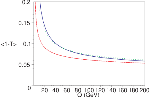
Figure 3: The average value of $\langle 1-T\rangle$ given by Eq. 49 showing the NLO prediction (dashed red), the NLO prediction with power correction of $\lambda=1$ GeV (solid blue) and an NNLO estimate with $a=3$ and a power correction of $\lambda=0.5$ GeV (green dots).

Current comparisons of NLO predictions with experimental data generally reveal the need for power corrections. For example, in electron-positron annihilation, the experimentally measured average value of 1-Thrust lies well above the NLO predictions. The difference can be accounted for by a $1/Q$ power correction. While the form of the power correction can be theoretically motivated, the magnitude is generally extracted from data and, to some extent, can be attributed to uncalculated higher orders. Including the NNLO may therefore reduce the size of the phenomenological power correction needed to fit the data.

Before the calculation of the NNLO contribution it is not possible to make a more quantitative statement. However to illustrate the qualitative point, let us take the simple example of an observable like $\langle 1-T\rangle$ which can be modelled by the simplified series,

$$\langle 1-T\rangle=0.33\alpha_{s}(Q)+1.0\alpha_{s}(Q)^{2}+a\alpha_{s}(Q)^{3}+\frac{\lambda}{Q},$$ (49)

with $\alpha_{s}(Q)\sim 6\pi/23/\log(Q/\Lambda)$ and $\Lambda=200$ MeV. Fig 3 shows the NLO perturbative prediction $a=0$, $\lambda=0$ as well as the NLO prediction combined with a power correction, $a=0$, $\lambda=1$ GeV which can be taken to model the data. If the NNLO coefficient turns out to be positive (which is by no means guaranteed), then the size of the power correction needed to describe the data will be reduced. For example, if we estimate the NNLO coefficient as $a=3$, which is large but perhaps not unreasonable, then the NLO prediction plus power correction can almost exactly be reproduced with a power correction of the same form, but $\lambda=0.6$ GeV. We are effectively trading a contribution of ${\cal O}(1/Q)$ for a contribution of $1/\log^{3}(Q/\Lambda)$. At present the data is insufficient to distinguish between these two functional forms.

2.3.2 Parton densities at NNLO

Consistent NNLO predictions for processes involving hadrons in the initial state require not only the NNLO hard scattering cross sections, but also parton distribution functions which are accurate to this order.

The evolution of parton distributions is governed at NNLO by the three-loop splitting functions, which are not fully known at present. However, using the available information on some of the lower Mellin moments [23, 24, 25] and on the asymptotic behaviour [26], as well as some exactly known terms [30], it is possible to construct approximate expressions for these splitting functions [22]. These approximations (which are provided with an error band) can serve as a substitute until full results become available [63].

The determination of NNLO parton distributions requires a global fit to the available data on a number of hard scattering observables, with all observables computed consistently at NNLO. At present, the NNLO coefficient functions are available only for the inclusive Drell-Yan process [64, 65] and for deep inelastic structure functions [66]. These two observables are by themselves insufficient to fully constrain all parton species. In the first NNLO analysis of parton distribution functions, which was performed recently [67], these processes were therefore accompanied by several other observables only known to NLO. The resulting distributions [67] illustrate some important changes in size and shape of the distribution functions in going from NLO to NNLO, visible in particular for the gluon distribution function.

It is clear that further progress on the determination of NNLO parton distributions requires a larger number of processes (in particular jet observables) to be treated consistently at NNLO.

2.3.3 Infrared limits of one-loop and tree-level processes

For simplicity let us consider a process with no initial state partons and with $m$ partons in the final state at LO. The NNLO contribution to the cross section can be decomposed as

$$\sigma^{NNLO}=\int_{m+2}d\sigma^{RR}+\int_{m+1}d\sigma^{VR}+\int_{m}d\sigma^{VV}.$$ (50)

Here $\int_{n}$ denotes the $n$-particle final state, while $d\sigma^{XY}$ denotes the fully differential cross section with double radiation ($XY=RR$), single radiation from one-loop graphs ($XY=VR$) and the double virtual contribution ($XY=VV$) that includes both the square of the one-loop graphs and the interference of tree and two-loop diagrams. After renormalisation of the virtual matrix elements, each of the contributions is UV finite. However, each of these terms is separately infrared divergent and this manifests itself as poles in $\epsilon$. Nevertheless, the Kinoshita-Lee-Nauenberg theorem states that the infrared singularities must cancel for sufficiently inclusive physical quantities. The problem is to isolate the infrared poles and analytically cancel them before taking the $\epsilon\to 0$ limit. Establishing a strategy for doing this requires a good understanding of $d\sigma^{RR}$ and $d\sigma^{VR}$ in the infrared region where the additional radiated particle(s) are unresolved.

Double unresolved limits of tree amplitudes

The infrared singular regions of tree amplitudes can be divided into several categories,

1. three collinear particles,

2. two pairs of collinear particles,

3. two soft particles,

4. one soft and two collinear particles,

5. a soft quark-antiquark pair.

In each of these limits, the tree-level $m+2$ particle amplitudes factorise and yield an infrared singular factor multiplying the tree-level $m$-particle amplitude. The various limits have been well studied.

The limit where a quark, gluon and photon simultaneously become collinear was first studied in [68] and then extended for generic QCD processes in Ref. [69] by directly taking the limit of tree-level matrix elements. These limits have been subsequently rederived using general gauge invariant methods and extended to include azimuthal correlations between the particles [70, 71, 72].

When two independent pairs of particles are collinear, the singular limits can be treated independently, and just lead to a trivial extension of the NLO result - the product of two single collinear splitting functions.

The limit where the momenta of two of the gluons simultaneously become soft has also been studied [73, 74]. At the amplitude level, the singular behaviour factorises in terms of a process independent soft two-gluon current [71] which is the generalisation of the one-gluon eikonal current.

The soft-collinear limit occurs when the momentum of one gluon becomes soft simultaneously with two other partons becoming collinear. Factorisation formulae in this limit have been provided in both the azimuthally averaged case [69] and including the angular correlations [70, 71, 72].

Finally, when the momentum of both quark and antiquark of a $q\bar{q}$ pair become soft, the tree-level amplitude again factorises [71].

Taken together, these factorisation formulae describe all of the cases where $m$-partons are resolved in a $m+2$ parton final state. Techniques for isolating the divergences have not yet been established and there is an on-going effort to develop a set of local subtraction counter-terms that can be analytically integrated over the infrared regions.

Single unresolved limits of one-loop amplitudes

The soft- and collinear-limits of one-loop QCD amplitudes has also been extensively studied. In the collinear limit, the one-loop $m+1$ particle process factorises as a one-loop $m$ particle amplitude multiplied by a tree splitting function together with a tree $m$ particle amplitude multiplied by a one-loop splitting function. The explicit forms of the splitting amplitudes were first determined to ${\cal O}(\epsilon^{0})$ [75]. However, because the integral over the infrared phase space generates additional poles, the splitting functions have been determined to all orders in $\epsilon$ [76, 77, 78, 79]. Similarly, when a gluon becomes soft, there is a factorisation of the one-loop amplitude in terms of the one-loop soft current [76, 78, 80]. Because of the similarity of the factorisation properties with the single unresolved particle limits of tree-amplitudes, it is relatively straightforward to isolate the infrared poles through the construction of a set of local subtraction counter-terms. In Sec. 2.3.5, we illustrate how the infrared singularities from the single unresolved limits of one-loop amplitudes combine with the predictable infrared pole structure of the virtual contribution for the explicit example of $\gamma^{*}\to q\bar{q}$.

2.3.4 Two-loop matrix elements for scattering processes

In recent years, considerable progress has been made on the calculation of two-loop virtual corrections to the multi-leg matrix elements relevant for jet physics, which describe either $1\to 3$ decay or $2\to 2$ scattering reactions. Much of this progress is due to a number of important technical breakthroughs related to the evaluation of the large number of different integrals appearing in the two-loop four-point amplitudes.

It should be recalled that perturbative corrections to many inclusive quantities have been computed to the two- and three-loop level already several years ago. From the technical point of view, these inclusive calculations correspond to the computation of multi-loop two-point functions, for which many elaborate calculational tools have been developed. Using dimensional regularization [81, 82, 83, 84] with $d\neq 4$ dimensions as regulator for ultraviolet and infrared divergences, the large number of different integrals appearing in multi-loop two-point functions can be reduced to a small number of so-called master integrals by using integration-by-parts identities [84, 85, 86]. These identities exploit the fact that the integral over the total derivative of any of the loop momenta vanishes in dimensional regularization.

Integration-by-parts identities can also be obtained for integrals appearing in amplitudes with more than two external legs; for these amplitudes, another class of identities exists due to Lorentz invariance of the amplitudes. These Lorentz invariance identities [87] rely on the fact that an infinitesimal Lorentz transformation commutes with the loop integral, thus relating different integrals. Using integration-by-parts and Lorentz invariance identities, all two-loop Feynman amplitudes for $2\to 2$ scattering or $1\to 3$ decay processes can be expressed as linear combinations of a small number of master integrals, which have to be computed by some different method. Explicit reduction formulae for on-shell two-loop four-point integrals were derived in [88, 89, 90]. Computer algorithms for the automatic reduction of all two-loop four-point integrals were described in [87, 91].

A related development was the proof of the equivalence of integration-by-parts identities for integrals with the same total number of external and loop momenta [92]. Consequently, much of the tools developed for the computation of three-loop propagator integrals [93, 94] can be readily applied to two-loop vertex functions. As a first application, the two-loop QCD corrections to Higgs boson production in gluon-gluon fusion were computed [95] in the limit of large top quark mass. This result allowed the complete NNLO description [96, 97, 65] of inclusive Higgs production at hadron colliders.

The master integrals relevant to $2\to 2$ scattering or $1\to 3$ decay processes are massless, scalar two-loop four-point functions with all legs on-shell or a single leg off-shell. Several techniques for the computation of those functions have been proposed in the literature, such as the application of a Mellin-Barnes transformation to all propagators [98, 99] or the negative dimension approach [100, 101]. Both techniques rely on an explicit integration over the loop momenta, with differences mainly in the representation used for the propagators. These techniques were used successfully to compute a number of master integrals. Employing the Mellin-Barnes method, the on-shell planar double box integral [98, 102], the on-shell non-planar double box integral [99] and two double box integrals with one leg off-shell [103, 104] were computed. Most recently, the same method was used to derive the on-shell planar double box integral [105] with one internal mass scale. The negative dimension approach has been applied [100] to compute the class of two-loop box integrals which correspond to a one-loop bubble insertion in one of the propagators of the one-loop box.

A method for the analytic computation of master integrals avoiding the explicit integration over the loop momenta is to derive differential equations in internal propagator masses or in external momenta for the master integral, and to solve these with appropriate boundary conditions. This method has first been suggested by Kotikov [106] to relate loop integrals with internal masses to massless loop integrals. It has been elaborated in detail and generalized to differential equations in external momenta in [107]; first applications were presented in [108, 109]. The computation of master integrals from differential equations proceeds as follows. Carrying out the derivative with respect to an external invariant on the master integral of a given topology, one obtains a linear combination of a number of more complicated integrals, which can however be reduced to the master integral itself plus simpler integrals by applying the reduction methods discussed above. As a result, one obtains an inhomogeneous linear first order differential equation in each invariant for the master integral.

The inhomogeneous term in these differential equations contains only topologies simpler than the topology under consideration, which are considered to be known if working in a bottom-up approach. The master integral is then obtained by matching the general solution of its differential equation to an appropriate boundary condition. Quite in general, finding a boundary condition is a simpler problem than evaluating the whole integral, since it depends on a smaller number of kinematical variables. In some cases, the boundary condition can even be determined from the differential equation itself.

Using the differential equation technique, one of the on-shell planar double box integrals [110] as well as the full set of planar and non-planar off-shell double box integrals [111, 112] were derived.

A strong check on all these computations of master integrals is given by the completely numerical calucations of [113], which are based on an iterated sector decomposition to isolate the infrared pole structure. The methods of [113] were applied to confirm all of the above-mentioned calculations.

The two-loop four-point functions with all legs on-shell can be expressed in terms of Nielsen’s polylogarithms [114, 115, 116, 117]. In contrast, the closed analytic expressions for two-loop four-point functions with one leg off-shell contain two new classes of functions: harmonic polylogarithms [118, 119] and two-dimensional harmonic polylogarithms (2dHPL’s) [120]. Accurate numerical implementations for these functions [119, 120] are available.

$2\to 2$ Processes with all legs on-shell

With the explicit solutions of the integration-by-parts and Lorentz-invariance identities for on-shell two-loop four-point functions [88, 89, 90] and the corresponding master integrals [121, 122, 98, 99, 102, 110], all necessary ingredients for the computation of two-loop corrections to $2\to 2$ processes with all legs on-shell are now available. In fact, only half a year elapsed between the completion of the full set of master integrals [102, 110] and the calculation of the two-loop QED corrections to Bhabha-scattering [123]. Subsequently, results were obtained for the two-loop QCD corrections to all parton-parton scattering processes [124, 125, 126, 127]. For gluon-gluon scattering, the two-loop helicity amplitudes have also been derived [128, 129]. Moreover, two-loop corrections were derived to processes involving two partons and two real photons [130, 131]. Finally, light-by-light scattering in two-loop QED and QCD was considered in [132], these results were extended to supersymmetric QED in [133].

It turns out that supersymmetry can provide strong checks on the consistency of the matrix elements. Calculations in this framework do however require modifications to the dimensional reguarization scheme, which were discussed in detail in [134].

At the same order in perturbation theory as the two-loop matrix elements (which are obtained by contracting the two-loop and the tree level amplitudes), one also finds contributions from the square of the one-loop amplitude. The evaluation of these contributions uses well-known one-loop techniques and is straightforward. For parton-parton scattering, these one-loop self-interference contributions were computed in [135, 126, 136].

The results for the two-loop QED matrix element for Bhabha scattering [123] were used in [137] to extract the single logarithmic contributions to the Bhabha scattering cross section, thus improving considerably on the accuracy of earlier [138] double logarithmic results.

$2\to 2$ Processes with one off-shell leg

With the reduction algorithm [87] and full set of two-loop master integrals [111, 112] for two-loop four-point functions now available, it is possible to compute the two-loop corrections a number of $1\to 3$ decay and $2\to 2$ scattering reactions with one off-shell leg.

As a first result (and initiated during this workshop), in [139], the two-loop QCD matrix element for $e^{+}e^{-}\to 3$ jets and the corresponding one-loop self-interference matrix element were derived. The three jet production rate in electron-positron collisions and related event shape observables are in fact the most precisely measured jet observables at present [140]. They will also play an important role in future QCD studies [141] at a the proposed high energy linear $e^{+}e^{-}$ collider.

It is worthwhile to note that besides its phenomenological importance, the three-jet rate has also served as a theoretical testing ground for the development of new techniques for higher order calculations in QCD: both the subtraction [142] and the phase-space slicing [143] methods for the extraction of infrared singularities from NLO real radiation processes were developed in the context of the first three-jet calculations. The systematic formulation of phase-space slicing [144] as well as the dipole subtraction [145] method were also first demonstrated for three-jet observables, before being applied to other processes. It is very likely that similar techniques at higher orders will first be developed in the context of jet production in $e^{+}e^{-}$ annihilation, which in contrast to hadron–hadron collisions or electron–proton scattering does not pose the additional difficulty of the regularization of initial state singularities.

Processes related to $e^{+}e^{-}\to 3$ jets by crossing symmetry are $(2+1)$-jet production in deep inelastic $ep$ scattering and vector-boson-plus-jet production at hadron colliders. Crossing of the $e^{+}e^{-}\to 3$ jets two-loop matrix element to the kinematic regions relevant for these scattering processes requires the analytic continuation of 2dHPL’s outside their range of allowed arguments. This topic is currently under investigation.

2.3.5 Infrared structure for $\gamma^{*}\to 2$ jets at NNLO

As an exercise in how to combine the various next-to-next-to-leading order contributions, we consider the infrared singularity structure for $\gamma^{*}\to 2$ jets at NNLO. This is the simplest process that we can imagine at NNLO. It involves the one- and two-loop two parton amplitudes, the one-loop three parton amplitudes and the tree-level four parton amplitudes. The aim is to symbolically identify the origins of the infrared singularities of the single and double radiation graphs. Once this is achieved, it should be possible to construct local counter terms that can be subtracted numerically from the three- and four-parton matrix elements to give infrared finite contributions and analytically integrated and combined with the explicit singularity structure of the two-parton contribution.

The one- and two-loop two parton contribution

The renormalized $\gamma^{*}\to q\bar{q}$ amplitude can be written as

$$|{\cal M}_{q\bar{q}}\rangle=\sqrt{4\pi\alpha}e_{q}\left[|{\cal M}_{q\bar{q}}^{(0)}\rangle+\left(\frac{\alpha_{s}(\mu^{2})}{2\pi}\right)|{\cal M}_{q\bar{q}}^{(1)}\rangle+\left(\frac{\alpha_{s}(\mu^{2})}{2\pi}\right)^{2}|{\cal M}_{q\bar{q}}^{(2)}\rangle+{\cal O}(\alpha_{s}^{3})\right]\;,$$ (51)

where $\alpha$ denotes the electromagnetic coupling constant, $e_{q}$ the quark charge, and the $|{\cal M}_{q\bar{q}}^{(i)}\rangle$ are the $i$-loop contributions to the renormalized amplitude. They are scalars in colour space.

The squared amplitude, summed over spins, colours and quark flavours, is denoted by

$$\langle{\cal M}_{q\bar{q}}|{\cal M}_{q\bar{q}}\rangle=\sum|{\cal M}(\gamma^{*}\to q\bar{q})|^{2}={\cal A}_{q\bar{q}}\;.$$ (52)

The perturbative expansion of ${\cal A}_{q\bar{q}}$ at renormalization scale $\mu^{2}=s_{12}$ reads,

$${\cal A}_{q\bar{q}}=4\pi\alpha\sum_{q}Ne_{q}^{2}\Bigg{[}{\cal A}^{(0)}_{q\bar{q}}+\left(\frac{\alpha_{s}(\mu^{2})}{2\pi}\right){\cal A}^{(2)}_{q\bar{q}}+\left(\frac{\alpha_{s}(\mu^{2})}{2\pi}\right)^{2}{\cal A}^{(4)}_{q\bar{q}}+{\cal O}(\alpha_{s}^{3})\Bigg{]}\;,$$ (53)

where $N$ is the number of colours and where,

$${\cal A}^{(0)}_{q\bar{q}} = \langle{\cal M}_{q\bar{q}}^{(0)}|{\cal M}_{q\bar{q}}^{(0)}\rangle=4(1-\epsilon)s_{12}\;,$$ (54)

$${\cal A}^{(2)}_{q\bar{q}} = \langle{\cal M}_{q\bar{q}}^{(0)}|{\cal M}_{q\bar{q}}^{(1)}\rangle+\langle{\cal M}_{q\bar{q}}^{(1)}|{\cal M}_{q\bar{q}}^{(0)}\rangle$$

$${\cal A}^{(4)}_{q\bar{q}} = \langle{\cal M}_{q\bar{q}}^{(1)}|{\cal M}_{q\bar{q}}^{(1)}\rangle+\langle{\cal M}_{q\bar{q}}^{(0)}|{\cal M}_{q\bar{q}}^{(2)}\rangle+\langle{\cal M}_{q\bar{q}}^{(2)}|{\cal M}_{q\bar{q}}^{(0)}\rangle\;,$$ (55)

with [146, 147, 148],

$$\langle{\cal M}_{q\bar{q}}^{(0)}|{\cal M}_{q\bar{q}}^{(0)}\rangle \equiv \includegraphics[width=71.13188pt]{m200.ps},$$ (56)

$$\langle{\cal M}_{q\bar{q}}^{(0)}|{\cal M}_{q\bar{q}}^{(1)}\rangle \equiv$$ (57)

$$= \includegraphics[width=71.13188pt]{m200.ps}\Bigg{\{}\frac{1}{2}\,C_{F}\Bigg{[}-\frac{2}{\epsilon^{2}}-\frac{3}{\epsilon}+\left(\frac{7\pi^{2}}{6}-8\right)$$

$$\hskip 99.58464pt+\left(-16+\frac{7\pi^{2}}{4}+\frac{14}{3}\zeta_{3}\right)\,\epsilon$$

$$\hskip 99.58464pt+\left(-32+\frac{14\pi^{2}}{3}+7\zeta_{3}-\frac{73\pi^{4}}{720}\right)\,\epsilon^{2}+{\cal O}(\epsilon^{3})\Bigg{]}\Bigg{\}},$$

$$\langle{\cal M}_{q\bar{q}}^{(1)}|{\cal M}_{q\bar{q}}^{(1)}\rangle \equiv$$ (58)

$$= \includegraphics[width=71.13188pt]{m200.ps}\Bigg{\{}C_{F}^{2}\Bigg{[}\frac{1}{\epsilon^{4}}+\frac{3}{\epsilon^{3}}+\left(\frac{41}{4}-\frac{\pi^{2}}{6}\right)\frac{1}{\epsilon^{2}}+\left(28-\frac{\pi^{2}}{2}-\frac{14}{3}\zeta_{3}\right)\frac{1}{\epsilon}$$

$$\hskip 99.58464pt+\left(72-\frac{41\pi^{2}}{24}-\frac{7\pi^{4}}{120}-14\zeta_{3}\right)+{\cal O}(\epsilon)\Bigg{]}\Bigg{\}},$$

$$\langle{\cal M}_{q\bar{q}}^{(0)}|{\cal M}_{q\bar{q}}^{(2)}\rangle \equiv$$ (59)

$$= \includegraphics[width=71.13188pt]{m200.ps}\Bigg{\{}\frac{1}{2\epsilon^{4}}\,C_{F}^{2}+\frac{1}{\epsilon^{3}}\left[\frac{3}{2}\,C_{F}^{2}+\frac{11}{8}C_{F}C_{A}-\frac{1}{2}C_{F}T_{R}N_{F}\right]$$

$$\hskip 85.35826pt+\frac{1}{\epsilon^{2}}\left[\left(\frac{41}{8}-\frac{13\pi^{2}}{12}\right)C_{F}^{2}+\left(\frac{4}{9}+\frac{\pi^{2}}{24}\right)C_{F}C_{A}-\frac{2}{9}C_{F}T_{R}N_{F}\right]$$

$$\hskip 85.35826pt+\frac{1}{\epsilon}\Bigg{[}\left(\frac{221}{16}-3\pi^{2}-\frac{16}{3}\zeta_{3}\right)C_{F}^{2}+\left(\frac{65}{108}+\frac{\pi^{2}}{12}\right)C_{F}T_{R}N_{F}$$

$$\hskip 99.58464pt+\left(-\frac{961}{432}-\frac{11\pi^{2}}{48}+\frac{13}{4}\zeta_{3}\right)C_{F}C_{A}\Bigg{]}$$

$$\hskip 85.35826pt+\Bigg{[}\left(\frac{1151}{32}-\frac{475\pi^{2}}{48}-\frac{29}{2}\zeta_{3}+\frac{59\pi^{4}}{144}\right)C_{F}^{2}$$

$$\hskip 99.58464pt+\left(-\frac{51157}{2592}+\frac{1061\pi^{2}}{432}+\frac{313}{36}\zeta_{3}-\frac{\pi^{4}}{45}\right)C_{F}C_{A}$$

$$\hskip 99.58464pt+\left(\frac{4085}{648}-\frac{91\pi^{2}}{108}+\frac{1}{9}\zeta_{3}\right)C_{F}T_{R}N_{F}\Bigg{]}+{\cal O}(\epsilon)\Bigg{\}}.$$

We see that the NLO part ${\cal A}^{(2)}_{q\bar{q}}$ is proportional to $C_{\scriptscriptstyle F}$ while the NNLO contribution ${\cal A}^{(4)}_{q\bar{q}}$ contains $C_{\scriptscriptstyle F}^{2}$, $C_{\scriptscriptstyle F}C_{\scriptscriptstyle A}$ and $C_{\scriptscriptstyle F}T_{R}N_{\scriptscriptstyle F}$ parts.

Catani [149] has shown how to organize the infrared pole structure of the one- and two-loop contributions renormalized in the $\overline{{\rm MS}}$ scheme in terms of the tree and renormalized one-loop amplitudes, $|{{\cal M}_{q\bar{q}}^{(0)}}\rangle$ and $|{{\cal M}_{q\bar{q}}^{(1)}}\rangle$ respectively by introducing two infrared operators, ${\mbox{\boldmath$I$}^{(1)}(\epsilon)}$ and ${\mbox{\boldmath$H$}^{(2)}(\epsilon)}$.

The form of ${\mbox{\boldmath$I$}^{(1)}(\epsilon)}$ can be simply understood by considering the total cross section to ${\cal O}(\alpha_{s})$ which is finite,

$$\includegraphics[width=71.13188pt]{m210.ps}+\includegraphics[width=71.13188pt]{m201.ps}+\includegraphics[width=71.13188pt]{m300.ps}={\rm finite}.$$ (60)

Taking soft and collinear limits of the real radiation graphs, and integrating over the unresolved phase space, we see that,

$$\longrightarrow \includegraphics[width=71.13188pt]{m200I1a.ps}+\includegraphics[width=71.13188pt]{m200I1b.ps}+{\rm finite}$$ (61)

$$= -2{\mbox{\boldmath$I$}^{(1)}(\epsilon)}\includegraphics[width=71.13188pt]{m200.ps}+{\rm finite}.$$

The symbol represents the taking of the infrared limit and integrating over the infrared phase space. This operation can be carried out in many ways. The most commonly used procedures are the subtraction formalism [142], phase space slicing method [143], as well as systematic procedures [144] and improved formulations of these methods, such as the dipole subtraction formalism [145].

In general, ${\mbox{\boldmath$I$}^{(1)}(\epsilon)}$ contains colour correlations. However, for this particular process, there is only one colour structure present at tree level which is simply $\delta_{ij}$. Adding higher loops does not introduce additional colour structures into the amplitude, and ${\mbox{\boldmath$I$}^{(1)}(\epsilon)}$ is therefore a $1\times 1$ matrix in colour space. It is proportional to $C_{\scriptscriptstyle F}$ and is given by

$${\mbox{\boldmath$I$}^{(1)}(\epsilon)}=-\frac{e^{\epsilon\gamma}}{2\Gamma(1-\epsilon)}C_{\scriptscriptstyle F}\left(\frac{2}{\epsilon^{2}}+\frac{3}{\epsilon}\right)\left(-\frac{\mu^{2}}{s_{12}+i0}\right)^{\epsilon},$$ (62)

with $\mu^{2}=s_{12}$. The double pole is due to the soft gluon singularity while the single pole is derived from the collinear quark-gluon splitting function. Inserting Eq. (61) into Eq. (60) yields the infrared singular behaviour of the one-loop amplitude,

$$\includegraphics[width=71.13188pt]{m210.ps}={\mbox{\boldmath$I$}^{(1)}(\epsilon)}\includegraphics[width=71.13188pt]{m200.ps}+{\rm finite}.$$ (63)

According to Catani [149], the infrared behaviour of the square of the one-loop contribution is given by,

$$\includegraphics[width=71.13188pt]{m211.ps}=2\Re\Biggl{[}-\frac{1}{2}\left|{\mbox{\boldmath$I$}^{(1)}(\epsilon)}\right|^{2}\includegraphics[width=71.13188pt]{m200.ps}+{\mbox{\boldmath$I$}^{(1)}(\epsilon)}\includegraphics[width=71.13188pt]{m201.ps}\Biggr{]}+{\rm finite},$$ (64)

where ${\mbox{\boldmath$I$}^{(1)}(\epsilon)}^{\dagger}$ is obtained from Eq. (62) by reversing the sign of $+i0$. The two-loop contribution can be decomposed as,

$$\includegraphics[width=71.13188pt]{m220.ps}+\includegraphics[width=71.13188pt]{m202.ps}$$ (65)

$$= 2\Re\Biggl{[}-\frac{1}{2}\left({\mbox{\boldmath$I$}^{(1)}(\epsilon)}\right)^{2}\includegraphics[width=71.13188pt]{m200.ps}+{\mbox{\boldmath$I$}^{(1)}(\epsilon)}\includegraphics[width=71.13188pt]{m210.ps}$$

$$-\frac{\beta_{0}}{\epsilon}{\mbox{\boldmath$I$}^{(1)}(\epsilon)}\includegraphics[width=71.13188pt]{m200.ps}+e^{-\epsilon\gamma}\frac{\Gamma(1-2\epsilon)}{\Gamma(1-\epsilon)}\left(\frac{\beta_{0}}{\epsilon}+K\right){\mbox{\boldmath$I$}^{(1)}(2\epsilon)}\includegraphics[width=71.13188pt]{m200.ps}$$

$$+{\mbox{\boldmath$H$}^{(2)}(\epsilon)}\includegraphics[width=71.13188pt]{m200.ps}\Biggr{]}+{\rm finite},$$

with

$$\beta_{0}=\frac{11C_{\scriptscriptstyle A}-4T_{R}N_{\scriptscriptstyle F}}{6},\qquad K=\left(\frac{67}{18}-\frac{\pi^{2}}{6}\right)C_{\scriptscriptstyle A}-\frac{10}{9}T_{R}N_{\scriptscriptstyle F}.$$ (66)

We note that the first line of the RHS of Eq. (65) is proportional to $C_{\scriptscriptstyle F}^{2}$ and produces fourth order poles in $\epsilon$, while the second line contains terms like $C_{\scriptscriptstyle F}C_{\scriptscriptstyle A}$ and $C_{\scriptscriptstyle F}T_{\scriptscriptstyle R}N_{\scriptscriptstyle F}$ and generates third order poles in $\epsilon$. The last term of Eq. (65) involving ${\mbox{\boldmath$H$}^{(2)}(\epsilon)}$ produces only a single pole in $\epsilon$ and is given by

$$\langle{{\cal M}^{(0)}}|{\mbox{\boldmath$H$}^{(2)}(\epsilon)}|{{\cal M}^{(0)}}\rangle=\frac{e^{\epsilon\gamma}}{4\,\epsilon\,\Gamma(1-\epsilon)}H^{(2)}\langle{\cal M}^{(0)}|{\cal M}^{(0)}\rangle\;,$$ (67)

where the constant $H^{(2)}$ is renormalization-scheme-dependent. As with the single pole parts of ${\mbox{\boldmath$I$}^{(1)}(\epsilon)}$, the process-dependent $H^{(2)}$ can be constructed by counting the number of radiating partons present in the event. In our case, there is only a quark–antiquark pair present in the final state, so that

$$H^{(2)}=2H^{(2)}_{q},$$ (68)

where in the $\overline{{\rm MS}}$ scheme

$$H^{(2)}_{q}=C_{F}^{2}\left(-\frac{3}{8}-6\zeta_{3}+\frac{\pi^{2}}{2}\right)+C_{F}C_{A}\left(\frac{245}{216}+\frac{13}{2}\zeta_{3}-\frac{23\pi^{2}}{48}\right)+C_{F}T_{R}N_{F}\left(-\frac{25}{54}+\frac{\pi^{2}}{12}\right)\;.$$ (69)

The singularities present in Eqs. (64) and (65) must be cancelled against the infrared poles present in the one-loop three parton and tree-level four parton contributions.

The one-loop three parton contributions

The renormalized $\gamma^{*}\to q\bar{q}g$ amplitude can be written as

$$|{\cal M}_{q\bar{q}g}\rangle=\sqrt{4\pi\alpha}e_{q}\sqrt{\left(\frac{\alpha_{s}(\mu^{2})}{2\pi}\right)}\left[|{\cal M}_{q\bar{q}g}^{(0)}\rangle+\left(\frac{\alpha_{s}(\mu^{2})}{2\pi}\right)|{\cal M}_{q\bar{q}g}^{(1)}\rangle+{\cal O}(\alpha_{s}^{2})\right]\;,$$ (70)

where the $|{\cal M}_{q\bar{q}g}^{(i)}\rangle$ are the $i$-loop contributions to the renormalized amplitude.

The squared three-parton amplitude, summed over spins, colours and quark flavours, is denoted by

$$\langle{\cal M}_{q\bar{q}g}|{\cal M}_{q\bar{q}g}\rangle=\sum|{\cal M}(\gamma^{*}\to q\bar{q}g)|^{2}={\cal A}_{q\bar{q}g}\;.$$ (71)

The perturbative expansion of ${\cal A}_{q\bar{q}g}$ at renormalization scale $\mu^{2}=s_{12}$ reads,

$${\cal A}_{q\bar{q}g}=4\pi\alpha\sum_{q}Ne_{q}^{2}\Bigg{[}+\left(\frac{\alpha_{s}(\mu^{2})}{2\pi}\right){\cal A}^{(2)}_{q\bar{q}g}+\left(\frac{\alpha_{s}(\mu^{2})}{2\pi}\right)^{2}{\cal A}^{(4)}_{q\bar{q}g}+{\cal O}(\alpha_{s}^{3})\Bigg{]}\;,$$ (72)

where,

$${\cal A}^{(2)}_{q\bar{q}g} = \langle{\cal M}_{q\bar{q}g}^{(0)}|{\cal M}_{q\bar{q}g}^{(0)}\rangle=\includegraphics[width=71.13188pt]{m300.ps},$$ (73)

$${\cal A}^{(4)}_{q\bar{q}g} = \langle{\cal M}_{q\bar{q}g}^{(0)}|{\cal M}_{q\bar{q}g}^{(1)}\rangle+\langle{\cal M}_{q\bar{q}g}^{(1)}|{\cal M}_{q\bar{q}g}^{(0)}\rangle$$ (74)

$$= \includegraphics[width=71.13188pt]{m310.ps}+\includegraphics[width=71.13188pt]{m301.ps}-\frac{\beta_{0}}{\epsilon}\includegraphics[width=71.13188pt]{m300.ps}$$

${\cal A}^{(2)}_{q\bar{q}g}$ is proportional to $C_{\scriptscriptstyle F}$, while ${\cal A}^{(4)}_{q\bar{q}g}$ contains $C_{\scriptscriptstyle F}^{2}$, $C_{\scriptscriptstyle F}C_{\scriptscriptstyle A}$ and $C_{\scriptscriptstyle F}T_{R}N_{F}$ terms [142, 143].

The virtual unresolved contributions to two-jet final states at this order arise from the one-loop corrections to $\gamma^{*}\to q\bar{q}g$ in the limit where the gluon becomes either collinear or soft. In both these limits, one observes a factorization of the renormalized matrix element. In the collinear limit, the one-loop $n+1$ parton amplitude factorises as a one-loop $n$ parton amplitude multiplied by a tree-level splitting function plus a tree-level $n$ parton amplitude multiplied by a one-loop splitting function [75, 76, 77, 78, 79]. In the soft limit, one observes the factorization of the one-loop $n+1$ parton amplitude into the one-loop $n$ parton amplitude times the leading order soft factor, plus the $n$ parton tree level amplitude multiplied with the soft gluon factor at the one-loop level [76, 78, 80]. This one-loop correction to the soft gluon factor contains only the colour factor $C_{\scriptscriptstyle A}$. In the infrared limit, we therefore obtain the usual ${\mbox{\boldmath$I$}^{(1)}(\epsilon)}$ factor multiplying the one-loop two-parton amplitude plus a new contribution ${\mbox{\boldmath$\Delta I$}^{(1)}(\epsilon)}$ multiplying the tree-level contribution,

$$\longrightarrow \includegraphics[width=71.13188pt]{m210I1a.ps}+\includegraphics[width=71.13188pt]{m210I1b.ps}$$ (75)

$$+ \includegraphics[width=71.13188pt]{m200dI1a.ps}+\includegraphics[width=71.13188pt]{m200dI1b.ps}+{\rm finite}.$$

The first term is proportional to $C_{\scriptscriptstyle F}^{2}$, while ${\mbox{\boldmath$\Delta I$}^{(1)}(\epsilon)}$ contains terms proportional to $C_{\scriptscriptstyle F}$ multiplied by double poles in $\epsilon$ and terms proportional to $C_{\scriptscriptstyle A}$. Altogether, the infrared structure from the one-loop three parton contribution is given by,

$$\includegraphics[width=71.13188pt]{m310.ps}+\includegraphics[width=71.13188pt]{m301.ps}-\frac{\beta_{0}}{\epsilon}\includegraphics[width=71.13188pt]{m300.ps}$$ (76)

$$= 2\Re\Biggl{[}-2{\mbox{\boldmath$I$}^{(1)}(\epsilon)}\includegraphics[width=71.13188pt]{m210.ps}-2{\mbox{\boldmath$\Delta I$}^{(1)}(\epsilon)}\includegraphics[width=71.13188pt]{m200.ps}$$

$$+\frac{\beta_{0}}{\epsilon}{\mbox{\boldmath$I$}^{(1)}(\epsilon)}\includegraphics[width=71.13188pt]{m200.ps}\Biggr{]}+{\rm finite}.$$

When Eq. (76) is taken together with Eqs. (64) and (65) we see that the terms of the type

$${\mbox{\boldmath$I$}^{(1)}(\epsilon)}\includegraphics[width=71.13188pt]{m210.ps}$$

and

$$\frac{\beta_{0}}{\epsilon}{\mbox{\boldmath$I$}^{(1)}(\epsilon)}\includegraphics[width=71.13188pt]{m200.ps}$$

precisely cancel.

The tree-level four parton contributions

The renormalized $\gamma^{*}\to q\bar{q}+2$ parton amplitudes can be written as

$$|{\cal M}_{q\bar{q}gg}\rangle = \sqrt{4\pi\alpha}e_{q}\left(\frac{\alpha_{s}(\mu^{2})}{2\pi}\right)\left[|{\cal M}_{q\bar{q}gg}^{(0)}\rangle+{\cal O}(\alpha_{s}^{2})\right],$$

$$|{\cal M}_{q\bar{q}q\bar{q}}\rangle = \sqrt{4\pi\alpha}e_{q}\left(\frac{\alpha_{s}(\mu^{2})}{2\pi}\right)\left[|{\cal M}_{q\bar{q}q\bar{q}}^{(0)}\rangle+{\cal O}(\alpha_{s}^{2})\right],$$ (77)

where the $|{\cal M}_{q\bar{q}pp}^{(i)}\rangle$ are the $i$-loop contributions to the renormalized amplitude for $p=g,~{}q$.

The squared four-parton amplitudes, summed over spins, colours and quark flavours, are denoted by ${\cal M}_{q\bar{q}gg}$ and ${\cal M}_{q\bar{q}q\bar{q}}$, which have the perturbative expansions,

$${\cal A}_{q\bar{q}pp}=4\pi\alpha\sum_{q}Ne_{q}^{2}\Bigg{[}\left(\frac{\alpha_{s}(\mu^{2})}{2\pi}\right)^{2}{\cal A}_{q\bar{q}pp}^{(4)}+{\cal O}(\alpha_{s}^{3})\Bigg{]}\;,$$ (78)

where,

$${\cal A}^{(4)}_{q\bar{q}gg} = \langle{\cal M}_{q\bar{q}gg}^{(0)}|{\cal M}_{q\bar{q}gg}^{(0)}\rangle=\includegraphics[width=71.13188pt]{m400gg.ps},$$ (79)

$${\cal A}^{(4)}_{q\bar{q}q\bar{q}} = \langle{\cal M}_{q\bar{q}q\bar{q}}^{(0)}|{\cal M}_{q\bar{q}q\bar{q}}^{(0)}\rangle=\includegraphics[width=71.13188pt]{m400qq.ps}.$$ (80)

The infrared singularity structure of these matrix elements is well documented in the double soft, triple collinear and independent double collinear limits [68, 69, 70, 71, 72]. At present, it is not clear how to efficiently isolate these singularities. Up to now, the only calculation involving these elements was carried out for the case of photon-plus-one-jet final states in electron–positron annihilation [68, 150], which was performed in the hybrid subtraction method, which is an extension of the phase space slicing procedure of [144]. These double unresolved factors have also been used to compute the general form of logarithmically-enhanced contributions (up to next-to-next-to-leading logarithmic accuracy) of the transverse momentum distributions of high-mass systems in hadronic collisions [151, 152].

Summary

The infrared singular structure of the two-loop amplitudes is well documented. Concerning the singular structure of the one-loop three parton amplitudes, it seems straightforward to evaluate and to construct counter terms. There is a precise cancellation with some of the singular terms in the one- and two-loop two parton contributions. However, more work is required to disentangle the singular structure of the tree-level four-parton contributions.

2.4 The high energy limit of qcd at two loops

In this section we give a summary of the present status of the analytic structure of QCD amplitudes in the limit of forward and backward scattering. The gluon and quark Regge trajectories are evaluated at two loop accuracy.

2.4.1 Forward Scattering

The scattering of two particles, with momenta $p_{1}p_{2}\to p_{3}p_{4}$ in their centre-of-mass frame, is parametrised by the invariants $s=(p_{1}+p_{2})^{2}$, $t=(p_{2}-p_{3})^{2}$ and $u=(p_{2}-p_{4})^{2}$. Since $t=-s(1-\cos\theta)/2$, where $\theta$ is the scattering angle, the kinematic region where the squared centre-of-mass energy is much greater than the momentum transfer, $s\gg|t|$, defines the forward scattering. It has been known for a long time that in the $s\gg|t|$ limit the scattering amplitudes of a gauge theory take a simple analytic form. In fact, in that limit a generic scattering process is dominated by the exchange of the particle of highest spin in the $t$ channel. That is a gluon in QCD (which we take as representative of $SU(N)$ Yang-Mills theories), a photon in QED, and a graviton in quantum gravity.

In the scattering of two partons in QCD in the limit $s\gg|t|$, the processes which yield the largest contribution are quark-quark, quark-gluon and gluon-gluon scattering. The other processes, like $q\ \bar{q}\to g\ g$, which do not feature gluon exchange in the $t$ channel, are subleading in this limit. The leading processes all have the same analytic form. In fact, the tree amplitude for parton-parton scattering $i_{a}(p_{2})\,j_{b}(p_{1})\to i_{a^{\prime}}(p_{3})\,j_{b^{\prime}}(p_{4})$, with $i,j$ either a quark or a gluon, may be written as [153]

$${\cal M}^{(0)aa^{\prime}bb^{\prime}}_{ij\to ij}=2s\left[g_{\scriptscriptstyle S}\,(T^{c}_{r})_{aa^{\prime}}\,C^{i(0)}(p_{2},p_{3})\right]{1\over t}\left[g_{\scriptscriptstyle S}\,(T^{c}_{r})_{bb^{\prime}}\,C^{j(0)}(p_{1},p_{4})\right]\,,$$ (81)

where $a,a^{\prime},b,b^{\prime}$ label the parton colours, and $r$ represents either the fundamental $(F)$ or the adjoint $(G)$ representations of $SU(N)$, with $(T^{c}_{G})_{ab}=if^{acb}$ and ${\rm tr}(T^{c}_{F}T^{d}_{F})=\delta^{cd}/2$. The coefficient function $C^{i(0)}$ is process dependent; in helicity space it just contributes a phase factor [154, 72]: its square is 1. By removing the colour factor and replacing the strong with the electromagnetic coupling, Eq. (81) holds also for the forward scattering of two charged leptons in QED with exchange of a photon in the $t$ channel.

The amplitude (81) constitutes the leading term of the BFKL theory [153, 155, 156], which models strong-interaction processes with two large and disparate scales, by resumming the radiative corrections to parton-parton scattering. This is achieved to leading logarithmic (LL) accuracy, in $\ln(s/|t|)$, through the BFKL equation, i.e. an integral equation obtained by computing the one-loop LL corrections to the gluon exchange in the $t$ channel. These corrections are: the emission of a gluon along the ladder [157], and the one-loop gluon Regge trajectory (see Eq. (88)). To see how the latter comes about, we generalise Eq. (81) to include the virtual radiative corrections and write the high-energy amplitude for parton-parton scattering, with exchange of a colour octet in the $t$ channel, as [158, 159]

$${\cal M}^{aa^{\prime}bb^{\prime}}_{ij\to ij}$$ (82)

$$= s\left[g_{\scriptscriptstyle S}\,(T^{c}_{r_{A}})_{aa^{\prime}}\,C^{i}(p_{2},p_{3})\right]{1\over t}\left[\left({-s\over-t}\right)^{\alpha(t)}+\left({s\over-t}\right)^{\alpha(t)}\right]\left[g_{\scriptscriptstyle S}\,(T^{c}_{r_{A}})_{bb^{\prime}}\,C^{j}(p_{1},p_{4})\right]$$

$$+ s\left[g_{\scriptscriptstyle S}\,(T^{c}_{r_{S}})_{aa^{\prime}}\,C^{i}(p_{2},p_{3})\right]{1\over t}\left[\left({-s\over-t}\right)^{\alpha(t)}-\left({s\over-t}\right)^{\alpha(t)}\right]\left[g_{\scriptscriptstyle S}\,(T^{c}_{r_{S}})_{bb^{\prime}}\,C^{j}(p_{1},p_{4})\right]\,,$$

with

$$(T^{c}_{G_{A}})_{aa^{\prime}}=if^{aca^{\prime}}\quad(T^{c}_{G_{S}})_{aa^{\prime}}=d^{aca^{\prime}}\quad T^{c}_{F_{A}}=T^{c}_{F}\quad T^{c}_{F_{S}}=\sqrt{N_{c}^{2}-4\over N_{c}^{2}}T^{c}_{F}\,.$$ (83)

The first (second) line of Eq. (82) corresponds to the exchange of a colour octet in the $t$ channel, of negative (positive) signature under $s\leftrightarrow u$ exchange. The function $\alpha(t)$ in Eq. (82) is the gluon Regge trajectory. It has the perturbative expansion

$$\alpha(t)=\tilde{g}_{\scriptscriptstyle S}^{2}(t)\alpha^{(1)}+\tilde{g}_{\scriptscriptstyle S}^{4}(t)\alpha^{(2)}+{\cal O}(\tilde{g}_{\scriptscriptstyle S}^{6})\,,$$ (84)

while the coefficient function can be written as

$$C^{i}=C^{i(0)}(1+\tilde{g}_{\scriptscriptstyle S}^{2}(t)C^{i(1)}+\tilde{g}_{\scriptscriptstyle S}^{4}(t)C^{i(2)})+{\cal O}(\tilde{g}_{\scriptscriptstyle S}^{6})\,.$$ (85)

In Eqs. (84) and (85), we rescaled the coupling

$$\tilde{g}_{\scriptscriptstyle S}^{2}(t)=g_{\scriptscriptstyle S}^{2}\left({\mu^{2}\over-t}\right)^{\epsilon}{1\over(4\pi)^{2-\epsilon}}\,{\Gamma(1+\epsilon)\,\Gamma^{2}(1-\epsilon)\over\Gamma(1-2\epsilon)}\,,$$ (86)

and used dimensional regularisation in $d=4-2\epsilon$ dimensions. Note that in multiplying Eq. (82) by the tree amplitude, the second line of Eq. (82) contributes only to quark-quark scattering, since the colour factor $f^{ada^{\prime}}$, occurring in any tree amplitude with an external gluon, acts as an $s$-channel projector. Then we write the projection of the amplitude (82) on the tree amplitude as an expansion in $\tilde{g}_{\scriptscriptstyle S}^{2}(t)$

$${\cal M}^{aa^{\prime}bb^{\prime}}_{ij\to ij}{\cal M}^{(0)aa^{\prime}bb^{\prime}}_{ij\to ij}=|{\cal M}^{(0)aa^{\prime}bb^{\prime}}_{ij\to ij}|^{2}\left(1+\tilde{g}_{\scriptscriptstyle S}^{2}(t)\ M^{(1)aa^{\prime}bb^{\prime}}_{ij\to ij}+\tilde{g}_{\scriptscriptstyle S}^{4}(t)M^{(2)aa^{\prime}bb^{\prime}}_{ij\to ij}+{\cal O}(\tilde{g}_{\scriptscriptstyle S}^{6})\right)\,,$$ (87)

with $i,j=g,q$.

(a)

(b)

Figure 4: Schematic one-loop expansion of the factorised form for the high energy limit of the parton-parton scattering amplitude. The pairs of concentric circles represent the one-loop corrections to the coefficient function and Regge trajectory and the individual diagrams represent terms that contribute at (a) leading and (b) next-to-leading logarithmic order.

The one-loop coefficient of Eq. (87) is,

$$M^{(1)aa^{\prime}bb^{\prime}}_{ij\to ij}=\alpha^{(1)}\ln\left({s\over-t}\right)+\ C^{i(1)}+C^{j(1)}-i{\pi\over 2}\left(1+K{N_{c}^{2}-4\over N_{c}^{2}}\right)\alpha^{(1)}\,,$$ (88)

where $K=1$ for quark-quark scattering, and $K=0$ in the other cases. Schematically, this is illustrated in Fig. 4. In Eq. (88) we used the usual prescription $\ln(-s)=\ln(s)-i\pi$, for $s>0$. The one-loop gluon Regge trajectory, $\alpha^{(1)}=2C_{\scriptscriptstyle A}/\epsilon$, Fig. 4(a), is independent of the type of parton undergoing the scattering process (it is universal). Conversely, the one-loop coefficient functions, $C^{i(1)}$, Fig. 4(b), are process and IR-scheme dependent (see Ref. [160] and references therein). They can be used to construct the next-to-leading order (NLO) impact factors, to be used in conjunction with the BFKL resummation at next-to-leading-log (NLL) accuracy [28]. Note that Eq. (88) forms a system of three equations (given by gluon-gluon, quark-quark and quark-gluon scattering) and only two unknowns: the one-loop coefficients $C^{g(1)}$ and $C^{q(1)}$. Thus, we can use two equations to determine $C^{g(1)}$ and $C^{q(1)}$, and the third to show that high-energy factorisation holds to one-loop accuracy. Finally, note that in Eq. (88) the contribution of the positive signature gluon appears in the imaginary part, thus it can contribute only to a next-to-next-to-leading order (NNLO) calculation.

(a)

(b)

(c)

Figure 5: Schematic two-loop expansion of the factorised form for the high energy limit of the parton-parton scattering amplitude. The combinations of ovals and circles represent the one-loop and two-loop corrections to the coefficient function and Regge trajectory and the individual diagrams represent terms that contribute at (a) leading, (b) next-to-leading and (c) next-to-next-to-leading logarithmic order.

The two-loop coefficient of Eq. (87) is,

$$M^{(2)aa^{\prime}bb^{\prime}}_{ij\to ij} = {1\over 2}\left(\alpha^{(1)}\right)^{2}\ln^{2}\left({s\over-t}\right)$$ (89)

$$+ \left[\alpha^{(2)}+\left(C^{i(1)}+C^{j(1)}\right)\alpha^{(1)}-i{\pi\over 2}\left(1+K{N_{c}^{2}-4\over N_{c}^{2}}\right)\left(\alpha^{(1)}\right)^{2}\right]\ln\left({s\over-t}\right)$$

$$+ \left[C^{i(2)}+C^{j(2)}+C^{i(1)}\ C^{j(1)}-{\pi^{2}\over 4}\left(1+K{N_{c}^{2}-4\over N_{c}^{2}}\right)\left(\alpha^{(1)}\right)^{2}\right]$$

$$- i{\pi\over 2}\left(1+K{N_{c}^{2}-4\over N_{c}^{2}}\right)\left[\alpha^{(2)}+\left(C^{i(1)}+C^{j(1)}\right)\alpha^{(1)}\right]\,.$$

Schematically, this is illustrated in Fig. 5. The first line of Eq. (89) is just the exponentiation of the one-loop trajectory (Fig. 5(a)). The second line of Eq. (89) allows to determine $\alpha^{(2)}$, the two-loop gluon trajectory (the first diagram in Fig. 5(b)), which provides the virtual corrections to the NLL kernel of the BFKL equation. The two-loop gluon trajectory is universal, and has been computed in Ref. [161, 162, 163, 164]. Recently it was re-evaluated in a completely independent way [160], by taking the high energy limit of the two-loop amplitudes for parton-parton scattering [126, 124, 125, 127]. The (unrenormalised) two-loop gluon Regge trajectory is

$$\alpha^{(2)}=C_{\scriptscriptstyle A}\left[\beta_{0}{2\over\epsilon^{2}}+K{2\over\epsilon}+C_{\scriptscriptstyle A}\left({404\over 27}-2\zeta_{3}\right)+N_{\scriptscriptstyle F}\left(-{56\over 27}\right)\right]\,,$$ (90)

where

$$\beta_{0}={(11C_{\scriptscriptstyle A}-2N_{\scriptscriptstyle F})\over 6},\qquad\qquad K=\left({67\over 18}-{\pi^{2}\over 6}\right)C_{\scriptscriptstyle A}-{5\over 9}N_{\scriptscriptstyle F}\,.$$ (91)

Note that at two loop accuracy, the gluon trajectory vanishes in the Abelian limit, $C_{\scriptscriptstyle A}\to 0$. That is in agreement with our expectations: in the forward scattering of two charged leptons in QED, a log of the type $\ln(s/t)$ occurs for the first time at the three loop level. Thus we expect that only in $\alpha^{(3)}$ it occurs a term which is independent of $C_{\scriptscriptstyle A}$. However, note that in QED there is no analog of Eq. (82), because the photon does not reggeise [165].

The third and fourth lines of Eq. (89) are respectively the real (Fig. 5(c)) and the imaginary parts of the constant term. Note that the gluon of positive signature does not contribute to the BFKL resummation at LL and NLL accuracy. In principle, the two-loop coefficient functions $C^{i(2)}$ could be used to construct the NNLO impact factors, if the BFKL resummation held to next-to-next-to-leading-log (NNLL) accuracy. The real constant term of Eq. (89) can be used to evaluate the two-loop coefficient functions $C^{g(2)}$ and $C^{q(2)}$. Like in Eq. (88), we have three equations (given by the two-loop amplitudes for gluon-gluon, quark-quark and quark-gluon scattering [126, 124, 125, 127]) and only two unknowns. Thus we can use two equations to evaluate $C^{g(2)}$ and $C^{q(2)}$, and the third to check if high-energy factorisation holds at NNLO accuracy. In fact, it was found that factorisation is violated [160]. That, in turn, voids the evaluation of $C^{g(2)}$ and $C^{q(2)}$. The source of the violation is not clear at present. It might be due to the (yet unknown) exchange of three or more reggeised gluons in Eq. (82).

2.4.2 Backward scattering

In the scattering of two particles in their centre-of-mass frame, $u=-s(1+\cos\theta)/2$, thus the kinematic region where $s\gg|u|$ defines the backward scattering. In this limit, we consider a scattering process with matter exchange, namely quark-gluon scattering, which proceeds via the exchange of a quark in the crossed channel. In this limit, the tree amplitude for quark-gluon scattering $q_{a}(p_{2})\ g_{b}(p_{1})\to q_{a^{\prime}}(p_{3})\ g_{b^{\prime}}(p_{4})$ can be written as

$${{\cal M}}^{(0)}_{qg\to gq}=-2i\left[g_{\scriptscriptstyle S}\,(T^{b})_{a^{\prime}i}C^{(0)}_{gq}(p_{1},p_{3})\right]\sqrt{s\over-u}\left[g_{\scriptscriptstyle S}\,(T^{b^{\prime}})_{ia}\,C^{(0)}_{qg}(p_{2},p_{4})\right]\,,$$ (92)

where $a,a^{\prime}$ ($b,b^{\prime}$) label the colour of the quarks (gluons). In helicity space, the coefficient functions $C^{(0)}$ just contribute a phase factor [166].

Generalising Eq. (92) to include virtual radiative corrections, it was shown that the quark reggeises as well. In fact, in the limit $s\gg|u|$ the amplitude for quark-gluon scattering with exchange in the $u$ channel of a colour triplet, with positive signature under $s\leftrightarrow t$ exchange, is [167]

$${{\cal M}}_{qg\to gq}=-i\left[g_{\scriptscriptstyle S}\,(T^{b})_{a^{\prime}i}C_{gq}(p_{1},p_{3})\right]\sqrt{s\over-u}\left[\left({s\over-u}\right)^{\delta(u)}+\left({-s\over-u}\right)^{\delta(u)}\right]\left[g_{\scriptscriptstyle S}\,(T^{b^{\prime}})_{ia}\,C_{qg}(p_{2},p_{4})\right]\,.$$ (93)

The function $\delta(u)$ is the quark Regge trajectory. It has the perturbative expansion

$$\delta(u)=\tilde{g}_{\scriptscriptstyle S}^{2}(u)\delta^{(1)}+\tilde{g}_{\scriptscriptstyle S}^{4}(u)\delta^{(2)}+{\cal O}(\tilde{g}_{\scriptscriptstyle S}^{6})\,,$$ (94)

with $\tilde{g}_{\scriptscriptstyle S}^{2}$ given in Eq. (86). The coefficient function $C$ has the same expansion as $C^{i}$ in Eq. (85), but for replacing $\tilde{g}_{\scriptscriptstyle S}^{2}(t)$ with $\tilde{g}_{\scriptscriptstyle S}^{2}(u)$, and like in Eq. (87), we can write the interference of Eq. (93) with the tree amplitude (92) as an expansion in $\tilde{g}_{\scriptscriptstyle S}^{2}(u)$

$${\cal M}{\cal M}^{(0)*}=|{\cal M}^{(0)}|^{2}\left(1+\tilde{g}_{\scriptscriptstyle S}^{2}(u)\ M^{(1)}+\tilde{g}_{\scriptscriptstyle S}^{4}(u)M^{(2)}+{\cal O}(\tilde{g}_{\scriptscriptstyle S}^{6})\right)\,.$$ (95)

The one-loop coefficient of Eq. (95) is

$$M^{(1)}=\delta^{(1)}\ln\left({s\over-u}\right)+\ 2C^{(1)}-i{\pi\over 2}\delta^{(1)}\,.$$ (96)

The one-loop quark trajectory is $\delta^{(1)}=2C_{\scriptscriptstyle F}/\epsilon$ [167]. Note that $\delta^{(1)}$ does not vanish in the Abelian limit $C_{\scriptscriptstyle F}\to 1$. In fact, in electron-photon scattering in QED, the electron reggeises [168, 169]. The coefficient function $C^{(1)}$ can be found in Ref. [166, 170]. The two-loop coefficient of Eq. (95) is

$$M^{(2)} = {1\over 2}\left(\delta^{(1)}\right)^{2}\ln^{2}\left({s\over-u}\right)+\left[\delta^{(2)}+2C^{(1)}\delta^{(1)}-i{\pi\over 2}\left(\delta^{(1)}\right)^{2}\right]\ln\left({s\over-u}\right)$$ (97)

$$+ \left[2C^{(2)}+\left(C^{(1)}\right)^{2}-{\pi^{2}\over 4}\left(\delta^{(1)}\right)^{2}\right]-i{\pi\over 2}\left[\delta^{(2)}+2C^{(1)}\delta^{(1)}\right]\,.$$

The first term is just the exponentiation of the one-loop trajectory. Using the two-loop amplitude for quark-gluon scattering [126], the second term of Eq. (97) allows to determine $\delta^{(2)}$, the (unrenormalised) two-loop quark Regge trajectory [166]

$$\delta^{(2)}=C_{\scriptscriptstyle F}\left[\beta_{0}{2\over\epsilon^{2}}+K{2\over\epsilon}+C_{\scriptscriptstyle A}\left({404\over 27}-2\zeta_{3}\right)+N_{\scriptscriptstyle F}\left(-{56\over 27}\right)+(C_{\scriptscriptstyle F}-C_{\scriptscriptstyle A})\left(16\zeta_{3}\right)\right]\,,$$ (98)

with $\beta_{0}$ and $K$ as in Eq. (91). Note that Eq. (98) has the remarkable feature that by mapping $C_{\scriptscriptstyle F}\to C_{\scriptscriptstyle A}$, the two-loop gluon trajectory (90) is obtained. Since the forward and backward scattering are seemingly unrelated, there is presently no understanding of why that occurs.

The second line of Eq. (97) displays respectively the real and the imaginary parts of the constant term. If Eq. (93) held at NNLO, by comparing the two-loop amplitude for quark-gluon scattering [126] with the real part of the constant term of Eq. (97) one could derive the two-loop coefficient function $C^{(2)}$. However, Eq. (93) is not expected to hold at NNLO, because of possible unknown Regge cut contributions.

2.4.3 Summary

In conclusion, we have given a summary of the present status of the analytic structure of QCD amplitudes in the limit of forward and backward scattering. We have displayed the gluon and quark Regge trajectories at two loop accuracy. They are strikingly similar: the gluon Regge trajectory can be obtained from the quark trajectory by mapping $C_{\scriptscriptstyle F}\to C_{\scriptscriptstyle A}$.

2.5 CONCLUSION AND OUTLOOK

In this working group we addressed issues related to multiparticle states at NLO and precision observables at NNLO. The motivation for this is very straightforward: we need more accurate theoretical predictions in order to make a sensible comparison with experiment, either to establish the existence of new physics or to make more precise determinations of the parameters of the theory. During the course of the workshop there has been significant progress in this field. In particular, work initiated at the workshop have yielded the following identifiable results,

• The first Feynman diagrammatic calculation of a hexagon amplitude [62]. This was performed in the Yukawa model where all external legs are massless scalars attached to a massless fermion loop. This is a good model to study how the enormous cancellations in the scalar integral reductions occur without the complications of tensor structures in the numerator. The next step is to apply these methods to realistic examples including gauge bosons and a nontrivial infrared structure. However, it is reasonable to expect that the recombination of scalar integrals will work similarly, such that efficient algorithms to calculate six-point amplitudes at one loop are in reach.

• The first evaluation of two-loop four point amplitudes with one off-shell leg [139] for the case $\gamma^{*}\to q\bar{q}g$. This process is important in determining the strong coupling constant from hadronic data in electron-positron annihilation. By analytical continuation it should be possible to extend these results to describe processes in hadron-hadron collisions, $p\bar{p}\to V+{\rm jet}$, and deep inelastic scattering, $\gamma^{*}p\to(2+1)$ jets.

• The first determination of the two-loop quark Regge trajectory [166] together with confirmation of the two-loop gluon Regge trajectory [160]. These trajectories control the behaviour of the scattering amplitudes in the high energy limit - or equivalently forward or backward scattering.

While the benefits of NLO calculations are generally well appreciated, there is some debate as to the motivation for NNLO calculations. In Sec. 2.3.1 we give reasons why NNLO predictions should qualitatively improve the agreement between theory and experiment, reduced renormalisation and factorisation scale dependence, reduced phenomenological power correction, better matching between the parton-level and hadron-level jet algorithm and a better description of the transverse momentum of the final state.

The basic ingredients for computing NNLO corrections are by now either known or conceptually understood. However a method of how to combine the individually infrared singular parts in a way that allows the construction of general purpose NNLO parton level Monte Carlo programs has not been established. This is clearly the next major task and requires considerable effort. During the workshop some preparatory steps were made in this direction for the relatively simple case of $\gamma^{*}\to q\bar{q}$ and the general structure of the infrared singularities for this process is discussed in Sec. 2.3.5. We expect that by the time of the next workshop, there will be significant progress to report.

Acknowledgements

We would like to thank the organizers of “Les Houches 2001” for creating a stimulating and productive environment for the workshop. We would like to thank our many and various collaborators for many stimulating and thought provoking discussions; T.B., J.-Ph.G. and G.H. thank C. Schubert, V.D.D and E.W.N.G. thank V. Fadin and A. Bogdan and T.G. and E.W.N.G. thank L. Garland, A. Koukoutsakis and E. Remiddi.

3 QCD RESUMMATION^, 

3.1 Introduction

In our working group we investigated a variety of issues concerning the relevance of resummation for observables at TeV colliders. Resummation is a catch-all name for efforts to extend the predictive power of QCD by summing large (logarithmic) corrections to all orders in perturbation theory. In practice, the resummation formalism depends on the observable at issue, through the type of logarithm to be resummed, and the resummation methods.

A number of resummation formalisms (threshold resummation, $Q_{T}$ or recoil resummation and any renormalization-group resummation) have now matured to the point where one can employ them for precision physics. It is known how to organize the associated logarithms to all orders and to any accuracy, at least in principle. Such resummation formalisms therefore constitute a systematically improvable calculational scheme, like standard perturbation theory. It is also known how to consistently match these resummations to finite order perturbation theory. In our working group, the full next-to-next-to-leading logarithmic threshold and $Q_{T}$ resummation were performed for the inclusive Higgs production cross section and its transverse momentum respectively. Further studies addressing the value of resummation for precision physics were done for heavy quark production cross sections and fragmentation functions. The applicability of joint resummation, the combination of threshold and recoil resummation, was examined in detail for electroweak annihilation. The relation between small-$x$ resummation, the DGLAP evolution equation, and precision analysis of the deep-inelastic structure function at HERA was further explored. Detailed application of these results to TeV colliders is still to come.

Resummed cross sections are inherently ambiguous because they require a prescription to handle singularities due to very soft radiation. These ambiguities take the form of power corrections, about which there is still much to learn. Our working group has studied the characteristics of various prescriptions, and the power corrections that they imply.

Both within our working group, and in joint sessions with others, numerous fruitful discussions took place based on short presentations by participants. These presentations and discussions addressed both the topics mentioned and reported on below, as well as the issues of resummation and Monte Carlo programs (by V. Ilyin) and next-to-next-leading logarithmic threshold resummation for Drell-Yan and deep-inelastic scattering (by A. Vogt).

In general, the studies performed in the QCD resummation working group, whose reports now follow, as well as the discussions held strengthen the view that QCD resummation does, must, and will play an important part in the quantitative study of observables at TeV colliders.

3.2 Higgs boson transverse momentum at the LHC

3.2.1 Introduction

The underlying mechanism of the electroweak symmetry breaking (EWSB) is an uncovered sector of the Standard Model (SM), thus the physical remnant of the spontaneous EWSB, the Higgs boson, is the primary object of search at present and future colliders. At the CERN Large Hadron Collider (LHC), a Standard Model (like) Higgs boson can mainly be produced in 14 TeV center of mass energy proton–proton collisions by the partonic subprocess $gg$ (via heavy quark loop) $\to HX$ (see section A.1 of ref. [1]). The extraction of the signal requires the accurate prediction of its production rate, as well as the transverse momentum ($Q_{T}$) distribution of the Higgs boson and its decay products and backgrounds, since the shape of these distributions can dictate the analysis strategies for the search [171]. To reliably predict these distributions, especially in the low to medium $Q_{T}$ region where the bulk of the rate is, the effects of the multiple soft–gluon emission have to be included. This, and the need for the systematic inclusion of the higher order QCD corrections require the extension of the standard hadronic factorization theorem to the low $Q_{T}$ region. With a smooth matching to the usual factorization formalism, it is possible to obtain a sound prediction in the full $Q_{T}$ range.

3.2.2 Low $Q_{T}$ Factorization

In this section the low transverse momentum factorization formalism is summarized briefly. We consider the case of the inclusive hard-scattering process where the final-state system $F$ is produced by the collision of the two hadrons $h_{1}$ and $h_{2}$. The final state $F$ is a generic system of non-strongly interacting particles, such as one or more vector bosons $(\gamma^{*},W,Z,\dots)$, Higgs particles ($H$) and so forth.

When calculating fixed order QCD corrections to the cross section the hadronic factorization theorem is invoked. While the transverse momentum $Q_{T}$ of the produced system is of the order of its invariant mass $Q$, this calculation is reliable. But the standard factorization fails when the $Q_{T}\ll Q$, as a result of multiple soft and collinear emission of gluons from the initial state. As an indication of this problem, the ratio of the two very different scales appear in logarithmic corrections of the form $\alpha_{S}^{n}/Q_{T}^{2}\ln^{m}Q^{2}/Q_{T}^{2}$ ($1<m<2n-1$), which spoil the convergence of fixed-order calculation in the low $Q_{T}$ region. These logarithmically-enhanced terms, not absorbed by the parton distribution functions, have to be evaluated at higher perturbative orders, and possibly resummed to all orders in the QCD coupling constant $\alpha_{s}$.

To resolve the problem, the differential cross section is split into a part which contains all the contribution from the logarithmic terms (res.), and into a regular term (fin.):

$$\frac{d\sigma_{F}}{dQdQ_{T}^{2}d\phi}=\left[\frac{d\sigma_{F}}{dQdQ_{T}^{2}d\phi}\right]_{\rm res.}+\left[\frac{d\sigma_{F}}{dQdQ_{T}^{2}d\phi}\right]_{\rm fin.}\,,$$ (99)

where $\phi$ denotes the remaining independent kinematical variables of the final system. Since the second term on the right hand side in Eq.(99) does not contain potentially large logs, it can be calculated using the usual factorization. The first term has to be evaluated differently, keeping in mind that failure of the standard factorization occurs because it neglects the transverse motion of the incoming partons in the hard scattering.

In the Fourier conjugate transverse position (${\vec{b}}$) space the resummed component of the cross section [172]–[173] can be written as

$$\frac{Q^{2}\,d\sigma_{F}}{dQ^{2}dQ_{T}^{2}d\phi}=\sum_{a,b}\int dx_{1}\,dx_{2}\,db\frac{b}{2}J_{0}(bQ_{T})\;f_{a/h_{1}}\left(x_{1},\frac{b_{0}^{2}}{b^{2}}\right)f_{b/h_{2}}\left(x_{2},\frac{b_{0}^{2}}{b^{2}}\right)s\,W_{ab}^{F}(x_{1}x_{2}s;Q,b,\phi)\,.$$ (100)

Here, the resummed partonic cross section $W_{ab}^{F}$ is

$$W_{ab}^{F}(s;Q,b,\phi) =\sum_{c}\displaystyle\int dz_{1}\,dz_{2}\;C_{ca}^{F}\left(\alpha_{s}(b_{0}^{2}/b^{2}),z_{1}\right)\;C_{{\bar{c}}b}^{F}\left(\alpha_{s}(b_{0}^{2}/b^{2}),z_{2}\right)\;\delta\left(Q^{2}-z_{1}z_{2}s\right)$$ (101)

$$\cdot\,\displaystyle\frac{d\sigma_{c{\bar{c}}}^{(LO)\,F}(Q^{2},\phi)}{d\phi}\;H_{c}^{F}\left(\alpha_{s}(Q^{2}),\phi\right)\;S_{c}(Q,b)\;\;,$$

where $\sigma_{c{\bar{c}}}^{(LO)}$ is the lowest order partonic cross-section and $S_{c}(Q,b)$ the Sudakov form factor (with $c=q,g$)

$$S_{c}(Q,b)=\exp\left\{-\int_{b_{0}^{2}/b^{2}}^{Q^{2}}\frac{dq^{2}}{q^{2}}\left[A_{c}\left(\alpha_{s}(q^{2})\right)\;\ln\left(\frac{Q^{2}}{q^{2}}\right)+B_{c}\left(\alpha_{s}(q^{2})\right)\right]\right\}\,.$$ (102)

In the usual CSS approach [174], the coefficient function $H_{c}^{F}$ does not appear (i.e. $H_{c}^{F}\equiv 1$), with the consequence that both the coefficient functions $C_{ab}(\alpha_{s}(b_{0}^{2}/b^{2}),z)$ and the Sudakov form factor $S_{c}(Q,b)$ become process dependent, a certainly unpleasent feature. As discussed in Ref. [175], the inclusion of $H_{c}^{F}$ is sufficient to make the Sudakov form factor $S_{c}(Q,b)$ and the coefficient functions $C_{ab}(\alpha_{s}(b_{0}^{2}/b^{2}),z)$ process-independent. In a similar way as it happens for parton densities, which have to be defined by fixing a factorization scheme (e.g. the ${\overline{\rm MS}}$ scheme or the DIS scheme), there is an ambiguity in the factors on the right-hand side of Eq. (101), which have to be defined by choosing a ‘resummation scheme’. Note that the choice of a ‘resummation scheme’ amounts to defining $H_{c}^{F}$ (or $C_{ab}$) for a single process. Having done that, the process-dependent factor $H_{c}^{F}$ and the universal factors $S_{c}$ and $C_{ab}$ in Eq. (101) are unambiguously determined for any other process.

The resummation formula in Eq. (101) has a simple physical origin. When the final-state system $F$ is kinematically constrained to have a small transverse momentum, the emission of accompanying radiation is strongly inhibited, so that mostly soft and collinear partons (i.e. partons with low transverse momenta $Q_{T}$) can be radiated in the final state. The process-dependent factor $H_{c}^{F}(\alpha_{s}(Q^{2}))$ embodies hard contributions produced by virtual corrections at transverse-momentum scales $Q_{T}\sim Q$. The form factor $S_{c}(Q,b)$ contains real and virtual contributions due to soft (the function $A_{c}(\alpha_{s})$ in Eq. (102)) and flavour-conserving collinear (the function $B_{c}(\alpha_{s})$ in Eq. (102)) radiation at scales $Q\raisebox{-1.72218pt}{\hbox to0.0pt{$\,\sim\,$\hss}}\raisebox{1.72218pt}{$\,>\,$}Q_{T}\raisebox{-1.72218pt}{\hbox to0.0pt{$\,\sim\,$\hss}}\raisebox{1.72218pt}{$\,>\,$}1/b$. At very low momentum scales, $Q_{T}\raisebox{-1.72218pt}{\hbox to0.0pt{$\,\sim\,$\hss}}\raisebox{1.72218pt}{$\,<\,$}1/b$, only real and virtual contributions due to collinear radiation remain (the coefficient functions $C_{ab}(\alpha_{s}(b_{0}^{2}/b^{2}),z)$).

The $A_{c}$ and $B_{c}$ functions, as well as the coefficients $C_{ab}$ are free of large logarithmic corrections and safely calculable perturbatively as expansions in the strong coupling $\alpha_{s}$

$$A_{c}(\alpha_{S})=\sum_{n=1}^{\infty}\left(\frac{\alpha_{S}}{\pi}\right)^{n}A_{c}^{(n)},~{}~{}~{}B_{c}(\alpha_{S})=\sum_{n=1}^{\infty}\left(\frac{\alpha_{S}}{\pi}\right)^{n}B_{c}^{(n)},~{}~{}~{}C_{ab}^{F}(\alpha_{s},z)=\sum_{n=0}^{\infty}\left(\frac{\alpha_{S}}{\pi}\right)^{n}C^{F(n)}_{ab}(\alpha_{S},z)\,,$$ (103)

with a similar expansion for the coefficient function $H_{c}^{F}$. More detailed expression for the coefficients can be found in [176, 177, 173, 151, 152]. The coefficients of the perturbative expansions $A_{c}^{(n)}$, $B_{c}^{(n)}$ and $C_{ab}^{F(n)}(z)$ are the key of the resummation procedure since their knowledge allows to perform the resummation to a given logarithmic order: $A^{(1)}$ leads to the resummation of leading logarithmic (LL) contributions, $\{A^{(2)},B^{(1)}\}$ give the next-to-leading logarithmic (NLL) terms, $\{A^{(3)},B^{(2)},C^{(1)}\}$ give the next-to-next-to-leading logarithmic (NNLL) terms, and so forth.

In particular, the coefficient $B^{(2)}$ has been recently computed [151, 152] for both $q\bar{q}$ and $gg$ channels allowing to extend the analysis to NNLL accuracy. Even though there is no analytical result available for it, the coefficient $A_{q,g}^{(3)}$ has been extracted numerically with a very good precision in Ref. [178]. After matching the resummed and fixed order cross sections, it is expected that the normalization of the resummed cross section reproduces the fixed order total rate (at which the $A$, $B$ and $C$ functions are evaluated), since when expanded and integrated over $Q_{T}$ they deviates only in higher order terms. [179]

3.2.3 Higgs $Q_{T}$ at the LHC using the CSS formalism

The low $Q_{T}$ factorization formalism, described in the previous section, is utilized to calculate the QCD corrections to the production of Higgs bosons at the LHC. In the low $Q_{T}$ region this calculation takes into account the effects of the multiple–soft gluon emission including the Sudakov exponent $S$, and the non–perturbative contributions ${\cal F}_{a/h}$. At the next-to-leading-logarithmic order (NLL) the $A^{(1,2)}$, and $B^{(1,2)}$ coefficients are included in the Sudakov exponent. The normalization changing effect of the ${\cal O}(\alpha_{S}^{3})$ virtual corrections are also taken into account by including the coefficient ${C}_{gg}^{(1)}$, which ensures agreement with the ${\cal O}(\alpha_{S}^{3})$ total rate. At the leading-logarithmic order (LL) the coefficients $A^{(1)}$, and $B^{(1)}$ and ${C}_{gg}^{(0)}$ are included. By matching to the ${\cal O}(\alpha_{S}^{3})$ fixed order distributions a prediction is obtained for the Higgs production cross section in the full $Q_{T}$ range which is valid up to ${\cal O}(\alpha_{S}^{3})$. The expressions for the included $A$, $B$ and $C$ coefficients and further details of this calculation are given in an earlier work. [179] The analytic results are coded in the ResBos Monte Carlo event generator.

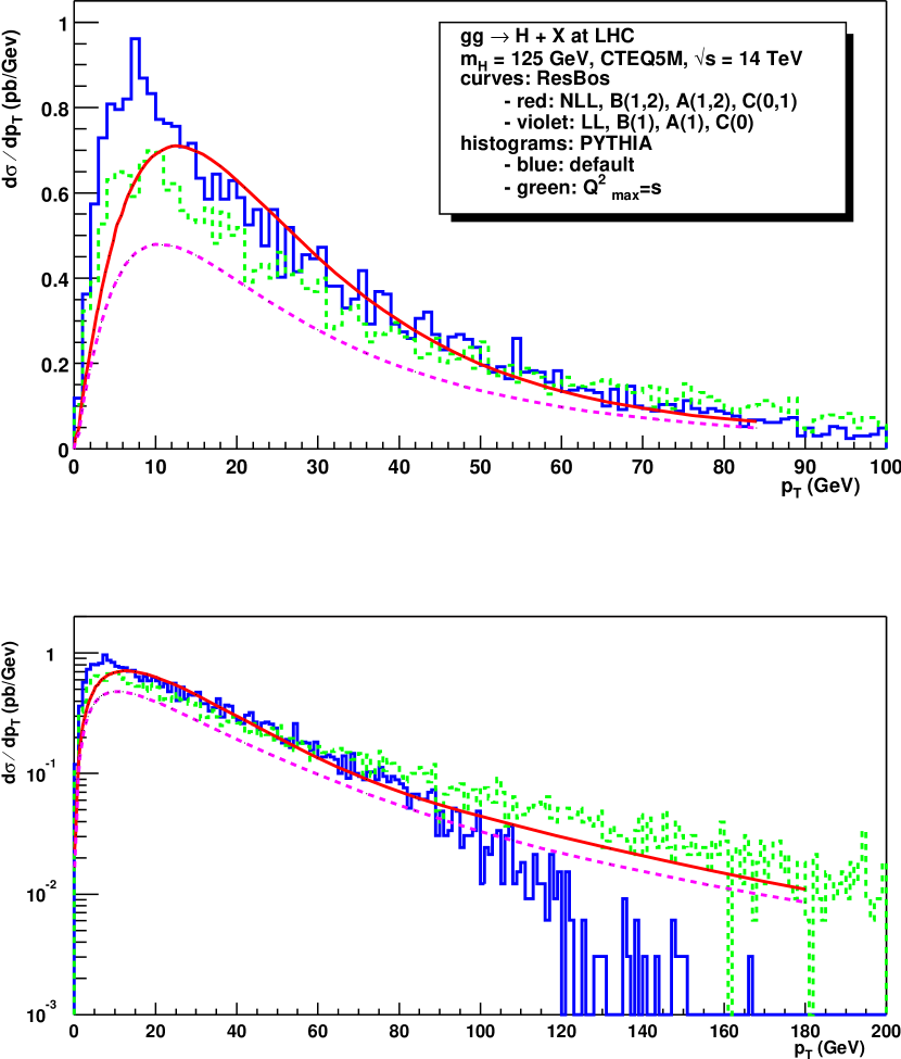
Figure 6: Higgs boson transverse momentum distributions at the LHC calculated by ResBos (curves) and PYTHIA (histograms). The solid curve was calculated at NLL (including $A^{(1,2)}$, $B^{(1,2)}$, and $C^{(0,1)}$). The dashed curve is LL (includes $A^{(1)}$, $B^{(1)}$, and $C^{(0)}$). For PYTHIA, the original output with default input parameters rescaled by a factor of $K=2$ (solid), and one calculated by the altered input parameter value $Q_{max}^{2}=s$ (dashed) are shown. The lower portion, with a logarithmic scale, also shows the high $Q_{T}$ region. In the last frame all are normalized to the solid curve.

Fig. 26 compares the Higgs boson transverse momentum distributions at the LHC calculated by ResBos (curves) and by PYTHIA (histograms from version 6.136). We use a Higgs mass of 125 GeV and CTEQ5M parton distributions. The solid curve was calculated at NLL (including $A^{(1,2)}$, $B^{(1,2)}$, and $C^{(0,1)}$). The dashed curve is LL (includes $A^{(1)}$, $B^{(1)}$, and $C^{(0)}$). The shape of these curves are quite similar reflecting the small uncertainty in the shape of the resummed prediction. The normalization changes considerably after including the sub-leading tower of logs, since both the $C^{(1)}$ and the $B^{(2)}$ coefficients receive contributions from the ${\cal O}(\alpha_{S}^{3})$ virtual corrections, which are known to be large.

In the low and intermediate $Q_{T}$ ($\lesssim 100$ GeV) region the shape of the default PYTHIA histogram agrees better with the LL ResBos curve, justifying the similar physics that goes into PYTHIA and the LL calculation. For high $Q_{T}$, the PYTHIA prediction falls under the ResBos curve, since ResBos mostly uses the exact fixed order ${\cal O}(\alpha_{S}^{3})$ matrix elements in that region, while PYTHIA still relies on the multi–parton radiation ansatz. PYTHIA can be tuned to agree with ResBos in the high $Q_{T}$ region, by changing the maximal virtuality a parton can acquire in the course of the shower (dashed histogram). Matrix element corrections to this process in PYTHIA are expected to fix this discrepancy in the near future. Since showering is attached to a process after the hard scattering takes place, and the parton shower occurs with unit probability, it does not change the total cross section for Higgs boson production given by the hard scattering rate. Thus, the total rate is given by PYTHIA at ${\cal O}(\alpha_{S}^{2})$. Thus in Fig. 26 the dashed PYTHIA histograms are plotted with their rate normalized to the NLL ResBos curve.

3.2.4 Higgs production to NNLL accuracy

As has been discussed in the introduction, the coefficients appearing in Eq. (101) (with the exception of $A^{(n)}$) are dependent on the resummation scheme. Under a change from scheme $S$ to $S^{\prime}$, the coefficients are modified as

$$H_{c\,S}^{(1)F} \to H_{c\,S^{\prime}}^{(1)F}\;,$$

$$C_{ab\,S}^{(1)}(z) \to C_{ab\,S^{\prime}}^{(1)}(z)=C_{ab\,S}^{(1)}(z)+\frac{1}{2}\delta_{ab}\delta(1-z)\left(H_{a\,S}^{(1)F}-H_{a\,S^{\prime}}^{(1)F}\right)\;,$$

$$B_{c\,S}^{(2)} \to B_{c\,S^{\prime}}^{(2)}=B_{c\,S}^{(2)}+\beta_{0}\left(H_{c\,S}^{(1)F}-H_{c\,S^{\prime}}^{(1)F}\right)$$ (104)

One possible scheme is the scheme-$H$[175], where $H_{g\,H}\equiv 1$ and the coefficients agree with the corresponding to the CSS formulation for this process. Another posibility consist in the $\overline{MS}$ scheme, where $B^{(2)}$ is defined to be proportional to the coefficient of the $\delta(1-z)$ term in the two-loop $gg$ splitting function [175]. Based on the physical interpretation of the different pieces in the resummation formulae in Eq. (101), it is possible to define the ‘collinear resummation scheme’, where only terms of collinear origin (i.e. the ones originated from the $n-4$ component of the splitting functions, see [151, 152] ) remain in the coefficient function $C$.

Even though the cross section for Higgs production is a physical observable and therefore independent on the chosen scheme, the truncation of the perturbative expansion at the level of the resummed coefficients introduces an explicit dependence on the scheme. We will use this scheme dependence as a way to quantify the perturbative stability of the resummed result, estimating the size of the unaccounted higher order terms as well as of the non-perturbative contributions. It follows from (104) that the scheme dependence first enters at the NNLL level. In Fig. 7 we show preliminary results for the $Q_{T}$ distribution for Higgs production at LHC ($M_{H}=150$ GeV) at LL, NLL and NNLL, in the last case using the three schemes discussed above.

The results are obtained using the code developed in [180], adapted for the case of inclusive Higgs production in the $gg$ channel (in the limit of infinite top quark mass) and to genuine NNLL accuracy, i.e. including up to $A^{(3)}$, $B^{(2)}$, $C^{(1)}$ and $H^{(1)}$.

Matching to the perturbative result has been performed only at LO, but this will not affect our conclusions since we are mainly interested in the low $Q_{T}$ region where the resummed contribution completely dominates the cross section. The matching at ${\cal O}(\alpha_{S}^{4})$ can be performed by using the NLO calculation of [181]. Furthermore we have not included any non-perturbative contribution and the parton distributions correspond to the CTEQ5M set.

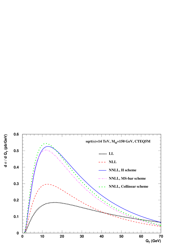
Figure 7: $Q_{T}$ distribution for Higgs production at LHC to LL, NLL and NNLL accuracy. The three NNLL lines correspond to the choice of different resummation schemes.

As can be observed, the NNLL corrections are rather large. The main reason for that is the appearence of the $C^{(1)}$ and $H^{(1)}$ coefficients, which contain the large virtual (and soft) corrections for Higgs production, which are known to considerably increase (up to almost a factor of two) the inclusive cross section. Higher order terms are expected to be smaller, at least from the observation of the rather good perturbative stability concerning the dependence on the resummation scheme at NNLL.
Acknowledgements: C.B. and D.de F. thank the organizers of the Les Houches conference for their financial support. C.B. also thanks I. Puljak for the PYTHIA curves. A.K. would like to thank W. Vogelsang for many useful discussions. D.de F. thanks M. Grazzini for discussions.

3.3 Soft-gluon effects in Higgs boson production at hadron colliders

The most important mechanism for SM Higgs boson production at hadron colliders is gluon–gluon fusion through a heavy (top) quark loop. NLO QCD corrections to this process are known to be large [182, 183, 184]: their effect increases the LO inclusive cross section by about 80-100$\%$. The NLO corrections are weakly dependent on the mass $M_{t}$ of the top quark, thus justifying the evaluation of higher-order terms within the large-$M_{t}$ approximation. Recently, the calculation of the NNLO corrections in the large-$M_{t}$ limit has been completed [95, 96, 97, 185, 65]. Their effect is moderate at the LHC: in the case of a light Higgs, the $K$-factor is about $2.3$–$2.4$, corresponding to an increase of about 25$\%$ with respect to NLO. The NNLO effect is more sizeable at the Tevatron where $K\sim 3$, the increase being of about $50\%$ with respect to NLO. The bulk of the NNLO contributions is due to soft and collinear radiation [96, 97, 185], the hard radiation [65] giving only a small (typically 5-7$\%$) correction. Multiple soft-gluon emission beyond NNLO can thus be important, particularly at the Tevatron. Here we investigate the effects of resummation of soft (Sudakov) emission to all orders. More details will be given elsewhere.

The cross section ${\hat{\sigma}}_{gg}$ for the partonic subprocess $gg\to H+X$ at the centre–of–mass energy ${\hat{s}}=M_{H}^{2}/z$ can be written as

$${\hat{\sigma}}_{gg}({\hat{s}},M_{H}^{2})=\sigma_{0}\;z\;G_{gg}(z)\;,$$ (105)

where $M_{H}$ is the Higgs mass, $\sigma_{0}$ is the Born-level cross section and $G_{gg}$ is the perturbatively computable coefficient function. Soft-gluon resummation has to be performed (see [186] and references therein) in the Mellin (or $N$-moment) space ($N$ is the moment variable conjugate to $z$). The all-order resummation formula for the coefficient function ${G}_{gg}$ is [96, 187]:

$${G}_{gg,\,N}^{{\rm(res)}}=\alpha_{s}^{2}(\mu_{R}^{2})\,C_{gg}(\alpha_{s}(\mu^{2}_{R}),M_{H}^{2}/\mu^{2}_{R};M_{H}^{2}/\mu_{F}^{2})\,\Delta_{N}^{H}(\alpha_{s}(\mu^{2}_{R}),M_{H}^{2}/\mu^{2}_{R};M_{H}^{2}/\mu_{F}^{2})\;,$$ (106)

where $\mu_{R}$ and $\mu_{F}$ denote the renormalization and factorization scales, respectively. The function $C_{gg}(\alpha_{s})$ contains all the terms that are constant in the large-$N$ limit, produced by hard virtual contributions and non-logarithmic soft corrections. It can be computed as a power series expansion in $\alpha_{s}$ as

$$C_{gg}(\alpha_{s}(\mu^{2}_{R}),M_{H}^{2}/\mu^{2}_{R};M_{H}^{2}/\mu_{F}^{2})=1+\sum_{n=1}^{+\infty}\;\left(\frac{\alpha_{s}(\mu^{2}_{R})}{\pi}\right)^{n}\;C_{gg}^{(n)}(M_{H}^{2}/\mu^{2}_{R};M_{H}^{2}/\mu_{F}^{2})\;\;,$$ (107)

where the perturbative coefficients $C_{gg}^{(n)}$ are closely related to those of the $\delta(1-z)$ contribution to $G_{gg}(z)$. The radiative factor $\Delta_{N}^{H}$ embodies the large logarithmic terms due to soft-gluon radiation. To implement resummation, the radiative factor is expanded to a given logarithmic accuracy as

$$\Delta_{N}^{H}=\exp\Big{\{}\frac{}{}\ln N\;g^{(1)}(\lambda)+g^{(2)}\!\left(\lambda,\frac{M_{H}^{2}}{\mu^{2}_{R}};\frac{M_{H}^{2}}{\mu_{F}^{2}}\right)+\alpha_{s}(\mu^{2}_{R})g^{(3)}\!\left(\lambda,\frac{M_{H}^{2}}{\mu^{2}_{R}};\frac{M_{H}^{2}}{\mu_{F}^{2}}\right)+{\cal O}(\alpha_{s}^{2}(\alpha_{s}\ln N)^{k})\Big{\}},$$ (108)

such that the functions $g^{(1)},g^{(2)}$ and $g^{(3)}$ respectively collect the leading logarithmic (LL), next-to-leading logarithmic (NLL) and next-to-next-to-leading logarithmic (NNLL) terms with respect to the expansion parameter $\lambda=\alpha_{s}(\mu^{2}_{R})\ln N$.

NLL resummation [96] is controlled by three perturbative coefficients, $A_{g}^{(1)},A_{g}^{(2)}$ and $C^{(1)}_{gg}$. The coefficients $A_{g}^{(1)}$ and $A_{g}^{(2)}$, which appear in the functions $g^{(1)}$ and $g^{(2)}$, are well known (see [186] and references therein). The coefficient $C^{(1)}_{gg}$ in Eq. (107) is extracted from the NLO result.

At NNLL accuracy three new coefficients are needed [96]: the coefficient $C_{gg}^{(2)}$ in Eq. (107) and two coefficients, $D^{(2)}$ and $A_{g}^{(3)}$, which appear in the NNLL function $g^{(3)}$. The functional form of $g^{(3)}$ was computed in Ref. [178]. The coefficients $D^{(2)}$ and $C_{gg}^{(2)}$ are obtained [96] from the NNLO result. The coefficient $A_{g}^{(3)}$ is not yet fully known: we use its exact $N_{f}^{2}$-dependence [31] and the approximate numerical estimate of Ref. [22].

Finally, to take into account the dominant collinear logarithmic terms, the coefficient $C_{gg}^{(1)}$ in the resummation formula can be modified as [96]

$$C_{gg}^{(1)}\rightarrow C_{gg}^{(1)}+2A_{g}^{(1)}\;\frac{\ln N}{N}\;.$$ (109)

In the following we present a preliminary study of the resummation effect at the Tevatron and the LHC. The hadron-level cross section is obtained by convoluting the partonic cross section in Eq. (105) with the parton distributions of the colliding hadrons. We use the MRST2000 set [188], which includes approximated NNLO parton distributions, with $\alpha_{s}$ consistently evaluated at one-loop, two-loop, three-loop order for the LO, NLO (NLL), NNLO (NNLL) results, respectively. All the results correspond to the choice $\mu_{F}=\mu_{R}=M_{H}$. The $K$-factors in Figs. 8 and 9 are defined with respect to the LO cross section. The resummed calculations are always matched to the corresponding fixed-order calculations, i.e. we consider the full fixed-order result and include higher-order resummation effects.

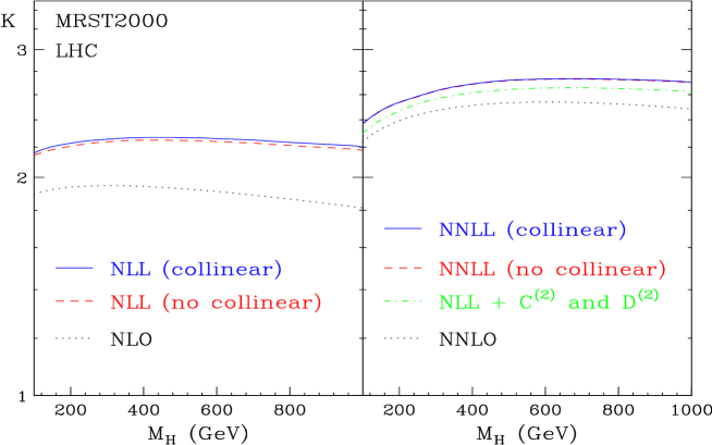
Figure 8: Resummed K-factors at the LHC.

In Fig. 8 we plot the K-factors at the LHC, as a function of the Higgs mass. On the left-hand side we show the NLL result, matched to NLO, with and without the inclusion of the collinear term in Eq. (109). The NLO result is reported for comparison. On the right-hand side we show the NNLL results, again with and without the inclusion of the collinear term. The matching is done to the NNLO result [65]. We also plot the resummed NLL result obtained by including $C_{gg}^{(2)}$ and $D^{(2)}$ only. We see that the inclusion of the collinear term is numerically not very relevant. Soft-gluon resummation at NLL accuracy increases the NLO cross section by 13-20 $\%$, the effect being more sizeable at high $M_{H}$. Going from NNLO to NNLL the effect is smaller, with an increase of $\sim 6$-9$\%$ in the full range of $M_{H}$. Note also that NLL resummation gives a good approximation of the complete NNLO calculation.

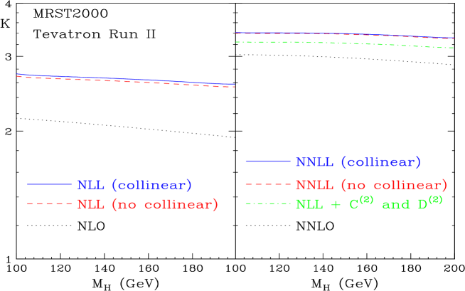
Figure 9: Resummed K-factors at the Tevatron Run II.

In Fig. 9 we report the analogous results at the Tevatron. Here the resummation effects are larger. Going from NLO to NLL accuracy, the cross section increases by 25-30$\%$. NNLL resummation increases the NNLO cross section by $\sim 12$-$16\%$ when $M_{H}$ varies in the range 100-200 GeV. These results are not unexpected [185], since at the Tevatron the Higgs boson is produced closer to threshold and the effect of multiple soft-gluon emission is more important.

3.4 Joint resummation in electroweak production

3.4.1 Introduction

The hadronic annihilation cross sections for electroweak boson production ($\gamma^{*}$, W, Z, H) provide important test cases for resummation techniques in QCD. Soft-gluon emission leads to large logarithmic contributions to perturbative cross sections, both near threshold, when the incoming partons have just enough energy to produce the observed boson, and near measured boson transverse momentum $Q_{T}\ll Q$. All-order resummations of the leading and next-to-leading terms in such contributions have been achieved separately for the threshold and small-$Q_{T}$ cases. Very recently, a formalism has been developed that encompasses both. For electroweak annihilation as well as QCD cross sections, the necessary analysis for this combination, which we refer to as joint resummation, has been carried out in [189]. In this brief report, we develop the application of the joint resummation formalism to the phenomenology of electroweak annihilation.

The effects of resummation are closely bound to momentum conservation. The singular corrections associated with soft gluon emission exponentiate in the corresponding spaces of moments, impact parameter for transverse momentum, and Mellin (or Laplace) moments in energy for threshold resummation. The transforms relax momentum and energy conservation, while their inverses reimpose it. In joint resummation, both transverse momentum and energy conservation are respected. This leads to two separate transforms in the calculation, and we will discuss below how we invert these. This is a non-trivial issue, since, taking into account nonleading logarithms and the running of the coupling, resummation leads in each case to a perturbative expression in which the scale of the coupling reflects the value of the transform variable. Because of the singularity of the perturbative effective coupling at $\Lambda_{\rm QCD}$, the resulting expressions are, strictly speaking, undefined. A closer look, however, shows that singular contributions appear only at nonleading powers of momentum transfer. This is an example of how perturbative resummation can suggest the way nonperturbative dynamics is expressed in infrared safe hard scattering functions. In effect, perturbation theory is ambiguous, and the resolution of its ambiguities is, by definition, nonperturbative [190, 191, 192]. Each scheme for dealing with these ambiguities constitutes a specification of perturbation theory, and implies a parameterization of nonperturbative effects. We hope that a joint resummation affords a more general approach to this problem.

3.4.2 Joint resummation method

In the framework of joint resummation [189], the cross section for electroweak annihilation is given as

$$\frac{d\sigma_{AB}^{\rm res}}{dQ^{2}\,dQ_{T}^{2}} = \sum_{a}\sigma_{a}^{(0)}\,\int_{C_{N}}\,\frac{dN}{2\pi i}\,\tau^{-N}\;\int\frac{d^{2}b}{(2\pi)^{2}}\,e^{i{\vec{Q}_{T}}\cdot{\vec{b}}}\,$$ (110)

$$\times {\cal C}_{a/A}(Q,b,N,\mu,\mu_{F})\;\exp\left[\,E_{a\bar{a}}^{\rm PT}(N,b,Q,\mu)\,\right]\;{\cal C}_{\bar{a}/B}(Q,b,N,\mu,\mu_{F})\;,$$

where $\tau=Q^{2}/S$, $Q$ denotes the invariant mass of produced boson, and $\sigma_{a}^{(0)}$ is the Born cross section. The flavour-diagonal Sudakov exponent $E_{a\bar{a}}^{\rm PT}$ is given to next-to-leading logarithmic (NLL) accuracy by

$$\tilde{E}_{a\bar{a}}^{\rm PT}(N,b,Q,\mu,\mu_{F}) = -\int_{Q^{2}/\chi^{2}}^{Q^{2}}\frac{dk_{T}^{2}}{k_{T}^{2}}\;\left[A_{a}(\alpha_{s}(k_{T}))\,\ln\left(\frac{Q^{2}}{k_{T}^{2}}\right)+B_{a}(\alpha_{s}(k_{T}))\right]\,.$$ (111)

It has the classic form of the Sudakov exponent in the recoil-resummed $Q_{T}$ distribution for electroweak annihilation, with the same functions $A$ and $B$. The latter are perturbative series in $\alpha_{s}$ [172, 193]; at NLL, one only needs the second (first) order expansion of $A$ ($B$) [176]. The only difference between the standard Sudakov exponent for $Q_{T}$ resummation and Eq. 111 comes from the lower limit of the integrand, i.e. the function $\chi$ that organizes the logarithms of $N$ and $b$ in joint resummation:

$$\chi(\bar{N},\bar{b})=\bar{b}+\frac{\bar{N}}{1+\eta\,\bar{b}/\bar{N}}\;\qquad\qquad\bar{b}\equiv bQ{\rm e^{\gamma_{E}}}/2\;.$$ (112)

This choice for $\chi(\bar{N},\bar{b})$ fulfills the requirement of reproducing the LL and NLL terms in $N$ and $b$ when $N\rightarrow\infty$ (at fixed $b$) and $b\rightarrow\infty$ (at fixed $N$). Moreover, it also guarantees that in the limit $b\gg N$ the quantity $E_{a\bar{a}}^{\rm PT}$ expanded up to ${\cal O}(\alpha_{s})$ does not have any subleading terms with singular behavior different from the one present in the fixed-order result.

The functions ${\cal C}(Q,b,N,\mu,\mu_{F})$ in Eq. (110)

$${\mathcal{C}}_{a/H}(Q,b,N,\mu,\mu_{F})=\sum_{j,k}C_{a/j}\left(N,\alpha_{s}(\mu)\right)\,{\cal E}_{jk}\left(N,Q/\chi,\mu_{F}\right)\,f_{k/H}(N,\mu_{F})\;,$$ (113)

contain products of parton distribution functions $f_{k/H}$ at scale $\mu_{F}$ with an evolution operator ${\cal E}_{jk}$ between scales $\mu_{F}$ and $Q/\chi$. Furthermore, as familiar from both threshold and $Q_{T}$ resummation, they contain hard coefficients $C_{a/j}(N,\alpha_{s})$ that are again perturbative series in $\alpha_{s}$ and have the first-order expansions

$$C_{q/q}^{(1)}\left(N,\alpha_{s}\right) = 1+\frac{\alpha_{s}}{4\pi}C_{F}\left(-8+\pi^{2}+\frac{2}{N(N+1)}\right)\;=\;C_{\bar{q}/\bar{q}}^{(1)}\left(N,\alpha_{s}\right)\;,$$ (114)

$$C_{q/g}^{(1)}\left(N,\alpha_{s}\right) = \frac{\alpha_{s}}{2\pi}\frac{1}{(N+1)(N+2)}\;=\;C_{\bar{q}/g}^{(1)}\left(N,\alpha_{s}\right)\;.$$ (115)

To be consistent with the NLL approximation for the $E_{a\bar{a}}^{\rm PT}$ part of the cross section, the evolution matrix ${\cal E}$ is derived from the NLO solutions of standard evolution equations [17]. Inclusion of the full evolution of parton densities (as opposed to keeping only the $\sim\ln\bar{N}$ part of the anomalous dimension that dominates near threshold, see Ref. [194]) extends the joint formalism and leads to resummation of collinear logarithms not all of which are associated with threshold corrections.

Owing to the presence of the Landau pole in the strong coupling, the jointly resummed cross section (110) requires definitions for the inverse Mellin and Fourier transforms. In pure threshold resummation, it was proposed to parameterize the inverse Mellin contour as [186]

$$N=C+z{\rm e}^{\pm i\phi}\;,$$ (116)

where $C$ lies to the right of the singularities of the parton densities, but to the left of the Landau pole. This is a natural definition of the contour since it decouples the Landau pole from any finite-order expansion of the resummed cross section. For the jointly resummed cross section in Eq. (110), if the $b$ integration is carried out in the standard way over the real axis, one will inevitably reach the Landau pole. This is well-known also from pure $Q_{T}$ resummation and led to the introduction of a (non-perturbative) upper value $b_{\rm max}$ for the $b$ integral, along with a redefinition $b\to b_{\ast}=b/\sqrt{1+b^{2}/b_{\rm max}^{2}}$. To avoid introducing a new parameter, we treat the $b$ integral in a manner analogous to the $N$ integral above [195]: were the Landau pole not present we could, instead of performing the $b$ integral along the real axis, use Cauchy’s theorem and divert it into complex $b$ space. Our prescription will be to use the diverted contour also in the presence of the Landau pole. Technically, this can be achieved by writing

$$2\pi\,\int_{0}^{\infty}\,db\,b\,\,J_{0}(bQ_{T})\,f(b)=\pi\,\int_{0}^{\infty}db\,b\,\left[\,h_{1}(bQ_{T},v)+h_{2}(bQ_{T},v)\,\right]\,f(b)\,,$$ (117)

where the $h_{i}$ are related to Hankel functions and distinguish positive and negative phases in Eq. (117). We then can treat the $b$ integral as the sum of two contours, the one associated with $h_{1}$ ($h_{2}$) corresponding to closing the contour in the upper (lower) half $b$-plane [195].

3.4.3 Transverse momentum distribution for $Z$ production

A phenomenological application of the joint resummation formalism requires matching the resummed distribution (110) to the fixed-order result $d\sigma^{\rm fixed}$, which we do as follows:

$$\frac{d\sigma}{dQ^{2}dQ_{T}^{2}}=\frac{d\sigma^{\rm res}}{dQ^{2}dQ_{T}^{2}}-\frac{d\sigma^{\rm exp(k)}}{dQ^{2}dQ_{T}^{2}}+\frac{d\sigma^{\rm fixed(k)}}{dQ^{2}dQ_{T}^{2}}\,,$$ (118)

with $d\sigma^{\rm exp(k)}$ denoting the $k$-th order expansion of the resummed cross section. This way of matching in the conjugate $(N,\,b)$ space evidently avoids any type of double counting. Given the above prescription we calculate the $Q_{T}$ distribution for Z production at the Tevatron and compare it with the latest CDF data [196] in Fig. 10 (dashed lines). We emphasize that the dashed lines are obtained without any additional nonperturbative parameter. Towards low $Q_{T}$, one expects perturbation theory (as defined in our formalism) to fail without nonperturbative input. The expected form of such effects can be derived from resummed perturbation theory itself [194, 192, 197] by examining the full NLL jointly resummed exponent in the limit of small transverse momentum of soft radiation. The gross structure one finds is a simple Gaussian function $-gb^{2}$ added to the Sudakov exponent in (110). A fit to the data gives a modest $g=0.8$ GeV², similar to [198]. We finally note that, unlike standard $Q_{T}$ resummation, our resummed cross section (118) stays positive even at very large $Q_{T}$ so that an extra switching between a matched distribution and a fixed order result is not required here. We obtain a very good agreement between data and the jointly resummed theoretical distribution even out to large $Q_{T}$.

Figure 10: CDF data [196] on Z production, compared to joint resummation predictions (matched to the ${\cal O}(\alpha_{s})$ result according to Eq. (118)) without nonperturbative smearing (dashed) and with Gaussian smearing using the nonperturbative parameter $g=0.8$ GeV² (solid). The normalizations of the curves (factor of 1.069) have been adjusted in order to give an optimal description. We use CTEQ5M parton distribution functions with renormalization and factorization scales $\mu=\mu_{F}=Q$.

3.5 Transverse momentum and threshold resummations in heavy quark production

Theoretical analysis of QCD problems involving a single scale parameter is highly developed; however, the problem becomes complex when more than one distinct scale is involved. Unfortunately, most of the interesting experimental measurements fall in the multi-scale category. In recent years, powerful theoretical tools have been developed to describe such complex reactions. The fundamental problem with the analysis of multi-scale regimes in the context of perturbation theory is that the truncated series in the strong coupling $\alpha_{s}$ may converge poorly due to the presence of large logarithms of dimensionless quantities. The “big bad logs” can appear in a number of guises. Logarithms of the form ($\alpha_{s}^{n}/q_{T}^{2})\ln^{m}(q_{T}^{2}/Q^{2})$, $m\leq 2n-1$ appear when calculating differential distributions in transverse momentum. Separately, we encounter logarithms of the form $\alpha_{s}^{n}[\ln^{m}(1-z)/1-z]_{+}$, $m\leq 2n-1$, with $z=Q^{2}/s$, in the production of heavy quarks near threshold. The solution to the problem is to find all-order sums of large logarithmic terms from first principles of the theory, such as gauge and renormalization group invariance.

The soft-gluon resummation formalism of Collins, Soper, Sterman (CSS) [199, 174] sums large logs of the form $\ln^{m}(q_{T}^{2}/Q^{2})$; this formalism has enjoyed a number of theoretical advances in recent years [200]. Logarithms of the second type, $\ln^{m}(1-z)$, arise in the production of heavy quarks near threshold [201, 202, 203, 204, 205]. More recently, new techniques have been developed to perform joint resummation to handle both types of logs simultaneously [189].

In this study, we address the impact of $q_{T}$ and threshold logarithms on the heavy quark production. Our approach is to first examine the $q_{T}$ and threshold resummation results separately, compare the contributions in various kinematic regions, and finally consider the joint resummation. The dependence of results on the mass $M$ of the heavy quarks gives an additional dimension to this problem. Our work on $q_{T}$ resummation is motivated, in part, by recently calculated ${\cal O}(\alpha_{s})$ cross sections for heavy quark production in semi-inclusive deep-inelastic scattering (SIDIS) [206], and by newly developed methods for resummation of $q_{T}$ logarithms in massless SIDIS [207, 208, 209]. These results can be combined to obtain improved description of differential heavy-quark distributions in a large range of collision energies.

Our calculations use the ACOT variable flavor number factorization scheme [210, 211], which itself is a resummation of logarithms involving the heavy quark mass via the DGLAP evolution equation. This scheme is successfully applied to obtain accurate predictions for inclusive quantities (e.g. the charm structure function $F_{2}^{c}(x,Q^{2})$) both at asymptotically high energies $s\gg M^{2}$ and near the threshold $s\approx M^{2}$.

For less inclusive observables, application of the ACOT scheme in a fixed-order calculation is often not sufficient due to the presence of logarithms different from $\ln(Q^{2}/M^{2})$. Fixed-order calculations, such as the calculation in [206], have to combine subprocesses with different numbers of final-state particles. This combination leads to unphysical “plus” and “delta-function” distributions; it also leaves large logarithmic terms in the coefficient functions. The dynamical origin of this deficiency lies in the intensive soft QCD radiation, which accompanies particle reactions near boundaries between $n$- and $(n+1)$-particle kinematics. In SIDIS, unphysical distributions appear in the current fragmentation region, which in our notations corresponds to the limit $q_{T}^{2}\ll Q^{2}$. Note that this phenomenon occurs when the hard scale of the reaction is much larger than the heavy-quark mass, i.e., $Q^{2}\gg M^{2}$.

The key result of the CSS resummation formalism is that all large logarithms due to the soft radiation in the high-energy limit can be resummed into a Sudakov exponent. This result can be summarized in the following master equation:

$$\frac{d\sigma}{dQ^{2}\,dq_{T}^{2}}=\frac{\sigma_{0}}{s}\ \int\frac{d^{2}b}{(2\pi)^{2}}\ e^{i\vec{q}_{T}\cdot\vec{b}}\ \left(C^{\mathrm{in}}\otimes f\right)\left(C^{\mathrm{out}}\otimes d\right)e^{-S}\ +\sigma_{\mathrm{FO}}-\sigma_{\mathrm{ASY}}\,.$$ (119)

Here $b$ is the impact parameter, $f$ and $d$ are parton distribution functions and fragmentation functions, respectively. $C^{\mathrm{in}}$, $C^{\mathrm{out}}$ contain perturbative corrections to contributions from the incoming and outgoing hadronic jets, respectively. The factor $e^{-S}$ is the Sudakov exponential, which includes an all-order sum of perturbative logarithms $\ln^{m}{q_{T}^{2}/Q^{2}}$ at $b\lesssim 1\mbox{ GeV}^{-1}$ and nonperturbative contributions at $b\gtrsim 1\mbox{ GeV}^{-1}$. Finally, $\sigma_{\mathrm{FO}}$ is the fixed-order expression for the considered cross section, while $\sigma_{\mathrm{ASY}}$ (asymptotic piece) is the perturbative expansion of the $b$-space integral up to the same order of $\alpha_{s}$ as in $\sigma_{FO}$. At small $q_{T}$, where terms $\ln^{m}(q_{T}^{2}/Q^{2})$ are large, $\sigma_{\mathrm{FO}}$ cancels well with $\sigma_{\mathrm{ASY}}$, so that the cross section (119) is approximated well by the $b$-space integral. At $q_{T}\gtrsim Q$, where the logarithms are no longer dominant, the $b$-space integral cancels with $\sigma_{\mathrm{ASY}}$, so that the cross section (119) is equal to $\sigma_{\mathrm{FO}}$ up to higher order corrections.

Figure 11: Balance of various terms in the ACOT scheme and resummed cross section. Graphs show $q_{T}$ on the $x$-axis and $d\sigma/dq_{T}^{2}$ on the $y$-axis.

In extending the CSS resummation from the massless to the massive case, we observe that the proof of the resummation formula in the original papers [199, 174] does not require quarks to be massless; nor does it rely on the usage of the $\overline{MS}$ scheme for regularization of soft and collinear singularities. Hence the reorganization of perturbative calculations as in Eq. (119) is also justified for massive quarks. Note, however, that nonvanishing quark masses regulate collinear singularities, so that at least some of the logarithms are not dominant in the threshold region. On the other hand, the discussion in Ref. [211] suggests that masses can be set to zero for those heavy quarks that enter the hard scattering subprocess directly from the proton.

This approximation, which differs from the complete mass-dependent cross section by higher-order terms, significantly simplifies the analysis. We therefore drop heavy-quark masses in the hard scattering subdiagrams with incoming heavy quark lines. This approximation leads to massless expressions for the perturbative Sudakov factor and $C$-functions for quark-initiated subprocesses, and mass-dependent $C$-functions for gluon-initiated subprocesses.

Figure 11 qualitatively illustrates the balance of various terms in the resummation formula in various regions of phase space for the lowest-order contributions. First, consider a fixed-order calculation in the simplified ACOT scheme near the threshold. In this region, the cross section $d\sigma/dq_{T}^{2}$ is well approximated by the ${\cal O}(\alpha_{s})$ photon-gluon diagram (Fig. 11a). To this diagram, we add the lowest-order $\gamma^{*}q$ term, which resums powers of $\ln(Q^{2}/M^{2})$ and contributes at $q_{T}=0$ (Fig. 11b). We also subtract the overlap between the two diagrams (Fig. 11c), which is approximately equal to, but not the same as, the $\gamma^{*}q$ contribution. The resulting distribution (Fig. 11d) is close to the fixed-order result, but has discontinuities in the small $q_{T}$ region. These discontinuities are amplified when $Q$ increases.

In the resummed cross section, the fusion diagram still dominates near the threshold, but now the resummed cross section and subtracted asymptotic piece are smooth functions, which cancel well at all values of $q_{T}$ (Fig. 11e-h). Hence, the distribution is physical in the whole range of $q_{T}$. Finally, at $Q^{2}\gg M^{2}$ the small-$q_{T}$ region the $\gamma^{*}g$ fusion contribution is dominated by the $1/q_{T}^{2}$ term (Fig. 11i). Such singular terms are summed through all orders in the $b$-space integral corresponding to Fig. 11j and are canceled in the fusion contribution by subtracting the asymptotic piece (Fig. 11k).

As mentioned above, threshold resummation organizes logs of the form $\alpha_{s}^{n}[\ln^{m}(1-z)/1-z]_{+}$, which can yield a large contribution when $z\rightarrow 1$ [201, 202, 203, 204, 205]. When combining the results of both the $q_{T}$ and threshold resummation, an important consideration is whether there is an overlap in resummed terms, which would result in double counting. While in a general context this delicate problem makes the double resummation non-trivial, this is not an issue for the low order case we are examining here; for this reason, we can compute the contributions separately and compare them without any complications.

Our analysis in this study will continue well past the time scale of the present workshop, and detailed results will be described in a separate publication. New experimental measurements will contain a wealth of information of high precision – if only we can extract and analyze it. Theoretical tools must be refined to keep up with this progress. The resummation formalisms that we are studying here provide an efficient way to go beyond low order perturbative calculations and describe the heavy quark data accurately in a wide range of kinematical variables. With these new methods at hand, we will be well prepared for examination of new detailed information from HERA, TEVATRON Run II, and the LHC.

3.6 Soft gluon resummation for fragmentation functions

When one is considering the issue of performing tests of perturbative QCD (pQCD) predictions and of calculational techniques, production processes involving heavy quarks (i.e. of mass $m\gg\Lambda_{QCD}$) can be thought of as an ideal choice for at least two distinct reasons.

• The large mass of the quark acts as a cutoff for collinear singularities, allowing perturbative calculations to give finite results without resorting to factorization into phenomenological functions, hence allowing, at least in principle, direct comparisons to experimental data.

• When the quarks undergo a non-perturbative hadronization before being observed, say, as a heavy-light meson like $D$ or $B$, the extent to which this process modifies the perturbative predictions can be expected to be of the order of magnitude of (powers of) the ratio $\overline{\Lambda}/m$, where $\overline{\Lambda}$ is a hadronic scale of the order of a few hundred MeV . One can therefore hope to be less dependent on the inclusion of non-perturbative parametrizations (for instance parton distribution and fragmentation function) which, by introducing additional phenomenological degrees of freedom, can obscure the real predictive power of the underlying theoretical framework.

Such nice features do of course come at a price. Perturbative calculations, while finite, will however contain in higher order logarithms of the various physical scales entering the problem. For instance, heavy quark hadroproduction at transverse momentum $p_{T}$ or heavy quark fragmentation in $e^{+}e^{-}$ collisions at a center-of-mass energy $Q$ will display $\alpha_{s}^{2}(\alpha_{s}^{n}\log^{k}(p_{T}/m))$ or $\alpha_{s}^{n}\log^{k}(Q/m)$ (with $0\leq k\leq n$) terms respectively. When $Q,\;p_{T}\gg m$ such logarithms, remnants of the screening of the collinear singularities, grow large, eventually spoiling the convergence of perturbation theory. Analogously, observing the heavy quark close to a phase space boundary will constrain soft radiation and result in Sudakov logarithms which can also grow very large.

Therefore, in order to really exploit the aforementioned possibly superior qualities of heavy quark processes, one must first take care of properly and accurately evaluating the perturbative result. In particular, this means performing an all-order resummation of the large logarithms previously mentioned, and matching to an exact fixed order result for recovering the non-leading terms.

Resummation of “collinear” large logarithms to next-to-leading log (NLL) accuracy was first performed in Ref. [212, 213] for $e^{+}e^{-}$ collisions. Sudakov logarithms were also resummed to leading logarithmic order (LL). Reference [214] extended the resummation of Sudakov logs to NLL level.

The papers previously mentioned only directly addressed heavy quark production in $e^{+}e^{-}$ collisions. Reference [212, 213] did however put forward convincing arguments about the existence of a process-independent heavy quark fragmentation function. Making use of this universality, NLL resummation of collinear logs was first performed for hadron-hadron collisions in [215], and then extended to other processes as well [216, 217]. These resummations where then matched to complete next-to-leading (NLO) perturbative calculations [218, 219] to provide reliable results in the whole range of transverse momenta.

The universality has recently been fully exploited in Ref. [220], where the heavy quark fragmentation function has been extracted by making no reference to any explicit production process. The production cross section for a heavy quark of mass $m$ at a scale $Q$ (or $p_{T}$) can therefore always be written as a convolution of this process-independent function $D^{\rm ini}(\mu_{F},m)$ and a process dependent coefficient function $C(Q,\mu_{F})$:

$$\sigma(Q,m)=C(Q,\mu_{F})\otimes D^{\rm ini}(\mu_{F},m)+{\cal O}((m/Q)^{p})\;.$$ (120)

The factorization scale $\mu_{F}$ separates the two functions, and Altarelli-Parisi evolution can be used to resum the collinear logarithms in $D^{\rm ini}(\mu_{F},m)$ by evolving from an initial scale $\mu_{0F}\simeq m$ up to the hard scale $\mu_{F}\simeq Q$, so that $D^{\rm ini}(\mu_{F},m)=E(\mu_{F},\mu_{0F})\otimes D^{\rm ini}(\mu_{0F},m)$.

Making use of this factorization it has been possible to resum the Sudakov logarithms to NLL accuracy for $D^{\rm ini}(\mu_{0F},m)$ and $C(Q,\mu_{F})$ separately. The resummed result for $D^{\rm ini}(\mu_{0F},m)$ is, of course, also process independent (though factorization-scheme dependent), and its Mellin moments can be written (we use the ${\overline{\rm MS}}$ factorization-scheme) in the form [220]:

$$D_{N}^{{\rm ini},\,S}(\alpha_{s}(\mu_{0}^{2});\mu_{0}^{2},\mu_{0F}^{2},m^{2}) \!\!\!= \!\!\!\left\{1+\frac{\alpha_{s}(\mu_{0}^{2})C_{F}}{\pi}\left[-\frac{\pi^{2}}{6}+1-\gamma_{E}^{2}+\gamma_{E}+\left(\frac{3}{4}-\gamma_{E}\right)\ln\frac{\mu_{0F}^{2}}{m^{2}}\right]\right\}$$ (121)

$$\!\!\!\times \!\!\!\exp\Bigl{[}\ln N\;g^{(1)}_{\rm ini}(\lambda_{0})+g^{(2)}_{\rm ini}(\lambda_{0},m^{2}/\mu_{0}^{2};m^{2}/\mu_{0F}^{2})\Bigr{]}\,.$$

Explicit results for the $g_{\rm ini}^{(1)}$ and $g_{\rm ini}^{(2)}$ functions can be found in Ref. [220].

Contrary to that of the “collinear” $\log(p_{T}/m)$ terms, resummation of the Sudakov logs is not of direct phenomenological importance for studying inclusive $p_{T}$ distributions in heavy quark production at the Tevatron or the LHC. Indeed, unless one gets very close to phase space limits, only low-$N$ moments of $D_{N}^{{\rm ini}}$, around $N\sim 5$, are relevant[221]. Sudakov resummation, on the other hand, starts producing visible effects around $N\sim 10$ [220].

Having a reliable theoretical prediction for $D^{{\rm ini}}(\mu_{0F},m)$ (and, with the analogous NLL Sudakov resummation of $C(Q,\mu_{F})$ also performed in Ref. [220], for the measurable single-inclusive heavy-quark cross section in $e^{+}e^{-}$ collisions) is however useful when extracting from experimental data the non-perturbative contributions which must complement the perturbative calculation in order to get a good description of the data. A generic “hadron level” cross section for $B$ or $D$ meson production in $e^{+}e^{-}$ or hadron collisions can be described by

$$\sigma_{\rm had}(Q,m)=C(Q,\mu_{F})\otimes D^{\rm ini}(\mu_{F},m)\otimes D^{\rm np}(\epsilon_{1},...,\epsilon_{n})\;.$$ (122)

The function $D^{\rm np}(\epsilon_{1},...,\epsilon_{n})$ can represent either a phenomenological parametrization or an attempt to establish the form of such a contribution through the analysis of power corrections. It can be argued [222, 223] that it will be, at least to some reasonable accuracy level, as process independent as its perturbative counterpart $D^{\rm ini}(\mu_{F},m)$. In any case, it will depend on a set of parameters $(\epsilon_{1},...,\epsilon_{n})$ which, pending a full solution of non-perturbative QCD, can only be determined by comparison with the data.

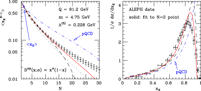
Figure 12: ALEPH data for weakly-decaying $B$ mesons are fitted to a convolution of the perturbative prediction and a non-perturbative function (see text). Solid line: $\alpha=27.45$, fitted in $N$ space, fixed by the $\langle x_{E}\rangle$ (i.e. $N=2$) point only. Dashed line: $\alpha=29.1$, fitted as before, but no Sudakov resummation in the pQCD part. Dotted line: $\alpha=17.7$, fitted with resummation and using all points in $x_{E}$ space. The dot-dashed line is the purely perturbative contribution, as defined in Ref. [220].

An example of such a determination is given in Fig. 12. ALEPH $e^{+}e^{-}$ data [224] for weakly-decaying $B$ meson production are fitted to the Kartvelishvili et al. [225] non-perturbative, one-parameter function $D^{\rm np}(x;\alpha)=(\alpha+1)(\alpha+2)x^{\alpha}(1-x)$. The solid line is obtained by fitting Eq. 122 to the $\langle x_{E}\rangle$ point only (the average energy fraction), in $N$ space. The dashed line is obtained by performing the same kind of fit but excluding the Sudakov resummation of Eq. 121. One can see this degrades the result when comparing to $x_{E}$ data in the right panel.

While giving in this particular example a worse result, in $x_{E}$ space, than the one obtained by fitting the $x_{E}$ distribution itself (dotted line in Fig. 12), the determination of the non-perturbative parameter(s) from $N$ space data is however theoretically more self-consistent. Non-perturbative effects increase in size as $x_{E}$ gets closer to one. Hence when fitting in $x_{E}$ space one is not only using many experimental points to fix a single (or a few) parameter(s) while however not having the functional form on firm theoretical grounds, but one is also adjusting the non-perturbative contribution to fit points where its weight greatly differs. In $N$ space, on the other hand, the non-perturbative contribution increases with $N$. Fitting only $\langle x_{E}\rangle$ means using the point where it is smallest, and then one can still check if the shape of the curve in $x_{E}$ is correctly predicted.

A theoretically sensible program for evaluating heavy meson cross sections at the Tevatron or the LHC would therefore entail:

• Analysing the structure of the process-independent function $D^{\rm ini}(\mu_{0F},m)$, and trying to extract information about its power corrections, which build the non-perturbative function $D^{\rm np}$. Full results for this step are at present not yet available in the literature, and work is in progress. Some of the characteristics of the non-perturbative contribution are however well established. It is for instance well known [226, 227] that the leading power correction is linear in $\overline{\Lambda}/m$, where $m$ is the heavy quark mass and $\overline{\Lambda}$ a hadronic scale of the order of a few hundred MeV.

• Fitting the first few $N$ moments of $e^{+}e^{-}$ data, either with a theoretically motivated non-perturbative function (see previous item) or simply with a given functional form, and extracting the phenomenological parameters. Ideally, one would fit only as many moments as the number of free parameters.

• Checking the resulting shape in $x_{E}$ space against $e^{+}e^{-}$ data. Good agreement might not be necessary if one is only interested in predicting hadronic cross sections, but it provides a good guidance as to how sensible the chosen non-perturbative parametrization is.

• Evaluating the hadronic cross sections at the Tevatron or the LHC using the fitted non-perturbative form, together with the proper $D^{\rm ini}(\mu_{0F},m)$, and a specific coefficient function. A matched approach like the one presented in Ref. [218] can also be used at this stage, to improve the result at transverse momentum values of the order of the heavy quark mass or below.

3.7 Analytic resummation and power corrections

A characteristic feature of resummations is the fact that they highlight the inherent limitations of perturbation theory. In QCD, these limitations are particularly severe, reflecting the complex nonperturbative structure of the theory: the perturbative expansion for any IR safe observable must be divergent, and furthermore not summable even à la Borel, as a consequence of the presence of the Landau pole in the infrared evolution of the running coupling. In the case of IR safe quantities, this ambiguity in the perturbative prediction can be shown to be suppressed by powers of the hard scale, and it is interpreted as a signal of the occurence of nonperturbative corrections of the same parametric size.

Soft gluon resummations always lead to expressions in which the Landau pole appears explicitly. On the other hand, it should be kept in mind that resummations at a fixed logarithmic accuracy do not in general yield correct estimates for the size of the relevant power correction. This was first shown in Ref. [228] in the case of the inclusive Drell–Yan cross section. In that case, threshold resummation carried out at NLL level suggests a power correction proportional to $N\Lambda/Q$, where $N$ is the Mellin variable conjugate to the soft gluon energy fraction in the CM frame; it turns out, however, that this power correction is cancelled by the inclusion of nonlogarithmic terms, which can be exactly evaluated in the large $n_{F}$ limit. This observation lead the authors of Ref. [186] to introduce the “minimal prescription” for the evaluation of the partonic cross section in momentum space; with this prescription, the inverse Mellin transform of the partonic cross section is evaluated picking a contour of integration located to the left of the Landau pole: as a consequence, the presence of the pole does not affect the result, and information about power corrections must be supplied independently.

It should be emphasized, however, that a more precise relationship between threshold resummations and power corrections can still be established, by fully exploiting the factorization properties of soft and collinear radiation. The refactorization of the partonic cross section proposed in Ref. [229], in fact, is valid up to corrections that are suppressed by powers of $N$: thus if the functions involved are evaluated maintaining this accuracy, one can expect that they should encode correctly at least the information concerning power corrections of the form $N^{p}(\Lambda/Q)^{m}$ for the leading values of $p$ and $m$, while corrections suppressed by extra powers of $N$ might still be missed. This fact has been verified in Ref. [230], where the cancellation of the leading power correction for the Drell–Yan cross section, established in Ref. [228] in the large $n_{F}$ limit, was reproduced. In the more general setting of joint resummation, the same result was obtained in Ref. [189], and yet a different approach to reproduce it is discussed in the next section [231].

One may wonder to what extent phenomenological results are affected by the inclusion of power suppressed effects, or, in other words, by the choice of different methods to regulate the Landau singularity. The minimal prescription can be seen as one possible regulator, operating at the level of the inverse Mellin transform. Recently [232, 233] it was observed that another gauge invariant regularization procedure is given simply by dimensional regularization: using a dimensionally continued version of the running coupling, one may show that the Landau singularity moves away from the integration contour for sufficiently large values of $d=4-2\epsilon$. Resummed expression are then analytic functions of the coupling and of $\epsilon$, and the Landau singularity appears as a cut. To see how this comes about, recall that in $d=4-2\epsilon$, the $\beta$ function acquires $\epsilon$ dependence, so that

$$\beta(\epsilon,\alpha_{s})\equiv\mu\frac{\partial\alpha_{s}}{\partial\mu}=-2\epsilon\alpha_{s}+\hat{\beta}(\alpha_{s})~{},$$ (124)

where $\hat{\beta}(\alpha_{s})=-b_{0}\alpha_{s}^{2}/(2\pi)+{\cal O}(\alpha_{s}^{3})$. As a consequence, the running coupling also becomes dimension dependent. At one loop,

$$\overline{\alpha}\left(\frac{\mu^{2}}{\mu_{0}^{2}},\alpha_{s}(\mu_{0}^{2}),\epsilon\right)=\alpha_{s}(\mu_{0}^{2})\left[\left(\frac{\mu^{2}}{\mu_{0}^{2}}\right)^{\epsilon}-\frac{1}{\epsilon}\left(1-\left(\frac{\mu^{2}}{\mu_{0}^{2}}\right)^{\epsilon}\right)\frac{b_{0}}{4\pi}\alpha_{s}(\mu_{0}^{2})\right]^{-1}~{}.$$ (125)

It is easy to see that the running coupling in Eq. (125) has a qualitatively different behavior with respect to its four dimensional counterpart. First of all, it vanishes as $\mu^{2}\to 0$ for $\epsilon<0$, as appropriate for infrared regularization. This is a consequence of the fact that the one loop $\beta$ function, for $\epsilon<0$, has two distinct fixed points: the one at the origin in coupling space is now a Wilson–Fisher fixed point, whereas the asymptotically free fixed point is located at $\alpha_{s}=-4\pi\epsilon/b_{0}$. Furthermore, the location of the Landau pole becomes $\epsilon$ dependent, and it is given by

$$\mu^{2}=\Lambda^{2}\equiv Q^{2}\left(1+\frac{4\pi\epsilon}{b_{0}\alpha_{s}(Q^{2})}\right)^{-1/\epsilon}~{}.$$ (126)

The pole is not on the real axis in the $\mu^{2}$ plane, i.e. not on the integration contour of typical resummed formulas, provided $\epsilon<-b_{0}\alpha_{s}(Q^{2})/(4\pi)$. One may then perform the scale integrals, and get analytic expressions in which the ambiguity due to nonperturbative phenomena shows up as a cut originated by the Landau pole in the integrand. This idea was applied in Ref. [232] to the resummed quark form factor, which can be evaluated in terms of simple analytic functions since it is a function of a single scale. Here we will briefly illustrate the application of the formalism to the simplest resummed partonic cross sections (DIS and Drell–Yan), at the leading-log level [233].

3.7.1 An example: LL threshold resummation for DIS and Drell–Yan

Resummation of threshold ($x\to 1$) logarithms, both for DIS and Drell-Yan, was performed at NNL level in [229, 234]. A formulation closer to the present approach was later given in [235]. Applying the latter formalism, one may express the Mellin transform of the DIS structure function $F_{2}(x,Q^{2}/\mu^{2},\alpha_{s}(\mu^{2}),\epsilon)$, at the LL level, as a simple exponential

$$F_{2}\left(N,\frac{Q^{2}}{\mu^{2}},\alpha_{s}(\mu^{2}),\epsilon\right)=F_{2}\left(1\right)~{}\exp\left[\frac{C_{F}}{\pi}\int_{0}^{1}dz\frac{z^{N-1}-1}{1-z}\int_{0}^{(1-z)Q^{2}}\frac{d\xi^{2}}{\xi^{2}}~{}\bar{\alpha}\left(\frac{\xi^{2}}{\mu^{2}},\alpha_{s}(\mu^{2}),\epsilon\right)\right]~{}.$$

Integration of the running coupling around $\xi^{2}=0$ generates the leading collinear divergences, which can be factorized by subtracting the resummed parton distribution

$$\psi\left(N,\frac{Q^{2}}{\mu^{2}},\alpha_{s}(\mu^{2}),\epsilon\right)=\exp\left[\frac{C_{F}}{\pi}\int_{0}^{1}dz\frac{z^{N-1}-1}{1-z}\int_{0}^{Q^{2}}\frac{d\xi^{2}}{\xi^{2}}~{}\bar{\alpha}\left(\frac{\xi^{2}}{\mu^{2}},\alpha_{s}(\mu^{2}),\epsilon\right)\right]~{}.$$

The IR and collinear finite resummed partonic DIS cross section is then defined by taking the ratio of Eqs. (3.7.1) and (3.7.1), as $\widehat{F}_{2}=F_{2}/\psi$.

The integration over the renormalization scale $\xi$ is easily performed by means of the change of variables $d\xi/\xi=d\alpha/\beta(\epsilon,\alpha)$, obtaining the compact expression

$$\widehat{F}_{2}\left(N,\frac{Q^{2}}{\mu^{2}},\alpha_{s}(\mu^{2}),\epsilon\right)=\widehat{F}_{2}\left(1\right)\exp\left[-\frac{4\pi C_{F}}{b_{0}}\int_{0}^{1}\frac{z^{N-1}-1}{1-z}\log\left(\frac{\epsilon+a((1-z)Q^{2})}{\epsilon+a(Q^{2})}\right)\right]~{},$$

where $a(\mu^{2})=b_{0}\alpha_{s}(\mu^{2})/(4\pi)$. Eq. (3.7.1) is manifestly finite, though ambiguous due to the cut, as $\epsilon\to 0$.

The expected power correction can now be evaluated by taking the limit $\epsilon\to 0$ with $\alpha_{s}(Q^{2})$ fixed. This limit depends on how the cut is approached, and the size of the ambiguity is easily evaluated. One finds

$$\delta\widehat{F}_{2}\left(N,\alpha_{s}(Q^{2})\right)\propto N\frac{\Lambda^{2}}{Q^{2}}~{}\left(1+{\cal O}\left(\frac{1}{N}\right)+{\cal O}\left(\frac{\Lambda^{2}}{Q^{2}}\right)\right)~{},$$ (127)

as expected in DIS.

The resummed expression for the Drell-Yan partonic cross section, at the leading $\log N$ level, is very similar. One finds

$$\widehat{\sigma}_{DY}\left(N,\frac{Q^{2}}{\mu^{2}},\alpha_{s}(\mu^{2}),\epsilon\right)=\frac{\sigma_{DY}\left(N,\frac{Q^{2}}{\mu^{2}},\alpha_{s}(\mu^{2}),\epsilon\right)}{\psi^{2}\left(N,\frac{Q^{2}}{\mu^{2}},\alpha_{s}(\mu^{2}),\epsilon\right)}~{},$$ (128)

where $\sigma_{DY}$ differs from $F_{2}$ because of a factor of two in the exponent (due to the presence of two radiating quarks in the initial state for the DY process), and because phase space dictates that the upper limit of the scale integration should be $(1-z)^{2}Q^{2}$ instead of $(1-z)Q^{2}$. Thus one finds

$$\delta\widehat{\sigma}_{DY}\left(N,\alpha_{s}(Q^{2})\right)\propto N\frac{\Lambda}{Q}~{}\left(1+{\cal O}\left(\frac{1}{N}\right)+{\cal O}\left(\frac{\Lambda}{Q}\right)\right)~{}.$$ (129)

Eq. (129) is the result that must be expected from a LL resummation, in agreement with [190]. On the other hand, one may note that the cancellation of this leading power ambiguity, in the context of the refactorization formalism of Ref. [229], is of a purely kinematical nature: the non–logarithmic terms needed for the cancellation arise by matching the kinematic variable used in computing $\sigma_{DY}$ (energy fraction in the CM frame) with the one used in defining the parton distribution $\psi$ (light–cone momentum fraction). The cancellation then clearly survives dimensional continuation.

3.7.2 Directions for further work

It is interesting to notice that Eq. (3.7.1) and its generalizations to the Drell–Yan process and to subleading logarithms can be seen as the first ingredients of a prescription to handle the Landau pole in phenomenological applications, similar but not identical to the minimal prescription. Performing the $z$ integration for a fixed negative value of $\epsilon<-a(Q^{2})$ one finds an analytic function whose inverse Mellin transform can be computed without having to worry about the Landau pole at all. To illustrate this fact, note that if one introduces the well–known substitution [234]

$$\int_{0}^{1}dz\frac{z^{N-1}-1}{1-z}f(z)\rightarrow-\int_{0}^{1-1/N}dz\frac{1}{1-z}f(z)~{},$$ (130)

valid at LL level, the integration in the exponent can be performed analytically, even for finite $\epsilon$. At LL level and in the $\overline{MS}$ scheme, for example, one finds that the exponent of the resummed partonic Drell–Yan cross section reads

$$E_{DY}^{(\overline{MS})}\left(N,\alpha_{s}(Q^{2})\right) = -\frac{8C_{F}}{b_{0}}\left[\log N\log\left(-\frac{a(Q^{2})}{\epsilon}N^{2\epsilon}\right)-\epsilon\log^{2}N\right.$$

$$- \left.\frac{1}{2\epsilon}\left({\rm Li}_{2}\left(1+\frac{\epsilon}{a(Q^{2})}\right)-{\rm Li}_{2}\left(\frac{a(Q^{2})+\epsilon}{a(Q^{2})N^{2\epsilon}}\right)\right)\right]~{}.$$

Eq. (3.7.2) is essentially the dimensional continuation of the function $g_{1}$ of Ref. [234], in the $\overline{MS}$ scheme. A similar expression can be derived in the DIS scheme, and slightly more cumbersome ones can be written for the NLL function $g_{2}$ in either scheme. It would be interesting to develop such a ‘dimensional prescritpion’ in an actual phenomenological application.

To conclude, we have observed that dimensional continuation can be used to regulate in a gauge invariant way the Landau singularity, which characterizes resummed expressions for QCD amplitudes and cross sections. Applying the formalism to the DIS and Drell–Yan cross sections reproduces the known results for the expected power corrections, and the method may be turned into a practical prescription to evaluate inverse Mellin transforms bypassing the Landau pole. Possible interesting generalizations include applications to existing resummations for event shapes in $e^{+}e^{-}$ annihilation and for the production of coloured final states in hadronic collisions. One may safely say that the relationship between resummations and power corrections has not yet been fully explored. New approaches, such as the one of Ref. [231], or a sharpening of old tools, may yet yield a deeper insight both in the theory and in the phenomenology of perturbative QCD.

3.8 Threshold Resummation and Power Corrections in the Drell-Yan Process by Dressed Gluon Exponentiation

The Drell-Yan (DY) process, where a lepton pair is produced in a hadronic collision $h_{a}+h_{b}\longrightarrow l^{+}l^{-}+X$, is a classical example where initial-state radiation determines the cross section. At the perturbative level,

$$\frac{d\sigma}{dQ^{2}}=\left(\frac{4\pi\alpha_{\hbox{\tiny QED}}^{2}}{9Q^{2}\,s}\right)\sum_{i,j}\frac{dx_{i}}{x_{i}}\,\frac{dx_{j}}{x_{j}}\,f_{a}(x_{i},Q^{2})\,f_{b}(x_{j},Q^{2})\,w_{ij}(z,Q^{2}).$$ (132)

Here $f_{a}(x_{i},Q^{2})$ are the twist-two parton distribution functions, $w_{ij}(z,Q^{2})$ is the partonic cross section and $z=Q^{2}/(p+\bar{p})^{2}$ where $p$ and $\bar{p}$ are the momenta of the incoming quark and antiquark.

We consider the threshold region where the invariant mass of the produced lepton pair, $Q^{2}$, approaches the total center of mass energy $s$, so at the partonic level $z\longrightarrow 1$. Conseqently, the total energy of QCD radiation in the final state is strongly constrained, the physical scale for gluon emission $(1-z)Q$ is low and that multiple emission has a significant rôle. Perturbatively, this implies that fixed-order calculations are insufficient, and that large Sudakov logs, $\ln(1-z)$, must be resummed to all orders [229, 199, 234, 235, 236, 178]. It is clear that close enough to the threshold non-perturbative corrections are enhanced as well [237, 190, 192, 228, 238]: they appear as powers of $1/(Q(1-z))$ rather than as powers of $1/Q$. Contrary to structure functions in deep inelastic scattering, the DY cross section does not have an operator product expansion. The analysis of power correction must therefore rely on perturbative tools, namely on renormalons. Infrared renormalons reflect the sensitivity of Feynman diargams to the behaviour of the coupling in the infrared. This sensitivity manifests itself in the large order behaviour of the perturbative expansion. Assuming that power corrections which are associated with renormalons dominate, the form of the power corrections can be deduce from the lowers order Feynman diagrams with an off-shell gluon [239, 240, 241]. In the DY case the lowest order Feynman diagram with an off-shell gluon [228] (or the leading term in the flavour expansion) reflects sensitivity of the form $1/(Q^{2}(1-z)^{2})$. The absence of a correction $1/(Q(1-z))$ is very intriguing, particularly because such corrections do appear in other QCD observables, e.g. in event-shape variables [241] which share with the DY case the structure of leading and next-to-leading Sudakov logs. (In fact, the similarity is superficial [231]. The difference between the pattern of power corrections, as well as sub-leading Sudakov logs, originates in the fact that in DY the radiation is from initial-state partons and the constrain is on the total energy, whereas in event shapes the radiation is from final-state partons and the constrain is on the invariant mass of the jet.). The main problem with the renormalon method, however, is that higher order Feynman diagrams, that are sub-leading in the flavour expansion may generate stronger corrections $\sim 1/(Q(1-z))$. The diagrams which might be relevant are purely non-Abelian [242]: the emission of a (dressed) gluon off a virtual gluon, which is exchanged between the initial partons. Currently, this question remains open and we do not address it here.

Since non-perturbative corrections, and particularly those associated with the running coupling, cannot be unambiguously separated from the resummed perturbation theory, whenever power corrections are non-negligible, renormalon resummation must be employed. Perturbative terms are alway parametrically larger than the ambiguous power correction and they admit a different functional form. Therefore, the resummation cannot be replaced by parametrization of power corrections, but only supplemented by it. A most striking demonstration of this fact is provided [243, 244, 245] by the analysis of event shape variables, where not only the magnitude of the power correction but also the extracted value of $\alpha_{s}$ crucially depend on the resummation. In particular, in the calculation of differential cross sections, such as the DY, in the threshold region, a fixed logarithmic accuracy is insufficient. Power accuracy can be reached only if the Sudakov exponent itself is evaluated to such accuracy. This is the aim of DGE [244, 245, 231].

Let us now briefly describe the application of DGE in the case of DY [231]. The first stage is to evaluate the cross section at the level of a single gluon emission. The gluon is assumed to be off-shell. The gluon virtuality $k^{2}\equiv\lambda Q^{2}$ provides the argument of the running coupling in the renormalon calculation. Being interested in logarithmically enhanced terms, and since such terms originate in the case under cosideration from the phase-space region where all components of the gluon momentum are small, the soft approximation can be used. The partonic cross section is,

$$\left.w(z,Q^{2})\right|_{\hbox{\tiny{\rm off-shell\,gluon}}}\simeq\frac{C_{F}\alpha_{s}}{2\pi}\,\int_{\beta_{1}}^{\beta_{2}}\,d\beta\,\left[\frac{2}{\left(1-z-\beta\right)\beta}\right],$$ (133)

where $\beta=k_{+}/p_{+}=2k\bar{p}/2p\bar{p}$ is the longitudinal momentum fraction of the gluon in the direction of the emitting quark ($p=(p_{+},0,0)$) in the gauge $A_{+}=0$, and the phase-space limits (see [231]) are $\beta_{1,2}=(1-z+\lambda\pm\Delta)/2$, with $\Delta\equiv\sqrt{(1-z)^{2}-2\lambda(1+z)+\lambda^{2}}$.

The leading order result in Eq. (133) is promoted to a resummed one by integrating over the running coupling. The Borel representation of the Single Dressed Gluon (SDG) partonic cross section is

$$\left.w(z,Q^{2})\right|_{\hbox{\tiny SDG}}=\frac{C_{F}\alpha_{s}}{2\pi}\,\int_{0}^{\infty}d{u}\,\exp\left(-{{u}\ln Q^{2}/\bar{\Lambda}^{2}}\right)\,B_{\hbox{\tiny SDG}}(z,u)\,\frac{\sin\pi{u}}{\pi{u}}\,A_{B}(u),$$ (134)

where $A_{B}(u)=1$ for the 1-loop running coupling, which is used below as an example, and

$$B_{\hbox{\tiny SDG}}(z,u) = \,\frac{4}{1-z}\,\int_{1}^{(1-\sqrt{z})^{2}}\,d\lambda\,\lambda^{-u-1}\,$$

$$+\,\int_{0}^{(1-\sqrt{z})^{2}}{d\lambda}\,\lambda^{-u-1}\,\,\left[\frac{4}{\sqrt{(1-z)^{2}-2\lambda(1+z)+\lambda^{2}}}-\frac{4}{1-z}\right].$$

The modification of the lower integration limit over $\lambda$ for the singular $1/({1-z})$ term corresponds to factorization of gluons with virtuality smaller than $Q^{2}$ into the parton distribution factors $f_{a,b}(x_{i},Q^{2})$.

In Eq. (3.8) the phase-space limits are exact: the upper integration limit was deduced from the condition $\beta_{2}\leq\beta_{1}$, yielding $\Delta({\lambda_{\max}})=0$, and therefore $\lambda_{\max}=(1-\sqrt{z})^{2}$. Since the integration over $\lambda$ is restricted to $\lambda\ll 1-z$, one can replace the integration limit by $\lambda_{\max}\simeq(1-z)^{2}/4$ and approximate the $\lambda$-dependent denominator in Eq. (3.8) by $\sqrt{(1-z)^{2}-4\lambda}$. We thus find

$$B_{\hbox{\tiny SDG}}(z,u) = \frac{4}{1-z}\,\frac{1}{u}\,\left[1-\,\frac{\sqrt{\pi}\,\Gamma(1-u)}{\Gamma(\frac{1}{2}-u)}\,\left(\frac{1-z}{2}\right)^{-2u}\right].$$ (136)

As was stressed in [228], a further approximation where also the term $4\lambda$ is neglected does not influence the leading and next-to-leading Sudakov logs, however, since the integral in Eq. (3.8) extends to $\lambda_{\max}\simeq(1-z)^{2}/4$, it is not legitimate for power correction analysis.

At the second step of the calculation, the SDG result is exponentiated: under the assumption of independent emission, the cross section with any number of gluons can be written, in Mellin space, $w(N,Q^{2})\equiv\int_{0}^{1}dz\,z^{N-1}\,w(z,Q^{2})$, as

$$\left.\ln w(N,Q^{2})\right|_{\hbox{\tiny DGE}} = \int_{0}^{1}dz\left(z^{N-1}-1\right)\left.w(z,Q^{2})\right|_{\hbox{\tiny SDG}}$$ (137)

$$= \frac{C_{F}\alpha_{s}}{2\pi}\,\int_{0}^{\infty}d{u}\,\exp\left(-{{u}\ln Q^{2}/\bar{\Lambda}^{2}}\right)\,B_{N}(u)\,\frac{\sin\pi{u}}{\pi{u}}\,A_{B}(u),$$

where the Borel function is

$$B_{N}(u)=\int_{0}^{1}dz\left(z^{N-1}-1\right)B_{\hbox{\tiny SDG}}(z,u)=2\left(e^{2u\ln N}-1\right)\Gamma(-u)^{2}-\frac{4}{u}\ln N.$$ (138)

Eqs. (137) and (138) summarize our final result for the DGE of the DY cross section. It contains both perturbative and non-perturbative information. At the perturbative level the exponent can be written in the standard way, in terms of functions which sum all the contributions at a fixed logarithmic accuracy,

$$\ln\left.w(N,Q^{2})\right|_{\hbox{\tiny DGE}}=\frac{C_{F}}{2\beta_{0}}\sum_{k=1}^{\infty}{{\bar{A}(Q^{2})}^{k-2}}\,\,f_{k}\!\left({\bar{A}}(Q^{2})\ln N\right),$$ (139)

where $\bar{A}(Q^{2})\equiv\bar{\alpha}_{s}(Q^{2})\beta_{0}/\pi$ and 1-loop running coupling was assumed. The first two functions

$$f_{1}(\xi) = 2\,(1-2\xi)\,\ln(1-2\,\xi)+4\,\xi$$

$$f_{2}(\xi) = -4\,\gamma\,\ln(1-2\,\xi)$$ (140)

are well known [229, 199, 234, 235, 236, 178]. We stress that in spite of the fact that the actual calculation is done in the large $\beta_{0}$ limit, the DGE reuslt is exact to next-to-leading logarithmic accuracy, provided that the 1-loop coupling is replaced by the 2-loop coupling in the “gluon bremsstrahlung” scheme [236, 244, 245, 231]. The large $\beta_{0}$ contribution to the higher order functions is given by

$$\begin{array}[]{ll}f_{3}(\xi)={1.33}/{(1-2\,\xi)}+6.58\,\xi\\ f_{4}(\xi)={2.12}/{(1-2\,\xi)^{2}}\\ f_{5}(\xi)={4.00}/{(1-2\,\xi)^{3}}-19.48\,\xi\\ f_{6}(\xi)={11.59}/{(1-2\,\xi)^{4}}\\ f_{7}(\xi)={48.42}/{(1-2\,\xi)^{5}}+91.56\,\xi\\ f_{8}(\xi)={238.80}/{(1-2\,\xi)^{6}}\\ f_{9}(\xi)={1438.66}/{(1-2\,\xi)^{7}}-527.14\,\xi\\ f_{10}(\xi)={10078.0}/{(1-2\,\xi)^{8}}.\end{array}$$

We see that sub-leading logs are enhanced by factorially increasing coefficients as well as an increasing singularity at $\xi=1/2$. Therefore, truncation of this expansion has a significant impact on the result. Such truncation would also induce renormalization scale dependence. When power accuracy is required the sum, up to the minimal term, or alternatively the Borel integral in Eq. (137) must be computed.

Of course, due to the renormalon singularities of the Borel function (138) the Borel integral (137), as written, is ill-defined. A prescription must be given. Since the full, non-perturbative result is unambiguous, power corrections can be deduced from this ambiguity. The first, crucial conclusion is that the power corrections in the threshold region should exponentiate together with the perturbative sum, so that the correction factorizes in Mellin space: $w(N,Q^{2})\longrightarrow w(N,Q^{2})\,w_{\rm NP}(N,Q^{2})$. This is fully consistent with the formulation of the resummation in terms of an evolution equation for a Wilson-line operator [192], where the non-perturbative correction appears the initial condition for the evolution. The singularities of the Borel integrand are located at integer values of $u$. Equation (138) has double poles at all integers, but the $\sin(\pi u)/\pi u$ factor of in Eq. (137) leaves only simple poles. As observed in Ref. [228], this singularity structure implies that the leading power correction at large $Q^{2}$ (and not too large $z$) is $1/Q^{2}(1-z)^{2}$. Closer to $z=1$ sub-leading power corrections of the form $1/(Q^{2}(1-z)^{2})^{n}$, where $n$ is an integer, become important. The non-perturbative correction factor in Mellin space is [231],

$$w_{\rm NP}(N,Q^{2})=\exp\left\{\sum_{n=1}^{\infty}\frac{C_{F}\,(-1)^{n}}{{\beta_{0}}\,n\,(n!)^{2}}\,\omega_{n}\,\left(\frac{{\bar{\Lambda}}^{2}N^{2}}{Q^{2}}\right)^{n}\right\},$$ (142)

where $\omega_{n}$ are non-perturbative parameters.
Acknowledgements: It a pleasure to thank Yuri Dokshitzer, Gregory Korchemsky and Douglas Ross for very useful discussions.

3.9 NNLO expansions of threshold-resummed heavy quark cross sections

Long- and short-distance dynamics in QCD for inclusive hadronic hard-scattering cross sections are factorized into universal, non-perturbative parton distribution functions and fragmentation functions, and perturbatively calculable hard scattering functions. Remnants of long-distance dynamics in a hard scattering function can become large in regions of phase space near partonic threshold and dominate higher order corrections. Such Sudakov corrections assume the form of distributions that are singular at partonic threshold. Threshold resummation organizes these double-logarithmic corrections to all orders, thereby presumably extending the predictive power of QCD to these phase space regions. One use for resummed cross sections is to provide, upon expansion in $\alpha_{s}$, estimates of finite higher order corrections that are not yet known exactly. Here we discuss next-to-next-to-leading order (NNLO) estimates for double-differential heavy quark hadroproduction cross sections. These are based on expansions of their next-to-leading logarithmic resummed versions [202, 201, 246, 205, 247].

3.9.1 Kinematics and threshold-singular functions

The definition of the threshold depends on the observable to be resummed. For double-differential cross sections various choices are possible. In one-particle inclusive (1PI) kinematics, in our case defined by the partonic kinematics ($ij=q\overline{q},gg$),

$$i(k_{1})+j(k_{2})\rightarrow{\rm{Q}}(p_{1})+X^{\prime}[\overline{\rm{Q}}](p_{2}^{\prime})\,,$$ (143)

and the corresponding invariants $s=2k_{1}\cdot k_{2},\,t_{1}=-2k_{2}\cdot p_{1},\,u_{1}=-2k_{1}\cdot p_{1},\;s_{4}\equiv s+t_{1}+u_{1}$, the threshold condition is

$$s_{4}=0\,.$$ (144)

The singular functions organized by threshold resummation are the plus-distributions

$$\left[{\ln^{l}(s_{4}/m^{2})\over s_{4}}\right]_{+}\,.$$ (145)

Pair-invariant mass (PIM) kinematics is defined by

$$i(k_{1})+j(k_{2})\rightarrow{\rm{Q}}{\overline{\rm{Q}}}(p^{\prime})+X^{\prime}(k)\,,$$ (146)

with the variables $p^{\prime\,2}=M^{2}$ and $\cos\theta$, where $\theta$ is the polar scattering angle in the partonic c.m. frame. The threshold is set by

$$1-\frac{M^{2}}{s}\equiv 1-z=0$$ (147)

with the corresponding singular functions

$$\left[{\ln^{l}(1-z)\over 1-z}\right]_{+}\,.$$ (148)

At threshold,

$$t_{1}=-\frac{M^{2}}{2}\left(1-\beta_{M}\,{\rm{cos}}\theta\right)\,,\qquad u_{1}=-\frac{M^{2}}{2}\left(1+\beta_{M}\,{\rm{cos}}\theta\right)\,,$$ (149)

with $\beta_{M}=\sqrt{1-4m^{2}/M^{2}}$. We denote corrections as leading logarithmic (LL) if $l=2i+1$ in Eqs. (145) and (148) at order $O(\alpha^{i+3}_{s}),\;i=0,1,\ldots$, as next-to-leading logarithmic (NLL) if $l=2i$, etc. Threshold resummation is best performed in moment space, defined by the Laplace transform with respect to $w_{K}$,

$${\tilde{f}}(N)=\int\limits_{0}^{\infty}dw_{K}\,e^{-Nw_{K}}f(w_{K})\,,$$ (150)

where $w_{\rm\scriptstyle 1PI}=s_{4}/m^{2}$ and $w_{\rm\scriptstyle PIM}=1-z$. In moment space the singular functions become linear combinations of $\ln^{k}(\tilde{N})$ with $k\leq l+1$ and $\tilde{N}=N\exp(\gamma_{E})$.

The NNLO double-differential partonic cross sections for which we derived approximate results are

$$(\mathrm{\rm\scriptstyle 1PI}):\;s^{2}\frac{d^{2}\sigma_{ij}(t_{1},u_{1},s_{4})}{dt_{1}\,du_{1}},\quad(\mathrm{\rm\scriptstyle PIM}):\;s\frac{d^{2}\sigma_{ij}(s,M^{2},\cos\theta)}{dM^{2}\,d\cos\theta}\,.$$ (151)

We can only sketch the derivation here and refer to [247] for all details. The resummed double-differential partonic cross section has the following functional form in moment space (here in 1PI kinematics, for the PIM result use Eq. (149) and multiply the right hand side by $\beta_{M}/2$):

$$s^{2}\frac{d^{2}\tilde{\sigma}^{\rm res}_{ij}(t_{1},u_{1},N)}{dt_{1}\,du_{1}}\,=\,{\rm Tr}\Bigg{\{}H_{ij}(m^{2},m^{2})$$ (152)

$$\times{\rm\bar{P}}\exp\left[\int_{m}^{m/N}{d\mu^{\prime}\over\mu^{\prime}}(\Gamma^{ij}_{S})^{\dagger}\left(\alpha_{s}(\mu^{\prime})\right)\right]{\tilde{S}}_{ij}\!\left(1\right){\rm P}\exp\left[\int_{m}^{m/N}{d\mu^{\prime}\over\mu^{\prime}}\Gamma^{ij}_{S}\left(\alpha_{s}(\mu^{\prime})\right)\right]\Bigg{\}}$$

$$\times\exp\left(\tilde{E}_{i}(N_{u},\mu,\mu_{R})\right)\,\exp\left(\tilde{E}_{j}(N_{t},\mu,\mu_{R})\right)\,\,\exp\Bigg{\{}2\,\int\limits_{\mu_{R}}^{m}{d\mu^{\prime}\over\mu^{\prime}}\,\,\Bigl{(}\gamma_{i}\left(\alpha_{s}(\mu^{\prime})\right)+\gamma_{j}\left(\alpha_{s}(\mu^{\prime})\right)\Bigr{)}\Bigg{\}}\,,$$

where any $t_{1}$ andf $u_{1}$ dependence is suppressed. The indicated trace is in the space spanned by tensors that can couple the $SU(3)$ representations of the partons in (143) to singlets: $2$-dimensional for the $q\overline{q}$ and $3$-dimensional for the $gg$ channel. ($\rm\bar{P}$) $\rm P$ refers to (anti)-path-ordering in $\mu^{\prime}$. The two-loop expansion of $\exp(\tilde{E}_{i})$ may be written schematically as

$$\exp(\tilde{E}_{i}(N_{u},\mu,m))\simeq 1+\frac{\alpha_{s}}{\pi}\left(\sum_{k=0}^{2}C^{i,(1)}_{k}\ln^{k}(N_{u})\right)+\left(\frac{\alpha_{s}}{\pi}\right)^{2}\left(\sum_{k=0}^{4}C^{i,(2)}_{k}\ln^{k}(N_{u})\right)+\ldots$$ (153)

The coefficients $C^{i,(n)}_{k}$ are given in Ref. [247]. Similar expansions can be given for the other $N$-dependent factors in Eq. (152). Momentum space expressions to NNLL-NNLO are obtained by gathering together all terms at ${\cal O}(\alpha_{s}^{3})$ and ${\cal O}(\alpha_{s}^{4})$, performing an inverse Laplace transform, and matching the $N$-independent $H_{ij}$ and $\tilde{S}_{ij}(1)$ coefficients to known exact ${\cal O}(\alpha_{s}^{3})$ results. The resulting, approximate, NNLO cross sections in Eq. (151) have NNLL accuracy in the sense stated below Eq. (149). They are rather long and are given explicitly in Ref. [247].

3.9.2 Numerical results

We have so far performed numerical studies of these results for the inclusive partonic cross sections $\sigma_{ij}(s,m^{2},\mu^{2})$. We must then attribute any differences in integrating either the PIM or 1PI results to an ambiguity of our estimates. It is convenient to express these inclusive partonic cross sections in terms of dimensionless scaling functions $f^{(k,l)}_{ij}$ that depend only on $\eta=s/4m^{2}-1$, as follows:

$$\sigma_{ij}(s,m^{2},\mu^{2}) = \frac{\alpha_{s}^{2}(\mu)}{m^{2}}\sum\limits_{k=0}^{\infty}\,\,\left(4\pi\alpha_{s}(\mu)\right)^{k}\sum\limits_{l=0}^{k}\,\,f^{(k,l)}_{ij}(\eta)\,\,\ln^{l}\left(\frac{\mu^{2}}{m^{2}}\right)\,.$$ (154)

From our results for the double-differential cross section we have constructed LL, NLL, and NNLL approximations to $f^{(k,l)}_{ij}(\eta)$ for $k\leq 2,\,l\leq k$, and for both the $q{\overline{q}}$ and $gg$ channel. For $k=1$ exact results are known [248, 249, 250]. For $k=2$ and $l=1,2$ we have derived exact results using renormalization group methods. Our best NNLO estimate consists of all exactly known scaling functions, together with the NNLL estimate of $f^{(2,0)}_{ij}$.

We now show a few representative results. To exhibit the relevance of threshold approximations we write the inclusive hadronic cross section as a pointwise product in $\eta$ of the partonic cross section and the parton flux $\Phi_{ij}$

$$\sigma_{h_{1}h_{2}}(S,m^{2}) = \sum\limits_{i,j=q,{\overline{q}},g}\,\,\int_{-\infty}^{\log_{10}(S/4m^{2}-1)}d\log_{10}\eta\,\frac{\eta}{1+\eta}\ln(10)\,\Phi_{ij}(\eta,\mu^{2})\,\,\sigma_{ij}(\eta,m^{2},\mu^{2})\,.$$ (155)

We use the two-loop expression of $\alpha_{s}$ and the CTEQ5M parton distributions [38] at LO, NLO, and NNLO.

As an example, in Fig. 13 we show the $q\overline{q}$ NLO scaling function to various accuracies and the corresponding partonic flux for $t\overline{t}$ production at the Tevatron, showing the values of $\eta$ where the integral in Eq. (155) gets the most weight.

Figure 13: (a) The $\eta$-dependence of the scaling functions $f^{(k,0)}_{q{\overline{q}}}(\eta),\;k=0,1$ in the ${\overline{\rm{MS}}}$-scheme and 1PI kinematics. We show the exact results for $f^{(k,0)}_{q{\overline{q}}},\;k=0,1$ (solid lines), the LL approximation to $f^{(1,0)}_{q{\overline{q}}}$ (dotted line), the NLL approximation to $f^{(1,0)}_{q{\overline{q}}}$ (dashed line) and the NNLL approximation to $f^{(1,0)}_{q{\overline{q}}}$ (dashed-dotted line). (b) The $q\overline{q}$ CTEQ5M parton flux for $t\overline{t}$ production at the Tevatron (upper three curves, $\sqrt{S}=1.8$ TeV and $m=175$ GeV) and for $b\overline{b}$ production at HERA-B (lower three curves $\sqrt{S}=41.6$ GeV and $m=4.75$ GeV). The curves correspond to $\mu=m$ (solid curves), $\mu=m/2$ (dotted curves), and $\mu=2m$ (dashed curves).

The partonic results show that the NNLL approximation at NLO approximates the exact result very well. In Ref. [247] we have studied the quality of the NNLL approximation more extensively and find this conclusion to hold to NNLO and for both channels. The other plot in Fig. 13 shows that the flux selects partonic processes that are reasonably close to threshold, making our approximations phenomenologically relevant.

While QCD corrections to the top quark inclusive cross section at the Tevatron are fairly modest, our NNLO threshold estimates help to substantially reduce factorization scale dependence, as we show in Fig. 14. The latter is expected on general grounds [251, 252].

Figure 14: The $\mu$-dependence of the top quark cross section at the Tevatron with $\sqrt{S}=1.8$ TeV and $m=175$ GeV for the sum of the $q\bar{q}$ and $gg$ channels in the $\overline{\rm MS}$ scheme. We show the Born (upper solid line at small $\mu/m$) and the exact NLO (lower solid line at small $\mu/m$) cross sections, the 1PI approximate NNLL-NNLO cross section (dashed line) and the 1PI NNLO estimate with only $f^{(2,0)}_{q{\overline{q}}}$ and $f^{(2,0)}_{gg}$ NNLL approximate (dashed-dotted line). (b) The same as (a) in PIM kinematics.

We have checked that using presently available, almost NNLO densities [188] lead to very similar results. Based on our approximations we provide, by averaging the results from PIM and 1PI kinematics, NNLL-NNLO estimates for the following inclusive top cross sections

$$\sigma_{t\bar{t}}(1.8\,\mathrm{TeV})=5.8\pm 0.4\pm 0.1\;\;\mathrm{pb}\,,$$ (156)

$$\sigma_{t\bar{t}}(2.0\,\mathrm{TeV})=8.0\pm 0.6\pm 0.1\;\;\mathrm{pb}\,.$$ (157)

For the HERA-B bottom cross section, we find

$$\sigma_{b\bar{b}}(41.6\,\mathrm{GeV})=30\pm 8\pm 10\;\;\mathrm{nb}\,.$$ (158)

The first set of errors indicates the kinematics ambiguity while the second is an estimate of the scale uncertainty. Note that the scale uncertainty for top production is now considerably smaller than the kinematics uncertainty.

3.10 High energy resummation

3.10.1 Perturbative QCD at HERA

QCD has been tested at HERA [253, 254] over the last several years to an accuracy which is now comparable to that of tests of the electroweak sector at LEP: perturbative QCD turns out to provide an embarrassingly successful description of the HERA data, even in kinematic regions where simple fixed–order perturbative predictions should fail. This success is most strikingly demonstrated by the comparison with the data of the scaling violations of structure functions predicted by the QCD evolution equations [255, 256]: the data agree with the theory over five orders of magnitude in both $x$ and $Q^{2}$.

The significance of this sort of result is somewhat obscured by the need to fit the shape of parton distributions at a reference scale, which might suggest that deviations from the predicted behaviour could be accommodated by changing the shape of the parton distribution. However, this is not true because of the predictive nature of the QCD result: given the shape of partons at one scale, there is no freedom left to fit the data at other scales. This predictivity is particularly transparent in the small $x$ region, where the fixed–order QCD result actually becomes asymptotically independent of the parton distribution, apart from an overall normalization. Indeed, the data for $\ln F_{2}$ plotted versus the variable $\sigma\equiv\ln{x_{0}\over x}\ln{\alpha_{s}(Q^{2}_{0})\over\alpha_{s}(Q^{2})}$ are predicted to lie on a straight line, with universal slope $2\gamma=12/\sqrt{33-2n_{f}}$ (double asymptotic scaling [257, 258]). The predicted scaling is spectacularly borne out by the data, as shown in Fig. 15: in fact, the data are now so accurate that one can see the change in slope when passing the $b$ threshold, and indeed double scaling is only manifest if one separates data in the regions where $\alpha_{s}$ runs with $N_{f}=4$ from those with $N_{f}=5$. Equally good agreement with fixed–order perturbation theory is seen when considering less inclusive observables.

Figure 15: Double asymptotic scaling of the H1 data [256]. The scaling variable $\sigma\equiv\ln(x_{0}/x)\ln(\alpha_{s}(Q_{0}^{2})/\alpha_{s}(Q^{2}))$ is defined with $x_{0}=0.1$, $Q_{0}=1~{}{\rm GeV}$; the rescaling factor $R_{F}$ is as in Ref. [257]. Only data with $\rho\geq 1$, $\sigma\geq 1$, $Q^{2}\geq 4~{}{\rm GeV}^{2}$; $x\leq 0.03$ are plotted. Left: $Q^{2}\leq m_{b}^{2}$; right: $Q^{2}>m_{b}^{2}$. The straight line is the asymptotic prediction.

This agreement of the data with fixed–order perturbative QCD computations is very surprising, in that the perturbative expansion receives contributions of order $\alpha_{s}\ln{1\over x}$ so one would expect higher–order corrections to be non–negligible whenever $\alpha_{s}\ln{1\over x}\mathrel{\mathchoice{\lower 0.86108pt\vbox{\halign{$\m@th\displaystyle\hfil#$\cr>\crcr\sim\crcr}}}{\lower 0.86108pt\vbox{\halign{$\m@th\textstyle\hfil#$\cr>\crcr\sim\crcr}}}{\lower 0.86108pt\vbox{\halign{$\m@th\scriptstyle\hfil#$\cr>\crcr\sim\crcr}}}{\lower 0.86108pt\vbox{\halign{$\m@th\scriptscriptstyle\hfil#$\cr>\crcr\sim\crcr}}}}1$, i.e. in most of the HERA region. As is well known, the resummation of leading $\ln{1\over x}$ (LLx) contributions to gluon–gluon scattering, and thus to a wide class of hard processes, including small $x$ scaling violations of structure functions, is accomplished by means of the BFKL evolution equation [157, 261, 153]. Matching the BFKL approach to standard perturbative computation, however, is nontrivial [262, 263], while the BFKL equation itself seems to be unstable towards the inclusion of higher order corrections [28]. Hence, the main problem in understanding HERA physics, i.e. perturbative QCD at small $x$ is that of establishing “consistency of the BFKL approach with the more standard DGLAP [264, 265] evolution equations” [266], which embody the leading $\ln Q^{2}$ (LLQ²) resummation on which perturbative QCD is based. This problem is now solved [267, 268, 269], and on the basis of this solution it is possible to combine the available information on perturbation theory at small $x$, and use it to explain the unexpected success of fixed–order calculations.

3.10.2 Duality

Let us for definiteness consider the prototype problem of the description of small $x$ scaling violations of parton distributions. For simplicity, consider the case of a single parton distribution $G(x,Q^{2})$, which can be thought of as the dominant eigenvector of perturbative evolution. Scaling violations are then described by the Altarelli-Parisi equation satisfied by $G(x,Q^{2})$, and thus summarized by the Altarelli–Parisi splitting function $P(x,\alpha_{s})$ [264].

The basic result which allows the study of scaling violations at small $x$ is duality of perturbative evolution [270, 268, 271], namely, the fact that, because the Altarelli-Parisi equation is an integro–differential equation in the two variables $t\equiv\ln Q^{2}/\Lambda^{2}$ and $\xi\equiv 1/x$, it can be equivalently cast in the form of a differential equation in $t$ satisfied by the $x$–Mellin transform

$$G(N,t)=\int^{\infty}_{0}\!d\xi\,e^{-N\xi}~{}G(\xi,t),$$ (159)

or a differential equation in $\xi$ satisfied by the $Q^{2}$–Mellin transform

$$G(\xi,M)=\int^{\infty}_{-\infty}\!dt\,e^{-Mt}~{}G(\xi,t)$$ (160)

of the parton distribution. The pair of dual evolution equations are

$$\frac{d}{dt}G(N,t) = \gamma(N,\alpha_{s})~{}G(N,t)$$ (161)

$$\frac{d}{d\xi}G(\xi,M) = \chi(M,\alpha_{s})~{}G(\xi,M),$$ (162)

where Eq. (161) is the standard renormalization–group equation, with anomalous dimension $\gamma(N,t)$, and Eq. (162) is essentially the BFKL equation. Duality is the statement that the solutions of these two equations coincide to all perturbative orders, up to power suppressed corrections, provided their kernels are related by

$$\chi(\gamma(N,\alpha_{s}),\alpha_{s})=N.$$ (163)

This means that the BFKL and Altarelli-Parisi equations describe the same physics: it is the choice of the kernel to be used in the evolution equation which determines which is the large scale which is resummed. We can then discuss the construction and resummation of the kernel irrespective of the specific evolution equation where it is used, with the understanding that the kernel can be equivalently viewed as a $\gamma(N,\alpha_{s})$ or a $\chi(M,\alpha_{s})$, the two being related by Eq. (163). Before doing this, we sketch how duality can be proven order by order in perturbation theory.

3.10.3 Fixed coupling

Perturbative duality is most easy to prove when the coupling does not run, since in this case the two scales $t$ and $\xi$ appear in the Altarelli–Parisi equation in a completely symmetric way. It is convenient to introduce the double–Mellin transform $G(N,M)$ of the parton distribution. The solution to the Altarelli–Parisi equation in $M,N$ space has the form (which can be e.g. obtained by performing an $M$–mellin transform Eq. (160) of the solution to the renormalization–group Eq. (161))

$$G(N,M)=\frac{G_{0}(N)}{M-\gamma(N,\alpha_{s})},$$ (164)

where $G_{0}(N)$ is a boundary condition at a reference scale $\mu^{2}$.

The inverse Mellin transform of Eq. (164) coincides with the residue of the simple pole in the $M$ plane of $e^{tM}G(N,M)$, and thus its scale dependence is entirely determined by the location of the simple pole of $G(N,M)$ (164) , namely, the solution to the equation

$$M=\gamma(N,\alpha_{s}).$$ (165)

The pole condition Eq. (165) can be equivalently viewed as an implicit equation for $N$: $N=\chi(M,\alpha_{s})$, where $\chi$ is related to $\gamma$ by Eq. (163). Hence, the function

$$G(N,M)=\frac{F_{0}(N)}{N-\chi(M,\alpha_{s})},$$ (166)

corresponds to the same $G(t,x)$ as Eq.(164), because the location of the respective poles in the $M$ plane are the same, while the residues are also the same, provided the boundary conditions are matched by

$$G_{0}(N)=-{F_{0}(\gamma(\alpha_{s},N))\over\chi^{\prime}(\gamma(\alpha_{s},N))}.$$ (167)

Eq. (166) is immediately recognized as the $N$-Mellin of the solution to the evolution equation (162) with boundary condition $F_{0}(M)$ (at some reference $x=x_{0}$), which is what we set out to prove. In general, the analytic continuation of the function $\chi$ defined by Eq. (163) will be such that Eq. (165) has more than one solution (i.e. $\gamma$ is multivalued). In this case, poles further to the left in the $M$ plane correspond to power–suppressed contributions, while poles to the right correspond to contributions beyond perturbation theory (they do not contribute when the inverse $M$–Mellin integral is computed along the integration path which corresponds to the perturbative region).

It is easy to see that upon duality the leading–order $\chi=\alpha_{s}\chi_{0}$ is mapped onto the leading singular $\gamma=\gamma_{s}(\alpha_{s}/N)$, and conversely the leading–order $\gamma=\alpha_{s}\gamma_{0}$ is mapped onto the leading singular $\chi=\chi_{s}(\alpha_{s}/M)$. In general, the expansion of $\chi$ in powers of $\alpha_{s}$ at fixed $M$ is mapped onto the expansion of $\gamma$ in powers of $\alpha_{s}$ at fixed $\alpha_{s}/N$, and conversely. So in particular at LLQ² it is enough to consider $\gamma_{0}$ or $\chi_{s}$, and at LLx it is enough to consider $\gamma_{s}$ or $\chi_{0}$. The running of the coupling is a LLQ² but NLLx effect, so beyond LLx the discussion given so far is insufficient.

3.10.4 Running coupling

The generalization of duality to the running coupling case is nontrivial because the running of the coupling breaks the symmetry of the two scales $\xi$ and $t$ in the Altarelli–Parisi equation. Indeed, upon $M$–Mellin transform (160) the usual one–loop running coupling becomes the differential operator

$$\widehat{\alpha}_{s}=\frac{\alpha_{s}}{1-\beta_{0}\alpha_{s}\hbox{${{d}\over{dM}}$}}+\cdots,$$ (168)

where $d\alpha_{s}/dt=-\beta_{0}\alpha_{s}^{2}$.

Consider for simplicity the LLx $x$–evolution equation, i.e. Eq. (162) with $\chi=\alpha_{s}\chi_{0}(M)$, and include running coupling effects by replacing $\alpha_{s}$ with the differential operator Eq. (168). We can solve the equation perturbatively by expanding the solution in powers of $\alpha_{s}$ at fixed $\alpha_{s}/N$: the leading–order solution is given by Eq. (166), the next–to–leading order is obtained by substituting this back into the equation and retaining terms up to order $\beta_{0}\alpha_{s}$, and so on [267]. We can then determine the associate $G(N,t)$ by inverting the $M$–Mellin, and try to see whether this $G(N,t)$ could be obtained as the solution of a renormalization group (RG) equation (161).

The inverse Mellin is again given by the residue of the pole of $e^{tM}G(N,M)$ in the M–plane, where $G(N,M)$ is now the perturbative solution. When trying to identify this with a solution to Eq. (161) there are two potential sources of trouble. The first is that now the perturbative solution at order $(\alpha_{s}\beta_{0})^{n}$ has a $(2n+1)$–st order pole. Therefore, the scale–dependence of the inverse Mellin is now a function of both $\alpha_{s}$ and $t$, whereas the solution of a RG equation depends on $t$ only through the running of $\alpha_{s}$. Hence it is not obvious that a dual anomalous dimension will exist at all. The second is that even if a dual $\gamma$ does exist, it is not obvious that it will depend only on $\chi$ and not also on the boundary condition $F_{0}(M)$ Eq. (166): in such case, the running of the coupling in the $\xi$–evolution equation would entail a breaking of factorization.

However, explicit calculation shows that it is possible to match the anomalous dimension and the boundary condition order by order in perturbation theory in such a way that both duality and factorization are respected. Namely, the solution to the leading–twist running coupling $x$–evolution Eq. (162) with kernel $\widehat{\alpha}_{s}\chi_{0}$ and boundary condition $G_{0}(M)$ is the same as that of the renormalization group Eq. (161) with boundary conditions and anomalous dimension given by

$$\gamma(\alpha_{s}(t),\alpha_{s}(t)/N)=\gamma_{s}(\alpha_{s}(t)/N)+\alpha_{s}(t)\beta_{0}\Delta\gamma_{ss}(\alpha_{s}(t)/N)+$$

$$\quad\qquad+(\alpha_{s}(t)\beta_{0})^{2}\Delta\gamma_{sss}(\alpha_{s}(t)/N)+O(\alpha_{s}(t)\beta_{0})^{3}$$ (169)

$$G_{0}(\alpha_{s},N)=G_{0}(N)+\alpha_{s}\beta_{0}\Delta^{(1)}G_{0}(N)+(\alpha_{s}\beta_{0})^{2}\Delta^{(2)}G_{0}(N)+O(\alpha_{s}\beta_{0})^{3},$$ (170)

where the leading terms $\gamma_{s}$ and $G_{0}(N)$ are given by Eqs. (163) and (167) respectively. The subleading corrections are

$$\Delta\gamma_{ss} = -\frac{\chi_{0}^{\prime\prime}\chi_{0}}{2\chi_{0}^{\prime\,2}}$$ (171)

$$\Delta^{(1)}G_{0}(N) = {2{\chi_{0}^{\prime}}^{2}F_{0}-\chi_{0}\left(F_{0}^{\prime}\chi_{0}^{\prime\prime}-\chi_{0}^{\prime}F_{0}^{\prime\prime}\right)\over 2{\chi_{0}^{\prime}}^{3}},$$ (172)

where all derivatives are with respect to the arguments of $\chi_{0}(M)$ and $F_{0}(M)$, which are then evaluated as functions of $\gamma_{s}(\alpha_{s}/N)$. The sub–subleading correction to the anomalous dimension is

$$\Delta\gamma_{sss}=-\chi_{0}^{2}{15{\chi_{0}^{\prime\prime}}^{3}-16\chi_{0}^{\prime}\chi_{0}^{\prime\prime}\chi_{0}^{\prime\prime\prime}+3{\chi_{0}^{\prime}}^{2}\chi_{0}^{\prime\prime\prime\prime}\over 24{\chi_{0}^{\prime}}^{5}},$$ (173)

and we omit the very lengthy expression for $\Delta^{(2)}G_{0}(N)$. The fact that duality and factorization hold up to NNLLx is nontrivial, and suggests that they should hold to all orders. An all–order proof can be in fact constructed [272].

Once the corrections to duality Eq. (170) are determined, they can be formally re-interpreted as additional contributions to $\chi$: namely, one can impose that the duality Eq. (163) be respected, in which case the kernel to be used in it is an “effective” $\chi$, obtained from the kernel of the $x$–evolution Eq. (162) by adding to it running coupling corrections order by order in perturbation theory: $\chi_{0}$ will be free of such correction, $\chi_{1}$ will receive a correction

$$\Delta\chi_{1}=\beta_{0}{1\over 2}{\chi_{0}(M)\chi_{0}^{\prime\prime}(M)\over{\chi_{0}^{\prime}}^{2}(M)},$$ (174)

and so forth. Applying duality to the known one–loop anomalous dimensions $\gamma_{0}$ thus gives us the resummation of the all–order singular contributions $\chi(\alpha_{s}/M)$ to this effective $\chi$, which include the running coupling correction Eq. (170) and its higher–order generalizations.

3.10.5 Resummation

Because the first two orders of the expansion of $\chi$ in powers of $\alpha_{s}$ at fixed $M$ and of the expansion of $\gamma$ in powers of $\alpha_{s}$ at fixed $N$ are known, it is possible to exploit duality of perturbative evolution to combine this information into anomalous dimension which accomplish the simultaneous resummation of leading and next–to–leading logs of $x$ and $Q^{2}$. In fact, it turns out that both a small $M$ and a small $N$ resummation of anomalous dimensions are necessary in order to obtain a stable perturbative expansion, while unresummed anomalous dimensions lead to instabilities. Both sources of instability are generic consequences of the structure of the perturbative expansion, and could have been predicted before the actual explicit computation [28] of subleading small-$x$ corrections.

3.10.6 Small M

The perturbative expansion of $\chi$ at fixed $M$ is very badly behaved in the vicinity of $M\sim 0$: at $M=0$, $\chi_{0}$ has a simple pole, $\chi_{1}$ has a double pole and so on. In practice, this spoils the behaviour of $\chi$ in most of the physical region $0<M<1$. Because $1/M^{k}$ is the Mellin transform of ${\Lambda^{2}\over Q^{2}}{1\over k!}\ln^{k-1}(Q^{2}/\Lambda^{2})$, these singularities correspond to logs of $Q^{2}$ which are left unresummed in a LLx or NLLx approach [273].

The resummation of these contributions may be understood in terms of momentum conservation, which implies that $\gamma(1,\alpha_{s})=0$ (note our definition of the $N$–Mellin transform (159), and also that $\gamma$ is to be identified with the large eigenvector of the anomalous dimension matrix). The duality Eq. (163) then implies that a momentum–conserving $\chi$ must satisfy $\chi(0,\alpha_{s})=1$. This, together with the requirement that $\chi$ admits a perturbative expansion in powers of $\alpha_{s}$, implies that in the vicinity of $M=0$, the generic behaviour of the kernel is

$$\chi_{s}\mathrel{\mathop{\sim}\limits_{\scriptscriptstyle{M\rightarrow 0}}}{\alpha_{s}\over\alpha_{s}+\kappa M}={\alpha_{s}\over\kappa M}-{\alpha_{s}^{2}\over(\kappa M)^{2}}+{\alpha_{s}^{3}\over(\kappa M)^{3}}+\dots\quad,$$ (175)

where $\kappa$ is a numerical constant which turns out to be $\kappa=\pi/C_{A}$. Hence we understand that there must be an alternating–sign series of poles at $M=0$, which sums up to a regular behaviour. In fact, we can systematically resum singular contributions to $\chi$ to all orders in $\alpha_{s}$ by including in $\chi$ the terms $\chi_{s}(\alpha_{s}/M)$ derived from the leading order $\gamma_{0}(N)$, and similarly at next–to–leading order, and so on. Because the usual anomalous dimension automatically respects momentum conservation order by order in $\alpha_{s}$, in order to remove the small $M$ instability of the expansion of $\chi$ at fixed $M$, it is sufficient to improve the expansion by promoting it to a “double leading” expansion which combines the expansions in powers of $\alpha_{s}$ at fixed $M$ and at fixed $\alpha_{s}/M$ [268]. For example, at leading order $\chi=\alpha_{s}\chi_{0}(M)+\chi_{s}(\alpha_{s}/M)-{\rm d.c.}$, where the subtraction refers to the double–counting of the $\alpha_{s}/M$ term which is present both in $\alpha_{s}\chi_{0}$ and in $\chi_{s}(\alpha_{s}/M)$. This expansion of $\chi$ is dual Eq. (163) to an analogous expansion of $\gamma$, where at leading order $\gamma=\alpha_{s}\gamma_{0}(M)+\gamma_{s}(\alpha_{s}/M)-{\rm d.c.}$, and so forth. Both expansions are well behaved at small $M$, i.e. large $N$. At this level, it is already clear that the impact of the inclusion of small-$x$ corrections is moderate: indeed, it turns out that the double–leading kernel is quite close to the usual two–loop kernel, except at the smallest values of $N$, i.e. in the neighbourhood of the minimum of $\chi(M)$ [268].

3.10.7 Small N

The improved double–leading expansion of the anomalous dimension still requires resummation at small $N$. This is because, even though the next–to–leading correction to the double–leading evolution kernel is small for all fixed $M$, it is actually large if $N$ is fixed and small. This in turn follow from the fact that the leading $\chi$ kernel has a minimum, so the small $N=\chi$ region corresponds by duality Eq. (163) to the vicinity of the minimum where the kernel is almost parallel to the $\gamma=M$ axis.

At small $N$, unlike at small $M$, there is no principle like momentum conservation which may provide a fixed point of the expansion and thus fix the all–order behaviour. The only way out is thus to treat this all–order behaviour as a free parameter. Namely, we introduce a parameter $\lambda$ which is equal to the value of the all–order kernel $\chi$ at its minimum, and then we expand about this all–order minimum. In practice, this means that we reorganize the expansion of $\chi$ according to [267]

$$\chi(M,\alpha_{s}) = \alpha_{s}\chi_{0}(M)+\alpha_{s}^{2}\chi_{1}(M)+\dots$$ (176)

$$= \alpha_{s}\tilde{\chi}_{0}(M)+\alpha_{s}^{2}\tilde{\chi}_{1}(M)+\dots,$$

where

$$\alpha_{s}\tilde{\chi}_{0}(M,\alpha_{s})\equiv\alpha_{s}\chi_{0}(M)+\sum_{n=1}^{\infty}\alpha_{s}^{n+1}c_{n},\qquad\tilde{\chi}_{i}(M)\equiv\chi_{i}(M)-c_{i},$$ (177)

and the constants $c_{i}$ are chosen in such a way that

$$\lambda\equiv\alpha_{s}\tilde{\chi}_{0}(\hbox{${1\over 2}$})=\alpha_{s}\chi_{0}(\hbox{${1\over 2}$})+\Delta\lambda.$$ (178)

is the all–order minimum of $\chi$. Of course, in practice phenomenological predictions will only be sensitive to the value of $\lambda$ in the region where very small values of $N$ are probed, i.e. at very small $x$.

3.10.8 Phenomenology

Figure 16: $\chi^{2}$ (left) and starting gluon slope $G(x,\hbox{4 GeV}^{2})\sim x^{-\lambda_{g}}$ (right) for the fit [271] to the 95 H1 data [256] as a function of the resummation parameter $\lambda$ Eq. (178), for the two resummation prescriptions discussed in text. The fits are performed with $\alpha_{s}(M_{z})=0.119$.

Using duality and the resummation discussed above, one can construct resummed expressions for anomalous dimensions and coefficient functions, and wind up with resummed expressions for physical observables which may be directly compared to the data. The need to resum the small $N$ behaviour entails that phenomenological predictions will necessarily depend on the parameter $\lambda$ Eq. (178). When the resummed double–leading expansion is constructed, a further ambiguity arises in the treatment of double–counting terms. This ambiguity is related to the nature of the small $N$ singularities of the anomalous dimension, which control the asymptotic small $x$ behaviour. Specifically, according to the way the double–counting is treated, the $N=0$ poles of the one– and two–loop result may survive in the resummed result (‘S–resummation’) or not (‘R–resummation’). Both alternatives are compatible with the known low–order information on the evolution kernel, and can be taken as two extreme resummation schemes which parametrize our ignorance of higher order perturbative terms. Since the resummed terms also have a cut starting at $N=\lambda$, whether or not these low–$N$ poles are present only makes a difference if $\lambda$ turns out to be small, $\lambda\mathrel{\mathchoice{\lower 0.86108pt\vbox{\halign{$\m@th\displaystyle\hfil#$\cr<\crcr\sim\crcr}}}{\lower 0.86108pt\vbox{\halign{$\m@th\textstyle\hfil#$\cr<\crcr\sim\crcr}}}{\lower 0.86108pt\vbox{\halign{$\m@th\scriptstyle\hfil#$\cr<\crcr\sim\crcr}}}{\lower 0.86108pt\vbox{\halign{$\m@th\scriptscriptstyle\hfil#$\cr<\crcr\sim\crcr}}}}0.3$.

The $\chi^{2}$ and starting gluon slope for a fit [271] to the recent H1 data [256] for the deep–inelastic cross section are shown in Fig. 16, as a function of $\lambda$ and for the two different resummation prescriptions. It is clear that if the perturbative $N=0$ poles do not survive the resummation (R resummation) then only a fine–tuned value of $\lambda\approx 0.2$ is acceptable, whereas if they do survive (S resummation) essentially any $\lambda\mathrel{\mathchoice{\lower 0.86108pt\vbox{\halign{$\m@th\displaystyle\hfil#$\cr<\crcr\sim\crcr}}}{\lower 0.86108pt\vbox{\halign{$\m@th\textstyle\hfil#$\cr<\crcr\sim\crcr}}}{\lower 0.86108pt\vbox{\halign{$\m@th\scriptstyle\hfil#$\cr<\crcr\sim\crcr}}}{\lower 0.86108pt\vbox{\halign{$\m@th\scriptscriptstyle\hfil#$\cr<\crcr\sim\crcr}}}}0$ gives a good fit.

Figure 16 demonstrates that it is possible to accommodate the success of simple fixed–order approach within a fully resummed scheme, and in fact the resummed calculation is in somewhat better agreement with the data than the fixed order one. Even though the effects of the resummation are necessarily small (otherwise the success of the fixed order prediction could not be explained) they do have a significant impact in the extraction of the parton distribution: the gluon comes out to be significantly more valence–like than in an unresummed fit. Hence, the use of resummed perturbation theory is crucial for the extraction of reliable parton distributions at small $x$.

From a theoretical point of view, we see that current data already pose very stringent constraints on the unknown high–orders of the perturbative expansion: only a rather soft high–energy behaviour of the deep-inelastic cross–section is compatible with the data. The resummed parton distributions may in principle now be used to compute hadronic cross-sections at the Tevatron and LHC: the resummation of hadronic heavy quark production is discussed in some detail in Ref. [274].
Acknowledgments: A sizable part of this contribution is based on work done in collaboration with G. Altarelli. This work was supported in part by EU TMR contract FMRX-CT98-0194 (DG 12 - MIHT).

4 PHOTONS, HADRONS AND JETS

Many signatures of both Standard Model physics and physics that lies beyond the Standard Model require the reconstruction of photons and jets in the final state and the comparison of experimental data to theoretical predictions from both Monte Carlos and from next-to-leading order (NLO) theory. There were two contributions to the QCD/SM group dealing with these issues. The first contribution discusses improvements to algorithms for the reconstruction of experimental jets both at the Tevatron and at the LHC and comparisons to perturbative QCD predictions at NLO. In the second contribution, predictions for diphoton and photon-$\pi^{o}$ production at the LHC from the Monte Carlo program PYTHIA are compared to those from the NLO program DIPHOX. Distributions for kinematic variables of interest for searches for a Higgs boson decaying into two photons are compared between the two programs.

4.1 On building better cone jet algorithms

An important facet of preparations [275, 276] for Run II at the Tevatron, and for future data taking at the LHC, has been the study of ways in which to improve jet algorithms. These algorithms are employed to map final states, both in QCD perturbation theory and in the data, onto jets. The motivating idea is that these jets are the surrogates for the underlying energetic partons. In principle, we can connect the observed final states, in all of their complexity, with the perturbative final states, which are easier to interpret and to analyze theoretically. Of necessity these jet algorithms should be robust under the impact of both higher order perturbative and non-perturbative physics and the effects introduced by the detectors themselves. The quantitative goal is a precision of order 1 % in the mapping between theory and experiment. In this note we will provide a brief summary of recent progress towards this goal. A more complete discussion of our results will be provided elsewhere [277]. Here we will focus on cone jet algorithms, which have formed the basis of jet studies at hadron colliders.

As a starting point we take the Snowmass Algorithm [278], which was defined by a collaboration of theorists and experimentalists and formed the basis of the jet algorithms used by the CDF and DØ collaborations during Run I at the Tevatron. Clearly jets are to be composed of either hadrons or partons that are, in some sense, nearby each other. The cone jet defines nearness in an intuitive geometric fashion: jets are composed of hadrons or partons whose 3-momenta lie within a cone defined by a circle in $(\eta,\phi)$. These are essentially the usual angular variables, where $\eta=\ln\,(\cot\,\theta/2)$ is the pseudorapidity and $\phi$ is the azimuthal angle. This idea of being nearby in angle can be contrasted with an algorithm based on being nearby in transverse momentum as illustrated by the so-called $k_{T}$ Algorithm [279, 280, 281] that has been widely used at $e^{+}e^{-}$ and $ep$ colliders. We also expect the jets to be aligned with the most energetic particles in the final state. This expectation is realized in the Snowmass Algorithm by defining an acceptable jet in terms of a “stable” cone such that the geometric center of the cone is identical to the $E_{T}$ weighted centroid. Thus, if we think of a sum over final state partons or hadrons defined by an index $k$ and in the direction $(\eta_{k},\phi_{k})$, a jet ($J$) of cone radius $R$ is defined by the following set of equations:

$$k\in J:(\phi_{k}-\phi_{J})^{2}+(\eta_{k}-\eta_{J})^{2}\leq R^{2},$$

$$E_{T,J} = \sum_{k\in J}E_{T,k},$$

$$\phi_{J} = \sum_{k\in J}\frac{E_{T,k}\,\phi_{k}}{E_{T,J}},$$ (179)

$$\eta_{J} = \sum_{k\in J}\frac{E_{T,k}\,\eta_{k}}{E_{T,J}}.$$

In these expressions $E_{T}$ is the transverse energy ($|\overrightarrow{p_{T}}|$ for a massless 4-vector). It is important to recognize that jet algorithms involve two distinct steps. The first step is to identify the “members” of the jet, i.e., the calorimeter towers or the partons that make up the stable cone that becomes the jet. The second step involves constructing the kinematic properties that will characterize the jet, i.e., determine into which bin the jet will be placed. In the original Snowmass Algorithm the $E_{T}$ weighted variables defined in Eq. (179) are used both to identify and bin the jet.

In a theoretical calculation one integrates over the phase space corresponding to parton configurations that satisfy the stability conditions. In the experimental case one searches for sets of final state particles (and calorimeter towers) in each event that satisfy the constraint. In practice [275, 276] the experimental implementation of the cone algorithm has involved the use of various short cuts to minimize the search time. In particular, Run I algorithms made use of seeds. Thus one looks for stable cones only in the neighborhood of calorimeter cells, the seed cells, where the deposited energy exceeds a predefined limit. Starting with such a seed cell, one makes a list of the particles (towers) within a distance $R$ of the seed and calculates the centroid for the particles in the list (calculated as in Eq. (179)). If the calculated centroid is consistent with the initial cone center, a stable cone has been identified. If not, the calculated centroid is used as the center of a new cone with a new list of particles inside and the calculation of the centroid is repeated. This process is iterated, with the cone center migrating with each repetition, until a stable cone is identified or until the cone centroid has migrated out of the fiducial volume of the detector. When all of the stable cones in an event have been identified, there will typically be some overlap between cones. This situation must be addressed by a splitting/merging routine in the jet algorithm. This feature was not foreseen in the original Snowmass Algorithm. Normally this involves the definition of a parameter $f_{\mathrm{merge}}$, typically with values in the range $0.5\leq f_{\mathrm{merge}}\leq 0.75$, such that, if the overlap transverse energy fraction (the transverse energy in the overlap region divided by the smaller of the total energies in the two overlapping cones) is greater than $f_{\mathrm{merge}}$, the two cones are merged to make a single jet. If this constraint is not met, the calorimeter towers/hadrons in the overlap region are individually assigned to the cone whose center is closer. This situation yields 2 final jets.

The essential challenge in the use of jet algorithms is to understand the differences between the experimentally applied algorithms and the theoretically applied ones and hence understand the uncertainties. This is the primary concern of this paper. It has been known for some time that the use of seeds in the experimental algorithms means that certain configurations kept by the theoretical algorithm are likely to be missed by the experimental one [282, 283, 284]. At higher orders in perturbation theory the seed definition also introduces an undesirable (logarithmic) dependence on the seed $E_{T}$ cut (the minimum $E_{T}$ required to be treated as a seed cell) [285]. Various alternative algorithms are described in Ref. [275] for addressing this issue, including the Midpoint Algorithm and the Seedless Algorithm. In the last year it has also been recognized that other final state configurations are likely to be missed in the data, compared to the theoretical result. In this paper we will explain these new developments and present possible solutions. To see that there is a problem, we apply representative jet algorithms to data sets that were generated with the HERWIG Monte Carlo [286, 287, 288] and then run through a CDF detector simulation. As a reference we include in our analysis the JetClu Algorithm [289], which is the algorithm used by CDF in Run I. It employs both seeds and a property called “ratcheting”. This latter term labels the fact that the Run I CDF algorithm (unlike the corresponding DØ algorithm) was defined so that calorimeter towers initially found in a cone around a seed continue to be associated with that cone, even as the center of the cone migrates due to the iteration of the cone algorithm. Thus the final “footprint” of the cone is not necessarily a circle in $(\eta,\phi)$ (even before the effects of splitting/merging). Since the cone is “tied” to the initial seed towers, this feature makes it unlikely that cones will migrate very far before becoming stable. We describe results from JetClu both with and without this ratcheting feature. The second cone algorithm studied is the Midpoint Algorithm that, like the JetClu Algorithm, starts with seeds to find stable cones (but without ratcheting). The Midpoint Algorithm then adds a cone at the midpoint in $(\eta,\phi)$ between all identified pairs of stable cones separated by less than $2R$ and iterates this cone to test for stability. This step is meant to ensure that no stable “mid-cones” are missed, compared to the theoretical result, due to the use of seeds. Following the recommendation of the Run II Workshop, we actually use 4-vector kinematics for the Midpoint Algorithm and place the cone at the midpoint in $(y,\phi)$, where $y$ is the true rapidity. The third cone algorithm is the Seedless Algorithm that places an initial trial cone at every point on a regular lattice in $(y,\phi)$, which is approximately as fine-grained as the detector. It is not so much that this algorithm lacks seeds, but rather that the algorithm puts seed cones “everywhere”. The Seedless Algorithm can be streamlined by imposing the constraint that a given trial cone is removed from the analysis if the center of the cone migrates outside of its original lattice cell during the iteration process. The streamlined version still samples every lattice cell for stable cone locations, but is less computationally intensive. Our experience with the streamlined version of this algorithm suggests that there can be problems finding stable cones with centers located very close to cell boundaries. This technical difficulty is easily addressed by enlarging the distance that a trial cone must migrate before being discarded. For example, if this distance is 60 % of the lattice cell width instead of the default value of 50 %, the problem essentially disappears with only a tiny impact on the required time for analysis. In the JetClu Algorithm the value $f_{\mathrm{merge}}=0.75$ was used (as in the Run I analyses), while for the other two cone algorithms the value $f_{\mathrm{merge}}=0.5$ was used as suggested in Ref. [275]. Finally, for completeness, we include in our analysis a sample $k_{T}$ Algorithm.

Starting with a sample of 250,000 events, which were generated with HERWIG 6.1 and run through a CDF detector simulation and which were required to have at least 1 initial parton with $E_{T}>200\,$GeV, we applied the various algorithms to find jets with $R=0.7$ in the central region ($|\eta|<1$). We then identified the corresponding jets from each algorithm by finding jet centers differing by $\Delta R<0.1$. The plots in Fig. 17 indicate the average difference in $E_{T}$ for these jets as a function of the jet $E_{T}$. (We believe that some features of the indicated structure, in particular the “knees” near $E_{T}=150\,$GeV, are artifacts of the event selection process.)

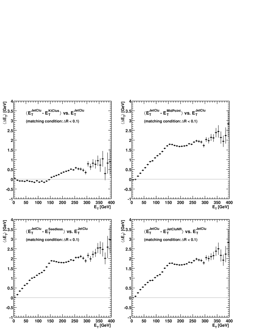
Figure 17: Difference of $E_{T}$ for matched jets found with various jet algorithms and compared to the JetClu CDF Run I algorithm. The events studied were generated with HERWIG 6.1 and run through the CDF detector simulation.

From these results we can draw several conclusions. First, the $k_{T}$ Algorithm identifies jets with $E_{T}$ values similar to those found by JetClu, finding slightly more energetic jets at small $E_{T}$ and somewhat less energetic jets at large $E_{T}$. We will not discuss this algorithm further here except to note that DØ has applied it in a study of Run I data [290] and in that analysis the $k_{T}$ Algorithm jets seem to exhibit slightly larger $E_{T}$ than expected from NLO perturbation theory. The cone algorithms, including the JetClu Algorithm without ratcheting, which is labeled JetCluNR, identify jets with approximately 0.5 % to 1 % smaller $E_{T}$ values than those identified by the JetClu Algorithm (with ratcheting), with a corresponding approximately 5 % smaller jet cross section at a given $E_{T}$ value. We believe that this systematic shortfall can be understood as resulting from the smearing effects of perturbative showering and non-perturbative hadronization.

To provide insight into the issues raised by Fig. 17 we now discuss a simple, but informative analytic picture. It will serve to illustrate the impact of showering and hadronization on the operation of jet algorithms. We consider the scalar function $F(\overrightarrow{r})$ defined as a function of the 2-dimensional variable $\overrightarrow{r}=(\eta,\phi)$ by the integral over the transverse energy distribution of either the partons or the hadrons/calorimeter towers in the final state with the indicated weight function,

$$F(\overrightarrow{r}) = \frac{1}{2}\int d^{2}\rho\;E_{T}(\overrightarrow{\rho})\cdot\left(R^{2}-(\overrightarrow{\rho}-\overrightarrow{r})^{2}\right)\cdot\Theta\left(R^{2}-(\overrightarrow{\rho}-\overrightarrow{r})^{2}\right)$$

$$= \frac{1}{2}\sum_{i}E_{T,i}\cdot\left(R^{2}-(\overrightarrow{\rho_{i}}-\overrightarrow{r})^{2}\right)\cdot\Theta\left(R^{2}-(\overrightarrow{\rho_{i}}-\overrightarrow{r})^{2}\right).$$

The second expression arises from replacing the continuous energy distribution with a discrete set, $i=1\,...\,N$, of delta functions, representing the contributions of either a configuration of partons or a set of calorimeter towers (and hadrons). Each parton direction or the location of the center of each calorimeter tower is defined in $\eta$, $\phi$ by $\rho_{i}=(\eta_{i},\phi_{i})$, while the parton/calorimeter cell has a transverse energy (or $E_{T}$) content given by $E_{T,i}$. This function is clearly related to the energy in a cone of size $R$ containing the towers whose centers lie within a circle of radius $R$ around the point $\overrightarrow{r}$. More importantly it carries information about the locations of “stable” cones. The points of equality between the $E_{T}$ weighted centroid and the geometric center of the cone correspond precisely to the maxima of $F$. The gradient of this function has the form (note that the delta function arising from the derivative of the theta function cannot contribute as it is multiplied by a factor equal to its argument)

$$\overrightarrow{\nabla}F(\overrightarrow{r})=\sum_{i}E_{T,i}\cdot(\overrightarrow{\rho_{i}}-\overrightarrow{r})\cdot\Theta\left(R^{2}-(\overrightarrow{\rho_{i}}-\overrightarrow{r})^{2}\right).$$ (181)

This expression vanishes at points where the weighted centroid coincides with the geometric center, i.e., at points of stability (and at minima of $F$, points of extreme instability). The corresponding expression for the energy in the cone centered at $\overrightarrow{r}$ is

$$E_{C}(\overrightarrow{r})=\sum_{i}E_{T,i}\cdot\Theta\left(R^{2}-(\overrightarrow{\rho_{i}}-\overrightarrow{r})^{2}\right).$$ (182)

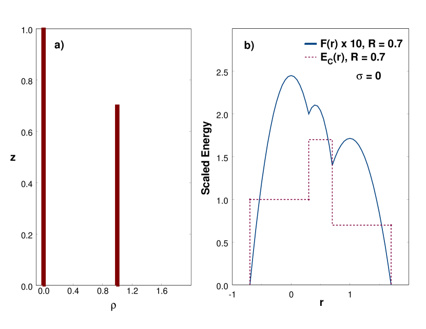
Figure 18: 2-Parton distribution: a) transverse energy distribution; b) distributions $F(r)$ and $E_{C}(r)$ in the perturbative limit of no smearing.

To more easily develop our understanding of these equations consider a simplified scenario (containing all of the interesting effects) involving 2 partons separated in just one angular dimension $\overrightarrow{\rho}\rightarrow\rho$ ($\overrightarrow{r}\rightarrow r$) with $\rho_{2}-\rho_{1}=d$. It is sufficient to specify the energies of the 2 partons simply by their ratio, $z=E_{2}/E_{1}\leq 1$. Now we can study what sorts of 2 parton configurations yield stable cones in this 2-D phase space specified by $0\leq z\leq 1$, $0\leq d\leq 2R$ (beyond $2R$ the 2 partons are surely in different cones). As a specific example consider the case $\rho_{1}=0$, $\rho_{2}=d=1.0$ and $z=0.7$ with $R=0.7$ (the typical experimental value). The underlying energy distribution is illustrated in Fig. 18a, representing a delta function at $\rho=0$ (with scaled weight 1) and another at $\rho=1.0$ (with scaled weight 0.7). This simple distribution leads to the functions $F(r)$ and $E_{C}(r)$ indicated in Fig. 18b. In going from the true energy distribution to the distribution $E_{C}(r)$ the energy is effectively smeared over a range given by $R$. In $F(r)$ the distribution is further shaped by the quadratic factor $R^{2}-(\rho_{i}-r)^{2}$. We see that $F(r)$ exhibits 3 local maxima corresponding to the expected stable cones around the two original delta functions ($r_{1}=0$, $r_{2}=1$), plus a third stable cone in the middle ($r_{3}=zd/(1+z)=0.41$ in the current case). This middle cone includes the contributions from both partons as indicated by the magnitude of the middle peak in the function $E_{C}(r)$. Note further that the middle cone is found at a location where there is initially no energy in Fig. 18a, and thus no seeds. One naively expects that such a configuration is not identified as a stable cone by the experimental implementations of the cone algorithm that use seeds simply because they do not look for it. Note also that, since both partons are entirely within the center cone, the overlap fractions are unity and the usual merging/splitting routine will lead to a single jet containing all of the initial energy ($1+z$). This is precisely how this configuration was treated in the NLO perturbative analysis of the Snowmass Algorithm [291, 292, 293, 294], i.e., only the leading jet, the middle cone, was kept).

Similar reasoning leads to Fig. 19a, which indicates the various 2 parton configurations found by the perturbative cone algorithm. For $d<R$ one finds a single stable cone and a single jet containing both partons. For $R<d<(1+z)R$ one finds 3 stable cones that merge to 1 jet, again with all of the energy. For $d>(1+z)R$ we find 2 stable cones and 2 jets, each containing one parton, of scaled energies $1$ and $z$. Thus, except in the far right region of the graph, the 2 partons are always merged to form a single jet.

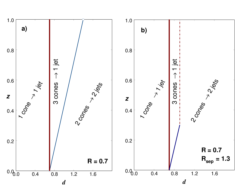
Figure 19: Perturbation Theory Structure: a) $R_{sep}=2$; b) $R_{sep}=1.3$.

We expect that the impact of seeds in experimental algorithms can be (crudely) simulated in the NLO calculations [282, 283, 284] by including a parameter $R_{sep}$ such that stable cones containing 2 partons are not allowed for partons separated by $d>R_{sep}\cdot R$. As a result cones are no longer merged in this kinematic region. In the present language this situation is illustrated in Fig. 19b corresponding to $R_{sep}=1.3$, $R\cdot R_{sep}=0.91$. This specific value for $R_{sep}$ was chosen [282, 283, 284] to yield reasonable agreement with the Run I data. The conversion of much the “3 cones $\rightarrow$ 1 jet” region to “2 cones $\rightarrow$ 2 jets” has the impact of lowering the average $E_{T}$ of the leading jet and hence the jet cross section at a fixed $E_{T,J}$. Parton configurations that naively produced jets with energy characterized by $1+z$ now correspond to jets of maximum energy 1. This is just the expected impact of a jet algorithm with seeds. Note that with this value of $R_{sep}$ the specific parton configuration in Fig. 18a will yield 2 jets (and not 1 merged jet) in the theoretical calculation. As mentioned earlier this issue is to be addressed by the Midpoint and Seedless Algorithms in Run II. However, as indicated in Fig. 17, neither of these two algorithms reproduces the results of JetClu. Further, they both identify jets that are similar to JetClu without ratcheting. Thus we expect that there is more to this story.

As suggested earlier, a major difference between the perturbative level, with a small number of partons, and the experimental level of multiple hadrons is the smearing that results from perturbative showering and nonperturbative hadronization. For the present discussion the primary impact is that the starting energy distribution will be smeared out in the variable $r$. We can simulate this effect in our simple model using gaussian smearing, i.e., we replace the delta functions in Eq. (4.1) with gaussians of width $\sigma$. (Since this corresponds to smearing in an angular variable, we would expect $\sigma$ to be a decreasing function of $E_{T}$, i.e., more energetic jets are narrower. We also note that this naive picture does not include the expected color coherence in the products of the showering/hadronization process.) The first impact of this smearing is that some of the energy initially associated with the partons now lies outside of the cones centered on the partons. This effect, typically referred to as “splashout” in the literature, is (exponentially) small in this model for $\sigma<R$. Here we will focus on less well known but phenomenologically more relevant impacts of splashout. The distributions corresponding to Fig. 18b, but now with $\sigma=0.10$ (instead of $\sigma=0$), are exhibited in Fig. 20a.

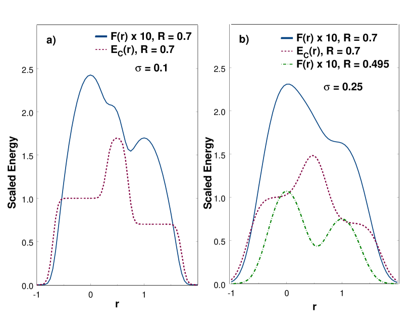
Figure 20: The distributions $F(r)$ and $E_{C}(r)$ for smearing width a) 0.1; b) 0.25.

With the initial energy distribution smeared by $\sigma$, the distribution $F(r)$ is now even more smeared and, in fact, we see that the middle stable cone (the maximum in the middle of Fig. 18b) has been washed out by the increased smearing. Thus the cone algorithm applied to data (where such smearing is present) may not find the middle cone that is present in perturbation theory, not only due to the use of seeds but also due to this new variety of splashout correction, which renders this cone unstable. Since, as a result of this splashout correction, the middle cone is not stable, this problem is not addressed by either the Midpoint Algorithm or the Seedless Algorithm. Both algorithms may look in the correct place, but they look for stable cones. This point is presumably part of the explanation for why both of these algorithms disagree with the JetClu results in Fig. 17.

Our studies also suggest a further impact of the smearing of showering/hadronization that was previously unappreciated. This new effect is illustrated in Fig. 20b, which shows $F(r)$, still for $z=0.7$ and $d=1.0$, but now for $\sigma=0.25$. With the increased smearing the second stable cone, corresponding to the second parton, has now also been washed out, i.e., the right hand local maximum has also disappeared. This situation is exhibited in the case of “data” by the lego plot in Fig. 21 indicating the jets found by the Midpoint Algorithm in a specific Monte Carlo event. The Midpoint Algorithm does not identify the energetic towers (shaded in black) to the right of the energetic central jet as either part of that jet or as a separate jet, i.e., these obviously relevant towers are not found to be in a stable cone. The iteration of any cone containing these towers invariably migrates to the nearby higher $E_{T}$ towers.

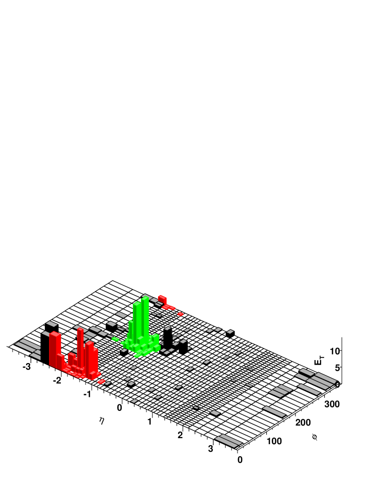
Figure 21: Result of applying the Midpoint Algorithm to a specific Monte Carlo event in the CDF detector.

In summary, we have found that the impact of smearing and splashout is expected to be much more important than simply the leaking of energy out of the cone. Certain stable cone configurations, present at the perturbative level, can disappear from the analysis of real data due to the effects of showering and hadronization. This situation leads to corrections to the final jet yields that are relevant to our goal of 1 % precision in the mapping between perturbation theory and experiment. Compared to the perturbative analysis of the 2-parton configuration, both the middle stable cone and the stable cone centered on the lower energy parton can be washed out by smearing. Further, this situation is not addressed by either the Midpoint Algorithm or the Seedless Algorithm. One possibility for addressing the missing middle cone would be to eliminate the stability requirement for the added midpoint cone in the Midpoint Algorithm. However, if there is enough smearing to eliminate also the second (lower energy) cone, even this scenario will not help, as we do not find two cones to put a third cone between. There is, in fact, a rather simple “fix” that can be applied to the Midpoint Algorithm to address this latter form of the splashout correction. We can simply use 2 values for the cone radius $R$, one during the search for the stable cones and the second during the calculation of the jet properties. As a simple example, the 3rd curve in Fig. 20b corresponds to using $R/\sqrt{2}=0.495$ during the stable cone discovery phase and $R=0.7$ in the jet construction phase. Thus the $R/\sqrt{2}$ value is used only during iteration; the cone size is set to $R$ right after the stable cones have been identified and the larger cone size is employed during the splitting/merging phase. By comparing Figs. 20b and 18b we see that the two outer stable cones in the perturbative case are in essentially the same locations as in the smeared case using the smaller cone during discovery. The improved agreement between the JetClu results and those of the Midpoint Algorithm with the last “fix” (using the smaller $R$ value during discovering but still requiring cones to be stable) are indicated in Fig. 22.

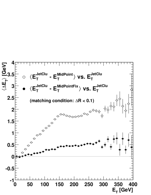
Figure 22: The difference in the $E_{T}$ of identified central jets for the JetClu and Midpoint Algorithms, both with and without the “fix” discussed in the text. The events studied were generated with HERWIG 6.1 and run through the CDF detector simulation.

Clearly most, but not all, of the differences between the jets found by the JetClu and Midpoint Algorithms are removed in the fixed version of the latter. The small $R$ “fix” suggested for the Midpoint Algorithm can also be employed for the Seedless Algorithm but, like the Midpoint Algorithm, it will still miss the middle (now unstable) cone.

Before closing this brief summary of our results, we should say a few more words about the Run I CDF algorithm that we used as a reference. In particular, while ratcheting is difficult to simulate in perturbation theory, we can attempt to clarify how it fits into the current discussion. As noted above, the JetClu Algorithm is defined so that calorimeter towers initially found around a seed stay with that cone, even as the center of the cone migrates due to the iteration of the cone algorithm. For the simple scenario illustrated in Fig. 18a we assume that the locations of the partons are identified as seeds, even when smearing is present. To include both ratcheting and the way it influences the progress of the stable cone search, we must define 2 scalar functions of the form of Eq. (4.1), one to simulate the search for a stable cone starting at $\rho=0$ and the second for the search starting at $\rho=1.0$. The former function is defined to include the energy within the range $-R\leq\rho\leq+R$ independent of the value of $r$, while the second function is defined to always include the energy in the range $1.0-R\leq\rho\leq 1.0+R$. Analyzing the two functions defined in this way suggests, as expected, that the search that begins at the higher energy seed will always find a stable cone at the location of that seed, independent of the amount of smearing. (If the smearing is small, there is also a stable cone at the middle location but the search will terminate after finding the initial, nearby stable cone.) The more surprising result arises from analyzing the second function, which characterizes the search for a stable cone seeded by the lower energy parton. In the presence of a small amount of smearing this function indicates stable cones at both the location of the lower energy parton and at the middle location. Thus the corresponding search finds a stable cone at the position of the seed and again will terminate before finding the second stable cone. When the smearing is large enough to wash out the stable cone at the second seed, the effect of ratcheting is to ensure that the search still finds a stable cone at the middle location suggested by the perturbative result, $r_{3}=z\rho/(1+z)$ (with a precision given by $\sigma\cdot e^{-(R/\sigma)^{2}}$). This result suggests that the JetClu Algorithm with ratcheting always identifies either stable cones at the location of the seeds or finds a stable cone in the middle that can lead to merging (in the case of large smearing). It is presumably just these last configurations that lead to the remaining difference between the JetClu Algorithm results and those of the “fixed” Midpoint Algorithm illustrated in Fig. 22. We find that the jets found by the JetClu Algorithm have the largest $E_{T}$ values of any of the cone jet algorithms, although the JetClu Algorithm still does not address the full range of splashout corrections.

In conclusion, we have found that the corrections due to the splashout effects of showering and hadronization result in unexpected differences between cone jet algorithms applied to perturbative final states and applied to (simulated) data. With a better understanding of these effects, we have defined steps that serve to improve the experimental cone algorithms and minimize these corrections. Further studies are required to meet the goal of 1 % agreement between theoretical and experimental applications of cone algorithms.

4.2 Comparison of PYTHIA and DIPHOX for ${\gamma\gamma}$ and $\pi^{0}\gamma$ productions

Photon pair production plays a prominent role in the search for a neutral Higgs boson at the LHC. In this respect it is relevant to directly compare the extensively used code PYTHIA [295] with a recent next–to–leading order (NLO) code DIPHOX [296]. DIPHOX is a computer code of partonic event generator type, describing the production of pairs of particles in hadronic collisions at full NLO accuracy. PYTHIA is a computer code of hadronic event generator type which fully describes an hadron-hadron collision at leading–order (LO) accuracy. The comparisons performed for the production of $\gamma\gamma$ and $\pi^{0}\gamma$ are presented in subsects. 4.2.1 and 4.2.2 respectivelly.

4.2.1 Comparison of PYTHIA and DIPHOX for ${\gamma\gamma}$ production

Here, PYTHIA version 6.152 [295] is compared to DIPHOX for the ${\gamma\gamma}$ production and K-factors are extracted. The scales used for PYTHIA are the default ones, whereas for DIPHOX all the scales have been chosen as $\sqrt{{p_{T\,\gamma_{1}}}+{p_{T\,\gamma_{2}}}}$. Note that a K-factor depends, among other things, on the factorization and renormalization scale chosen and must be used with care. In order to make easier the comparison, the direct contribution of the ${\gamma\gamma}$ production (c.f. [296]) has been split into two parts.

• A first part, called“initial direct”, groups together terms which have no final state collinear singularities. It contains the Born term $q+\bar{q}\rightarrow\gamma+\gamma$, related higher order term $q+\bar{q}\rightarrow\gamma+\gamma+g$ and the box term $g+g\rightarrow\gamma+\gamma$.

• A second part, called “Bremsstrahlung”, contains the left-over term of the direct contribution, i.e. $q+g\rightarrow\gamma+\gamma+q$ and the LO terms of the one fragmentation contribution: $q+g\rightarrow\gamma+q$, $q+\bar{q}\rightarrow\gamma+g$ where the $q/g$ fragments into a photon.

a) The initial direct contribution

a1) Comparison of PYTHIA without ISR/FSR and hadronisation with DIPHOX at LO
For this comparison, the CTEQ5L partonic densities and ${\alpha_{s}}$ at 1 loop are used. To start with, a symmetric cut is applied on the transverse momentum of the two photons ${p_{T\,\gamma}}>20$ GeV. Then more realistic cuts (the ${H\rightarrow\gamma\gamma}$ selection cuts) have been applied: $|{\eta_{\gamma}}|<2.5$, ${p_{T\,\gamma_{1}}}>40$ GeV, ${p_{T\,\gamma_{2}}}>25$ GeV. As shown in Table 7 PYTHIA and DIPHOX agree at the few percent level. The distributions of the variables ${\eta_{\gamma}}$, ${p_{T\,\gamma}}$ and ${M_{\gamma\gamma}}$ also agree well.

	${p_{T\,\gamma}}>20$ GeV		${H\rightarrow\gamma\gamma}$ selection cuts
	PYTHIA	DIPHOX	PYTHIA	DIPHOX
Born	82.3	83.2	10.2	9.8
Box	82.3	83.2	5.7	5.6
Total	164.6	166.4	15.9	15.5

Table 7: Comparison of DIPHOX and PYTHIA cross sections (in pb) for the Born and the Box terms with minimal cuts (${p_{T\,\gamma}}>20$ GeV) and after ${H\rightarrow\gamma\gamma}$ selection cuts.

a2) NLO corrections to Born
The K-factor K_NLO/LO is defined as the ratio of the NLO to the LO cross sections obtained with DIPHOX. The CTEQ5L pdf and ${\alpha_{s}}$ at 1 loop have been used to compute the LO cross section whereas the CTEQ5M pdf and ${\alpha_{s}}$ at 2 loops have been used to compute the NLO cross section. The Table 8 gives the value of the cross sections and of K_NLO/LO for different stages of the ${H\rightarrow\gamma\gamma}$ selection.

Cut	LO	NLO	KNLO/LO
${p_{T\,\gamma}}>20$ GeV	83.2	94.9	1.14
+ $|{\eta_{\gamma}}|<2.5$	32.5	41.0	1.26
+ ${p_{T\,\gamma}}>25$ GeV	18.8	23.6	1.26
+ Max(${p_{T\,\gamma_{1}}}$,${p_{T\,\gamma_{2}}}$)$>$40 GeV	5.7	10.4	1.83

Table 8: Comparison of LO and NLO cross section (in pb) for the Born term at different stage of the ${H\rightarrow\gamma\gamma}$ selection.

The asymmetric cut results in an enhancement of the K-factor. The reason is the following: at LO the two photons have the same $p_{T}$ whereas this is not the case at NLO because the $p_{T}$ balance is distorted. Therefore, at LO, the cut Max(${p_{T\,\gamma_{1}}}$,${p_{T\,\gamma_{2}}}$)$>$40 GeV is equivalent to a symmetric cut of 40 GeV on both photons. This cut acts more efficiently on LO than on NLO contributions. After all selection cuts, and if one restricts in addition to ${M_{\gamma\gamma}}>90$ GeV, K_NLO/LO is independent of ${M_{\gamma\gamma}}$ and is equal to 1.57.

ATLAS and CMS have based their prediction on PYTHIA with ISR. In order to obtain the correction which has to be applied to their numbers (K_NLO/ISR) we have compared PYTHIA with ISR to DIPHOX at NLO. The cross sections are given in Table 9. PYTHIA with ISR includes part of the NLO corrections; therefore the effect of the asymmetric cut on ${p_{T\,\gamma}}$ is reduced and K_NLO/ISR is smaller than K_NLO/LO. Since there is no hard radiation in PYTHIA, the cross section in the high $q_{T}$ region is underestimated as is shown in Fig. 24.

Cut	PYTHIA with ISR	DIPHOX at NLO	KNLO/ISR
${p_{T\,\gamma}}>20$ GeV	68.8	94.9	1.38
+ $|{\eta_{\gamma}}|<2.5$	27.6	41.0	1.49
+ ${p_{T\,\gamma}}>25$ GeV	16.0	23.6	1.48
+ Max(${p_{T\,\gamma_{1}}}$,${p_{T\,\gamma_{2}}}$)$>$40 GeV	6.9	10.4	1.51

Table 9: Comparison of PYTHIA (CTEQ5L+ ${\alpha_{s}}$ at 1 loop) with ISR and DIPHOX NLO cross section (in pb) for the Born term at different stage of the ${H\rightarrow\gamma\gamma}$ selection.

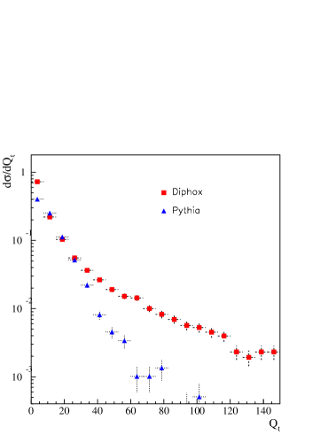
Figure 23: $Q_{t}$ distribution for PYTHIA with ISR and DIPHOX NLO after all selection cuts for the Born contribution.

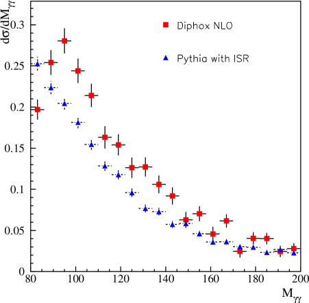
Figure 24: ${M_{\gamma\gamma}}$ distribution for PYTHIA with ISR and DIPHOX NLO after all selection cuts for the Born plus Box contribution.

a3) The Box contribution
Since there is no higher order calculation for the Box contribution, we have studied the effect of switching on ISR and of including the running of ${\alpha_{s}}$ at 2 loops. PYTHIA with ISR results in a cross section larger by 40$\%$ after all selection cuts. This increase is again an effect of the asymmetric cuts. For ${M_{\gamma\gamma}}>80$ GeV the ratio is equal to 1.19. The inclusion of ${\alpha_{s}}$ at 2 loops decreases the cross section by $23\%$. Therefore, the effect of including ISR in PYTHIA almost cancels the effect of the running of ${\alpha_{s}}$. Thus we keep the LO calculation with ${\alpha_{s}}$ at one loop for the DIPHOX ’NLO’ calculation in the following.

a4) K-factor for the direct ${\gamma\gamma}$ production
In this section, we compare the cross sections obtained by PYTHIA with ISR (which correspond to the experiment’s Monte–Carlo) to the NLO prediction from DIPHOX for the direct ${\gamma\gamma}$ production (i.e. Born plus Box). PYTHIA is used with CTEQ5L and ${\alpha_{s}}$ at 1 loop. The DIPHOX ’NLO’ contribution includes Born at NLO with CTEQ5M and ${\alpha_{s}}$ at 2 loops (as in a2)) and Box at LO with CTEQ5L and ${\alpha_{s}}$ at 1 loop (as in a3)). The cross sections are given in Table 10 and Fig. 24 shows the ${M_{\gamma\gamma}}$ distribution after all selection cuts for PYTHIA and DIPHOX.

Cut	PYTHIA with ISR			DIPHOX ’NLO’			KNLO/ISR
	Box	Born	Total	Box	Born	Total
${p_{T\,\gamma}}>20$ GeV	60.3	68.8	129.1	83.2	94.9	178.1	1.38
+ $|{\eta_{\gamma}}|<2.5$	41.4	27.6	69.0	56.3	41.0	97.3	1.41
+ ${p_{T\,\gamma}}>25$ GeV	18.9	16.0	34.9	25.7	23.6	49.3	1.41
+ Max(${p_{T\,\gamma_{1}}}$,${p_{T\,\gamma_{2}}}$)$>$40 GeV	6.6	6.9	13.5	4.7	10.4	15.1	1.12
+ ${M_{\gamma\gamma}}>80$GeV	5.6	6.4	12.0	4.7	9.5	14.2	1.18

Table 10: Comparison of PYTHIA (CTEQ5L+ ${\alpha_{s}}$ at 1 loop) with ISR and DIPHOX ’NLO’ cross section (in pb) at different stage of the ${H\rightarrow\gamma\gamma}$ selection for Born plus Box contributions. The K factor is the ratio of the total cross sections for PYTHIA with ISR and DIPHOX ’NLO’.

b) The Bremsstrahlung contribution
In PYTHIA the Bremsstrahlung contribution is obtained with the processes $qg\rightarrow q\gamma$ and $q\bar{q}\rightarrow g\gamma$ with QCD ISR and FSR. The second photon is produced mainly by QED FSR. The cross sections are summarized in Table 11. Note that the isolation cut reduces the cross section by less than a factor 2. All the cross sections are obtained with CTEQ5L and ${\alpha_{s}}$ at 1 loop. ISR/FSR in PYTHIA does not produce as high ${p_{T\,\gamma}}$ as DIPHOX NLO, therefore the cross section is smaller in PYTHIA. Moreover the asymmetric cut on ${p_{T\,\gamma}}$ enhances this difference: since PYTHIA is a quasi $2\rightarrow 2$ generator it does not produce high $p_{T}$ difference between the photons.
An isolation cut is defined by imposing that $\Delta R>0.4$ or ${p_{T\,p}}<10$ GeV. For DIPHOX, ${p_{T\,p}}$ is either the $p_{T}$ of the parton $p$ produced with the photon pair or the transverse energy of the residue of the fragmentation flowing along the photon direction. $\Delta R$ is the smallest distance between the parton $p$ produced with the photon pair and the photons , $\Delta R=\rm{Min}((\eta_{p}-\eta_{\gamma_{1,2}})^{2}+(\phi_{p}-\phi_{\gamma_{1,2}})^{2})$. For PYTHIA, ${p_{T\,p}}=||\sum_{i}\vec{p}_{T\,i}||$ where the sum runs on all the partons produced in the shower going with the photon and $\Delta R$ is the smallest distance in rapidity-azimuthal angle plane between the parton produced in the $2\rightarrow 2$ hard scattering and the photons. The isolation cut also slightly enhances the K-factor. It might be due to the fact that the quark tends to be more collinear to the radiated photon in PYTHIA. Figure 26 shows the ${M_{\gamma\gamma}}$ distribution after all selection cuts and Figure 26 shows the $q_{T}$ distribution.

Cut	PYTHIA (ISR/FSR)	DIPHOX	K${}^{\rm{brem}}_{\rm{DIPHOX/PYTHIA}}$
$|{\eta_{\gamma}}|<2.5$, ${p_{T\,\gamma}}>25$ GeV	22.2	27.5	1.24
+ Max(${p_{T\,\gamma_{1}}}$,${p_{T\,\gamma_{2}}}$)$>$40 GeV	14.9	24.7	1.66
+ ${M_{\gamma\gamma}}>80$GeV	11.9	19.7	1.66
$\Delta r>0.4$ or ${p_{T\,p}}<10$ GeV	7.4	12.8	1.72

Table 11: Comparison of PYTHIA (CTEQ5L+ ${\alpha_{s}}$ at 1 loop) with ISR/FSR and DIPHOX cross section (in pb) at different stage of the ${H\rightarrow\gamma\gamma}$ selection for the Bremsstrahlung contribution.

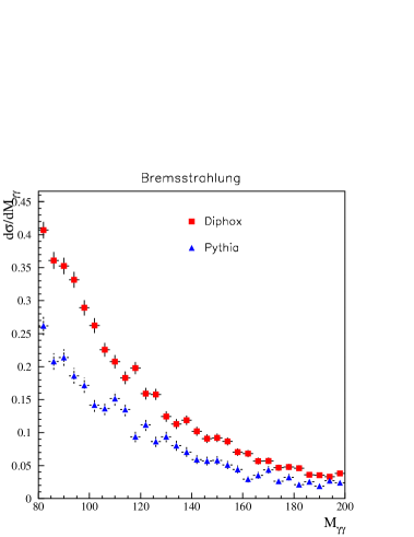
Figure 25: ${M_{\gamma\gamma}}$ distribution for PYTHIA and DIPHOX after all selection cuts for the Bremsstrahlung contribution.

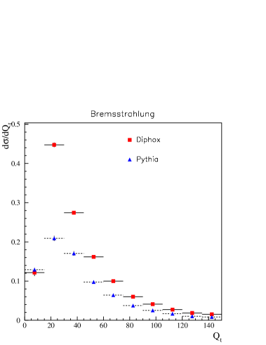
Figure 26: $Q_{t}$ distribution for PYTHIA and DIPHOX after all selection cuts for the Bremsstrahlung contribution.

Conclusion
The contribution of the two photon background for the $H\rightarrow{\gamma\gamma}$ search at the LHC has been estimated at NLO with DIPHOX and compared to PYTHIA Monte–Carlo. The K-factor has to be used with care since it depends on the selection cuts notably on the isolation criteria. Note that the asymmetric cut on ${p_{T\,\gamma}}$ is responsible for an enhancement of the K-factor.

4.2.2 Comparison of PYTHIA and DIPHOX for $\pi^{0}\,\gamma$ production

Because of the huge jet rates at the LHC, any photonic observable is heavily contaminated by neutral pions which appear as fake photons inside the electro-magnetic calorimeter. Thus, concerning the search for a light neutral Higgs boson in the mass window between 80 to 140 GeV, a detailed understanding of not only $\gamma\gamma$ but also $\gamma\pi^{0}$ and $\pi^{0}\pi^{0}$ rates is mandatory [297, 298, 299, 300, 301, 302]. The experimental studies for LHC depend heavily on Monte–Carlo event generators like PYTHIA which treat QCD observables on the leading order level along with the modelling of hadronization and radiation effects. A comparison with theoretical results which include up-to-date knowledge is a way to test the reliability of these programs. An adequate tool to do such a comparison is the DIPHOX code which is a partonic event generator designed for the pair production of hadrons and/or photons in hadronic collisions at full next–to–leading order [296, 303].

Here we present a comparison of $\pi^{0}\gamma$ observables relevant for Higgs search, namely the invariant mass, $M_{\gamma\pi}$ and the transverse momentum distribution of the pair, $q_{T}$, with a special emphasis on isolation criteria. Both distributions were calculated with PYTHIA 6.152[295] and DIPHOX. In the former, in order to allow a comparison, the multiple interactions within the p-p collision were switched off and the pile-up effects from the collisions within the same bunch crossing were not taken into account. The comparisons were made with the initial and final state radiation allowed.

Two isolation criteria were implemented: the transverse energy flow isolation and the charged track isolation. In the former, a threshold is set to the sum of $E_{T}$ of all particles in the isolation cone $\Delta R=\sqrt{(\Delta\eta)^{2}+(\Delta\phi)^{2}}$. In the latter, a threshold is set to the maximum $p_{T}$ of any charged particle in the isolation cone. The correlation between the two isolation criteria is plotted in Fig. 27.

Figure 27: Comparison between the cone isolation criterion vs. charged track isolation.

As DIPHOX generates only partonic events with a subsequent collinear fragmentation of partons into pions, only the transverse energy flow isolation can be implemented. From Fig. 27 it can be inferred that the maximal hadronic transverse energy inside a cone lies between 5 and 15 GeV in an experimentally realistic situation. As a reminder, this is the transverse energy stemming from the partonic reaction only and not from multiple interactions and/or pile-up. In this window, the partonic reaction, $qg\rightarrow q\gamma$, is by far dominant in the cross section. This motivates us to focus on this case only. For the following plots we fixed the isolation cone size to be $\Delta R=0.4$.

With PYTHIA the process $q+g\rightarrow q+\gamma$ was generated and a requirement was made that the photon candidates (real photon or a hard $\pi^{0}$ from the quark jet) have $p_{T}>$ 25, 40 GeV, and that they are within the pseudo-rapidity range of $|\eta|<2.5$. A invariant mass cut of $80\,\mbox{GeV}<M_{\pi\gamma}<140\,\mbox{GeV}$ was imposed. Furthermore, it was required that one of the photon candidates is a $\pi^{0}$, thus rejecting events were the second photon comes from the jet fragmentation. With DIPHOX the same reaction, including next-to-leading corrections, was calculated. The next-to-leading order parton distribution functions GRV94[304] were used to compare with the PYTHIA default value. Only direct photons were considered in this study, since in the case of severe isolation, the contribution from fragmentation is suppressed below the 10 per cent level. For the fragmentation scale we used the value $M_{\gamma\pi}/8$. This non-canonical choice is dictated by the fact that in the case of isolation cuts the typical fragmentation scale should be governed by values $\sim E_{Tmax}$ [305].

In Fig. 29 the comparison between PYTHIA and DIPHOX is shown for the invariant mass distribution of the pion photon pair. Good agreement is found for the case of very loose isolation, $E_{Tmax}=100$ GeV and the more relevant value of $E_{Tmax}=15$ GeV. Note that the NLO prediction is plagued by large scale uncertainties around $\pm 30$ to $40$ per cent, as the hard experimental cuts spoil compensations of higher order terms with opposite signs. In the case of very strict isolation, $E_{Tmax}=5$ GeV, PYTHIA produces somewhat higher rates. The discrepancy has presumably three sources which have to do with the small value of $E_{Tmax}$. Small $E_{Tmax}$ means that the fragmentation variable $z$, the ratio of transverse pion momentum to parent parton momentum, is pressed towards one, $z>z_{min}=p_{Tmin}/(p_{Tmin}+E_{Tmax})\sim 0.8$. In this regime, first of all, the available fragmentation functions are not well constrained by experimental data [306] and there may be differences in the fragmentation/hadronization models for large $z$ implemented in PYTHIA and DIPHOX. Second, large logarithms ($\sim\log(1-z)^{2}$) are present in the next-to-leading order calculation which may render the perturbative contributions unreliable. Third, the above mentioned fact that the fragmentation scale choice should be related to $E_{Tmax}$, indeed, indicates that the fragmentation scale should be chosen smaller here, which increases the DIPHOX prediction in the right way. With the value $M_{f}$=$M_{\gamma\pi}/16$ the DIPHOX curve shifts upwards by about 40 per cent leading to a better agreement. Altogether one can conclude that PYTHIA and DIPHOX show a reasonable agreement in the invariant mass distribution apart from the regime of very hard isolation which deserves further investigation from the theoretical side [305]. In Fig. 29, the $q_{T}$ spectrum is plotted for the same isolation criteria. For $E_{Tmax}=15,100$ GeV good agreement is found for the used scales for the first bins. The shape for these contributions is not quite the same, with the PYTHIA prediction being slightly steeper. This is to be expected, as the NLO calculation encoded in DIPHOX contains $2\rightarrow 3$ matrix elements, enhancing the tail of the distribution. As a reminder, the tail in PYTHIA is filled by a parton showering model which is not as reliable as explicit higher order matrix elements. Still, the disagreement in shape for the relevant $q_{T}$ domain seems not too alarming in the plotted range. Note that in the case of hard isolation the PYTHIA prediction of the last 4 bins is plagued by low statistics. The apparent overall discrepancy in the case $E_{Tmax}=5$ GeV can be understood by the same reasoning as given above for the $M_{\gamma\pi}$ spectrum.

Figure 28: Comparison PYTHIA vs. DIPHOX: The invariant $\gamma\pi$-mass spectrum for different cone isolation criteria and standard LHC cuts.

Figure 29: Comparison PYTHIA vs. DIPHOX: The transverse momentum spectrum of $\gamma\pi$ pairs for different cone isolation criteria and standard LHC cuts.

In conclusion, the comparison between PYTHIA and the NLO DIPHOX code shows a reasonable agreement. Whereas infrared insensitive spectra, such as the invariant mass distribution, differ only by an overall normalisation which can be accounted for by an adequate scale choice, infrared sensitive observables like the transverse momentum distribution of the pair are typically steeper in PYTHIA due to missing NLO matrix elements. In the case of very hard isolation an apparent difference between the PYTHIA and DIPHOX predictions can be traced back to a different modelling of the production of high $p_{T}$ pions, a too high fragmentation scale choice and/or subtleties in the interplay between higher order corrections and severe experimental cuts. This will be extensively discussed elsewhere [305].

5 Monte Carlo^, 

5.1 Introduction

The Monte-Carlo intergroup focused on four main issues: the problem of interfacing partonic event generators to showering Monte-Carlos, an implementation using this interface to calculate backgrounds which are poorly simulated by the showering Monte-Carlos alone, a comparison of the HERWIG and PYTHIA parton shower models with the predictions of a soft gluon resummation program (ResBos), and studies of the underlying events at hadron colliders and how well they are modeled by the Monte-Carlo generators.

Section 5.2 discusses a strategy whereby generic Fortran common blocks are presented for use by High Energy Physics event generators for the transfer of event configurations from parton level generators to showering and hadronization event generators.

Section 5.3 discusses the AcerMC Monte Carlo Event Generator which is dedicated to the generation of the Standard Model background processes at $pp$ LHC collisions. The program itself provides a library of the massive matrix elements and phase space modules for the generation of selected processes: $q\bar{q}\to W(\to\ell\nu)b\bar{b}$, $q\bar{q}\to W(\to\ell\nu)t\bar{t}$, $gg,q\bar{q}\to Z/\gamma^{*}(\to\ell\ell)b\bar{b}$, $gg,q\bar{q}\to Z/\gamma^{*}(\to\ell\ell,\nu\nu,b\bar{b})t\bar{t}$, the QCD $gg,q\bar{q}\to t\bar{t}b\bar{b}$ and EW $gg\to(Z/W/\gamma\to)t\bar{t}b\bar{b}$. The hard process event, generated with these modules, can be completed by the initial and final state radiation, hadronization and decays, simulated with either the PYTHIA or HERWIG Monte Carlo Event Generators. Interfaces to both these generators are provided in the distribution version. The AcerMC also uses several other external libraries: CERNLIB, HELAS, VEGAS.

In Section 5.4, predictions for the $p_{T}$ distribution for a Higgs particle were generated using two approaches: (1) a soft-gluon resummation technique, using the program ResBos and (2) a parton shower technique using the Monte Carlo programs HERWIG and PYTHIA. An understanding of the kinematics of the Higgs boson, or of any other Standard Model or non- Standard Model particle, and the characteristics of any jets associated with its production, is of great interest for physics at the Tevatron, the LHC or any future hadron colliders. The transverse momentum distribution of the Higgs boson depends primarily on the details of the soft gluon emission from the initial state partons. The effects of these soft gluon emissions can be described either by a resummation calculation or by a Monte Carlo parton shower formalism. Comparisons between the two techniques for several different Higgs masses and for several center-of-mass energies show relatively good agreement between the ResBos predictions and those of HERWIG and recent versions of PYTHIA.

In Section 5.5, the behavior of the “underlying event” in hard scattering proton-antiproton collisions at $1.8{\rm\,TeV}$ is studied and compared with the QCD Monte-Carlo models. The “hard scattering” component consists of the outgoing two “jets” plus initial and final-state radiation. The “underlying event” is everything except the two outgoing hard scattered “jets” and consists of the “beam-beam remnants” plus possible contributions from the “hard scattering” arising from initial and final-state radiation. In addition multiple parton scattering might contribute to the “underlying event”. The data indicate that neither ISAJET or HERWIG produce enough charged particles (with $p_{T}\!>\!0.5\,{\rm GeV/c}$) from the “beam-beam remnant” component and that ISAJET produces too many charged particles from initial-state radiation. The “tuning” of ISAJET and PYTHIA to fit the “underlying event” is explored.

In addition to these activities, discussions were held with the “standard model” and “beyond the standard model” groups in order to assess their needs. Many of these needs are expressed in terms of the desire to have new processes added to the showering Monte-Carlo event generators. The interface discussed in Section 5.2 should make this easier for users to implement the processes themselves, obviating the need to have the Monte-Carlo authors do it. Among the important items mentioned are:

• The production of $WZ$ final states should include the contributions from virtual $W$ and $Z$ as these are vital for SUSY searches at the Tevatron

• Resummation of the $log(m_{H}/m_{b})$ and $log(m_{H}/p_{t})$ terms in the $gg\to Hb\overline{b}$ process.

• Radion phenomenology

• A better understanding of the $gg\to H$ process and in particular the effect of a jet veto

• Correct $\tau$ polarization in Higgs decay.

5.2 Generic User Process Interface for Event Generators

Modularization of High Energy Particle Physics event generation is becoming increasingly useful as the complexity of Monte Carlo programs grows. To accommodate this trend, several authors of popular Monte Carlo and matrix element programs attending the Physics at TeV Colliders Workshop in Les Houches, 2001 have agreed on a generic format for the transfer of parton level event configurations from matrix element event generators (MEG) to showering and hadronization event generators (SHG).

CompHEP[307]
Grace[308]		HERWIG[309]
MadGraph[310]	$\Rightarrow$	ISAJET[311]
VecBos[312]		PYTHIA[313]
WbbGen[314]		…
…

Events generated this way are customarily called user (or user-defined) processes, to distinguish them from the internal processes that come with the SHG. Specific solutions are already in use, including an interface of WbbGen with HERWIG [315] and an interface of CompHEP with PYTHIA [316]—that experience is exploited here.

Since the specification of the user process interface in May 2001 at Les Houches, the interface has been (or is being) implemented in a number of MEG and SHG programs. An implementation has been included in PYTHIA 6.2, described (with an example) in Ref. [317]. A HERWIG implementation is in progress and will appear in Version 6.5. MEG implementations exist for the Madison Collection of User Processes (MADCUP) [318], ALPGEN [314, 319], and CompHEP [320] (to be available publicly soon). An implementation in MadGraph is in preparation. Other MEG implementations include Refs. [321, 322].

The user process interface discussed here is not intended as a replacement for HEPEVT [323], which is the standard Fortran common block for interface between generators and analysis/detector simulation. The user process common blocks address the communication between two event generators only, a MEG one and a SHG one, and not the communication of event generators with the outside world.

In the course of a normal event generation run, this communication occurs at two stages: (1) at initialization, to establish the basic parameters of the run as a whole and (2) for each new event that is to be transferred from the MEG to the SHG. Each of these two stages here corresponds to its own Fortran common block. These common blocks are described in detail in the next two sections, followed by some examples.

One can also foresee that each stage will be associated with its own subroutine, called from the SHG, where information is put in the respective common block, based on output from the MEG. The details of these subroutines are likely to be specific to a given MEG and may also be specific to a given SHG. The subroutine names UPINIT and UPEVNT (each with no arguments) were chosen for the PYTHIA 6.2 implementation. They are intended to be generic (the usual PY prefixes are omitted), and only dummy versions are packaged with the program. It is recommended that other SHG authors use the same dummy routine names (with zero arguments) such that for simple cases which do not require intervention ‘by hand’, MEG authors will be able to interface several SHGs with a single set of routines. Example routines are presented in the PYTHIA documentation [317].

In general, a user process run may consist of a number of subprocesses, each denoted by a unique integer identifier. If the user wishes to have the SHG unweight events using acceptance-rejection and/or mix together events from different processes, then the user process author will need to supply a subroutine that is able to return an event of the requested subprocess type to the SHG on demand. The author may choose to organize the subroutine to generate the event ‘on the fly’, or to read the event from a file stream (with a separate file stream for each subprocess). The SHG will also need information about the subprocess cross section and/or maximum event weight to select which process is generated next and for acceptance-rejection. This information will need to be known from the onset (and could, for example, be determined in advance from an initialization run). Alternatively, the user may already have a proper mixture of subprocesses from the MEG and only wish the SHG to process events in the order they are handed in. We therefore allow for several different event weight models.

If extra information is needed for a specific user implementation, then a implementation-specific common block should be created. The meaning of the user process common block elements should not be overloaded, as this would defeat the generic purpose.

The descriptions in this paper are intended for event generator authors and may appear complex—most of the details will be transparent to the casual user.

5.2.1 ‘User Process’ Run Information

The run common block contains information which pertains to a collection of events.
In general this information is process dependent and it is impossible to include everything in a generic common block. Instead only the most general information is included here, and it is expected that users will have to intervene ‘by hand’ for many cases (i.e. a user may need to specify which cutoffs are used to avoid singularities, which jet clustering algorithm has been used to recombine partons in a next-to-leading-order calculation, the effective parton masses, …).

      integer     MAXPUP
      parameter ( MAXPUP=100 )
      integer     IDBMUP, PDFGUP, PDFSUP, IDWTUP, NPRUP, LPRUP
      double precision EBMUP, XSECUP, XERRUP, XMAXUP
      common /HEPRUP/ IDBMUP(2), EBMUP(2), PDFGUP(2), PDFSUP(2),
     +                IDWTUP, NPRUP, XSECUP(MAXPUP), XERRUP(MAXPUP),
     +                XMAXUP(MAXPUP), LPRUP(MAXPUP)

HEPRUP ‘User Process’ Run Common Block

• parameter  MAXPUP=100 : maximum number of different processes to be interfaced at one time

  Beam Information
  Beam particle 1 (2) is defined as traveling along the +Z (–Z) direction.

• integer  IDBMUP(2) : ID of beam particle 1 and 2 according to the Particle Data Group convention [325]

• double  EBMUP(2) : energy in GeV of beam particles 1 and 2

• integer  PDFGUP(2) : the author group for beam 1 and 2, according to the Cernlib PDFlib [326] specification

• integer  PDFSUP(2) : the PDF set ID for beam 1 and 2, according to the Cernlib PDFlib specification
  For $e^{+}e^{-}$ or when the SHG defaults are to be used, PDFGUP=–1, PDFSUP=–1 should be specified.
  The PDFlib enumeration of PDFs is sometimes out of date, but it is the only unique integer labels for PDFs available. In the case where a PDF not included in PDFlib is being used, this information will have to be passed ‘by hand’.

  Process Information

• integer  IDWTUP : master switch dictating how the event weights (XWGTUP) are interpreted
  The user is expected to pick the most appropriate event weight model for a run, given the MEG input at hand and the desired output. Normally the SHG should be able to handle all of the models.
  A summary of the IDWTUP switches is presented in Table 12.

  • Events are weighted on input and the SHG is asked to produce events with weight +1 as output. XSECUP and XERRUP need not be provided, but are calculated by the SHG. XWGTUP is a dimensional quantity, in pb, with a mean value converging to the cross section of the process. The SHG selects the next subprocess type to be generated, based on the relative size of the XMAXUP(i) values. The user-supplied interface routine must return an event of the requested type on demand from the SHG, and the maximum weight XMAXUP (or a reasonable approximation to it) must be known from the onset. A given event is accepted with a probability XWGTUP/XMAXUP(i). In case of rejection, a new event type and a new event are selected. If XMAXUP(i) is chosen too low, such that XWGTUP violates the XMAXUP(i), the SHG will issue a warning and update XMAXUP(i) with the new maximum weight value. If events of some types are already available unweighted, then a correct mixing of these processes is ensured by putting XWGTUP = XMAXUP(i). In this option also the internal SHG processes are available, and can be mixed with the external ones. All weights are positive definite. $k$-factors may be included on an event by event basis by the user process interface by re-scaling the XWGTUP for each event.

  • Same as above (IDWTUP=+1), but the event weights may be either positive or negative on input, and the SHG will produce events with weight +1 or –1 as output. A given event would be accepted with a probability $|$XWGTUP$|$/$|$XMAXUP(i)$|$ and assigned weight sign(1,XWGTUP), where the sign function transfers the sign of XWGTUP onto 1. A physics process with alternating cross section sign must be split in two IDPRUP types, based on the sign of the cross section, such that all events of a particular IDPRUP have the same event weight sign. Also the XMAXUP(i) values must be available for these two IDPRUP types separately, so that $|$XMAXUP(i)$|$ gives the relative mixing of event types, with event acceptance based on $|$XWGTUP$|$/$|$XMAXUP(i)$|$.

  • Events are weighted on input and the SHG is asked to produce events with weight +1 as output. The SHG selects the next subprocess type to be generated, based on the relative size of the XSECUP(i) values. The user-supplied interface routine must return an event of the requested type on demand from the SHG. The cross sections XSECUP(i) must be known from the onset. A given event is accepted with a probability XWGTUP/XMAXUP(i). In case of rejection, a new event of the same type would be requested. In this scenario only the ratio XWGTUP/XMAXUP(i) is of significance. If events of some types are already available unweighted, then a correct mixing of these processes is ensured by putting XWGTUP = XMAXUP(i). A $k$-factor can be applied to each process by re-scaling the respective XSECUP(i) value at the beginning of the run, but cannot be given individually for each event. In this option also the internal SHG processes are available, and can be mixed with the user processes.

  • Same as above (IDWTUP=+2), but the event weights may be either positive or negative on input, and the SHG will produce events with weight +1 or –1 as output. A physics process with alternating cross section sign must therefore be split in two IDPRUP types, based on the sign of the cross section, such that all events of a particular IDPRUP have the same event weight sign. Also the XSECUP(i) and XMAXUP(i) values must be available for these two IDPRUP types separately, so that $|$XSECUP(i)$|$ gives the relative mixing of event types, with event acceptance based on $|$XWGTUP$|$/$|$XMAXUP(i)$|$ and the total cross section of the two IDPRUP types combined given by XSECUP(i)+XSECUP(j).

  • Events are unweighted on input such that all events come with unit weight XWGTUP=+1. The SHG will only ask for the next event. If any mixing or unweighting is desired, it will have to be performed by the user process interface. The SHG will not reject any events (unless it encounters other kinds of problems). If a $k$-factor is desired, it is the responsibility of the user process interface. When events are read sequentially from an already existing file, this would imply one common $k$-factor for all processes. In this option it is not possible to mix with internal SHG processes.

  • Same as above (IDWTUP=+3), but the event weights may be either +1 or –1 on input. A single process identifier (IDPRUP) may include events with both positive and negative event weights.

  • Same as (IDWTUP=+3), but events are weighted on input and the average of the event weights (XWGTUP) is the cross section in pb. When histogramming results on analyzed events, these weights would have to be used. The SHG will only ask for the next event and will not perform any mixing or unweighting. Neither XSECUP nor XMAXUP needs to be known or supplied. In this option it is not possible to mix with internal SHG processes.

  • Same as (IDWTUP=+4), but event weights may be either positive or negative on input and the average of the event weights (XWGTUP) is the cross section. A single process identifier (IDPRUP) may include events with both positive and negative event weights.

  	event selection	control of	XWGTUP
  IDWTUP	according to	mixing/unweighting	input	output
  +1	XMAXUP	SHG	+ weighted	+1
  –1	XMAXUP	SHG	$\pm$ weighted	$\pm$1
  +2	XSECUP	SHG	+ weighted	+1
  –2	XSECUP	SHG	$\pm$ weighted	$\pm$1
  +3	—	user interface	+1	+1
  –3	—	user interface	$\pm$1	$\pm$1
  +4	—	user interface	+ weighted	+ weighted
  –4	—	user interface	$\pm$ weighted	$\pm$ weighted

  Table 12: Summary of the options available for the master weight switch IDWTUP.

• integer  NPRUP : the number of different user subprocesses
  i.e. LPRUP and other arrays will have NPRUP entries, LPRUP(1:NPRUP)

• double  XSECUP(J) : the cross section for process J in pb
  This entry is mandatory for IDWTUP=$\pm$2.

• double  XERRUP(J) : the statistical error associated with the cross section of process J in pb
  It is not expected that this information will be used by the SHG, except perhaps for printouts.

• double  XMAXUP(J) : the maximum XWGTUP for process J
  For the case of weighted events (IDWTUP=$\pm$1,$\pm$2), this entry is mandatory—though it need not be specified to a high degree of accuracy. If too small a number is specified, the SHG will issue a warning and increase XMAXUP(J). This entry has no meaning for IDWTUP=$\pm$3,$\pm$4.

• integer  LPRUP(J) : a listing of all user process IDs that can appear in IDPRUP of HEPEUP for this run
  When communicating between the user process and SHG, the LPRUP code will be used. Example: if LPRUP(1)=1022, then the SHG will ask for an event of type 1022, not 1.

 

5.2.2 ‘User Process’ Event Information

      integer MAXNUP
      parameter ( MAXNUP=500 )
      integer NUP, IDPRUP, IDUP, ISTUP, MOTHUP, ICOLUP
      double precision XWGTUP, SCALUP, AQEDUP, AQCDUP,
     +                 PUP, VTIMUP, SPINUP
      common /HEPEUP/ NUP, IDPRUP, XWGTUP, SCALUP, AQEDUP, AQCDUP,
     +                IDUP(MAXNUP), ISTUP(MAXNUP), MOTHUP(2,MAXNUP),
     +                ICOLUP(2,MAXNUP), PUP(5,MAXNUP), VTIMUP(MAXNUP),
     +                SPINUP(MAXNUP)

HEPEUP ‘User Process’ Event Common Block

• parameter  MAXNUP=500 : maximum number of particle entries

• integer  NUP : number of particle entries in this event
  An event with NUP=0 denotes the case where the user process is unable to provide an event of the type requested by the SHG (i.e. if the user process is providing events to the SHG by reading them sequentially from a file and the end of the file is reached).

• integer  IDPRUP : ID of the process for this event
  The process ID’s are not intended to be generic. The entry is a hook which the event generators can use to translate into their own scheme, or use in print statements (e.g. so that cross section information can be shown per process).
  When IDWTUP$=\pm 1,\pm 2$ the next process to be generated is selected by the SHG, and so IDPRUP is set by the SHG. For IDWTUP$=\pm 3,\pm 4$ the process is selected by the MEG, and IDPRUP is set by the MEG.

• double  XWGTUP : event weight
  weighted events: if the user process supplies weighted events and the SHG is asked to produce unweighted events, this number will be compared against XMAXUP in the run common block HEPRUP for acceptance-rejection.
  unweighted events: if the user process supplies events which have already been unweighted, this number should be set to +1 (-1 for negative weight events in e.g. a NLO calculation).

  The precise definition of XWGTUP depends on the master weight switch IDWTUP in the run common block. More information is given there.

• double  SCALUP : scale of the event in GeV, as used for calculation of PDFs
  If the scale has not been defined, this should be denoted by setting the scale to –1.

• double  AQEDUP : the QED coupling $\alpha_{\mathrm{QED}}$ used for this event (e.g. $\frac{1}{128}$)

• double  AQCDUP : the QCD coupling $\alpha_{\mathrm{QCD}}$ used for this event

  When $\alpha_{\mathrm{QED}}$ and/or $\alpha_{\mathrm{QCD}}$ is not relevant for the process, or in the case where the user process prefers to let the SHG use its defaults, AQEDUP=–1 and/or AQCDUP=–1 should be specified.

  ID, Status, and Parent-Child History

• integer  IDUP(I) : particle ID according to Particle Data Group convention [325]
  undefined (and possibly non-physical) “particles” should be assigned IDUP=0 (i.e. the $WZ$ particle in the example given in the MOTHUP description below)

• integer  ISTUP(I) : status code

  • Incoming particle

  • Outgoing final state particle

  • Intermediate space-like propagator defining an $x$ and $Q^{2}$ which should be preserved

  • Intermediate resonance, Mass should be preserved

  • Intermediate resonance, for documentation only

  • Incoming beam particles at time $t=-\infty$

  The recoil from a parton shower (including photon emission) needs to be absorbed by particles in the event. Without special instructions, this can alter the mass of intermediate particles. The ISTUP flag +2 allows the user process to specify which intermediate states should have their masses preserved, i.e. for $e^{+}e^{-}\rightarrow Z^{0}h^{0}\rightarrow q\bar{q}b\bar{b}$, the $Z^{0}$ and $h^{0}$ would be flagged with ISTUP=+2.
  The primary application of the ISTUP=–2 status code is deep inelastic scattering (a negative number is chosen for this status code because the propagator in some sense can be thought of as incoming). See the example below.
  The status code ISTUP=–9 specifying incoming beams is not needed in most cases because the beam particle energy and identity is contained in the HEPRUP run information common block. The primary application of this status code will be non-collinear beams and/or runs for which the beam energy varies event by event (note that using the –9 status code to vary the machine energy may produce problems if the SHG is asked to combine separate processes). The use of ISTUP=–9 entries is optional, and is only necessary when the information in HEPRUP is insufficient. If entries with ISTUP=–9 are specified, this information will over-ride any information in HEPRUP.

• integer  MOTHUP(2,I) : index of first and last mother
  For decays, particles will normally have only one mother.
  In this case either MOTHUP(2,I)=0 or MOTHUP(2,I)=MOTHUP(1,I). Daughters of a $2\rightarrow n$ process have 2 mothers. This scheme does not limit the number of mothers, but in practice there will likely never be more than 2 mothers per particle.

  The history (intermediate particles) will be used by the SHGs to decipher which combinations of particles should have their masses fixed and which particle decays should be “dressed” by the parton shower. Example: for $q\bar{q}^{\prime}\rightarrow W^{-}Zg\rightarrow l^{-}\nu l^{+}l^{-}g$, intermediate “particles” $WZ$, $W$, and $Z$ could be specified with ISTUP=+2. Here the $WZ$ “particle” would have its own entry in the common block with IDUP=0. The showering generator would preserve the invariant masses of these “particles” when absorbing the recoil of the parton shower.

  In a case like $e^{+}e^{-}\rightarrow\mu^{+}\mu^{-}\gamma$ proceeding via a $\gamma^{*}/Z^{0}$, where the matrix element contains an interference term between initial and final-state emission, this ambiguity in the parent-child history of the $\gamma$ has to be resolved explicitly by the user process.

  Color Flow
  A specific choice of color flow for a particular event is often unphysical, due to interference effects. However, SHGs require a specific color state from which to begin the shower—it is the responsibility of the user process to provide a sensible choice for the color flow of a particular event.

• integer  ICOLUP(1,I) : integer tag for the color flow line passing through the color of the particle

• integer  ICOLUP(2,I) : integer tag for the color flow line passing through the anti-color of the particle
  The tags can be viewed as numbering the different color lines in the $N_{C}\rightarrow\infty$ limit. The color/anti-color of a particle are defined with respect to the physical time order of the process so as to allow a unique definition of color flow also through intermediate particles.
  This scheme is chosen because it has the fewest ambiguities, and when used with the history information, it supports Baryon number violation (an example is given below).
  To avoid confusion it is recommended that integer tags larger than MAXNUP (i.e. 500) are used. The actual value of the tag has no meaning beyond distinguishing the lines in a given process.

  Momentum and Position

• double  PUP(5,I) : lab frame momentum $(P_{x},P_{y},P_{z},E,M)$ of particle in GeV
  The mass is the ‘generated mass’ for this particle, $M^{2}=E^{2}-|\vec{p}|^{2}$ (i.e. not necessarily equal to the on-shell mass). The mass may be negative, which denotes negative $M^{2}$ (i.e. $M=2$ implies $M^{2}=4$ whereas $M=-2$ implies $M^{2}=-4$).
  Both $E$ and $M$ are needed for numerical reasons, the user should explicitly calculate and provide each one.

• double  VTIMUP(I) : invariant lifetime $c\tau$ (distance from production to decay) in mm
  Combined with the directional information from the momentum, this is enough to determine vertex locations. Note that this gives the distance of travel for the particle from birth to death, in this particular event, and not its distance from the origin.

  Spin / Helicity

• double  SPINUP(I) : cosine of the angle between the spin-vector of particle I and the 3-momentum of the decaying particle, specified in the lab frame
  This scheme is neither general nor complete, but is chosen as the best compromise. The main foreseen application is $\tau$’s with a specific helicity. Typically a relativistic $\tau^{-}$ ($\tau^{+}$) from a $W^{-}$ ($W^{+}$) has helicity –1 (+1) (though this might be changed by the boost to the lab frame), so SPINUP(I)= –1 (+1). The use of a floating point number allows for the extension to the non-relativistic case. Unknown or unpolarized particles should be given SPINUP(I)=9. The lab frame is the frame in which the four-vectors are specified.

Example: hadronic $t\bar{t}$ production

I	ISTUP(I)	IDUP(I)	MOTHUP(1,I)	MOTHUP(2,I)	ICOLUP(1,I)	ICOLUP(2,I)
1	–1	21 ($g$)	0	0	501	502
2	–1	21 ($g$)	0	0	503	501
3	+2	–6 ($\bar{t}$)	1	2	0	502
4	+2	6 ($t$)	1	2	503	0
5	+1	–5 ($\bar{b}$)	3	3	0	502
6	+1	–24 ($W^{-}$)	3	3	0	0
7	+1	5 ($b$)	4	4	503	0
8	+1	24 ($W^{+}$)	4	4	0	0

The $t$ and $\bar{t}$ are given ISTUP=+2, which informs the SHG to preserve their invariant masses when showering and hadronizing the event. An intermediate s-channel gluon has been drawn in the diagram, but since this graph cannot be usefully distinguished from the one with a t-channel top exchange, an entry has not been included for it in the event record.

The definition of a line as ‘color’ or ‘anti-color’ depends on the orientation of the graph. This ambiguity is resolved by defining color and anti-color according to the physical time order. A quark will always have its color tag ICOLUP(1,I) filled, but never its anti-color tag ICOLUP(2,I). The reverse is true for an anti-quark, and a gluon will always have information in both ICOLUP(1,I) and ICOLUP(2,I) tags.

Note the difference in the treatment by the parton shower of the above example, and an identical final state, where the intermediate particles are not specified:

I	ISTUP(I)	IDUP(I)	MOTHUP(1,I)	MOTHUP(2,I)	ICOLUP(1,I)	ICOLUP(2,I)
1	–1	21 ($g$)	0	0	501	502
2	–1	21 ($g$)	0	0	503	501
3	+1	–5 ($\bar{b}$)	1	2	0	502
4	+1	–24 ($W^{-}$)	1	2	0	0
5	+1	5 ($b$)	1	2	503	0
6	+1	24 ($W^{+}$)	1	2	0	0

In this case the parton shower will evolve the $b,\bar{b}$ without concern for the invariant mass of any pair of particles. Thus the parton shower may alter the invariant mass of the $Wb$ system (which may be undesirable if the $Wb$ was generated from a top decay).

Example: $gg\rightarrow gg$

I	ISTUP(I)	IDUP(I)	MOTHUP(1,I)	MOTHUP(2,I)	ICOLUP(1,I)	ICOLUP(2,I)
1	–1	21 ($g$)	0	0	501	502
2	–1	21 ($g$)	0	0	502	503
3	+1	21 ($g$)	1	2	501	504
4	+1	21 ($g$)	1	2	504	503

Example: Baryon number violation in decays

I	ISTUP(I)	IDUP(I)	MOTHUP(1,I)	MOTHUP(2,I)	ICOLUP(1,I)	ICOLUP(2,I)
1	–1	11 ($e^{-}$)	0	0	0	0
2	–1	–11 ($e^{+}$)	0	0	0	0
3	+2	23 ($Z^{0}$)	1	2	0	0
4	+2	–1000002 ($\stackrel{{\scriptstyle\sim}}{{\bar{u}}}$)	3	3	0	501
5	+2	1000002 ($\stackrel{{\scriptstyle\sim}}{{u}}$)	3	3	501	0
6	+1	1 ($d$)	4	4	502	0
7	+1	1 ($d$)	4	4	503	0
8	+1	–1 ($\bar{d}$)	5	5	0	504
9	+1	–1 ($\bar{d}$)	5	5	0	505

Three “dangling” color lines intersect at the vertex joining the $\stackrel{{\scriptstyle\sim}}{{\bar{q}}},q,q^{\prime}$ (and $\stackrel{{\scriptstyle\sim}}{{q}},\bar{q},\bar{q}^{\prime}$), which corresponds to a Baryon number source (sink) of +1 (-1), and will be recognizable to the SHGs.

Example: Baryon number violation in production

I	ISTUP(I)	IDUP(I)	MOTHUP(1,I)	MOTHUP(2,I)	ICOLUP(1,I)	ICOLUP(2,I)
1	–1	1 ($d$)	0	0	501	0
2	–1	1 ($d$)	0	0	502	0
3	+2	–1000002 ($\stackrel{{\scriptstyle\sim}}{{\bar{u}}}$)	1	2	0	503
4	+1	–2 ($\bar{u}$)	3	3	0	503
5	+1	1000022 ($\stackrel{{\scriptstyle\sim}}{{\chi}}^{0}$)	3	3	0	0

Example: deep inelastic scattering

I	ISTUP(I)	IDUP(I)	MOTHUP(1,I)	MOTHUP(2,I)	ICOLUP(1,I)	ICOLUP(2,I)
1	–1	11 ($e^{-}$)	0	0	0	0
2	–1	21 ($g$)	0	0	503	501
3	–2	22 ($\gamma$)	1	0	0	0
4	+1	11 ($e^{-}$)	1	0	0	0
5	+1	-4 ($\bar{c}$)	2	3	0	501
6	+1	4 ($c$)	2	3	502	0
7	+1	21 ($g$)	2	3	503	502

For DIS, the $x$ and $q^{2}$ of the $\gamma$ should not be altered by the parton shower, so the $\gamma$ is given ISTUP=–2. We have not specified the internal quark and gluon lines which will be dressed by the parton shower, such that the partonic event configuration may be drawn as follows,
If information about the quark and gluon propagators is desired (i.e for human readability), then those entries may be included with status code ISTUP=+3.

5.3 The Monte Carlo Event Generator AcerMC

Despite the existence of a large repertoire of processes implemented in universal generators such as PYTHIA or HERWIG, a number of Standard Model background processes crucial for studying expected physics potential of the LHC experiments are still missing. For some of these processes, the matrix element expressions are rather lengthy and/or complex, and to achieve a reasonable generation efficiency, it is necessary to tailor the phase-space selection procedure to the dynamics of the process. The practical solution could therefore be to produce a choice of dedicated matrix-element-based generators with standardized interfaces (such as the one proposed in section 5.2) to the more general Monte Carlo programs such as HERWIG or PYTHIA, which are then used to complete the event generation.

The AcerMC Monte Carlo Event Generator [321] follows up on this idea. It is dedicated to the simulation of Standard Model background processes in LHC collisions. The program itself provides a library of the massive matrix elements and phase space modules for the generation of a few selected $2\to 4$ processes. The hard process event, generated with these modules, can be completed by the addition of initial and final state radiation, hadronization and decays, simulated with either PYTHIA 6.2 [317] or HERWIG 6.3 [309]

Interfaces of AcerMC 1.0 to both PYTHIA 6.2 and HERWIG 6.3 are prepared following the standard proposed in Section 5.2, and are provided in the distribution version. The AcerMC 1.0 also uses several other external libraries: CERNLIB, HELAS, VEGAS. The matrix element codes have been derived with the help of the MADGRAPH/HELAS package. The typical efficiency achieved for the generation of unweighted events is up to 30%, rather impressively high given the complicated topology of the implemented processes.

The very first version of this library was interfaced to PYTHIA 6.1 within the standard of the so called external processes in PYTHIA [327, 328, 329]. Since then, after upgrading to the AcerMC 1.0 standard, the efficiencies have significantly improved due to an additional optimization step in the phase space generation. Also in the new version, the interface standard has been changed from PYTHIA 6.1 to PYTHIA 6.2 conventions, an interface to the HERWIG 6.3 generator was introduced, and the native AcerMC 1.0 calculations of the $\alpha_{QED}$ and $\alpha_{QCD}$ couplings were coded to allow for consistent benchmarking between results obtained with PYTHIA 6.2 and HERWIG 6.3. We also added the $q\bar{q}\to W(\to\ell\nu)t\bar{t}$ and $gg,q\bar{q}\to Z/\gamma^{*}(\to\ell\ell,\nu\nu,b\bar{b})t\bar{t}$ and electro-weak $gg\to(Z/W/\gamma\to)b\bar{b}t\bar{t}$ processes, which have been implemented for the first time in the AcerMC 1.0 library presented here.

It is not necessarily the case that the the lowest order matrix element calculations for a given topology represents the total expected background of a given type. This is particularly true concerning the heavy flavour content of an event. The heavy flavour in a given event might occur in the hard process of a much simpler topology, as the effect of including higher order QCD corrections via the shower mechanism. This is the case, for example, for the presence of b-quarks in inclusive Z-boson or W-boson production. $Wb\bar{b}$ or $Zb\bar{b}$ final states can be calculated through higher order radiative corrections to inclusive W and Z production (through parton showering), or with the use of explicit $Wb\bar{b}$ and $Zb\bar{b}$ matrix elements. The matrix-element-based calculation itself is a very good reference point to compare with parton shower approaches using different fragmentation/hadronization models. It also helps to study matching procedures between calculations at a fixed $\alpha_{QCD}$ order and parton shower approaches. For exclusively hard topologies matrix-element-based calculations usually represent a much better approximation than the parton shower ones.

The physics processes implemented in the AcerMC 1.0 library represent a set of important Standard Model background processes. These processes are all key backgrounds for discoveries in channels characterized by the presence of heavy flavour jets and/or multiple isolated leptons [330]. The Higgs boson searches, $t\bar{t}H$, $ZH,WH$ (with $H\to b\bar{b}$), $gg\to H$ with ($H\to ZZ^{*}\to 4\ell$), and $b\bar{b}h/H/A$ (with $h/H/A\to\mu\mu$) are the most obvious examples of such channels. We will briefly discuss the physics motivations for the processes of interest and the implementations that are available:

$Z/\gamma^{*}(\to\ell\ell)b\bar{b}$ production has, over the last several years, has been recognized as one of the most substantial backgrounds for several Standard Model (SM) and Minimal Supersymmetric Standard Model (MSSM) Higgs boson decay modes, as well as for the observability of SUSY particles. There is a rather wide spectrum of regions of interest for this background. In all cases, the leptonic $Z/\gamma^{*}$ decay is relevant; events with di-lepton invariant mass below, at, or above the Z-boson mass could be of interest. This process enters an analysis either by the accompanying b-quarks being tagged as b-jets, or by the presence of leptons from the b-quark semi-leptonic decays in these events.

A good understanding of those backgrounds and the availability of a credible Monte Carlo generator which allows the study of the expected acceptances for different final states topologies, is crucial. Despite a large effort expended at the time of the Aachen Workshop [331], such well established Monte Carlo generators were missing for several years. Recently, the massless matrix elements for the $gg,q\bar{q}\to Zb\bar{b}$ processes have been implemented in the general purpose Monte Carlo program MCFM [335]. In that implementation radiative corrections to this process have also been addressed. The massive matrix elements, with an interface to PYTHIA 6.1, became available in [328]. The AcerMC library discussed here includes an even more efficient implementation of the algorithm presented in [328]. The same process is also implemented in the very recent version of HERWIG (6.3) [309].

$Z/\gamma^{*}(\to\ell\ell,\nu\nu,b\bar{b})t\bar{t}$ production at the LHC is an irreducible background to a Higgs search in association with a top-quark pair [336]. With the $Z/\gamma^{*}(\to b\bar{b})$ decay, it is also an irreducible resonant background to a Higgs search in the $t\bar{t}H$ production channel in which the Higgs boson decays to a b-quark pair [337].

$W(\to\ell\nu)b\bar{b}$ production at the LHC is recognized as a substantial irreducible background for both Standard Model (SM) and Minimal Supersymmetric Standard Model (MSSM) Higgs boson searches, in the associated production mode $WH$, followed by the decay $H\to b\bar{b}$. The massive matrix element for the $q\bar{q}\to Wg^{*}(\to b\bar{b})$ process has been calculated [338] and interfaced with the HERWIG 5.6 Monte Carlo [339, 340, 236] several years ago. A more recent implementation of the $Wbb$ + multi-jet final states is available from [341]. Recently, the massless matrix element has been implemented in the general purpose Monte Carlo program MCFM [335], where the radiative corrections to this process are also addressed. Yet another implementation of the $q\bar{q}\to W(\to\ell\nu)g^{*}(\to b\bar{b})$ massive matrix elements, with an interface to PYTHIA 6.1 became available in [327]. The AcerMC library discussed here includes a more efficient implementation of the algorithm presented in [327].

$W(\to\ell\nu)t\bar{t}$ production at the LHC, has, to our knowledge, not been implemented in any publicly available code so far. It is of interest because it contributes an overwhelming background [342] to the measurement of the Standard Model Higgs self-couplings at LHC in the most promising channel $pp\to HH\to WWWW$.

$t\bar{t}b\bar{b}$ production at the LHC is a dominant irreducible background for both Standard Model (SM) and Minimal Super-symmetric Standard Model (MSSM) Higgs boson searches in associated production, $t\bar{t}H$, followed by the decay $H\to b\bar{b}$. The potential for the observability of this channel has been carefully studied and documented in [330] and [337]. The proposed analysis requires identifying four b-jets, reconstruction of both top-quarks in the hadronic and leptonic modes and the visibility of a peak in the invariant mass distribution of the remaining b-jets. The irreducible $t\bar{t}b\bar{b}$ background contributes about 60-70% of the total background from $t\bar{t}$ events ($t\bar{t}b\bar{b}$, $t\bar{t}bj$, $t\bar{t}jj$). In the AcerMC library, we have implemented both QCD and EW processes leading to the $t\bar{t}b\bar{b}$ final state, namely $gg,q\bar{q}\to t\bar{t}b\bar{b}$ and $gg\to(Z/W/\gamma\to)t\bar{t}b\bar{b}$. The contribution from EW processes, never studied thus far, is surprisingly important in the mass range of the b-quark system around 120 GeV, see [321]. It would seem that the analyses documented in [330] and [337] might need revisiting.

These complete the list of the native AcerMC 1.0 processes implemented so far (see Table 5.3). Having all these different production processes implemented in a consistent framework, which can also be directly used for generating standard PYTHIA or HERWIG processes, represents a very convenient environment for several phenomenological studies related to LHC physics.

Table 13: Matrix-element-based processes implemented in theAcerMC library.

Process id	Process specification	Efficiency for generation
		of unweighted events
1	$g+g\to t\bar{t}b\bar{b}$	20.2 %
2	$q+\bar{q}\to t\bar{t}b\bar{b}$	26.3 %
3	$q+\bar{q}\to W(\to\ell\nu)b\bar{b}$	33.0 %
4	$q+\bar{q}\to W(\to\ell\nu)t\bar{t}$	21.0 %
5	$g+\bar{g}\to Z(\to\ell\ell)b\bar{b}$	39.0 %
6	$q+\bar{q}\to Z(\to\ell\ell)b\bar{b}$	31.7 %
7	$g+g\to Z(\to\ell\ell,\nu\nu,b\bar{b})t\bar{t}$	28.2 %
8	$q+\bar{q}\to Z(\to\ell\ell,\nu\nu,b\bar{b})t\bar{t}$	34.6 %
9	$g+g\to(Z/W/\gamma\to)b\bar{b}t\bar{t}$	11.2 %

5.3.1 Monte Carlo algorithm

AcerMC 1.0 produces unweighted events with colour flow information using the MADGRAPH/HELAS [310] package, PDFLIB [326] and either the native or PYTHIA 6.2/HERWIG 6.3 coded running couplings $\alpha_{s}$ and $\alpha_{\rm QED}$ (user’s choice), for matrix element calculation and native (multi-channel based) phase space generation procedures. The generated events are then passed to either the PYTHIA 6.2 or HERWIG 6.3 event generators, where the fragmentation and hadronization procedures, as well as the initial and final state radiation, are added and final unweighted events are produced.

The Matrix Element Calculation

The FORTRAN-coded squared matrix elements of the processes were obtained by using the MADGRAPH/HELAS [310] package, taking properly into account the masses and helicity contributions of the participating particles. The particle masses, charges and coupling values that were passed to MADGRAPH were taken from the interfaced libraries (PYTHIA/HERWIG) to preserve the internal consistency of the event generation procedure. In addition, the (constant) coupling values of $\alpha_{s}$ and $\alpha_{\rm QED}$ were replaced with the appropriate running functions that were either taken from the interfaced generators or provided by the AcerMC code according to user settings. In addition, a slightly modified MADGRAPH/HELAS code was used for obtaining the colour flow information of the implemented processes.

The Four Fermion Phase Space Generation

The four-fermion phase space corresponding to the processes discussed was modeled using the importance sampling technique based on the procedures implemented in the $e^{+}e^{-}$ event generators FERMISV [343], EXCALIBUR [344] and NEXTCALIBUR [345]. For each implemented process, a sequence of different kinematic diagrams (channels) modeling the expected event topologies was constructed and the relative weights between the contributions of each sampling channel was subsequently obtained by using a multi-channel self-optimising approach [346]. Eventually, additional smoothing of the phase space was obtained by using a modified VEGAS routine to improve the generation efficiency.

The procedure of multi-channel importance sampling used in the event generation can briefly be outlined as follows. An analytically integrable function $g(\vec{\Phi})$, which aims to approximate the peaking behaviour of the differential cross-section dependence on various kinematic quantities, is introduced into the differential cross-section equation as:

$$d\sigma=s(\vec{\Phi})\,d\vec{\Phi}=\frac{s(\vec{\Phi})}{g(\vec{\Phi})}\cdot g(\vec{\Phi})\,d\vec{\Phi}=w(\vec{\Phi})\,g(\vec{\Phi})\,d\vec{\Phi},$$ (183)

where $d\vec{\Phi}$ denotes the (four-)particle phase space and $s(\vec{\Phi})$ summarizes the matrix element, flux and structure functions, all of which depend on the chosen phase space point. The function $g(\vec{\Phi})$ is required to be unitary, i.e. a normalized probability density:

$$\int g(\vec{\Phi})d\vec{\Phi}=1.$$ (184)

Since the peaking behaviour of $s(\vec{\Phi})$ can be very complex, due to the several possible topologies introduced by a large number of contributing Feynman diagrams, the function $g(\vec{\Phi})$ is composed of a weighted sum of several channels $g_{i}(\vec{\Phi})$, each of which is adapted to a certain event topology:

$$\int g(\vec{\Phi})=\sum_{i}\alpha_{i}\cdot g_{i}(\vec{\Phi}).$$ (185)

The values of the relative weights $\alpha_{i}$ are determined from a multi-channel self-optimization procedure in order to minimize the variance of the weights, $w(\vec{\Phi})$ [346]. The phase space points are than sampled from the function $g(\vec{\Phi})$, first by randomly choosing a channel $i$ according to the relative frequencies $\alpha_{i}$, and then deriving the required four momenta from the chosen $g_{i}(\vec{\Phi})$ using unitary algorithms.

The modeling of the kinematic channels has heavily relied on the procedures developed in the NEXTCALIBUR program [345]; nevertheless, many additions and improvements were made. The detailed description of the implementations of the four-momenta sampling in all existing kinematic channels is omitted for the sake of brevity; an example of the extended/added procedures used in AcerMC, as given below, should serve as a representative illustration, For further details on the applied method and unitary algorithms the reader is referred to the original papers (e.g. [345, 343]).

Example: Breit-Wigner Function with s-dependent Width

In some topologies of processes involving $W^{\pm}$ or $Z^{0}$ bosons, a bias of the matrix element towards large values in the high $s^{*}_{W/Z}$ region is evident. This, in turn, means that a more accurate description of the tail of the $s^{*}_{W}$ distribution is needed. Consequently, the Breit-Wigner sampling function was replaced by:

$$BW_{s}(s^{*}_{W})=\frac{s^{*}_{W}}{(s^{*}_{W}-M_{W}^{2})^{2}+M_{W}^{2}\Gamma_{W}^{2}},$$ (186)

which is proportional to the (more accurate) Breit-Wigner function with an $s^{*}_{W}$ dependent width (W in the above formula denotes either a $W^{\pm}$ or a $Z^{0}$ boson).

After some calculation the whole unitary procedure can thus be listed as follows:

• Introduce a new variable $\eta=(s^{*}_{W}-M_{W}^{2})/(M_{W}\;\Gamma_{W})$. The integral of the above function thus gives:

  $$F(\eta)=\{\frac{M_{W}^{2}}{M_{W}\Gamma_{W}}\cdot{\rm atan}(\eta)\}+\{\frac{1}{2}\{\log(\eta^{2}+1)\},=F_{1}(\eta)+F_{2}(\eta)$$ (187)

• Calculate the kinematic limits $\eta_{\rm min}$ and $\eta_{\rm max}$.

• Calculate the normalisation factors $\Delta_{1}=F_{1}(\eta_{\rm max})-F_{1}(\eta_{\rm min})$, $\Delta_{2}=F_{2}(\eta_{\rm max})-F_{2}(\eta_{\rm min})$ and $\Delta_{s}=\Delta_{1}+\Delta_{2}$; the term $\Delta_{2}$ can actually be negative and thus does not represent a proper normalisation.

• Obtain a (pseudo-)random number $\rho_{1}$.

• If $\rho_{1}\leq\Delta_{2}/\Delta_{s}$ then:

  • Obtain a (pseudo-)random number $\rho_{2}$;

  • Construct $\eta$ as:

    $$X = \Delta_{2}\cdot\rho_{2}+F_{2}(\eta_{\rm min}),$$

    $$\eta = \sqrt{(}e^{2X}-1),$$

    which is the inverse of the (normalized) cumulant $(F_{2}(\eta)-F_{2}(\eta_{\rm min}))/\Delta_{2}$.

  • Note that the condition $\rho_{1}\leq\Delta_{2}/\Delta_{s}$ can be fulfilled only if $\Delta_{2}\geq 0$, which means that $\eta_{\rm max}$ is positive and greater than $\eta_{\rm min}$.

• Conversely, if $\rho_{1}>\Delta_{2}/\Delta_{s}$ then:

  • Obtain a (pseudo-)random number $\rho_{2}$;

  • Construct $\eta$ as:

    $$X = \Delta_{1}\cdot\rho_{2}+F_{1}(\eta_{\rm min}),$$

    $$\eta = \tan(\frac{M_{W}\Gamma_{W}}{M_{W}^{2}}\cdot X)$$

    which is the inverse of the (normalized) cumulant $(F_{1}(\eta)-F_{1}(\eta_{\rm min}))/\Delta_{1}$.

  • If the obtained $\eta$ is less than zero then calculate the normalized probability densities:

    $$P_{1} = \frac{1}{\Delta_{1}}\cdot\{\frac{M_{W}^{2}}{M_{W}\Gamma_{W}}\cdot\frac{1}{1+\eta^{2}}\}$$

    $$P_{s} = \frac{1}{\Delta_{s}}\cdot\{\frac{M_{W}^{2}}{M_{W}\Gamma_{W}}\cdot\frac{1}{1+\eta^{2}}+\frac{\eta}{1+\eta^{2}}\}$$

  • Obtain a (pseudo-)random number $\rho_{3}$;

  • If $\rho_{3}>P_{s}/P_{1}$ map $\eta\to-\eta$.

  • If the new $\eta$ falls outside the kinematic limits $[\eta_{\rm min},\eta_{\rm max}]$ the event is rejected.

  • Note also that the last mapping can only occur if the original $\eta$ was negative, since $P_{s}<P_{1}$ only in the region $\eta<0$.

  • Calculate the value of $s^{*}_{W}$ using the inverse of $\eta$ definition:

    $$s^{*}_{W}=(M_{W}\;\Gamma_{W})\cdot\eta+M_{W}^{2}$$ (188)

  The weight corresponding to the sampled value $\eta$ is exactly:

  $$\Delta_{s}\cdot\frac{(s^{*}_{W}-M_{W}^{2})^{2}+M_{W}^{2}\Gamma_{W}^{2}}{s^{*}_{W}},$$ (189)

  which is the (normalized) inverse of Equation 186 as requested.

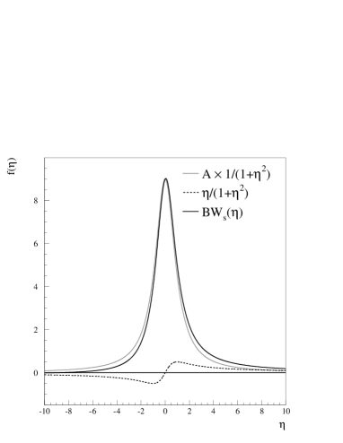
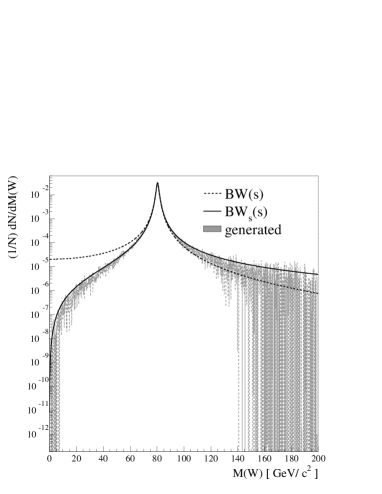
Figure 30: Left Comparisons of the two functional terms contributing to ${\rm BW}_{s}(\eta)$ given by Equation 186. Note that the scaling factor $A$ is chosen in view of making the contributions more transparent; it is much too small compared to the real case of $W^{\pm}/Z^{0}$ bosons. Right Comparison of the (normalized) distributions of differential cross-section for the process $q\bar{q}\to Wb\bar{b}$ (dashed) and sampling functions (solid line) with respect to the variables obtained by importance sampling, as described in the text.

Using the above re-sampling procedure, the whole approach remains completely unitary, i.e. no events are rejected when either there are no limits set on the value of $\eta$ or they are symmetric, $|\eta_{\rm min}|=\eta_{\rm max}$. In the contrary case, a small fraction of sampling values is rejected.

As it turns out in subsequent generator level studies, this generation procedure provides a much better agreement with the differential distributions than the usual (width independent) Breit-Wigner; an example obtained for the $q\bar{q}\to Wb\bar{b}$ process is shown in Figure 30. The evident consequence is that the unweighting efficiency is substantially improved due to the reduction of the event weights in the high $s^{*}_{W}$ region.

Modified VEGAS Algorithm

Using the multi-channel approach previously described, the total generation (unweighting) efficiency amounts to about $3-10\%$ depending on the complexity of the chosen process. In order to further improve the efficiency, a set of modified VEGAS [347] routines was used as a (pseudo-)random number generator for sampling the peaking quantities in each kinematic channel. After training all the sampling grids (of dimensions 4-7, depending on the kinematic channel), the generation efficiency increased to values of above $20\%$. The motivation for this approach is, that for unitary algorithms, only a very finite set of simple sampling functions is available, since the functions have to have simple analytic integrals for which an inverse function also exists. Consequently, the non-trivial kinematic distributions can not be adequately described by simple functions in the whole sampling domain (e.g. the $\tau$ distribution, c.f. Figure 31) and some additional smoothing might be necessary.

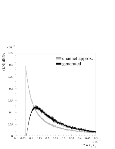
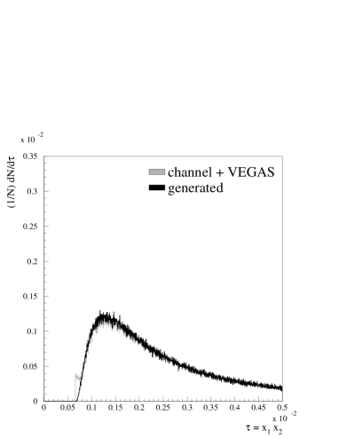
Figure 31: Comparison between the sampling distribution for the $\tau=\hat{s}/s\in[\tau_{\rm min},1]$ variable before and after the application of modified VEGAS [347] smoothing procedure (see text).

In addition, the random number distributions should, due to the applied importance sampling, have a reasonably flat behaviour to be approached by an adaptive algorithm such as VEGAS. The principal modification of VEGAS, besides adapting it to function as a (pseudo-)random number generator instead of the usual integrator, was based on the discussions [348, 349] that in the case of event generation, i.e.the unweighting of events to weight one, reducing the maximal value of event weights is in principle of higher importance than achieving the minimal weight variance. Thus, the learning algorithm was modified accordingly. By observing the distributions of the event weights before and after the inclusion of the modified ac-VEGAS algorithm (Fig. 32), it is evident that ac-VEGAS quite efficiently clusters the weights at lower values.

Figure 32: The distribution of event weights using the Multi-Channel approach only (dotted histogram) and after application of the VEGAS (dashed histogram) and ac-VEGAS (full histogram) algorithms in the $gg\to(Z^{0}\to)l\bar{l}b\bar{b}$ process.

Colour Flow Information

Before the generated events are passed to PYTHIA/HERWIG for further treatment, additional information on the colour flow/connection of the event has to be obtained. To provide an illustration, the method of the colour flow determination is described for the processes $gg\to t\bar{t}b\bar{b}$.

For the process $gg\to t\bar{t}b\bar{b}$ six colour flow configurations are possible, as shown in Figure 33. With 36 Feynman diagrams contributing to the process and at least half of them participating in two or more colour flow configurations, calculations by hand would prove to be very tedious. Consequently, a slightly modified colour matrix summation procedure from MADGRAPH [310] was used to determine the colour flow combinations of the diagrams and the corresponding colour factors. The derived squared matrix elements for the separate colour flow combinations $|{\mathcal{M}_{\rm flow}}|^{2}$ were used as sampling weights on an event-by-event basis to decide on a colour flow configuration of the event before it is passsed on to PYTHIA/HERWIG for showering and fragmentation. The procedure was verified to give identical results for the colour flow combinations and corresponding colour factors when applied to the processes published in [350].

]

Figure 33: A diagrammatic representation of the six colour flow configurations in the process $gg\to t\bar{t}b\bar{b}$.

5.3.2 How to use the package

The AcerMC 1.0 package consists of the library of the matrix-element-based generators for the selected processes, interfaces to the PYTHIA 6.2 and HERWIG 6.3 generators, and two main programs: demo_hw.f and demo_py.f. The makefiles provided allow the user to build executables with either of these generators: demo_hw.exe or demo_py.exe.

There are two steering input files: run.card and acermc.card, which have the same form for both executables. The run.card file provides switches for modifying the generated process, the number of events, the structure functions, and predefined option for hadronisation/fragmentation, random number, etc.. The acermc.card file provides switches for modifying more specialized settings for the AcerMC 1.0 library itself. Once the user decides on the setup for the generated process, only the run.card very likely needs to be modified for the job submission.

The same executables can be also used for generating standard PYTHIA 6.2/HERWIG 6.3 processes. Examples of how to run such jobs are provided as well, in respectively demo_hw.f and demo_py.f. If the user requires that the AcerMC library is not used, $ttH$ production will be generated with demo_py.exe, and the HERWIG 6.3 implementation of the $Zbb$ production will be generated with demo_hw.exe. Only in this case will the run.card file be read, so the user should implemente her/his steering there or create another xxx.card file, and add the respective code to the demo_xx.f.

The AcerMC 1.0 matrix-element-based generators are very highly optimized, using multi-channel optimization and additional improvement with the VEGAS grid. The generation modules require three kinds of the input data to perform the generation of unweighted events: (1) A file containing the list of the values of relative channel weights obtained by the multi-channel optimization. (2) A file containing the pre-trained VEGAS grid. (3) A file containing the maximum weight $wt_{\rm max}$, $\epsilon$-cutoff maximum weight $wt_{\rm max}^{\epsilon}$ and the 100 events with the highest weights. This means that in the case of changing the default running conditions, such as the structure functions or centre-of-mass energy, in order to recover the initial efficiency for event generation, the user should repeat the process of preparation of the internal data files with the inputs for the phase-space generator modules. Pre-trained data sets obtained using $\sqrt{s}=14\;$ TeV, PYTHIA default $\alpha_{s}(Q^{2})$ and $\alpha_{\rm QED}(Q^{2})$ and the CTEQ5L (parametrized) structure function set are already provided for each implemented process.

The number of required input files might at first glance seem large, considering that many event generators do not require any input files for operation; the difference is not so much in the complexity of the phase space generation as in the fact that many event generators require a warming run instead. That is, before the generation of unweighted events is performed a certain number of weighted events (typically of the order of $10^{4}$) is generated in order to obtain the relative multi-channel weights (in case multi-channel phase space generation is used) and/or the optimized VEGAS grid and/or an estimate of the maximal weight. Such an approach can have an advantage when event generation is very fast and the phase space regions with the highest weights are well known (as done for the $2\to 2$ processes in PYTHIA); on the other hand, when the phase space topology of the process is more complex and the event generation is comparatively slow, generating a relatively small number of e.g. $10^{4}$ weighted events every time a generator is started can become CPU wasteful and/or inaccurate in terms of maximum weight estimation.

Reasonably accurate estimation of the latter is mostly crucial for correct event unweighting; event generators using the warming-up method for maximal weight search often find still higher weights during the normal run and reset the maximal weight accordingly. In this case however, the statistically correct approach would be to reject all events generated beforehand and start the event generation anew. This is almost never implemented due to the CPU consumption and the possibility of hitting a weak singularity. With a small pre-sampled set the generator can, however, badly under-estimate the maximum weight and a large number of events can be accepted with a too-high probability. The only hope of obtaining correct results in such cases is that the weight plateau will be hit sufficiently early in the event generation process. Consequently, such an approach can be very dangerous when generating small numbers of events.

In contrast to the warming-up approach, we have decided that using separate training runs with large numbers of weighted events to obtain the optimized grids and maximum weight estimates is preferable. In case the user wants to produce data sets for non-default settings, this can easily be done by configuring the switches in the acermc.card

5.3.3 Outlook and conclusions

We have presented here the AcerMC 1.0 Monte Carlo Event Generator,which is based on a library of matrix-element-based generators and an interface to the universal event generator PYTHIA 6.2 and HERWIG 6.3. The interface is based on the standard proposed in section 5.2.

The presented library fulfils following goals:

• It provides a possibility to generate a few Standard Model background processes which were recognised as being very dangerous for searches for New Physics at LHC, and for which generation was either unavailable or not straightforward thus far.

• Although the hard process event is generated with a matrix-element-based generator, the provided interface allows a complete event to be generated with either PYTHIA 6.2 or HERWIG 6.3 initial and final state radiation, multiple interaction, hadronization, fragmentation and decays.

• The interface can be also used for studying systematic differences between PYTHIA 6.2 or HERWIG 6.3 predictions for the underlying QCD processes.

These complete the list of the native AcerMC processes implemented so far is: $q\bar{q}\to W(\to\ell\nu)b\bar{b}$, $gg,q\bar{q}\to Z/\gamma^{*}(\to\ell\ell)b\bar{b}$, QCD $gg,q\bar{q}\to t\bar{t}b\bar{b}$ and EW $gg\to(Z/W/\gamma^{*}\to)t\bar{t}b\bar{b}$, $q\bar{q}\to W(\to\ell\nu)t\bar{t}$ and $gg,q\bar{q}\to Z/\gamma^{*}(\to\ell\ell,\nu\nu,b\bar{b})t\bar{t}$. We plan to extend this crucial list of processes, gradually in the near future.

5.4 Comparisons of Higgs Boson Properties with Soft Gluon Emission: Analytic and Parton Showering Methods

In the near future, experiments at the Tevatron and the LHC will search for evidence of both the Higgs boson and new phenomena that supersede the Standard Model. Important among the tools that will be used in these searches are event generators based on parton showering (PS-EG’s). The most versatile and popular of these are the Monte Carlos HERWIG [309, 339, 340, 236], ISAJET [311], and PYTHIA [313, 317]. PS-EG’s are useful because they accurately describe the emission of multiple soft gluons (which is, in effect, an all orders problem in QCD) and also allow a direct connection with non–perturbative models of hadronization. In the parton shower, energy–momentum is conserved at every step, and realistic predictions can be made for arbitrary physical quantities. However, the prediction of the total cross section is only accurate to leading order accuracy, and, thus, can demonstrate a sizable dependence on the choice of scale used for the parton distribution functions (PDF’s) or coupling constants (particularly $\alpha_{s}$). Also, in general, they do not accurately describe kinematic configurations where a hard parton is emitted at a large angle with respect to other partons. In distinction to PS-EG’s are certain analytic calculations which account for multiple soft gluon emission and higher order corrections to the hard scattering simultaneously using resummation. The resummation technique systematically includes towers of logarithms which are formally of the same order using the renormalization group. These calculations, however, integrate over the kinematics of the soft gluons, and, thus, are limited in their predictive power. They can, for example, describe the kinematics of a heavy gauge boson produced in hadron collision, but cannot predict the number or distribution of jets that accompany it.

Much recent work has focused on correcting the parton shower predictions to reproduce the hard emission limit, where the exact leading order matrix element gives an accurate description, with work proceeding on extending this correction to next-to-leading order [351, 352, 353, 354]. In order to match this precision, it is also important to verify that the PS-EG programs correctly reproduce the expected logarithmic structure in their simulation of multiple, soft gluon emission. The best approximation we have of the expected logarithmic structure is represented by resummation calculations.

Since Standard Model Higgs boson production is a primary focus of the physics program at the Tevatron and the LHC, and since several PS-EG and analytic resummation predictions exist, we have chosen $gg\to H$ production as a benchmark for evaluating the consistency and accuracy of these two approaches. In particular, the transverse momentum of the Higgs boson $Q_{T}^{H}$ depends primarily on the details of the soft gluon emission from the initial state partons. The $gg$ initial state is particularly interesting, since the large color charge may emphasize any differences that might exist in parton shower/resummation implementations. Furthermore, for the $gg$ induced process, the details of non–perturbative physics (e.g. intrinsic $k_{T}$) are less important [171, 276].

To this end, we have compared Higgs production using HERWIG, PYTHIA (several recent versions) and ResBos [179] for Higgs masses of 125 and 500 GeV at center-of-mass energies of 1.96 TeV (${{\rm p}\bar{\rm p}}$), 14 and 40 TeV (${\rm pp}$). The two different masses and three different center of mass energies provide a wide variation of kinematics that test the showering/resummation processes. This work extends our results published in [355, 276], [356] and [171].

5.4.1 Parton Showers

PS-EG’s are based on the factorization theorem [357], which, roughly, states that physical observables in any sensible gauge theory are the product of short–distance functions and long–distance functions. The short–distance functions are calculable in perturbation theory. The long–distance functions are fit at a scale, but their evolution to any other scale is also calculable in perturbation theory.

A standard application of the factorization theorem is to describe heavy boson production at a hadron collider to a fixed order in $\alpha_{s}$. The production cross section is obtained by convoluting the partonic subprocesses evaluated at the scale $Q$ with the PDF’s evaluated at $Q$. The partons involved in the hard collision must be sufficiently virtual to be resolved inside the proton, and a natural choice for the scale $Q$ is the mass of the heavy boson [358]. Prior to the hard collision, however, the partons are not resolvable in the proton (i.e. the proton is intact) and have virtualities at a much lower scale $Q_{0}$ of the order of 1 GeV. The connection between the partons at the low scale $Q_{0}$ and those at the high scale $Q$ is described by the DGLAP evolution equations [359, 264, 360]. The DGLAP equations include the most important kinematic configurations of the splittings $a\to bc$, where $a,b$ and $c$ represent different types of partons in the hadron ($q,g$, etc.). Starting from a measurement of the PDF’s at a low scale $Q_{0}$, a solution of the DGLAP equations yields the PDF’s at the hard scale $Q$. Equivalently, starting with a parton $c$ involved in a hard collision, it is also possible to determine probabilistically which splittings generated $c$. In the process of de–evolving parton $c$ back to the valence quarks in the proton, a number of spectator partons (e.g. parton $b$ in the branching $a\to bc$) are resolved. These partons constitute a shower of soft jets that accompany the heavy boson, and influence its kinematics.

The shower described above occurs with unit probability and does not change the total cross section for heavy boson production calculated at the scale $Q$ [361]. The showering can be attached to the hard–scattering process based on a probability distribution after the hard scattering has been selected. Once kinematic cuts are applied, the transverse momentum and rapidity of the heavy boson populate regions never accessed by the differential partonic cross section calculated at a fixed order. This is consistent, since the fixed–order calculation was inclusive and was never intended to describe the detailed kinematics of the heavy boson. The parton shower, in effect, resolves the structure of the inclusive state of partons denoted as $X$. In practice, the fixed order partonic cross section (without showering) can still be used to describe properties of the decay leptons as long as the measurable is not highly correlated with the heavy boson kinematics.

Here, we review parton showering schematically. More details can be found, for example, in Ref. [362]. First, for simplicity, consider the case of final state or forward showering, where the parton virtuality $Q$ evolves forward to the low scale $Q_{0}$. The basis for developing a probabilistic picture of final state showering is the DGLAP equation for the fragmentation functions:

$$Q{\partial\over\partial Q}D_{a}(x,Q)=\int_{x}^{1-\epsilon}{dz\over z}{\alpha_{abc}(z,Q)\over\pi}\hat{P}_{a\to bc}(z)D_{b}(x/z,Q)$$

$$-D_{a}(x,Q)\int_{x}^{1-\epsilon}{dz}{\alpha_{abc}(z,Q)\over\pi}\hat{P}_{a\to bc}(z),$$ (190)

where $\hat{P}_{a\to bc}$ is an unregularized splitting function, $\alpha_{abc}$ is the coupling times color factor, and $\epsilon$ is a cutoff. The equation can be rewritten as

$${\partial\over\partial\ln Q^{2}}\left(D_{a}(x,Q)/\Delta(Q)\right)=\int_{x}^{1}{dz\over z}{\alpha_{abc}(z,Q)\over 2\pi}\hat{P}_{a\to bc}(z)(D_{b}(x/z,Q)/\Delta(Q))$$

or, after integrating both sides of the expression,

$$D_{a}(x,t^{\prime})=D_{a}(x,t)\Delta(t^{\prime})+\int_{t^{\prime}}^{t}\int_{x}^{1}dt^{\prime\prime}{dz\over z}{\Delta(t^{\prime})\over\Delta(t^{\prime\prime})}{\alpha_{abc}(z,t^{\prime\prime})\over 2\pi}\hat{P}_{a\to bc}(z)D_{b}(x/z,t^{\prime\prime}),$$ (191)

where $t=\ln Q^{2},$ with similar definitions for $t^{\prime}$ and $t^{\prime\prime}$. The function

$$\Delta(t^{\prime})=\exp\left(-\int_{t_{0}}^{t^{\prime}}\int_{\epsilon}^{1-\epsilon}dt^{\prime\prime}dz{\alpha_{abc}(z,t^{\prime\prime})\over 2\pi}\hat{P}_{a\to bc}(z)\right)$$ (192)

is called the Sudakov form factor, and gives the probability of evolving from the scale $t^{\prime}$ to $t_{0}$ with no resolvable branchings, where $t_{0}$ is a cutoff scale for the showering. The Sudakov $\Delta(t^{\prime})$ contains all the information necessary to reconstruct a shower, since it encodes the change in virtuality of a parton until a resolvable showering occurs. Showering is reduced to iterative solutions of the equation $r=\Delta(t^{\prime})/\Delta(t^{\prime\prime})$, where $r$ is a random number uniformly distributed in the interval $[0,1]$, until a solution for $t^{\prime}$ is found which is below the cutoff $t_{0}$.

For the case of initial state radiation, several modifications are necessary. The fragmentation function is replaced by a parton distribution function, and the evolution proceeds backwards from a large, negative scale $-|Q^{2}|$ to a small, negative cutoff scale $-|Q_{0}^{2}|$. There are two equivalent formulations of backwards showering based on the probabilities

$$\exp\left(-\int_{t^{\prime}}^{t}\int_{\epsilon}^{1-\epsilon}dt^{\prime\prime}dz{\alpha_{abc}(z,t^{\prime\prime})\over 2\pi}\hat{P}_{a\to bc}(z){x^{\prime}f_{a}(x^{\prime},t^{\prime})\over xf_{b}(x,t^{\prime})}\right),x^{\prime}=x/z,$$ (193)

[363], and

$${\Delta(t^{\prime})\over f_{b}(x,t^{\prime})}{f_{a}(x,t^{\prime\prime})\over\Delta(t^{\prime\prime})}$$ (194)

[364]. After choosing the change in virtuality, a particular backwards branching is selected from the probability function based on their relative weights (a summation over all possible branchings $a\to bc$ is implied these expressions), and the splitting variable is a solution to the equation

$$\int_{\epsilon}^{x/x^{\prime}}{dz\over z}\hat{P}_{a\to bc}(z)f(x/z,t^{\prime})=r\int_{\epsilon}^{1-\epsilon}{dz\over z}\hat{P}_{a\to bc}(z)f(x/z,t^{\prime}),$$ (195)

where $r$ is a random number. The details of how a full shower is reconstructed in PYTHIA, for example, can be found in Ref. [295]. The structure of the shower can be complex: the transverse momentum of the heavy boson is built up from the whole series of splittings and boosts, and is known only at the end of the shower, after the final boost.

The PS-EG formulation outlined above is fairly independent of the hard scattering process considered. Only the initial choice of partons and possibly the high scale differs. Therefore, this formalism can be applied universally to many different scattering problems. In effect, soft gluons are not sensitive to the specifics of the hard scattering, only the color charge of the incoming partons. This statement is true to leading logarithm.

The parton showering of PYTHIA obeys a strict ordering in virtuality: the parton that initiates a hard scattering has a larger (negative for initial state showers) virtuality than any other parton in the shower. Parton showers in HERWIG proceed via a coherent branching process in which a strict angular ordering is imposed on sequential gluon emissions: the evolution variable is not virtuality, but a generalized virtuality $\xi$. For an initial state shower, with parton splitting $c\to ba$, and where $a$ has the largest virtuality, the variable $\xi=(p_{b}\cdot p_{c})/(E_{b}E_{c})$. At all values of $x$, the coherent branching algorithm correctly sums the leading logarithmic contributions. At large $x\sim 1$, it also sums the next-to-leading order contributions [236], with an appropriate definition of the splitting kernel. (The exact definition of LL and NLL will be given later.) Because of the demonstrated importance of coherence effects, PYTHIA includes an additional veto on showers which are not also angular–ordered. Note, however, that this does not make the two schemes equivalent – some late emissions in a HERWIG shower can have virtuality larger than previous emissions.

5.4.2 Analytic results

At hadron colliders, the partonic cross sections for heavy boson production can receive substantial corrections at higher orders in $\alpha_{s}$. This affects not only the total production rate, but also the kinematics of the heavy boson. At leading order, the heavy boson has a $\delta(Q_{T}^{2})$ distribution in $Q_{T}^{2}$. At next–to–leading order, the real emission of a single gluon generates a contribution to $d\sigma/dQ_{T}^{2}$ that behaves as $Q_{T}^{-2}\alpha_{s}(Q_{T}^{2})$ and $Q_{T}^{-2}\alpha_{s}(Q_{T}^{2})\ln(Q^{2}/Q_{T}^{2})$ while the soft, and virtual corrections are proportional to $-\delta(Q_{T}^{2})$. At higher orders, the most singular terms follow the pattern of $\alpha_{s}^{n}(Q_{T}^{2})\sum_{m=0}^{2n-1}\ln^{m}(Q^{2}/Q_{T}^{2})$ $=\alpha_{s}^{n}L\equiv V^{n}$. The logarithms arise from the incomplete cancellation of the virtual and real QCD corrections. This cancellation becomes complete for the integrated spectrum, where the real gluon can become arbitrarily soft and/or collinear to other partons. The pattern of singular terms suggest that perturbation theory should be performed in powers of $V^{n}$ instead of $\alpha_{s}^{n}$. This reorganization of the perturbative series is called resummation.

The first studies of soft gluon emission resummed the leading logarithms [365, 366], leading to a suppression of the cross section at small $Q_{T}$. The suppression underlines the importance of including sub–leading logarithms [367]. The most rigorous approach to the problem of multiple gluon emission is the Collins–Soper–Sterman (CSS) formalism for transverse momentum resummation [368], which resums all of the important logarithms. This is achieved after a Fourier transformation with respect to $Q_{T}$ in the transverse coordinate $b$, so that the series involving the delta function and terms $V^{n}$ simplifies to the form of an exponential. Hence, the soft gluon emission is resummed or exponentiated in this $b$–space formalism. The Fourier transformation is the result of expressing the transverse–momentum conserving delta functions $\delta^{(2)}(\vec{Q}_{T}-\sum\vec{k}_{T_{i}})$ in their Fourier representation. Also, the exponentiation is accomplished through the application of the renormalization group equation. Despite the successes of the $b$–space formalism, there are several drawbacks. Most notable for the present study is that it integrates out the soft gluon dynamics and does not have a simple physical interpretation.

The CSS formalism was used by its authors to predict both the total cross section to NLO and the kinematic distributions of the heavy boson to resummed NLL order [174] at hadron colliders. A similar treatment was presented using the AEGM formalism [369], that does not involve a Fourier transform, but is evaluated directly in transverse momentum $Q_{T}$ space. When expanded in $\alpha_{s}$, the two formalisms are equivalent to the NNNL order, and agree with the NLO fixed order calculation of the total cross section [370]. A more detailed numerical comparison of the two predictions can be found in Ref. [371]. The AEGM formalism has been reinvestigated, and an approximation to the $b$–space formalism has been developed in $Q_{T}$–space which retains much of its predictive features [372].

In the $b$–space formalism, the differential cross section of the heavy boson produced in association with soft gluons is:

$${d\sigma(h_{1}h_{2}\to B^{(*)}X)\over dQ^{2}\,dQ^{2}_{T}\,dy}={1\over(2\pi)^{2}}\int d^{2}b\,e^{i{\vec{b}}\cdot{\vec{Q}_{T}}}\widetilde{W}(b,Q,x_{1},x_{2})+Y(Q_{T},Q,x_{1},x_{2}).$$ (196)

where $Q$, $Q_{T}$ and $y$ describe the kinematics of the off–shell heavy boson $B^{(*)}$. The function $Y$ is free of $\ln(Q^{2}/Q_{T}^{2})$ and corrects for the soft gluon approximation in the high $Q_{T}$ region. The function $\widetilde{W}$ has the form:

$${\widetilde{W}}(b,Q,x_{1},x_{2})=e^{-S(b,Q)}\left(C_{il}\otimes f_{l/h_{1}}\right)(x_{1},b)\left(C_{jl}\otimes f_{l/h_{2}}\right)(x_{2},b)H_{ij}(Q,y),$$ (197)

where

$$S(b,Q,C_{1},C_{2})=\int_{C_{1}^{2}/b^{2}}^{C_{2}^{2}Q^{2}}{d{\bar{\mu}}^{2}\over{\bar{\mu}}^{2}}\left[\ln\left({C_{2}^{2}Q^{2}\over{\bar{\mu}}^{2}}\right)A\big{(}\alpha_{s}({\bar{\mu}})\big{)}+B\big{(}\alpha_{s}({\bar{\mu}})\big{)}\right],$$ (198)

and

$$\left(C_{jl}\otimes f_{l/h_{1}}\right)(x_{1},\mu)=\int_{x_{1}}^{1}{d\xi_{1}\over\xi_{1}}\,C_{jl}\left({x_{1}\over\xi_{1}},C_{1},C_{2},\mu=C_{3}/b\right)f_{l/h_{1}}\left(\xi_{1},\mu=C_{3}/b\right).$$ (199)

In these expressions, $C_{1}$, $C_{2}$ and $C_{3}$ are renormalization scales, $H$ is a function that describes the hard scattering, and $A$, $B$ and $C$ are calculated perturbatively in powers of $\alpha_{s}$:

$$\{A,B\}=\sum_{n=1}^{\infty}\left({\alpha_{s}(\mu)\over\pi}\right)^{n}\{A^{(n)},B^{(n)}\}~{}~{}~{}{\rm and}~{}~{}~{}C_{ij}=\sum_{n=0}^{\infty}\left({\alpha_{s}(\mu)\over\pi}\right)^{n}C^{(n)}.$$

The functions $C^{(n)}$ are mostly responsible for the change in the total production cross section at higher orders. In fact, $\left(C\otimes f\right)$ is simply a redefinition of the parton distribution function obtained by convoluting the standard ones with an ultraviolet–safe function. These generalized parton distributions encode both the longitudinal momentum fraction and the transverse recoil of the initial state parton.

We remove $C_{1},C_{2}$ and $C_{3}$ from these expressions by choosing their canonical values [368], which also removes large logarithms from the expansion of the resummed expression. At leading order in $C_{ij}$, the resummed part of the expression for the production of an on–shell heavy boson simplifies considerably to:

$${d\sigma(h_{1}h_{2}\to B^{(*)}X)\over dQ^{2}_{T}}=\sigma_{0}\int{d^{2}b\over(2\pi)^{2}}\,e^{i{\vec{b}}\cdot{\vec{Q}_{T}}}e^{-S(b,Q)}{f(x_{1},b)f(x_{2},b)\over f(x_{1},Q)f(x_{2},Q)},$$ (200)

where

$$\sigma_{0}=\kappa\int{dx_{1}\over x_{1}}f(x_{1},Q)f(x_{2},Q),$$

and $\kappa$ contains physical constants. The expression contains two factors, the total cross section at leading order $\sigma_{0}$, and a cumulative probability function in $Q_{T}^{2}$ that describes the transverse momentum of the heavy boson (the total integral over $Q_{T}^{2}$ transforms $e^{i\vec{b}\cdot\vec{Q}_{T}}$ to $\delta^{(2)}(\vec{b})$). Except for the complication of the Fourier transform, the term $e^{-S/2}f(x,b)/f(x,Q)$ is analogous to $\Delta(Q)f(x,Q^{\prime})/\Delta(Q^{\prime})f(x,Q)$ of the PS-EG of Eq. (194).

Equation (196), which is formulated in $b$–space, has a similar structure in $Q_{T}$–space. This is surprising, since the $b$–space result depends critically on the conservation of total transverse momentum. To NNNL accuracy, however, the $Q_{T}$ space expression agrees exactly with the $b$–space expression, and has the form [372]:

$${d\sigma(h_{1}h_{2}\to B^{(*)}X)\over dQ^{2}\,dQ^{2}_{T}\,dy}={d\over dQ_{T}^{2}}\widetilde{W}(Q_{T},Q,x_{1},x_{2})+Y(Q_{T},Q,x_{1},x_{2}).$$ (201)

Again ignoring $Y$, we can rewrite this expression as:

$${d\sigma(h_{1}h_{2}\to B^{(*)}X)\over dQ_{T}^{2}}=\sigma_{1}\left({d\over dQ_{T}^{2}}\left[e^{-S(Q_{T},Q)}{\left(C\otimes f\right)(x_{1},Q_{T})\left(C\otimes f\right)(x_{2},Q_{T})\over\left(C\otimes f\right)(x_{1},Q)\left(C\otimes f\right)(x_{2},Q)}\right]\right),$$ (202)

$$\sigma_{1}=\kappa\int{dx_{1}\over x_{1}}\left(C\otimes f\right)(x_{1},Q)\left(C\otimes f\right)(x_{2},Q).$$

The factor $\sigma_{1}$ is the total cross section to a fixed order, while the rest of the function yields the probability that the heavy boson has a transverse momentum $Q_{T}$.

5.4.3 Methodology for comparison

To make a comparison between the distributions from analytic and parton showering calculations, we must quantify the differences in theoretical input and identify what approximations have been made in each one. ¿From the discussion of the analytic resummation calculations, we see that the emission of multiple soft gluons is described best by perturbation theory not in terms of $\alpha_{s}$, but in powers of $\alpha_{s}$ times logarithms of large numbers. Typically, the logarithms are classified according to the orders of $\alpha_{s}$ and the power of logarithms in $(i)$ the Sudakov exponent, or in $(ii)$ the perturbative expansion of the resummed $Q_{T}$ distribution.

In classification $(i)$, it is argued that terms with $A^{(n)}$ are leading compared to terms with $B^{(n)}$ because the former are enhanced by a large logarithm. Also, $X^{(n)}$ is leading compared to $X^{(n+1)}$ because the latter is suppressed by $\alpha_{s}$ for $X=A,B$ or $C$. The comparison of $C$ to $A$ and $B$ is somewhat ad hoc, because $C$ does not appear in the Sudakov in all resummation schemes. In this approach, the lowest order resummed result (LL) has only $A^{(1)}$ and $C^{(0)}$. Additionally, the next order (NLL) has $A^{(2)}$, $B^{(1)}$ and $C^{(0)}$, because the first two are suppressed by an $\alpha_{s}$ and the last by the inverse of a large logarithm when compared to the leading terms. This is an elegant and simple classification scheme, because it relies only on the structure of the Sudakov exponent. On the other hand, it has an ad hoc mixing $\alpha_{s}$ and $\log^{-1}$–suppressed terms, and depends on the resummation scheme in dealing with $C^{(n)}$.

In classification $(ii)$, the resummed cross section is expanded and reorganized in towers of logarithms as

$$\frac{d\sigma}{dQ_{T}^{2}}\sim\begin{array}[]{llll}\alpha_{s}^{1}(L_{1}^{1})&+&&\\ \alpha_{s}^{2}(L_{2}^{1}&+L_{2}^{3})&+&\\ \alpha_{s}^{3}(L_{3}^{1}&+L_{3}^{3}&+L_{3}^{5})&+\cdots,\end{array}$$ (206)

where $L_{i}$ are various linear combinations of $\ln(Q/Q_{T})$. Remarkably, each column of logs receives contribution only from $A^{(n)}$, $B^{(n)}$ and $C^{(n-1)}$ ($n$ numbers the columns). Since $X^{(n)}$ and $X^{(n+1)}$ are clearly ordered by $\alpha_{s}$ ($X=A,B,C$), the first column is called the leading tower of logs, i.e. LL, the next NLL, etc. This is a more–involved classification, but closer to the spirit of the resummation, and more precise. In the rest of this work, we use the naming convention $(ii)$ when comparing to the analytic resummation. Thus, when we say that the coherent branching algorithm in HERWIG correctly sums the leading logarithmic contributions, we are referring to the $A^{(1)}$ and $B^{(1)}$ terms.

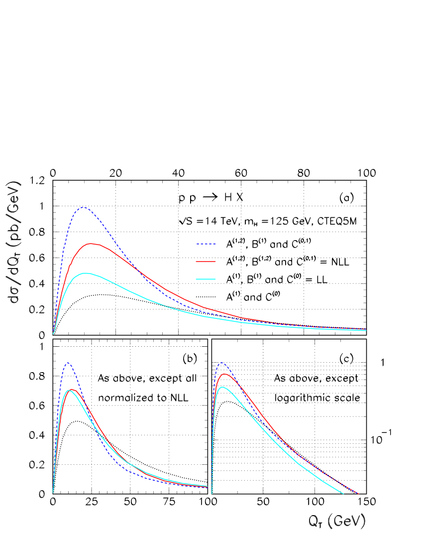
Figure 34: (top) Absolute $Q_{T}$ distribution of the Higgs boson from an analytic resummation calculation to different orders of accuracy in perturbation theory; (left, bottom) Same as (top), but normalized to the same total cross section; (right, bottom) Same as (left,bottom), but on a logarithmic scale. All curves are for the production of a 125 GeV Higgs boson at the LHC based on the CTEQ4M parton distribution functions.

Figure 34 demonstrates the different predictions for different choices of organizing the perturbative expansion. The top frame shows the absolute distributions of $Q_{T}^{H}$ when the perturbative coefficients include: $A^{(1,2)},~{}B^{(1,2)},~{}C^{(0,1)}$ (solid red), $A^{(1,2)},~{}B^{(1)}$ and $C^{(0,1)}$ (long-dashed blue), $A^{(1)},~{}B^{(1)}$ and $C^{(0)}$ (solid light blue), and only $A^{(1)}$ and $C^{(0)}$ (short-dashed black). The change from LL to NLL results in an increase of the normalization of the cross section as well as a slight shift of the peak towards higher transverse momentum, but the shapes are very similar. The lower left frame shows the same distributions, but all normalized to the same production rate. This eliminates the normalization dependence and focuses on the variation of the shape. The lower right frame, shown in logarithmic scale, amplifies the differences at high $Q_{T}$’s.

5.4.4 Numerical comparisons

In the following plots, we show several numerical comparisons of ResBos, HERWIG and three versions of PYTHIA. Why three versions of PYTHIA? This reflects the evolution of the program. The version PYTHIA-5.7 was used for almost all LHC Monte Carlo analyses for Higgs production. The showering in PYTHIA-5.7, as described earlier, is virtuality ordered, with an additional requirement of angular ordering. No other kinematic restrictions are imposed. In later versions, beginning with PYTHIA-6, each parton emission was required to match the kinematic constraints of the NLO process, i.e. for the first emission in the parton shower accompanying $gg\to H$, the kinematic constraints $\hat{s}+\hat{t}+\hat{u}=M_{H}^{2}$ must be satisfied. Since $\hat{s}$ and $\hat{t}$ are the two variables of the virtuality–ordered shower, a cut on $\hat{u}$ restricts their range. The plots labeled by PYTHIA6.1 demonstrate the effect of the $\hat{u}$ cut. Finally, in PYTHIA-6.2, an additional hard matrix element correction was applied to the parton shower. In this approach, the maximum virtuality of the shower is increased from its nominal value at $Q=m_{H}$ up to the largest kinematically allowed value. Furthermore, each parton emission is corrected by the ratio of the exact matrix element squared at NLO to the approximate matrix element squared given by the parton shower approximation. Thus, showers generated using PYTHIA-6.2 should have a closer agreement to the ResBos predictions at high $Q_{T}^{H}$ (where ResBos relies on the NLO prediction). In contrast, showers induced in HERWIG will still have a cutoff set by $m_{H}$. Note, however, that the PYTHIA prediction still has the LO normalization, and a full rescaling is necessary. This may be appropriate if the $K$–factor correction to the LO prediction is the same as the one for the NLO emission.

Figures 35 and 36 show the predicted $Q_{T}$ distributions for production of a Standard Model Higgs boson with mass $m_{H}=125$ GeV at collider energies of 1.96, and 14 TeV. For all plots, the distributions have been normalized to the same cross section (ResBos NLL); without this normalization, the PS-EG predictions would be about a factor of 2 lower than the ResBos curves. Two ResBos curves are shown: LL (including $A^{(1)}$, $B^{(1)}$ and $C^{(0)}$) and NLL (also including $A^{(2)}$, $B^{(2)}$ and $C^{(1)}$ ). The inclusion of the NLL terms leads to a slightly harder $Q_{T}$ distribution, as discussed previously. The ResBos curves appear close to the HERWIG predictions, and somewhat less close to the predictions of PYTHIA (versions 6.1 and after).

In general, the PS-EG predictions are in fair agreement with the analytic resummation ones for low $Q_{T}$, where multiple, soft gluon emission is the most important. The agreement of HERWIG with the ResBos curves becomes even better if the shape comparison are made by normalizing the cross sections in the low $Q_{T}$ region alone, away from the effects of the exact matrix element for Higgs plus jet. This is illustrated in Figures 36. The PYTHIA-6+ predictions peak at a noticeably lower value of $Q_{T}$ than either ResBos or HERWIG. A striking feature of the plots is the change induced in PYTHIA-6.1 relative to PYTHIA-5.7, indicating the importance of kinematic constraints. Note also that the average Higgs transverse momentum increases with increasing center-of-mass energy, due to the increasing phase space available for gluon emission. At high $Q_{T}$, the exact matrix element for Higgs plus jet, present both in the most recent version of PYTHIA as well as ResBos, correctly describes Higgs production at transverse momenta on the order of the Higgs mass or larger, while a pure parton showering description of the high $Q_{T}$ end is inadequate. The change observed in 6.2, only visible at large values of $Q_{T}$, is the result of the matrix element (Higgs + jet) corrections to the parton shower.

The final comparison plot, Figure 37, shows the $Q_{T}$ distributions for a 500 GeV Higgs boson generated through $gg$ fusion at 14 TeV (pp) and 40 TeV (pp). Comparisons are made of the ResBos(LL and NLL), PYTHIA and HERWIG predictions. As in Figures 35 and 36 the distributions have been scaled to have the same total cross section. The average transverse momentum for a 500 GeV Higgs is noticeably larger than that for a 125 GeV Higgs in all of the predictions, as expected, since the hard scale for the process is $m_{H}$. The agreement between the HERWIG (version 6.1 and later) predictions and the ResBos curves is better than for the predictions with a 125 GeV mass Higgs. The agreement between HERWIG and the ResBos curves remains very good. For high $Q_{T}$, the PYTHIA 6.2 prediction, with matrix element corrections, agrees with the ResBos prediction.

Figure 35: Transverse momentum $Q_{T}$ distributions of a 125 GeV Higgs boson produced at the Tevatron for HERWIG, different versions of PYTHIA and different perturbative orders of ResBos. The bottom plot is for an expanded $Q_{T}$ range. All curves are normalized to the same total cross section.

Figure 36: Comparison of light Higgs boson production at the LHC. The right hand plots have PYTHIA 5.7, 6.1 and HERWIG distributions normalized to 90% of the ResBos NLL cross section.

Figure 37: Comparison of Higgs boson production at the LHC and 40 TeV $m_{H}=500$ GeV.

5.4.5 Properties of showers

In the previous section, there were notable differences in the predictions of PYTHIA and HERWIG, with HERWIG giving a superior description of the Higgs boson properties for low $Q_{T}^{H}$. Therefore, we have investigated several basic properties of the parton emissions to determine the cause of this discrepancy. It is already known that the HERWIG shower is of the coherent kind, whereas PYTHIA is virtuality ordered with approximate angular ordering superimposed. On the other hand, the same was true in PYTHIA5.7, but closer agreement with HERWIG is obtained after making the $\hat{u}$ cut. Perhaps a more careful analysis of the HERWIG kinematics will result in even better agreement.

Figure 38 shows a comparison of showering properties for light Higgs boson production at the Tevatron. For the purpose of these plots, the matrix element corrections in PYTHIA have been turned off. The leftmost plot shows the transverse momentum of the Higgs boson and the first parton emission for PYTHIA (red) and HERWIG (green). Note that the leading emission describes the Higgs boson $Q_{T}$ from the full shower very well down to fairly low values $\sim 10$ GeV. The main discrepancy between PYTHIA and HERWIG occurs in the same kinematic region, exactly where the properties of several emissions become important.

The rightmost plot shows the largest (negative) virtuality of a parton in the shower. The blue curve shows the effect of having no $\hat{u}$ cut, as in the older version of PYTHIA. Clearly, PYTHIA without the $\hat{u}$ cut does not have the $Q^{-2}$ behavior expected from the derivative of the Sudakov. While the agreement between PYTHIA-6.2 and HERWIG is markedly improved, PYTHIA still has a residual enhancement near the upper scale $Q=m_{H}$ in this example. This requires further investigation.

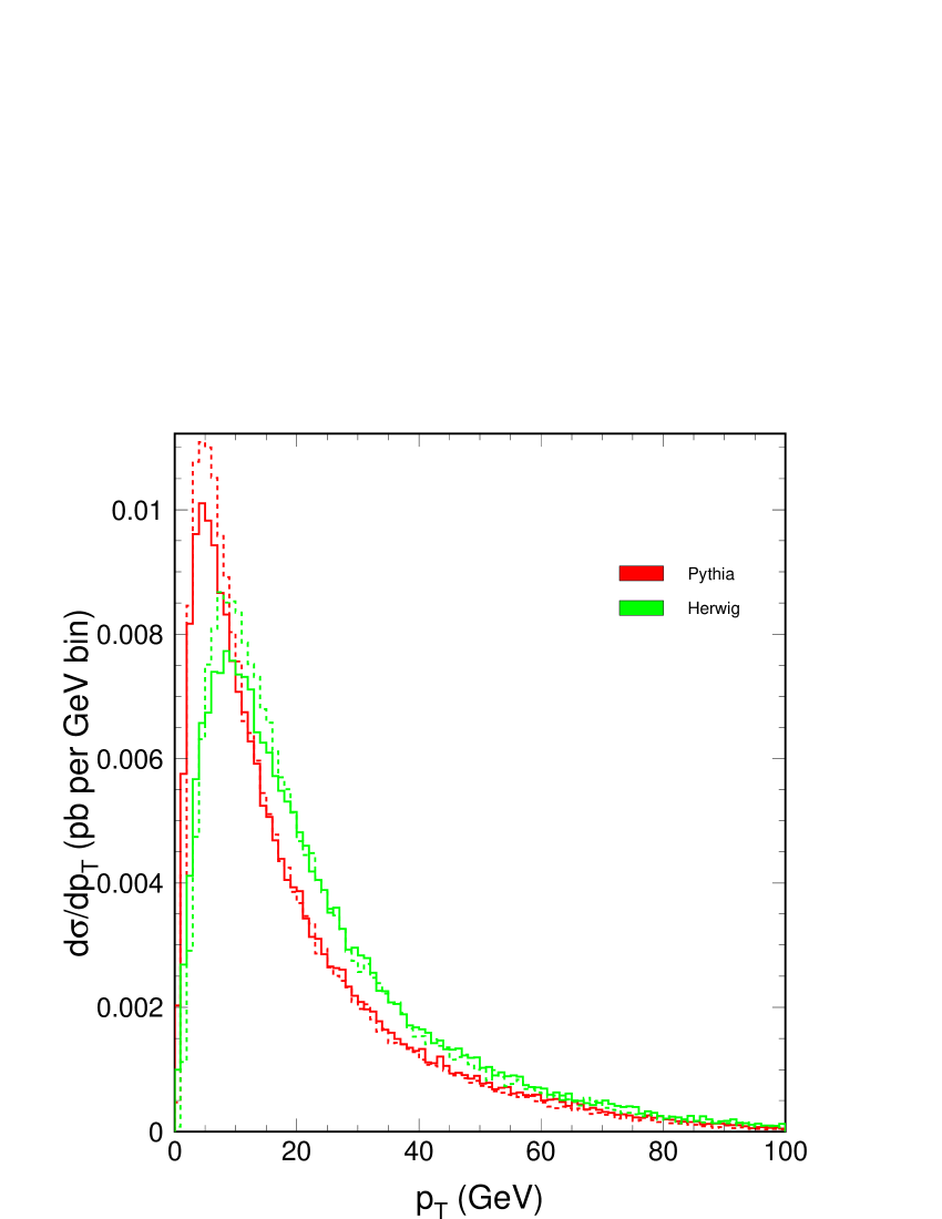
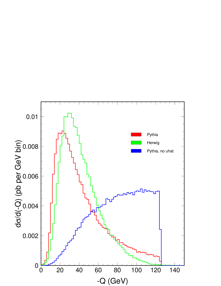
Figure 38: Comparison of showering properties for light Higgs boson production at the Tevatron. The leftmost plot shows the transverse momentum of the Higgs boson and the first parton emission for PYTHIA (red) and HERWIG (green). The rightmost plot shows the largest (negative) virtuality of parton in the shower. The blue curve shows the effect of having no $\hat{u}$ cut.

To summarize:-

• The differences between ResBos LL and NLL are in the direction expected and are relatively subtle.

• The two newer versions of PYTHIA and HERWIG both approximately agree with the predictions of ResBos LL/NLL, with the HERWIG shape agreement being somewhat better in the low $Q_{T}$ region.

• The agreement of HERWIG with ResBos becomes better as: $(a)$ the center of mass energy increases and $(b)$ the Higgs mass increases the agreement seems to be better with LL.

5.5 Studies of underlying events using CDF data

Fig. 39 illustrates the way QCD Monte-Carlo models simulate a proton-antiproton collision in which a ”hard” $2$-to-$2$ parton scattering with transverse momentum, $p_{T}({\rm hard})$, has occurred. The resulting event contains particles that originate from the two outgoing partons (plus initial and final-state radiation) and particles that come from the breakup of the proton and antiproton (i.e., “beam-beam remnants”). The “hard scattering” component consists of the outgoing two “jets” plus initial and final-state radiation. The “underlying event” is everything except the two outgoing hard scattered “jets” and consists of the “beam-beam remnants” plus possible contributions from the “hard scattering” arising from initial and final-state radiation.

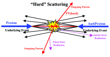
Figure 39: Illustration of the way the QCD Monte-Carlo models simulate a proton-antiproton collision in which a hard $2$-to-$2$ parton scattering with transverse momentum, $p_{T}({\rm hard})$, has occurred. The resulting event contains particles that originate from the two outgoing partons (plus initial and final-state radiation) and particles that come from the breakup of the proton and antiproton (“beam-beam remnants”). The “hard scattering” component consists of the outgoing two “jets” plus initial and final-state radiation. The “underlying event” is everything except the two outgoing hard scattered “jets” and consists of the “beam-beam remnants” plus possible contributions from the ”hard scattering” arising from initial and final-state radiation.

The “beam-beam remnants” are what is left over after a parton is knocked out of each of the initial two beam hadrons. It is the reason hadron-hadron collisions are more “messy” than electron-positron annihilations and no one really knows how it should be modeled. For the QCD Monte-Carlo models the “beam-beam remnants” are an important component of the “underlying event”. Also, it is possible that multiple parton scattering contributes to the “underlying event”. PYTHIA [313] models the “underlying event” in proton-antiproton collision by including multiple parton interactions. In addition to the hard $2$-to-$2$ parton-parton scattering and the “beam-beam remnants”, sometimes there is a second “semi-hard” $2$-to-$2$ parton-parton scattering that contributes particles to the “underlying event”.

Of course, from a certain point of view there is no such thing as an “underlying event” in a proton-antiproton collision. There is only an “event” and one cannot say where a given particle in the event originated. On the other hand, hard scattering collider “jet” events have a distinct topology. On the average, the outgoing hadrons “remember” the underlying the $2$-to-$2$ hard scattering subprocess. An average hard scattering event consists of a collection (or burst) of hadrons traveling roughly in the direction of the initial beam particles and two collections of hadrons (i.e., “jets”) with large transverse momentum. The two large transverse momentum “jets” are roughly back to back in azimuthal angle. One can use the topological structure of hadron-hadron collisions to study the “underlying event” [373, 374, 375]. The ultimate goal is to understand the physics of the “underlying event”, but since it is very complicated and involves both non-perturbative as well as perturbative QCD it seems unlikely that this will happen soon. In the mean time, we would like to tune the QCD Monte-Carlo models to do a better job fitting the “underlying event”. The “underlying event” is an unavoidable background to most collider observables. To find “new” physics at a collider it is crucial to have Monte-Carlo models that simulate accurately “ordinary” hard-scattering collider events. This report will compare collider observables that are sensitive to the “underlying event” with the QCD Monte-Carlo model predictions of PYTHIA 6.115 [313], /tt HERWIG 5.9 [339, 340, 236], and ISAJET 7.32 [376] and discuss the tuning of ISAJET and PYTHIA.

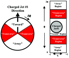
Figure 40: Illustrations of correlations in azimuthal angle $\Delta\phi$ relative to the direction of the leading charged jet in the event, chgjet#1. The angle $\Delta\phi=\phi-\phi_{\rm chgjet\#1}$ is the relative azimuthal angle between charged particles and the direction of chgjet#1. The“toward” region is defined by $|\Delta\phi|<60^{\circ}$ and $|\eta|\!<\!1$, while the “away” region is $|\Delta\phi|>120^{\circ}$ and $|\eta|\!<\!1$. The “transverse” region is defined by $60^{\circ}<|\Delta\phi|<120^{\circ}$ and $|\eta|\!<\!1$. Each region has an area in $\eta$-$\phi$ space of $4\pi/3$. On an event by event basis, we define “transMAX (“transMIN”) to be the maximum (minimum) of the two “transverse” pieces, $60^{\circ}<\Delta\phi<120^{\circ}$ and $|\eta|\!<\!1$, and $60^{\circ}<-\Delta\phi<120^{\circ}$ and $|\eta|\!<\!1$. “TransMAX” and “transMIN” each have an area in $\eta$-$\phi$ space of $2\pi/3$. The sum of “TransMAX” and “transMIN” is the total “transverse” region with area $4\pi/3$.

5.5.1 The “Transverse” Region

In a proton-antiproton collision large transverse momentum outgoing partons manifest themselves, in the laboratory, as a clusters of particles (both charged and neutral) traveling in roughly the same direction. These clusters are referred to as “jets”. In this analysis we examine only the charged particle component of “jets”. Our philosophy in comparing the QCD Monte-Carlo models with data is to select a region where the data is very “clean” so that “what you see is what you get” (almost). Hence, we consider only charged particles measured by the CDF central tracking chamber (CTC) in the region $p_{T}\!>\!0.5\,{\rm GeV/c}$ and $|\eta|\!<\!1$, where the track finding efficiency is high and uniform (estimated to be $92\%$ efficient) and we restrict ourselves to charged particle jets with transverse momentum less than $50{\rm\,GeV/c}$. The data presented here are uncorrected. Instead the theoretical Monte-Carlo models are corrected for the track finding efficiency by removing, on the average, $8\%$ of the charged particles. The theory curves have an error (statistical plus systematic) of about $5\%$. Thus, to within $10\%$ “what you see is what you get”.

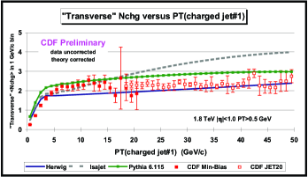
Figure 41: Data on the average number of charged particles ($p_{T}\!>\!0.5\,{\rm GeV/c}$, $|\eta|\!<\!1$) in the “transverse” region defined in Fig. 40 as a function of transverse momentum of the leading charged jet compared with the QCD Monte-Carlo predictions of HERWIG 5.9, ISAJET 7.32, and PYTHIA 6.115 with their default parameters and with $p_{T}\!({\rm hard})>3{\rm\,GeV/c}$. Each point corresponds to the $\langle\!N_{\rm chg}\!\rangle$  in a $1{\rm\,GeV/c}$ bin. The solid (open) points are the Min-Bias (JET20) data. The theory curves are corrected for the track finding efficiency and have an error (statistical plus systematic) of around $5\%$.

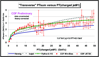
Figure 42: As for Fig 41 except that the average scalar $P_{T}$ is shown.

Charged particle “jets” are defined as clusters of charged particles ($p_{T}\!>\!0.5\,{\rm GeV/c}$, $|\eta|\!<\!1$) in “circular regions” of $\eta$-$\phi$ space with radius $R=0.7$. Every charged particle in the event is assigned to a “jet”, with the possibility that some jets might consist of just one charged particle. The transverse momentum of a charged jet, $P_{T}\!({\rm chgjet})$, is the scalar $p_{T}$ sum of the particles in the jet. We use the direction of the leading charged particle jet to define correlations in azimuthal angle, $\Delta\phi$. The angle $\Delta\phi=\phi-\phi_{\rm chgjet\#1}$ is the relative azimuthal angle between a charged particle and the direction of chgjet#1. The“toward” region is defined by $|\Delta\phi|<60^{\circ}$ and $|\eta|\!<\!1$, while the “away” region is $|\Delta\phi|>120^{\circ}$ and $|\eta|\!<\!1$. The “transverse” region is defined by $60^{\circ}<|\Delta\phi|<120^{\circ}$ and $|\eta|\!<\!1$. The three regions “toward”, “transverse”, and “away” are shown in Fig. 40. Each region has an area in $\eta$-$\phi$ space of $4\pi/3$. As illustrated in Fig. 40, the “toward” region contains the leading charged particle jet, while the “away” region, on the average, contains the “away-side” jet. The “transverse” region is perpendicular to the plane of the hard $2$-to-$2$ scattering and is therefore very sensitive to the “underlying event”.

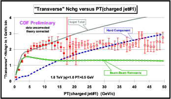
Figure 43: Data from Fig. 41 compared with the QCD Monte-Carlo predictions of ISAJET 7.32 (default parameters and $p_{T}\!({\rm hard})>3{\rm\,GeV/c}$). The predictions of ISAJET are divided into two categories: charged particles that arise from the break-up of the beam and target (beam-beam remnants), and charged particles that result from the outgoing jets plus initial and final-state radiation (hard scattering component). The theory curves are corrected for the track finding efficiency and have an error (statistical plus systematic) of around $5\%$.

Fig. 41 and Fig. 42 compare the “transverse” $\langle\!N_{\rm chg}\!\rangle$ and the “transverse” $\langle P_{T}{\rm sum}\!\rangle$, respectively, with the QCD Monte-Carlo predictions of HERWIG, ISAJET, and PYTHIA 6.115 with their default parameters and $p_{T}\!({\rm hard})>3{\rm\,GeV/c}$. The solid points are Min-Bias data and the open points are the JET20 data. The JET20 data connect smoothly to the Min-Bias data and allow us to study observables over the range $0.5<P_{T}\!({\rm chgjet}\#1)<50{\rm\,GeV/c}$. The average number of charged particles in the “transverse” region doubles in going from $P_{T}\!({\rm chgjet}\#1)$$=1.5{\rm\,GeV/c}$ to $2.5{\rm\,GeV/c}$ and then forms an approximately constant “plateau” for $P_{T}\!({\rm chgjet}\#1)$$>5{\rm\,GeV/c}$. If we suppose that the “underlying event” is uniform in azimuthal angle $\phi$ and pseudo-rapidity $\eta$, the observed $2.3$ charged particles at $P_{T}\!({\rm chgjet}\#1)$$=20{\rm\,GeV/c}$ translates to $3.8$ charged particles per unit pseudo-rapidity with $p_{T}\!>\!0.5\,{\rm GeV/c}$ (multiply by $3$ to get $360^{\circ}$, divide by $2$ for the two units of pseudo-rapidity, multiply by $1.09$ to correct for the track finding efficiency). We know that if we include all $p_{T}>50$ MeV/c there are, on the average, about four charged particles per unit rapidity in a “soft” proton-antiproton collision at 1.8 TeV [377]. The data in Fig. 41 imply that in the “underlying event” of a hard scattering there are, on the average, about $3.8$ charged particles per unit rapidity with $p_{T}\!>\!0.5\,{\rm GeV/c}$! Assuming a charged particle $p_{T}$ distribution of $e^{-2p_{T}}$ (see Fig. 52) implies that there are roughly $10$ charged particles per unit pseudo-rapidity with $p_{T}>0$ in the “underlying event” (factor of e). Since we examine only those charge particles with $p_{T}\!>\!0.5\,{\rm GeV/c}$, we cannot accurately extrapolate to low $p_{T}$, however, it is clear that the “underlying event” has a charge particle density that is at least a factor of two larger than the four charged particles per unit rapidity seen in “soft” proton-antiproton collisions at this energy.

The Min-Bias data were collected with a very “loose” trigger. The CDF Min-Bias trigger requirement removes elastic scattering and most of the single and double diffraction events, but keeps essentially all the “hard-scattering” events. In comparing with the QCD Monte-Carlo models we do require that the models satisfy the CDF Min-Bias trigger, however, for $P_{T}\!({\rm chgjet}\#1)$$>5{\rm\,GeV/c}$ essentially all the generated events satisfy the Min-Bias trigger (i.e., the Min-Bias trigger is unbiased for large $p_{T}$ “jets”). If we had enough Min-Bias events we would not need the JET20 data, but because of the fast fall-off of the cross section we run out of statistics at around $P_{T}\!({\rm chgjet}\#1)$$=20{\rm\,GeV/c}$ (that is why the Min-Bias data errors get large at around $20{\rm\,GeV/c}$). The JET20 data were collected by requiring at least $20{\rm\,GeV}$ of energy (charged plus neutral) in a cluster of calorimeter cells. We do not use the calorimeter information, but instead look only at the charged particles measured in the CTC in the same way we do for the Min-Bias data. The JET20 data is, of course, biased for low $p_{T}$ jets and we do not show the JET20 data below $P_{T}\!({\rm chgjet}\#1)$ around $20{\rm\,GeV/c}$. At large $P_{T}\!({\rm chgjet}\#1)$ values the JET20 data becomes unbiased and, in fact, we know this occurs at around $20{\rm\,GeV/c}$ because it is here that it agrees with the (unbiased) Min-Bias data.

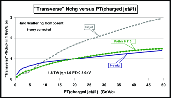
Figure 44: The “hard scattering” component (outgoing jets plus initial and final-state radiation) of the number of charged particles ($p_{T}\!>\!0.5\,{\rm GeV/c}$, $|\eta|\!<\!1$) in the “transverse” region defined in Fig. 40 as a function of the transverse momentum of the leading charged jet from the QCD Monte-Carlo predictions of HERWIG 5.9, ISAJET 7.32, and PYTHIA 6.115 with their default parameters and with $p_{T}\!({\rm hard})>3{\rm\,GeV/c}$. The curves are corrected for the track finding efficiency and have an error (statistical plus systematic) of around $5\%$.

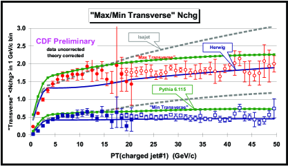
Figure 45: Data on the average number of “transMAX” and “transMIN” charged particles ($p_{T}\!>\!0.5\,{\rm GeV/c}$, $|\eta|\!<\!1$) as a function of the transverse momentum of the leading charged jet compared with the QCD Monte-Carlo predictions of HERWIG 5.9, ISAJET 7.32, and PYTHIA 6.115 with their default parameters and with $p_{T}\!({\rm hard})>3{\rm\,GeV/c}$. The solid (open) points are the Min-Bias (JET20) data. The theory curves are corrected for the track finding efficiency and have an error (statistical plus systematic) of around $5\%$.

We expect the “transverse” region to be composed predominately of particles that arise from the break-up of the beam and target and from initial and final-state radiation. This is clearly the case for the QCD Monte-Carlo models as can be seen in Figs. 7-9, where the predictions for the “transverse” region are divided into two categories: charged particles that arise from the break-up of the beam and target (beam-beam remnants), and charged particles that result from the outgoing jets plus initial and final-state radiation (hard scattering component). For PYTHIA the “beam-beam remnant” contribution includes contributions from multiple parton scattering. It is interesting to see that in the QCD Monte-Carlo models it is the “beam-beam remnants” that are producing the approximately constant “plateau”. The contributions from initial-state and final-state radiation increase as $P_{T}\!({\rm chgjet}\#1)$ increases. In fact, for ISAJET it is the sharp rise in the initial-state radiation component that is causing the disagreement with the data for $P_{T}\!({\rm chgjet}\#1)$$>20{\rm\,GeV/c}$. The hard scattering component of HERWIG and PYTHIA does not rise nearly as fast as the hard scattering component of ISAJET.

There are two reasons why the hard scattering component of ISAJET is different from HERWIG and PYTHIA. The first is due to different fragmentation schemes. ISAJET uses independent fragmentation, which produces too many soft hadrons when partons begin to overlap. The second difference arises from the way the QCD Monte-Carlos produce “parton showers”. ISAJET uses a leading-log picture in which the partons within the shower are ordered according to their invariant mass. Kinematics requires that the invariant mass of daughter partons be less than the invariant mass of the parent. HERWIG and PYTHIA modify the leading-log picture to include “color coherence effects” which leads to “angle ordering” within the parton shower. Angle ordering produces less high $p_{T}$ radiation within a parton shower which is what is seen in Fig. 44.

Of course, the origin of an outgoing particle (“beam-beam remnant” or “hard-scattering”) is not an experimental observable. Experimentally one cannot say where a given particle comes from. However, we do know the origins of particles generated by the QCD Monte-Carlo models and Figs. 7-9 show the composition of the “transverse” region as predicted by ISAJET, HERWIG, and PYTHIA.

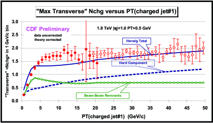
Figure 46: Data on the average number of “transMAX” charged particles ($p_{T}\!>\!0.5\,{\rm GeV/c}$, $|\eta|\!<\!1$) as a function of the transverse momentum of the leading charged jet compared with the QCD Monte-Carlo predictions of HERWIG 5.9 (default parameters and $p_{T}\!({\rm hard})>3{\rm\,GeV/c}$). The predictions of HERWIG are divided into two categories: charged particles that arise from the break-up of the beam and target (beam-beam remnants), and charged particles that result from the outgoing jets plus initial and final-state radiation (hard scattering component). The theory curves are corrected for the track finding efficiency and have an error (statistical plus systematic) of around $5\%$.

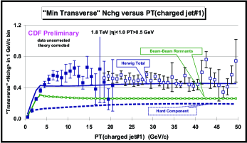
Figure 47: As for Fig 46 except that “transMIN” is shown.

5.5.2 Maximum and Minimum “Transverse” Regions

We now break up the “transverse” region into two pieces. As illustrated in Fig. 40, on an event by event basis, we define “transMAX” (“transMIN”) to be the maximum (minimum) of the two “transverse” pieces, $60^{\circ}<\Delta\phi<120^{\circ}$, $|\eta|\!<\!1$, and $60^{\circ}<-\Delta\phi<120^{\circ}$, $|\eta|\!<\!1$. Each has an area in $\eta$-$\phi$ space of $2\pi/3$ and what we previously referred to as the “transverse” region is the sum of “transMAX” and “transMIN”. One expects that “transMAX” will pick up more of the initial and final state radiation while “transMIN” should be more sensitive to the “beam-beam remnant” component of the “underlying event”. Furthermore, one expects that the “beam-beam remnant” component will nearly cancel in the difference, “transMAX” minus “transMIN”. If this is true then the difference, “transMAX” minus “transMIN”, would be more sensitive to the “hard scattering” component (i.e., initial and final-state radiation). I believe that this idea was first proposed by Bryan Webber and then implemented in a paper by Jon Pumplin [378] and then investigated in CDF by V. Tano [375]. . Fig. 45 show the data on the $\langle\!N_{\rm chg}\!\rangle$ for the“transMAX” and “transMIN” region as a function of the $P_{T}\!({\rm chgjet}\#1)$ compared with QCD Monte-Carlo predictions of HERWIG, ISAJET, and PYTHIA with their default parameters and $p_{T}\!({\rm hard})>3{\rm\,GeV/c}$. The data on $\langle P_{T}{\rm sum}\!\rangle$, show similar behaviour. Fig. 46 and Fig. 47, show the data on $\langle\!N_{\rm chg}\!\rangle$  for “transMAX”, and “transMIN”, compared with QCD Monte-Carlo predictions of HERWIG. The predictions of HERWIG are divided into two categories: charged particles that arise from the break-up of the beam and target (beam-beam remnants), and charged particles that result from the outgoing jets plus initial and final-state radiation (hard scattering component). It is clear from these plots that in the QCD Monte-Carlo models the “transMAX” is more sensitive to the “hard scattering component” of the “underlying event” while “transMIN” is more sensitive to the “beam-beam remnants”, especially at large values of $P_{T}\!({\rm chgjet}\#1)$. For example, for HERWIG at $P_{T}\!({\rm chgjet}\#1)$$=40{\rm\,GeV/c}$ the hard scattering component makes up $62\%$ of the “transMAX” $\langle\!N_{\rm chg}\!\rangle$ with $38\%$ coming from the “beam-beam remnants”. On the other hand, the hard scattering component makes up only $42\%$ of the “transMIN” $\langle\!N_{\rm chg}\!\rangle$ with $58\%$ coming from the “beam-beam remnants” at $P_{T}\!({\rm chgjet}\#1)$$=40{\rm\,GeV/c}$. Taking difference between “tansMAX” and “transMIN” does not completely remove the “beam-beam remnant” component, but reduces it to only about $32\%$ at $P_{T}\!({\rm chgjet}\#1)$$=40{\rm\,GeV/c}$.

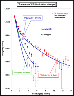
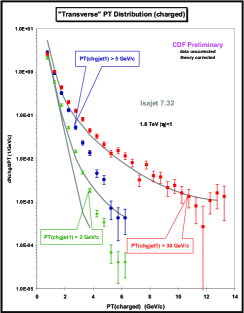
Figure 48: Data on the transverse momentum distribution of charged particles ($p_{T}\!>\!0.5\,{\rm GeV/c}$, $|\eta|\!<\!1$) in the “transverse” region for $P_{T}\!({\rm chgjet}\#1)$$>2{\rm\,GeV/c}$, $5{\rm\,GeV/c}$, and $30{\rm\,GeV/c}$, where chgjet#1 is the leading charged particle jet. Each point corresponds to $dN_{chg}/dp_{T}$ and the integral of the distribution gives the average number of charged particles in the transverse region, $\langle N_{chg}({\rm transverse})\rangle$. The data are compared with the QCD Monte-Carlo model predictions of HERWIG 5.9 (default parameters and $p_{T}\!({\rm hard})>3{\rm\,GeV/c}$). The theory curves are corrected for the track finding efficiency and have an error (statistical plus systematic) of around $5\%$. Right plot is compared with the QCD Monte-Carlo model predictions of ISAJET 7.32

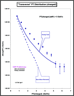
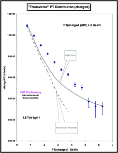
Figure 49: The data from Fig. 48 for $P_{T}\!({\rm chgjet}\#1)$$>5{\rm\,GeV/c}$ compared with the QCD Monte-Carlo model predictions of HERWIG 5.9 (left) and ISAJET (right) (default parameters and $p_{T}\!({\rm hard})>3{\rm\,GeV/c}$).

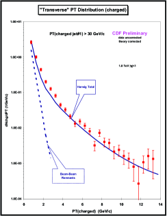
Figure 50: Data from Fig. 48 for $P_{T}\!({\rm chgjet}\#1)$$>30{\rm\,GeV/c}$ compared with the QCD Monte-Carlo model predictions of HERWIG 5.9 (default parameters and $p_{T}\!({\rm hard})>3{\rm\,GeV/c}$). The theory curves are corrected for the track finding efficiency and have an error (statistical plus systematic) of around $5\%$. The solid curve is the total (“hard scattering” plus “beam-beam remnants”) and the dashed curve shows the contribution arising from the break-up of the beam particles (“beam-beam remnants”).

5.5.3 The Transverse Momentum Distribution in the “Transverse” Region

Fig. 48 shows the data on the transverse momentum distribution of charged particles in the “transverse” region for $P_{T}\!({\rm chgjet}\#1)$$>2{\rm\,GeV/c}$, $5{\rm\,GeV/c}$, and $30{\rm\,GeV/c}$. Each point corresponds to $dN_{\rm chg}/dp_{T}$ and the integral of the distribution gives the average number of charged particles in the “transverse” region, $\langle\!N_{\rm chg}\!\rangle$, shown in Fig. 41. Fig. 41 shows only mean values, while Fig. 17 shows the distribution from which the mean is computed. In Fig. 48 the data are compared with the QCD hard scattering Monte-Carlo models predictions HERWIG and ISAJET Since these distributions fall off sharply as $p_{T}$ increases, it is essentially only the first few points at low $p_{T}$ that determine the mean. The approximately constant plateau seen in Fig. 41 is a result of the low $p_{T}$ points in Fig. 48 not changing much as $P_{T}\!({\rm chgjet}\#1)$ changes. However, the high $p_{T}$ points do increase considerably as $P_{T}\!({\rm chgjet}\#1)$ increases. This effect cannot be seen by simply examining the average number of “transverse” particles. Fig. 48 shows the growth of the “hard scattering component” at large $p_{T}$ in the ”transverse region” (i.e., three or more hard scattering jets).

For the QCD Monte-Carlo models the $p_{T}$ distribution in the “transverse” region, at low values of $P_{T}\!({\rm chgjet}\#1)$, is dominated by the “beam-beam remnant” contribution with very little “hard scattering” component. This can be seen in Fig. 49 which shows both the “beam-beam remnant” component together with the total overall predictions of HERWIG and ISAJET, respectively, for $P_{T}\!({\rm chgjet}\#1)$$>5{\rm\,GeV/c}$. For the QCD Monte-Carlo models the $p_{T}$ distribution in the “transverse” region, at low values of $P_{T}\!({\rm chgjet}\#1)$, measures directly the $p_{T}$ distribution of the “beam-beam remnants”. Both ISAJET and HERWIG have the wrong $p_{T}$ dependence in the “transverse” region due to a “beam-beam remnant” component that falls off too rapidly as $p_{T}$ increases. It is, of course, understandable that the Monte-Carlo models might be slightly off on the parameterization of the “beam-beam remnants”. This component cannot be calculated from perturbation theory and must be determined from data.

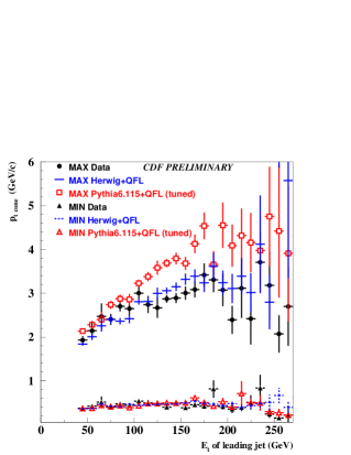
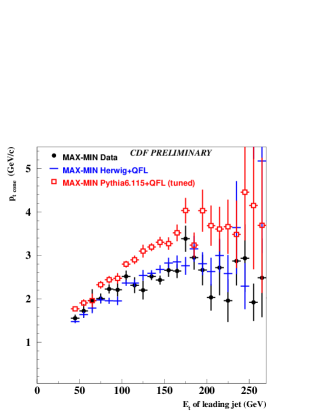
Figure 51: On the left is shown data on the average scalar $p_{T}$ sum of charged particles ($p_{T}>0.4{\rm\,GeV/c}$, $|\eta|\!<\!1$) within the maximum (MAX) and minimum (MIN) “transverse cones” versus the transverse energy of the leading (highest $E_{T}$) “calorimeter jet” compared with the QCD Monte-Carlo model predictions of HERWIG and PYTHIA.On the right is shown the difference (MAX-MIN) for each event.

Fig. 50 shows both the “beam-beam remnant” component together with the overall prediction of HERWIG for $P_{T}\!({\rm chgjet}\#1)$$>30{\rm\,GeV/c}$. Here the QCD Monte-Carlo models predict a large “hard scattering” component corresponding to the production of more than two large $p_{T}$ jets. HERWIG, ISAJET, and PYTHIA all do well at describing the high $p_{T}$ tail of this distribution. However, Fig. 48 shows that ISAJET produces too many charged particles at low $p_{T}$ which comes from an overabundance of soft particles produced in the hard scattering. Fig. 48 shows that the large rise in the transverse charged multiplicity from the hard scattering component of ISAJET seen in Fig. 43 comes from soft particles. This is to be expected from a model that employs independent fragmentation such as ISAJET. Independent fragmentation does not differ much from color string or cluster fragmentation for the hard particles, but independent fragmentation produces too many soft particles.

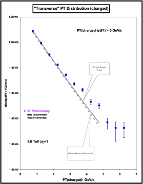
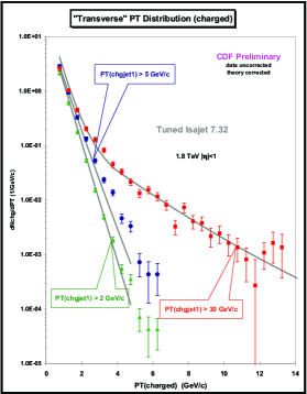
Figure 52: Data from Fig. 48 for $P_{T}\!({\rm chgjet}\#1)$$>5{\rm\,GeV/c}$ compared with the QCD Monte-Carlo model predictions of a “tuned” version of ISAJET 7.32 (CUTJET$=12{\rm\,GeV/c}$, $p_{T}\!({\rm hard})>3{\rm\,GeV/c}$). For the “tuned” version of ISAJET the $p_{T}$ distribution of the “beam-beam remnants” is generated according to $e^{-bp_{T}}$, where $b=2/({\rm\,GeV/c})$. The theory curves are corrected for the track finding efficiency and have an error (statistical plus systematic) of around $5\%$. The solid curve is the total (“hard scattering” plus “beam-beam remnants”) and the dashed curve shows the contribution arising from the break-up of the beam particles (“beam-beam remnants”).

Note that the transverse momentum distribution of the “beam-beam remnant” component for both HERWIG and ISAJET does not change in going from $P_{T}\!({\rm chgjet}\#1)$$>5{\rm\,GeV/c}$ to $P_{T}\!({\rm chgjet}\#1)$$>30{\rm\,GeV/c}$.

5.5.4 “Transverse Regions” Versus “Transverse Cones”

In a complementary CDF analysis, Valeria Tano [375] has studied the “underlying event” in hard scattering processes by defining “transverse cones” instead of “transverse regions”. The “transverse cones” (with radius in $\eta$-$\phi$ space of $R=0.7$) are located at the same pseudo-rapidity as the leading jet but with azimuthal angle $\Delta\phi=+90^{\circ}$ and $\Delta\phi=-90^{\circ}$ relative to the leading “jet”. In the cone analysis the “jet” is a “calorimeter jet” (charged plus neutrals) defined using the standard CDF cluster algorithm. Maximum (MAX) and minimum (MIN) “transverse” cones are determined, on an event-by-event basis, similar to the “transMAX” and “transMIN” regions described in Section III. Each “transverse cone” has an area in $\eta$-$\phi$ space of $\pi R^{2}=0.49\pi$ (compared with $0.67\pi$). Fig. 51 shows data at $1.8{\rm\,TeV}$ on the average scalar $p_{T}$ sum of charged particles ($p_{T}>0.4{\rm\,GeV/c}$, $|\eta|\!<\!1$) within the MAX and MIN “transverse cones” and the value of MAX-MIN for each event versus the transverse energy of the leading (highest $E_{T}$) “calorimeter jet”. (A similar analysis has been carried out at 630 GeV and a publication reporting the results from both energies is in preparation.) The data is compared with QCD hard scattering Monte-Carlo models predictions from HERWIG and PYTHIA. The “transverse cone” analysis covers the range $50<E_{T}({\rm calorimeter\ jet}\#1)<300{\rm\,GeV}$, while the “transverse region” analysis examines only charged particles and covers the range $0<$$P_{T}\!({\rm chgjet}\#1)$$<50{\rm\,GeV/c}$. One cannot directly compare the two analysis, but if one scales the low $E_{T}({\rm jet}\#1)$ points in Fig. 51 by the ratio of areas $0.67\pi/0.49\pi=1.36$, one gets approximate agreement with the high $P_{T}\!({\rm chgjet}\#1)$ points. Fig. 51 indicates that both HERWIG and PYTHIA correctly describe the MIN cone distributions but that PYTHIA generates too much energy for the MAX cone. Both analyses together provide a good handle on the “underlying event” in hard scattering processes.

5.5.5 Tuning the Models to Fit the “Underlying Event”

5.5.6 Tuning ISAJET

ISAJET generates the $p_{T}$ distribution of the “beam-beam remnants” according the power-law distribution $1/(1+P_{T}^{2}/b)^{4}$, where $b$ is chosen to give a mean $p_{T}$ of primary particles (i.e., before decay) of $450{\rm\,MeV/c}$. Fig. 49 indicates that this yields a $p_{T}$ distribution that falls off too rapidly. Since one does not know a priori how to parameterize the $p_{T}$ distribution of the “beam-beam remnants”, it is interesting to see if we can modify ISAJET to do a better job at fitting the data. Fig. 52 shows the $p_{T}$ distribution of the “beam-beam remnant” component together with the total overall predictions of a “tuned” version ISAJET. For the “tuned” version, ISAJET is modified to generate the $p_{T}$ distribution of the “beam-beam remnants” according to an exponential distribution of the form $e^{-bp_{T}}$, where $b=2/({\rm\,GeV/c})$. Also, for the tuned version of ISAJET the parameter CUTJET is increased from its default value of $6{\rm\,GeV/c}$ to $12{\rm\,GeV/c}$ in order to reduce the amount of initial-state radiation.

Fig. 53 compares the data on the average number of charged particles in the “transverse” region with the “tuned” version of ISAJET, where the predictions for the “transverse region are divided into two categories: charged particles that arise from the break-up of the beam and target (beam-beam remnants), and charged particles that result from the outgoing jets plus initial and final-state radiation (hard scattering component). If one compares Fig. 53 with Fig. 43 one sees that the tuned version of ISAJET has a larger “beam-beam remnant” plateau and less particles from the “hard-scattering” component (i.e., initial-state radiation). The “tuned” version of ISAJET does a much better job fitting the “underlying event” as can be seen by comparing Fig. 52 with Fig. 48. However, Fig. 53 shows that there are still too many charged particles in the “transverse” region at large $P_{T}\!({\rm chgjet}\#1)$ values.

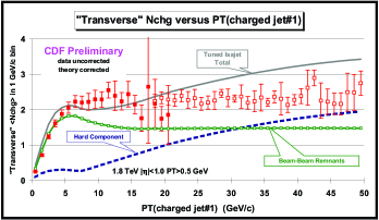
Figure 53: Data on the average number of charged particles ($p_{T}\!>\!0.5\,{\rm GeV/c}$, $|\eta|\!<\!1$) in the “transverse” region defined in Fig. 40 as a function of the transverse momentum of the leading charged jet compared with the QCD Monte-Carlo predictions of a “tuned” version of ISAJET 7.32 (CUTJET$=12{\rm\,GeV/c}$, $p_{T}\!({\rm hard})>3{\rm\,GeV/c}$). For the “tuned” version of ISAJET the $p_{T}$ distribution of the “beam-beam remnants” is generated according to $e^{-bp_{T}}$, where $b=2/({\rm\,GeV/c})$. The predictions are divided into two categories: charged particles that arise from the break-up of the beam and target (beam-beam remnants), and charged particles that result from the outgoing jets plus initial and final-state radiation (hard scattering component).

5.5.7 Tuning PYTHIA

Now that we have constructed collider observables that are sensitive to the “underlying event” we would like to tune the multiple parton interaction parameters of PYTHIA to fit the data. There are many tunable parameters. Here we consider only the parameters given in Table 1. The default values of the parameters are given in Table 2. Note that the PYTHIA default values sometimes change as the version changes

Table 14: PYTHIA multiple parton scattering parameters.

Parameter	Value	Description
MSTP(81)	$\mathrm{𝟎}$	Multiple-Parton Scattering off
	$1$	Multiple-Parton Scattering on
MSTP(82)	$1$	Multiple interactions assuming the same probability,
		with an abrupt cut-off $P_{T}{\rm min}$=PARP(81)
	$3$	Multiple interactions assuming a varying impact parameter
		and a hadronic matter overlap consistent with a
		single Gaussian matter distribution, with a smooth turn-off $P_{T0}$=PARP(82)
	$4$	Multiple interactions assuming a varying impact parameter
		and a hadronic matter overlap consistent with a
		double Gaussian matter distribution (governed by PARP(83) and PARP(84))
		with a smooth turn-off $P_{T0}$=PARP(82)

Table 15: Default values for some of the multiple parton scattering parameters of PYTHIA.

Parameter	PYTHIA 6.115	PYTHIA 6.125
MSTP(81)	$1$	$1$
MSTP(82)	$1$	$1$
PARP(81)	$1.4{\rm\,GeV/c}$	$1.9{\rm\,GeV/c}$
PARP(82)	$1.55{\rm\,GeV/c}$	$2.1{\rm\,GeV/c}$
PARP(83)	$0.5$	$0.5$
PARP(84)	$0.2$	$0.2$

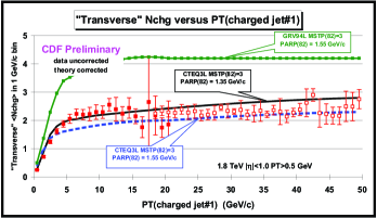
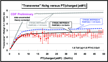
Figure 54: Data on the average number of charged particles ($p_{T}\!>\!0.5\,{\rm GeV/c}$, $|\eta|\!<\!1$) in the “transverse” region as a function of the transverse momentum of the leading charged jet compared with the QCD Monte-Carlo predictions of PYTHIA 6.115 with different structure functions and different multiple parton interaction parameters and with $p_{T}\!({\rm hard})>0{\rm\,GeV/c}$. The theory curves are corrected for the track finding efficiency and have an error (statistical plus systematic) of around $5\%$.

Fig. 54 shows data on the average number of charged particles in the “transverse” region compared with the QCD Monte-Carlo predictions of PYTHIA 6.115 with different structure functions and different multiple parton interaction parameters and with $p_{T}\!({\rm hard})>0{\rm\,GeV/c}$. For PYTHIA the amount of multiple parton scattering depends on the parton distribution functions (i.e., the structure functions) and hence the number of particles produced in the “transverse” region (i.e., the “underlying event”) changes if one changes the structure functions. HERWIG and ISAJET do not include multiple parton scattering and for them the number of particles in the “transverse” is essentially independent of the choice of structure functions.

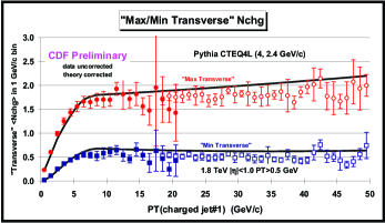
Figure 55: Data on the average number of “transMAX” and “transMIN” charged particles ($p_{T}\!>\!0.5\,{\rm GeV/c}$, $|\eta|\!<\!1$) as a function of the transverse momentum of the leading charged jet defined compared with the QCD Monte-Carlo predictions of PYTHIA 6.115 (tuned version, CTEQ4L, MSTP(82) = 4, PARP(82) = $1.4{\rm\,GeV/c}$, $p_{T}\!({\rm hard})>0{\rm\,GeV/c}$). The theory curves are corrected for the track finding efficiency and have an error (statistical plus systematic) of around $5\%$.

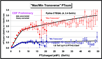
Figure 56: Data on the average scalar $p_{T}$ sum of “transMAX” and “transMIN” charged particles ($p_{T}\!>\!0.5\,{\rm GeV/c}$, $|\eta|\!<\!1$) as a function of the transverse momentum of the leading charged jet defined compared with the QCD Monte-Carlo predictions of PYTHIA 6.115 (tuned version, CTEQ4L, MSTP(82) = 4, PARP(82) = $1.4{\rm\,GeV/c}$, $p_{T}\!({\rm hard})>0{\rm\,GeV/c}$). The theory curves are corrected for the track finding efficiency and have an error (statistical plus systematic) of around $5\%$.

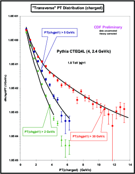
Figure 57: Data from Fig. 48 compared with the QCD Monte-Carlo model predictions of PYTHIA 6.115 (tuned version, CTEQ4L, MSTP(82) = 4, PARP(82) = $1.4{\rm\,GeV/c}$, $p_{T}\!({\rm hard})>0{\rm\,GeV/c}$). The theory curves are corrected for the track finding efficiency and have an error (statistical plus systematic) of around $5\%$.

Figs. 55-57 show the results of a “tuned” version of PYTHIA 6.115 with MSTP(82) = $4$ and PARP(82) = $2.4{\rm\,GeV/c}$ using the CTEQ4L structure functions. One must first choose a structure function and then tune the multiple parton scattering parameters for that structure function. In generating the PYTHIA curves in Figs. 30-35 we have taken $p_{T}\!({\rm hard})>0{\rm\,GeV/c}$. In general the perturbative $2$-to-$2$ parton scattering subprocesses diverge as $p_{T}({\rm hard})$ goes to zero. PYTHIA regulates these divergences using the same cut-off parameters that are used to regulate the multiple parton scattering cross section (see Table 1). This allows for the possibility of using PYTHIA to simultaneously describe both “soft” and “hard” collisions. Most of the CDF Min-Bias events are “soft”, with less than $3\%$ of the events having $P_{T}\!({\rm chgjet}\#1)$$>5{\rm\,GeV/c}$. There is no clear separation between “soft” and “hard” collisions, but roughly speaking $P_{T}\!({\rm chgjet}\#1)$$<2{\rm\,GeV/c}$ corresponds to “soft” Min-Bias collisions and demanding $P_{T}\!({\rm chgjet}\#1)$$>5{\rm\,GeV/c}$ assures a “hard” collision. Figs. 55-56 show that the “tuned” version of PYTHIA with $p_{T}\!({\rm hard})>0{\rm\,GeV/c}$ describes fairly well the transition between “soft” and “hard” collisions. The QCD Monte-Carlo models with $p_{T}\!({\rm hard})>3{\rm\,GeV/c}$ cannot describe the data for $P_{T}\!({\rm chgjet}\#1)$$<3{\rm\,GeV/c}$ (see Fig. 41 and Fig. 42), whereas PYTHIA with $p_{T}\!({\rm hard})>0{\rm\,GeV/c}$ seems to do a good job on the “transverse” observables as $P_{T}\!({\rm chgjet}\#1)$ goes to zero. Fig. 57 shows the data on the transverse momentum distribution of charged particles in the “transverse” region compared with the “tuned” version of PYTHIA 6.115 (CTEQ4L, MSTP(82) = $4$, PARP(82) = $2.4{\rm\,GeV/c}$). The fit is not perfect, but it is much better than the HERWIG prediction shown in Fig. 48. Multiple parton scattering produces more large $p_{T}$ particles in the “transverse” region, which is what is needed to fit the data. The $p_{T}$ distribution in the “transverse” region, at low values of $P_{T}\!({\rm chgjet}\#1)$, for the “tuned” version of PYTHIA is also dominated by the “beam-beam remnant” contribution as is the case for HERWIG (see Fig. 49). However, for PYTHIA the “beam-beam remnant” component includes contributions from multiple parton scattering, which results in a less steep $p_{T}$ distribution. Also, unlike ISAJET and HERWIG for PYTHIA the “beam-beam remnant” component increases as $P_{T}\!({\rm chgjet}\#1)$ increases due to multiple parton scattering.

5.5.8 Tuning HERWIG

The latest version of HERWIG includes a multiple-parton scattering option [379], which Jon Butterworth has tuned to fit some of the data presented here [380].

5.5.9 Summary

The “underlying event” in a hard scattering process is a complicated and interesting object which involves aspects of both non-perturbative and perturbative QCD. Studying the “transMAX” and “transMIN” pieces of the “transverse” region provides additional information not contained in the sum. In the QCD Monte-Carlo models the various components that make up the “underlying event” are weighted differently in “transMAX” and “transMIN” terms. The “transMAX” term preferentially selects the “hard component” of the “underlying event” (outgoing jets plus initial and final-state radiation) while the “transMIN” term preferentially selects the “beam-beam remnant” component. Unfortunately one cannot cleanly isolate a single component of the “underlying event” since all components contribute to both “transMAX”, “transMIN”, and to the difference. However, requiring the Monte-Carlo models to fit both “transMAX” and “transMIN” (or the sum and difference) puts additional constraints on the way the generators model the “underlying event”.

ISAJET (with independent fragmentation) produces too many (soft) particles in the “underlying event” with the wrong dependence on $P_{T}\!({\rm chgjet}\#1)$. HERWIG and PYTHIA modify the leading-log picture to include “color coherence effects” which leads to “angle ordering” within the parton shower and they do a better job describing the “underlying event”. Both ISAJET and HERWIG have the too steep of a $p_{T}$ dependence of the “beam-beam remnant” component of the “underlying event” and hence do not have enough “beam-beam remnants” with $p_{T}\!>\!0.5\,{\rm GeV/c}$. A modified version of ISAJET in which the “beam-beam remnants” are generated with an exponential distribution of the form $e^{-bp_{T}}$, where $b=2/({\rm\,GeV/c})$ improves the fit to the data. PYTHIA with multiple parton scattering does the best job at fitting the data.

The increased activity in the “underlying event” of a hard scattering over that observed in “soft” collisions cannot be explained solely by initial-state radiation. Multiple parton interactions provide a natural way of explaining the increased activity in the “underlying event” in a hard scattering. A hard scattering is more likely to occur when the “hard cores” of the beam hadrons overlap and this is also when the probability of a multiple parton interaction is greatest. For a soft grazing collision the probability of a multiple parton interaction is small. However, multiple parton interactions are very sensitive to the parton structure functions (PDF). You must first decide on a particular PDF and then tune the multiple parton interactions to fit the data.

One should not take the “tuned” version of PYTHIA 6.115 (CTEQ4L, MSTP(82) = $4$, PARP(82) = $2.4{\rm\,GeV/c}$) presented here too seriously. It is encouraging that it describes fairly well the ”transverse” region over the range $0<$$P_{T}\!({\rm chgjet}\#1)$$<50{\rm\,GeV/c}$ including the transition from “soft” to “hard” collisions. However, it is still not quite right. For example, it does not reproduce very well the multiplicity distribution of “soft” collisions. More work needs to be done in tuning the Monte-Carlo models. In addition, more work needs to be done before one can say for sure that the multiple parton interaction approach is correct. HERWIG without multiple parton scattering is not that far off the data. Maybe we simply need to change and improve the way the Monte-Carlo models handle the “beam-beam remnant” component.

References

- [1] D. Cavalli et al. hep-ph/0203056.
- [2] G. Azuelos et al. hep-ph/0204031.
- [3] W. Giele, S. Keller, and D. Kosower. hep-ph/0104052.
- [4] W. Giele and S. Keller. Phys. Rev., D58:094023, 1998.
- [5] J. Pumplin, D. Stump, and W. Tung. Phys. Rev., D65:014011, 2002.
- [6] J. Pumplin et al. Phys. Rev., D65:014013, 2002.
- [7] D. Stump et al. hep-ph/0101051. Phys. Rev., D65:014012, 2002.
- [8] G. D’Agostini. hep-ph/9512295.
- [9] S. Alekhin. hep-ex/0005042.
- [10] W. Eadie, D. Drijard, F. James, M. Roos, and B. Sadoulet. Statistical Methods in Experimental Physics, North Holland, 1971.
- [11] G. D’Agostini. Nucl. Instrum. Meth., A346:306–311, 1994.
- [12] M. Botje. hep-ph/0110123.
- [13] C. Pascaud and F. Zomer. preprint LAL-95-05.
- [14] M. Botje. Eur. Phys. J., C14:285–297, 2000.
- [15] M. Botje. Zeus Note 97–066.
- [16] J. Blümlein et al. hep-ph/9609400.
- [17] W. Furmanski and R. Petronzio. Z. Phys., C11:293, 1982.
- [18] O.V. Tarasov, A.A. Vladimirov, and A.Yu. Zharkov. Phys. Lett., B93:429, 1980.
- [19] S.A. Larin and J.A.M. Vermaseren. Phys. Lett., B303:334, 1993.
- [20] W. L. van Neerven and A. Vogt. Nucl. Phys., B568:263, 2000.
- [21] W. L. van Neerven and A. Vogt. Nucl. Phys., B588:345, 2000.
- [22] W. L. van Neerven and A. Vogt. Phys. Lett., B490:111, 2000.
- [23] S.A. Larin, T. van Ritbergen, and J.A.M. Vermaseren. Nucl. Phys., B427:41, 1994.
- [24] S.A. Larin, P. Nogueira, T. van Ritbergen, and J.A.M. Vermaseren. Nucl. Phys., B492:338, 1997.
- [25] A. Retey and J. A. M. Vermaseren. Nucl. Phys., B604:281, 2001.
- [26] S. Catani and F. F. Hautmann. Nucl. Phys., B427:475, 1994.
- [27] J. Blümlein and A. Vogt. Phys. Lett., B370:149, 1996.
- [28] V.S. Fadin and L.N. Lipatov. Phys. Lett., B429:127, 1998.
- [29] M. Ciafaloni and G. Camici. Phys. Lett., B430:349, 1998.
- [30] J.A. Gracey. Phys. Lett., B322:141, 1994.
- [31] J.F Bennett and J.A. Gracey. Nucl. Phys., B517:241, 1998.
- [32] Pietro Santorelli and Egidio Scrimieri. Phys. Lett., B459:599, 1999.
- [33] P. G. Ratcliffe. Phys. Rev., D63:116004, 2001.
- [34] C. Pascaud and F. Zomer. Preprint. hep-ph/0104013.
- [35] M. Dasgupta and G. P. Salam. hep-ph/0110213.
- [36] J. Blumlein and A. Vogt. Phys. Rev., D58:014020, 1998.
- [37] G. P. Salam and A. Vogt. in preparation.
- [38] H. L. Lai et al. Eur. Phys. J., C12:375, 2000.
- [39] M. Buza, Y. Matiounine, J. Smith, and W. L. van Neerven. Eur. Phys. J., C1:301, 1998.
- [40] S. A. Larin, T. van Ritbergen, and J. A. M. Vermaseren. Nucl. Phys., B438:278, 1995.
- [41] K. G. Chetyrkin, B. A. Kniehl, and M. Steinhauser. Phys. Rev. Lett., 79:2184, 1997.
- [42] Z. Bern, L. J. Dixon, and D. A. Kosower. Nucl. Phys., B412:751–816, 1994.
- [43] Z. Bern, L. J. Dixon, and D. A. Kosower. Phys. Lett., B302:299–308, 1993.
- [44] Z. Kunszt, A. Signer, and Z. Trocsanyi. Phys. Lett., B336:529–536, 1994.
- [45] A. Signer. Phys. Lett., B357:204–210, 1995.
- [46] Z. Bern, L. J. Dixon, D. A. Kosower, and S. Weinzierl. Nucl. Phys., B489:3–23, 1997.
- [47] Z. Bern, L. J. Dixon, and D. A. Kosower. Nucl. Phys., B513:3–86, 1998.
- [48] J. M. Campbell, E. W. N. Glover, and D. J. Miller. Phys. Lett., B409:503–508, 1997.
- [49] E. W. N. Glover and D. J. Miller. Phys. Lett., B396:257–263, 1997.
- [50] V. Del Duca, W. B. Kilgore, and F. Maltoni. Nucl. Phys., B566:252–274, 2000.
- [51] W. Beenakker et al. Phys. Rev. Lett., 87:201805, 2001.
- [52] L. Reina, S. Dawson, and D. Wackeroth. Phys. Rev., D65:053017, 2002.
- [53] V. Del Duca, W.B. Kilgore, C. Oleari, C. Schmidt, and D. Zeppenfeld. Nucl. Phys., B616:367–399, 2001.
- [54] T. Binoth, J. P. Guillet, and G. Heinrich. Nucl. Phys., B572:361–386, 2000.
- [55] Z. Bern and D. A. Kosower. Nucl. Phys., B379:451–561, 1992.
- [56] Z. Bern and D. A. Kosower. Nucl. Phys., B362:389–448, 1991.
- [57] Z. Bern, D. C. Dunbar, and T. Shimada. Phys. Lett., B312:277–284, 1993.
- [58] M. J. Strassler. Nucl. Phys., B385:145–184, 1992.
- [59] Z. Bern and D. C. Dunbar. Nucl. Phys., B379:562–601, 1992.
- [60] C. Schubert. Phys. Rept., 355:73–234, 2001.
- [61] A. Frizzo, L. Magnea, and R. Russo. Nucl. Phys., B604:92–120, 2001.
- [62] T. Binoth, J. P. Guillet, G. Heinrich, and C. Schubert. Nucl. Phys., B615:385–401, 2001.
- [63] S. Moch, J. A. M. Vermaseren, and M. Zhou. hep-ph/0108033.
- [64] R. Hamberg, W. L. van Neerven, and T. Matsuura. Nucl. Phys., B359:343–405, 1991.
- [65] R.V. Harlander and W.B. Kilgore. hep-ph/0201206.
- [66] E. B. Zijlstra and W. L. van Neerven. Nucl. Phys., B383:525–574, 1992.
- [67] A. D. Martin, R. G. Roberts, W. J. Stirling, and R. S. Thorne. hep-ph/0201127.
- [68] A. Gehrmann-De Ridder and E. W. N. Glover. Nucl. Phys., B517:269–323, 1998.
- [69] J. M. Campbell and E. W. N. Glover. Nucl. Phys., B527:264–288, 1998.
- [70] S. Catani and M. Grazzini. Phys. Lett., B446:143–152, 1999.
- [71] S. Catani and M. Grazzini. Nucl. Phys., B570:287–325, 2000.
- [72] V. Del Duca, A. Frizzo, and F. Maltoni. Nucl. Phys., B568:211–262, 2000.
- [73] F. A. Berends and W. T. Giele. Nucl. Phys., B313:595, 1989.
- [74] S. Catani. 1992. in Proceedings of the workshop on New technqiues for Calculating Higher Order QCD Corrections, report ETH-TH/93-01, Zurich (1992).
- [75] Z. Bern, L. J. Dixon, D. C. Dunbar, and D. A. Kosower. Nucl. Phys., B425:217–260, 1994.
- [76] Z. Bern, V. Del Duca, and C. R. Schmidt. Phys. Lett., B445:168–177, 1998.
- [77] D. A. Kosower. Nucl. Phys., B552:319–336, 1999.
- [78] Z. Bern, V. Del Duca, W. B. Kilgore, and C. R. Schmidt. Phys. Rev., D60:116001, 1999.
- [79] D. A. Kosower and P. Uwer. Nucl. Phys., B563:477–505, 1999.
- [80] S. Catani and M. Grazzini. Nucl. Phys., B591:435–454, 2000.
- [81] C. G. Bollini and J. J. Giambiagi. Nuovo Cim., B12:20–25, 1972.
- [82] J. F. Ashmore. Lett. Nuovo Cim., 4:289–290, 1972.
- [83] G. M. Cicuta and E. Montaldi. Nuovo Cim. Lett., 4:329–332, 1972.
- [84] G. ’t Hooft and M. J. G. Veltman. Nucl. Phys., B44:189–213, 1972.
- [85] F. V. Tkachov. Phys. Lett., B100:65–68, 1981.
- [86] K. G. Chetyrkin and F. V. Tkachov. Nucl. Phys., B192:159–204, 1981.
- [87] T. Gehrmann and E. Remiddi. Nucl. Phys., B580:485–518, 2000.
- [88] V. A. Smirnov and O. L. Veretin. Nucl. Phys., B566:469–485, 2000.
- [89] C. Anastasiou, E. W. N. Glover, and C. Oleari. Nucl. Phys., B575:416–436, 2000. Erratum: B585, 763, 2000.
- [90] C. Anastasiou, T. Gehrmann, C. Oleari, E. Remiddi, and J. B. Tausk. Nucl. Phys., B580:577–601, 2000.
- [91] S. Laporta. Int. J. Mod. Phys., A15:5087–5159, 2000.
- [92] P. A. Baikov and V. A. Smirnov. Phys. Lett., B477:367–372, 2000.
- [93] S. G. Gorishnii, S. A. Larin, L. R. Surguladze, and F. V. Tkachov. Comput. Phys. Commun., 55:381–408, 1989.
- [94] K. G. Chetyrkin, J. H. Kuhn, and A. Kwiatkowski. Phys. Rept., 277:189–281, 1996.
- [95] R.V. Harlander. Phys. Lett., B492:74–80, 2000.
- [96] S. Catani, D. de Florian, and M. Grazzini. JHEP, 05:025, 2001.
- [97] R.V. Harlander and W.B. Kilgore. Phys. Rev., D64:013015, 2001.
- [98] V. A. Smirnov. Phys. Lett., B460:397–404, 1999.
- [99] J. B. Tausk. Phys. Lett., B469:225–234, 1999.
- [100] C. Anastasiou, E. W. N. Glover, and C. Oleari. Nucl. Phys., B565:445–467, 2000.
- [101] A. T. Suzuki and A. G. M. Schmidt. J. Phys., A35:151–164, 2002.
- [102] C. Anastasiou, J. B. Tausk, and M. E. Tejeda-Yeomans. Nucl. Phys. Proc. Suppl., 89:262–267, 2000.
- [103] V. A. Smirnov. Phys. Lett., B491:130–136, 2000.
- [104] V. A. Smirnov. Phys. Lett., B500:330–337, 2001.
- [105] V. A. Smirnov. Phys. Lett., B524:129–136, 2002.
- [106] A. V. Kotikov. Phys. Lett., B267:123–127, 1991.
- [107] E. Remiddi. Nuovo Cim., A110:1435–1452, 1997.
- [108] M. Caffo, H. Czyz, S. Laporta, and E. Remiddi. Nuovo Cim., A111:365–389, 1998.
- [109] M. Caffo, H. Czyz, and E. Remiddi. Nucl. Phys., B581:274–294, 2000.
- [110] T. Gehrmann and E. Remiddi. Nucl. Phys. Proc. Suppl., 89:251–255, 2000.
- [111] T. Gehrmann and E. Remiddi. Nucl. Phys., B601:248–286, 2001.
- [112] T. Gehrmann and E. Remiddi. Nucl. Phys., B601:287–317, 2001.
- [113] T. Binoth and G. Heinrich. Nucl. Phys., B585:741–759, 2000.
- [114] N. Nielsen. Nova Acta Leopoldina (Halle)., 90:123, 1909.
- [115] L. Lewin. Polylogarithms and Associated Functions, North Holland (1981).
- [116] K. S. Kolbig. SIAM J. Math. Anal., 17:1232–1258, 1986.
- [117] K. S. Kolbig, J.A. Mignaco, and E. Remiddi. BIT, 10:38, 1970.
- [118] E. Remiddi and J. A. M. Vermaseren. Int. J. Mod. Phys., A15:725–754, 2000.
- [119] T. Gehrmann and E. Remiddi. Comput. Phys. Commun., 141:296–312, 2001.
- [120] T. Gehrmann and E. Remiddi. Comput. Phys. Commun., 144:200–223, 2002.
- [121] R. J. Gonsalves. Phys. Rev., D28:1542, 1983.
- [122] G. Kramer and B. Lampe. J. Math. Phys., 28:945, 1987.
- [123] Z. Bern, L. J. Dixon, and A. Ghinculov. Phys. Rev., D63:053007, 2001.
- [124] C. Anastasiou, E. W. N. Glover, C. Oleari, and M. E. Tejeda-Yeomans. Nucl. Phys., B601:318–340, 2001.
- [125] C. Anastasiou, E. W. N. Glover, C. Oleari, and M. E. Tejeda-Yeomans. Nucl. Phys., B601:341–360, 2001.
- [126] C. Anastasiou, E. W. N. Glover, C. Oleari, and M. E. Tejeda-Yeomans. Nucl. Phys., B605:486–516, 2001.
- [127] E. W. N. Glover, C. Oleari, and M. E. Tejeda-Yeomans. Nucl. Phys., B605:467–485, 2001.
- [128] Z. Bern, L. J. Dixon, and D. A. Kosower. JHEP, 01:027, 2000.
- [129] Z. Bern, A. De Freitas, and L.J. Dixon. hep-ph/0201161.
- [130] Z. Bern, A. De Freitas, and L. J. Dixon. JHEP, 09:037, 2001.
- [131] C. Anastasiou, E. W. N. Glover, and M. E. Tejeda-Yeomans. hep-ph/0201274.
- [132] Z. Bern, A. De Freitas, L. J. Dixon, A. Ghinculov, and H. L. Wong. JHEP, 11:031, 2001.
- [133] T. Binoth, E. W. N. Glover, P. Marquard, and J. J. van der Bij. hep-ph/0202266.
- [134] Z. Bern, A. De Freitas, L. Dixon, and H. L. Wong. hep-ph/0202271.
- [135] C. Anastasiou, E. W. N. Glover, C. Oleari, and M. E. Tejeda-Yeomans. Phys. Lett., B506:59–67, 2001.
- [136] E. W. N. Glover and M. E. Tejeda-Yeomans. JHEP, 05:010, 2001.
- [137] E. W. N. Glover, J. B. Tausk, and J. J. Van der Bij. Phys. Lett., B516:33–38, 2001.
- [138] A. B. Arbuzov, V.S. Fadin, E.A. Kuraev, L.N. Lipatov, N.P. Merenkov, and L. Trentadue. Nucl. Phys., B485:457–502, 1997.
- [139] L. W. Garland, T. Gehrmann, E. W. N. Glover, A. Koukoutsakis, and E. Remiddi. Nucl. Phys., B627:107–188, 2002.
- [140] S. Bethke. J. Phys., G26:R27, 2000.
- [141] J. A. Aguilar-Saavedra et al. hep-ph/0106315.
- [142] R. K. Ellis, D. A. Ross, and A. E. Terrano. Nucl. Phys., B178:421, 1981.
- [143] K. Fabricius, I. Schmitt, G. Kramer, and G. Schierholz. Zeit. Phys., C11:315, 1981.
- [144] W. T. Giele and E. W. N. Glover. Phys. Rev., D46:1980–2010, 1992.
- [145] S. Catani and M. H. Seymour. Nucl. Phys., B485:291–419, 1997. Erratum: B510, 503, 1997.
- [146] G. Kramer and B. Lampe. Z. Phys., C34:497, 1987. Erratum: C42, 504, 1989.
- [147] T. Matsuura and W. L. van Neerven. Z. Phys., C38:623, 1988.
- [148] T. Matsuura, S. C. van der Marck, and W. L. van Neerven. Nucl. Phys., B319:570, 1989.
- [149] S. Catani. Phys. Lett., B427:161–171, 1998.
- [150] A. Gehrmann-De Ridder, T. Gehrmann, and E. W. N. Glover. Phys. Lett., B414:354–361, 1997.
- [151] D. de Florian and M. Grazzini. Phys. Rev. Lett., 85:4678–4681, 2000.
- [152] D. de Florian and M. Grazzini. Nucl. Phys., B616:247–285, 2001.
- [153] E. A. Kuraev, L. N. Lipatov, and V. S. Fadin. Sov. Phys. JETP, 44:443–450, 1976.
- [154] V. Del Duca. Phys. Rev., D52:1527–1534, 1995.
- [155] E. A. Kuraev, L. N. Lipatov, and V. S. Fadin. Sov. Phys. JETP, 45:199–204, 1977.
- [156] I. I. Balitsky and L. N. Lipatov. Sov. J. Nucl. Phys., 28:822–829, 1978.
- [157] L. N. Lipatov. Sov. J. Nucl. Phys., 23:338–345, 1976.
- [158] V. S. Fadin and L. N. Lipatov. Nucl. Phys., B406:259–292, 1993.
- [159] L. N. Lipatov. Adv. Ser. Direct. High Energy Phys., 5, 1989.
- [160] V. Del Duca and E. W. N. Glover. JHEP, 10:035, 2001.
- [161] V. S. Fadin, M. I. Kotsky, and R. Fiore. Phys. Lett., B359:181–188, 1995.
- [162] V. S. Fadin, R. Fiore, and M. I. Kotsky. Phys. Lett., B387:593–602, 1996.
- [163] V. Fadin, R. Fiore, and A. Quartarolo. Phys. Rev., D53:2729–2741, 1996.
- [164] J. Blumlein, V. Ravindran, and W. L. van Neerven. Phys. Rev., D58:091502, 1998.
- [165] S. Mandelstam. Phys. Rev., 137:B949, 1965.
- [166] A. V. Bogdan, V. Del Duca, V. S. Fadin, and E. W. N. Glover. hep-ph/0201240.
- [167] V. S. Fadin and V. E. Sherman. Zh. Eksp. Teor. Fiz., 72:1640–1658, 1977.
- [168] M.L. Gell-Mann, M.and Goldberger, F.E. Low, E. Marx, and F. Zachariasen. Phys. Rev., 133:B145, 1964.
- [169] B. M. McCoy and T. T. Wu. Phys. Rev., D13:484–507, 1976.
- [170] V. S. Fadin and R. Fiore. Phys. Rev., D64:114012, 2001.
- [171] C. Balazs, J. Huston, and I. Puljak. Phys. Rev., D63:014021, 2001.
- [172] Y.L. Dokshitzer, D. Diakonov, and S. I. Troian. Phys. Rept., 58:269, 1980.
- [173] C. T. H. Davies and W.J. Stirling. Nucl. Phys., B244:337, 1984.
- [174] J.C. Collins, D.E. Soper, and G. Sterman. Nucl. Phys., B250:199, 1985.
- [175] S. Catani, D. de Florian, and M. Grazzini. Nucl. Phys., B596:299, 2001.
- [176] J. Kodaira and L. Trentadue. Phys. Lett., 112B:66, 1982.
- [177] S. Catani, E. D’Emilio, and L. Trentadue. Phys. Lett., B211:335, 1988.
- [178] A. Vogt. Phys. Lett., B497:228, 2001.
- [179] C. Balazs and C. P. Yuan. Phys. Rev., D56:5558, 1997.
- [180] A. Kulesza and W.J. Stirling. Eur. Phys. J., C20:349, 2001.
- [181] D. de Florian, M. Grazzini, and Z. Kunszt. Phys. Rev. Lett., 82:5209, 1999.
- [182] S. Dawson. Nucl. Phys., B359:283, 1991.
- [183] A. Djouadi, M. Spira, and P. M. Zerwas. Phys. Lett., B264:440, 1991.
- [184] M. Spira, A. Djouadi, D. Graudenz, and P. M. Zerwas. Nucl. Phys., B453:17, 1995.
- [185] S. Catani, D. de Florian, and M. Grazzini. JHEP, 01:015, 2002.
- [186] S. Catani, M.L. Mangano, P. Nason, and L. Trentadue. Nucl. Phys., B478:273, 1996.
- [187] M. Kramer, E. Laenen, and M. Spira. Nucl. Phys., B511:523, 1998.
- [188] A.D. Martin, R. G. Roberts, W.J. Stirling, and R. S. Thorne. Eur. Phys. J., C18:117, 2000.
- [189] E. Laenen, G. Sterman, and W. Vogelsang. Phys. Rev., D63:114018, 2001.
- [190] H. Contopanagos and G. Sterman. Nucl. Phys., B419:77, 1994.
- [191] B. R. Webber. Phys. Lett., B339:148, 1994.
- [192] G.P. Korchemsky and G. Sterman. Nucl. Phys., B437:415, 1995.
- [193] J.C. Collins and D.E. Soper. Nucl. Phys., B193:381, 1981.
- [194] A Kulesza, G. Sterman, and W. Vogelsang. hep-ph/0202251.
- [195] E. Laenen, G. Sterman, and W. Vogelsang. Phys. Rev. Lett., 84:4296, 2000.
- [196] T. Affolder (CDF Collab.). Phys. Rev. Lett., 84:845, 2000.
- [197] S. Tafat. JHEP, 05:004, 2001.
- [198] J.-W. Qiu and X.-F. Zhang. Phys. Rev. Lett., 86:2724, 2001.
- [199] J.C. Collins, D.E. Soper, and G. Sterman. Nucl. Phys., B308:833, 1988.
- [200] E.L. Berger et al. Summary of working group on QCD and strong interactions. To appear in the proceedings of APS / DPF / DPB Summer Study on the Future of Particle Physics (Snowmass 2001), Snowmass, Colorado, 30 Jun - 21 Jul 2001.
- [201] N. Kidonakis and G. Sterman. Nucl. Phys., B505:321, 1997.
- [202] N. Kidonakis and G. Sterman. Phys. Lett., B387:867, 1996.
- [203] E. Laenen and S. Moch. Phys. Rev., D59:034027, 1999.
- [204] N. Kidonakis. Int. J. Mod. Phys., A15:1245, 2000.
- [205] N. Kidonakis. Phys. Rev., D64:014009, 2001.
- [206] S. Kretzer, D. Mason, and F. Olness. hep-ph/0112191.
- [207] R. Meng, F.I. Olness, and D.E. Soper. Phys. Rev., D54:1919–1935, 1996.
- [208] P. M. Nadolsky, D. R. Stump, and C. P. Yuan. Phys. Rev., D64:114011, 2001.
- [209] P. Nadolsky, D. R. Stump, and C. P. Yuan. Phys. Rev., D61:014003, 2000.
- [210] M.A.G. Aivazis, J.C. Collins, F.I. Olness, and W.-K. Tung. Phys. Rev., D50:3102, 1994.
- [211] J.C. Collins. Phys. Rev., D58:094002, 1998.
- [212] B. Mele and P. Nason. Phys. Lett., B245:635, 1990.
- [213] B. Mele and P. Nason. Nucl. Phys., B361:626, 1991.
- [214] Yu.L. Dokshitzer, V.A. Khoze, and S.I. Troian. Phys. Rev., D53:89, 1996.
- [215] M. Cacciari and M. Greco. Nucl. Phys., B421:530, 1994.
- [216] M. Cacciari and M. Greco. Z. Phys., C69:459, 1996.
- [217] M. Cacciari et al. Nucl. Phys., B466:173, 1996.
- [218] M. Cacciari, M. Greco, and P. Nason. JHEP, 05:007, 1998.
- [219] M. Cacciari, S. Frixione, and P. Nason. JHEP, 03:006, 2001.
- [220] M. Cacciari and S. Catani. Nucl. Phys., B617:253, 2001.
- [221] P. Nason et al. hep-ph/0003142.
- [222] M. Cacciari, M. Greco, S. Rolli, and A. Tanzini. Phys. Rev., D55:2736, 1997.
- [223] M. Cacciari and M. Greco. Phys. Rev., D55:7134, 1997.
- [224] A. Heister et al. Phys. Lett., B512:30, 2001.
- [225] V.G. Kartvelishvili, A.K. Likhoded, and V.A. Petrov. Phys. Lett., B78:615, 1978.
- [226] R.L. Jaffe and L. Randall. Nucl. Phys., B412:79, 1994.
- [227] P. Nason and B.R. Webber. Phys. Lett., B395:355, 1997.
- [228] M. Beneke and V. M. Braun. Nucl. Phys., B454:253, 1995.
- [229] G. Sterman. Nucl. Phys., B281:310, 1987.
- [230] G. Sterman and W. Vogelsang. hep-ph/9910371. 1999.
- [231] E. Gardi. Nucl. Phys., B622:365, 2002.
- [232] L. Magnea. Nucl. Phys., B593:269, 2001.
- [233] L. Magnea. hep-ph/0109168.
- [234] S. Catani and L. Trentadue. Nucl. Phys., B327:323, 1989.
- [235] H. Contopanagos, E. Laenen, and G. Sterman. Nucl. Phys., B484:303, 1997.
- [236] S. Catani, B.R. Webber, and G. Marchesini. Nucl. Phys., B349:635, 1991.
- [237] J.-W. Qiu and G. Sterman. Nucl. Phys., B353:105, 1991.
- [238] R. Akhoury, M. G. Sotiropoulos, and V.I. Zakharov. Phys. Rev., D56:377, 1997.
- [239] M. Beneke and V. M. Braun. Phys. Lett., B348:513, 1995.
- [240] P. Ball, M. Beneke, and V. M. Braun. Nucl. Phys., B452:563, 1995.
- [241] Y.L. Dokshitzer, G. Marchesini, and B. R. Webber. Nucl. Phys., B469:93, 1996.
- [242] G. P. Korchemsky. in proceedings of 28th international conference on high-energy physics, warsaw, poland, july 1996. 1996.
- [243] E. Gardi and G. Grunberg. JHEP, 11:016, 1999.
- [244] E. Gardi and J. Rathsman. Nucl. Phys., B609:123, 2001.
- [245] E. Gardi and J. Rathsman. hep-ph/0201019.
- [246] E. Laenen, G. Oderda, and G. Sterman. Phys. Lett., B438:173, 1998.
- [247] N. Kidonakis, E. Laenen, S. Moch, and R. Vogt. Phys. Rev., D64:114001, 2001.
- [248] P. Nason, S. Dawson, and R.K. Ellis. Nucl. Phys., B303:607, 1988.
- [249] W. Beenakker, H. Kuijf, W.L. van Neerven, and J. Smith. Phys. Rev., D40:54, 1989.
- [250] W. Beenakker, W.L. van Neerven, R. Meng, G.A. Schuler, and J. Smith. Nucl. Phys., B351:507, 1991.
- [251] G. Oderda, N. Kidonakis, and G. Sterman. hep-ph/9906338.
- [252] G. Sterman and W. Vogelsang. hep-ph/0002132.
- [253] S. Forte. hep-ph/9910397.
- [254] V. Chekelian. hep-ex/0107053.
- [255] S. Chekanov et al. Eur. Phys. J., C21:443, 2001.
- [256] C. Adloff et al. Eur. Phys. J., C21:33, 2001.
- [257] R.D. Ball and S. Forte. Phys. Lett., B335:77, 1994.
- [258] A. De Rujula et al. Phys. Rev., D10:1649, 1974.
- [259] S. Forte and R.D. Ball. Acta Phys. Polon., B26:2097, 1995.
- [260] L. Mankiewicz, A. Saalfeld, and T. Weigl. Phys. Lett., B393:175, 1997.
- [261] V. S. Fadin, E. A. Kuraev, and L. N. Lipatov. Phys. Lett., B60:50, 1975.
- [262] R.D. Ball and S. Forte. Phys. Lett., B351:313, 1995.
- [263] R. K. Ellis, F. Hautmann, and B. R. Webber. Phys. Lett., B348:582, 1995.
- [264] G. Altarelli and G. Parisi. Nucl. Phys., B126:298, 1977.
- [265] V. N. Gribov and L. N. Lipatov. Yad. Fiz., 15:781, 1972.
- [266] L.D. McLerran. hep-ph/0104285.
- [267] R.D. Ball and S. Forte. Phys. Lett., B465:271, 1999.
- [268] G. Altarelli, R.D. Ball, and S. Forte. Nucl. Phys., B575:313, 2000.
- [269] M. Ciafaloni, D. Colferai, and G. P. Salam. Phys. Rev., D60:114036, 1999.
- [270] R.D. Ball and S. Forte. Phys. Lett., B405:317, 1997.
- [271] G. Altarelli, R.D. Ball, and S. Forte. Nucl. Phys., B599:383, 2001.
- [272] G. Altarelli, R.D. Ball, and S. Forte. Nucl. Phys., B621:359, 2002.
- [273] G. P. Salam. JHEP, 07:019, 1998.
- [274] R. D. Ball and R. K. Ellis. JHEP, 05:053, 2001.
- [275] G.C. Blazey et al. hep-ex/0005012.
- [276] S. Catani et al. hep-ph/0005114.
- [277] S.D. Ellis, J. Huston, and M. Tönnesmann. in preparation.
- [278] J.E. Huth et al. Toward a standardization of jet definitions. Presented at Summer Study on High Energy Physics, Reaearch Directions for the Decade, Snowmass, CO, Jun 25 - Jul 13, 1990.
- [279] S.D. Ellis and D.E. Soper. Phys. Rev., D48:3160–3166, 1993.
- [280] S. Catani, Yu.L. Dokshitzer, and B.R. Webber. Phys. Lett., B285:291–299, 1992.
- [281] S. Catani, Yu.L. Dokshitzer, M.H. Seymour, and B.R. Webber. Nucl. Phys., B406:187–224, 1993.
- [282] S.D. Ellis, Z. Kunszt, and D.E. Soper. Phys. Rev. Lett., 69:3615–3618, 1992.
- [283] S.D. Ellis. hep-ph/9306280.
- [284] B. Abbott, M. Bhattacharjee, D. Elvira, F. Nang, and H. Weerts. FERMILAB-PUB-97-242-E.
- [285] M.H. Seymour. Nucl. Phys., B513:269–300, 1998.
- [286] G. Marchesini et al. Comput. Phys. Commun., 67:465–508, 1992.
- [287] G. Corcella et al. JHEP, 01:010, 2001.
- [288] G. Corcella et al. hep-ph/9912396.
- [289] F. Abe et al. Phys. Rev., D45:1448–1458, 1992.
- [290] V.M. Abazov et al. hep-ex/0106032.
- [291] S.D. Ellis, Z. Kunszt, and D.E. Soper. Phys. Rev. Lett., 69:1496–1499, 1992.
- [292] S.D. Ellis, Z. Kunszt, and D.E. Soper. Phys. Rev. Lett., 64:2121, 1990.
- [293] S.D. Ellis, Z. Kunszt, and D.E. Soper. Phys. Rev., D40:2188, 1989.
- [294] S.D. Ellis, Z. Kunszt, and D.E. Soper. Phys. Rev. Lett., 62:726, 1989.
- [295] Torbjorn Sjostrand. Comput. Phys. Commun., 82:74–90, 1994.
- [296] T. Binoth, J. P. Guillet, E. Pilon, and M. Werlen. Eur. Phys. J., C16:311–330, 2000.
- [297] ATLAS collaboration. ATLAS Technical Proposal. CERN-LHCC-94-43.
- [298] ATLAS collaboration. ATLAS Detector and Physics Performance TDR. CERN-LHCC-99-14.
- [299] CMS collaboration. CMS Technical Proposal. CERN-LHCC-94-38.
- [300] CMS collaboration. CMS ECAL TDR. CERN-LHCC-97-33.
- [301] J. G. Branson et al. The ATLAS and CMS Collaboration. hep-ph/0110021.
- [302] S. Catani et al. Proc. CERN Workshop on Standard Model Physics (and more) at the LHC, Geneva 1999,ed. by G. Altarelli and M. Mangano. hep-ph/0005025.
- [303] T. Binoth. Talk given at 36th Rencontres de Moriond on QCD and Hadronic Interactions, Les Arcs, France, 17-24 March 2001. hep-ph/0105149.
- [304] M. Gluck, E. Reya, and A. Vogt. Z. Phys., C67:433–448, 1995.
- [305] T. Binoth, J. P. Guillet, E. Pilon, and M. Werlen. hep-ph/0203064.
- [306] B. A. Kniehl, G. Kramer, and B. Potter. Nucl. Phys., B582:514–536, 2000.
- [307] A. Pukhov et al. hep-ph/9908288.
- [308] T. Ishikawa et al. Grace manual: Automatic generation of tree amplitudes in standard models: Version 1.0. KEK-92-19.
- [309] G. Corcella et al. JHEP, 01:010, 2001.
- [310] T. Stelzer and W. F. Long. Comput. Phys. Commun., 81:357–371, 1994.
- [311] H. Baer, F. E. Paige, S. D. Protopopescu, and X. Tata. hep-ph/0001086.
- [312] F. A. Berends, H. Kuijf, B. Tausk, and W. T. Giele. Nucl. Phys., B357:32–64, 1991.
- [313] T. Sjostrand et al. Comput. Phys. Commun., 135:238–259, 2001.
- [314] F. Caravaglios, M. L. Mangano, M. Moretti, and R. Pittau. Nucl. Phys., B539:215–232, 1999.
- [315] M. L. Mangano, M. Moretti, and R. Pittau. hep-ph/0108069.
- [316] A. S. Belyaev et al. hep-ph/0101232.
- [317] T. Sjostrand, L. Lonnblad, and S. Mrenna. hep-ph/0108264.
- [318] K. Cranmer et al. http://pheno.physics.wisc.edu/Software/MadCUP/.
- [319] M.L. Mangano et al. http://cern.ch/mlm/alpgen/alpgen.html.
- [320] V. Ilyin. 2002. Presented at the Physics and Detectors for a 90 to 800 GeV Linear Collider Second Workshop of the Extended ECFA/DESY Study in St. Malo, France.
- [321] B. P. Kersevan and E. Richter-Was. hep-ph/0201302.
- [322] M. Dobbs. hep-ph/0111234.
- [323] T. Sjostrand et al. in Z Physics at LEP 1, vol. 3, edited by G. Altarelli, R. Kleiss and C. Verzegnassi, CERN 89-08 (Geneva, 1989), p. 327.
- [324] M. Dobbs and J. B. Hansen. Comput. Phys. Commun., 134:41–46, 2001.
- [325] L. Garren, I. G. Knowles, T. Sjostrand, and T. Trippe. Eur. Phys. J., C15:205–207, 2000.
- [326] H. Plothow-Besch. Comput. Phys. Commun., 75:396–416, 1993. refer to http://consult.cern.ch/writeup/pdflib/.
- [327] B. Kersevan and E. Richter-Was. 2001. ATLAS Physics Communication, ATL-COM-PHYS-2001-013.
- [328] B. Kersevan and E. Richter-Was. 2001. ATLAS Physics Communication, ATL-COM-PHYS-2001-014.
- [329] B. Kersevan and E. Richter-Was. 2001. ATLAS Physics Communication, ATL-COM-PHYS-2001-025.
- [330] ATLAS Collaboration. ATLAS Detector and Physics Performance TDR. 1999. CERN-LHCC/99-15.
- [331] G. Jarlskog and D. (editors) Rein. Proceedings of the large hadron collider workshop, aachen. 1990. CERN 90-10/ECFA 90-133.
- [332] B. van Eijk and R. Kleiss. Proceedings of the large hadron collider workshop, aachen. page 184, 1990. CERN 90-10/ECFA 90-133.
- [333] B. van Eijk et al. Nuc. Phys. B, 292:1, 1987.
- [334] M. Della Negra et al. Proceedings of the large hadron collider workshop, aachen. page 509, 1990. CERN 90-10/ECFA 90-133.
- [335] J. M. Campbell and R. K. Ellis. Phys. Rev., D62:114012, 2000.
- [336] J. Gunion. Phys. Rev. Lett., 72:199, 1994.
- [337] E. Richter-Was and M. Sapinski. 1998. ATLAS Internal Note, ATL-PHYS-98-132.
- [338] M. L. Mangano, P. Nason, and G. Ridolfi. Nucl. Phys., B405:507–535, 1993.
- [339] G. Marchesini and B. R. Webber. Nucl. Phys., B310:461, 1988.
- [340] I. G. Knowles. Nucl. Phys., B310:571, 1988.
- [341] M. L. Mangano, M. Moretti, and R. Pittau. http://mlm.home.cern.ch/mlm/wbb/wbb.html.
- [342] F. Mazzucato. Studies on the standard model self-couplings. ATLAS Internal Note, in preparation.
- [343] J. Hilgart, R. Kleiss, and F. Le Diberder. 75:191–218, 1993.
- [344] F. A. Berends, R. Pittau, and R. Kleiss. Comput. Phys. Commun., 85:437–452, 1995.
- [345] F. A. Berends, C. G. Papadopoulos, and R. Pittau. Comput. Phys. Commun., 136:148–172, 2001.
- [346] R. Kleiss and R. Pittau. Comput. Phys. Commun., 83:141–146, 1994.
- [347] G. P. Lepage. J. Comput. Phys., 27:192, 1978.
- [348] T. Ohl. hep-ph/9911437.
- [349] S. Jadach, B. F. L. Ward, and Z. Was. Comput. Phys. Commun., 130:260–325, 2000.
- [350] H. U. Bengtsson and G. Ingelman. Comput. Phys. Commun., 34:251, 1985.
- [351] G. Miu and T. Sjostrand. Phys. Lett., B449:313–320, 1999.
- [352] G. Corcella and M. H. Seymour. Nucl. Phys., B565:227–244, 2000.
- [353] Y. Chen, John C. Collins, and N. Tkachuk. JHEP, 06:015, 2001.
- [354] J. C. Collins and F. Hautmann. JHEP, 03:016, 2001.
- [355] A. Djouadi et al. hep-ph/0002258.
- [356] C. Balazs and C. P. Yuan. Phys. Lett., B478:192–198, 2000.
- [357] G. T. Bodwin, S. J. Brodsky, and G. P. Lepage. Factorization of the drell-yan cross-section. Presented at 20th Rencontre de Moriond, Les Arcs, France, Mar 10-17, 1985.
- [358] M. Bengtsson, T. Sjostrand, and M. van Zijl. Z. Phys., C32:67, 1986.
- [359] V. N. Gribov and L. N. Lipatov. Yad. Fiz., 15:1218–1237, 1972.
- [360] Yu. L. Dokshitzer. Sov. Phys. JETP, 46:641–653, 1977.
- [361] R. Odorico. Nucl. Phys., B172:157, 1980.
- [362] R.K. Ellis, W.J. Stirling, and B.R. Webber. Qcd and collider physics; monogr. part. phys. nucl. phys. cosmol. (1996).
- [363] T. Sjostrand. Phys. Lett., B157:321, 1985.
- [364] G. Marchesini and B. R. Webber. Nucl. Phys., B238:1, 1984.
- [365] Y. L. Dokshitzer, D. Diakonov, and S. I. Troian. Phys. Lett., B79:269–272, 1978.
- [366] G. Parisi and R. Petronzio. Nucl. Phys., B154:427, 1979.
- [367] S. D. Ellis, N. Fleishon, and W. J. Stirling. Phys. Rev., D24:1386, 1981.
- [368] J. C. Collins and D. E. Soper. Phys. Rev. Lett., 48:655, 1982.
- [369] G. Altarelli, R. K. Ellis, M. Greco, and G. Martinelli. Nucl. Phys., B246:12, 1984.
- [370] G. Altarelli, R. K. Ellis, and G. Martinelli. Z. Phys., C27:617, 1985.
- [371] P. B. Arnold and R. P. Kauffman. Nucl. Phys., B349:381–413, 1991.
- [372] R. K. Ellis and S. Veseli. Nucl. Phys., B511:649–669, 1998.
- [373] T. Affolder et al. FERMILAB-PUB-01/211-E (to appear in Phys. Rev. D).
- [374] R. Field (for the CDF Collaboration). The underlying event in large transverse momentum charged jets. presented at DPF2000, Columbus, OH, August 11, 2000.
- [375] V. Tano (for the CDF Collaboration. The underlying event in jet and minimum bias events. presented at ISMD2001, Datong, China, Sept. 2001.
- [376] F. E. Paige and S. D. Protopopescu. Isajet 5.20: A monte carlo event generator for p p and anti-p p interactions. Invited talk given at Workshop on Observable Standard Model Physics at the SSC: Monte Carlo Simulation ad Detector Capabilities, Los Angeles, CA, Jan 15-24, 1986.
- [377] F. Abe et al. Phys. Rev., D41:2330, 1990.
- [378] J. Pumplin. Phys. Rev., D57:5787–5792, 1998.
- [379] J. M. Butterworth, J. R. Forshaw, and M. H. Seymour. Z. Phys., C72:637–646, 1996.
- [380] J. M. Butterworth. Talk presented by Jon Butterworth at Snowmass 2001.