Before and After: How has the SNO neutral current measurement changed things?

Abstract:

We present “Before and After” global oscillation solutions, as well as predicted “Before and After” values and ranges for ten future solar neutrino observables (for BOREXINO, KamLAND, SNO, and a generic $p-p$ neutrino detector). The “Before” case includes all solar neutrino data (and some theoretical improvements) available prior to April 20, 2002 and the “After” case includes, in addition, the new SNO data on the CC, NC, and day-night asymmetry. We have performed global analyses using the full SNO day-night energy spectrum and, alternatively, using just the SNO NC and CC rates and the day-night asymmetry. The LMA solution is the only currently allowed MSW oscillation solution at $\sim 99$% CL. The LOW solution is allowed only at more than $2.5\sigma$, SMA is now excluded at $3.7\sigma$ or $4.7\sigma$ depending upon analysis strategy, and pure sterile oscillations are excluded at more than $4.7\sigma$. Small mixing angles are “out” (pure sterile is “way out”); MSW with large mixing angles is definitely “in.” Vacuum oscillations are allowed at $3\sigma$, but not at $2\sigma$. Precise maximal mixing is excluded at $3.2\sigma$ for MSW solutions and at more than $2.8\sigma$ for vacuum solutions. Most of the predicted values for future observables for the BOREXINO, KamLAND, and future SNO measurements are changed only by minor amounts by the inclusion of the recent SNO data. In order to test the robustness of the allowed neutrino oscillation regions that are inferred from the measurements and the predicted values for future solar neutrino observables, we have carried out calculations using a variety of strategies for analyzing the SNO and other experimental data.

1 Introduction

The goal of this paper is to assess the impact of recent SNO measurements  [1, 2, 3] on the allowed regions of neutrino oscillation parameters and on the predicted values of the most important future solar neutrino observables. The SNO collaboration has reported a neutral current (NC) measurement of the active ⁸B solar neutrino flux and related measurements of the day-night asymmetry, as well as improved determinations of the charged current (CC) and neutrino-electron scattering rate.

We are concerned that global solutions for oscillation parameters depend upon the assumption that the errors are well understood for all of the reported measurements in the chlorine, gallium, Super-Kamiokande, and SNO experiments. There are many cases in the past for which similar assumptions have proved misleading. Therefore, we focus our study on determining the robustness of our conclusions regarding the currently allowed oscillation parameters and the predicted values of new solar neutrino observables. We test the robustness of the conclusions about allowed oscillation parameters by using three different analysis strategies. We also compute predicted values for future solar neutrino observables with the oscillation parameters that are currently allowed as well with the oscillation parameters that were allowed before the recent SNO measurements. In addition, we treat the SNO data in two different ways: a) with the aid of a two-step process (discussed in section 2.5) and b) using the full SNO day-night energy spectrum (see section 5.4) used by the SNO collaboration. In our view, a necessary condition for a result to be regarded as ”robust” is that the result not change significantly as we vary the analysis procedures among the different plausible possibilities listed above.

Perhaps the most remarkable and encouraging result of our analysis is that the allowed regions for the oscillation parameters, $\Delta m^{2}$ and $\tan^{2}\theta$, the predicted values of ten future solar neutrino observables, and the inferred total ⁸B neutrino flux are all rather robust with respect to the choices among the different analysis procedures. The inferences from the available data are relatively independent of the details of the analysis procedures. This conclusion will be justified quantitatively in section 5 and summarized in section 6.

We begin in section 2 by deriving, using the two-step procedure for the SNO data, the currently allowed regions in neutrino oscillation space that are obtained with three different analysis strategies (see figure 1), each strategy previously advocated by a different set of authors. The global solutions obtained here are calculated using the methods described in our recent paper [4] (see especially section 3.3 of ref. [4]) but also include some refinements in addition to the new SNO data. For example, we take account of the energy dependence and correlations of the errors in the neutrino absorption cross sections for the chlorine and gallium solar neutrino experiments as described in the Appendix of ref. [5]. We also include the recently reported SAGE [6] data for 11 years of observation and the zenith angle-recoil energy spectrum data presented by the Super-Kamiokande collaboration after $1496$ days of observations [7] . Where required, we use the predicted fluxes and their errors from the BP00 standard solar model [8].

We present in section 3, and especially in figure 3,  a “Before and After” comparison of the globally allowed neutrino oscillation solutions (see figure 3). In the “Before” case, we use all the solar neutrino data (see refs. [9, 10, 11, 12, 13, 14, 15]) that were published or had appeared publicly before April 20, 2002, the date that the SNO NC and day-night asymmetry were first published. In the “After” case, we include in addition measurements reported in the two recent papers [1, 2] by the Sudbury Neutrino Observatory (SNO) collaboration.

What are the predicted values of the ten most informative quantities that can be measured in the reasonably near future in solar neutrino experiments? We use in section 4 the allowed regions in neutrino parameter space (obtained in section 2) to predict in table 2 the expected range of the most promising quantities that can be measured accurately in the BOREXINO  [16] and KamLAND [17] ${\rm{}^{7}Be}$ solar neutrino experiments and in the KamLAND reactor experiment, as well as the spectrum distortion and the day-night asymmetry in the SNO CC measurements. We also include predictions for a generic $p-p$ neutrino-electron scattering detector. To assess the robustness of the predictions, we compare the values predicted using the “After April 20, 2002” global solution (table 2) with the values predicted using the “Before April 20, 2002” solution (table 3).

We summarize and discuss our conclusions in section 6.

We do not discuss in this paper the implications of the agreement between the measured [1] flux of active ⁸B solar neutrinos and the predicted [8] standard solar model ⁸B neutrino flux. The agreement is accidentally too good to be true [see eq. (6)]. As more measurements are made of the neutrino flux and of the solar model parameters the agreement should become less precise. We are aware of several recent and ongoing measurements, which are currently not in good agreement, for the low energy cross section factor $S_{17}$, to which the calculated standard solar model ⁸B neutrino flux is proportional. Until the new laboratory measurements of $S_{17}$ converge to a better defined range, we continue to use the standard value adopted in BP00.

2 Global oscillation solutions

We describe in section 2.1 the oscillation solutions that are allowed with three different analysis prescriptions (see figure 1). We have at different times used all three of the analysis strategies and various colleagues have advocated strongly one or the other of the strategies described here. Given the recent SNO NC measurement, we now prefer the strategy in which the ⁸B neutrino flux is treated as a free parameter. This strategy is implemented in figure 1a (see the discussion below). A comparison of the results obtained using the three strategies allows one to test the robustness of any conclusion to the method of analysis.

We present in section 2.2 and table 1 the best-fit oscillation parameters for the allowed and the disfavored solutions, treating the ⁸B neutrino flux as a free parameter. We discuss in this section the CL at which different oscillation solutions are acceptable.

In section 2.3, we present and discuss the allowed ranges for $\Delta m^{2}$, $\tan^{2}\theta$, and the total active flux of ⁸B solar neutrinos.

We describe in section 2.4 and in figure 2 the predicted dependence of the survival probability as a function of energy and of day or night for the best-fit LMA, LOW, and vacuum solutions. Figure 2 in particular provides a succinct overview of the energy and day-night dependences of the best-fit survival probabilities.

The SNO experiment detects CC, NC, ES ($\nu-e$ scattering), and background events. The rates from these different processes are correlated because they are, with the present data, observed most accurately in a mode in which all of the events are considered together and a simultaneous solution is made for each of the separate processes using their known angular dependences (with respect to the solar direction) and their radial dependences in the detector, as well as information from direct measurements of the background  [1, 2, 3]. Details of how this analysis is done are given in refs. [2, 3].

Since the different processes are coupled together in the analysis, the inferred values for the measured fluxes in each of the CC, NC, and ES modes depend upon the assumed distortion of the CC and ES recoil energy spectra, which in turn depend upon the assumed $\Delta m^{2}$ and $\tan^{2}\theta$. In order to avoid this cycle, the SNO collaboration presented [2] results for the CC, NC, and ES fluxes that were determined by assuming that the CC and ES recoil energy spectra are undistorted by neutrino oscillations or any other new physics.

The fluxes inferred using the hypothesis of undistorted energy spectra has been used by ref. [20] in their analyses of the SNO data. This approximation is excellent for the LMA and LOW solutions, as we shall show later in this section (see, e.g., results quoted in section 2.2), because for these solutions the expected distortions are indeed small. The approximation is less accurate for other solutions in which the distortions are more significant.

In order to obtain the results presented in the following subsections, we used a two-step procedure to take account, for each value of $\Delta m^{2}$ and $\tan^{2}\theta$, of the energy dependence of the survival probability. We have used in these calculations experimental data provided by the SNO collaboration [3]. We describe how we have carried out the details of this analysis in section 2.5. The results obtained using the full SNO day-night energy spectrum are presented in section 5.

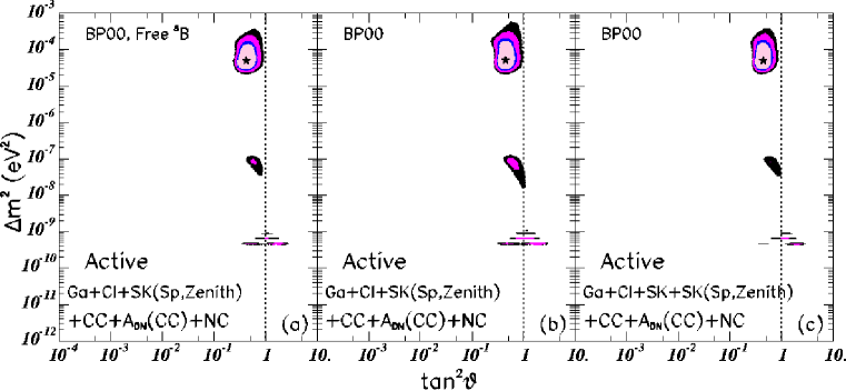
Figure 1: Global neutrino oscillation solutions for three different analysis strategies. The strategy used in constructing panel (a) treats the ⁸B solar neutrino flux as a free parameter to be determined by the experimental data together with $\Delta m^{2}$ and $\tan^{2}\theta$. The strategies corresponding to panels (b) and (c) include the theoretical uncertainty in the ⁸B neutrino flux, but differ in how they treat the total rate measured in the Super-Kamiokande experiment. The input data used in constructing figure 1 include the neutrino fluxes and uncertainties predicted by the BP00 solar model [8] and the total measured CC and NC event rates from the SNO experiment  [1], the SNO day-night asymmetry [2], the Chlorine [10] and Gallium (averaged) [6, 11, 12, 13] event rates, as well as the zenith angle-recoil energy spectrum data presented by Super-Kamiokande [14]. The rates from the GALLEX/GNO and SAGE experiments have been averaged to provide a unique data point ($72.4\pm 4.7$ SNU). The CL contours shown in the figure are $90$%, $95$%, $99$%, and $99.73$% ($3\sigma$). The global best-fit points are marked by a star.

2.1 Three strategies

Figure 1 shows the allowed ranges of the neutrino oscillation parameters, $\Delta m^{2}$ and $\tan^{2}\theta$, that were computed using the three different analysis approaches that have been used previously in the literature. We use the analysis methods and procedures described in refs. [4, 5, 27, 28, 29, 21, 30]), see especially section 3.3 of ref. [4] and the Appendix of ref. [5]. We follow refs. [31, 32] in using $\tan^{2}\theta$ (rather than $\sin^{2}2\theta$) in order to display conveniently the solutions on both sides of $\theta=\pi/4$.

Figure 1a presents the result for our standard analysis, (a), the free ${\rm{}^{8}B}$ analysis. The strategy used in this standard analysis takes account of the BP00 predicted fluxes and uncertainties for all neutrino sources except for ⁸B neutrinos. The normalization of the ⁸B neutrino flux is treated as a free parameter for analysis strategy (a) but is constrained by the BP00 prediction and error for strategies (b) and (c). Analysis strategy (a) considers all the experimental data except for the Super-Kamiokande total event rate. The recoil electron zenith angle-recoil energy spectrum data represent the Super-Kamiokande total rate in this approach. Details of the treatment of the Super-Kamiokande errors are given in Sec. 5.4.

Figure 1b displays the results of a calculation, analysis strategy (b), which is the same as for the standard case, figure 1a, except that the ${\rm{}^{8}B}$ neutrino flux is constrained by the BP00 solar model prediction. Prior to the SNO measurement of the NC flux [1], (b) was our standard analysis strategy (cf. ref. [4]). Following the SNO NC measurement, we prefer to use the neutrino data to determine the flux normalization and therefore to test, rather than assume, the standard solar model prediction for the ⁸B neutrino flux.

Figure 1c was constructed by an analysis similar to that used to construct figure 1b except that for figure 1b the total Super-Kamiokande rate is included explicitly together with a free normalization factor for the zenith angle-recoil energy spectrum of the recoil electrons. This procedure has been used especially effectively by the Bari group [23]

In all cases, we have accounted for the energy and time dependence of the Super-Kamiokande data by using their zenith angle-recoil energy spectrum data. The available Super-Kamiokande zenith angle-recoil energy spectrum consists of 44 data points, corresponding to six night bins and one day bin for six energy bins between 5.5 and 16 MeV electron recoil energy, plus two daily averaged points for the lowest ($5.0<E<5.5$ MeV) and the highest ($E>16$ MeV) energy bins. Alternatively, one could use their day-night energy spectra as given in 19 energy bins each for the day and for the night periods. Using the more complete zenith angle-recoil energy spectrum data allows for a better discrimination between the LMA and the LOW solutions. Within the LMA regime, oscillations in the Earth are rapid and therefore LMA predicts a rather flat distribution in zenith angle. On the other hand , LOW corresponds to the matter dominated regime of oscillations in the Earth and LOW predicts a well defined structure of peaks in the zenith distribution [33, 34]. The non-observation of such peaks in the zenith angle-recoil energy spectrum data decreases the likelihood of the upper part of the LOW solution as compared to the LMA solution. If one were to use instead the day-night spectra with only night average data, this feature would be missed.

The main difference in the allowed regions shown in the three panels of figure 1 is that strategy (b) allows a slightly larger region for the LOW solution. For the marginally-allowed (or disallowed) LOW region, the required value for the ⁸B neutrino flux can be significantly different from the standard solar model or the SNO NC value (the two are virtually indistinguishable). Thus the inclusion of the standard solar model uncertainty for the ⁸B neutrino flux increases the error used in computing the $\chi^{2}$ for this strategy, which has the effect of enlarging the allowed region.

In constructing figure 1, we assumed that only active neutrinos exist. We derive therefore the allowed regions in $\chi^{2}$ using only two free parameters: $\Delta m^{2}$ and $\tan^{2}\theta$. We use the standard least-square analysis approximation for the definition of the allowed regions with a given confidence level. As shown in ref. [25] the allowed regions obtained in this way are very similar to those obtained by a Bayesian analysis.

2.2 Allowed and disfavored solutions

Table 1 gives for our standard analysis strategy (cf. figure 1a) the best-fit values for $\Delta m^{2}$ and $\tan^{2}\theta$ for all the neutrino oscillation solutions that were discussed in our previous analysis in ref. [21]. The table also lists the values of $\chi_{\rm min}^{2}$ for each solution. The regions for which the local value of $\chi_{\rm min}^{2}$ exceeds the global minimum by more than $11.83$ are not allowed at $3\sigma$ CL The number of degrees of freedom in this analysis is 46: 44 (Super-Kamiokande zenith-angle energy spectrum) + 2 (Ga and Cl rates) + 3 ( SNO CC rate , SNO NC rate and $A_{DN}$(SNO CC) ) $-$3 parameters ( $\Delta{\rm m}^{2}$, $\theta$, and $f_{\rm B}$).

Table 1: Best-fit global oscillation parameters with all solar neutrino data. The table gives for the the best-fit values for $\Delta m^{2}$, $\tan^{2}\theta$, $\chi^{2}_{\rm min}$, and g.o.f. for all the oscillation solutions among active solar neutrinos that have been previously discussed (see, e.g., ref. [21]). The quantity $f_{\rm B}$ measures the ⁸B solar neutrino flux in units of the predicted BP00 neutrino flux, see eq. (5). The oscillation solutions are obtained by varying the ⁸B flux as free parameter in a consistent way: simultaneously in the rates and in the night and day spectrum fits. The differences of the squared masses are given in ${\rm eV^{2}}$. The number of degrees of freedom is 46 [44 (zenith spectrum) + 4 (rates) + 1 ($A_{DN}(CC)$) $-$3 (parameters: $\Delta{\rm m}^{2}$, $\theta$, and $f_{\rm B}$)]. The goodness-of-fit given in the last column is calculated relative to the minimum for each solution. (Solutions that have $\chi_{\rm min}^{2}\geq 45.2+11.8=57.0$ are not allowed at the $3\sigma$ CL)

Solution	$\Delta m^{2}$	$\tan^{2}(\theta)$	$f_{\rm B,best}$	$\chi^{2}_{\rm min}$	g.o.f.
LMA	$5.0\times 10^{-5}$	$4.2\times 10^{-1}$	1.07	45.5	$49$%
LOW	$7.9\times 10^{-8}$	$6.1\times 10^{-1}$	0.91	54.3	$19$%
VAC	$4.6\times 10^{-10}$	$1.8\times 10^{0}$	0.77	52.0	$25$%
SMA	$5.0\times 10^{-6}$	$1.5\times 10^{-3}$	0.89	62.7	$5.1$%
Just So2	$5.8\times 10^{-12}$	$1.0\times 10^{0}$	0.46	86.3	$\sim 0$%
Sterile VAC	$4.6\times 10^{-10}$	$2.3\times 10^{0}$	0.81	81.6	$\sim 0$%
Sterile Just So2	$5.8\times 10^{-12}$	$1.0\times 10^{0}$	0.46	87.1	$\sim 0$%
Sterile SMA	$3.7\times 10^{-6}$	$4.7\times 10^{-4}$	0.55	89.3	$\sim 0$%

Within the MSW regime, only the LMA and LOW solutions are allowed at $3\sigma$ with the currently available data. The difference in $\Delta\chi^{2}$ between the global best-fit point (in the LMA allowed region) and the best-fit LOW point is $\Delta\chi^{2}=8.8$, which implies that the LOW solution is allowed only at the $98.8$% CL ($2.5\sigma$).

The vacuum solution is currently allowed at the $96$% CL ($2.1\sigma$). This solution is also allowed in our Before analysis, which we present later in figure 3, at a CL better than 95% CL (and also in the most recent Super-Kamiokande analysis [7]). But it was not found by the SNO collaboration at the 3$\sigma$ level. In the footnote that appears in section 6, we provide a possible explanation for the absence of allowed vacuum solutions in the SNO analysis.

For oscillation solutions for which the survival probability does not depend strongly upon energy, such as the LMA and LOW solutions, the effects of including [2, 3] the energy distortion in the determination of the rates is very small. We find, using the procedure described in section 2.5, that the central values of the CC and NC fitted rates for the best fit points in LMA (LOW) in table 1 are shifted by $+0.5$% and $-1.5$% ($0$% and $+3\%$), respectively, with respect to the values obtained under the hypothesis of no energy distortion. This results in an increase of the $\Delta\chi^{2}$ between LMA and LOW of $\sim 0.2$ (i.e., by about $2$%). For solutions with stronger energy dependences such as SMA (VAC), the effects are larger and lead to shifts in the central values of the CC and NC rates of $-1.5$% and $+15.5$% (+10% and -11%).

We have made a number of checks on the stability of our conclusions regarding the global solutions. The $\Delta\chi^{2}$ between LMA and LOW is rather robust under small changes in the method of error treatment and in the fitting procedure. However, the CL at which the VAC and the QVO solutions (the region between the LOW solutions and the VAC solutions, see the insightful discussions by Friedland [35] and Lisi et al. [36]) are allowed may fluctuate from just below to just above the $3\sigma$ limit, depending upon details of the analysis. For example, all VAC solutions are disfavored at $3\sigma$ if one ignores the anti-correlation between the statistical errors of the NC and the CC rates.

The best-fitting pure sterile solution is VAC, which is excluded at $5.4\sigma$ CL (for $3$d.o.f.). Before April 20, 2002, the best-fitting pure sterile solution was SMA sterile, which was acceptable at $3.6\sigma$.

Oscillations into an admixture of active and sterile neutrinos are still possible as long as the assumed total ⁸B neutrino flux is increased appropriately [5, 18]. This uncertainty can be reduced by combining SNO solar neutrino data with results from the terrestrial KamLAND reactor experiment [5].

Our value for $\Delta\chi^{2}=\chi^{2}_{\rm LOW}-\chi^{2}_{\rm LMA}$ may be lower than most other groups who do similar calculations because we include the effect of the correlations and the energy dependence of the neutrino absorption cross sections for the gallium and chlorine solar neutrino experiments (see the Appendix of ref. [5]). The cross section effects correspond to $\Delta\chi^{2}=-1.3$ for the current global allowed solution, strategy (a). Taking this effect into account, our values for $\Delta\chi^{2}$ between the LMA and LOW solutions seems to be in general agreement with most other authors [1, 18, 19, 20].

2.3 Allowed ranges of mass, mixing angle, and ⁸B neutrino flux

The upper limit on on the allowed value of $\Delta m^{2}$ is important for neutrino oscillation experiments, as stressed in ref. [22]. In units of ${\rm eV^{2}}$, we find for the LMA solution the following $3\sigma$ limits on $\Delta m^{2}$

$$2.3\times 10^{-5}<\Delta m^{2}<3.7\times 10^{-4}.$$ (1)

The LMA solar neutrino region does not reach the upper bound for $\Delta m^{2}$ imposed by the CHOOZ reactor data [15], i.e., $\Delta m^{2}\leq 8\times 10^{-4}$ ${\rm eV^{2}}$. Prior to April 20, 2002, the solar neutrino data alone were not sufficient to exclude LMA masses above the CHOOZ bound.

For the LOW solution only the following small mass range is allowed,

$$3.5\times 10^{-8}<\Delta m^{2}<1.2\times 10^{-7}.$$ (2)

Many authors (see, e.g., ref. [37] and references quoted therein) have discussed the possibility of bi-maximal neutrino oscillations, which in the present context implies $\tan^{2}\theta=1$. Figure 1 shows that precise bi-maximal mixing is disfavored for both the LMA and LOW solutions. Quantitatively, we find that there there are no solutions with $\tan^{2}\theta=1$ at the $3.3\sigma$ CL for the LMA solution, at the $3.2\sigma$ CL for the LOW solution, and at the $2.8\sigma$ CL for the VAC solutions. These results refer to our standard analysis strategy, corresponding to panel (a) of figure 1.

Of course, approximate bi-maximal mixing is now heavily favored. Atmospheric neutrinos oscillate with a large mixing angle [38] and all the currently allowed solar oscillations correspond to large mixing angles (see figure 1).

How close are the solar neutrino mixing angles to $\pi/4$? At three sigma, we find the following allowed range for the LMA mixing angle

$$0.24<\tan^{2}\theta<0.89,$$ (3)

and for the LOW solution

$$0.43<\tan^{2}\theta<0.86.$$ (4)

Let $f_{\rm B}$ be the ${\rm{}^{8}B}$ neutrino flux inferred from global fits to all the available solar neutrino data. Moreover, let $f_{\rm B}$ be measured in units of the best-estimate predicted BP00 neutrino flux ($5.05\times 10^{6}{\rm\,cm^{-2}s^{-1}}$),

$$f_{\rm B}~{}=~{}\frac{\phi({\rm{}^{8}B})}{\phi({\rm{}^{8}B})_{\rm BP00}}.$$ (5)

The best-fit values for $f_{\rm B}$ for each of the oscillation solutions are listed in the fourth column of table 1.

The value of $f_{\rm B}$ found by the SNO collaboration from their neutral current measurement via a simultaneous solution for all reactions in the SNO detector is [1]

$$f_{\rm B}~{}=~{}1.01[1\pm 0.12]~{}(1\sigma).$$ (6)

For the global solution shown in figure 1a, the $1\sigma[3\sigma]$ allowed range of $f_{\rm B}$ in the LMA solution region is

$$f_{\rm B}~{}=~{}1.07\pm 0.08~{}({1\sigma})~{}~{}[f_{\rm B}~{}=~{}1.07^{+0.23}_{-0.25}]~{}({3\sigma})~{}({\rm LMA}).$$ (7)

The $3\sigma$ range of $f_{\rm B}$ in the LOW solution region is

$$f_{\rm B}~{}=~{}0.91^{+0.03}_{-0.02}~{}(3\sigma,\,{\rm LOW}).$$ (8)

For both eq. (7) and eq. (8), the range of $f_{\rm B}$ was calculated by marginalizing over the full space of oscillation parameters ($\Delta m^{2}$, $\tan^{2}2\theta$) using the global minimum value for $\chi^{2}$ which lies in the LMA allowed region.

The allowed range of the ⁸B active solar neutrino flux derived from the global oscillation solution and given in eq. (7) is slightly more restrictive than was found by the SNO collaboration using just their NC measurement (cf. eq. 6).

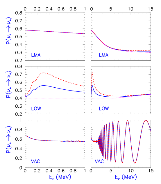
Figure 2: Survival Probabilities. The figure presents the yearly-averaged best-fit survival probabilities determined with strategy (a) for an electron type neutrino that is created in the center of the Sun and arrives at a detector on Earth. The full line refers to the average survival probabilities computed taking into account regeneration in the Earth and the dotted line refers to calculations for the daytime that do not include earth regeneration. The dashed line include regeneration at night. The regeneration effects are computed for the location of the SNO detector for the right hand panels and for the location of the Gran Sasso Underground Laboratory for the left hand panels. There are only slight differences between the computed regeneration effects for detectors located at the positions of SNO, Super-Kamiokande, and Gran Sasso (see ref. [39]). The LOW solutions in the right-hand panel are averaged over a small energy band, $0.1$ MeV, to suppress rapid oscillations caused by a sensitive dependence upon the Earth-Sun distance. The vacuum solutions are averaged over an energy band of $\pm 0.05$ MeV.

2.4 The Predicted Energy and Day-Night Dependence

Figure 2 shows the predicted energy dependence and the day-night asymmetry for the survival probability $P(\nu_{e}\rightarrow\nu_{e})$ of the allowed MSW oscillation solutions, the LMA and LOW solutions, as well as the best-fit vacuum solution.

We plot in figure 2 the best-fit survival probabilities for an electron neutrino that is created in the Sun to remain an electron neutrino upon arrival at a terrestrial detector. The right-hand panels present the survival probability for energies between $0$ and $15$ MeV. The left-hand panels present blow-ups of the behavior of the solutions at energies less than $1$ MeV.

The energy dependence of both MSW solutions is predicted to be very modest above $5$ MeV, in agreement with the fact that no statistically significant distortion of the recoil energy spectrum has yet been observed in the Super-Kamiokande experiment [14]. For the SNO CC measurements, table 2 shows that the expected distortions of the first and second moments of the electron recoil energy spectrum are predicted to be too small to be measurable with statistical significance.

At energies below $5$ MeV, both the LMA and the LOW solutions are predicted to exhibit a significant energy dependence.

At the energies at which water Cherenkov experiments have been possible, the survival probability $P(\nu_{e}\rightarrow\nu_{e})\approx 1/3$, i.e., approximately one over the number of known neutrinos. According to MSW theory, this is an accident. We see from figure 2 that a survival probability of order $0.5$ is predicted for energies less than $1$ MeV.

The day-night asymmetry is potentially detectable for the LMA solution only at energies above $5$ MeV; the predicted asymmetry increases with energy (see figure 2). The situation is just the opposite for the LOW solution. The day-night asymmetry is large below $5$ MeV and relatively small above $5$ MeV.

The vacuum solution has rapid oscillations in energy above $2$ MeV (see figure 2), but these oscillations would be very difficult to observe because they tend to average out over a typical experimental energy bin. At lower energies, the vacuum oscillations will also appear to be smooth, again because of the difficult of resolving in energy the oscillations.

2.5 Analysis details for aficionados: the two-step procedure

The relatively precise values of the CC and NC rates given in the recent SNO paper [1] were extracted by a fit to the observed recoil energy spectrum using the assumption of an undistorted spectrum, i.e. for a survival probability that is constant in energy. These rates cannot be used directly to test an oscillation hypothesis which would cause significant distortions of the CC and ES recoil energy spectra. Since they were aware of the inconsistency in doing so, the SNO collaboration did not use in their oscillation analysis the rates extracted assuming undistorted spectra. Instead, they correctly performed a direct fit to their summed spectrum, including the three contributions from NC, CC and ES (as well as the background) computed for each point in oscillation parameter space.

We include the spectral distortions in a somewhat different way than was done by the SNO collaboration. We perform a two step analysis, which has advantages that we discuss at the end of this section. We use the data generously provided by the SNO collaboration [3].

• First, for a given point in neutrino oscillation parameter space, we compute for each of the $17$ SNO energy bins the oscillation probabilities that are appropriate for evaluating the CC and ES recoil energy spectra. We also compute the number of events that would be expected in each bin for an undistorted energy spectrum (survival probabilities equal to unity everywhere). We multiply the number of events in a given energy bin for the undistorted spectrum by the oscillation probabilities and then add the CC and ES energy spectrum to the NC energy spectrum (which is undistorted). We fit the observed SNO energy spectrum with an arbitrary linear combination of the three energy spectra, CC, ES, and NC, plus the background. The coefficients of the three spectra are evaluated by minimizing the $\chi^{2}$ fit to the observed SNO spectrum. In order to test easily whether the individual results are physically plausible, we normalize the coefficients so that they are unity for an undistorted spectrum. We have verified that the inferred NC, CC, and ES rates are always within the expected physical range. We never encounter unphysical situations: the extracted rates for all three processes, NC, CC, and ES, are always positive and the CC rate never exceeds the NC rate in any part of the parameter space, even in those regions with large spectral distortions. In this way, we obtain as a function of the oscillation parameters, the best-fit CC and NC measured rates (and their corresponding statistical errors, which are strongly anti-correlated).

• Second, with these NC and CC rates, we compute the $\chi^{2}$ for each particular point in oscillation space, combining these two measurements with the available results of all other solar neutrino experiments. We use the three different analysis strategies discussed in ref. [4] and in section 2.1 of this paper. We use for the SNO day-night asymmetry the result quoted for an undistorted spectrum [2], since the small effect of the distortion is expected to nearly cancel out in the asymmetry. In combining the NC and CC data, we take account of the correlation between their errors (both statistical and systematic). We make the approximation that the systematic uncertainties have the same percentage values [1, 2] as they have for the undistorted rates. This approximation is also used, among others, by the SNO collaboration in their recent analysis [2]. In their recent work, Fogli et.al [40] discuss the possible effect of this approximation and find that the approximation is accurate near the local minima but may induce some inaccuracy in the allowed ranges near the boundaries of the $3\sigma$ limits. The results of our full-SNO analysis, presented in section. 5, confirm the conclusion of Fogli et al. We find essentially the same effects as reported by Fogli et al. when we no longer make the assumption that the uncertainties have the same percentage values as are computed for a undistorted spectrum.

  The constraints on the relations between the ES, CC, and NC rates that exist for active oscillations are implemented in step two after the CC and NC extracted rates are included in the global fit together with the ES spectra from Super-Kamiokande. We do not include the SNO ES rate in our global fit, since the Super-Kamiokande ES rate is much more precise, but we do verify, that the extracted SNO ES rate is always compatible with the Super-Kamiokande ES rate.

What are the advantages of the two-step procedure? The most obvious advantage is speed. It is faster to solve for the allowed neutrino oscillation parameters in $\chi^{2}$ space using just the three SNO data points representing the CC and NC fluxes and the day-night difference than it is to solve for the allowed parameters using all $34$ points in the SNO day-night spectrum. Moreover, the use of two distinct methods, the two-step procedure described here and the full-SNO procedure utilized in section 5, permits a test of the robustness of the conclusions. In the two-step procedure, the SNO data are represented by only $3$ data points in the global $\chi^{2}$ (compared to two rate parameters for the radiochemical experiments, chlorine and gallium). Computation of the global $\chi^{2}$ for the full-SNO procedure requires the use of $34$ data points from SNO. Thus for the two-step procedure, SNO is represented in the global $\chi^{2}$ by a comparable number of data points as the radiochemical experiments while in the full-SNO procedure the SNO experiment contributes more than $10$ times as many data points as the radiochemical experiments. Both methods, the two-step procedure and the full-SNO procedure, give (see section 5.2) similar allowed regions and very similar predicted values for solar neutrino observables that will be measured in the future.

Finally, we note that the two-step method has the advantage of transparency. By looking at the computer which contains the coefficients of the NC, CC, and ES energy spectra we can immediately see the effect of any choice of oscillation parameters on the different event rates. This visual inspection also allows us to check quickly for possible unphysical or implausible solutions.

Given that the spectral energy distortions are strongly constrained by the fact that Super-Kamiokande [7, 14] does not observe a significant distortion, it was a priori unlikely that the two methods of taking account of distortions-the two-step procedure and the full-SNO procedure-would lead to significantly different results when analyzing actual solar neutrino experimental data. This expectation is verified quantitatively in section 5.2.

3 Global “Before and After”

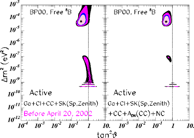
Figure 3: Global “Before and After.” The left panel shows the allowed regions for neutrino oscillations computed using solar neutrino experimental data available prior to April 20 2002. The right panel shows the allowed region computed with the same procedure but including the SNO NC and improved CC data [1] and the SNO day-night asymmetry [2]. In the “Before” panel, the LOW solution is allowed at $97.4$% and in the “After” panel LOW is allowed at the $98.8$%.

What is the impact of the recent SNO measurements [1, 2] on the globally allowed regions of neutrino oscillation parameters?

Figure 3 compares the allowed regions that are found with the solar neutrino data available prior to the presentation of the recent SNO data (i.e., prior to April 20, 2002) with the allowed regions found including the recent SNO data [1, 2]. We like to refer to figure 3 as our “Before and After” figure.

The left panel of figure 3 was computed including the improvements that we described in section 1 regarding the neutrino cross section errors and correlations and the improved average gallium event rate. Hence figure 3a does not correspond to any previously published global oscillation solution, although it could have been computed prior to April 20, 2002.

The recent SNO measurements have greatly shrunk the allowed region for the LOW solution and have significantly reduced the allowed region for the LMA solution, as can be seen by comparing the two panels of figure 3. In particular, maximal mixing is now not allowed at $3\sigma$ and the region does not reach the CHOOZ reactor bound, $\Delta m^{2}\leq 8\times 10^{-4}$ eV²[15].

The LOW solution is now allowed at the $98.8$% CL Before the recent SNO measurements, the LOW solution was allowed at $97.4$%.

4 Predictions for BOREXINO, KamLAND, SNO and a generic $p-p$ detector

We summarize in this section some of the most important predictions that follow from the global neutrino oscillation solutions discussed in section 1 and section 3. To test the robustness of the predictions given in this section, we have calculated the expected values and allowed ranges by two different methods: 1) using the precise values for the CC and NC given in ref. [1] assuming no spectral energy distortions and 2) taking account of the potential effects of spectral energy distortions on the SNO measurements as described in section 2.5. The differences in the calculated values and ranges are negligible in all cases. We present here, for consistency with figure 1 and our previous discussion, the values calculated taking account of the potential spectral distortions in the SNO data.

We summarize in section 4.1 the predictions for the MSW solutions. We answer the following question in section 4.2: How can we distinguish between vacuum and MSW solutions?

4.1 Predictions for MSW solutions

Table 2 presents the best-fit predictions and the expected ranges for none important future solar neutrino observables. The results summarized in table 2 correspond to the right-hand side (the “After” panel) of figure 3. The notation used here is the same as in ref. [4].

Table 2: “After” Predictions. This table presents for future solar neutrino observables the best-fit predictions and $1\sigma$ and $3\sigma$ ranges that were obtained by using analysis strategy (a) and all solar neutrino data currently available. The best-fit values and uncertainties given here correspond to the allowed regions in the right hand panel of figure 3; i.e., this table was constructed by including the data made available by the SNO collaboration on April 20, 2002 [1, 2]. The day-night asymmetries for the SNO and the ⁷Be (BOREXINO) experiments are denoted by $A_{\rm N-D}$ and are defined by eq. (9). The reduced ⁷Be, $p-p$, and ⁸B event rates are defined by eq. (10) and eq. (11); the reduced KamLAND CC rate is defined by eq. (12). The first moment of the recoil electron energy distribution is denoted by $\delta T$ for SNO and $\delta E_{\rm visible}$ for KamLAND; the second moments are denoted by $\delta\sigma$. The threshold of the recoil electron kinetic energy used in computing the SNO observables for this table is $5$ MeV. For the BOREXINO experiment, we consider electron recoil energies between between $0.25~{}{\rm MeV}$ and $0.8~{}{\rm MeV}$ (see ref. [16]). We present the results for the KamLAND reactor observables for two thresholds, $E_{\rm th}=1.22$ and 2.72 MeV.

Observable	b.f. $\pm 1\sigma$	LMA $\pm 3\sigma$	LOW $\pm 3\sigma$
AN-D (SNO CC) (%)	$5.2^{+3.6}_{-3.5}$	$5.2^{+9.3}_{-5.2}$	$2.7^{+2.7}_{-2.1}$
$\delta T$ (SNO CC) (%)	$-0.17^{+0.19}_{-0.56}$	$-0.17^{+0.31}_{-1.55}$	$0.42^{+0.55}_{-0.35}$
$\delta\sigma$ (SNO CC) (%)	$0.03^{+0.17}_{-0.61}$	$0.03^{+0.25}_{-1.77}$	$0.52^{+0.66}_{-0.44}$
$[$R (7Be)$]$ $\nu-e$ scattering	$0.64\pm 0.03$	$0.64^{+0.09}_{-0.05}$	$0.58\pm 0.05$
AN-D (7Be) (%)	$0.0^{+0.0}_{-0.0}$	$0.0^{+0.1}_{-0.0}$	$23^{+10}_{-13}$
$[$R (8B)$]$ $\nu-e$ scattering
($T_{\rm th}=3.5$ MeV)	$0.46\pm 0.03$	$0.46\pm 0.04$	$0.46\pm 0.03$
($T_{\rm th}=5$ MeV)	$0.46\pm 0.03$	$0.46\pm 0.04$	$0.46\pm 0.03$
$[$CC$]$ (KamLAND)
($E_{\rm th}=2.72$ MeV)	$0.49^{+0.20}_{-0.17}$	$0.49^{+0.25}_{-0.26}$	—
($E_{\rm th}=1.22$ MeV)	$0.52\pm 0.15$	$0.52^{+0.20}_{-0.25}$	—
$\delta E_{\rm visible}$ (KamLAND) (%)
($E_{\rm th}=2.72$ MeV)	$-7^{+13}_{-2}$	$-7^{+14}_{-4}$	—
($E_{\rm th}=1.22$ MeV)	$-9^{+13}_{-3}$	$-9^{+17}_{-5}$	—
$\delta\sigma$ (KamLAND)(%)
($E_{\rm th}=2.72$ MeV)	$-5^{+11}_{-10}$	$-5^{+20}_{-14}$	—
($E_{\rm th}=1.22$ MeV)	$-8^{+20}_{-8}$	$-8^{+26}_{-12}$	—
$[p$-$p]$ $\nu-e$ scattering
($T_{\rm th}=100$ keV)	$0.705^{+0.031}_{-0.026}$	$0.705^{+0.073}_{-0.049}$	$0.683^{+0.035}_{-0.042}$
($T_{\rm th}=50$ keV)	$0.700^{+0.031}_{-0.027}$	$0.700^{+0.074}_{-0.050}$	$0.677^{+0.038}_{-0.045}$

How much of a difference have the recent SNO measurements made in the expected values for future solar neutrino observables? The reader can answer this question by comparing table 3 with table 2 . Here, table 3 presents the best-fit predictions and allowed ranges that correspond to using solar neutrino data available prior to April 20, 20002. In particular, the values given in table 3 were obtained using the global solution shown in the left-hand side, the “Before” panel, of figure 3.

The principal differences between the results summarized in table 2 and table 3 are a consequence of the smaller allowed region of the LOW solution shown in the “After” panel of figure 3. The changes that result from the modest reduction of the LMA allowed region are generally not very significant.

The predicted day-night asymmetries, $A_{\rm N-D}$, between the nighttime and the daytime event rates for SNO and for BOREXINO (⁷Be $\nu-e$ scattering detector) are given in the first and third rows, respectively, of table 2 and table 3. The results presented correspond to an average over one year. The definition of $A_{\rm N-D}$ is

$$A_{\rm N-D}~{}=~{}2{\rm{[Night-Day]}\over{[Night+Day]}}~{}.$$ (9)

We have used $1$ km steps ($6371$ total points) to compute the values for the day-night effect in the SNO CC measurement. Compared to the results obtained using a cruder grid of $50$ km steps, the best-fit values for the $A_{N-D}$ for the LMA are shifted up by $\sim 10$%. The LOW predictions for $A_{N-D}$ are not significantly affected. The main reason for that shift in the values calculated for the LMA is the more accurate parameterization of the PREM density [41] of the earth in the external shells.

The minimum predicted value for the LOW day-night asymmetry, A_N-D (⁷Be), in BOREXINO is now a whopping-big $10$% at $3\sigma$. Prior to April 20, 2002, a $0$% value of A_N-D (⁷Be) was allowed even for the LOW solution. There are no significant differences in the Before and After predictions for the SNO CC value of A_N-D.

The first and second moments of the SNO CC spectrum for the case of no oscillations are $\langle T_{0}\rangle=7.74$MeV and $\langle\sigma_{0}\rangle=1.87$ MeV. The range of predicted shifts with respect to these no-oscillation values is always smaller than $\sim 2$% within both the LMA and LOW $3\sigma$ regions and is not significantly different from the range found in the “Before” analysis. Larger shifts for the moment second moment ($7$%) are possible within the allowed VAC oscillation region. The non-statistical uncertainties in measuring the first and second moments in SNO have been estimated, prior to the operation of the experiment, in ref. [42] and are, respectively, about $1$% and $2$%.

Table 3: “Before” Predictions. This table presents for future solar neutrino observables the best-fit predictions and $1\sigma$ and $3\sigma$ ranges that were obtained by using analysis strategy (a) and solar neutrino data available before April 20, 2002. The best-fit and uncertainties given here correspond to the allowed regions in the left hand panel of figure 3. The format and procedures used in constructing this table are the same as used in constructing table 2 except that here we have not included the recent SNO data [1, 2].

Observable	b.f. $\pm 1\sigma$	LMA $\pm 3\sigma$	LOW $\pm 3\sigma$
AN-D (SNO CC) (%)	$4.9^{+4.1}_{-3.4}$	$4.9^{+11.7}_{-4.9}$	$1.3^{+3.9}_{-1.3}$
$\delta T$ (SNO CC) (%)	$-0.23^{+0.25}_{-0.57}$	$-0.23^{+0.39}_{-1.58}$	$0.25^{+0.71}_{-0.44}$
$\delta\sigma$ (SNO CC) (%)	$0.16^{+0.12}_{-0.78}$	$0.16^{+0.13}_{-2.0}$	$0.25^{+0.96}_{-1.02}$
$[$R (7Be)$]$ $\nu-e$ scattering	$0.66\pm 0.04$	$0.66^{+0.09}_{-0.07}$	$0.59^{+0.13}_{-0.06}$
AN-D (7Be) (%)	—	$0.0^{+0.1}_{-0.0}$	$15^{+17}_{-15}$
$[$R (8B)$]$ $\nu-e$ scattering
($T_{\rm th}=3.5$ MeV)	$0.46\pm 0.03$	$0.46\pm 0.04$	$0.45\pm 0.03$
($T_{\rm th}=5$ MeV)	$0.46\pm 0.03$	$0.46\pm 0.04$	$0.45\pm 0.03$
$[$CC$]$ (KamLAND)
($E_{\rm th}=2.72$ MeV)	$0.56^{+0.14}_{-0.22}$	$0.56^{+0.20}_{-0.34}$	—
($E_{\rm th}=1.22$ MeV)	$0.57^{+0.1}_{-0.18}$	$0.57^{+0.16}_{-0.31}$	—
$\delta E_{\rm visible}$ (KamLAND) (%)
($E_{\rm th}=2.72$ MeV)	$-7^{+12}_{-2}$	$-7^{+14}_{-4}$	—
($E_{\rm th}=1.22$ MeV)	$-7^{+11}_{-4}$	$-7^{+15}_{-7}$	—
$\delta\sigma$ (KamLAND) (%)
($E_{\rm th}=2.72$ MeV)	$-6^{+16}_{-9}$	$-6^{+21}_{-12}$	—
($E_{\rm th}=1.22$ MeV)	$-9^{+19}_{-7}$	$-9^{+28}_{-11}$	—
$[p$-$p]$ $\nu-e$ scattering
($T_{\rm th}=100$ keV)	$0.722^{+0.033}_{-0.042}$	$0.722^{+0.085}_{-0.067}$	$0.689^{+0.058}_{-0.065}$
($T_{\rm th}=50$ keV)	$0.718^{+0.034}_{-0.043}$	$0.718^{+0.086}_{-0.069}$	$0.687^{+0.058}_{-0.068}$

Based upon the results given in table 2, we predict that SNO will not measure a statistically significant ($>3\sigma$) distortion to the recoil energy spectrum for the CC reaction. This prediction constitutes an important consistency test of the oscillation analysis and the understanding of systematic effects in the detector.

The prediction for the reduced ⁷Be $\nu-e$ scattering rate,

$$[{\rm{}^{7}Be}]~{}\equiv~{}\frac{\rm Observed~{}\nu-e~{}scattering~{}rate}{\rm BP00~{}predicted~{}rate}~{},$$ (10)

is remarkably precise and remarkably stable. The current prediction for what BOREXINO will measure if the LMA solution is valid is $[{\rm{}^{7}Be}]=0.64^{+0.04}_{-0.03}$. A somewhat smaller value is predicted if the LOW solution is correct.

We have also evaluated the predictions for a generic $p-p$ neutrino-electron scattering detector. The reduced rate for this detector is defined, analogously to the reduced rate for ⁷Be detectors, by the relation

$$[p-p]~{}\equiv~{}\frac{\rm Observed~{}\nu-e~{}scattering~{}rate}{\rm BP00~{}predicted~{}rate}~{}.$$ (11)

We present the predicted rate for two plausible kinetic energy thresholds, $100$ keV and $50$ keV. The predicted rate is precise and robust, which supports previous suggestions that a measurement of the $p-p$ neutrino scattering rate can be used to determine accurately the dominant solar neutrino mixing angle.

We also include in table 2 the predictions for the expected $\nu-e$ scattering rate, [R(⁸B)] (defined similarly to [⁷Be] and [$p-p$]), from ${}^{8}B$ neutrinos above two different electron recoil kimetic-energy energy thresholds, $T_{\rm th}=3.5$ MeV and $T_{\rm th}=5$ MeV. The rates expected if the LMA or LOW solution is correct are essentially identical to the neutrino-electron scattering rates measured at higher thresholds by the SNO and Super-Kamiokande collaborations, which are $0.47\pm 0.13$ and $0.46\pm 0.04$, respectively (relative to the value predicted with the BP00 standard solar model flux). Thus a measurement of the ⁸B $\nu-e$ scattering rate in BOREXINO, or with a low threshold in Super-Kamiokande, is not expected to yield a significant deviation from the rate measured at higher energies.

The predicted value of the reduced CC event rate in the KamLAND reactor experiment,

$$[{\rm CC}]({\rm KamLAND})~{}\equiv~{}\frac{\rm Observed~{}\bar{\nu}+p~{}absorption~{}rate}{\rm No~{}oscillation~{}rate}~{},$$ (12)

is not significantly affected by the recent SNO results. The best-fit prediction shifts slightly (to a lower value) but the shift is well-within the $1\sigma$ currently allowed range.

For KamLAND, it is convenient to represent the distortion of the visible energy spectrum by the fractional deviation from the undistorted spectrum of the first two moments of the energy spectrum. We follow the notation and analysis of refs. [4, 42, 43]. The predicted fractional distortion of the first two moments is not significantly affected by the recent SNO measurements. Since table 2 and table 3 give only the fractional changes of the moments relative to the moments for the undistorted spectrum, we must also specify the values calculated for a spectrum unaffected by new physics. In the absence of oscillations, one expects [4]: $\langle E_{\rm vis}\rangle_{0}=3.97$ MeV and $\langle\sigma\rangle_{0}=1.26$ MeV for $E_{\rm threshold}=1.22$ MeV ($\langle E_{vis}\rangle_{0}=4.33$ MeV and $\langle\sigma\rangle_{0}=1.06$ MeV for $E_{\rm threshold}=1.72$ MeV).

4.2 Predictions for vacuum solutions

The clearest evidence against the vacuum oscillations would be the observation of a rate depletion or a spectral distortion in the KamLAND reactor experiment. The $\Delta m^{2}$ for vacuum oscillations is too small to lead to an observable effect with KamLAND.

Within the $3\sigma$ allowed VAC regions, the distortion of the SNO spectrum corresponds to a shift in the first (second) moment of the recoil energy distribution of at most -2% (+6%) and no significant seasonal variation at SNO is expected. The predicted ⁷Be rate for vacuum oscillations at BOREXINO is in the same range as the predictions for LMA and LOW solutions. The most striking signal for vacuum oscillations would be the observation of a large seasonal variation in the BOREXINO experiment, with a clear pattern of the monthly dependence of the observed rate [44]. There should also be a day-night effect at BOREXINO associated with this seasonal variation; the day-night asymmetry should be at most $\pm 8$% (the size and sign of this asymmetry is sensitive to the exact value of $\Delta m^{2}$ considered to be within the allowed VAC islands) due to the dependence of the survival probability upon the earth-sun distance.

Figure 4: Global neutrino oscillation solutions with full SNO day-night spectrum and analysis strategy (a). To assess the robustness of the global oscillation solutions, compare this figure with figure 1a or 3b. The input data used in constructing figure 4 include the SNO day-night spectrum  [2], the Chlorine [10] and Gallium (averaged) [6, 11, 12, 13] event rates, as well as the zenith angle-recoil energy spectrum data presented by Super-Kamiokande [14] and the neutrino fluxes and uncertainties predicted by the standard solar model [8] except for the ⁸B flux (which is treated as a free parameter). The rates from the GALLEX/GNO and SAGE experiments have been averaged to provide a unique data point ($72.4\pm 4.7$ SNU). The CL contours shown in the figure are $90$%, $95$%, $99$%, and $99.73$% ($3\sigma$). The global best-fit points are marked by a star.

5 Global analysis including the full SNO day-night energy spectrum

In order to help determine the robustness of the oscillation solutions found in section 2, we have recalculated the global solutions using the full SNO day-night energy spectrum instead of the two step treatment of SNO data described in section 2.5. This full-SNO procedure has been used, by among others, the SNO collaboration [2].

We begin by presenting in section 5.1 the global solutions obtained using the full SNO analysis procedure and then compare in section 5.2 the allowed ranges for $\Delta m^{2}$, $\tan^{2}\theta$, and $f_{\rm B}$ found by the two step procedure and the inclusion of the full SNO day-night energy spectrum. We compare in section 5.3 the predictions for future measurements with the BOREXINO, KamLAND, and SNO detectors and a generic future $p-p$ solar neutrino detector. We describe in section 5.4 details of the analysis procedure, details that are probably only of interest to aficionados.

5.1 Global solutions

Figure 4 presents the result of our ”full-SNO” global analysis (strategy a) that was obtained using the full SNO day-night energy spectrum in combination with the Super-Kamiokande zenith-angle energy spectrum and the Ga and Cl event rates. The number of degrees of freedom in this analysis is 77: 44 (Super-Kamiokande zenith-angle energy spectrum) + 2 (Ga and Cl rates) + 34 (SNO day-night energy spectrum) $-$3 parameters ( $\Delta{\rm m}^{2}$, $\theta$, and $f_{\rm B}$).

To simplify the comparison with our results obtained with the two-step analysis of the SNO data (see figure 1 and figure 3b), we continue to use the average gallium rate $72.4\pm 4.7$ SNU and do not include the recent, preliminary GNO data reported at Neutrino 2002 (which would result into a slight lowering of the rate to $70.8\pm 4.4$ SNU). We have verified that the use of this lower rate would not affect significantly any of the conclusions of the present analysis. The $\chi^{2}$ value for LMA would be lowered by $+0.3$, while the difference between LMA and LOW (and VAC) solutions is decreased by $0.3$.

Table 4: Best-fit global oscillation parameters obtained using the full SNO day-night energy spectrum. The values given here, which were computed using the full SNO day-night energy spectrum, should be compared with the values given in table 1, which were computed using the two-step treatment of SNO data that is described in section 2.5. Table 4 gives the best-fit values for $\Delta m^{2}$, $\tan^{2}\theta$, $\chi^{2}_{\rm min}$, and g.o.f. for all the oscillation solutions among active solar neutrinos that have been previously discussed (see, e.g., ref. [21]). The quantity $f_{\rm B}$ measures the ⁸B solar neutrino flux in units of the predicted BP00 neutrino flux, see eq. (5). The oscillation solutions are obtained by varying the ⁸B flux as free parameter in a consistent way: simultaneously in the rates and in the fits to the night and day energy spectra. The differences of the squared masses are given in ${\rm eV^{2}}$. The number of degrees of freedom is is 77 [44 (Super-Kamiokande zenith-angle energy spectrum) + 2 (Ga and Cl event rates) + 34 (SNO day-night energy spectrum) $-$3 (parameters: $\Delta{\rm m}^{2}$, $\theta$, and $f_{\rm B}$)]. The goodness-of-fit given in the last column is calculated relative to the minimum for each solution. (Solutions that have $\chi_{\rm min}^{2}\geq 75.4+11.8=87.2$ are not allowed at the $3\sigma$ CL)

Solution	$\Delta m^{2}$	$\tan^{2}(\theta)$	$f_{\rm B,best}$	$\chi^{2}_{\rm min}$	g.o.f.
LMA	$5.8\times 10^{-5}$	$4.5\times 10^{-1}$	1.02	75.4	$53$%
LOW	$7.9\times 10^{-8}$	$6.3\times 10^{-1}$	0.93	85.0	$25$%
VAC	$6.5\times 10^{-10}$	$1.5\times 10^{0}$	0.76	85.5	$23$%
SMA	$4.7\times 10^{-6}$	$1.7\times 10^{-3}$	0.92	101.0	$3.4$%
Just So2	$5.8\times 10^{-12}$	$1.0\times 10^{0}$	0.45	115.1	$0.3$%
Sterile VAC	$4.5\times 10^{-10}$	$2.5\times 10^{0}$	0.78	101.4	$3.3$%
Sterile Just So2	$5.8\times 10^{-12}$	$1.0\times 10^{0}$	0.45	111.8	$0.6$%
Sterile SMA	$3.6\times 10^{-6}$	$4.2\times 10^{-4}$	0.55	115.1	$0.3$%

5.2 Comparison of two-step and full-SNO analysis procedures

Table 4 gives, for our full-SNO global analysis (cf. figure 4), the best-fit values for $\Delta m^{2}$ and $\tan^{2}\theta$ for all the neutrino oscillation solutions. The table also lists the values of $\chi_{\rm min}^{2}$ for each solution. The regions for which the local value of $\chi_{\rm min}^{2}$ exceeds the global minimum by more than $11.83$ are not allowed at $3\sigma$ CL.

Comparing the right hand panel of figure 3 with figure 4 and the corresponding minima in table  1 with those in table 4 shows that the main effect of the inclusion of the full day-night spectrum information is, as expected, the moderate worsening of solutions with larger spectrum distortions. SMA becomes even further disfavored (acceptable only at the $4.7\sigma$ CL) while vacuum solutions are now only marginally allowed at 3$\sigma$ (acceptable at the $2.7\sigma$ CL). Furthermore, the best-fit vacuum solution is moved into the second lowest $\Delta m^{2}$ island. The confidence level for the LOW solution exceeds $99$% CL (acceptable at the $2.6\sigma$ CL).

How are the ranges of allowed masses and mixing changed?

In units of ${\rm eV^{2}}$, we find for the LMA solution the following $3\sigma$ limits on $\Delta m^{2}$,

$$2.4\times 10^{-5}<\Delta m^{2}<4.7\times 10^{-4}.$$ (13)

For the LOW solution, the allowed mass range is

$$3.2\times 10^{-8}<\Delta m^{2}<1.1\times 10^{-7}.$$ (14)

Comparing these results with the corresponding results given in eq. 1 and eq. 2 for the two-step procedure for analyzing SNO data, we see that in both cases the full-SNO procedure gives a slightly larger $3\sigma$ range for $\Delta m^{2}$.

The allowed range for the LMA mixing angle is

$$0.27<\tan^{2}\theta<0.92$$ (15)

and for the LOW solution

$$0.47<\tan^{2}\theta<0.89$$ (16)

Comparing the limits given above with the values found earlier (see eq. 3 and eq. 4) using the two-step procedure, we conclude that the full-SNO procedure gives a slightly shifted $3\sigma$ range for $\tan^{2}\theta$.

For the global solution shown in figure 4, the $1\sigma[3\sigma]$ allowed range of $f_{\rm B}$ is

$$f_{\rm B}~{}=~{}1.02\pm 0.08~{}({1\sigma})~{}~{}[f_{\rm B}~{}=~{}1.02\pm{0.24}]~{}({3\sigma})~{}({\rm LMA}).$$ (17)

The range of $f_{\rm B}$ was calculated, as just as it was for eq .(7) and eq. (8), by marginalizing over the full space of oscillation parameters ($\Delta m^{2}$, $\tan^{2}2\theta$). Hence we use $\Delta\chi^{2}$ conditions for 1 dof, relative to the global minimum value for $\chi^{2}$ that lies in the LMA allowed region. Since for the full-SNO analysis procedure $\Delta\chi^{2}=\chi^{2}_{\rm LOW}-\chi^{2}_{\rm LMA}>9$, there are no allowed solutions for $f_{\rm B}$ at the $3\sigma$ CL ($1$ dof) within either the LOW or vacuum solution domains.

The uncertainties shown in eq. 17 are essentially the same as the uncertainties in $f_{\rm B}$ that were found using the two-step procedure for analyzing SNO data (see eq .7 and eq. 8). We conclude that the uncertainties in all three of the parameters $\Delta m^{2}$, $\tan^{2}\theta$, and $f_{\rm B}$ are robust with respect to the choice of analysis procedures for the SNO data.

5.3 Predictions for BOREXINO, KamLAND, SNO and a generic $p-p$ detector

The predicted event rates for measurable solar neutrino quantities are essentially the same if one uses the full-SNO day-day night energy spectrum or if one uses the two-step procedure.

Table 5 gives the predicted ranges for future solar neutrino observables that correspond to the allowed regions in figure 4. The values shown in table 5 should be compared with the results presented in table 2, which was obtained using the two-step procedure for SNO data. The comparison shows that there are small shifts in some of the central values of the observables due to the slight shifts in the positions of the LMA and LOW best fit points. However, the predicted ranges are not significantly modified.

Table 5: “After” Predictions obtained using the full SNO day-night energy spectrum. This table presents for future solar neutrino observables the best-fit predictions and $1\sigma$ and $3\sigma$ ranges that were obtained by using the analysis including the SNO day-night spectrum and all other solar neutrino data currently available. The best-fit values and uncertainties given here correspond to the allowed regions in the figure 4. The predictions given in this table should be compared with table 2, which was obtained by treating the SNO data by the two-step procedure described in section 2.5.

Observable	b.f. $\pm 1\sigma$	LMA $\pm 3\sigma$	LOW $\pm 3\sigma$
AN-D (SNO CC) (%)	$4.2^{+3.8}_{-2.9}$	$4.2^{+8.9}_{-4.2}$	$2.7^{+2.2}_{-2.2}$
$\delta T$ (SNO CC) (%)	$-0.10^{+0.30}_{-0.50}$	$-0.10^{+0.38}_{-1.64}$	$0.46^{+0.52}_{-0.41}$
$\delta\sigma$ (SNO CC) (%)	$-0.25^{+0.28}_{-0.50}$	$0.25^{+0.39}_{-1.46}$	$0.38^{+0.42}_{-0.33}$
$[$R (7Be)$]$ $\nu-e$ scattering	$0.64\pm 0.03$	$0.64^{+0.09}_{-0.05}$	$0.59\pm 0.04$
AN-D (7Be) (%)	$0.0^{+0.0}_{-0.0}$	$0.0^{+0.1}_{-0.0}$	$23^{+9}_{-13}$
$[$R (8B)$]$ $\nu-e$ scattering
($T_{\rm th}=3.5$ MeV)	$0.46\pm 0.03$	$0.46\pm 0.04$	$0.45\pm 0.03$
($T_{\rm th}=5$ MeV)	$0.45\pm 0.03$	$0.45\pm 0.04$	$0.45\pm 0.03$
$[$CC$]$ (KamLAND)
($E_{\rm th}=2.72$ MeV)	$0.58^{+0.10}_{-0.27}$	$0.58^{+0.14}_{-0.35}$	—
($E_{\rm th}=1.22$ MeV)	$0.57^{+0.08}_{-0.20}$	$0.57^{+0.12}_{-0.30}$	—
$\delta E_{\rm visible}$ (KamLAND) (%)
($E_{\rm th}=2.72$ MeV)	$-7^{+13}_{-2}$	$-7^{+14}_{-4}$	—
($E_{\rm th}=1.22$ MeV)	$-5^{+10}_{-5}$	$-5^{+13}_{-8}$	—
$\delta\sigma$ (KamLAND) (%)
($E_{\rm th}=2.72$ MeV)	$-11^{+23}_{-4}$	$-11^{+26}_{-7}$	—
($E_{\rm th}=1.22$ MeV)	$-14^{+24}_{-3}$	$-14^{+32}_{-6}$	—
$[p$-$p]$ $\nu-e$ scattering
($T_{\rm th}=100$ keV)	$0.699^{+0.026}_{-0.025}$	$0.699^{+0.069}_{-0.044}$	$0.686^{+0.033}_{-0.034}$
($T_{\rm th}=50$ keV)	$0.695^{+0.026}_{-0.025}$	$0.695^{+0.070}_{-0.045}$	$0.681^{+0.035}_{-0.037}$

5.4 Analysis details for aficionados: using the full SNO day-night energy spectrum

We describe in this subsection the details of our analysis procedure when we include the full SNO day-night energy spectrum. We perform a direct fit to the total SNO day-night energy spectrum, including contributions from NC, CC, and ES events.

In order to avoid redundancy with the discussion in section 2.5, we also provide in this section some detailed information about analysis procedures and error estimates that is necessary for comparing our results with the results obtained by other analysis groups. This additional information is relevant to both the two-step and the full-SNO analysis procedures.

We use the detailed information provided in ref. [3] by the SNO collaboration. For each point in oscillation parameter space, we compute (as with the two-step procedure) the expected event rates for the chlorine and gallium experiments, and the Super-Kamiokande zenith-angle energy spectrum. For the SNO day-night energy spectrum, we compute the NC, CC, and ES contributions in each energy bin. We construct a theoretical SNO spectrum by summing the NC, CC, and ES contributions together with the background rates given in ref. [3]. With these model predictions, we make a global fit including as the $80$ data points, the $2$ radio-chemical rates, the $44$ data points of the Super-Kamiokande zenith-angle spectrum, and the $34$ points of the SNO day-night spectrum.

We include the errors and their correlations for all of these observables. We construct an $80\times 80$ covariance error matrix that includes the effect of correlations between the different errors as off diagonal elements (an alternative “pull” method has been recently proposed in ref. [40]). The main sources of correlations are due to the BP00 neutrino fluxes, the cross section uncertainties for the gallium and chlorine rates, and the cross sections and experimental systematic errors for Super-Kamiokande and SNO energy spectra. As in our two-step analysis, the flux and cross section errors are included following the general approach described in ref. [30] with the refinements described in the appendix of ref. [5].

The experimental systematic errors can be either correlated or uncorrelated in energy. We include these errors as follows . For Super-Kamiokande, we take from table $1$ of ref. [7] the systematic error, which we include as uncorrelated among the Super-Kamiokande energy bins but fully correlated among the zenith-angle bins. For SNO, energy independent but correlated errors include the systematic errors from the uncertainty in vertex reconstruction ($+3$% for CC and ES and +$1.45$% for NC), the background errors from neutron capture, and low-energy correlated systematic uncertainties. Each of these errors are fully correlated among the $34$ SNO bins. Furthermore, the fractional error is assumed to be constant, i.e. independent (in %) of the oscillation point and affecting equally ⁸B and hep neutrinos.

For both Super-Kamiokande and SNO there also energy-dependent and energy-correlated errors from (i) the ⁸B spectral energy shape, (ii) the absolute energy scale, and (iii) the energy resolution. The fractional value of those errors is, in general, affected by distortions of the spectrum due to oscillations and therefore they should be evaluated for each point in the oscillation parameter space. The Super-Kamiokande and the SNO collaborations do not specify the details of what they use for these errors. We evaluate the three errors listed above as follows. First, we compute for each point in oscillation parameter space the expected number of ES events in each energy bin for the Super-Kamiokande spectrum, and the number of CC, ES, and NC events in each energy bin for SNO. We then evaluate the fractional change in the calculated results by: (i) shifting the normalization of the ⁸B spectrum up and down within the 1$\sigma$ error determined in ref. [45] in order to obtain the error associated with the ⁸B spectrum shape; (ii) shifting the calibrated energy $T^{\prime}$ to $T^{\prime}(1\pm\delta_{T})$ with $\delta T=0.64$% (1.21%) for Super-Kamiokande (SNO) to obtain the error associated with the energy scale; (iii) sifting the width of the resolution function $\sigma$ to $\sigma(1\pm\delta_{\sigma})$ with $\delta_{\sigma}=0.025$ for Super-Kamiokande($\delta_{\sigma}=0.045+0.004\times(T-4.98)$ for SNO) to obtain the error due to the energy resolution. Whenever a comparison was possible, we have verified that the error estimates made as described above are in good agreement with the information about the errors that has been provided by the Super-Kamiokande and SNO collaborations. Each of these errors is fully correlated among the different bins in each experiment. Moreover, the shape errors are also correlated between the Super-Kamiokande and SNO experiments.

6 Discussion and summary

In the following, we present without parentheses results that were obtained by the two-step procedure for analyzing SNO data (and present in parentheses the corresponding results that were obtained by analyzing the full SNO day-night energy spectrum). If the results are identical for both treatments of the SNO data, then we omit the value in parenthesis. By comparing the values given with and without parentheses, the reader can see the rather small differences that result from different choices of how to treat the SNO data.

Figure 1 and figure 3, together with table 1 (or, alternatively, figure 4 and table 4), tell much of the story. These global analyses, which use all the available solar neutrino data, demonstrate that only large mixing angle solutions are currently allowed at the $3.7\sigma$ ($4.7\sigma$) confidence level. We therefore know at an impressive confidence level that there are relatively large mixing angles for oscillations between solar neutrinos (and between atmospheric neutrinos), unlike the small mixing angles among quarks. However, precise maximal mixing is excluded at $3.2\sigma$ for MSW solutions [see eq. 3 and eq. 4 (eq. 15 and eq. 16) for the exact allowed regions] and at $2.8\sigma$ ($2.9\sigma$) for vacuum oscillations. The masses and mixing angles for solar neutrinos do not appear to satisfy an obviously simple pattern.

Among the MSW solutions, the situation has also been clarified. The LMA solution is now the only viable solution at a level of $2.5\sigma$ (2.6 $\sigma$). The LOW solution is excluded at the $98.8$% ($99.2$%) CL. The KamLAND and BOREXINO experiments will test strongly this conclusion. The SMA solution is now excluded at more than $3.7\sigma$ (4.7 $\sigma$). Pure sterile oscillations are excluded at $5.4\sigma$ (4.7 $\sigma$).

The possibility of a strictly energy independent solution of the solar neutrino problem is excluded at more than $3.6\sigma$. If we consider solutions that have an energy variation less than $10$% over the energy range of interest, the exclusion is at more than $2.6\sigma$. We note that such a weak energy dependence can probably not be distinguished experimentally from strict energy independence (see ref. [46] for details).

Vacuum solutions are not favored, but are acceptable at $2.1\sigma$ ($2.7\sigma$).

Table 6: Neutrino oscillation predictions for the chlorine and gallium radiochemical experiments. The predictions are based upon the global analysis strategy (a), and use the neutrino fluxes for the BP00 standard solar model (except for the ⁸B flux for which the factor $f_{\rm B}$ is included) and the neutrino absorption cross sections [49, 45, 47]. The rates are presented for the best-fit oscillation parameters of the allowed solutions listed in table 1. The total rates should be compared with the standard solar model values [8], which are, $7.6^{+1.3}_{-1.1}$ (chlorine) and $128^{+9}_{-7}$(gallium), and the measured values, which are $2.56\pm 0.23$ (chlorine [10]) and $72.4\pm 4.7$(gallium [6, 11, 12]. )

Source	Cl	Ga	Cl	Ga	Cl	Ga
	(SNU)	(SNU)	(SNU)	(SNU)	(SNU)	(SNU)
	LMA	LMA	LOW	LOW	VAC	VAC
pp	0	40.4	0	38.2	0	40.3
pep	0.12	1.51	0.10	1.25	0.15	1.82
hep	0.01	0.02	0.02	0.03	0.02	0.04
${\rm{}^{7}Be}$	0.62	18.6	0.53	16.0	0.46	14.0
${\rm{}^{8}B}$	2.05	4.35	2.26	4.72	2.34	5.00
${\rm{}^{13}N}$	0.04	1.79	0.04	1.56	0.05	1.83
${\rm{}^{15}O}$	0.15	2.83	0.15	2.44	0.18	3.01
${\rm{}^{17}F}$	0.00	0.03	0.00	0.03	0.00	0.04
Total	$3.03$	$69.6$	$3.11$	$64.2$	$3.21$	$66.0$

For the reader who (like us) often prefers pictures to tables, figure 2 shows the predicted energy dependence and day-night difference for the current best-fit LMA, LOW, and VAC solutions.

The global oscillation solutions constrain the active ⁸B solar neutrino flux with somewhat greater accuracy than the SNO NC measurement. The accuracy of the SNO NC measurement is $\pm 12$% [1]. We find from a global oscillation solution of all the data, that at the $1\sigma$ CL, $f_{\rm B}~{}=~{}1.07\pm 0.08$ ($f_{\rm B}~{}=~{}1.02\pm 0.08$), where $f_{\rm B}$ is the total flux of active ⁸B solar neutrinos in units of the flux predicted by the standard solar model [8]. The allowed ranges of $f_{\rm B}$ for the LMA and LOW solutions are given in eq. (7) and eq. (8) (eq. 17) at $1\sigma$ and $3\sigma$ CL.

We have calculated the predicted best-fit values and allowed ranges for ten important solar neutrino observables for the BOREXINO, KamLAND, and SNO experiments and for a generic detector of $\nu-e$ scattering by $p-p$ neutrinos. The observables include total rates, day-night effects, and spectral distortions. The predictions are summarized in the “Before” and “After” tables, table 2 and table 3, and in section 4.2. Similar results are presented for the full-SNO procedure in table (5) and in section 5.3. The predictions are rather robust and are not significantly affected by the choice of procedure (two-step or full-SNO) used to analyze the SNO data. Only the predictions for the disfavored LOW solution are significantly affected by the recent SNO measurements [1, 2]. We have also calculated the predicted values and ranges given in table 2 and table 3 both with and without taking account of potential spectral energy distortions in interpreting the SNO data (see section 2.5 and ref. [3]). Both methods give essentially identical results.

For completeness, table 6 gives the individual contributions of different solar neutrino sources to the predicted event rates for the chlorine and gallium experiments. The results presented in table 6 were obtained using the best-fit oscillation solutions of table 1. The values given in the table were calculated with the two-step treatment of the SNO data. The calculated chlorine and gallium rates are essentially the same when the best-fit solutions are used that were obtained including the full SNO day-night energy spectrum. In that case, the predicted rates for the LMA solution are increased by about $1$% and the predicted values for the LOW and vacuum solutions are decreased by between $2$% and $7$%. The rates shown in table 6 are also very similar to the rates that were expected [4] prior to the recent SNO measurements.

The most important next generation solar neutrino experiment will detect the fundamental $p$-$p$ neutrinos, which constitute $91$% of the total neutrino flux predicted by the BP00 solar model. Unfortunately, there are no approved $p$-$p$ solar neutrino experiments at the present time, although there are a number of very promising proposals under development. Among the CC detectors, only LENS  [50] is in a advanced stage of research development and even for LENS important details regarding the detector are not yet known. There are a number of potential $\nu-e$ scattering experiments [51] that could observe $p$-$p$ neutrinos. Therefore, for completeness we have added the predictions for a generic $\nu-e$ scattering experiment using $p$-$p$ neutrinos. Table 2 and table 3 (see also table 5) give the calculated values of the $p-p$ $\nu-e$ scattering rate for two plausible recoil electron kinetic energy thresholds, $50$ keV and $100$ keV.

We are grateful to the SNO collaboration for the thrill of analyzing solar neutrino data that include a neutral current measurement. We have profited from several discussions with M. Chen, F. Duncan, and A. McDonald regarding the analysis methods used by the SNO collaboration and from a constructive referee’s report. JNB acknowledges support from NSF grant No. PHY0070928. MCG-G is supported by the European Union Marie-Curie fellowship HPMF-CT-2000-00516. This work was also supported by the Spanish DGICYT under grants PB98-0693 and FPA2001-3031.

References

- [1] SNO collaboration, Q.R. Ahmad et al., Direct evidence for neutrino flavor transformation from neutral-current interactions in the Sudbury Neutrino Observatory, Phys. Rev. Lett. 89 (2002) 011301 [nucl-ex/0204008].
- [2] SNO collaboration, Q.R. Ahmad et al., Measurement of day and night neutrino energy spectra at SNO and constraints on neutrino mixing parameters, Phys. Rev. Lett. 89 (2002) 011302 [nucl-ex/0204009].
- [3] http://www.sno.phy.queensu.ca/. See discussion entitled “Data from the SNO NC and Day/Night PRLs,” posted 26/04/2002.
- [4] J.N. Bahcall, M.C. Gonzalez-Garcia, and C. Peña-Garay, Robust signatures of solar neutrino oscillation solutions, J. High Energy Phys. 04 (2002) 007.
- [5] J.N. Bahcall, M.C. Gonzalez-Garcia and C. Peña-Garay, If sterile neutrinos exist, how can one determine the total solar neutrino fluxes?, hep-ph/0204194.
- [6] SAGE collaboration, J.N. Abdurashitov et al., Measurement of the solar neutrino capture rate by the Russian-American gallium solar neutrino experiment during one half of the 22-year cycle of solar activity, astro-ph/0204245.
- [7] Y. Fukuda et al., Determination of solar neutrino oscillation parameters using 1496 days of Super-Kamiokande-I data, hep-ex/0205075.
- [8] J.N. Bahcall, M.H. Pinsonneault and S. Basu, Solar models: current epoch and time dependences, neutrinos, and helioseismological properties, Astrophys. J. 555 (2001) 990.
- [9] SNO collaboration, Q.R. Ahmad et al., Measurement of charged current interactions produced by solar neutrinos at the Sudbury Neutrino Observatory, Phys. Rev. Lett. 87 (2001) 071301.
- [10] B.T. Cleveland et al., Measurement of the solar electron neutrino flux with the Homestake chlorine detector, Astrophys. J. 496 (1998) 505.
- [11] GALLEX collaboration, W. Hampel et al., GALLEX solar neutrino observations: results for GALLEX IV, Phys. Lett. B 447 (1999) 127.
- [12] GNO collaboration, M. Altmann et al., GNO solar neutrino observations: results for GNO I, Phys. Lett. B 490 (2000) 16; GNO collaboration, E. Bellotti et al., First results from GNO, in Neutrino 2000, Proc. of the XIXth International Conference on Neutrino Physics and Astrophysics, 16–21 June 2000, eds. J. Law, R.W. Ollerhead, and J.J. Simpson, Nucl. Phys. B 91 (Proc. Suppl.) (2001) 44.
- [13] SAGE collaboration, J.N. Abdurashitov et al., Measurement of the solar neutrino capture rate with gallium metal, Phys. Rev. C 60 (1999) 055801 [astro-ph/9907113]; SAGE collaboration, V. Gavrin, Solar neutrino results from SAGE, in Neutrino 2000, Proc. of the XIXth International Conference on Neutrino Physics and Astrophysics, 16–21 June 2000, eds. J. Law, R.W. Ollerhead, and J.J. Simpson, Nucl. Phys. B 91 (Proc. Suppl.) (2001) 36.
- [14] Super-Kamiokande collaboration, Y. Fukuda et al., Measurements of the solar neutrino flux from Super-Kamiokande’s first 300 days, Phys. Rev. Lett. 81 (1998) 1158; Erratum 81 (1998) 4279; Constraints on neutrino oscillation parameters from the measurement of day-night solar neutrino fluxes at Super-Kamiokande, Phys. Rev. Lett. 82 (1999) 1810; Super-Kamiokande collaboration, Y. Suzuki, Solar neutrino results from Super-Kamiokande, in Neutrino 2000, Proc. of the XIXth International Conference on Neutrino Physics and Astrophysics, 16–21 June 2000, eds. J. Law, R.W. Ollerhead, and J.J. Simpson, Nucl. Phys. B 91 (Proc. Suppl.) (2001) 29; Super-Kamiokande collaboration, S. Fukuda et al., Solar and hep neutrino measurements from 1258 days of Super-Kamiokande data, Phys. Rev. Lett. 86 (2001) 5651.
- [15] M. Apollonio et al., Limits on neutrino oscillations from the CHOOZ experiment, Phys. Lett. B 466 (1999) 415.
- [16] BOREXINO collaboration, G. Alimonti et al., Science and technology of BOREXINO: a real time detector for low energy solar neutrinos, Astropart. Phys. 16 (2002) 205.
- [17] KamLAND collaboration, P. Alivisatos et al., KamLAND: a liquid scintillator anti-neutrino detector at the Kamioka site, Stanford-HEP-98-03; KamLAND collaboration, A. Piepke, KamLAND: a reactor neutrino experiment testing the solar neutrino anomaly, in Neutrino 2000, Proc. of the XIXth International Conference on Neutrino Physics and Astrophysics, 16–21 June 2000, eds. J. Law, R.W. Ollerhead and J.J. Simpson, Nucl. Phys. B 91 (Proc. Suppl.) (2001) 99.
- [18] V. Barger, D. Marfatia, K. Whisnant and B.P. Wood, Imprint of SNO neutral current data on the solar neutrino problem, Phys. Lett. B 537 (2002) 179 [hep-ph/0204253].
- [19] P. Creminelli, G. Signorelli, A. Strumia, Frequentist analyses of solar neutrino data, J. High Energy Phys. 05 (2001) 052. See addendum 04/24/2002, hep-ph/0102234.
- [20] A. Bandyopadhyay, S. Choubey, S. Goswami and D.P. Roy, Implications of the first neutral current data from SNO for solar neutrino oscillation, hep-ph/0204286.
- [21] J.N. Bahcall, M.C. Gonzalez-Garcia, Carlos Peña-Garay, Global analysis of solar neutrino oscillations including SNO CC measurement, J. High Energy Phys. 08 (2001) 014.
- [22] P.I. Krastev and A.Yu. Smirnov, Global analysis with SNO: toward the solution of the solar neutrino problem, Phys. Rev. D 65 (2002) 073022 [hep-ph/0108177].
- [23] G.L. Fogli, E. Lisi, D. Montanino and A. Palazzo, Model-dependent and independent implications of the first Sudbury Neutrino Observatory results, Phys. Rev. D 64 (2001) 093007.
- [24] V. Barger, D. Marfatia and K. Whisnant, Unknowns after the SNO charged-current measurement, Phys. Rev. Lett. 88 (2002) 011302; V. Barger, D. Marfatia and K. Whisnant, Piecing the solar neutrino puzzle together at SNO, Phys. Lett. B 509 (2001) 19.
- [25] M.V. Garzelli and C. Giunti, Bayesian view of solar neutrino oscillations, J. High Energy Phys. 12 (2001) 017.
- [26] A. Bandyopadhyay, S. Choubey, S. Goswami and K. Kar, Impact of the first SNO results on neutrino mass and mixing, Phys. Lett. B 519 (2001) 83; A. Bandyopadhyay, S. Choubey, S. Goswami and K. Kar, Three generation neutrino oscillation parameters after SNO, Phys. Rev. D 65 (2002) 073031 [hep-ph/0110307].
- [27] J.N. Bahcall, P.I. Krastev and A.Yu. Smirnov, Solar neutrinos: global analysis and implications for SNO, J. High Energy Phys. 05 (2001) 015 [hep-ph/0103179].
- [28] M.C. Gonzalez-Garcia, M. Maltoni, C. Peña-Garay and J.W.F. Valle, Global three-neutrino oscillation analysis of neutrino data, Phys. Rev. D 63 (2001) 033005 [hep-ph/0009350].
- [29] J.N. Bahcall, P.I. Krastev and A.Yu. Smirnov, Where do we stand with solar neutrino oscillations?, Phys. Rev. D 58 (1998) 096016.
- [30] G.L. Fogli and E. Lisi, Standard solar model uncertainties and their correlations in the analysis of the solar neutrino problem, Astropart. Phys. 3 (1995) 185 with updated uncertainties as discussed in G.L. Fogli, E. Lisi, D. Montanino and A. Palazzo, Three-flavor MSW solutions of the solar neutrino problem, Phys. Rev. D 62 (2000) 013002.
- [31] G.L. Fogli, E. Lisi and D. Montanino, Matter-enhanced three-flavor oscillations and the solar neutrino problem, Phys. Rev. D 54 (1996) 2048.
- [32] A. Gouvea, A. Friedland and H. Murayama, The dark side of the solar neutrino parameter space, Phys. Lett. B 490 (2000) 125.
- [33] A.J. Baltz and J. Weneser, Matter oscillations: neutrino transformation in the sun and regeneration in the earth, Phys. Rev. D 37 (1988) 3364.
- [34] M.C. Gonzalez-Garcia, C. Peña-Garay and A.Yu. Smirnov, Zenith angle distributions at Super-Kamiokande and SNO and the solution of the solar neutrino problem, Phys. Rev. D 63 (2001) 113004.
- [35] A. Friedland, MSW effects in vacuum oscillations, Phys. Rev. Lett. 85 (2000) 936.
- [36] E. Lisi, A. Marrone, D. Montanino, A. Palazzo and S. T. Petcov, Analytical description of quasivacuum oscillations of solar neutrinos, Phys. Rev. D 63 (2001) 093002.
- [37] H. Minakata and O. Yasuda, Constraining almost degenerate three-flavor neutrinos, Phys. Rev. D 56 (1997) 1692; A. Yu. Smirnov, Lepton mixing: small, large, maximal?, hep-ph/9907296; H. Georgi and S.L. Glashow, Neutrinos on earth and in the heavens, Phys. Rev. D 61 (2000) 097301; K. Choi, E.J. Chun, K. Hwang and W.Y. Song, Bi-maximal neutrino mixing and small from Abelian flavor symmetry, Phys. Rev. D 64 (2001) 113013; A. Ghosal, Two parameter texture of nearly bimaximal neutrino mixing, Phys. Rev. D 62 (2000) 092001; Q. Shafi and Z. Tavartkiladze, Anomalous flavor (1): predictive texture for bi-maximal neutrino mixing, Phys. Lett. B 482 (2000) 145; R.N. Mohapatra, A. Pérez-Lorenzana and C.A. de S. Pires, Type II seesaw and a gauge model for the bimaximal mixing explanation of neutrino puzzles, Phys. Lett. B 474 (2000) 355; V. Barger, S. Pakvasa, T.J. Weiler and K. Whisnant, Bi-maximal mixing of three neutrinos, Phys. Lett. B 437 (1998) 107; C.S. Kim and J.D. Kim, Hierarchical quark mixing and bimaximal lepton mixing on the same footing, Phys. Rev. D 61 (2000) 057302; A. Baltz, A.S. Goldhaber and M. Goldhaber, An oscillation solution with maximal neutrino mixing, Phys. Rev. Lett. 81 (1998) 5730; M. Jeżabek and Y. Sumino, Neutrino mixing and see-saw mechanism, Phys. Lett. B 440 (1998) 327; G. Altarelli and F. Feruglio, Neutrino mass textures from oscillations with maximal mixing, Phys. Lett. B 439 (1998) 112; Z.-z. Xing, Bimaximal neutrino mixing pattern reexamined, Phys. Rev. D 61 (2000) 057301; P.H. Frampton and S.L. Glashow, Can the Zee ansatz for neutrino masses be correct?, Phys. Lett. B 461 (1999) 95; Y. Koide and A. Ghosal, Bimaximal neutrino mixing in a Zee-type model with badly broken flavor symmetry, Phys. Rev. D 63 (2001) 037301; W.G. Scott, Tri-maximal vs. bi-maximal neutrino mixing, Nucl. Phys. B 85 (Proc. Suppl.) (2000) 177; Y.-L. Wu, Spontaneous breaking of flavor symmetry and naturalness of nearly degenerate neutrino masses and bi-maximal mixing, Sci. China A 43 (2000) 988.
- [38] The Super-Kamiokande collaboration, Y. Fukuda et al., Evidence for oscillation of atmospheric neutrinos, Phys. Rev. Lett. 81 (1998) 1562; T. Futagami et al., Observation of the east-west anisotropy of the atmospheric neutrino flux, Phys. Rev. Lett. 85 (2000) 3999.
- [39] J. Bahcall and P.I. Krastev, Does the sun appear brighter at night in neutrinos?, Phys. Rev. C 56 (1997) 2839.
- [40] G.L. Fogli, E. Lisi, A. Marrone, D. Montanino and A. Palazzo, Getting the most from the statistical analysis of solar neutrino oscillations, hep-ph/0206162.
- [41] A.M. Dziewonski and D.L. Anderson, Preliminary reference earth model, Phys. Earth Planet. Inter. 25 (1981) 297 .
- [42] J.N. Bahcall, P.I. Krastev and A.Yu. Smirnov, SNO: predictions for ten measurable quantities, Phys. Rev. D 63 (2000) 093004.
- [43] J.N. Bahcall, P.I. Krastev and E. Lisi, Neutrino oscillations and moments of electron spectra, Phys. Rev. D 55 (1997) 494.
- [44] B. Faid, G.L. Fogli, E. Lisi and D. Montanino, Vacuum oscillations and variations of solar neutrino rates in SuperKamiokande and Borexino, Astropart. Phys. 10 (1999) 93; A. de Gouvea, A. Friedland and H. Murayama, Seasonal variations of the solar neutrino flux, Phys. Rev. D 60 (1999) 093011; V. Berezinsky, G. Fiorentini and M. Lissia, Vacuum oscillations and excess of high energy solar neutrino events observed in Super-Kamiokande, Astropart. Phys. 12 (2000) 299.
- [45] J.N. Bahcall, E. Lisi, D.E. Alburger, L. De Braeckeleer, S.J. Freedman and J. Napolitano, Standard neutrino spectrum from decay, Phys. Rev. C 54 (1996) 411.
- [46] V. Berezinsky, M.C. Gonzalez-Garcia and C. Pena-Garay, Status of the Gribov-Pontecorvo solution to the solar neutrino problem, Phys. Lett. B 517 (2001) 149.
- [47] J.N. Bahcall, Gallium solar neutrino experiments: absorption cross sections, neutrino spectra, and predicted event rates, Phys. Rev. C 56 (1997) 3391.
- [48] J.N. Bahcall, Central temperature of the sun can be measured via the solar neutrino line, Phys. Rev. Lett. 71 (1993) 2369 ; solar neutrino line: a reflection of the central temperature distribution of the sun, Phys. Rev. D 49 (1994) 3923.
- [49] J.N. Bahcall, Neutrino Astrophysics, Cambridge University Press, Cambridge, 1989.
- [50] R.S. Raghavan, New prospects for real time spectroscopy of low-energy electron neutrinos from the sun, Phys. Rev. Lett. 78 (1997) 3618.
- [51] Low Energy Solar Neutrino Detection (LowNu2), ed. by Y. Suzuki, M. Nakahata, and S. Moriyama, World Scientific, River Edge, NJ, 2001.