A simple sum rule for the thermal gluon spectral function and applications

Abstract

In this paper, we derive a simple sum rule satisfied by the gluon spectral function at finite temperature. This sum rule is useful in order to calculate exactly some integrals that appear frequently in the photon or dilepton production rate by a quark gluon plasma. Using this sum rule, we rederive simply some known results and obtain some new results that would be extremely difficult to justify otherwise. In particular, we derive an exact expression for the collision integral that appears in the calculation of the Landau-Pomeranchuk-Migdal effect.

1. Laboratoire d’Annecy-le-Vieux de Physique Théorique,
   Chemin de Bellevue, B.P. 110,
   74941 Annecy-le-Vieux Cedex, France

2. Laboratoire de Physique Théorique,
   Bât. 210, Université Paris XI,
   91405 Orsay Cedex, France

3. Physics Department and Winnipeg Institute for Theoretical Physics,
   University of Winnipeg,
   Winnipeg, Manitoba R3B 2E9, Canada

LAPTH-909/02, LPT-ORSAY-02/27

1 Introduction

Photon production is considered to be a very interesting signal of the formation of a quark gluon plasma in heavy ion collisions [1, 2, 3, 4, 5, 6, 7]. Indeed, because of their very weak coupling to matter, photons (and more generally any electromagnetic probe) have a large mean free path which enables them to escape without reinteractions from a medium the size of which is at best a few tens of fermis.

On the theoretical side, the calculation of the photon and dilepton rate is performed under the hypothesis of local equilibrium, i.e. one calculates a rate (number of photons produced per unit time and per unit volume) using thermal field theory in equilibrium, and then plugs this rate into some hydrodynamical model [1, 4, 5, 6, 7] which describes the system by dividing it in cells where a local equilibrium is assumed and by assigning a local temperature and fluid 4-velocity to each cell. Such a description is consistent as long as the photon formation time is small compared to the typical size of the cells in which an approximate equilibrium is realized [8, 9].

Thermal field theory calculations of photon and dilepton production rates have been performed a long time ago [10, 11, 12, 13], and have been reassessed under the new light shaded by the concept of hard thermal loops (HTL - [14, 15, 16, 17, 18]) [19, 20, 21, 22, 23, 24]. In this context, it has been found that some $2\to 3$ and $3\to 2$ processes which appear only in 2-loop diagrams [25, 26, 27, 28] (like bremsstrahlung, as well as the process $q\bar{q}\{q,g\}\to\gamma\{q,g\}$ which can be deduced from bremsstrahlung by crossing symmetry - see figures 1 and 2) are also important.

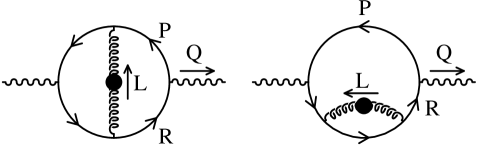
Figure 1: The two-loop diagrams contributing to photon and dilepton production.

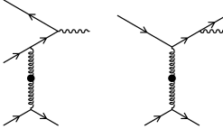
Figure 2: Important processes contained in the above 2-loop diagrams.

These processes are in fact enhanced by a strong sensitivity to the forward emission of the photon, due to a collinear singularity regularized by a thermal mass of order $gT$ where $g$ is the gauge coupling. In particular, the process on the left of figure 2 has been found to enhance considerably the rate of hard photons [27]. This collinear enhancement mechanism has also been shown to play a role in multi-loop diagrams belonging to the class of ladder corrections and self-energy-corrections [29, 30, 31, 8, 32, 33], and a resummation of this family of diagrams has been carried out in [32, 33]. The effect of this resummation, also known as Landau-Pomeranchuk-Migdal (LPM) effect [34, 35, 36], leads to a small reduction (by about 25% for photons in the range interesting for phenomenology) of the photon rate.

However, the strength of the LPM suppression decreases as one increases the invariant mass of the photon since the photon mass helps to regularize the collinear singularities. It is therefore expected that the dilepton rate can be accounted for by limiting oneself to a 2-loop calculation, and that the production of hard dileptons of intermediate invariant mass is dominated by the process shown on the left of figure 2. Under this assumption, the calculation of [27] has been extended recently to the case where the photon mass cannot be neglected any longer, with emphasis on the “off-shell annihilation” process that was already dominant for hard photons [37]. In this paper, we found a simple generalization to the case of massive photons of the formula known for the imaginary part of the real photon polarization tensor. This formula reads:

$$\!\!\!\!{\rm Im}\,\Pi_{{}_{R}}{}_{\mu}^{\mu}(Q)\approx-{{e^{2}g^{2}N_{c}C_{{}_{F}}}\over{2\pi^{4}}}{T\over{q_{0}^{2}}}\int\limits_{-\infty}^{+\infty}dp_{0}[n_{{}_{F}}(r_{0})-n_{{}_{F}}(p_{0})]$$

$$\quad\times\left\{(p_{0}^{2}+r_{0}^{2})(J_{{}_{T}}-J_{{}_{L}})+2{{Q^{2}p_{0}r_{0}+M_{\infty}^{2}(p_{0}^{2}+r_{0}^{2})}\over{M_{\rm eff}^{2}}}(K_{{}_{T}}-K_{{}_{L}})\right\}\,.$$ (1)

with $r_{0}\equiv p_{0}+q_{0}$ and

$$\!\!\!\!\!J_{{}_{T,L}}\equiv M_{\rm eff}^{2}\int\limits_{0}^{1}\!{{dx}\over{x}}{\rm Im}\,\Pi_{{}_{T,L}}(x)\!\int\limits_{0}^{+\infty}\!\!dw{{\sqrt{w/(w+4)}{\rm tanh}^{-1}\sqrt{w/(w+4)}}\over{(M_{\rm eff}^{2}w+{\rm Re}\,\Pi_{{}_{T,L}}(x))^{2}+({\rm Im}\,\Pi_{{}_{T,L}}(x))^{2}}}\;,$$

$$\!\!\!\!\!K_{{}_{T,L}}\equiv M_{\rm eff}^{2}\int\limits_{0}^{1}\!{{dx}\over{x}}{\rm Im}\,\Pi_{{}_{T,L}}(x)\!\int\limits_{0}^{+\infty}\!\!{{dw}\over w}{{\sqrt{w/(w+4)}{\rm tanh}^{-1}\sqrt{w/(w+4)}-w/4}\over{(M_{\rm eff}^{2}w+{\rm Re}\,\Pi_{{}_{T,L}}(x))^{2}+({\rm Im}\,\Pi_{{}_{T,L}}(x))^{2}}}\;,$$

where the $\Pi_{{}_{T,L}}$ are the transverse and longitudinal self-energies resummed on the gluon propagator, and where we denote

$$M_{\rm eff}^{2}\equiv M_{\infty}^{2}+{{Q^{2}}\over{q_{0}^{2}}}p_{0}r_{0}\;,$$ (3)

with $M_{\infty}$ the thermal mass of a hard quark ($M_{\infty}^{2}=g^{2}C_{{}_{F}}T^{2}/4$). The functions $\Pi_{{}_{T,L}}$ are the usual transverse and longitudinal HTL gluon self-energies:

$$\Pi_{{}_{T}}(L)=3m_{\rm g}^{2} \left[{{x^{2}}\over 2}+{{x(1-x^{2})}\over{4}}\ln\left({{x+1}\over{x-1}}\right)\right]$$

$$\Pi_{{}_{L}}(L)=3m_{\rm g}^{2} \left[(1-x^{2})-{{x(1-x^{2})}\over{2}}\ln\left({{x+1}\over{x-1}}\right)\right]\;,$$

where we denote $x\equiv l_{0}/l$ and where $m_{\rm g}^{2}\equiv g^{2}T^{2}[N_{c}+N_{{}_{F}}/2]/9$ is the gluon thermal mass in a $SU(N_{c})$ gauge theory with $N_{{}_{F}}$ flavors.

Therefore, in addition to the function $J_{{}_{T,L}}$ already introduced in the case of quasi-real photons, we need two new functions $K_{{}_{T,L}}$ for the term proportional to the photon invariant mass squared $Q^{2}$. All are dimensionless functions of the ratio of $M_{\rm eff}$ to the plasmon mass $m_{\rm g}$ which appears as a prefactor in the self-energies $\Pi_{{}_{T,L}}$. Up to now, the $J_{{}_{T,L}}$ and $K_{{}_{T,L}}$ have only been evaluated numerically ([26, 27], with a mistake corrected by [38, 39, 40]), which is sufficient for the case of real photons since in this case they are fixed numbers that depend only on the number of colors and flavors but not on kinematical parameters ($M_{\rm eff}^{2}=M_{\infty}^{2}$). However, the cost of this procedure increases significantly in the case of virtual photons since the value of $M_{\rm eff}^{2}$ depends on the invariant mass $Q$, energy $q_{0}$ and quark energy $p_{0}$. In addition, obtaining asymptotic limits is far from trivial at this point.

The aim of the present paper is to derive some analytical results regarding those functions. We first show how the integral over the variable $x$ can be performed exactly in the functions $J_{{}_{T,L}}$ and $K_{{}_{T,L}}$ by means of a simple sum-rule (section 2). This leads to either a very simple integral representation of these functions or even to closed formulas in terms of dilogarithms (section 3). Thanks to these results, we can easily study the asymptotic properties of the functions $J_{{}_{T,L}}$ and $K_{{}_{T,L}}$. Non trivial asymptotic expansions are obtained, which would have been very difficult to obtain otherwise (section 4). In section 5, we show that the above analytic results can also give some insight on the fact that the processes of figure 2 depend only on parameters like the gluon screening masses and the hard quark thermal mass, in a generic model where the quark gluon plasma is described as a gas of quasi-particles. Finally, we show that one can also calculate analytically the collision integral that appears in the resummation of ladder diagrams [32, 33] (section 6). In appendix A, we derive the asymptotic behavior of a function introduced at an intermediate stage. In appendix B, we prove analytically an anecdotical property which was first noticed numerically [41]: the integrals $J_{{}_{T}}$ and $J_{{}_{L}}$ are exactly opposite if $M_{\infty}=m_{\rm g}$ and $Q^{2}=0$.

2 Derivation of the sum-rule

We want to calculate the integral:

$$f(z)\equiv\int_{0}^{1}{{dx}\over{x}}{{2{\rm Im}\,\Pi(x)}\over{(z+{\rm Re}\,\Pi(x))^{2}+({\rm Im}\,\Pi(x))^{2}}}\;,$$ (5)

for a positive $z$, where $\Pi(x)$ is some self-energy depending only on $x\equiv k_{0}/k$ as is the case for instance with the HTL gluonic self-energy. The factor $1/x$ comes from a Bose-Einstein factor in the soft approximation $dk_{0}n_{{}_{B}}(k_{0})\approx Tdk_{0}/k_{0}=Tdx/x$. The first step in this calculation is to rewrite it as

$$f(z)=\int_{0}^{1}{{dx}\over{x}}(1-x^{2}){{2{\rm Im}\,\overline{\Pi}(x)}\over{(z(x^{2}-1)-{\rm Re}\,\overline{\Pi}(x))^{2}+({\rm Im}\,\overline{\Pi}(x))^{2}}}\;,$$ (6)

where we define $\overline{\Pi}(x)\equiv(1-x^{2})\Pi(x)$. Interpreting now $z$ ($z>0$) as the square of a three-momentum $k$ and $x$ as the ratio $x=k_{0}/k$, we have

$${{-2{\rm Im}\,\overline{\Pi}(x)}\over{(z(x^{2}-1)-{\rm Re}\,\overline{\Pi}(x))^{2}+({\rm Im}\,\overline{\Pi}(x))^{2}}} =2{\rm Re}\,{i\over{k_{0}^{2}-k^{2}-\overline{\Pi}(k_{0},k)+ik_{0}\epsilon}}$$ (7)

$$\equiv\overline{\rho}(k_{0},k)\;.$$

Note that this function is nothing but the spectral function $\overline{\rho}(k_{0},k)$ associated with the “propagator” appearing in the right hand side. This is what enables us to relate the integral

$$f(z)=-\int\limits_{0}^{1}{{dx}\over x}(1-x^{2})\overline{\rho}(\sqrt{z}x,\sqrt{z})$$ (8)

to the spectral representation of this propagator. Indeed, it is known that the resummed propagator $i/(K^{2}-\overline{\Pi}(K))$ is related to its spectral function $\overline{\rho}(k_{0},k)$ via the following spectral representation [42, 43]:

$${i\over{k_{0}^{2}-k^{2}-\overline{\Pi}(k_{0}/k)+ik_{0}\epsilon}}=\int_{0}^{+\infty}{{dE}\over{\pi}}E\overline{\rho}(E,k){{i}\over{k_{0}^{2}-E^{2}+ik_{0}\epsilon}}\;.$$ (9)

Taking the real part of this identity, one recovers the definition Eq. (7) of the spectral function. Taking its imaginary part and denoting $E\equiv kx$ and $k_{0}=ky$, one obtains the following non-trivial integral:

$$\ \int_{0}^{+\infty}{{dx}\over{\pi}}x\overline{\rho}(kx,k){1\over{y^{2}-x^{2}}}={{k^{2}(y^{2}-1)-{\rm Re}\,\overline{\Pi}(y)}\over{(k^{2}(y^{2}-1)-{\rm Re}\,\overline{\Pi}(y))^{2}+({\rm Im}\,\overline{\Pi}(y))^{2}}}\;.$$ (10)

Taking the limit $y\to\infty$, we find

$$\int_{0}^{+\infty}{{dx}\over{\pi}}x\overline{\rho}(kx,k)={1\over{k^{2}-\lim_{y\to\infty}{\rm Re}\,\overline{\Pi}(y)/y^{2}}}={1\over{k^{2}+{\rm Re}\,\Pi(\infty)}}\;.$$ (11)

Having in mind that $\Pi(y)$ is a gluonic self-energy obtained from the hard thermal loop approximation, its imaginary part vanishes if $y\geq 1$ and therefore does not contribute in the limit $y\to\infty$. Alternatively, taking the limit $y\to 0$ and assuming similarly that ${\rm Im}\,\Pi(y=0)=0$, we obtain:

$$\int_{0}^{+\infty}{{dx}\over{\pi}}{1\over x}\overline{\rho}(kx,k)={1\over{k^{2}+{\rm Re}\,\Pi(0)}}\;.$$ (12)

We can combine these two relations into

$$\int_{0}^{+\infty}{{dx}\over{x}}(1-x^{2})\overline{\rho}(kx,k)=\pi\left[{1\over{k^{2}+{\rm Re}\,\Pi(0)}}-{1\over{k^{2}+{\rm Re}\,\Pi(\infty)}}\right]\;.$$ (13)

In order to obtain from there the function $f(z)$, we need to subtract the contribution coming from $x$ between $1$ and $+\infty$. Fortunately, since ${\rm Im}\,\Pi(x)=0$ for $x\geq 1$, the contribution in this range comes only from the poles of the propagator $i/(K^{2}-\overline{\Pi}(K))$, via the formula

$$\int_{1}^{+\infty}{{dx}\over x}(1-x^{2})\overline{\rho}(kx,k)=\pi\sum_{{\rm poles\ }x_{i}}{{Z(x_{i})}\over{k^{2}}}{{1-x_{i}^{2}}\over{x_{i}^{2}}}\;,$$ (14)

where $Z(x_{i})$ is the residue of the propagator at the corresponding pole. For the above propagator, the equation that determines the poles is

$$k^{2}(x^{2}-1)={\rm Re}\,\overline{\Pi}(x)=(1-x^{2}){\rm Re}\,\Pi(x)\;.$$ (15)

This “dispersion equation” has a trivial solution $x=1$, which does not contribute when plugged in Eq. (14) because the other factors in the integrand vanish if $x=1$. Any non trivial pole would be a solution of the equation

$$k^{2}+{\rm Re}\,\Pi(x)=0\;,$$ (16)

but under the reasonable assumption that the resummation of the self-energy $\Pi(x)$ leads to well behaved quasi-particles (i.e. that the equation $k_{0}^{2}-k^{2}=\Pi(k_{0}/k)$ has a solution for every value of $k_{0}/k$ larger than $1$), we have ${\rm Re}\,\Pi(x)\geq 0$ for $x>1$ and therefore there are no additional poles. As a consequence, the integral of Eq. (13) does not receive any contribution from the range $x\in[1,+\infty]$, and we can write directly a closed expression for the function $f(z)$:

$$f(z)=\!\int_{0}^{1}\!{{dx}\over{x}}{{2{\rm Im}\,\Pi(x)}\over{(z+{\rm Re}\,\Pi(x))^{2}+({\rm Im}\,\Pi(x))^{2}}}=\pi\left[{1\over{z+{\rm Re}\,\Pi(\infty)}}\!-\!{1\over{z+{\rm Re}\,\Pi(0)}}\right]\,.$$ (17)

This is the basic sum-rule from which we are going to derive some results regarding photon production by a quark-gluon plasma. The validity of this result can also be checked numerically.

It may be useful to recall that, even if the derivation has been made having in mind a hard thermal loop for the self-energy $\Pi$, this result has a broader range of validity. In fact, it is valid for any self-energy satisfying the following assumptions:

1. $\Pi$ depends only on $x\equiv k_{0}/k$

2. ${\rm Im}\,\Pi(x=0)=0$

3. ${\rm Im}\,\Pi(x)=0$ if $x\geq 1$

4. ${\rm Re}\,\Pi(x)\geq 0$ if $x\geq 1$.

Note that the condition (1) can in fact be relaxed since what is done here can be reproduced if the self-energy depends separately on $k$ and $x$, the only difference being that the result would depend on $k$. The condition (2) is always true. Conditions (3) and (4) depend on the nature of the resummation under consideration, but are reasonable approximations in any system of well defined quasiparticles.

In [26], a formula for the photon rate based on sum rules was also presented. However, in this paper, the use of sum rules led only to a very complicated result (involving explicitly the gluon dispersion equations as well as the residues of the gluon poles) that was not useful for any practical purpose. By comparing the two methods, we can trace the simplification achieved in the present paper to a different choice for the integration variables. Indeed, in [26] the sum rules were applied to an integral over the variables $x\equiv l_{0}/l$, $l=|{\tenimbf l}|$ (where $L$ is the momentum of the exchanged gluon), while in the present approach, we take as independent integration variables $x$ and $w\equiv-L^{2}/M_{\rm eff}^{2}=l^{2}(1-x^{2})/M_{\rm eff}^{2}$. It appears that trading $l$ in favor of $w$ before using sum rules to perform the integral over $x$ leads to a dramatic simplification of the result, because some non trivial parts of the $x$ dependence get absorbed in the new variable $w$. There are in fact many sum rules satisfied by the HTL spectral functions. The interested reader may find other examples in [44, 45, 46].

3 Expression of $J_{{}_{T,L}}$ and $K_{{}_{T,L}}$

Thanks to the formula derived in the previous section, one can first simplify the functions $J_{{}_{T,L}}$ and $K_{{}_{T,L}}$ so that we have only one-dimensional integrals over the variable $w$:

$$J_{{}_{T,L}}={\pi\over 2}\int\limits_{0}^{+\infty}dw\sqrt{w\over{w+4}}{\rm tanh}^{-1}\sqrt{w\over{w+4}}$$

$$\qquad\qquad\qquad\times\left[{1\over{w+{{{\rm Re}\,\Pi_{{}_{T,L}}(\infty)}\over{M_{\rm eff}^{2}}}}}-{1\over{w+{{{\rm Re}\,\Pi_{{}_{T,L}}(0)}\over{M_{\rm eff}^{2}}}}}\right]\;,$$

$$K_{{}_{T,L}}={\pi\over 2}\int\limits_{0}^{+\infty}{{dw}\over{w}}\left[\sqrt{w\over{w+4}}{\rm tanh}^{-1}\sqrt{w\over{w+4}}-{w\over 4}\right]$$

$$\qquad\qquad\qquad\times\left[{1\over{w+{{{\rm Re}\,\Pi_{{}_{T,L}}(\infty)}\over{M_{\rm eff}^{2}}}}}-{1\over{w+{{{\rm Re}\,\Pi_{{}_{T,L}}(0)}\over{M_{\rm eff}^{2}}}}}\right]\;.$$ (18)

At this point, using the change of variable $u\equiv\sqrt{w/(w+4)}$, we can write in a simpler way the following elementary integrals:

$$\int\limits_{0}^{+\infty}dw\sqrt{w\over{w+4}}{\rm tanh}^{-1}\sqrt{w\over{w+4}}\left[{1\over{w}}-{1\over{w+a}}\right]=2F\Big{(}{4\over a}\Big{)}\;,$$

$$\int\limits_{0}^{+\infty}{{dw}\over{w}}\left[\sqrt{w\over{w+4}}{\rm tanh}^{-1}\sqrt{w\over{w+4}}-{w\over 4}\right]\left[{1\over{w}}-{1\over{w+a}}\right]$$

$$\qquad\qquad\qquad\qquad={1\over 4}\ln\Big{(}{1\over a}\Big{)}+{1\over 2}-{2\over a}F\Big{(}{4\over a}\Big{)}\;,$$ (19)

where we define the function

$$F(x)\equiv\int\limits_{0}^{1}du{{{\rm tanh}^{-1}(u)}\over{(x-1)u^{2}+1}}\;.$$ (20)

Recalling now the following properties of the HTL self-energy of the gluon [14]

$${\rm Re}\,\Pi_{{}_{T,L}}(\infty)=m_{\rm g}^{2}$$

$${\rm Re}\,\Pi_{{}_{T}}(0)=0$$

$${\rm Re}\,\Pi_{{}_{L}}(0)=3m_{\rm g}^{2}$$ (21)

where $m_{\rm g}$ is the plasmon mass, we easily obtain the following expressions in terms of the function $F(x)$:

$$J_{{}_{T}}=-\pi F\Big{(}{{4M_{\rm eff}^{2}}\over{m_{\rm g}^{2}}}\Big{)}\;,$$

$$J_{{}_{L}}=\pi\left[F\Big{(}{{4M_{\rm eff}^{2}}\over{3m_{\rm g}^{2}}}\Big{)}-F\Big{(}{{4M_{\rm eff}^{2}}\over{m_{\rm g}^{2}}}\Big{)}\right]\;,$$

$$K_{{}_{T}}=\pi\left[{{M_{\rm eff}^{2}}\over{m_{\rm g}^{2}}}F\Big{(}{{4M_{\rm eff}^{2}}\over{m_{\rm g}^{2}}}\Big{)}-{1\over 4}-{1\over 8}\ln\Big{(}{{M_{\rm eff}^{2}}\over{m_{\rm g}^{2}}}\Big{)}\right]\;,$$

$$K_{{}_{L}}=\pi\left[-{1\over 8}\ln(3)+{{M_{\rm eff}^{2}}\over{m_{\rm g}^{2}}}\left(F\Big{(}{{4M_{\rm eff}^{2}}\over{m_{\rm g}^{2}}}\Big{)}-{1\over 3}F\Big{(}{{4M_{\rm eff}^{2}}\over{3m_{\rm g}^{2}}}\Big{)}\right)\right]\;.$$ (22)

Therefore, those results demonstrate that in order to study the properties of the functions $J_{{}_{T,L}}$ and $K_{{}_{T,L}}$, one needs only to study the properties of the much simpler function $F(x)$. In fact, it is even possible to write the function $F(x)$ in closed form in terms of dilogarithms. We are not going to make use of this possibility here since it is simpler to keep $F(x)$ in its integral form given by Eq. (20).

One must stress the fact that all these functions depend only on the ratio of two masses. In the case of real photons ($Q^{2}=0$), we have in addition $M_{\rm eff}^{2}=M_{\infty}^{2}$ and for $N_{c}=3$ colors, we can write:

$${{4M_{\infty}^{2}}\over{3m_{\rm g}^{2}}}={8\over{6+N_{{}_{F}}}}\;,$$ (24)

i.e. the temperature and strong coupling constant also drop out of this ratio. It appears that there is an additional (and purely accidental) simplification for $N_{{}_{F}}=2$ flavors: in this case, the differences $J_{{}_{L}}-J_{{}_{T}}$ and $K_{{}_{L}}-K_{{}_{T}}$ can be expressed in a very simple fashion:

$$J_{{}_{L}}-J_{{}_{T}}\Big{|}_{N_{c}=3,N_{{}_{F}}=2}=\pi\ln(2)\;,$$

$$K_{{}_{L}}-K_{{}_{T}}\Big{|}_{N_{c}=3,N_{{}_{F}}=2}={\pi\over 4}(1-2\ln(2))\;.$$ (25)

For the case of $N_{{}_{F}}=3$ flavors, the results are less simple, but one can still obtain explicit expressions:

$$J_{{}_{L}}-J_{{}_{T}}\Big{|}_{N_{c}=3,N_{{}_{F}}=3}=\pi\Big{[}{{\pi^{2}}\over{8}}-{{33}\over 8}\ln^{2}(2)+3\ln(2)\ln(3)$$

$$\qquad\qquad\qquad\qquad\qquad\quad-{3\over 2}{\rm Li}_{2}\Big{(}{3\over 4}\Big{)}-{3\over 2}{\rm Li}_{2}\Big{(}-{1\over 2}\Big{)}\Big{]}\;,$$

$$K_{{}_{L}}-K_{{}_{T}}\Big{|}_{N_{c}=3,N_{{}_{F}}=3}=\pi\Big{[}{1\over 4}-{{\pi^{2}}\over{36}}+{{\ln(2)}\over 8}-{{\ln(3)}\over 4}+{{11}\over{12}}\ln^{2}(2)$$

$$\qquad\qquad\qquad\qquad\qquad\quad-{2\over 3}\ln(2)\ln(3)+{1\over 3}{\rm Li}_{2}\Big{(}{3\over 4}\Big{)}+{1\over 3}{\rm Li}_{2}\Big{(}-{1\over 2}\Big{)}\Big{]}\;.$$

Had these exact formulas been known, the confusion due to the erroneous factor $4$ in the numerical evaluation of these coefficients in [27] would have been avoided [40].

4 Asymptotic behavior of $J_{{}_{T,L}}$ and $K_{{}_{T,L}}$

4.1 Limit $M_{\rm eff}\ll m_{\rm g}$

Using the above results, we can recover in a rather simple and elegant way all the asymptotic limits given in [26] for $J_{{}_{T,L}}$, as well as the limits used for $K_{{}_{T,L}}$ in order to obtain the behavior of 2-loop dilepton production near the threshold $Q^{2}=4M_{\infty}^{2}$ (a region which is dominated by small values of $M_{\rm eff}^{2})$ [37].

To that effect, we need only the behavior of $F(x)$ when $x\to 0$. This is derived in the appendix A, where we prove that:

$$F(x)\mathrel{\mathop{\kern 0.0pt=}\limits_{x\to 0^{+}}}{1\over 8}\ln^{2}\Big{(}{4\over x}\Big{)}+{{\pi^{2}}\over{24}}+{\cal O}\Big{(}x\ln^{2}(1/x)\Big{)}\;.$$ (27)

Thanks to this formula, a trivial calculation gives

$$J_{{}_{T}}\mathrel{\mathop{\kern 0.0pt\approx}\limits_{M_{\rm eff}\ll m_{\rm g}}}-{\pi\over 8}\ln^{2}\Big{(}{{m_{\rm g}^{2}}\over{M_{\rm eff}^{2}}}\Big{)}\;,$$

$$J_{{}_{L}}\mathrel{\mathop{\kern 0.0pt\approx}\limits_{M_{\rm eff}\ll m_{\rm g}}}{{\pi\ln(3)}\over 4}\ln\Big{(}{{m_{\rm g}^{2}}\over{M_{\rm eff}^{2}}}\Big{)}\;,$$

$$K_{{}_{T}}\mathrel{\mathop{\kern 0.0pt\approx}\limits_{M_{\rm eff}\ll m_{\rm g}}}{\pi\over 8}\left[\ln\Big{(}{{m_{\rm g}^{2}}\over{M_{\rm eff}^{2}}}\Big{)}-2\right]\;,$$

$$K_{{}_{L}}\mathrel{\mathop{\kern 0.0pt\approx}\limits_{M_{\rm eff}\ll m_{\rm g}}}-{{\pi\ln(3)}\over 8}\;.$$ (28)

These relations in fact go well beyond the results for $J_{{}_{T,L}}$ obtained in [26], since in this new approach we obtain for free the prefactor of the leading term and we could even have calculated some subleading terms, down to the constant term.

4.2 Limit $M_{\rm eff}\gg m_{\rm g}$

Using Eqs. (22), it is also very simple to obtain the behavior of the functions $J_{{}_{T,L}}$ and $K_{{}_{T,L}}$ in the opposite limit where $M_{\rm eff}\gg m_{\rm g}$. In order to do that, we need to know the behavior of $F(x)$ for large values of $x$. The following formula is also derived in appendix A:

$$F(x)\mathrel{\mathop{\kern 0.0pt=}\limits_{x\gg 1}}{{\ln(x)}\over{2x}}+{{1-\ln(2)}\over{x}}+{{\ln(x)}\over{3x^{2}}}+{{5-6\ln(2)}\over{9x^{2}}}+{\cal O}\Big{(}{{\ln(x)}\over{x^{3}}}\Big{)}\;.$$ (29)

From this formula, it is easy to obtain

$$J_{{}_{T}}\mathrel{\mathop{\kern 0.0pt\approx}\limits_{M_{\rm eff}\gg m_{\rm g}}}-{\pi\over 8}{{m_{\rm g}^{2}}\over{M_{\rm eff}^{2}}}\ln\Big{(}{{M_{\rm eff}^{2}}\over{m_{\rm g}^{2}}}\Big{)}\;,$$

$$J_{{}_{L}}\mathrel{\mathop{\kern 0.0pt\approx}\limits_{M_{\rm eff}\gg m_{\rm g}}}{\pi\over 4}{{m_{\rm g}^{2}}\over{M_{\rm eff}^{2}}}\ln\Big{(}{{M_{\rm eff}^{2}}\over{m_{\rm g}^{2}}}\Big{)}\approx-2J_{{}_{T}}\;,$$

$$K_{{}_{T}}\mathrel{\mathop{\kern 0.0pt\approx}\limits_{M_{\rm eff}\gg m_{\rm g}}}{\pi\over{48}}{{m_{\rm g}^{2}}\over{M_{\rm eff}^{2}}}\ln\Big{(}{{M_{\rm eff}^{2}}\over{m_{\rm g}^{2}}}\Big{)}\;,$$

$$K_{{}_{L}}\mathrel{\mathop{\kern 0.0pt\approx}\limits_{M_{\rm eff}\gg m_{\rm g}}}-{\pi\over{24}}{{m_{\rm g}^{2}}\over{M_{\rm eff}^{2}}}\ln\Big{(}{{M_{\rm eff}^{2}}\over{m_{\rm g}^{2}}}\Big{)}\approx-2K_{{}_{T}}\;.$$ (30)

5 Beyond the HTL approximation

In section 2, we mentioned the fact that the sum rule in Eq. (17) is in fact valid for a gluon self-energy $\Pi$ more general than the standard case of hard thermal loops. Assuming it can be applied, we see that the result depends only on the four numbers ${\rm Re}\,\Pi_{{}_{T,L}}(\infty)$ and ${\rm Re}\,\Pi_{{}_{T,L}}(0)$. The first two are the plasmon mass (longitudinal) and the mass of the transverse gluon at zero momentum, and can be shown to be equal thanks to Slavnor-Taylor identities [47, 48, 49]. Physically, this property means that there is no way to distinguish transverse and longitudinal modes for a particle at rest. Therefore, we need only to introduce one plasmon mass:

$${\rm Re}\,\Pi_{{}_{T}}(\infty)={\rm Re}\,\Pi_{{}_{L}}(\infty)\equiv m_{P}^{2}\;.$$ (31)

The quantities on the second line are squares of the screening masses for the transverse and longitudinal static gluon exchanges. The longitudinal screening mass is the familiar Debye mass:

$$m_{D}^{2}\equiv{\rm Re}\,\Pi_{{}_{L}}(0)$$ (32)

In the HTL approximation, there is no screening for the transverse static gluons, but this is not expected to hold generally. The corresponding screening mass is the magnetic mass, and is denoted

$$m_{\rm mag}^{2}\equiv{\rm Re}\,\Pi_{{}_{T}}(0)\;.$$ (33)

In terms of those parameters, it is straightforward to write down the expressions of $J_{{}_{T,L}}$ and $K_{{}_{T,L}}$ for photon production in a description where we use gluon propagators that are more general than the HTL propagators:

$$J_{{}_{T}}=\pi\left[F\Big{(}{{4M_{\rm eff}^{2}}\over{m_{\rm mag}^{2}}}\Big{)}-F\Big{(}{{4M_{\rm eff}^{2}}\over{m_{P}^{2}}}\Big{)}\right]\;,$$

$$J_{{}_{L}}=\pi\left[F\Big{(}{{4M_{\rm eff}^{2}}\over{m_{D}^{2}}}\Big{)}-F\Big{(}{{4M_{\rm eff}^{2}}\over{m_{P}^{2}}}\Big{)}\right]\;,$$

$$K_{{}_{T}}=\pi\left[-{1\over 8}\ln\Big{(}{{m_{\rm mag}^{2}}\over{m_{P}^{2}}}\Big{)}+{{M_{\rm eff}^{2}}\over{m_{P}^{2}}}F\Big{(}{{4M_{\rm eff}^{2}}\over{m_{P}^{2}}}\Big{)}-{{M_{\rm eff}^{2}}\over{m_{\rm mag}^{2}}}F\Big{(}{{4M_{\rm eff}^{2}}\over{m_{\rm mag}^{2}}}\Big{)}\right]\;,$$

$$K_{{}_{L}}=\pi\left[-{1\over 8}\ln\Big{(}{{m_{D}^{2}}\over{m_{P}^{2}}}\Big{)}+{{M_{\rm eff}^{2}}\over{m_{P}^{2}}}F\Big{(}{{4M_{\rm eff}^{2}}\over{m_{P}^{2}}}\Big{)}-{{M_{\rm eff}^{2}}\over{m_{D}^{2}}}F\Big{(}{{4M_{\rm eff}^{2}}\over{m_{D}^{2}}}\Big{)}\right]\;.$$ (34)

It is easy to check that these relations fall back to Eqs. (22) if we set $m_{\rm mag}=0$, $m_{P}=m_{\rm g}$ and $m_{D}=\sqrt{3}m_{\rm g}$, which are the relations between masses in the HTL framework.

There is another general property of the processes of figure 2 which is worth mentioning here. Their rate in fact depends only on the combinations $J_{{}_{T}}-J_{{}_{L}}$ and $K_{{}_{T}}-K_{{}_{L}}$ (see Eq. (1)) after one has summed the contributions of transverse and longitudinal gluons. Using the above formulas, we obtain:

$$J_{{}_{T}}-J_{{}_{L}}=\pi\left[F\Big{(}{{4M_{\rm eff}^{2}}\over{m_{\rm mag}^{2}}}\Big{)}-F\Big{(}{{4M_{\rm eff}^{2}}\over{m_{D}^{2}}}\Big{)}\right]\;,$$

$$K_{{}_{T}}-K_{{}_{L}}=\pi\left[{1\over 8}\ln\Big{(}{{m_{D}^{2}}\over{m_{\rm mag}^{2}}}\Big{)}+{{M_{\rm eff}^{2}}\over{m_{D}^{2}}}F\Big{(}{{4M_{\rm eff}^{2}}\over{m_{D}^{2}}}\Big{)}-{{M_{\rm eff}^{2}}\over{m_{\rm mag}^{2}}}F\Big{(}{{4M_{\rm eff}^{2}}\over{m_{\rm mag}^{2}}}\Big{)}\right]\;.$$ (35)

In other words, all the dependence on the plasmon mass drops out for the processes of figure 2. This property is in fact reasonable since we are looking at processes that involve only space-like gluons, and it would have been surprising if the result had depended on the plasmon mass, a property of time-like gluons. The practical consequence of this for a phenomenological approach to photon production based on some quasi-particle picture is that we do not need to know the full gluon propagator, but only the two screening masses and the quark thermal mass. Note also that these quantities remain finite even if the magnetic mass is very small or vanishing.

In particular, it is now known from lattice calculations [50, 51] that the masses of quasi-particles increase when the temperature approaches the critical temperature from above, while at the same time the screening masses decrease. The formulas of this section are important to deal with such a situation, since they do not assume any particular relationship between the screening masses and the quasi-particle masses. For instance, for a temperature just above $T_{c}$, we can make use of Eqs. (30), and predict a suppression of the production rate of photons and low-mass dileptons simply due to the fact that screening masses are much smaller than the quasi-particle masses (in addition to the standard suppression due to the fact that the temperature is smaller).

6 Resummation of ladder diagrams and LPM effect

6.1 Integral equation in momentum space

The authors of [32, 33] performed the resummation of all the ladder diagrams, as well as all the self-energy corrections that are required to preserve gauge invariance, in order to account for the LPM effect in the production of real photons. Indeed, such photons may have a formation time larger than the mean free path of the quarks in the medium [31], so that multiple quark scatterings contribute coherently to the formation of the photon.

In the formulation of [32, 33], the imaginary part of the retarded photon polarization tensor is given by

$$\!\!\!\!{\rm Im}\,\Pi_{{}_{R}}{}_{\mu}^{\mu}(Q)\approx{{e^{2}N_{c}}\over{8\pi}}\int_{-\infty}^{+\infty}dp_{0}\,\;[n_{{}_{F}}(r_{0})-n_{{}_{F}}(p_{0})]\;{{p_{0}^{2}+r_{0}^{2}}\over{p_{0}^{2}r_{0}^{2}}}$$

$$\qquad\qquad\qquad\times{\rm Re}\,\int{{d^{2}{\tenimbf p}_{\perp}}\over{(2\pi)^{2}}}\;{\tenimbf p}_{\perp}\cdot{\tenimbf f}({\tenimbf p}_{\perp})\;,$$

(36)

where $r_{0}\equiv p_{0}+q_{0}$ and ${\tenimbf f}({\tenimbf p}_{\perp})$ is a dimensionless transverse vector that represents the resummed coupling of a quark to the transverse modes of the photon, satisfying the following integral equation

$$2{\tenimbf p}_{\perp}=i\delta E{\tenimbf f}({\tenimbf p}_{\perp})+g^{2}C_{{}_{F}}T\int{{d^{2}{\tenimbf l}_{\perp}}\over{(2\pi)^{2}}}{\cal C}({\tenimbf l}_{\perp})[{\tenimbf f}({\tenimbf p}_{\perp})-{\tenimbf f}({\tenimbf p}_{\perp}+{\tenimbf l}_{\perp})]\;,$$ (37)

where $\delta E\equiv q_{0}({\tenimbf p}_{\perp}^{2}+M_{\rm eff}^{2})/(2p_{0}r_{0})$ and in which ${\cal C}({\tenimbf l}_{\perp})$ is the collision integral defined by

$${\cal C}({\tenimbf l}_{\perp})\equiv\int{{dl_{0}dl_{z}}\over{(2\pi)^{2}}}2\pi\delta(l_{0}-l_{z})\,{1\over{l_{0}}}$$

$$\qquad\quad\times\sum_{\alpha=L,T}{{2{\rm Im}\,\Pi_{\alpha}(L)}\over{(L^{2}-{\rm Re}\,\Pi_{\alpha}(L))^{2}+({\rm Im}\,\Pi_{\alpha}(L))^{2}}}\;P_{\alpha}^{\mu\nu}(L)\widehat{Q}_{\mu}\widehat{Q}_{\nu}\;,$$ (38)

with $\widehat{Q}_{\mu}\equiv(1,{\tenimbf q}/q)$ and $P_{{}_{T,L}}^{\mu\nu}(L)$ the transverse or longitudinal projector for a gluon of momentum $L$. Note that $\delta E^{-1}$ is nothing but the typical formation time of the photon [31]. Note also that in an iterative solution of these integral equations, the first term that contributes to the imaginary part of the photon polarization tensor is of order $g^{2}$ since ${\tenimbf f}({\tenimbf p}_{\perp})$ and $g({\tenimbf p}_{\perp})$ are purely imaginary at the order $g^{0}$. This reflects the fact that the direct production of a photon by the processes $q\bar{q}\to\gamma$ or $q\to q\gamma$ is kinematically forbidden. This remark ceases to be valid if $\delta E$ can vanish, in which case an $i\epsilon$ prescription must be used, so that the zeroth order solution can have a real part. This happens if $M_{\rm eff}^{2}$ can become negative, i.e. if $Q^{2}>4M_{\infty}^{2}$.

Using the fact that we have

$$P_{{}_{T}}^{\mu\nu}(L)\widehat{Q}_{\mu}\widehat{Q}_{\nu}={{l_{z}^{2}}\over{l^{2}}}-1=-P_{{}_{L}}^{\mu\nu}(L)\widehat{Q}_{\mu}\widehat{Q}_{\nu}\;,$$ (41)

and introducing the variable $x\equiv l_{0}/l$, we can rewrite the collision integral in Eq. (38) as

$$\!\!\!\!{\cal C}({\tenimbf l}_{\perp})={2\over\pi}\int_{0}^{1}{{dx}\over{x}}\;\left[{{{\rm Im}\,\Pi_{{}_{L}}(x)}\over{(l_{\perp}^{2}+{\rm Re}\,\Pi_{{}_{L}}(x))^{2}+({\rm Im}\,\Pi_{{}_{L}}(x))^{2}}}\right.$$

$$\qquad\qquad\qquad\qquad\left.-{{{\rm Im}\,\Pi_{{}_{T}}(x)}\over{(l_{\perp}^{2}+{\rm Re}\,\Pi_{{}_{T}}(x))^{2}+({\rm Im}\,\Pi_{{}_{T}}(x))^{2}}}\right]\;.$$ (43)

At this point, the sum rule derived in section 2 gives directly the result of the integral over the variable $x$, so that the collision integral can be rewritten as:

$${\cal C}({\tenimbf l}_{\perp})={1\over{l_{\perp}^{2}}}-{1\over{l_{\perp}^{2}+3m_{\rm g}^{2}}}\;.$$ (44)

We observe again that summing over the contributions of transverse and longitudinal gluon exchanges cancels the terms involving the plasmon mass.

6.2 Solution in the Bethe-Heitler regime

As a check, one can solve this integral equation iteratively up to the order $g^{2}$. Indeed, the naive term of order $g^{0}$ is purely imaginary, and drops out of the imaginary part of the photon polarization tensor (see Eq. (36)). For the function ${\tenimbf f}({\tenimbf p}_{\perp})$, this expansion gives:

$$\!\!\!\!\!\!{\rm Re}\;\int{{d^{2}{\tenimbf p}_{\perp}}\over{(2\pi)^{2}}}\;{\tenimbf p}_{\perp}\cdot{\tenimbf f}({\tenimbf p}_{\perp})\mathrel{\mathop{\kern 0.0pt=}\limits_{{\cal O}(g^{2})}}8g^{2}C_{{}_{F}}T{{(p_{0}r_{0})^{2}}\over{q_{0}^{2}}}\int{{d^{2}{\tenimbf p}_{\perp}}\over{(2\pi)^{2}}}\;{{{\tenimbf p}_{\perp}}\over{{\tenimbf p}_{\perp}^{2}+M_{\rm eff}^{2}}}$$

$$\qquad\qquad\cdot\int{{d^{2}{\tenimbf l}_{\perp}}\over{(2\pi)^{2}}}{\cal C}({\tenimbf l}_{\perp})\left[{{{\tenimbf p}_{\perp}}\over{{\tenimbf p}_{\perp}^{2}+M_{\rm eff}^{2}}}-{{{\tenimbf p}_{\perp}+{\tenimbf l}_{\perp}}\over{({\tenimbf p}_{\perp}+{\tenimbf l}_{\perp})^{2}+M_{\rm eff}^{2}}}\right]\;.$$

At this stage, performing the angular integrations is elementary. Making use of the following identity:

$$\int\limits_{0}^{+\infty}d(p_{\perp}^{2})\left({1\over{p_{\perp}^{2}+M_{\rm eff}^{2}}}-{1\over{\sqrt{(p_{\perp}^{2}+l_{\perp}^{2}+M_{\rm eff}^{2})^{2}-4p_{\perp}^{2}l_{\perp}^{2}}}}\right)=0\;,$$ (46)

this can be rewritten as:

$${\rm Re}\;\int{{d^{2}{\tenimbf p}_{\perp}}\over{(2\pi)^{2}}}\;{\tenimbf p}_{\perp}\cdot{\tenimbf f}({\tenimbf p}_{\perp})\mathrel{\mathop{\kern 0.0pt=}\limits_{{\cal O}(g^{2})}}-{{2g^{2}C_{{}_{F}}T}\over{\pi^{3}}}{{(p_{0}r_{0})^{2}}\over{q_{0}^{2}}}[J_{{}_{T}}-J_{{}_{L}}+2K_{{}_{T}}-2K_{{}_{L}}]\;.$$ (47)

Finally, plugging Eqs. (47) into Eq. (36) gives

$$\!\!\!\!{\rm Im}\,\Pi_{{}_{R}}{}_{\mu}^{\mu}(Q)\mathrel{\mathop{\kern 0.0pt=}\limits_{{\cal O}(g^{2})}}-{{e^{2}g^{2}N_{c}C_{{}_{F}}}\over{2\pi^{4}}}{T\over{q_{0}^{2}}}\int\limits_{-\infty}^{+\infty}dp_{0}[n_{{}_{F}}(r_{0})-n_{{}_{F}}(p_{0})]$$

$$\qquad\times\,(p_{0}^{2}+r_{0}^{2})[J_{{}_{T}}-J_{{}_{L}}+2K_{{}_{T}}-2K_{{}_{L}}]\;,$$ (48)

which is equivalent to Eq. (1) for real photons ($Q^{2}=0$, $M_{\rm eff}^{2}=M_{\infty}^{2}$). This proves the agreement between the perturbative approach followed in [37] and the resummation of the LPM corrections, if one formally keeps only the ${\cal O}(g^{2})$ terms. The fact that some terms proportional to $Q^{2}$ in Eq. (1) are not recovered in this limit is due to the fact that the LPM resummation of [32, 33] is limited to the transverse modes of the produced photon, while massive photons also have a physical longitudinal mode.

6.3 Reformulation as a differential equation

Since the collision integral appearing under the integral over ${\tenimbf l}_{\perp}$ is now known in closed form, it is possible to transform this integral equation into an ordinary differential equation by going to impact parameter space. We can first define

$${\tenimbf f}({\tenimbf p}_{\perp})\equiv\int d^{2}{\tenimbf b}\,e^{-i{\tenimbf p}_{\perp}\cdot{\tenimbf b}}{\tenimbf g}({\tenimbf b})\;.$$ (49)

Note that the order zero (in $g^{2}$) solution of the integral equation is

$${\tenimbf g}_{0}({\tenimbf b})=-{2\over\pi}{{p_{0}r_{0}}\over{q_{0}}}\nabla_{b}K_{0}(M_{\rm eff}b)={2\over\pi}{{p_{0}r_{0}}\over{q_{0}}}M_{\rm eff}\widehat{\tenimbf b}K_{1}(M_{\rm eff}b)\;,$$ (50)

where the $K_{i}$’s are modified Bessel functions of the second kind. For the higher order terms ${\tenimbf g}_{1}({\tenimbf b})$, one obtains the following equation for ${\tenimbf g}_{1}$

$$i{{q_{0}}\over{2p_{0}r_{0}}}(M_{\rm eff}^{2}-\Delta_{\perp}){\tenimbf g}_{1}({\tenimbf b})+g^{2}C_{{}_{F}}TD(m_{\rm g}b)({\tenimbf g}_{0}({\tenimbf b})+{\tenimbf g}_{1}({\tenimbf b}))=0\;,$$ (51)

with

$$D(m_{\rm g}b)\equiv{1\over{2\pi}}\left[\gamma+\ln\left({{\sqrt{3}m_{\rm g}b}\over{2}}\right)+K_{0}(\sqrt{3}m_{\rm g}b)\right]\;.$$ (52)

In addition, we have also

$${\rm Re}\;{\tenimbf p}_{\perp}\cdot\int{{d^{2}{\tenimbf p}_{\perp}}\over{(2\pi)^{2}}}{\tenimbf f}({\tenimbf p}_{\perp})=\lim_{b\to 0^{+}}{\rm Im}\;\nabla_{\perp}\cdot{\tenimbf g}_{1}({\tenimbf b})\;.$$ (53)

This differential equation can be further simplified by defining the following dimensionless quantities:

$$t\equiv M_{\rm eff}^{2}b^{2}\;,$$

$$u(t)\equiv{{\pi q_{0}}\over{2p_{0}r_{0}}}{\tenimbf b}\cdot{\tenimbf g}({\tenimbf b})\;.$$ (54)

This transformation leads to

$$4tu_{1}^{\prime\prime}(t)-u_{1}(t)+ig^{2}C_{{}_{F}}{{p_{0}r_{0}}\over{q_{0}}}{T\over{M_{\rm eff}^{2}}}D\left({{m_{\rm g}}\over{M_{\rm eff}}}\sqrt{t}\right)(u_{0}(t)+u_{1}(t))=0\;,$$ (55)

where the prime denotes the differentiation with respect to $t$, and where

$$u_{0}(t)\equiv\sqrt{t}K_{1}(\sqrt{t})\;.$$ (56)

The differential equation Eq. (55) depends on two dimensionless quantities. One is the ratio $m_{\rm g}/M_{\rm eff}$ of two masses, while the prefactor $g^{2}C_{{}_{F}}Tp_{0}r_{0}/q_{0}M_{\rm eff}^{2}$ can be interpreted (up to logarithms) as the ratio of the photon formation time to the quark mean free path. It is therefore the average number of scatterings that can contribute coherently to the production of a photon. The relevant quantity for the photon production rate is then given by

$${\rm Re}\;{\tenimbf p}_{\perp}\cdot\int{{d^{2}{\tenimbf p}_{\perp}}\over{(2\pi)^{2}}}{\tenimbf f}({\tenimbf p}_{\perp})={{4p_{0}r_{0}}\over{\pi q_{0}}}M_{\rm eff}^{2}\;{\rm Im}\;u_{1}^{\prime}(0)\;.$$ (57)

This differential equation must be supplemented by boundary conditions in order to define uniquely the solution. First, we have

$$u(0)=0\;,$$ (58)

which can be seen from its definition. Subtracting $u_{0}(0)=1$, this implies

$$u_{1}(0)=-1\;.$$ (59)

Unfortunately, we do not know the value of $u_{1}^{\prime}(0)$ but instead we know the value of $u(\infty)$. Indeed, assuming that ${\tenimbf f}({\tenimbf p}_{\perp})$ is regular enough, its Fourier transform is exponentially suppressed at large $b$. Therefore, $u(\infty)=0$. Since we already have $u_{0}(\infty)=0$, this implies

$$u_{1}(\infty)=0\;.$$ (60)

Therefore, the problem can be summarized as follows: we are looking for the (presumably complex) value of $u_{1}^{\prime}(0)$ that takes us from $u_{1}(0)=-1$ to $u_{1}(\infty)=0$. The imaginary part of this derivative term is then the coefficient that enters in the photon polarization tensor. Note also that since the term $u_{1}^{\prime\prime}$ and $u_{1}$ come with opposite signs in the combination $4tu_{1}^{\prime\prime}-u_{1}$ in Eq. (55), generic solutions are unstable and diverge as $t\to+\infty$ (they are in fact linear combinations of a function that diverges exponentially and of a function that goes exponentially to zero). It is only for a very specific value of $u_{1}^{\prime}(0)$ that one can make the coefficient of the diverging term zero, and have a solution that satisfies $u_{1}(\infty)=0$. This heuristic argument thereby justifies the uniqueness of the number $u_{1}^{\prime}(0)$ solving the problem.

6.4 Numerical solution

6.4.1 General principle

This reformulation of Eqs. (36) and (37) leads to a rather straightforward algorithm for a numerical solution. Differential problems with two-point boundary conditions are usually solved by iterative “shooting” methods [53], where one tries to make a guess for the missing initial condition (here, $u_{1}^{\prime}(0)$) and then corrects this value based on the discrepancy between the resulting end-point and the expected one.

Things are in fact much simpler for an affine equation, since only two trials, plus the knowledge of a solution of the complete equation, are enough to find the value of $u_{1}^{\prime}(0)$. Indeed, for a differential equation like (55), solutions have generically the following form:

$$u_{1}(t)=w(t)+\alpha_{1}w_{1}(t)+\alpha_{2}w_{2}(t)\;,$$ (61)

where $w(t)$ is a particular solution of the full equation, and $w_{1,2}(t)$ are two independent solutions of the corresponding homogeneous equation (i.e. (55) in which one would set $u_{0}$ to zero). Generically, it is convenient to chose these functions such that:

$$w(0)=0\;,\qquad w^{\prime}(0)=0\;,$$

$$w_{1}(0)=1\;,\qquad w_{1}^{\prime}(0)=0\;,$$

$$w_{2}(0)=0\;,\qquad w_{2}^{\prime}(0)=1\;.$$ (62)

If these solutions are known (at least numerically), the condition $u_{1}(0)=-1$ implies

$$\alpha_{1}=-1\;.$$ (63)

Then, using $u_{1}(+\infty)=0$, the second coefficient $\alpha_{2}$ is given by

$$\alpha_{2}=\lim_{t\to+\infty}{{w_{1}(t)-w(t)}\over{w_{2}(t)}}\;;$$ (64)

and thanks to our choice of initial conditions for $w,w_{1}$ and $w_{2}$, the value of $u_{1}^{\prime}(0)$ that solves the problem is simply given by

$$u_{1}^{\prime}(0)=\alpha_{2}\;.$$ (65)

6.4.2 Realistic algorithm

This algorithm is however not directly applicable in the case of Eq. (55), because the point $t=0$ is a singular point of the equation, and cannot be used to set initial conditions. Therefore, we have to chose another point in order to set the initial conditions. Let us call this point $t_{0}>0$, and assume

$$w(t_{0})=0\;,\qquad w^{\prime}(t_{0})=0\;,$$

$$w_{1}(t_{0})=1\;,\qquad w_{1}^{\prime}(t_{0})=0\;,$$

$$w_{2}(t_{0})=0\;,\qquad w_{2}^{\prime}(t_{0})=1\;,$$ (66)

instead of Eqs. (62). From these initial conditions, one must evolve numerically the functions $w,w_{1}$ and $w_{2}$ both forward and backward. Having in mind what has been said at the end of section 6.3, the three functions are going to diverge when $t\to+\infty$ (unless one has been very unlucky when choosing the initial conditions). The condition $u_{1}(+\infty)=0$ then implies

$$0=1+\alpha_{1}r_{1}+\alpha_{2}r_{2}\;,$$ (67)

where $r_{i}\equiv\lim_{t\to+\infty}w_{i}(t)/w(t)$. This gives a first linear relation between the two coefficients $\alpha_{1}$ and $\alpha_{2}$. Then, from the condition $u_{1}(0)=-1$, one can obtain

$$\alpha_{1}=\lim_{t\to 0^{+}}-{{w_{2}(t)-r_{2}(1+w(t))}\over{r_{1}w_{2}(t)-r_{2}w_{1}(t)}}\;.$$ (68)

At this point, the two coefficients $\alpha_{1,2}$ are known, and it is easy to find

$$u_{1}^{\prime}(0)=\lim_{t\to 0^{+}}w^{\prime}(t)+\alpha_{1}w_{1}^{\prime}(t)+\alpha_{2}w_{2}^{\prime}(t)\;.$$ (69)

This last step does not require any additional calculation, since the derivatives of $w,w_{1,2}$ are known numerically at this point. In summary, this algorithm reduces the problem of solving the integral equation (37) and then calculating the integral over ${\tenimbf p}_{\perp}$ in Eq. (36) to the numerical solution of a differential equation with three different initial conditions. A numerical analysis of Eq. (36) based along these lines will be presented elsewhere [52].

7 Conclusions

In this paper, we have derived a simple sum rule that enables to perform analytically some of the integrals involved in the thermal 2-loop photon production rate. Several applications of this sum rule have been presented. This sum rule also plays a role in the calculation of the collision integral that appears in the resummation of the ladder diagrams involved in the calculation of the LPM effect.

Appendix A Asymptotic behavior of $F(x)$

A.1 Large $x$ behavior of $F(x)$

At large values of the argument $x$, the asymptotic value of the function $F(x)$ introduced in Eq. (20) is very easy to obtain:

$$F(x) = \epsilon\int_{0}^{1}du{{{\rm tanh}^{-1}(u)}\over{u^{2}+\epsilon}}\qquad{\rm with}\qquad\epsilon\equiv{1\over{x-1}}\ll 1$$ (71)

$$= \epsilon\int_{0}^{1}du{{{\rm tanh}^{-1}(u)-u}\over{u^{2}+\epsilon}}+\epsilon\int_{0}^{1}du{u\over{u^{2}+\epsilon}}$$

$$= \epsilon\left[1-\ln(2)+{\cal O}(\epsilon\ln(1/\epsilon))\right]+\epsilon\ln\Big{(}{{1+\epsilon}\over\epsilon}\Big{)}\;,$$

i.e.

$$F(x)\mathrel{\mathop{\kern 0.0pt=}\limits_{x\to+\infty}}{{\ln(x)}\over{2x}}+{{1-\ln(2)}\over x}+{\cal O}\Big{(}{{\ln(x)}\over{x^{2}}}\Big{)}\;.$$ (72)

Let us add that if the variable $x$ goes to $-\infty$, one can obtain the correct asymptotic behavior by replacing $x$ by $-x$ in the previous expression (in particular $\ln(x)$ by $\ln|x|-i\pi$) while dropping the imaginary part, so that the previous asymptotic formula simply becomes:

$$F(x)\mathrel{\mathop{\kern 0.0pt=}\limits_{x\to-\infty}}{{\ln|x|}\over{2x}}+{{1-\ln(2)}\over x}+{\cal O}\Big{(}{{\ln|x|}\over{x^{2}}}\Big{)}\;.$$ (73)

A.2 Small $x$ behavior of $F(x)$

At small values of $x$, determining the expansion of $F(x)$ requires a little more work. Denoting $y\equiv 1/\sqrt{1-x}\approx 1+x/2$, we have

$$F(x) = {{y^{2}}\over 2}\int_{0}^{1}du\ln\Big{(}{{1+u}\over{1-u}}\Big{)}{1\over{y^{2}-u^{2}}}$$ (74)

$$= {y\over 4}\int_{0}^{1}du\ln\Big{(}{{1+u}\over{1-u}}\Big{)}\left[{1\over{y+u}}+{1\over{y-u}}\right]\;.$$

Let us notice first that the term in $1/(y+u)$ is finite in the limit $y\to 1$. Therefore, since we do not want to go beyond the constant terms, we can simply replace $y$ by $1$ in this term and get

$${1\over 4}\int\limits_{0}^{1}du\ln\Big{(}{{1+u}\over{1-u}}\Big{)}{1\over{1+u}}=-{1\over 4}\int\limits_{0}^{1}dv{{\ln(v)}\over{1+v}}={{\pi^{2}}\over{48}}\;.$$ (75)

The other term can be separated in two parts, the first one being

$${y\over 4}\int\limits_{0}^{1}du{{\ln(1+u)}\over{y-u}} = {y\over 4}\int\limits_{0}^{1}{{\ln(1+u)-\ln(2)}\over{y-u}}+{y\over 4}\int\limits_{0}^{1}{{\ln(2)}\over{y-u}}$$ (76)

$$\approx {1\over 4}\int\limits_{0}^{1}{{dv}\over v}\ln(1-v/2)+{{\ln(2)}\over 4}\ln\Big{(}{2\over x}\Big{)}$$

$$\approx -\int\limits_{0}^{1/2}{{dv}\over 4}{{\ln(1-v)}\over{1-v}}+\int\limits_{0}^{1/2}{{dv}\over 4}{{\ln(1-v)}\over{v(1-v)}}+{{\ln(2)}\over 4}\ln\Big{(}{2\over x}\Big{)}$$

$$\approx {{\ln^{2}(2)}\over 8}-{{\pi^{2}}\over{48}}+{{\ln(2)}\over 4}\ln\Big{(}{2\over x}\Big{)}\;,$$

up to terms that vanish when $x\to 0^{+}$. Seemingly, the second piece is:

$$-{y\over 4}\int\limits_{0}^{1}du{{\ln(1-u)}\over{y-u}} = -{y\over 4}\int\limits_{0}^{1}du{{\ln(y-u)+\ln(1-{{y-1}\over{y-u}})}\over{y-u}}$$ (77)

$$\approx {1\over 8}\ln^{2}\Big{(}{2\over x}\Big{)}+{1\over 4}\sum_{n=1}^{+\infty}{{(y-1)^{p}}\over{p}}\int\limits_{0}^{1}{{du}\over{(y-u)^{p+1}}}$$

$$\approx {1\over 8}\ln^{2}\Big{(}{2\over x}\Big{)}+{{\pi^{2}}\over{24}}\;.$$

Collecting all the bits and pieces, we finally obtain:

$$F(x)\mathrel{\mathop{\kern 0.0pt=}\limits_{x\to 0^{+}}}{1\over 8}\ln^{2}\Big{(}{4\over x}\Big{)}+{{\pi^{2}}\over{24}}+{\cal O}\Big{(}x\ln^{2}(1/x)\Big{)}\;.$$ (78)

When $x$ approaches $0$ by negative values, it is sufficient to replace $x$ by $-x$ in the previous formula (i.e. $\ln(x)$ by $\ln|x|-i\pi$) and retain only the real part. Since the logarithm is squared, the $-i\pi$ modifies the constant term as follows:

$$F(x)\mathrel{\mathop{\kern 0.0pt=}\limits_{x\to 0^{-}}}{1\over 8}\ln^{2}\Big{|}{4\over x}\Big{|}-{{\pi^{2}}\over{12}}+{\cal O}\Big{(}x\ln^{2}(1/x)\Big{)}\;.$$ (79)

Appendix B For real photons: $J_{T}=-J_{L}$ if $M_{\infty}=m_{\rm g}$

In the production of real photons, one can notice numerically that the coefficients $J_{{}_{T}}$ and $J_{{}_{L}}$ are equal if the gluon plasmon mass $m_{\rm g}$ is equal to the quark asymptotic mass $M_{\infty}$ [41] (for real photons $M_{\rm eff}=M_{\infty}$). We present here an analytic proof of this statement. When $M_{\infty}=m_{\rm g}$ and $Q^{2}=0$, we have:

$$J_{{}_{L}}+J_{{}_{T}} = \pi\left[F(4/3)-2F(4)\right]$$ (80)

$$= \pi\left[3\int\limits_{0}^{1}du{{{\rm tanh}^{-1}(u)}\over{u^{2}+3}}-2\int\limits_{0}^{1}du{{{\rm tanh}^{-1}(u)}\over{3u^{2}+1}}\right]\;.$$

Noticing that the function

$$G(x)\equiv\int_{0}^{1}du{{{\rm tanh}^{-1}(u)}\over{u^{2}+x^{2}}}$$ (81)

obeys the differential equation

$$G(x)+xG^{\prime}(x)={1\over 2}{{\ln\Big{(}{{1+x^{2}}\over{4x^{2}}}\Big{)}}\over{1+x^{2}}}\;,$$ (82)

and solving it, one can prove the following formula

$$x\int_{0}^{1}du{{{\rm tanh}^{-1}(u)}\over{u^{2}+x^{2}}} = \ln(2){\rm tan}^{-1}\Big{(}{1\over x}\Big{)}-{1\over 2}\int_{0}^{1/x}du{{\ln(1+u^{2})}\over{1+u^{2}}}$$ (83)

$$= \ln(2){\rm tan}^{-1}\Big{(}{1\over x}\Big{)}+\int_{0}^{{\rm tan}^{-1}(1/x)}d\theta\ln(\cos(\theta))\;.$$

Using this intermediate result, it is easy to rewrite $J_{{}_{T}}+J_{{}_{L}}$ as

$$J_{{}_{T}}+J_{{}_{L}}={\pi\over{\sqrt{3}}}\left[3\int_{0}^{\pi/6}d\theta\ln(\cos(\theta))-2\int_{0}^{\pi/3}d\theta\ln(\cos(\theta))-{{\pi\ln(2)}\over 6}\right]\;.$$ (84)

Making then use of the following relations

$$\int_{0}^{\pi/2}d\theta\ln(\cos(\theta))=-{{\pi\ln(2)}\over 2}\;,$$

$$\int_{0}^{\pi/3}d\theta\ln(\cos(\theta))=-{{\pi\ln(2)}\over 2}-\int_{0}^{\pi/6}d\theta\ln(\sin(\theta))\;,$$

$$\int_{0}^{\pi/6}d\theta\ln(\cos(\theta))=-{{\pi\ln(2)}\over 2}-\int_{0}^{\pi/3}d\theta\ln(\sin(\theta))\;,$$

$$\int_{0}^{\pi/6}d\theta\ln(\sin(\theta))+\int_{0}^{\pi/6}d\theta\ln(\cos(\theta))={1\over 2}\int_{0}^{\pi/3}d\theta\ln(\sin(\theta))-{{\pi\ln(2)}\over 6}\;,$$

it is straightforward to check that

$$J_{{}_{T}}+J_{{}_{L}}=0$$ (86)

when $M_{\infty}=m_{\rm g}$. This is an interesting non trivial (and exact) identity which cannot be obtained by any simple other method, mainly because there is no useful asymptotic formula near the point $M_{\infty}=m_{\rm g}$. Even if this identity is purely anecdotical, its derivation illustrates the power of the sum rule obtained in this paper.

References

• [1] T. Peitzmann, M.H. Thoma, hep-ph/0111114 .
• [2] M.M. Aggarwal, et al., WA98 collaboration, Phys. Rev. Lett. 85, 3595 (2000).
• [3] M.M. Aggarwal, et al., WA98 collaboration, nucl-ex/0006007 .
• [4] D.K. Srivastava, Eur. Phys. J. C 10, 487 (1999).
• [5] D.K. Srivastava, B. Sinha, Phys. Rev. C 64, 034902 (2001).
• [6] J. Sollfrank, P. Huovinen, M. Kataja, P.V. Ruuskanen, M. Prakash, R. Venugopalan, Phys. Rev. C 55, 392 (1997).
• [7] P. Huovinen, P.V. Ruuskanen, S.S. Rasanen, nucl-th/0111052 .
• [8] F. Gelis, Phys. Lett. B 493, 182 (2000).
• [9] F. Gelis, D. Schiff, J. Serreau, Phys. Rev. D 64, 056006 (2001).
• [10] T. Altherr, P. Aurenche, Z. Phys. C 45, 99 (1989).
• [11] T. Altherr, P.V. Ruuskanen, Nucl. Phys. B 380, 377 (1992).
• [12] T. Altherr, T. Becherrawy, Nucl. Phys. B 330, 174 (1990).
• [13] Y. Gabellini, T. Grandou, D. Poizat, Ann. of Phys. 202, 436 (1990).
• [14] R.D. Pisarski, Physica A 158, 146 (1989).
• [15] E. Braaten, R.D. Pisarski, Nucl. Phys. B 337, 569 (1990).
• [16] E. Braaten, R.D. Pisarski, Nucl. Phys. B 339, 310 (1990).
• [17] J. Frenkel, J.C. Taylor, Nucl. Phys. B 334, 199 (1990).
• [18] J. Frenkel, J.C. Taylor, Nucl. Phys. B 374, 156 (1992).
• [19] E. Braaten, R.D. Pisarski, T.C. Yuan, Phys. Rev. Lett. 64, 2242 (1990).
• [20] R. Baier, H. Nakkagawa, A. Niegawa, K. Redlich, Z. Phys. C 53, 433 (1992).
• [21] J.I. Kapusta, P. Lichard, D. Seibert, Phys. Rev. D 44, 2774 (1991).
• [22] R. Baier, S. Peigné, D. Schiff, Z. Phys. C 62, 337 (1994).
• [23] P. Aurenche, T. Becherrawy, E. Petitgirard, hep-ph/9403320 .
• [24] A. Niegawa, Phys. Rev. D 56, 1073 (1997).
• [25] P. Aurenche, F. Gelis, R. Kobes, E. Petitgirard, Phys. Rev. D 54, 5274 (1996).
• [26] P. Aurenche, F. Gelis, R. Kobes, E. Petitgirard, Z. Phys. C 75, 315 (1997).
• [27] P. Aurenche, F. Gelis, R. Kobes, H. Zaraket, Phys. Rev D 58, 085003 (1998).
• [28] P. Aurenche, F. Gelis, R. Kobes, H. Zaraket, Phys. Rev. D 60, 076002 (1999).
• [29] V.V. Lebedev, A.V. Smilga, Physica A 181, 187 (1992).
• [30] V.V. Lebedev, A.V. Smilga, Ann. Phys. (N.Y.) 202, 229 (1990).
• [31] P. Aurenche, F. Gelis, H. Zaraket, Phys. Rev. D 62, 096012 (2000).
• [32] P. Arnold, G.D. Moore, L.G. Yaffe, JHEP 0111, 057 (2001).
• [33] P. Arnold, G.D. Moore, L.G. Yaffe, JHEP 0112, 009 (2001).
• [34] L.D. Landau, I.Ya. Pomeranchuk, Dokl. Akad. Nauk. SSR 92, 535 (1953).
• [35] L.D. Landau, I.Ya. Pomeranchuk, Dokl. Akad. Nauk. SSR 92, 735 (1953).
• [36] A.B. Migdal, Phys. Rev. 103, 1811 (1956).
• [37] P. Aurenche, F. Gelis, H. Zaraket, Preprint hep-ph/0204145.
• [38] A.K. Mohanty, Private communication .
• [39] A.K. Mohanty, Communication at the International Symposium in Nuclear Physics, December 18-22, 2000, Mumbai, India .
• [40] F.D. Steffen, M.H. Thoma, Phys. Lett. B 510, 98 (2001).
• [41] R.L. Kobes, Private communication .
• [42] N.P. Landsman, Ch.G. van Weert, Phys. Rep. 145, 141 (1987).
• [43] F. Gelis, Thèse de doctorat, Université de Savoie (1998).
• [44] M. Le Bellac, P. Reynaud, Nucl. Phys. B 416, 801 (1994).
• [45] P. Reynaud, Thèse de doctorat, Université de Nice (1994).
• [46] B. Vanderheyden, J.Y. Ollitrault, Phys. Rev. D 56, 5108 (1997).
• [47] R.L. Kobes, G. Kunstatter, A. Rebhan, Phys. Rev. Lett. 64, 2992 (1990).
• [48] E. Braaten, R.D. Pisarski, Phys. Rev. D 42, 2156 (1990).
• [49] M. Dirks, A. Niegawa, K. Okano, Phys. Lett. B 461, 131 (1999).
• [50] A. Peshier, B. Kampfer, O.P. Pavlenko, Phys. Rev. D 54, 2399 (1996).
• [51] P. Petreczky, F. Karsch, E. Laermann, S. Stickan, I. Wetzorke, Nucl. Phys. Proc. Suppl. 106, 513, (2002).
• [52] Work in progress.
• [53] Numerical recipes, W.H. Press, S.A. Teukolsky, W.T. Vetterling, B.P. Flannery, Cambridge University Press, (1993).