Nonresonant Contributions in $B\to\rho\pi$ Decay

Abstract

We consider nonresonant contributions in the Dalitz-plot analysis of $B\to\rho\pi\to\pi^{+}\pi^{-}\pi^{0}$ decay and their potential impact on the extraction of the Cabibbo-Kobayashi-Maskawa parameter $\alpha$. In particular, we examine the role of the heavy mesons $B^{*}$ and $B_{0}$, via the process $B\to\pi(B^{*},B_{0})\to\pi^{+}\pi^{-}\pi^{0}$, and their interference with resonant contributions in the $\rho$-mass region. We discuss the inherent uncertainties and suggest that the effects may be substantially smaller than previously indicated.

I Introduction

The recent observation of $CP$ violation in the $B$-meson system, realized through the measurement of a nonzero, time-dependent, $CP$-violating asymmetry in the process $\,B^{0}\bigl{(}\bar{B}^{0}\bigr{)}\to J/\psi K_{S}\,$ (and related ones) expt , heralds a new era of discovery. The result yields a value of $\sin(2\beta)$ in accord with standard model (SM) expectations smx , where $\beta$, defined by $\,\exp({\rm i}\beta)\equiv-V_{cb}^{*}V_{cd}/\bigl{(}V_{tb}^{*}V_{td}\bigr{)},\,$ is an angle of the unitarity triangle, $V_{ij}$ being an element of the Cabibbo-Kobayashi-Maskawa (CKM) matrix ckm . Ascertaining the presence of physics beyond the SM thus demands the determination of all the angles of the unitarity triangle.

In this paper, we consider the decays $\,B^{0}(\bar{B}^{0})\to\rho\pi\to\pi^{+}\pi^{-}\pi^{0},\,$ as a Dalitz-plot analysis of the possible $\rho\pi$ final states, under the assumption of isospin symmetry, permits the determination of the CKM parameter $\alpha$ qui&co , where $\,\alpha=\pi-\beta-\gamma\,$ and $\,\exp({\rm i}\gamma)\equiv-V_{ub}^{*}V_{ud}/\bigl{(}V_{cb}^{*}V_{cd}\bigr{)}.\,$ Our interest is in assessing the size of the nonresonant contributions which could possibly obscure the analysis, and in ameliorating their impact. Indeed, the strategy for the extraction of $\alpha$ relies, in part, on the assumption that the $\rho$ mesons dominate the $3\pi$ final state. There are, however, empirical indications that this assumption may not always be warranted. For example, combining the CLEO measurements of the branching fractions, $\,{\cal B}\bigl{(}\bar{B}^{0}\to\rho^{\mp}\pi^{\pm}\bigr{)}=\bigl{(}27.6_{-7.4}^{+8.4}\pm 4.2\bigr{)}\times 10^{-6}\,$ and $\,{\cal B}\bigl{(}B^{-}\to\rho^{0}\pi^{-}\bigr{)}=\bigl{(}10.4_{-3.4}^{+3.3}\pm 2.1\bigr{)}\times 10^{-6}\,$ cleo , with the BABAR result $\,{\cal B}(B^{0}\to\rho^{\pm}\pi^{\mp})=(28.9\pm 5.4\pm 4.3)\times 10^{-6}\,$ babar yields

$${\cal R}\,=\,{{\cal B}\bigl{(}\bar{B}^{0}\to\rho^{\mp}\pi^{\pm}\bigr{)}\over{\cal B}\bigl{(}B^{-}\to\rho^{0}\pi^{-}\bigr{)}}\,=\,2.7\pm 1.2\,\,,$$ (1)

where we have added the errors in quadrature and ignored correlations. These ratios are small GaoWur with respect to simple theoretical estimates, which give $\,{\cal R}\sim 6\,$ bsw . An interesting possibility for the resolution of this discrepancy has been suggested in Refs. dea&co ; DeaPol , whose authors investigate the possible backgrounds to $\,B\to\rho\pi\to 3\pi\,$ decay which arise from contributions mediated by other resonances. They find that the light $\sigma$ resonance, a broad $I=J=0$ enhancement in $\pi\pi$ scattering, as well as the heavy-meson resonances $B^{*}$ $\bigl{(}J^{P}=1^{-}\bigr{)}$ and $B_{0}$ $\bigl{(}J^{P}=0^{+}\bigr{)}$, can modify the $\,B\to 3\pi$ branching ratios in the $\rho$-mass region and give rise to values of $\cal R$ crudely compatible with the empirical value of Eq. (1), given its large error. In particular, the contribution of $\,B^{-}\to\sigma\pi^{-}\,$ decay significantly enhances the effective $\,B^{-}\to\rho^{0}\pi^{-}\,$ branching ratio and lowers the value of ${\cal R}$. Analogously, the $\sigma$ modestly impacts the $\,B^{0}\to\rho^{0}\pi^{0}\,$ branching ratio GarMei ; let us consider the issues.

The analysis of $\,B^{0}(\bar{B}^{0})\to\rho\pi\to\pi^{+}\pi^{-}\pi^{0}\,$ decay posits a two-step process, that is, that the amplitude for $\,B^{0}\to\pi^{+}\pi^{-}\pi^{0}\,$ decay can be written as

$$A(B^{0}\to\pi^{+}\pi^{-}\pi^{0})\,=\,f_{+}a_{+-}+f_{-}a_{-+}+f_{0}a_{00}\,\,,$$ (2)

where $\,a_{ij}\equiv A(B^{0}\to\rho^{i}\pi^{j})\,$ and $f_{i}$ is the vector form-factor describing $\,\rho^{i}\to\pi\pi\,$ qui&co . An analogous construct can be made for $\,B^{0}\bigl{(}\bar{B}^{0}\bigr{)}\to\sigma\pi\to\pi^{+}\pi^{-}\pi^{0}\,$ decay, which contains the scalar form-factor describing $\,\sigma\to\pi^{+}\pi^{-}.\,$ It is evident that the manner in which the $\sigma$ populates the $\rho$ phase-space will depend on the amplitude for $\,B^{0}\to\sigma\pi^{0}\,$ decay, as well as on the accompanying scalar form-factor. The $\sigma$ is a state of definite $CP$, so that the isospin analysis of Ref. qui&co can be enlarged to include it GarMei ; nevertheless, the analysis relies on the form factors adopted for the $\,\rho^{i}\to\pi\pi\,$ and $\,\sigma\to\pi\pi\,$ processes. The resonances of interest are broad, so that Breit-Wigner form-factors are generally insufficient: they do not satisfy general theoretical constraints, such as analyticity and unitarity, over the $\pi\pi$ invariant-mass interval needed. As discussed in detail in Ref. GarMei , the differences are striking for the scalar form-factor, and the resulting numerical impact on $\,B\to 3\pi\,$ decay is sizable. In contrast, the numerical differences for the vector form-factor are not large.

The purpose of this paper is to extend the work of Ref. GarMei , which deals exclusively with the $\rho$ and $\sigma$ contributions. We incorporate the $B^{*}$ and $B_{0}$ contributions suggested in Ref. dea&co , as the effects they find in the $\,B^{0}\to\rho^{0}\pi^{0}\,$ channel are considerable. In this paper, however, we show that the off-shell nature of the $B^{*}$ and $B_{0}$ weak and strong vertices adds considerably to the uncertainty of the estimate of Ref. dea&co and may well reduce these contributions significantly. Nevertheless, we also explore kinematical cuts which would be useful in reducing the impact of these effects in the $\rho$-mass region.

We begin in Sec. II with the weak, effective Hamiltonian and the matrix elements pertinent to our calculations. Subsequently, in Sec. III, we derive the amplitudes associated with the various contributions of interest in the $\rho$-mass region of $\,B\to 3\pi\,$ decay. We discuss our numerical results in Sec. IV and conclude in Sec. V.

II Effective Hamiltonian and matrix elements

The effective, $|\Delta B|=1$ Hamiltonian for $\,b\to dq\bar{q}\,$ decay is given by BucBL

$${\cal H}_{\rm eff}\,=\,{G_{\rm F}\over\sqrt{2}}\left[\lambda_{u}\left(C_{1}O_{1}^{u}+C_{2}O_{2}^{u}\right)+\lambda_{c}\left(C_{1}O_{1}^{c}+C_{2}O_{2}^{c}\right)-\lambda_{t}\sum_{i=3}^{10}C_{i}O_{i}\right]\,\,,$$ (3)

where $G_{\rm F}$ is the Fermi coupling constant, $\,\lambda_{q}\equiv V_{qb}V_{qd}^{*}\,$ are CKM factors, $C_{i}$ are Wilson coefficients, and $O_{i}$ are four-quark operators. The expressions for $C_{i}$ and $O_{i}$ are detailed in Ref. BucBL , though we interchange $\,C_{1}O_{1}^{q}\leftrightarrow C_{2}O_{2}^{q}\,$, so that $\,C_{1}\sim 1\,$ and $\,C_{1}>C_{2}\,$. We neglect the electroweak-penguin operators $O_{7,\cdots,10}$ because their coefficients $C_{7,\cdots,10}$ are smaller than the others. In the decay amplitudes that we derive, the $C_{i}$ enter through the combinations $\,a_{i}=C_{i}+C_{i+1}/N_{\rm c}\,$ if $i$ is odd and $\,a_{i}=C_{i}+C_{i-1}/N_{\rm c}\,$ if $i$ is even, where $\,N_{\rm c}=3\,$ is the number of colors.

The diagrams contributing to the $\,B\to 3\pi\,$ amplitudes considered here, as shown in Fig. 1, each have a strong vertex and a weak vertex, where the latter describes the transition $\,M_{b}\to M_{1}M_{2},\,$ in which $M_{b}$ is a heavy meson containing a $b$ quark and $M_{1,2}$ are light mesons. The amplitude corresponding to the weak vertex is given by

$$A\bigl{(}M_{b}\to M_{1}M_{2}\bigr{)}\;=\;\bigl{\langle}M_{1}M_{2}\bigr{|}{\cal H}_{\rm eff}\bigl{|}M_{b}\bigr{\rangle}\;.$$ (4)

To evaluate this, we adopt the naive factorization approximation, following earlier calculations dea&co ; DeaPol ; GarMei to which we compare.

The relevant matrix elements are

$$\begin{array}[]{c}\displaystyle\bigl{\langle}\pi^{-}(p)\bigl{|}\bar{d}\gamma^{\mu}Lu\bigr{|}0\bigr{\rangle}\,=\,\sqrt{2}\,\bigl{\langle}\pi^{0}(p)\bigl{|}\bar{u}\gamma^{\mu}Lu\bigr{|}0\bigr{\rangle}\,=\,{\rm i}f_{\pi}\,p^{\mu}\,\,,\vspace{1ex}\\ \displaystyle\bigl{\langle}\rho^{-}(p,\varepsilon)\bigr{|}\bar{d}\gamma^{\mu}u\bigl{|}0\bigr{\rangle}\,=\,\sqrt{2}\,\bigl{\langle}\rho^{0}(p,\varepsilon)\bigr{|}\bar{u}\gamma^{\mu}u\bigl{|}0\bigr{\rangle}\,=\,f_{\rho}\,\varepsilon^{*\mu}\,\,,\end{array}$$ (7)

$$\begin{array}[]{c}\displaystyle q^{\mu}\bigl{\langle}\rho^{+}(p,\varepsilon)\bigr{|}\bar{u}\gamma_{\mu}Lb\bigl{|}\bar{B}^{0}(k)\bigr{\rangle}\,=\,-2{\rm i}A_{0}^{B\to\rho}(q^{2})\,M_{\rho}\,\varepsilon^{*}\cdot q\,\,,\vspace{1ex}\\ \displaystyle\bigl{\langle}\pi^{+}(p)\bigr{|}\bar{u}\gamma^{\mu}Lb\bigl{|}\bar{B}^{0}(k)\bigr{\rangle}\,=\,(k+p)^{\mu}\,F_{1}^{B\to\pi}(q^{2})\,+\,{M_{B}^{2}-M_{\pi}^{2}\over q^{2}}\,q^{\mu}\left(F_{0}^{B\to\pi}(q^{2})-F_{1}^{B\to\pi}(q^{2})\right)\,\,,\vspace{1ex}\\ \displaystyle q^{\mu}\bigl{\langle}\sigma(p)\bigr{|}\bar{d}\gamma_{\mu}Lb\bigl{|}\bar{B}^{0}(k)\bigr{\rangle}\,=\,-{\rm i}\left(M_{B}^{2}-M_{\sigma}^{2}\right)F_{0}^{B\to\sigma}(q^{2})\,\,,\end{array}$$ (11)

$$\begin{array}[]{c}\displaystyle q^{\mu}\bigl{\langle}\pi^{+}(p)\bigr{|}\bar{u}\,\gamma_{\mu}L\,b\bigl{|}\bar{B}^{*0}\bigl{(}k,\varepsilon_{B^{*}}\bigr{)}\bigr{\rangle}\,=\,2{\rm i}\sqrt{2}\,A_{0}^{B^{*}\to\pi}(q^{2})\,M_{B^{*}}\,\varepsilon_{B^{*}}\cdot q\,\,,\vspace{1ex}\\ \displaystyle q^{\mu}\bigl{\langle}\pi^{+}(p)\bigr{|}\bar{u}\gamma^{\mu}Lb\bigl{|}\bar{B}_{0}^{0}(k)\bigr{\rangle}\,=\,-{\rm i}\left(M_{B_{0}}^{2}-M_{\pi}^{2}\right)F_{0}^{B_{0}\to\pi}(q^{2})\,\,,\end{array}$$ (14)

where $f_{\pi}$ and $f_{\rho}$ are the usual decay constants, $q\equiv k-p$, and $L\equiv 1-\gamma_{5}$. The various $A_{0}(q^{2})$ and $F_{0,1}(q^{2})$ are form factors. Other meson-to-meson matrix elements can be determined using isospin symmetry. In our phase convention, the meson flavor wave functions are given by $\,\pi^{+}=u\bar{d},\,$ $\,\sqrt{2}\,\pi^{0}=u\bar{u}-d\bar{d},\,$ $\pi^{-}=d\bar{u},\,$ $\,\bar{B}^{0}=b\bar{d},\,$ $\,B^{-}=b\bar{u},\,$ and similarly for the $\rho$, $B^{*}$, and $B_{0}$. This implies that we have, for example, $\,\bigl{\langle}\pi^{+}\bigr{|}\bar{u}\gamma_{\mu}b\bigl{|}\bar{B}^{0}\bigr{\rangle}=-\sqrt{2}\,\bigl{\langle}\pi^{0}\bigr{|}\bar{d}\gamma_{\mu}b\bigl{|}\bar{B}^{0}\bigr{\rangle}=+\sqrt{2}\,\bigl{\langle}\pi^{0}\bigr{|}\bar{u}\gamma_{\mu}b\bigl{|}B^{-}\bigr{\rangle}=\bigl{\langle}\pi^{-}\bigr{|}\bar{d}\gamma_{\mu}b\bigl{|}B^{-}\bigr{\rangle}.\,$ We now employ these matrix elements to realize amplitudes for $\,B\to 3\pi\,$ decays.

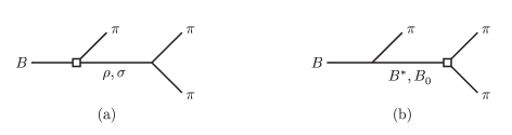
Figure 1: Diagrams contributing to $\,B\to 3\pi,\,$ decay with each square denoting a weak vertex.

III Amplitudes

Practical considerations drive our interest in the $\,\pi^{+}\pi^{-}\pi^{0}$ and $\pi^{\mp}\pi^{\mp}\pi^{\pm}\,$ decay modes; we shall not consider the $\,\pi^{0}\pi^{0}\pi^{\pm}\,$ ones. We write the amplitude for $\,\bar{B}^{0}\to\pi^{+}\bigl{(}p_{+}\bigr{)}\,\pi^{-}\bigl{(}p_{-}\bigr{)}\,\pi^{0}\bigl{(}p_{0}\bigr{)}\,$ decay as a coherent sum of the $\rho$, $\sigma$, $B^{*}$, and $B_{0}$ amplitudes, namely,

$$A^{+-0}\,=\,A_{\rho}^{+-0}+A_{\sigma}^{+-0}+A_{B^{*}}^{+-0}+A_{B_{0}}^{+-0}\;.$$ (15)

For $\,B^{-}\to\pi^{-}\bigl{(}p_{1}\bigr{)}\,\pi^{-}\bigl{(}p_{2}\bigr{)}\,\pi^{+}\bigl{(}p_{+}\bigr{)},\,$ the amplitude $A^{--+}$ can be constructed in an analogous manner.

We consider first the $\,B\to\rho\pi\to 3\pi\,$ contributions, represented by the diagram denoted by “$\rho$” in Fig. 1(a). For each $\rho^{i}$ diagram and $3\pi$ state, the amplitude is written as a product of an amplitude for the $\,B\to\rho^{i}\pi^{j}\,$ weak transition and a vertex function $\Gamma_{\rho\pi\pi}$ describing the $\,\rho^{i}\to\pi\pi\,$ form factor. Were the $\rho$ a narrow resonance, the Breit-Wigner (BW) form

$$\Gamma_{\rho\pi\pi}^{\rm BW}(s)\,=\,{g_{\rho}\over s-M_{\rho}^{2}+{\rm i}\Gamma_{\rho}M_{\rho}}\,\,$$ (16)

would suffice, where $\sqrt{s}$ is the invariant mass of the $2\pi$ system and $g_{\rho}$ is the $\,\rho\to\pi\pi\,$ coupling constant. However, since the $\rho$ is not narrow — its width is some $20\%$ of its mass — this form must be generalized to accommodate known theoretical constraints over the region in $s$ for which it is appreciable. For example, unitarity and time-reversal invariance compel the phase of $\Gamma_{\rho\pi\pi}(s)$ to be that of $\,L=1$, $I=1\,$ $\pi\pi$ scattering for $\,s\lesssim\bigl{(}M_{\pi}+M_{\omega}\bigr{)}^{2},\,$ for which the scattering is elastic. Moreover, the imaginary part of $\Gamma_{\rho\pi\pi}(s)$ must vanish below physical threshold, $\,s=4M_{\pi}^{2}.\,$ For a detailed discussion with references to earlier work, see Refs. GarOCon1 ; GarMei . Following Ref. GarOCon1 , we have

$$\Gamma_{\rho\pi\pi}(s)\,=\,{-F_{\rho}(s)\over f_{\rho\gamma}}\,\,,$$ (17)

where $F_{\rho}(s)$ is the vector form-factor of the pion and $f_{\rho\gamma}$ is the $\rho$-$\gamma$ coupling constant. The parameters in $F_{\rho}(s)$ are determined by fitting to $\,e^{+}e^{-}\to\pi^{+}\pi^{-}\,$ data; what is important is that the parametrization itself is consistent with theoretical constraints. The value of $f_{\rho\gamma}$ is determined from the $\,\rho\to e^{+}e^{-}\,$ width, which, in turn, is extracted from the $\,e^{+}e^{-}\to\pi^{+}\pi^{-}\,$ cross section at $\,s=M_{\rho}^{2}\,$ GarOCon1 ; GarOCon2 . The overall sign is chosen so that Eq. (17) is equivalent to the BW form, Eq. (16), as $\,s\to M_{\rho}^{2}\,$. At $\,s=M_{\rho}^{2}\,$ the BW form is compatible with the various theoretical constraints. In our numerical analysis, we adopt the “solution $B$” fit of Ref. GarOCon1 for $F_{\rho}$, for which $\,f_{\rho\gamma}=0.122\pm 0.001\,\rm GeV^{2}\,$ GarOCon2 . Alternatively, a BW form with a running width $\Gamma_{\rho}(s)$, chosen to be compatible with the form of the $\pi\pi$ phase shift (in the crossed channel) as $\,s\to 4M_{\pi}^{2},\,$ is given in Ref. babarbook . However, the numerical differences between this form and the one we have chosen are small GarMei .

For the decay amplitudes, after summing over the $\rho$ polarizations, we find

$$\begin{array}[]{c}\displaystyle A_{\rho}^{+-0}\,=\,\eta^{-}\,\bigl{(}s_{+-}-s_{+0}\bigr{)}\,\Gamma_{\rho\pi\pi}\bigl{(}s_{-0}\bigr{)}\,+\,\eta^{+}\,\bigl{(}s_{-0}-s_{+-}\bigr{)}\,\Gamma_{\rho\pi\pi}\bigl{(}s_{+0}\bigr{)}\,-\,\eta^{0}\,\bigl{(}s_{-0}-s_{+0}\bigr{)}\,\Gamma_{\rho\pi\pi}\bigl{(}s_{+-}\bigr{)}\,\,,\vspace{2ex}\\ \displaystyle A_{\rho}^{--+}\,=\,-\bar{\eta}^{0}\,\Bigl{[}\bigl{(}s_{12}-s_{1+}\bigr{)}\,\Gamma_{\rho\pi\pi}\bigl{(}s_{2+}\bigr{)}\,+\,\bigl{(}s_{12}-s_{2+}\bigr{)}\,\Gamma_{\rho\pi\pi}\bigl{(}s_{1+}\bigr{)}\Bigr{]}\,\,,\end{array}$$ (20)

where $\,s_{kl}\equiv\bigl{(}p_{k}+p_{l}\bigr{)}^{2},\,$ with

$$\begin{array}[]{c}\displaystyle\eta^{-}\,=\,{G_{\rm F}\over\sqrt{2}}\left(\lambda_{u}\,a_{1}-\lambda_{t}\,a_{4}\right)f_{\rho}\,F_{1}^{B\pi}\,\,,\hskip 20.00003pt\eta^{+}\,=\,{G_{\rm F}\over\sqrt{2}}\left[\lambda_{u}\,a_{1}-\lambda_{t}\left(a_{4}-a_{6}\,R_{q}\right)\right]f_{\pi}M_{\rho}\,A_{0}^{B\rho}\,\,,\vspace{2ex}\\ \displaystyle\eta^{0}\,=\,{-G_{\rm F}\over 2\sqrt{2}}\left\{\left[\lambda_{u}\,a_{2}+\lambda_{t}\left(a_{4}-a_{6}\,R_{q}\right)\right]f_{\pi}M_{\rho}\,A_{0}^{B\rho}\,+\,\left(\lambda_{u}\,a_{2}+\lambda_{t}\,a_{4}\right)f_{\rho}\,F_{1}^{B\pi}\right\}\,\,,\vspace{2ex}\\ \displaystyle\bar{\eta}^{0}\,=\,{G_{\rm F}\over 2}\left\{\left[\lambda_{u}\,a_{1}-\lambda_{t}\left(a_{4}-a_{6}\,R_{q}\right)\right]f_{\pi}M_{\rho}\,A_{0}^{B\rho}\,+\,\left(\lambda_{u}\,a_{2}+\lambda_{t}\,a_{4}\right)f_{\rho}\,F_{1}^{B\pi}\right\}\,\,.\end{array}$$ (24)

Here $\,A_{0}^{B\rho}\equiv A_{0}^{B\to\rho}\bigl{(}M_{\pi}^{2}\bigr{)}\,$ and $\,F_{1}^{B\pi}\equiv F_{1}^{B\to\pi}\bigl{(}M_{\rho}^{2}\bigr{)},\,$ whereas $\,R_{q}\equiv M_{\pi}^{2}/\bigl{[}\bigl{(}m_{b}+\hat{m}\bigr{)}\hat{m}]\,$ — note that we work in the isospin-symmetric limit, for which $\,\hat{m}=m_{u}=m_{d}\,$. The relative signs between the different terms in Eq. (20) follow from the $\rho\pi\pi$ couplings

$$\begin{array}[]{c}\displaystyle\bigl{\langle}\pi^{0}\bigl{(}p_{0}\bigr{)}\,\pi^{\pm}\bigl{(}p_{\pm}\bigr{)}\big{|}\rho^{\pm}\bigr{\rangle}\,=\,\pm g_{\rho}\,\varepsilon_{\rho}\cdot\bigl{(}p_{\pm}-p_{0}\bigr{)}\,\,,\vspace{2ex}\\ \displaystyle\bigl{\langle}\pi^{+}\bigl{(}p_{+}\bigr{)}\,\pi^{-}\bigl{(}p_{-}\bigr{)}\big{|}\rho^{0}\bigr{\rangle}\,=\,g_{\rho}\,\varepsilon_{\rho}\cdot\bigl{(}p_{-}-p_{+}\bigr{)}\,\,,\end{array}$$ (27)

which follow, in turn, from the phase conventions we have chosen for the flavor wave functions: $\,\bigl{|}\pi^{\pm}\bigr{\rangle}=\mp\bigl{|}I=1,I_{3}=\pm 1\bigr{\rangle}\,$ and $\,\bigl{|}\pi^{0}\bigr{\rangle}=\bigl{|}I=1,I_{3}=0\bigr{\rangle},\,$ and similarly for the $\rho$ states. Our $A_{\rho}$ amplitudes agree with those of earlier calculations ali ; dea&co ; GarMei .

We turn next to the $\sigma$ “meson” contributions, represented by the diagram denoted by “$\sigma$” in Fig. 1(a). We use the $\sigma$ to denote a two-pion state with total isospin $\,I=0\,$ and total angular-momentum $\,J=0\,$; it need not be a “pre-existing” resonance, but, rather, can be generated dynamically by the strong pionic final-state interactions in this channel OO . The peak of the broad enhancement associated with the $\sigma$ is close to the $\rho$ in mass, so that the decay $\,B\to\sigma\pi\to 3\pi\,$ can populate the $\,B\to\rho\pi\,$ phase space DeaPol . As in the $\rho$ case, the amplitudes for $\,B\to\sigma\pi\to 3\pi\,$ decays are written as a product of an amplitude for the $\,B\to\sigma\pi$ weak transition and a vertex function $\Gamma_{\sigma\pi\pi}$ describing the $\,\sigma\to\pi\pi\,$ form factor. We write GarMei

$$\Gamma_{\sigma\pi\pi}(s)\,=\,\chi\,\Gamma_{1}^{n*}(s)\,\,,$$ (28)

where $\Gamma_{1}^{n}$ is defined as

$$\bigl{\langle}0\bigr{|}\bar{d}d\bigl{|}\pi^{+}(p_{+})\pi^{-}(p_{-})\bigr{\rangle}\,=\,\sqrt{2\over 3}\,{\Gamma_{1}^{n}(s_{+-})\,B_{0}}\,\,.$$ (29)

We note that $\,B_{0}\equiv M_{\pi}^{2}/(2\hat{m})\,$ is the vacuum quark condensate and $\chi$ is a normalization constant, to be discussed shortly. For our numerical work in the next section, we adopt the $\Gamma_{1}^{n}(s)$ as derived in Ref. MeiOll , after Refs. npa ; basde ; OO . The calculated form factor is realized in a chiral, unitarized, coupled-channel approach; at low energies, the form factor is matched to the one-loop-order expression in chiral perturbation theory GasLeu ; MeiOll . The resulting form factor is consistent with low-energy constraints and is comparable to the scalar form-factor which emerges from the dispersion analysis of Ref. DGL ; however, it is notably different from the Breit-Wigner form adopted in Refs. e791 ; DeaPol to study the role of the $\sigma$ in $B$ and $D$ decays into the $3\pi$ final state. That is,

$$\Gamma_{\sigma\pi\pi}^{\rm BW}(s)\;=\;{g_{\sigma\pi\pi}\over s-M_{\sigma}^{2}+{\rm i}\Gamma_{\sigma}(s)\,M_{\sigma}}\,\,,\,\,\,\quad\Gamma_{\sigma}(s)=\frac{M_{\sigma}\Gamma_{\sigma}}{\sqrt{s}}\sqrt{s-4M_{\pi}^{2}\over M_{\sigma}^{2}-4M_{\pi}^{2}}\;,$$ (30)

where the coupling $\,g_{\sigma\pi\pi}\equiv\langle\pi^{+}\pi^{-}|\sigma\rangle\,$ is determined from the $\,\sigma\to\pi\pi\,$ decay rate. For $\,B\to 3\pi\,$ decay, the numerical changes arising from the use of $\Gamma_{\sigma\pi\pi}(s)$ in place of the BW expression are significant GarMei , as we will see here as well. We determine the normalization $\chi$ by requiring that GarMei

$$\chi\left|\Gamma_{1}^{n}\bigl{(}M_{\sigma}^{2}\bigr{)}\right|\,=\,{g_{\sigma\pi\pi}\over\Gamma_{\sigma}\bigl{(}M_{\sigma}^{2}\bigr{)}\,M_{\sigma}}\,\,,$$ (31)

which equates $\bigl{|}\Gamma_{\sigma\pi\pi}(s)\bigr{|}$ to its BW counterpart at $\,s=M_{\sigma}^{2}.\,$ The values of $M_{\sigma}$ and $\Gamma_{\sigma}$ are extracted from fits of $\Gamma_{\sigma\pi\pi}^{\rm BW}(s)$ to $\,D\to 3\pi\,$ decays e791 . The normalization condition is motivated by noting that the modulus of $\Gamma_{1}^{n}(s)$ is peaked near $\,s=M_{\sigma}^{2},\,$ whereas the normalization of $\Gamma_{1}^{n}(s)$ is sensitive to the values of certain, poorly known low-energy constants GarMei . We emphasize that $M_{\sigma}$ and $\Gamma_{\sigma}$ appear merely in the normalization of $\Gamma_{\sigma\pi\pi}$.

The resulting decay amplitudes are then

$$A_{\sigma}^{+-0}\,=\,\eta_{\sigma}^{0}\,\Gamma_{\sigma\pi\pi}\bigl{(}s_{+-}\bigr{)}\,\,,\hskip 20.00003ptA_{\sigma}^{--+}\,=\,\bar{\eta}_{\sigma}^{0}\left(\Gamma_{\sigma\pi\pi}\bigl{(}s_{1+}\bigr{)}+\Gamma_{\sigma\pi\pi}\bigl{(}s_{2+}\bigr{)}\right)\,\,,$$ (32)

where

$$\begin{array}[]{c}\displaystyle\eta_{\sigma}^{0}\,=\,{G_{\rm F}\over 2}\left\{\left[\lambda_{u}\,a_{2}+\lambda_{t}\left(a_{4}-a_{6}\,R_{q}\right)\right]\left(M_{B}^{2}-M_{\sigma}^{2}\right)f_{\pi}F_{0}^{B\sigma}\,-\,\lambda_{t}\,a_{6}\,{2\langle\sigma|\bar{d}d|0\rangle\over m_{b}-\hat{m}}\left(M_{B}^{2}-M_{\pi}^{2}\right)F_{0}^{B\pi}\right\},\vspace{2ex}\\ \displaystyle\bar{\eta}_{\sigma}^{0}\,=\,{G_{\rm F}\over\sqrt{2}}\left\{\left[\lambda_{u}\,a_{1}-\lambda_{t}\left(a_{4}-a_{6}\,R_{q}\right)\right]\left(M_{B}^{2}-M_{\sigma}^{2}\right)f_{\pi}F_{0}^{B\sigma}\,+\,\lambda_{t}\,a_{6}\,{2\langle\sigma|\bar{d}d|0\rangle\over m_{b}-\hat{m}}\left(M_{B}^{2}-M_{\pi}^{2}\right)F_{0}^{B\pi}\right\},\end{array}$$ (35)

with $\,F_{0}^{B\pi}\equiv F_{0}^{B\to\pi}\bigl{(}M_{\sigma}^{2}\bigr{)}\,$ and $\,F_{0}^{B\sigma}\equiv F_{0}^{B\to\sigma}\bigl{(}M_{\pi}^{2}\bigr{)}.\,$ From Eqs. (28) and (29), it follows that $\,\langle\sigma|\bar{d}d|0\rangle=M_{\pi}^{2}/\bigl{(}\sqrt{6}\,\chi\hat{m}\bigr{)}.\,$ We agree with the weak amplitudes of Ref. GarMei , but disagree with those of Ref. DeaPol in that our $\eta_{\sigma}^{0}$ and $\bar{\eta}_{\sigma}^{0},\,$ neglecting penguin terms, are smaller and larger, respectively, than theirs by a factor of $\sqrt{2}$.

We now evaluate the $B^{*}$ and $B_{0}$ contributions, whose diagrams are shown in Fig. 1(b); we suppose that other excited $B$-meson states could also contribute, but we expect that their larger masses ought to make them less important dea&co . Presently, no reliable data exist on the widths of these heavy mesons, so that their values have to be calculated. Recent estimates B-review ; BecLey suggest that the $B^{*}$ is a very narrow resonance, whereas the $B_{0}$ is less so, its width being some $6\%$ of its mass. Nevertheless, the resonances are sufficiently narrow that it is reasonable to adopt a Breit-Wigner representation for the propagators of these mesons, as in Ref. dea&co . In the combined heavy-quark and chiral limit hq , the strong couplings connecting the $\bigl{(}B^{*},B_{0}\bigr{)}$, $B$, and $\pi$ mesons are dea&co ; B-review ; B0

$$\bigl{\langle}B^{-}\bigl{(}p^{\prime}\bigr{)}\pi^{+}(p)\bigr{|}\bar{B}^{*0}(k,\varepsilon)\bigr{\rangle}\,=\,-{2g\,\sqrt{M_{B}M_{B^{*}}}\over f_{\pi}}\,\varepsilon\cdot p\,\,,$$ (36)

$$\bigl{\langle}B^{-}(p^{\prime})\pi^{+}(p)\bigr{|}\bar{B}_{0}^{0}(k)\bigr{\rangle}\,=\,{h\,\sqrt{M_{B}M_{B_{0}}}\over f_{\pi}}\,{k^{2}-M_{B}^{2}\over M_{B_{0}}}\;.$$ (37)

Using isospin symmetry, we derive

$$\bigl{\langle}B^{-}\pi^{+}\bigr{|}\bar{B}^{*0}\bigr{\rangle}\,=\,-\sqrt{2}\,\bigl{\langle}\bar{B}^{0}\pi^{0}\bigr{|}\bar{B}^{*0}\bigr{\rangle}\,=\,\bigl{\langle}\bar{B}^{0}\pi^{-}\bigr{|}B^{*-}\bigr{\rangle}\,\,$$ (38)

and analogous relations for $\bigl{\langle}B\pi\bigr{|}B_{0}\bigr{\rangle}$. We then obtain

$$\begin{array}[]{c}\displaystyle A_{B^{*}}^{+-0}\;=\;{\frac{1}{\sqrt{2}}K\,\Pi\bigl{(}s_{-0},s_{+-}\bigr{)}+K_{1}\,\Pi\bigl{(}s_{-0},s_{+0}\bigr{)}\over s_{-0}-M_{B^{*}}^{2}+{\rm i}\Gamma_{B^{*}}M_{B^{*}}}\,-\,{\frac{1}{\sqrt{2}}K\,\Pi\bigl{(}s_{+-},s_{-0}\bigr{)}\over s_{+-}-M_{B^{*}}^{2}+{\rm i}\Gamma_{B^{*}}M_{B^{*}}}\,\,,\vspace{2ex}\\ \displaystyle A_{B^{*}}^{--+}\,=\,{K\,\Pi\bigl{(}s_{1+},s_{12}\bigr{)}\over s_{1+}-M_{B^{*}}^{2}+{\rm i}\Gamma_{B^{*}}M_{B^{*}}}\,+\,{K\,\Pi\bigl{(}s_{2+},s_{12}\bigr{)}\over s_{2+}-M_{B^{*}}^{2}+{\rm i}\Gamma_{B^{*}}M_{B^{*}}}\,\,,\end{array}$$ (41)

$$\begin{array}[]{c}\displaystyle A_{B_{0}}^{+-0}\,=\,\left({\tilde{K}^{0}+\tilde{K}^{cc}\over s_{-0}-M_{B_{0}}^{2}+{\rm i}\Gamma_{B_{0}}M_{B_{0}}}\,-\,{\tilde{K}^{0}\over s_{+-}-M_{B_{0}}^{2}+{\rm i}\Gamma_{B_{0}}M_{B_{0}}}\right)\frac{\left(M_{B_{0}}^{2}-M_{\pi}^{2}\right)}{\sqrt{2}}\,\,,\vspace{2ex}\\ \displaystyle A_{B_{0}}^{--+}\,=\,\left({\tilde{K}^{0}\over s_{1+}-M_{B_{0}}^{2}+{\rm i}\Gamma_{B_{0}}M_{B_{0}}}\,+\,{\tilde{K}^{0}\over s_{2+}-M_{B_{0}}^{2}+{\rm i}\Gamma_{B_{0}}M_{B_{0}}}\right)\left(M_{B_{0}}^{2}-M_{\pi}^{2}\right)\,\,,\end{array}$$ (44)

where

$$\begin{array}[]{c}\displaystyle K\,=\,-4G_{\rm F}\left[\lambda_{u}\,a_{1}-\lambda_{t}\left(a_{4}-a_{6}\,R_{q}\right)\right]gM_{B^{*}}\sqrt{M_{B}M_{B^{*}}}\,A_{0}^{B^{*}\pi}\,\,,\vspace{2ex}\\ \displaystyle K_{1}\,=\,-2\sqrt{2}\,G_{\rm F}\left[\lambda_{u}\,a_{2}+\lambda_{t}\left(a_{4}-a_{6}\,R_{q}\right)\right]gM_{B^{*}}\sqrt{M_{B}M_{B^{*}}}\,A_{0}^{B^{*}\pi}\,\,,\end{array}$$ (47)

$$\begin{array}[]{c}\displaystyle\tilde{K}^{0}\,=\,{G_{\rm F}\over\sqrt{2}}\left[\lambda_{u}\,a_{1}-\lambda_{t}\left(a_{4}-a_{6}\,R_{q}\right)\right]{M_{B_{0}}^{2}-M_{B}^{2}\over M_{B_{0}}}\,h\,\sqrt{M_{B}M_{B_{0}}}\,F_{0}^{B_{0}\pi}\,\,,\vspace{2ex}\\ \displaystyle\tilde{K}^{cc}\,=\,{G_{\rm F}\over\sqrt{2}}\left[\lambda_{u}\,a_{2}+\lambda_{t}\left(a_{4}-a_{6}\,R_{q}\right)\right]{M_{B_{0}}^{2}-M_{B}^{2}\over M_{B_{0}}}\,\,\sqrt{M_{B}M_{B_{0}}}\,F_{0}^{B_{0}\pi}\,\,,\end{array}$$ (50)

and the sum over $B^{*}$ polarizations yields

$$\Pi(u,v)\,=\,{\bigl{(}M_{B}^{2}-M_{\pi}^{2}-u\bigr{)}\,u\over 4M_{B^{*}}^{2}}\,+\,M_{\pi}^{2}-{v\over 2}\,\,.$$ (51)

Note that $\,A_{0}^{B^{*}\pi}\equiv A_{0}^{B^{*}\to\pi}\bigl{(}M_{\pi}^{2}\bigr{)}\,$ and $\,F_{0}^{B_{0}\pi}\equiv F_{0}^{B_{0}\to\pi}\bigl{(}M_{\pi}^{2}\bigr{)}.\,$ Our expressions for $A^{+-0}$ in Eqs. (41) and (44) disagree with those in Ref. dea&co in that the factors of $1/\sqrt{2}$ are missing in their formulas, and that the minus sign in the middle of the big brackets in Eq. (44) is opposite to theirs. However, our expressions for $A^{--+}$ in Eqs. (41) and (44) agree with theirs.

IV Numerical results and discussion

We begin by listing the parameters that we use; we conform with the parameter choices of Refs. dea&co ; GarMei , in order to realize a crisp comparison with their results. In specific, the Wilson coefficients we use are

$$\begin{array}[]{c}\displaystyle C_{1}\,=\,1.100\,,\hskip 5.0ptC_{2}\,=\,-0.226\,,\hskip 5.0ptC_{3}\,=\,0.012\,,\hskip 5.0ptC_{4}\,=\,-0.029\,,\hskip 5.0ptC_{5}\,=\,0.009\,,\hskip 5.0ptC_{6}\,=\,-0.033\,.\end{array}$$ (53)

For the CKM factors, we adopt the Wolfenstein parametrization wolfenstein , retaining terms of ${\cal O}\bigl{(}\lambda^{3}\bigr{)}$ in the real part and of ${\cal O}\bigl{(}\lambda^{5}\bigr{)}$ in the imaginary part, to wit,

$$\begin{array}[]{c}\displaystyle V_{ud}\,=\,1-\lambda^{2}/2\,\,,\hskip 5.0ptV_{ub}\,=\,A\lambda^{3}\,\bigl{[}\rho-{\rm i}\eta\,\bigl{(}1-\lambda^{2}/2\bigr{)}\bigr{]}\,\,,\hskip 5.0ptV_{td}\,=\,A\lambda^{3}\,(1-\rho-{\rm i}\eta)\,\,,\hskip 5.0ptV_{tb}\,=\,1\,\,,\end{array}$$ (55)

and using

$$\lambda\,=\,0.2196\,\,,\hskip 20.00003pt\rho\,=\,0.05\,\,,\hskip 20.00003pt\eta\,=\,0.36\,\,,\hskip 20.00003ptA\,=\,0.806\,\,.$$ (56)

For decay constants, light meson masses, and resonance parameters, we have

$$\begin{array}[]{c}\displaystyle f_{\pi}/\sqrt{2}\,=\,92.4\,{\rm MeV}\,\,,\hskip 20.00003ptM_{\pi}\,=\,139.57\,{\rm MeV}\,\,,\vspace{1ex}\\ \displaystyle f_{\rho}\,=\,0.15\,{\rm GeV}^{2}\,\,,\hskip 20.00003ptM_{\rho}\,=\,769.3\,{\rm MeV}\,\,,\hskip 20.00003pt\Gamma_{\rho}\,=\,150\,{\rm MeV}\,\,,\hskip 20.00003ptg_{\rho}\,=\,5.8\,\,,\vspace{1ex}\\ \displaystyle M_{\sigma}\,=\,478\,{\rm MeV}\,\,,\hskip 20.00003pt\Gamma_{\sigma}\,=\,324\,{\rm MeV}\,\,,\hskip 20.00003ptg_{\sigma\pi\pi}\,=\,2.52\,{\rm GeV}\,\,.\end{array}$$ (60)

The decay constants $f_{\pi}$ and $f_{\rho}$ are associated with $\pi^{\pm}$ and $\rho^{\pm}$ decay, respectively. We neglect isospin-violating effects throughout, so that $\,M_{\pi^{\pm}}=M_{\pi^{0}}=M_{\pi},\,$ $\,M_{\rho^{\pm}}=M_{\rho^{0}}=M_{\rho},\,$ as well as $\,M_{\bar{B}^{0}}=M_{B^{-}}=M_{B}.\,$ Moreover, $\,\hat{m}=6\,{\rm MeV}.\,$ The $B^{*}$ and $B$ are degenerate in the heavy-quark limit, so that we neglect their mass difference as well. We also neglect the lifetime difference between the $\bar{B}^{0}$ and $B^{-}$, setting $\,\tau_{\bar{B}^{0}}=\tau_{B^{-}}=\tau_{B}.\,$ For the $B$ and related mesons, we have

$$\begin{array}[]{c}\displaystyle M_{B}\,=\,5.279\,{\rm GeV}\,\,,\hskip 20.00003pt\tau_{B}=1.6\times 10^{-12}\,{\rm s}\,\,,\hskip 20.00003ptm_{b}\,=\,4.6\,{\rm GeV}\,\,,\vspace{1ex}\\ \displaystyle\Gamma_{B^{*}}\,=\,0.2\,{\rm keV}\,\,,\hskip 20.00003ptM_{B_{0}}\,=\,5.697\,{\rm GeV}\,\,,\hskip 20.00003pt\Gamma_{B_{0}}\,=\,0.36\,{\rm GeV}\,\,,\end{array}$$ (63)

and use

$$g\,=\,0.6\,\,,\hskip 30.00005pth\,=\,-0.7\,\,.$$ (64)

The heavy-to-light transition form factors are given by

$$\begin{array}[]{c}\displaystyle A_{0}^{B\rho}\,=\,0.29\,\,,\hskip 20.00003ptF_{0}^{B\pi}\,=\,0.37\,\,,\hskip 20.00003ptF_{1}^{B\pi}\,=\,0.37\,\,,\hskip 20.00003ptF_{0}^{B\sigma}\,=\,0.46\,\,,\vspace{1ex}\\ \displaystyle A_{0}^{B^{*}\pi}\,=\,0.16\,\,,\hskip 20.00003ptF_{0}^{B_{0}\pi}\,=\,-0.19\,\,.\end{array}$$ (67)

Finally, for the vector and scalar form-factors, $\Gamma_{\rho\pi\pi}(s)$ and $\Gamma_{\sigma\pi\pi}(s)$, respectively, we follow the treatment of Ref. GarMei . The $F_{\rho}(s)$ parametrization we adopt was fit to $\,e^{+}e^{-}\to\pi^{+}\pi^{-}\,$ data in the elastic region GarOCon1 , $\,2M_{\pi}\leq\sqrt{s}\leq M_{\pi}+M_{\omega},\,$ only, so that for larger values of $s$ we use a Breit-Wigner form, matched to the value of $\Gamma_{\rho\pi\pi}(s)$ at $\,\sqrt{s}=M_{\pi}+M_{\omega}.\,$ That is, for $\,\sqrt{s}\gtrsim 923\,\rm MeV\,$ we employ $\,\Gamma_{\rho\pi\pi}(s)=\bigl{[}c_{\rm r}\,\bigl{(}M_{\rho}^{2}-s\bigr{)}+{\rm i}c_{\rm i}\Gamma_{\rho}M_{\rho}\bigr{]}g_{\rho}/\bigl{[}\bigl{(}M_{\rho}^{2}-s\bigr{)}^{2}+\Gamma_{\rho}^{2}M_{\rho}^{2}\bigr{]},\,$ with $\,c_{\rm r}\simeq 0.929\,$ and $\,c_{\rm i}\simeq 1.29.\,$ For the scalar form-factor, we employ the $\Gamma_{1}^{n}(s)$ derived in Ref. MeiOll , which is valid for $\,\sqrt{s}\lesssim 1.2\,\rm GeV.\,$ The normalization of Eq. (31) implies that $\,\chi=20.0\,{\rm GeV}^{-1}.\,$ For $\,\sqrt{s}>1.2\,\rm GeV,\,$ we match to the asymptotic form of $\Gamma_{\sigma\pi\pi}(s)\,$ DGL , as detailed in Ref. GarMei .

To obtain branching ratios for $\,B\to 3\pi\,$ decay in the $\rho$-mass region, we integrate over the region of phase space satisfying the requirement that two of the three pions reconstruct the $\rho$ mass within an interval of 2$\delta$, as was done in Refs. dea&co ; GarMei . This amounts in each case to calculating the effective width

$$\begin{array}[]{c}\displaystyle\Gamma_{\rm eff}\bigl{(}B\to\rho(p_{1}+p_{2})\pi(p_{3})\bigr{)}\,=\,\Gamma\bigl{(}B\to\pi(p_{1})\pi(p_{2})\pi(p_{3})\bigr{)}\Bigl{|}_{(M_{\rho}-\delta)^{2}\leq s_{12}\leq(M_{\rho}+\delta)^{2}}\,\,.\end{array}$$ (69)

We choose $\,\delta=0.3\,\rm GeV,\,$ following earlier work dea&co ; GarMei .

For crisp comparison with Ref. dea&co , we begin by computing the effective branching ratios arising from the use of Breit-Wigner forms, as in Eqs. (16) and (30) for the $\rho$ and $\sigma$, respectively, throughout. The various contributions, reflective of the enumerated terms in Eq. (15), are reported in Table 1. There are differences between our results for the $\rho$, $\,\rho$$+$$B^{*}\,$, and $\,\rho$$+$$B^{*}$$+$$B_{0}\,$ contributions and the corresponding ones in Ref. dea&co . The differences are, however, not large and arise in part from missing factors in the formulas for the $B^{*}$ and $B_{0}$ amplitudes, which we delineated in the last section. In contrast, as pointed out in Ref. GarMei , the $\sigma$ effect on the $B^{-}$ decay is much bigger than that found in Ref. DeaPol , because our $\sigma$ amplitude is larger than theirs by a factor of $\sqrt{2}$. This is evident in the $\,\rho$$+$$\sigma\,$ and $\,\rho$$+$$\sigma$$+$$B^{*}\,$ columns. Our results agree with those Ref. GarMei , to the extent that they are applicable; we note that Ref. GarMei neglects penguin contributions altogether and deals exclusively with the $\rho$ and $\sigma$ contributions. The last column of Table 1 contains the sum of all the contributions, $\,\rho$$+$$\sigma$$+$$B^{*}$$+$$B_{0}\,$. Overall, it is apparent that the effect of the $B_{0}$ is smaller than that of the other contributions, although it is not negligible. Finally, in the last row, we collect the ratios of branching ratios ${\cal R}$ defined in Eq. (1). These results show that the inclusion of the $\sigma$ and $B^{*}$, either individually or together, makes the estimated value of $\cal R$ consistent with the empirical one, given its large error.

Table 1: Effective branching ratios for $\,B\to\rho\pi\,$ decays, as per Eq. (69), with $\,\delta=0.3\,\rm GeV.\,$ Breit-Wigner form factors are used throughout, noting Eqs. (16) and (30) for the $\rho$ and $\sigma$ contributions, respectively. All branching ratios are reported in units of $10^{-6}$.

Decay mode	$\vphantom{\biggl{|}}\rho$	$\sigma$	$B^{*}$	$B_{0}$	$\rho+B^{*}$	$\rho+B^{*}+B_{0}$	$\rho+\sigma$	$\rho+\sigma+B^{*}$	$\rho+\sigma+B^{*}+B_{0}$
$\begin{array}[]{rcl}\displaystyle\bar{B}^{0}&\rightarrow&\rho^{-}\pi^{+}\\ \bar{B}^{0}&\rightarrow&\rho^{+}\pi^{-}\\ \bar{B}^{0}&\rightarrow&\rho^{0}\pi^{0}\vspace{1.0ex}\\ B^{-}&\rightarrow&\rho^{0}\pi^{-}\vspace{0.8ex}\end{array}$	$\begin{array}[]{c}\displaystyle 16.0\\ 4.76\\ 0.91\vspace{1.0ex}\\ 4.10\vspace{0.8ex}\end{array}$	$\begin{array}[]{c}\displaystyle 0.0003\\ 0.0003\\ 0.045\vspace{1.0ex}\\ 5.18\vspace{0.8ex}\end{array}$	$\begin{array}[]{c}\displaystyle 0.54\\ 0.13\\ 0.39\vspace{1.0ex}\\ 2.71\vspace{0.8ex}\end{array}$	$\begin{array}[]{c}\displaystyle 0.009\\ 0.020\\ 0.016\vspace{1.0ex}\\ 0.107\vspace{0.8ex}\end{array}$	$\begin{array}[]{c}\displaystyle 16.5\\ 4.98\\ 1.43\vspace{1.0ex}\\ 7.42\vspace{0.8ex}\end{array}$	$\begin{array}[]{c}\displaystyle 16.3\\ 4.98\\ 1.29\vspace{1.0ex}\\ 8.45\vspace{0.8ex}\end{array}$	$\begin{array}[]{c}\displaystyle 16.0\\ 4.78\\ 0.93\vspace{1.0ex}\\ 8.83\vspace{0.8ex}\end{array}$	$\begin{array}[]{c}\displaystyle 16.4\\ 5.00\\ 1.59\vspace{1.0ex}\\ 7.67\vspace{0.8ex}\end{array}$	$\begin{array}[]{c}\displaystyle 16.3\\ 5.00\\ 1.43\vspace{1.0ex}\\ 7.92\vspace{0.8ex}\end{array}$
$\vphantom{\Bigl{|}}\cal R$	5.1	-	-	-	2.9	2.5	2.3	2.8	2.7

We now proceed to compute the effective branching ratios with the $\rho$ and $\sigma$ form-factors, Eqs. (17) and (28), which we advocate. These results are presented in Table 2. The results without the $\sigma$ contributions change little, as the vector form-factor is not terribly different from its BW counterpart GarMei . In the presence of the $\sigma$, this similarity persists for the $\bar{B}^{0}$ decays, but, in contrast, the $B^{-}$ branching ratios are significantly increased compared to the corresponding ones in Table 1. This effect also tends to diminish the relative impact of the $B^{*}$ and $B_{0}$ contributions on the $\rho^{0}\pi^{-}$ mode, though the heavy mesons persist in making a substantial impact on the effective branching ratio for the $\rho^{0}\pi^{0}$ mode.

Table 2: Effective branching ratios for $\,B\to\rho\pi\,$ decays, as per Eq. (69), with $\,\delta=0.3\,\rm GeV.\,$ We adopt the $\rho$ and $\sigma$ form factors, Eqs. (17) and (28), respectively, which we have advocated. All branching ratios are reported in units of $10^{-6}$.

Decay mode	$\vphantom{\biggl{|}}\rho$	$\sigma$	$B^{*}$	$B_{0}$	$\rho+B^{*}$	$\rho+B^{*}+B_{0}$	$\rho+\sigma$	$\rho+\sigma+B^{*}$	$\rho+\sigma+B^{*}+B_{0}$
$\begin{array}[]{rcl}\displaystyle\bar{B}^{0}&\rightarrow&\rho^{-}\pi^{+}\\ \bar{B}^{0}&\rightarrow&\rho^{+}\pi^{-}\\ \bar{B}^{0}&\rightarrow&\rho^{0}\pi^{0}\vspace{1.0ex}\\ B^{-}&\rightarrow&\rho^{0}\pi^{-}\vspace{0.8ex}\end{array}$	$\begin{array}[]{c}\displaystyle 16.0\\ 4.76\\ 0.86\vspace{1.0ex}\\ 4.06\vspace{0.8ex}\end{array}$	$\begin{array}[]{c}\displaystyle 0.001\\ 0.001\\ 0.065\vspace{1.0ex}\\ 7.66\vspace{0.8ex}\end{array}$	$\begin{array}[]{c}\displaystyle 0.54\\ 0.13\\ 0.39\vspace{1.0ex}\\ 2.71\vspace{0.8ex}\end{array}$	$\begin{array}[]{c}\displaystyle 0.009\\ 0.020\\ 0.016\vspace{1.0ex}\\ 0.107\vspace{0.8ex}\end{array}$	$\begin{array}[]{c}\displaystyle 16.6\\ 4.90\\ 1.35\vspace{1.0ex}\\ 7.20\vspace{0.8ex}\end{array}$	$\begin{array}[]{c}\displaystyle 16.4\\ 4.93\\ 1.21\vspace{1.0ex}\\ 8.25\vspace{0.8ex}\end{array}$	$\begin{array}[]{c}\displaystyle 15.9\\ 4.80\\ 0.91\vspace{1.0ex}\\ 11.1\vspace{0.8ex}\end{array}$	$\begin{array}[]{c}\displaystyle 16.5\\ 4.94\\ 1.47\vspace{1.0ex}\\ 11.9\vspace{0.8ex}\end{array}$	$\begin{array}[]{c}\displaystyle 16.3\\ 4.98\\ 1.33\vspace{1.0ex}\\ 12.7\vspace{0.8ex}\end{array}$
$\vphantom{\Bigl{|}}\cal R$	5.1	-	-	-	3.0	2.6	1.9	1.8	1.7

Were the heavy-meson contributions to the $\rho^{0}\pi^{0}$ mode seen in Table 2 as large as we have estimated, the impact on the Dalitz-plot analysis to extract $\alpha$ from $\bar{B}^{0}(B^{0})\to\pi^{+}\pi^{-}\pi^{0}$ decays would be significant dea&co . Since the $B^{*}$ and $B_{0}$ masses lie outside the phase-space region of $\,B\to 3\pi,\,$ their effects behave as part of the nonresonant background, but are not uniform and obviously interfere with other contributions. The manner in which the contributions are distributed throughout the Dalitz plot is shown for $\,\bar{B}^{0}\to\pi^{+}\pi^{-}\pi^{0}\,$ decay in Fig. 3; the heavy-meson contributions preferentially populate the edges of the Dalitz plot, in which the $\rho$ contributions lie as well. In $B^{-}\to\pi^{+}\pi^{-}\pi^{-}$ decay, the distribution of the heavy-meson contributions is somewhat more uniform, as illustrated in Fig. 3.

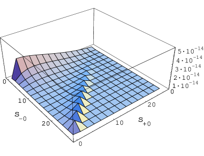
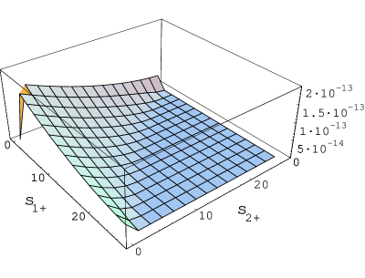
Figure 2: The $B^{*}$ and $B_{0}$ contributions to $\,\bar{B}^{0}\to\pi^{+}(p_{+})\pi^{-}(p_{-})\pi^{0}(p_{0})\,$ decay, specifically, $\bigl{|}A_{B^{*}}^{+-0}+A_{B_{0}}^{+-0}\bigr{|}^{2}$ (in dimensionless units) as a function of its arguments $s_{+0}$ and $s_{-0}$, both in units of GeV².

Figure 3: The $B^{*}$ and $B_{0}$ contributions to $\,B^{-}\to\pi^{-}(p_{1})\pi^{-}(p_{2})\pi^{+}(p_{+})\,$ decay, specifically, $\bigl{|}A_{B^{*}}^{--+}+A_{B_{0}}^{--+}\bigr{|}^{2}$ (in dimensionless units) as a function of its arguments $s_{1+}$ and $s_{2+}$, both in units of GeV².

We now proceed to consider the reliability of the estimates we have effected. Let us first note that the parameters $g$ and $h$ of the strong heavy-meson couplings in Eqs. (36), (37) assume the values given in Eq. (64) — these reflect the upper limits of their estimated ranges dea&co ; B-review . Thus, the results we find with these parameters can be regarded as extremal estimates (although variations in other numerical inputs, such as the form factors, do introduce further uncertainties). Choosing central values of $g$ and $h$ in their estimated ranges decreases the heavy-meson effects by up to some 50$\%\,$ dea&co , as explicitly shown in Table 3.

Table 3: Effective branching ratios for $\,B\to\rho\pi\,$ decays, as in Table 2, except that $\,g=0.40\,$ and $\,h=-0.54\,$ have been used.

Decay mode	$\vphantom{\biggl{|}}\rho$	$B^{*}$	$B_{0}$	$\rho+B^{*}$	$\rho+B^{*}+B_{0}$	$\rho+\sigma$	$\rho+\sigma+B^{*}$	$\rho+\sigma+B^{*}+B_{0}$
$\begin{array}[]{rcl}\displaystyle\bar{B}^{0}&\rightarrow&\rho^{-}\pi^{+}\\ \bar{B}^{0}&\rightarrow&\rho^{+}\pi^{-}\\ \bar{B}^{0}&\rightarrow&\rho^{0}\pi^{0}\vspace{1.0ex}\\ B^{-}&\rightarrow&\rho^{0}\pi^{-}\vspace{0.8ex}\end{array}$	$\begin{array}[]{c}\displaystyle 16.0\\ 4.76\\ 0.86\vspace{1.0ex}\\ 4.06\vspace{0.8ex}\end{array}$	$\begin{array}[]{c}\displaystyle 0.24\\ 0.06\\ 0.17\vspace{1.0ex}\\ 1.20\vspace{0.8ex}\end{array}$	$\begin{array}[]{c}\displaystyle 0.005\\ 0.012\\ 0.009\vspace{1.0ex}\\ 0.064\vspace{0.8ex}\end{array}$	$\begin{array}[]{c}\displaystyle 16.3\\ 4.82\\ 1.10\vspace{1.0ex}\\ 5.55\vspace{0.8ex}\end{array}$	$\begin{array}[]{c}\displaystyle 16.1\\ 4.87\\ 1.03\vspace{1.0ex}\\ 6.12\vspace{0.8ex}\end{array}$	$\begin{array}[]{c}\displaystyle 15.9\\ 4.80\\ 0.91\vspace{1.0ex}\\ 11.1\vspace{0.8ex}\end{array}$	$\begin{array}[]{c}\displaystyle 16.2\\ 4.86\\ 1.20\vspace{1.0ex}\\ 11.0\vspace{0.8ex}\end{array}$	$\begin{array}[]{c}\displaystyle 16.1\\ 4.91\\ 1.13\vspace{1.0ex}\\ 11.4\vspace{0.8ex}\end{array}$
$\vphantom{\Bigl{|}}\cal R$	5.1	-	-	3.8	3.4	1.9	1.9	1.8

Moreover, the relative signs chosen for the $\rho$, $\sigma$, and heavy-meson contributions will impact the numerical values of the effective branching ratios. As noted by Ref. dea&co , the relative sign of the $B^{*}$ and $B_{0}$ contributions is fixed in the heavy-quark and chiral limits. The relative signs of the heavy-meson, $\rho$, and $\sigma$ contributions, however, are less clear. We define the $\rho\to\pi\pi$ coupling as per Eq. (27), after Ref. dea&co ; GarMei , though we note that a chiral Lagrangian analysis suggests that the relations of Eq. (27) should possess an additional overall sign. With this modification, the branching ratios for the $\,\rho$+$B^{*}$+$B_{0}\,$ combination in Table 2 typically become smaller by no more than 15$\%$. However, the $\,\rho$+$\sigma\,$ results in $\,\bar{B}^{0}\to\rho^{0}\pi^{0}\,$ and $\,B^{-}\to\rho^{0}\pi^{-}\,$ become some 3$\%$ and 10$\%$ larger, respectively. The impact on the $\,\rho$+$\sigma$+$B^{*}$+$B_{0}\,$ results is mixed, leading to a suppression of about 10$\%$ in the $\rho^{0}\pi^{0}$ mode and an enhancement of 2$\%$ in the $\rho^{0}\pi^{-}$ mode.

Kinematical cuts can mitigate the impact of the heavy-meson and $\sigma$ contributions. Since the $\rho^{\pm}\pi^{\mp}$ modes are little affected by these notions, we evaluate only the $\rho^{0}\pi^{0}$ and $\rho^{0}\pi^{-}$ modes. We try two different sets of kinematical cuts. For the first one, we set $\,\delta=0.15\,{\rm GeV}=\Gamma_{\rho}\,$ and report our results in Table 5. The relative suppression of the heavy-meson and $\sigma$ contributions is quite modest, if it exists at all. For the second set, we impose not only a $\delta$ cut but also a cut on $\cos\theta$, where $\theta$ is the helicity angle, defined as the angle between the direction of one member of a pion pair from $\rho$ decay and the direction of the parent $B$-meson evaluated in the pair’s rest-frame. Since the $\rho$ contribution has a $\cos^{2}$$\theta$ distribution in $B\to\pi^{+}\pi^{-}\pi^{0}$ decay qui&co , larger values of $|\cos\theta|$ enhance the $\rho$ contribution. Interference effects in the $B^{-}\to\pi^{+}\pi^{-}\pi^{-}$ channel will make this cut less effective. We set $\,\delta=0.3\,\rm GeV\,$ and $\,|\cos\theta|>0.4,\,$ and collect the results in Table 5. Comparing to Table 2, the $\theta$ cut is seen to decrease the relative size of the $\sigma$ background, as discussed in Ref. GarMei . The helicity-angle cut only modestly reduces the $\sigma$ contribution in $\,B^{-}\to\rho^{0}\pi^{-}\,$ decay; however, an assumption of $\rho$ dominance is only needed when one employs an isospin analysis to extract $\sin(2\alpha)$ from $\,B^{0}\bigl{(}\bar{B}^{0}\bigr{)}\to\pi^{+}\pi^{-}\pi^{0}\,$ decay, as detailed in Ref. qui&co . For the $\rho^{0}\pi^{0}$ mode, the chosen cut does significantly reduce an already small contribution. Were the $\sigma$ contribution to the $\rho^{0}\pi^{0}$ mode much larger than we estimate, then a full partial-wave analysis to separate the $s$- and $p$-wave contributions could be both practicable and necessary.

Table 4: Effective branching ratios for $\,B\to\rho\pi\,$ decays, as in Table 2, except that $\,\delta=0.15\,\rm GeV\,$ has been used.

Decay mode	$\vphantom{\biggl{|}}\rho$	$\sigma$	$B^{*}$	$\rho+B^{*}$	$\rho+B^{*}+B_{0}$	$\rho+\sigma$	$\rho+\sigma+B^{*}$	$\rho+\sigma+B^{*}+B_{0}$
$\begin{array}[]{rcl}\displaystyle\bar{B}^{0}&\rightarrow&\rho^{0}\pi^{0}\vspace{1.0ex}\\ B^{-}&\rightarrow&\rho^{0}\pi^{-}\vspace{0.8ex}\end{array}$	$\begin{array}[]{c}\displaystyle 0.33\vspace{1.0ex}\\ 3.36\vspace{0.8ex}\end{array}$	$\begin{array}[]{c}\displaystyle 0.029\vspace{1.0ex}\\ 3.46\vspace{0.8ex}\end{array}$	$\begin{array}[]{c}\displaystyle 0.20\vspace{1.0ex}\\ 1.38\vspace{0.8ex}\end{array}$	$\begin{array}[]{c}\displaystyle 0.55\vspace{1.0ex}\\ 4.82\vspace{0.8ex}\end{array}$	$\begin{array}[]{c}\displaystyle 0.49\vspace{1.0ex}\\ 5.39\vspace{0.8ex}\end{array}$	$\begin{array}[]{c}\displaystyle 0.36\vspace{1.0ex}\\ 6.46\vspace{0.8ex}\end{array}$	$\begin{array}[]{c}\displaystyle 0.59\vspace{1.0ex}\\ 7.56\vspace{0.8ex}\end{array}$	$\begin{array}[]{c}\displaystyle 0.53\vspace{1.0ex}\\ 8.17\vspace{0.8ex}\end{array}$

Table 5: Effective branching ratios for $\,B\to\rho\pi\,$ decays, as in Table 2, but with the additional kinematical cut $\,|\cos\theta|>0.4\,$ as explained in the text.

Decay mode	$\vphantom{\biggl{|}}\rho$	$\sigma$	$B^{*}$	$\rho+B^{*}$	$\rho+B^{*}+B_{0}$	$\rho+\sigma$	$\rho+\sigma+B^{*}$	$\rho+\sigma+B^{*}+B_{0}$
$\begin{array}[]{rcl}\displaystyle\bar{B}^{0}&\rightarrow&\rho^{0}\pi^{0}\vspace{1.0ex}\\ B^{-}&\rightarrow&\rho^{0}\pi^{-}\vspace{0.8ex}\end{array}$	$\begin{array}[]{c}\displaystyle 0.84\vspace{1.0ex}\\ 3.81\vspace{0.8ex}\end{array}$	$\begin{array}[]{c}\displaystyle 0.039\vspace{1.0ex}\\ 4.79\vspace{0.8ex}\end{array}$	$\begin{array}[]{c}\displaystyle 0.27\vspace{1.0ex}\\ 1.71\vspace{0.8ex}\end{array}$	$\begin{array}[]{c}\displaystyle 1.22\vspace{1.0ex}\\ 5.92\vspace{0.8ex}\end{array}$	$\begin{array}[]{c}\displaystyle 1.11\vspace{1.0ex}\\ 6.58\vspace{0.8ex}\end{array}$	$\begin{array}[]{c}\displaystyle 0.87\vspace{1.0ex}\\ 7.97\vspace{0.8ex}\end{array}$	$\begin{array}[]{c}\displaystyle 1.29\vspace{1.0ex}\\ 8.63\vspace{0.8ex}\end{array}$	$\begin{array}[]{c}\displaystyle 1.18\vspace{1.0ex}\\ 9.13\vspace{0.8ex}\end{array}$

Finally, we must discuss a tacit assumption we have made in the estimation of the $B^{*}$ and $B_{0}$ contributions, which is made in Ref. dea&co as well. That is, in realizing the diagrams of Fig. 1(b), we have treated the strong $\bigl{(}B^{*},B_{0}\bigr{)}B\pi$ and weak $\,\bigl{(}B^{*},B_{0}\bigr{)}\to\pi\pi\,$ vertices as if the $B^{*}$ and $B_{0}$ mesons were on their mass shell. This assumption is compatible with the assumed use of the combined heavy-quark and chiral limits in the treatment of the strong $\bigl{(}B^{*},B_{0}\bigr{)}B\pi$ vertices. However, neither assumption is appropriate for $\,B\to\rho\pi\,$ decay. That is, for the $\,B\to 3\pi\,$ decays of interest, we require that two of the three pions have an invariant mass $\sqrt{s}$ comparable to that of the $\rho$ meson. This implies that in most of the relevant phase-space region the mediating heavy-mesons carry $s$ values much smaller than their squared masses — they are highly off-mass-shell. Moreover, the bachelor $\pi$ is never soft in this kinematical region. Thus the combined heavy-quark and chiral limits are used beyond their range of validity. These effects modify the vertices we have assumed in Eqs. (36), (37) and Eq. (14). Unfortunately, the needed off-shell extrapolations cannot be done reliably, although we would generically expect this effect to suppress the numerical importance of the $B^{*}$ and $B_{0}$ contributions. For example, the form factors of Eqs. (14) now depend on both $q^{2}$ and $k^{2}$; the vertices are only “half” off-shell, so that $p^{2}$ does not enter, as the final-state $\pi$ is on its mass shell. Moreover, additional form factors appear. To illustrate, we note that the general parametrization

$$\bigl{\langle}\pi^{+}(p)\bigr{|}\bar{u}\gamma^{\mu}Lb\bigl{|}\bar{B}_{0}^{0}(k)\bigr{\rangle} = -{\rm i}F_{0}^{B_{0}\to\pi}\bigl{(}k^{2},p^{2},q^{2}\bigr{)}\frac{\left(M_{B_{0}}^{2}-M_{\pi}^{2}\right)q^{\mu}}{q^{2}}$$ (70)

$$-\,\,{\rm i}F_{1}^{B_{0}\to\pi}\bigl{(}k^{2},p^{2},q^{2}\bigr{)}\left[p^{\mu}+k^{\mu}-\left(M_{B_{0}}^{2}-M_{\pi}^{2}\right)\frac{q^{\mu}}{q^{2}}\right]$$

predicated by an assumption of Lorentz invariance yields

$$q^{\mu}\bigl{\langle}\pi^{+}(p)\bigr{|}\bar{u}\gamma^{\mu}Lb\bigl{|}\bar{B}_{0}^{0}(k)\bigr{\rangle}\,=\,-{\rm i}\left(M_{B_{0}}^{2}-M_{\pi}^{2}\right)F_{0}^{B_{0}\to\pi}\bigl{(}q^{2},k^{2}\bigr{)}+{\rm i}\left(M_{B_{0}}^{2}-k^{2}\right)F_{1}^{B_{0}\to\pi}\bigl{(}q^{2},k^{2}\bigr{)}$$ (71)

for the half-off-shell matrix element of interest. The matrix element is a linear combination of signed, uncertain contributions, so that its sign is ultimately unclear. Similar considerations apply to the $\,B^{*}\to\pi\,$ matrix element, as well as to the strong vertices of Eqs. (36), (37). In the treatment of Ref. DesEHT , an off-shell extrapolation of Eq. (36), in the kinematic region of interest, is effected through the replacement $\sqrt{M_{B}M_{B^{*}}}\to\sqrt{M_{B}\sqrt{s}}$. To assess the impact of these considerations on the numerical results we have reported, we shall adopt a similarly ad hoc prescription. Thus, we perform the replacement

$$M_{B^{*}}^{3/2}\,\,\to\,\,s^{3/4}\,\,$$ (72)

in the numerator of the $B^{*}$ amplitudes in Eq. (41), so that the “off-shellness” of both the strong and weak vertices is taken into account. We neglect the $B_{0}$ in this simple numerical estimate, as its effect was rather small to start with. We calculate the corresponding branching ratios and collect the results in Table 6. Our simple prescription leads to a dramatic reduction of the $B^{*}$ contributions, as a comparison with Table 2 makes clear. Note that the computed values of ${\cal R}$ are still consistent with the empirical ones, as a reduction in ${\cal R}$ is still realized through the $\sigma$ contributions. Although we cannot draw firm conclusions from this simple exercise, it serves to illustrate that neglecting the off-shell nature of the heavy-meson vertices in the kinematic region of interest could easily lead to a considerable overestimate of their effects.

Table 6: Effective branching ratios for $\,B\to\rho\pi\,$ decays, as in Table 2, except that the off-shellness of the $B^{*}$ meson is included as explained in the text.

Decay mode	$\vphantom{\biggl{|}}\rho$	$\sigma$	$B^{*}$	$\rho+B^{*}$	$\rho+\sigma$	$\rho+\sigma+B^{*}$
$\begin{array}[]{rcl}\displaystyle\bar{B}^{0}&\rightarrow&\rho^{-}\pi^{+}\\ \bar{B}^{0}&\rightarrow&\rho^{+}\pi^{-}\\ \bar{B}^{0}&\rightarrow&\rho^{0}\pi^{0}\vspace{1.0ex}\\ B^{-}&\rightarrow&\rho^{0}\pi^{-}\vspace{0.8ex}\end{array}$	$\begin{array}[]{c}\displaystyle 16.0\\ 4.76\\ 0.86\vspace{1.0ex}\\ 4.06\vspace{0.8ex}\end{array}$	$\begin{array}[]{c}\displaystyle 0.001\\ 0.001\\ 0.065\vspace{1.0ex}\\ 7.66\vspace{0.8ex}\end{array}$	$\begin{array}[]{c}\displaystyle 0.03\\ 0.01\\ 0.02\vspace{1.0ex}\\ 0.25\vspace{0.8ex}\end{array}$	$\begin{array}[]{c}\displaystyle 16.0\\ 4.85\\ 0.88\vspace{1.0ex}\\ 4.43\vspace{0.8ex}\end{array}$	$\begin{array}[]{c}\displaystyle 15.9\\ 4.80\\ 0.91\vspace{1.0ex}\\ 11.1\vspace{0.8ex}\end{array}$	$\begin{array}[]{c}\displaystyle 16.0\\ 4.88\\ 0.95\vspace{1.0ex}\\ 10.7\vspace{0.8ex}\end{array}$
$\vphantom{\Bigl{|}}\cal R$	5.1	-	-	4.7	1.9	1.9

V Conclusions

We have examined resonant and nonresonant backgrounds to $\,B\to\rho\pi\to 3\pi\,$ decays which can potentially impact the extraction of $\alpha$ from a Dalitz-plot analysis of $B\to\pi^{+}\pi^{-}\pi^{0}$ decays qui&co , as well as the value of the ratio of branching ratios we term ${\cal R}$, as defined in Eq. (1). In particular, we have evaluated the effects of nonresonant contributions mediated by the heavy mesons $B^{*}$ and $B_{0}$, as well as the contributions from the light $\sigma$ resonance via $B\to\sigma\pi\to 3\pi$ decay, in the $\rho$-mass region. In this, our analysis parallels that of Refs. dea&co ; DeaPol , though it differs fundamentally in two points. Firstly, we use the vector and scalar form-factors of Ref. GarMei , which are consistent with low-energy theoretical constraints and thus are suitable for the description of broad resonant structures such as the $\rho$ and the $\sigma$. The scalar form factor, in particular, is quite different from the Breit-Wigner form adopted in other analyses DeaPol ; e791 and leads to differing results GarMei . Secondly, in the kinematics of interest, the $B^{*}$ and $B_{0}$ are highly off-mass-shell, impacting the strong and weak vertices which mediate the $\,B\to(B^{*},B_{0})\pi\to\pi\pi\pi\,$ decay. We find that these effects can reduce the heavy-meson contributions substantially.

Our numerical results show, were we to neglect the off-shell effects we have mentioned, that the $B\to\rho^{\pm}\pi^{\mp}$ decay modes are little affected by the $\sigma$ and heavy-meson backgrounds, whereas the $\rho^{0}\pi^{0}$ mode receives large contributions from the latter. In contrast, the $B^{-}\to\pi^{+}\pi^{-}\pi^{-}$ decay mode contains large contributions from both the $\sigma$ and $B^{*}$, though the $\sigma$ contributions numerically dominate. Effecting a simple model of off-shell effects, we find that the $B^{*}$ effects are substantially reduced. The off-shell extrapolation of interest cannot be effected with certainty; nevertheless, our estimates indicate that the neglect of this effect may lead to a substantial overestimate of the $B^{*}$ contributions in $B\to 3\pi$ decay. The role of the $\sigma$ in lowering the theoretical value of ${\cal R}$ and yielding a favorable comparison with experiment persists despite these considerations.

Note added.   Since the submission of this paper for publication, a report by the BABAR Collaboration has appeared B->3pi , giving the experimental bound $\,{\cal B}\bigl{(}B^{\pm}\to\pi^{+}\pi^{-}\pi^{\pm}\bigr{)}<15\times 10^{-6}\,$ at 90% C.L. This can be used to constrain the contribution of the $B^{*}$- and $B_{0}$-pole diagrams. Using the $g$ and $h$ values as in Table 2, we find $\,{\cal B}\bigl{(}B^{-}\to\pi^{+}\pi^{-}\pi^{-})=24.8\times 10^{-6}\,$ for the combined $\,\rho$+$\sigma$+$B^{*}$+$B_{0}\,$ contribution, where we have integrated over all the allowed phase-space. Were we to use the intermediate values of $g$ and $h$ given in Table 3, though such a $g$ is not favored by data D*width , we would obtain $\,{\cal B}\bigl{(}B^{-}\to\pi^{+}\pi^{-}\pi^{-}\bigr{)}=18.7\times 10^{-6}.\,$ If we use our off-shell extrapolation (neglecting the small $B_{0}$ contribution) and the parameters of Table 2, we find $\,{\cal B}\bigl{(}B^{-}\to\pi^{+}\pi^{-}\pi^{-}\bigr{)}=15.4\times 10^{-6}.\,$ This comparison supports our assertion: the treatment of the $B^{*}$ vertices in Ref. dea&co tends to yield an overestimate of their contribution to $\,B\to 3\pi\,$ decay. On a related note, the failure to confront the empirical bound on $\,{\cal B}\bigl{(}B^{-}\to K^{+}K^{-}\pi^{-}\bigr{)}\,$ decay has been described in recent work by Cheng and Yang CheYan .

Acknowledgments   We thank Ulf-G. Meißner for helpful discussions and J.A. Oller for the use of his scalar form factor program. The work of J.T. is supported by the U.S. Department of Energy under contract DE-FG01-00ER45832. S.G. thanks the SLAC Theory Group for hospitality and is supported by the U.S. Department of Energy under contracts DE-FG02-96ER40989 and DE-AC03-76SF00515.

References

(1)
B. Aubert et al. [BABAR Collaboration],
Phys. Rev. Lett. 87, 091801 (2001);
K. Abe et al. [Belle Collaboration],
ibid.87, 091802 (2001).
(2)
See, e.g., Y. Nir, arXiv:hep-ph/0109090;
A.J. Buras, arXiv:hep-ph/0109197.
(3)
N. Cabibbo, Phys. Rev. Lett. 10 (1963) 531;
M. Kobayashi and T. Maskawa,
Prog. Theor. Phys. 49 (1973) 652.
(4)
H.J. Lipkin, Y. Nir, H.R. Quinn, and A. Snyder,
Phys. Rev. D 44, 1454 (1991);
A.E. Snyder and H.R. Quinn, ibid.48, 2139 (1993);
H.R. Quinn and J.P. Silva, ibid.62, 054002 (2000).
(5)
C.P. Jessop et al. [CLEO Collaboration],
Phys. Rev. Lett. 85, 2881 (2000).
(6)
B. Aubert et al. [BABAR Collaboration],
arXiv:hep-ex/0107058.
(7)
Y. Gao and F. Wurthwein [CLEO Collaboration],
arXiv:hep-ex/9904008.
(8)
M. Bauer, B. Stech, and M. Wirbel,
Z. Phys. C 34, 103 (1987).
(9)
A. Deandrea et al., Phys. Rev. D 62, 036001 (2000);
A. Deandrea, arXiv:hep-ph/0005014.
(10)
A. Deandrea and A.D. Polosa, Phys. Rev. Lett. 86, 216 (2001).
(11)
S. Gardner and U.-G. Meißner, hep-ph/0112281, to appear in
Phys. Rev. D.
(12)
G. Buchalla, A.J. Buras, and M.E. Lautenbacher,
Rev. Mod. Phys. 68, 1125 (1996).
(13)
S. Gardner and H.B. O’Connell, Phys. Rev. D 59, 076002 (1999).
(14)
S. Gardner and H.B. O’Connell, Phys. Rev. D 57, 2716 (1998);
ibid.62, 019903(E) (1999).
(15)
P.F. Harrison and H.R. Quinn [BABAR Collaboration],
The BaBar Physics Book, SLAC-R-0504,
http://www.slac.stanford.edu/pubs/slacreports/slac-r-504.html.
(16)
A. Ali, G. Kramer, and C.D. Lu, Phys. Rev. D 58, 094009 (1998).
(17)
J.A. Oller and E. Oset, Phys. Rev. D 60, 074023 (1999).
(18)
U.-G. Meißner and J.A. Oller, Nucl. Phys. A 679, 671 (2001).
(19)
J.A. Oller and E. Oset, Nucl. Phys. A 620, 438 (1997);
ibid.652, 407(E) (1997).
(20)
O. Babelon, J.L. Basdevant, D. Caillerie, and G. Mennessier,
Nucl. Phys. B 113, 445 (1976).
(21) J. Gasser and H. Leutwyler,
Annals Phys. 158, 142 (1984).
(22)
J.F. Donoghue, J. Gasser, and H. Leutwyler,
Nucl. Phys. B 343, 341 (1990).
(23)
E.M. Aitala et al. [E791 Collaboration],
Phys. Rev. Lett. 86, 770 (2001).
(24)
R. Casalbuoni et al., Phys. Rept. 281, 145 (1997);
references therein.
(25)
D. Becirevic and A. Le Yaouanc,
J. High Energy Phys. 9903, 021 (1999).
(26)
G. Burdman and J.F. Donoghue, Phys. Lett. B 280, 287 (1992);
M.B. Wise, Phys. Rev. D 45, 2188 (1992);
T.-M. Yan et al., Phys. Rev. D 46, 1148 (1992);
ibid.55, 5851(E) (1992).
(27)
A.F. Falk, Nucl. Phys. B 378, 79 (1992);
A.F. Falk and M.E. Luke, Phys. Lett. B 292, 119 (1992);
U. Kilian, J.G. Korner, and D. Pirjol,
Phys. Lett. B 288, 360 (1992).
(28)
L. Wolfenstein, Phys. Rev. Lett. 51, 1945 (1983).
(29)
S. Ahmed et al. [CLEO Collaboration],
Phys. Rev. Lett. 87, 251801 (2001).
(30)
N.G. Deshpande, G. Eilam, X.-G. He, and J. Trampetic,
Phys. Rev. D 52, 5354 (1995).
(31)
B. Aubert et al. [BABAR Collaboration], arXiv:hep-ex/0206004.
(32)
H.-Y. Cheng and K.-C. Yang, arXiv:hep-ph/0205133.