Enhanced thermal production of hard dileptons by $3\to 2$ processes

Abstract

In the framework of the Hard Thermal Loop effective theory, we calculate the two-loop contributions to hard lepton pair production in a quark-gluon plasma. We show that the result is free of any infrared and collinear singularity. We also recover the known fact that perturbation theory leads to integrable singularities at the location of the threshold for $q\bar{q}\to\gamma^{*}$. It appears that the process calculated here significantly enhances the rate of low mass hard dileptons.

1. Laboratoire d’Annecy-le-Vieux de Physique Théorique,
   Chemin de Bellevue, B.P. 110,
   74941 Annecy-le-Vieux Cedex, France

2. Laboratoire de Physique Théorique,
   Bât. 210, Université Paris XI,
   91405 Orsay Cedex, France

3. Physics Department and Winnipeg Institute for Theoretical Physics,
   University of Winnipeg,
   Winnipeg, Manitoba R3B 2E9, Canada

LAPTH-908/02, LPT-ORSAY-02/28

1 Introduction

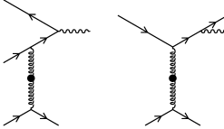
Figure 1: The bremsstrahlung and off-shell annihilation processes that are expected to dominate the production of low mass hard dileptons.

Some time ago a new mechanism for the production of hard photons in a quark-gluon plasma was proposed [1]: the photon is produced by the annihilation of a quark-antiquark pair “after” one of the annihilating quark or antiquark has scattered in the medium (diagram on the right of figure 1). This process is contained in the two-loop diagrams [2, 3] of the Hard Thermal Loop (HTL - [4, 5, 6, 7, 8]) resummed theory. In the HTL approach quarks acquire a thermal mass in the plasma and, at lowest order in the strong coupling, the annihilation of a quark-antiquark pair into a real photon is kinematically forbidden. However when the annihilation is associated to scattering in the plasma one of the quarks becomes off-shell and the annihilation is possible. The interesting feature of the mechanism is that, apart from the exponential suppression factor common to all thermal processes, the photon production rate grows with the energy of the photon, leaving it as the only relevant mechanism when the photon energy is much larger than the temperature. In particular, it dominates over all other processes contained in the one-loop approximation [9, 10, 11, 12, 13, 14] of the HTL approach ($qg\to q\gamma$ and $q\bar{q}\to g\gamma$) which only grow logarithmically with the photon energy. Recent studies, in the framework of the hydrodynamical evolution of the plasma [15, 16, 17, 18, 19], have shown that thermal production of a photon, including the “off-shell annihilation” process, is already significant at SPS energies and could dominate at RHIC and LHC energies. There is then a window, of photon energies of a few GeV, which could provide a signal for the formation of the plasma in heavy ion collisions. However, in this energy range, there is a very large background of pions which decay into photons. Whether the flux of thermal photons can be identified over the large background is under study. In view of this problem it may be useful to consider an alternative signal which follows the same dynamics as real photon production but which suffers from a different experimental background. The production of small mass ($\sqrt{Q^{2}}$) dilepton pairs at relatively hard energy ($q_{0}$) is such a process and this is what is considered below in the limit $\sqrt{Q^{2}}\ll q_{0}$. Considering lepton pair production leads to an interesting situation where two hard scales, $T$ the temperature and $q_{0}$, and three small scales, $\sqrt{Q^{2}}$, $M_{\infty}\sim gT$ the thermal mass of fermions and $m_{\rm g}\sim gT$ the thermal mass of the gluon enter the game. It turns out that several of these scales combine in a single expression $M_{\rm{eff}}$ which acts as a cut-off to regularize potential collinear singularities associated with the fermion propagators. However, in the off-shell annihilation process, $M^{2}_{\rm{eff}}$ can vanish and even become negative. Its role as a cut-off is then blurred! This occurs when the condition

$$Q^{2}>4\ M^{2}_{\infty}$$

is satisfied. In this case, lepton pairs can be produced at ${\cal O}(0)$ in the strong interactions by the annihilation of a $q\bar{q}$ pair, a new feature compared to the case of real photon production. When going to higher orders in the strong interactions it means that two types of diagrams will contribute, which are usually referred to as real and virtual diagrams. This point, which involves the compensation of divergences between the two types of diagrams [20, 21, 22, 23, 24, 25], will be discussed in some details below as it has no equivalent in the case of real photon production. Even after all divergences are cancelled, the dilepton invariant mass spectrum still exhibits an integrable singularity at $Q^{2}=4\ M^{2}_{\infty}$. This is in agreement with a theorem of perturbation theory [26] which states that if an observable has its phase space restricted by a $\theta$ function at a given order of the perturbative expansion, it may exhibit $\delta$ function singularity at the next order.

The collinear enhancement mechanism that makes the processes of figure 1 important has also been shown to play a role in multi-loop diagrams belonging to the class of ladder corrections and self-energy-corrections [27, 28, 29, 30, 31, 32, 33], and a resummation of this family of diagrams has been carried out in [32, 33]. The effect of this resummation, also known as Landau-Pomeranchuk-Migdal (LPM) effect [34, 35, 36], leads to a small reduction (by about 25% for photons in the range interesting for phenomenology) of the photon rate. Assuming that the magnitude of this effect remains comparable for reasonable photon invariant masses (the photon mass helps to regularize the collinear singularities), we limit ourselves to a 2-loop calculation. These contributions add up to the processes $q\bar{q}\to g\gamma^{*}$ and $qg\to q\gamma^{*}$ already calculated in [37, 38].

In the following section, we set up the formalism, then we discuss the matrix element showing, before carrying out the phase space integration, that cancellation of some infra-red divergences can be expected between vertex and self energy diagrams. In Sec. 4 the phase space integration is carried out while in Sec. 5 the behavior of the spectrum near the singular point $Q^{2}=4\ M^{2}_{\infty}$ is studied analytically and found to be in complete agreement with the numerical studies. Finally, Sec. 6 is devoted to some simple phenomenological studies. An appendix contains details of the phase space integration.

In our study on dilepton pair production we rederive, as the limit when the dilepton mass vanishes, the results already obtained on real photon production. The method we follow is however simpler than previously used. It still uses the retarded/advanced (R/A) formalism [39, 13, 40, 41, 42] but it relies on carrying out some integrations in the complex energy plane for which the R/A formalism is well suited. Furthermore, when discussing the compensation of divergences and calculating the remaining finite pieces, there is no need to go to $n-$dimensions or introduce regulators since the compensations can be seen within the integrand.

Some of the results of this paper rely on a new sum-rule presented elsewhere [43], which allows to analytically carry out otherwise difficult numerical integrations.

2 Model

2.1 Formula for the dilepton rate

In a quark-gluon plasma in local thermal equilibrium, the number of lepton pairs produced from virtual photons per unit time and per unit volume is conveniently expressed in terms of the imaginary part of the retarded photon polarization tensor, calculated in presence of the plasma [44, 45]:

$${{dN^{l^{+}l^{-}}}\over{dtd^{3}{\tenimbf x}}}=-{{d\omega d^{3}{\tenimbf q}}\over{12\pi^{4}}}{\alpha\over{Q^{2}}}n_{{}_{B}}(\omega)\,{\rm Im}\,\Pi_{{}_{R}}{}^{\mu}_{\mu}(\omega,{\tenimbf q})\;.$$ (1)

In this formula, the sum over the phase-space of the lepton pair in which the virtual photon decays has been performed, at a fixed total momentum $Q\equiv(\omega,{\tenimbf q})$ of the pair. The trace over the Lorentz indices $\cdots{}^{\mu}_{\mu}$ indicates that both the longitudinal and transverse modes of the massive photon are included. Note that this formula is valid at lowest order in the electromagnetic coupling constant, and at all orders in the strong coupling constant. In more physical terms, it neglects the possible reinteractions of the photon or leptons on their way out of the plasma, and it is valid only if the size of the system is small compared to the mean free path of a photon or lepton.

Another limitation of this formula is that it holds for a plasma in thermal and chemical equilibrium. However, it can also be applied to a situation where there is only a local equilibrium, provided the typical size of the cells over which the system can be considered to be equilibrated is large in front of the photon formation time [30, 46]. If this condition is not satisfied, one has to go back to basics, and use a non-equilibrium real-time formulation in order to compute the rate [47, 48, 49, 50, 51] .

2.2 Hard thermal loops

In order to perform this calculation using thermal field theory, one must resum the bare propagators and vertices in order to account for the fact that medium effects modify the interactions and properties of the excitations of the plasma. In particular, medium induced masses are of utmost importance for quarks in processes where the photon is predominantly produced in a collinear configuration. In thermal field theory, this is achieved through the HTL resummation, which resums an infinite set of one-loop thermal corrections to propagators and vertices.

Since the quarks are always hard in the processes we consider throughout this paper, we keep only the asymptotic thermal mass from the HTL fermionic self-energy [53], which leads to the following retarded and advanced propagators

$$S_{{}_{R,A}}(P)\equiv\overline{\raise 0.6458pt\hbox{$/$}\kern-5.29999pt\hbox{$P$}}s_{{}_{R,A}}(P)\;,$$ (2)

with

$$\overline{P}\equiv(p_{0},\sqrt{{\tenimbf p}^{2}+M_{\infty}^{2}}\hat{\tenimbf p})$$

$$s_{{}_{R,A}}(P)={i\over{P^{2}-M_{\infty}^{2}\pm ip_{0}\epsilon}}\;,$$ (3)

where $M_{\infty}^{2}\equiv g^{2}C_{{}_{F}}T^{2}/4$ is the square of the thermal mass of a hard quark ($C_{{}_{F}}\equiv(N_{c}^{2}-1)/2N_{c}$ is the Casimir in the fundamental representation of the gauge group $SU(N_{c})$). Ordinarily, one does not need effective $\gamma\bar{q}q$ vertices if the quarks are hard, since the HTL corrections are suppressed. But this is correct only if the terms we are calculating are at leading order. Photon production however involves an important cancellation between the components $\Pi_{00}$ and $\Pi_{zz}$ of the photon polarization tensor, and the remaining terms in $\Pi_{\mu}{}^{\mu}$ are non leading, and are affected by the HTL corrections to the vertex. In the following, we do not need the explicit form of the vertex, but only need to know how it is related to the self-energy correction by means of Ward identities. In other words, it is important to make sure that we do for the effective vertex an approximation which is consistent with the approximation of Eq. (3) made for the quark propagator. In particular, we want to preserve the relations satisfied by the full HTL corrections (for a vertex in which a quark enters with momentum $R$ and goes out with momentum $P$):

$$P_{\mu}\delta\Gamma^{\mu}=\raise 0.6458pt\hbox{$/$}\kern-5.29999pt\hbox{$\Sigma$}(R)=\raise 0.6458pt\hbox{$/$}\kern-5.29999pt\hbox{$R$}-\overline{\raise 0.6458pt\hbox{$/$}\kern-5.29999pt\hbox{$R$}}\;,$$

$$R_{\mu}\delta\Gamma^{\mu}=\raise 0.6458pt\hbox{$/$}\kern-5.29999pt\hbox{$\Sigma$}(P)=\raise 0.6458pt\hbox{$/$}\kern-5.29999pt\hbox{$P$}-\overline{\raise 0.6458pt\hbox{$/$}\kern-5.29999pt\hbox{$P$}}\;,$$ (4)

where $\delta\Gamma$ is the HTL correction to the vertex. In the following, it will be useful to write

$$\delta\Gamma^{\mu}\equiv\Gamma^{\mu\nu}\gamma_{\nu}\;.$$ (5)

In addition, we need the effective retarded and advanced propagators of a gluon, which can be decomposed into its transverse and longitudinal components:

$$-D^{\mu\nu}_{{}_{R,A}}(L)\equiv P_{{}_{T}}^{\mu\nu}(L)\Delta_{{}_{R,A}}^{{}^{T}}(L)+P_{{}_{L}}^{\mu\nu}(L)\Delta_{{}_{R,A}}^{{}^{L}}(L)\;,$$ (6)

where $P_{{}_{T,L}}^{\mu\nu}(L)$ are respectively the transverse and longitudinal projectors for a gauge boson of momentum $L$ [54]:

$$P^{\mu\nu}_{{}_{T}}(L)=\gamma^{\mu\nu}-{{\kappa^{\mu}\kappa^{\nu}}\over{\kappa^{2}}}$$

$$P^{\mu\nu}_{{}_{L}}(L)=g^{\mu\nu}-{{L^{\mu}L^{\nu}}\over{L^{2}}}-P_{{}_{T}}^{\mu\nu}(L)\;,$$ (8)

where $\gamma^{\mu\nu}\equiv g^{\mu\nu}-U^{\mu}U^{\nu}$, $\kappa^{\mu}\equiv\gamma^{\mu\nu}L_{\nu}$, and where $U$ is the mean velocity of the plasma in the frame under consideration. The propagators of the transverse and longitudinal modes are then given by

$$\Delta_{{}_{R,A}}^{{}^{T,L}}(L)\equiv{i\over{L^{2}-\Pi_{{}_{R,A}}^{{}^{T,L}}(L)}}\;,$$ (9)

with the following HTL self-energies

$$\Pi^{{}^{T}}(L)=3m_{\rm g}^{2} \left[{{x^{2}}\over 2}+{{x(1-x^{2})}\over{4}}\ln\left({{x+1}\over{x-1}}\right)\right]$$

$$\Pi^{{}^{L}}(L)=3m_{\rm g}^{2} \left[(1-x^{2})-{{x(1-x^{2})}\over{2}}\ln\left({{x+1}\over{x-1}}\right)\right]\;,$$

where we denote $x\equiv l_{0}/l$ and where $m_{\rm g}^{2}\equiv g^{2}T^{2}[N_{c}+N_{{}_{F}}/2]/9$ is the gluon thermal mass in an $SU(N_{c})$ gauge theory with $N_{{}_{F}}$ flavors. Note that an implicit continuation $l_{0}\to l_{0}\pm i\epsilon$ is understood in this self-energy in order to obtain its retarded and advanced components.

3 Matrix element

3.1 Diagrams

Let us now move to the two-loop diagrams calculated in this paper. They are the same as those already considered in [2, 3, 1] for real photons and in [55] for soft dileptons produced at rest in the plasma frame. One of them is a vertex correction to the one-loop photon self-energy, and the other is a self-energy insertion on one of the quarks lines (see figure 2).

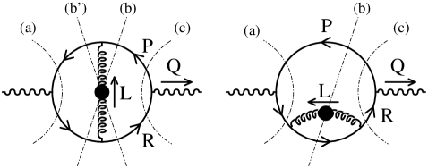
Figure 2: The two-loop diagrams contributing to the production of hard dileptons. A third diagram with a self-energy insertion on the upper quark line is not shown here.

There is however one major difference compared to the case of real photons: as long as the invariant mass of the lepton pair is $Q^{2}<4M_{\infty}^{2}$, the cuts denoted by $(a)$ and $(c)$ in figure 2 do not contribute. Indeed, they correspond to the interference between the tree-level process $q\bar{q}\to\gamma^{*}$ and a virtual correction to this process, but this direct production mechanism has a threshold at $Q^{2}=4M_{\infty}^{2}$. Above the threshold, one must include these cuts, and in fact the various cuts partly compensate each other through the KLN mechanism.

3.2 Vertex contribution

It is convenient to use the retarded-advanced formalism [39, 13, 40, 41, 42] in order to compute the retarded photon polarization tensor needed in Eq. (1). Throughout this paper, we assume that the gluon of momentum $L$ (see diagrams and notations in figure 2) is soft, so that the corresponding Bose-Einstein factor $n_{{}_{B}}(l_{0})$ is large, in particular large compared to fermionic statistical factors. When performing the integrals, one can check the validity of this hypothesis. Therefore, we keep only those terms containing this enhanced Bose-Einstein factor, and we approximate $n_{{}_{B}}(l_{0})\approx T/l_{0}$.

Using this approximation, the contribution of the first diagram (which we designate by “vertex correction” in the following) of figure 2 to the photon polarization tensor is given by:

$${\rm Im}\,\Pi_{{}_{R}}{}_{\mu}^{\mu}(Q)\Big{|}_{\rm vertex}\approx{1\over 2}e^{2}g^{2}N_{c}C_{{}_{F}}\int{{d^{4}P}\over{(2\pi)^{4}}}[n_{{}_{F}}(r_{0})-n_{{}_{F}}(p_{0})]$$

$$\qquad\qquad\qquad\qquad\times\int{{d^{4}L}\over{(2\pi)^{4}}}{T\over{l_{0}}}\sum_{\alpha=T,L}\rho_{\alpha}(L)P_{\alpha}^{\rho\sigma}(L){\rm Trace}^{\rm vert}_{\rho\sigma}$$

$$\qquad\qquad\qquad\qquad\times[s_{{}_{R}}(P)s_{{}_{R}}(P+L)-s_{{}_{A}}(P)s_{{}_{A}}(P+L)]$$

$$\qquad\qquad\qquad\qquad\times[s_{{}_{R}}(R)s_{{}_{R}}(R+L)-s_{{}_{A}}(R)s_{{}_{A}}(R+L)]\;,$$ (11)

where $\rho_{\alpha}(L)$ is the spectral function for the mode $\alpha$ of the effective gluon propagator:

$$\rho_{\alpha}(L)\equiv\Delta_{{}_{R}}^{\alpha}(L)-\Delta_{{}_{A}}^{\alpha}(L)\;,$$ (12)

and where ${\rm Trace}^{\rm vert}_{\rho\sigma}$ denotes the trace of the Dirac matrices for this diagram:

$${\rm Trace}^{\rm vert}_{\rho\sigma}\equiv{\rm Tr}\,[\overline{\raise 0.6458pt\hbox{$/$}\kern-5.29999pt\hbox{$P$}}(\gamma^{\mu}+\delta\Gamma^{\mu})\overline{\raise 0.6458pt\hbox{$/$}\kern-5.29999pt\hbox{$R$}}(\gamma_{\rho}+\delta\Gamma_{\rho})(\overline{\raise 0.6458pt\hbox{$/$}\kern-5.29999pt\hbox{$R$}+\raise 0.6458pt\hbox{$/$}\kern-5.29999pt\hbox{$L$}})(\gamma_{\mu}+\delta\Gamma_{\mu})(\overline{\raise 0.6458pt\hbox{$/$}\kern-5.29999pt\hbox{$P$}+\raise 0.6458pt\hbox{$/$}\kern-5.29999pt\hbox{$L$}})(\gamma_{\sigma}+\delta\Gamma_{\sigma})]\,.$$ (13)

This trace contains four hard momenta, and is a priori of order $T^{4}$ or larger. It is however important to keep also subleading terms of order $T^{2}M_{\infty}^{2}$ since the cancellation between $\Pi_{00}$ and $\Pi_{zz}$ kills all the leading terms when the vertex and self-energy diagrams are combined. However, it is safe to drop all the smaller corrections, i.e. terms of order $M_{\infty}^{4}$ or smaller. Expanding this trace up to terms with two powers of a soft quantity, we find:

$${\rm Trace}^{\rm vert}_{\rho\sigma} \approx -4\Big{[}2(\overline{R}^{2}+(\overline{R+L})^{2})P_{\rho}Q_{\sigma}-2(\overline{P}^{2}+(\overline{P+L})^{2})R_{\rho}Q_{\sigma}$$ (14)

$$\qquad+2L^{2}(R_{\rho}R_{\sigma}+P_{\rho}P_{\sigma})+4(\overline{P}^{2}+\overline{R}^{2})P_{\rho}R_{\sigma}$$

$$\qquad-8(\overline{P}^{\alpha}+\Gamma^{\alpha\beta}P_{\beta})(\overline{R}_{\alpha}+\Gamma_{\alpha}{}^{\gamma}R_{\gamma})P_{\rho}R_{\sigma}$$

$$\qquad-8(Q^{\alpha}+\Gamma^{\alpha\beta}Q_{\beta})(Q_{\alpha}+\Gamma_{\alpha}{}^{\gamma}Q_{\gamma})P_{\rho}R_{\sigma}\Big{]}\;.$$

In this expression, one can even drop the terms with two powers of the vertex correction $\Gamma^{\mu\nu}$, since they would be smaller than the terms we are interested in here. Using the pseudo Ward identities of Eqs. (4), it is possible to rewrite the three terms in $P_{\rho}R_{\sigma}$ as

$$16\left[Q^{2}+2(P\cdot R-\overline{P}\cdot\overline{R})\right]P_{\rho}R_{\sigma}\;,$$ (15)

up to terms that contain more powers of soft factors.

3.3 Self-energy contribution

Similarly, the contribution of the diagram with a self-energy insertion on the quark of momentum $R$ is given by

$${\rm Im}\,\Pi_{{}_{R}}{}_{\mu}^{\mu}(Q)\Big{|}_{\rm self}\approx{1\over 2}e^{2}g^{2}N_{c}C_{{}_{F}}\int{{d^{4}P}\over{(2\pi)^{4}}}[n_{{}_{F}}(r_{0})-n_{{}_{F}}(p_{0})]$$

$$\qquad\qquad\qquad\qquad\times\int{{d^{4}L}\over{(2\pi)^{4}}}{T\over{l_{0}}}\sum_{\alpha=T,L}\rho_{\alpha}(L)P_{\alpha}^{\rho\sigma}(L){\rm Trace}^{\rm self}_{\rho\sigma}$$

$$\qquad\qquad\qquad\qquad\times[s_{{}_{R}}(P)-s_{{}_{A}}(P)]$$

$$\qquad\qquad\qquad\qquad\times[[s_{{}_{R}}(R)]^{2}s_{{}_{R}}(R+L)-[s_{{}_{A}}(R)]^{2}s_{{}_{A}}(R+L)]\;,$$ (16)

where ${\rm Trace}^{\rm self}_{\rho\sigma}$ is the corresponding Dirac trace:

$${\rm Trace}^{\rm self}_{\rho\sigma}\equiv{\rm Tr}\,[\overline{\raise 0.6458pt\hbox{$/$}\kern-5.29999pt\hbox{$P$}}(\gamma^{\mu}+\delta\Gamma^{\mu})\overline{\raise 0.6458pt\hbox{$/$}\kern-5.29999pt\hbox{$R$}}(\gamma_{\rho}+\delta\Gamma_{\rho})(\overline{\raise 0.6458pt\hbox{$/$}\kern-5.29999pt\hbox{$R$}+\raise 0.6458pt\hbox{$/$}\kern-5.29999pt\hbox{$L$}})(\gamma_{\sigma}+\delta\Gamma_{\sigma})\overline{\raise 0.6458pt\hbox{$/$}\kern-5.29999pt\hbox{$R$}}(\gamma_{\mu}+\delta\Gamma_{\mu})]\;.$$ (17)

Calculating this trace down to the order $T^{2}M_{\infty}^{2}$, we obtain

$${\rm Trace}^{\rm self}_{\rho\sigma} \approx -4\Big{[}4\overline{R}^{2}R_{\rho}Q_{\sigma}+4(\overline{P}^{2}+\overline{R}^{2})R_{\rho}R_{\sigma}$$ (18)

$$\qquad-8(\overline{P}^{\alpha}+\Gamma^{\alpha\beta}P_{\beta})(\overline{R}_{\alpha}+\Gamma_{\alpha}{}^{\gamma}R_{\gamma})R_{\rho}R_{\sigma}$$

$$\qquad-8(Q^{\alpha}+\Gamma^{\alpha\beta}Q_{\beta})(Q_{\alpha}+\Gamma_{\alpha}{}^{\gamma}Q_{\gamma})R_{\rho}R_{\sigma}\Big{]}\;.$$

We can recognize the same set of terms as the one evaluated in Eq. (15), with $P_{\rho}R_{\sigma}$ replaced by $R_{\rho}R_{\sigma}$. Of course, there is also another such diagram, not represented explicitly in figure 2, with the self-energy insertion on the quark of momentum $P$. In fact, the contribution of this diagram is equal to that of the first self-energy insertion. Alternatively, the corresponding matrix element can be obtained from the previous one by performing the following change of variables:

$$Q\to Q\;,$$

$$R\to-P\;,$$

$$L\to-L\;.$$ (19)

This second method, compared to the one where we just multiply Eq. (18) by a factor 2, has the advantage of making the matrix element symmetric under the exchange of $P$ and $R$ and is preferred in order to see some cancellations.

3.4 Partial cancellation between vertex and self

Without performing any explicit calculation, one can first prove that the terms in $R_{\rho}Q_{\sigma}$ and $P_{\rho}Q_{\sigma}$ all cancel when one combines the contribution of the vertex correction diagram, and of the two self-energy insertion diagrams. These terms can be rewritten as

$$-2e^{2}g^{2}N_{c}C_{{}_{F}}\int{{d^{4}P}\over{(2\pi)^{4}}}[n_{{}_{F}}(r_{0})-n_{{}_{F}}(p_{0})]$$

$$\qquad\qquad\times\int{{d^{4}L}\over{(2\pi)^{4}}}{T\over{l_{0}}}\sum_{\alpha=T,L}\rho_{\alpha}(L)P_{\alpha}^{\rho\sigma}(L)$$

$$\qquad\qquad\times\Big{[}2(\overline{R}^{2}+(\overline{R+L})^{2})P_{\rho}Q_{\sigma}\;s_{{}_{R}}(P)s_{{}_{R}}(P+L)s_{{}_{A}}(R)s_{{}_{A}}(R+L)$$

$$\qquad\qquad\quad-2(\overline{P}^{2}+(\overline{P+L})^{2})R_{\rho}Q_{\sigma}\;s_{{}_{R}}(P)s_{{}_{R}}(P+L)s_{{}_{A}}(R)s_{{}_{A}}(R+L)$$

$$\qquad\qquad\quad+4\overline{R}^{2}R_{\rho}Q_{\sigma}\;s_{{}_{R}}(P)[s_{{}_{A}}(R)]^{2}s_{{}_{A}}(R+L)$$

$$\qquad\qquad\quad-4\overline{P}^{2}P_{\rho}Q_{\sigma}\;s_{{}_{A}}(R)[s_{{}_{R}}(P)]^{2}s_{{}_{R}}(P+L)\Big{]}+{\rm c.c.}\;.$$ (20)

Using $\overline{P}^{2}s_{{}_{R,A}}(P)=i$, one can check that the square bracket in this equation is proportional to:

$$\Big{[}4P_{\rho}Q_{\sigma}\;s_{{}_{R}}(P)s_{{}_{R}}(P+L)\Big{(}s_{{}_{A}}(R+L)-s_{{}_{A}}(R)\Big{)}$$

$$-4R_{\rho}Q_{\sigma}\;s_{{}_{A}}(R)s_{{}_{A}}(R+L)\Big{(}s_{{}_{R}}(P+L)-s_{{}_{R}}(P)\Big{)}\Big{]}\;.$$ (21)

Assuming that the gluon momentum $L$ is small compared to the quark momenta $P$ and $R$, and performing the change of variables

$$P+L\to-R\;,$$

$$L\to L\;,$$ (22)

on some of the terms (dropping terms in $L_{\rho}$ that may appear), one can observe that the two lines cancel each other. This cancellation is in fact a particular case of a cancellation between ladder diagrams and self-energy insertions discussed in [27, 28, 56, 57, 58, 29, 32, 33]. For the remaining terms, we have:

$${\rm Im}\,\Pi_{{}_{R}}{}_{\mu}^{\mu}(Q)\approx-2e^{2}g^{2}N_{c}C_{{}_{F}}\int{{d^{4}P}\over{(2\pi)^{4}}}[n_{{}_{F}}(r_{0})-n_{{}_{F}}(p_{0})]$$

$$\qquad\times\int{{d^{4}L}\over{(2\pi)^{4}}}{T\over{l_{0}}}\sum_{\alpha=T,L}\rho_{\alpha}(L)P_{\alpha}^{\rho\sigma}(L)$$

$$\qquad\times\Big{[}2L^{2}(R_{\rho}R_{\sigma}+P_{\rho}P_{\sigma})\;s_{{}_{R}}(P)s_{{}_{R}}(P+L)s_{{}_{A}}(R)s_{{}_{A}}(R+L)$$

$$\qquad\quad-4(Q^{2}+2(P\cdot R-\overline{P}\cdot\overline{R}))R_{\rho}P_{\sigma}\;s_{{}_{R}}(P)s_{{}_{R}}(P+L)s_{{}_{A}}(R)s_{{}_{A}}(R+L)$$

$$\qquad\quad-4(Q^{2}+2(P\cdot R-\overline{P}\cdot\overline{R}))R_{\rho}R_{\sigma}\;s_{{}_{R}}(P)[s_{{}_{A}}(R)]^{2}s_{{}_{A}}(R+L)$$

$$\qquad\quad-4(Q^{2}+2(P\cdot R-\overline{P}\cdot\overline{R}))P_{\rho}P_{\sigma}\;s_{{}_{A}}(R)[s_{{}_{R}}(P)]^{2}s_{{}_{R}}(P+L)\Big{]}+{\rm c.c.}\;.$$

(23)

Let us add that, since we are looking at photons whose virtuality is not negligible, we have kept the terms in $Q^{2}$ when they have the collinearly enhanced quark propagators.

4 Integration over the quark momentum

4.1 Pole structure of the integrand and collinear enhancement

We are now in a position to perform the integration over the quark momentum. We perform this integration in the complex plane using the theorem of residues, and we integrate first over the component of the quark momentum which is parallel to the photon momentum, i.e. the z-component.

For each term, we have propagators with a retarded prescription multiplied by propagators with an advanced prescription. It is convenient to perform in the complex plane the integration over the longitudinal components of the quark momenta (the reference direction is the photon momentum), by closing the contour around the upper half-plane. In this approach, the collinear enhancement is due to the fact that in a product like $s_{{}_{R}}(P)s_{{}_{A}}(R)$, there are pairs of poles that are separated by a very small interval and are on opposite sides of the real axis. As a consequence, the real axis is “pinched” by such a pair of poles, leading to a large contribution of the order of the small separation between the poles.

Keeping only the contribution of the pinching pole, $p_{z}=p_{0}+({\tenimbf p}_{\perp}^{2}+M_{\rm eff}^{2})/2p_{0}$, the basic result we need is the following (for $R=P+Q$)

$$\int_{-\infty}^{+\infty}{{dp_{z}}\over{2\pi}}s_{{}_{R}}(P)s_{{}_{A}}(R)F(p_{z})\approx{1\over{2iq_{0}}}{1\over{{\tenimbf p}_{\perp}^{2}+M_{\rm eff}^{2}-i{{p_{0}r_{0}}\over{q_{0}}}\epsilon}}F(p_{0})\;,$$ (24)

where, following [3, 1], we denote

$$M_{\rm eff}^{2}\equiv M_{\infty}^{2}+{{Q^{2}}\over{q_{0}^{2}}}p_{0}r_{0}\;.$$ (25)

This result is valid if the function $F$ is not participating in the collinear enhancement (i.e. is well behaved in the vicinity of the poles of the quark propagator).

4.2 Contribution of the vertex diagram

For the calculation of the first two terms in Eq. (23) (i.e. the terms coming from the vertex correction diagram), we use this method in order to perform the integral over the z-component of the quark momentum in each loop, i.e. respectively $p_{z}$ and $p_{z}+l_{z}$ considered as independent variables. These terms become:

$$\left.{\rm Im}\,\Pi_{{}_{R}}{}_{\mu}^{\mu}(Q)\right|_{\rm vertex}\approx$$

$$\qquad\approx{{e^{2}g^{2}N_{c}C_{{}_{F}}}\over{q_{0}^{2}}}\int{{dp_{0}d^{2}{\tenimbf p}_{\perp}}\over{(2\pi)^{3}}}[n_{{}_{F}}(r_{0})-n_{{}_{F}}(p_{0})]\int{{dl_{0}d^{2}{\tenimbf l}_{\perp}}\over{(2\pi)^{3}}}{T\over{l_{0}}}$$

$$\qquad\times\sum_{\alpha=T,L}\rho_{\alpha}(L)P_{\alpha}^{\rho\sigma}(L)$$

$$\qquad\times\Big{[}L^{2}(R_{\rho}R_{\sigma}+P_{\rho}P_{\sigma})-2(Q^{2}+2(P\cdot R-\overline{P}\cdot\overline{R}))R_{\rho}P_{\sigma}\Big{]}\Big{|}_{\mathrel{\mathop{\kern 0.0ptp_{z}=p_{0}}\limits_{l_{z}=l_{0}}}}$$

$$\qquad\times{1\over{{\tenimbf p}_{\perp}^{2}+M_{\rm eff}^{2}-i{{p_{0}r_{0}}\over{q_{0}}}\epsilon}}\;{1\over{({\tenimbf p}_{\perp}+{\tenimbf l}_{\perp})^{2}+M_{\rm eff}^{2}-i{{p_{0}r_{0}}\over{q_{0}}}\epsilon}}+\,{\rm c.c.}\;.$$ (26)

Next, we need to perform the contractions with the projectors. For any pair of 4-vectors $A_{\mu},B_{\mu}$ taken in the set $\{P_{\mu},R_{\mu}\}$, we have in the collinear limit:

$$A_{\mu}B_{\nu}P_{{}_{T}}^{\mu\nu}(L)=(\hat{\tenimbf l}\cdot{\tenimbf a})(\hat{\tenimbf l}\cdot{\tenimbf b})-({\tenimbf a}\cdot{\tenimbf b})\approx-A_{\mu}B_{\nu}P_{{}_{L}}^{\mu\nu}(L)\;,$$ (27)

where $\hat{\tenimbf l}\equiv{\tenimbf l}/l$. Noticing that all the transverse components of ${\tenimbf p}$ and ${\tenimbf r}$ are much smaller than the longitudinal components due to the collinear enhancement, we have also

$$\hat{\tenimbf l}\cdot{\tenimbf p}\approx p_{0}{{l_{0}}\over{l}}\;,\qquad\hat{\tenimbf l}\cdot{\tenimbf r}\approx r_{0}{{l_{0}}\over{l}}\;,\qquad{\tenimbf p}\cdot{\tenimbf r}\approx p_{0}r_{0}\;,$$ (28)

so that

$$P_{\rho}P_{\sigma}P_{{}_{T}}^{\rho\sigma}(L)\approx-P_{\rho}P_{\sigma}P_{{}_{L}}^{\rho\sigma}(L)\approx p_{0}^{2}\Big{(}{{l_{0}^{2}}\over{l^{2}}}-1\Big{)}\;,$$

$$R_{\rho}R_{\sigma}P_{{}_{T}}^{\rho\sigma}(L)\approx-R_{\rho}R_{\sigma}P_{{}_{L}}^{\rho\sigma}(L)\approx r_{0}^{2}\Big{(}{{l_{0}^{2}}\over{l^{2}}}-1\Big{)}\;,$$

$$P_{\rho}R_{\sigma}P_{{}_{T}}^{\rho\sigma}(L)\approx-P_{\rho}R_{\sigma}P_{{}_{L}}^{\rho\sigma}(L)\approx p_{0}r_{0}\Big{(}{{l_{0}^{2}}\over{l^{2}}}-1\Big{)}\;.$$ (29)

It is convenient to use the variable $x\equiv l_{0}/l$ instead of $l_{0}$ itself. However, since $l_{z}=l_{0}$ and $l^{2}=l_{0}^{2}+{\tenimbf l}_{\perp}^{2}$, the Jacobian of the transformation differs from $1$. A simple calculation gives:

$$\Big{(}1-{{l_{0}^{2}}\over{l^{2}}}\Big{)}{{dl_{0}}\over{l_{0}}}d(l_{\perp}^{2})={{dx}\over x}d(l_{\perp}^{2})\;.$$ (30)

Therefore, this change of variable enables one to absorb all the factors $1-l_{0}^{2}/l^{2}$ coming from the contraction with the projectors.

Finally, taking $u\equiv p_{\perp}^{2}$ and $v\equiv l_{\perp}^{2}$ as the integration variables, we can rewrite after carrying out the angular integrations:

$$\!\!\!\!\left.{\rm Im}\,\Pi_{{}_{R}}{}_{\mu}^{\mu}(Q)\right|_{\rm vertex}\approx-{{e^{2}g^{2}N_{c}C_{{}_{F}}}\over{32\pi^{4}}}{T\over{q_{0}^{2}}}\int\limits_{-\infty}^{+\infty}dp_{0}[n_{{}_{F}}(r_{0})-n_{{}_{F}}(p_{0})]$$

$$\quad\times\int\limits_{0}^{1}{{dx}\over x}\int\limits_{0}^{+\infty}dv\Big{[}(v+2M_{\infty}^{2})(p_{0}^{2}+r_{0}^{2})+2Q^{2}p_{0}r_{0}\Big{]}$$

$$\quad\times\left[\!{{2{\rm Im}\,\Pi_{{}_{T}}(x)}\over{(v+{\rm Re}\,\Pi_{{}_{T}}(x))^{2}+({\rm Im}\,\Pi_{{}_{T}}(x))^{2}}}\!-\!{{2{\rm Im}\,\Pi_{{}_{L}}(x)}\over{(v+{\rm Re}\,\Pi_{{}_{L}}(x))^{2}+({\rm Im}\,\Pi_{{}_{L}}(x))^{2}}}\!\right]$$

$$\quad\times\int\limits_{0}^{+\infty}du{1\over{{u+\overline{M_{\rm eff}^{2}}}}}\;{{{\rm sign}(u+v+M_{\rm eff}^{2})}\over{\left[(u+v+\overline{M_{\rm eff}^{2}})^{2}-4uv\right]^{1/2}}}\,+{\rm c.c.}\;,$$ (31)

where we denote

$$\overline{M_{\rm eff}^{2}}\equiv M_{\rm eff}^{2}-i{{p_{0}r_{0}}\over{q_{0}}}\epsilon\;.$$ (32)

This $i\epsilon$ prescription coming from the quark propagators will turn out to be important when $M_{\rm eff}^{2}<0$.

4.3 Contribution of the self-energy diagrams

A similar strategy can be pursued for the contributions of the self-energy diagrams, i.e. for the third and fourth terms in Eq. (23). Using the fact that these two terms are equal, and performing the integration over $p_{z}$, we first obtain

$$\left.{\rm Im}\,\Pi_{{}_{R}}{}_{\mu}^{\mu}(Q)\right|_{\rm self}$$

$$\qquad\qquad\approx{{4e^{2}g^{2}N_{c}C_{{}_{F}}}\over{q_{0}^{2}}}\int{{dp_{0}d^{2}{\tenimbf p}_{\perp}}\over{(2\pi)^{3}}}[n_{{}_{F}}(r_{0})-n_{{}_{F}}(p_{0})]\int{{d^{4}L}\over{(2\pi)^{4}}}{T\over{l_{0}}}$$

$$\qquad\qquad\times\left[\rho_{{}_{L}}(L)-\rho_{{}_{T}}(L)\right](Q^{2}+2(P\cdot R-\overline{P}\cdot\overline{R}))r^{2}(1-\cos^{2}\theta_{rl})\Big{|}_{p_{z}=p_{0}}$$

$$\qquad\qquad\times{1\over{\left[{\tenimbf p}_{\perp}^{2}+M_{\rm eff}^{2}-i{{p_{0}r_{0}}\over{q_{0}}}\epsilon\right]^{2}}}\;{{ip_{0}}\over{r_{0}l_{0}-rl\cos\theta_{rl}-ir_{0}\epsilon}}+\,{\rm c.c.}\;,$$

where $\theta_{rl}$ is the angle between the vectors ${\tenimbf r}$ and ${\tenimbf l}$. The integration over this angle is straightforward, since we have:

$$\int\limits_{-1}^{+1}{d\cos\theta_{rl}}{{1-\cos^{2}\theta_{rl}}\over{r_{0}l_{0}-ir_{0}\epsilon-rl\cos\theta_{rl}}}$$

$$\qquad\qquad={1\over{rl}}\left[1-{{(r_{0}l_{0})^{2}}\over{(rl)^{2}}}\right]\ln\left({{r_{0}l_{0}-ir_{0}\epsilon+rl}\over{r_{0}l_{0}-ir_{0}\epsilon-rl}}\right)+2{{r_{0}l_{0}}\over{(rl)^{2}}}$$

$$\qquad\qquad\approx{1\over{rl}}\left[1-{{l_{0}^{2}}\over{l^{2}}}\right]\,{\rm sign}(r_{0})\left[\ln\left|{{l_{0}+l}\over{l_{0}-l}}\right|+i\pi\right]+2{{r_{0}l_{0}}\over{(rl)^{2}}}\;.$$ (34)

Noticing that for soft $l_{0}$, the factor $\rho(L)T/l_{0}$ is an even function of $l_{0}$, we can drop any term in the above result which is odd in $l_{0}$. Therefore, only the imaginary part contributes. Using this result, and introducing again the variables $x\equiv l_{0}/l$, $u\equiv p_{\perp}^{2}$ and $v\equiv-L^{2}=l^{2}(1-x^{2})$, we can write:

$$\!\!\!\!\left.{\rm Im}\,\Pi_{{}_{R}}{}_{\mu}^{\mu}(Q)\right|_{\rm self}\approx{{e^{2}g^{2}N_{c}C_{{}_{F}}}\over{32\pi^{4}}}{T\over{q_{0}^{2}}}\int\limits_{-\infty}^{+\infty}dp_{0}[n_{{}_{F}}(r_{0})-n_{{}_{F}}(p_{0})]$$

$$\quad\times\int\limits_{0}^{1}{{dx}\over x}\int\limits_{0}^{+\infty}dv\Big{[}2Q^{2}p_{0}r_{0}+2M_{\infty}^{2}(p_{0}^{2}+r_{0}^{2})\Big{]}$$

$$\quad\times\left[\!{{2{\rm Im}\,\Pi_{{}_{T}}(x)}\over{(v+{\rm Re}\,\Pi_{{}_{T}}(x))^{2}+({\rm Im}\,\Pi_{{}_{T}}(x))^{2}}}\!-\!{{2{\rm Im}\,\Pi_{{}_{L}}(x)}\over{(v+{\rm Re}\,\Pi_{{}_{L}}(x))^{2}+({\rm Im}\,\Pi_{{}_{L}}(x))^{2}}}\!\right]$$

$$\quad\times\int\limits_{0}^{+\infty}du{1\over{{\left[u+\overline{M_{\rm eff}^{2}}\right]^{2}}}}\;\,+{\rm c.c.}\;,$$ (35)

4.4 Cancellation between vertex and self

Combining Eqs. (31) and (35), one obtains

$$\!\!\!\!{\rm Im}\,\Pi_{{}_{R}}{}_{\mu}^{\mu}(Q)\approx-{{e^{2}g^{2}N_{c}C_{{}_{F}}}\over{32\pi^{4}}}{T\over{q_{0}^{2}}}\int\limits_{-\infty}^{+\infty}dp_{0}[n_{{}_{F}}(r_{0})-n_{{}_{F}}(p_{0})]\int\limits_{0}^{1}{{dx}\over x}\int\limits_{0}^{+\infty}dv$$

$$\quad\times\left[\!{{2{\rm Im}\,\Pi_{{}_{T}}(x)}\over{(v+{\rm Re}\,\Pi_{{}_{T}}(x))^{2}+({\rm Im}\,\Pi_{{}_{T}}(x))^{2}}}\!-\!{{2{\rm Im}\,\Pi_{{}_{L}}(x)}\over{(v+{\rm Re}\,\Pi_{{}_{L}}(x))^{2}+({\rm Im}\,\Pi_{{}_{L}}(x))^{2}}}\!\right]$$

$$\quad\times\int\limits_{0}^{+\infty}{{du}\over{u+\overline{M_{\rm eff}^{2}}}}\left\{v(p_{0}^{2}+r_{0}^{2}){{{\rm sign}(u+v+M_{\rm eff}^{2})}\over{\left[(u+v+\overline{M_{\rm eff}^{2}})^{2}-4uv\right]^{1/2}}}\right.$$

$$\quad\left.+2(Q^{2}p_{0}r_{0}+M_{\infty}^{2}(p_{0}^{2}+r_{0}^{2}))\left[{{{\rm sign}(u+v+M_{\rm eff}^{2})}\over{\left[(u+v+\overline{M_{\rm eff}^{2}})^{2}-4uv\right]^{1/2}}}\!-\!{1\over{u+\overline{M_{\rm eff}^{2}}}}\right]\right\}$$

$$\qquad\,+{\rm c.c.}\;.$$ (36)

Therefore, we see that there is a cancellation for the term in $Q^{2}$ between the contribution of the vertex and the contribution of the self-energy corrections, in the limit where $v\to 0$, i.e. when the momentum transferred by the gluon is small. This is an extension to virtual photons of a well known cancellation in the case of real photons [27, 28, 56, 57, 58, 29, 32, 33]. In particular, it ensures that the dilepton rate is not sensitive to the gluon magnetic mass if the magnetic mass is small enough (say of order $g^{2}T$).

4.5 Integration over $p_{\perp}^{2}$

At this stage, it is possible to perform analytically the integration over the transverse momentum of the quark $u=p_{\perp}^{2}$. One has a priori to distinguish two cases: $M_{\rm eff}^{2}>0$ and $M_{\rm eff}^{2}<0$. The simplest case is $M_{\rm eff}^{2}>0$, for which the denominators never vanish and for which the $i\epsilon$ prescription is irrelevant (therefore, adding the complex conjugate just amounts to multiply by a factor $2$). In this case, we have:

$$\int\limits_{0}^{+\infty}\!\!{{du}\over{u+\overline{M_{\rm eff}^{2}}}}{{{\rm sign}(u+v+M_{\rm eff}^{2})}\over{\left[(u+v+\overline{M_{\rm eff}}^{2})^{2}-4uv\right]^{1/2}}}+{\rm c.c.}\mathrel{\mathop{\kern 0.0pt=}\limits_{\epsilon\to 0^{+}}}{{8{\rm tanh}^{-1}\sqrt{{v\over{v+4M_{\rm eff}^{2}}}}}\over{\sqrt{v(v+4M_{\rm eff}^{2})}}}\;,$$

$$\int\limits_{0}^{+\infty}\!\!{{du}\over{\left[u+\overline{M_{\rm eff}^{2}}\right]^{2}}}+{\rm c.c.}\mathrel{\mathop{\kern 0.0pt=}\limits_{\epsilon\to 0^{+}}}{2\over{M_{\rm eff}^{2}}}\;.$$ (37)

A similar calculation can be carried out when $M_{\rm eff}^{2}<0$. Note that in this case the result of the integral over $u$ is a complex number, but because we need to add its complex conjugate, only the real part is important to us. In addition, the calculation shows that we have to distinguish according to whether $v+4M_{\rm eff}^{2}>0$ or $v+4M_{\rm eff}^{2}<0$. The results are the following (see the appendix A for details):

$$\bullet\quad{\rm If}\quad M_{\rm eff}^{2}<0\quad{\rm and}\quad v+4M_{\rm eff}^{2}>0\;:$$

$$\!\!\!\!\int\limits_{0}^{+\infty}\!\!{{du}\over{u+\overline{M_{\rm eff}^{2}}}}{{{\rm sign}(u+v+M_{\rm eff}^{2})}\over{\left[(u+v+\overline{M_{\rm eff}^{2}})^{2}-4uv\right]^{1/2}}}+{\rm c.c.}\mathrel{\mathop{\kern 0.0pt=}\limits_{\epsilon\to 0^{+}}}{{8{\rm tanh}^{-1}\sqrt{{{v+4M_{\rm eff}^{2}}\over v}}}\over{\sqrt{v(v+4M_{\rm eff}^{2})}}}\;,$$

$$\bullet\quad{\rm If}\quad M_{\rm eff}^{2}<0\quad{\rm and}\quad v+4M_{\rm eff}^{2}<0\;:$$

$$\!\!\!\!\int\limits_{0}^{+\infty}\!\!{{du}\over{u+\overline{M_{\rm eff}^{2}}}}{{{\rm sign}(u+v+M_{\rm eff}^{2})}\over{\left[(u+v+\overline{M_{\rm eff}^{2}})^{2}-4uv\right]^{1/2}}}+{\rm c.c.}\mathrel{\mathop{\kern 0.0pt=}\limits_{\epsilon\to 0^{+}}}-{{8{\rm tan}^{-1}\sqrt{-{v\over{v+4M_{\rm eff}^{2}}}}}\over{\sqrt{-v(v+4M_{\rm eff}^{2})}}}\;.$$

(38)

One notices that those results could have been obtained easily by taking the real part of the analytic continuation of the $M_{\rm eff}^{2}>0$ result. Indeed, if $M_{\rm eff}^{2}<0$ and $v+4M_{\rm eff}^{2}>0$, then $\sqrt{v/(v+4M_{\rm eff}^{2})}>1$ and this analytic continuation just amounts to replace the argument of the ${\rm tanh}^{-1}$ in Eq. (37) by its inverse. If on the contrary $v+4M_{\rm eff}^{2}<0$ then the square root in Eq. (37) is a purely imaginary number, and by using $iX{\rm tanh}^{-1}(iX)=-X{\rm tan}^{-1}(X)$ one obtains easily the correct answer.

Denoting $v\equiv M_{\rm eff}^{2}w$ and introducing the following set of functions:

$$\!\!\!\!\!J_{{}_{T,L}}\equiv M_{\rm eff}^{2}\int\limits_{0}^{1}\!{{dx}\over{x}}{\rm Im}\,\Pi_{{}_{T,L}}(x)\!\int\limits_{0}^{+\infty}\!\!dw{{\sqrt{w/(w+4)}{\rm tanh}^{-1}\sqrt{w/(w+4)}}\over{(M_{\rm eff}^{2}w+{\rm Re}\,\Pi_{{}_{T,L}}(x))^{2}+({\rm Im}\,\Pi_{{}_{T,L}}(x))^{2}}}\;,$$

$$\!\!\!\!\!K_{{}_{T,L}}\equiv M_{\rm eff}^{2}\int\limits_{0}^{1}\!{{dx}\over{x}}{\rm Im}\,\Pi_{{}_{T,L}}(x)\!\int\limits_{0}^{+\infty}\!\!{{dw}\over w}{{\sqrt{w/(w+4)}{\rm tanh}^{-1}\sqrt{w/(w+4)}-w/4}\over{(M_{\rm eff}^{2}w+{\rm Re}\,\Pi_{{}_{T,L}}(x))^{2}+({\rm Im}\,\Pi_{{}_{T,L}}(x))^{2}}}\;,$$

(39)

one can write a very compact expression for the 2-loop photon polarization tensor:

$$\!\!\!\!{\rm Im}\,\Pi_{{}_{R}}{}_{\mu}^{\mu}(Q)\approx-{{e^{2}g^{2}N_{c}C_{{}_{F}}}\over{2\pi^{4}}}{T\over{q_{0}^{2}}}\int\limits_{-\infty}^{+\infty}dp_{0}[n_{{}_{F}}(r_{0})-n_{{}_{F}}(p_{0})]$$

$$\qquad\times\left\{(p_{0}^{2}+r_{0}^{2})(J_{{}_{T}}-J_{{}_{L}})+2{{Q^{2}p_{0}r_{0}+M_{\infty}^{2}(p_{0}^{2}+r_{0}^{2})}\over{M_{\rm eff}^{2}}}(K_{{}_{T}}-K_{{}_{L}})\right\}\;.$$

(40)

Note that the above defined $J_{{}_{T,L}}$ match those already defined in [3]. Having this in mind, one can recover the limit of real photons. Indeed, in the limit where $Q^{2}\to 0$ the quantities $J_{{}_{T,L}}$ and $K_{{}_{T,L}}$ become independent of the quark energy $p_{0}$, and can be factored out of the integral (they depend only on $M_{\infty}/m_{\rm g}$). Therefore, we obtain:

$$\!\lim_{Q^{2}=0}{\rm Im}\,\Pi_{{}_{R}}{}_{\mu}^{\mu}(Q) \approx {{e^{2}g^{2}N_{c}C_{{}_{F}}}\over{2\pi^{4}}}{{T}\over{q_{0}^{2}}}(J_{{}_{T}}-J_{{}_{L}}+2K_{{}_{T}}-2K_{{}_{L}})$$

$$\qquad\times\int\limits_{-\infty}^{+\infty}\!\!dp_{0}[n_{{}_{F}}(r_{0})-n_{{}_{F}}(p_{0})](p_{0}^{2}+r_{0}^{2})$$

$$= {{e^{2}g^{2}N_{c}C_{{}_{F}}}\over{3\pi^{4}}}(J_{{}_{T}}-J_{{}_{L}}+2K_{{}_{T}}-2K_{{}_{L}})\left[q_{0}T+\pi^{2}{{T^{3}}\over{q_{0}}}\right]\;.$$

Note that the integration over $p_{0}$ is performed exactly here. In the papers [3, 1], the numerical evaluation of $J_{{}_{T,L}}$ was overestimated by a factor of $4$, as first pointed out in [59, 60] and independently in [61]. We also see that taking correctly into account the HTL correction to the vertices, which was ignored in [3, 1], brings another term of the same order, namely $2K_{{}_{T}}-2K_{{}_{L}}$. Numerically, this term is a $30\%$ negative correction for $N_{c}=3$ and $N_{{}_{F}}=2$ or $3$. Although the references [32, 33] did not consider this HTL vertex correction, they obtained the correct answer for real photons because they chose to calculate only the transverse part of the polarization tensor ($\Pi_{11}+\Pi_{22}$). Indeed, it is easy to check that the HTL correction to the vertex modifies only the component $\Pi_{zz}$.

One can also add that Eq. (40) combines in a single integral the contributions of all the processes in figure 1. The bremsstrahlung is obtained for $p_{0}>0$ (bremsstrahlung of a quark) and $p_{0}<-q_{0}$ (bremsstrahlung of an antiquark), while for $-q_{0}<p_{0}<0$ one gets the off-shell annihilation.

4.6 Exact integration over $x$

The advantage of the expression given in Eq. (40) is that the integrals $J_{{}_{T,L}}$ and $K_{{}_{T,L}}$ it contains are functions of $M_{\rm eff}^{2}/m_{\rm g}^{2}$ which can be studied rather simply analytically. Indeed, we show in a separate paper [43] that the result of the integration over the variable $x$ is in fact extremely simple thanks to the use of sum rules. We show that for a general enough self-energy (see [43] for the conditions under which it is true), one has:

$$\int_{0}^{1}{{dx}\over{x}}{{2{\rm Im}\,\Pi(x)}\over{(z+{\rm Re}\,\Pi(x))^{2}+({\rm Im}\,\Pi(x))^{2}}}=\pi\left[{1\over{z+{\rm Re}\,\Pi(\infty)}}-{1\over{z+{\rm Re}\,\Pi(0)}}\right]\,.$$ (43)

From there, it is possible to give integral expressions for the functions $J_{{}_{T,L}}$ and $K_{{}_{T,L}}$ that are much simpler than Eq. (39) and are very well suited for the derivation of various asymptotic expressions. In this paper, we just quote the results we need without proof, and refer the reader to [43] for a thorough justification. For instance, we obtain:

$$J_{{}_{L}}-J_{{}_{T}}=\pi\int\limits_{0}^{1}du{{{\rm tanh}^{-1}(u)}\over{({{4M_{\rm eff}^{2}}\over{3m_{\rm g}^{2}}}-1)u^{2}+1}}\;,$$

$$K_{{}_{L}}-K_{{}_{T}}=\pi\left[{1\over 4}+{1\over 8}\ln\left({{M_{\rm eff}^{2}}\over{3m_{\rm g}^{2}}}\right)-{{M_{\rm eff}^{2}}\over{3m_{\rm g}^{2}}}\int\limits_{0}^{1}du{{{\rm tanh}^{-1}(u)}\over{({{4M_{\rm eff}^{2}}\over{3m_{\rm g}^{2}}}-1)u^{2}+1}}\right]\;.$$ (44)

For real photons ($Q^{2}=0$, $M_{\rm eff}^{2}=M_{\infty}^{2}$) and for $N_{c}=3$ colors, we have:

$${{4M_{\rm eff}^{2}}\over{3m_{\rm g}^{2}}}={8\over{6+N_{{}_{F}}}}\;.$$ (45)

Therefore, there is an accidental simplification for $N_{{}_{F}}=2$ flavors, as this ratio is then equal to $1$. In that case, we have

$$J_{{}_{L}}-J_{{}_{T}}\Big{|}_{N_{c}=3,N_{{}_{F}}=2}=\pi\ln(2)\;,$$

$$K_{{}_{L}}-K_{{}_{T}}\Big{|}_{N_{c}=3,N_{{}_{F}}=2}={\pi\over 4}(1-2\ln(2))\;,$$ (46)

and therefore the 4-dimensional integral of Eq. (36) can be done exactly:

$$\lim_{Q^{2}=0}{\rm Im}\,\Pi_{{}_{R}}{}_{\mu}^{\mu}(Q)\Big{|}_{{N_{c}=3}\atop{N_{{}_{F}}=2}}=-{{2e^{2}g^{2}}\over{3\pi^{3}}}\left[q_{0}T+\pi^{2}{{T^{3}}\over{q_{0}}}\right]\;.$$ (47)

Note that this expression is valid for hypothetical quarks of electrical charge $e$. If the two quark species under consideration are $u$ and $d$ quarks, it must be multiplied by a factor $(1/3)^{2}+(2/3)^{2}=5/9$.

5 Behavior near the tree-level threshold

5.1 Analytic expressions near $Q^{2}=4M^{2}_{\infty}$

A close look at Eq. (40) seem to indicate that there could be problems due to the denominator $M_{\rm eff}^{2}$ for the second term since this effective mass parameter can vanish if $Q^{2}\geq 4M_{\infty}^{2}$. This is not a problem as long as the zeros of $M_{\rm eff}^{2}$ (in the variable $p_{0}$) are simple zeros, since this term should be understood with a principal value prescription. This is the generic case, since the zeros are simple for any $Q^{2}$ not equal to $4M_{\infty}^{2}$. However, there is a problem for a photon invariant mass $Q^{2}=4M_{\infty}^{2}$, i.e. at the threshold for the tree level process $q\bar{q}\to\gamma^{*}$. Indeed, for this value of $Q^{2}$, the quantity $M_{\rm eff}^{2}$ has a double pole at $p_{0}=-q_{0}/2$. Being a double pole, it cannot be dealt with a principal part prescription and makes the result infinite.

In order to make this statement more precise, we derive here the analytic behavior of ${\rm Im}\,\Pi_{{}_{R}}{}_{\mu}^{\mu}(Q)$ for $Q^{2}$ in the vicinity of $4M_{\infty}^{2}$. This calculation is made simple by the fact that we want to extract only the diverging pieces near $Q^{2}=4M_{\infty}^{2}$. We can therefore drop the term in $J_{{}_{T,L}}$ since it is finite, and replace $p_{0}r_{0}Q^{2}$ by $-q_{0}^{2}M_{\infty}^{2}$ (since $Q^{2}\approx 4M_{\infty}^{2}$ and $p_{0}\approx-q_{0}/2$ is the location of the singularity), which gives

$$\!\!\!\!{\rm Im}\,\Pi_{{}_{R}}{}_{\mu}^{\mu}(Q)\mathrel{\mathop{\kern 0.0pt\approx}\limits_{\rm threshold}}{{e^{2}g^{2}N_{c}C_{{}_{F}}}\over{2\pi^{4}}}{TM_{\infty}^{2}}\int\limits_{-\infty}^{+\infty}dp_{0}[n_{{}_{F}}(r_{0})-n_{{}_{F}}(p_{0})]{{K_{{}_{T}}-K_{{}_{L}}}\over{M_{\rm eff}^{2}}}\;.$$ (48)

In order to simplify further the calculation, let us limit ourselves to a large photon energy $q_{0}\gg T$. In this case, one can check that the statistical weight $n_{{}_{F}}(p_{0})-n_{{}_{F}}(p_{0}+q_{0})$ can be approximated by a function which is $1$ in the range $[-q_{0},0]$ and $0$ elsewhere. Doing so is accurate up to terms suppressed by at least one power of $T/q_{0}\ll 1$. Due to a symmetry of the integrand, we can in fact integrate only over $[-q_{0}/2,0]$ and multiply the result by a factor $2$.

5.2 Case $Q^{2}<4M_{\infty}^{2}$

At this point, we have to distinguish two cases, depending on whether $Q^{2}<4M_{\infty}^{2}$ or $Q^{2}>4M_{\infty}^{2}$. Let us start with the case $Q^{2}<4M_{\infty}^{2}$. In this case, it is convenient to replace the integration variable $p_{0}$ by a variable $z$ defined as follows

$$p_{0}+{{q_{0}}\over{2}}\equiv{{q_{0}M_{\infty}}\over{\sqrt{Q^{2}}}}\sqrt{1-{{Q^{2}}\over{4M_{\infty}^{2}}}}\;z\;.$$ (49)

The range $p_{0}\in[-q_{0}/2,0]$ is mapped onto $z\in[0,\sqrt{Q^{2}/(4M_{\infty}^{2}-Q^{2})}]$ in this transformation, and the expression of $M_{\rm eff}^{2}$ becomes:

$$M_{\rm eff}^{2}={1\over 4}(4M_{\infty}^{2}-Q^{2})(z^{2}+1)\;.$$ (50)

This leads to the following expression for the photon polarization tensor near the threshold:

$$\!\!\!\!{\rm Im}\,\Pi_{{}_{R}}{}_{\mu}^{\mu}(Q)\mathrel{\mathop{\kern 0.0pt\approx}\limits_{\rm Q^{2}\approx(4M_{\infty}^{2})^{-}}}-{{2e^{2}g^{2}N_{c}C_{{}_{F}}}\over{\pi^{4}}}{{q_{0}TM_{\infty}^{2}}\over{\sqrt{Q^{2}(4M_{\infty}^{2}-Q^{2})}}}\int\limits_{0}^{+\infty}dz\,{{K_{{}_{T}}-K_{{}_{L}}}\over{z^{2}+1}}\;.$$ (51)

At this point, we need only to know the behavior at small positive $M_{\rm eff}^{2}$ of the functions $K_{{}_{T,L}}$. In [43], we prove the following results:

$$K_{{}_{T}}\mathrel{\mathop{\kern 0.0pt\approx}\limits_{M_{\rm eff}\ll m_{\rm g}}}{\pi\over 8}\left[\ln\Big{(}{{m_{\rm g}^{2}}\over{M_{\rm eff}^{2}}}\Big{)}-2\right]\;,$$

$$K_{{}_{L}}\mathrel{\mathop{\kern 0.0pt\approx}\limits_{M_{\rm eff}\ll m_{\rm g}}}-{{\pi\ln(3)}\over 8}\;,$$ (52)

where the terms neglected vanish when $M_{\rm eff}^{2}\to 0$ and therefore do not contribute to the singular behavior near the threshold. The longitudinal contribution to this self-energy is therefore given by

$${\rm Im}\,\Pi_{{}_{R}}{}_{\mu}^{\mu}(Q)\Big{|}_{{}_{L}}\mathrel{\mathop{\kern 0.0pt\approx}\limits_{\rm Q^{2}\approx(4M_{\infty}^{2})^{-}}}-{{e^{2}g^{2}N_{c}C_{{}_{F}}}\over{8\pi^{2}}}{{q_{0}TM_{\infty}^{2}\ln(3)}\over{\sqrt{Q^{2}(4M_{\infty}^{2}-Q^{2})}}}\;,$$ (53)

while the transverse contribution is

$${\rm Im}\,\Pi_{{}_{R}}{}_{\mu}^{\mu}(Q)\Big{|}_{{}_{T}}\!\mathrel{\mathop{\kern 0.0pt\approx}\limits_{\rm Q^{2}\approx(4M_{\infty}^{2})^{-}}}\!\!\!-{{e^{2}g^{2}N_{c}C_{{}_{F}}}\over{8\pi^{2}}}\!{{q_{0}TM_{\infty}^{2}}\over{\sqrt{Q^{2}(4M_{\infty}^{2}-Q^{2})}}}\!\left[\ln\left(\!{{m^{2}_{\rm g}}\over{4M_{\infty}^{2}-Q^{2}}}\!\right)-2\right]\,.$$ (55)

Note that these terms arise only from the cuts $(b)$ and $(b^{\prime})$ of figure 2 (the cuts $(a)$ and $(c)$ are zero in this domain of $Q^{2}$).

5.3 Case $Q^{2}>4M_{\infty}$

If the invariant mass squared is above the threshold, we need to make a different change of variables, because $M_{\rm eff}^{2}$ has zeros in the integration range. Now, the appropriate change of variables is

$$p_{0}+{{q_{0}}\over{2}}\equiv{{q_{0}M_{\infty}}\over{\sqrt{Q^{2}}}}\sqrt{{{Q^{2}}\over{4M_{\infty}^{2}}}-1}\;z\;,$$ (56)

which leads to

$$M_{\rm eff}^{2}={1\over 4}(Q^{2}-4M_{\infty}^{2})(z^{2}-1)\;.$$ (57)

Again, when we are very close to the threshold, the range $[-q_{0}/2,0]$ is mapped on $z\in[0,+\infty[$, which enables to write the following expression for the photon polarization tensor above the threshold:

$$\!\!\!\!{\rm Im}\,\Pi_{{}_{R}}{}_{\mu}^{\mu}(Q)\mathrel{\mathop{\kern 0.0pt\approx}\limits_{\rm Q^{2}\approx(4M_{\infty}^{2})^{+}}}-{{2e^{2}g^{2}N_{c}C_{{}_{F}}}\over{\pi^{4}}}{{q_{0}TM_{\infty}^{2}}\over{\sqrt{Q^{2}(Q^{2}-4M_{\infty}^{2})}}}\int\limits_{0}^{+\infty}dz\,{{K_{{}_{T}}-K_{{}_{L}}}\over{z^{2}-1}}\;.$$ (58)

The pole at $z=1$ should be handled with a principal value prescription. We can make use again of Eqs. (52) (with the difference that the absolute value of $M_{\rm eff}^{2}$ should enter in the logarithm for $K_{{}_{T}}$), and obtain for the longitudinal contribution:

$${\rm Im}\,\Pi_{{}_{R}}{}_{\mu}^{\mu}(Q)\Big{|}_{{}_{L}}\mathrel{\mathop{\kern 0.0pt\approx}\limits_{\rm Q^{2}\approx(4M_{\infty}^{2})^{+}}}\!\!-{{e^{2}g^{2}N_{c}C_{{}_{F}}}\over{4\pi^{3}}}{{q_{0}TM_{\infty}^{2}\ln(3)}\over{\sqrt{Q^{2}(Q^{2}-4M_{\infty}^{2})}}}\int_{0}^{+\infty}{{dz}\over{z^{2}-1}}=0\;.$$ (59)

However, the integral over $z$ is vanishing due to the principal part prescription. In other words, the longitudinal contribution has no singular part above the threshold. For the same reason, the non vanishing singular piece in the transverse contribution is

$${\rm Im}\,\Pi_{{}_{R}}{}_{\mu}^{\mu}(Q)\Big{|}_{{}_{T}}\mathrel{\mathop{\kern 0.0pt\approx}\limits_{\rm Q^{2}\approx(4M_{\infty}^{2})^{+}}}-{{e^{2}g^{2}N_{c}C_{{}_{F}}}\over{4\pi^{3}}}{{q_{0}TM_{\infty}^{2}}\over{\sqrt{Q^{2}(Q^{2}-4M_{\infty}^{2})}}}\int_{0}^{+\infty}dz\,{{\ln|1-z^{2}|}\over{1-z^{2}}}\;.$$ (60)

In order to compute the final integral, it is convenient to split it in two terms $z\in[0,1]$ and $z\in[1,+\infty[$, and to perform the change of variables $z\to 1/z$ in the second term. Upon applying this transformation, the integral over $z$ becomes

$$\int_{0}^{+\infty}dz\,{{\ln|1-z^{2}|}\over{1-z^{2}}}=2\int_{0}^{1}dz\,{{\ln(z)}\over{1-z^{2}}}=-{{\pi^{2}}\over{4}}\;.$$ (61)

Therefore, the singular part of the transverse contribution above the threshold reads

$${\rm Im}\,\Pi_{{}_{R}}{}_{\mu}^{\mu}(Q)\Big{|}_{{}_{T}}\mathrel{\mathop{\kern 0.0pt\approx}\limits_{\rm Q^{2}\approx(4M_{\infty}^{2})^{+}}}{{e^{2}g^{2}N_{c}C_{{}_{F}}}\over{16\pi}}{{q_{0}TM_{\infty}^{2}}\over{\sqrt{Q^{2}(Q^{2}-4M_{\infty}^{2})}}}\;.$$ (62)

The slightly less singular behavior obtained for $Q^{2}>4M_{\infty}^{2}$ is due to a partial cancellation between the cuts $(a),(c)$ and $(b),(b^{\prime})$. One can also note that the singularities exhibited in this section are integrable: the energy spectrum, integrated over the photon mass, is therefore always finite.

5.4 Numerical illustration

The above formulas for the singular behavior of the photon rate near $Q^{2}=4M_{\infty}^{2}$ can be checked by a full numerical evaluation of Eq. (40). The numerical evaluation is done for $N_{c}=3$ colors and $N_{f}=2$ light flavors, with a strong coupling constant $g=2$ (i.e. $\alpha_{{}_{S}}\approx 0.32$) and a photon energy $q_{0}/T=50$.

Figure 3: Behavior of the transverse and longitudinal 2-loop self-energy just above the tree-level threshold. The behavior of the transverse contribution is compared to the analytic formula Eq. (62) for the singular terms. Dimensionful quantities are in units of the temperature $T$.

In figure 3, one can see clearly that there is no divergence at $Q^{2}=4M_{\infty}^{2}$ in the longitudinal contribution, and that there is a divergence in the transverse contribution, correctly reproduced by Eq. (62).

Figure 4 presents the same results below the threshold. Here, both the transverse and longitudinal contributions are singular, in very good agreement with the analytic prediction of Eqs. (55) and (53).

Figure 4: Behavior of the transverse and longitudinal 2-loop self-energy just below the tree-level threshold. The numerical results are compared to the analytic formulas Eqs. (55) and (53) for the singular terms. Dimensionful quantities are in units of the temperature $T$. Note that we display $-{\rm Im}\,\Pi_{{}_{R}}$ and not ${\rm Im}\,\Pi_{{}_{R}}$.

We observe that the 2-loop photon polarization tensor considered in this paper is not defined if $Q^{2}=4M_{\infty}^{2}$, and more generally that the perturbative expansion leads to inconsistent results in the vicinity of the tree level threshold. This could have been expected on very general grounds [26]. Indeed, it is well known in perturbation theory that if a contribution at order $n$ has a phase-space constraint (like the $\theta(Q^{2}-4M_{\infty}^{2})$ for $q\bar{q}\to\gamma^{*}$ at tree level), then higher order corrections to this contribution exhibit a singularity at the point where the constraint starts. A correct assessment of the behavior of this process near the phase-space boundary requires usually the resummation of an infinite number of terms.

In our case, among the next order corrections are a correction $\delta M_{\infty}^{2}$ to the thermal mass of the hard quark, as well as a width $\Gamma$ for the quark. Particularly important is the width which must be resummed whenever $M_{\rm eff}^{2}$ is small [29, 32, 33] (and this threshold problem is due to the possibility that $M_{\rm eff}^{2}$ vanishes). However, gauge invariance dictates that ladder corrections to the $q\bar{q}\gamma$ vertex be also resummed. Therefore, one can anticipate that a complete treatment near the threshold involves a simultaneous resummation of a width on the quark propagator, and of the ladder corrections to the vertex where the photon is attached. Since virtual photons have a physical longitudinal mode, doing this requires to extend the work of [32, 33] in order to resum also the LPM corrections for the longitudinal mode [62].

5.5 Positiveness of the rate

Away from the threshold, the 2-loop photon polarization tensor if finite, but may have the wrong sign in order to give a positive dilepton production rate, as illustrated in figure 5.

Figure 5: Sum of the transverse and longitudinal contributions to the 2-loop photon polarization tensor. The photon energy is set to $q_{0}/T=50$. We see clearly that there is a region of $Q^{2}$ where $-{\rm Im}\,\Pi_{{}_{R}}(Q)$ is negative. Dimensionful quantities are in units of $T$.

We see that this self-energy would lead to a negative contribution to the photon rate immediately above $Q^{2}=4M_{\infty}^{2}$. This by itself is not enough to indicate a violation of unitarity since above the threshold the 2-loop contributions are nothing but higher order contributions to the tree-level process. They may be negative, but are suppressed by a power of $\alpha_{{}_{S}}$, so that the total rate should remain positive.

Let us illustrate more graphically this point. The 1-loop diagram contains only the direct production of a virtual photon by the annihilation of a quark and an antiquark

$$\Bigg{|}\,\raise-8.53581pt\hbox to48.36958pt{{\leavevmode\resizebox{48.36958pt}{}{\includegraphics{process_born.ps}}}}\,\Bigg{|}^{2}\;.$$

However, when we consider the following two-loop diagrams, we have not only new processes like bremsstrahlung and off-shell annihilation

$$\Bigg{|}\,\raise-14.22636pt\hbox to91.04872pt{{\leavevmode\resizebox{91.04872pt}{}{\includegraphics{process_2loop_1.ps}}}}\,\Bigg{|}^{2}+\Bigg{|}\,\raise-14.22636pt\hbox to91.04872pt{{\leavevmode\resizebox{91.04872pt}{}{\includegraphics{process_2loop_2.ps}}}}\,\Bigg{|}^{2}$$

but also the interference between the Born level amplitude and loop corrections to them

$$\Bigg{[}\,\raise-8.53581pt\hbox to48.36958pt{{\leavevmode\resizebox{48.36958pt}{}{\includegraphics{process_born.ps}}}}\,\Bigg{]}\Bigg{[}\,\raise-9.95845pt\hbox to142.26378pt{\hfil{\leavevmode\resizebox{142.26378pt}{}{\includegraphics{process_2loop_virtual.ps}}}}\,\Bigg{]}^{*}+{\rm c.c.}\;.$$

Naturally, these interference terms can be negative, and are responsible for the fact that the 2-loop contribution is sometimes negative. Therefore, even if we add up the tree level contribution

$${\rm Im}\,\Pi_{{}_{R}}{}_{\mu}^{\mu}(Q)\Big{|}_{\rm Born}\approx-{{e^{2}N_{c}}\over{4\pi}}\sqrt{Q^{2}(Q^{2}-4M_{\infty}^{2})}\;,$$ (63)

it may happen that we get a negative rate in the vicinity of the tree-level threshold, due to the breakdown of perturbation theory at this particular point. This is in fact what happens, as shown in figure 6.

Figure 6: Born term, $2\to 2$ processes, and 2-loop contributions. Also shown is the total yield (up to 2-loop) with a finite mass resolution. The photon energy is set to $q0/T=50$. Dimensionful quantities are in units of $T$.

We show on this plot that the sum of the Born term and the 2-loop terms has the wrong sign just above $Q^{2}=4M_{\infty}^{2}$. This indicates that the 2-loop result should not be trusted in this region. The solid curve shows that by dividing the $Q^{2}$ range in finite size bins (as would be the case in any realistic experimental situation, where there is only a limited mass resolution), one may average out positive and negative contributions, and get a rate that is always positive. This observation should not be considered as the definitive cure of this problem, which should consist in a resummation to all orders. Also shown on this plot for the sake of completeness is the contribution of the processes $q\bar{q}\to g\gamma^{*}$ and $qg\to q\gamma^{*}$, calculated in [37]. These processes appear in the 1-loop HTL photon polarization tensor, and contribute also at the order $e^{2}g^{2}$. The corresponding contribution to ${\rm Im}\,\Pi_{{}_{R}}{}^{\mu}_{\mu}$ is given by:

$${\rm Im}\,\Pi_{{}_{R}}{}_{\mu}^{\mu}(Q)\Big{|}_{\rm 2\to 2}\approx-{{e^{2}g^{2}N_{c}C_{{}_{F}}}\over{16\pi}}T^{2}\left[\ln\left({{2q_{0}T}\over{Q^{2}}}\right)+1+{{\ln(2)}\over{3}}-\gamma+{{\zeta^{\prime}(2)}\over{\zeta(2)}}\right]\;.$$ (64)

Note that this expression should not be extrapolated to very small photon masses. At small $Q^{2}$, the $Q^{2}$ in the logarithm is eventually replaced by the quark thermal mass [10, 11]. In order to take simply this effect into account, we limit the growth of Eq. (64) at small $Q^{2}$ by replacing it by the $Q^{2}=0$ result of [10, 11] whenever Eq. (64) would give a larger result. It would be interesting to recalculate these $2\to 2$ processes for photon masses comparable to thermal masses in order to obtain a more correct matching between Eq. (64) and the $Q^{2}=0$ limit.

6 Phenomenology

In this section, we present some results in a less academic situation. We choose parameters as they may appear for heavy ion collisions at LHC. The temperature is set to $1$ GeV. We take a coupling constant $g=2$, i.e. $\alpha_{{}_{S}}\approx 0.32$. The number of colors is set to $N_{c}=3$ and we take two flavors ($u$ and $d$, with respective electric charges $2/3$ and $-1/3$).

6.1 Mass spectrum

One can plot first the mass spectrum, at a fixed photon energy. In figure 7, the photon energy is set to $q_{0}=5$ GeV, and we plot the yields for masses between $200$ MeV and $3$ GeV.

Figure 7: The dilepton rate in physical units, for $N_{{}_{F}}=2$, $T=1$ GeV, $g=2$ and a fixed energy $q_{0}=5$ GeV, as a function of the mass of the pair.

It appears that at this value of the energy, the 2-loop processes we compute in this paper is comparable or even slightly larger than the 1-loop HTL contribution, especially in the vicinity of the threshold. At the same energy of $5$ GeV, this process is slightly more important for a lower temperature, as illustrated in figure 8.

Figure 8: The dilepton rate in physical units, for $N_{{}_{F}}=2$, $g=2$ and a fixed energy $q_{0}=5$ GeV, as a function of the mass of the pair, for two values of the temperature $T=1$ GeV and $T=0.5$ GeV. The vertical lines indicate the contribution of the terms calculated in the present paper to the rate.

The other important remark is that at such values of the coupling constant, the thermal masses are not small, and the threshold for the Born process is located at rather high masses. Therefore, most of the spectrum is in fact dominated by formally higher order terms.

6.2 Energy spectrum

In figure 9, we set the photon mass to some fixed value ($Q=400$ MeV and $Q=1.5$ GeV), and we plot the dilepton yield as a function of the energy, for energies between $q_{0}=\sqrt{Q^{2}}$ and $10$ GeV.

Figure 9: The dilepton rate in physical units, for $N_{{}_{F}}=2$, $T=1$ GeV, $g=2$ and at two fixed pair masses ($Q=400$ MeV and $Q=1.5$ GeV), as a function of the energy of the pair. All the contributions of figure 7 are added up.

Note that in the region where $q_{0}\sim Q$, the approximations made in this paper as well as in [37] for the $2\to 2$ processes are a priori not valid. We observe a very fast drop of the yield with energy, following the usual exponential law in $\exp(-q_{0}/T)$.

7 Conclusions

In this paper, we have calculated the contribution of bremsstrahlung and off-shell annihilation to the production of a high energy low mass dilepton by a quark gluon plasma. As long as the photon mass remains small in front of its energy, this process is collinearly enhanced in the same way as for the production of a real photon. Cancellations between real and virtual cuts ensure that all infrared or collinear divergences cancel.

Interestingly, our result display a general feature of perturbative expansions: such an expansion usually breaks down in the immediate vicinity of tree-level phase-space boundaries. Practically, this means that more work (read resummations) is needed near the tree-level threshold ($Q^{2}=4M_{\infty}^{2}$) in order to calculate accurately these processes.

Concerning phenomenology, we find again that the off-shell annihilation is dominant for very large dilepton energies. This new contribution therefore enhances the thermal dilepton rates at moderate invariant masses and large energies, and it would be interesting to include it in hydrodynamical evolution codes in order to see whether it leads to visible effects in a realistic heavy-ion collision scenario.

Appendix A Integration over $p_{\perp}^{2}$

A.1 Case $M_{\rm eff}^{2}>0$

This is the simplest case since the complex conjugation in Eq. (36) merely brings a factor 2. Indeed, the quantities $u+M_{\rm eff}^{2}$ and $(u+v+M_{\rm eff}^{2})^{2}-4uv$ never vanish for positive $u$ and $v$. In addition, we always have $u+v+M_{\rm eff}^{2}>0$. In this case, the only nontrivial integral we need to perform is

$$A\equiv\int\limits_{0}^{+\infty}\!{{du}\over{u+M_{\rm eff}^{2}}}{{1}\over{\left[(u+v+M_{\rm eff}^{2})^{2}-4uv\right]^{1/2}}}+{\rm c.c.}\;.$$ (65)

This integral is elementary. First rewrite $(u+v+M_{\rm eff}^{2})^{2}-4uv=(u-v+M_{\rm eff}^{2})^{2}+4vM_{\rm eff}^{2}$. Then, introduce a new variable $t$ defined by

$$\ln(t)\equiv{\rm sinh}^{-1}\left({{u-v+M_{\rm eff}^{2}}\over{2M_{\rm eff}\sqrt{v}}}\right)\;,$$ (66)

which brings the integral $A$ to the form

$$A={2\over{M_{\rm eff}\sqrt{v}}}\int\limits_{M_{\rm eff}/\sqrt{v}}^{+\infty}{{dt}\over{t^{2}+{{\sqrt{v}}\over{M_{\rm eff}}}t-1}}\;,$$ (67)

at which point the integration is trivial:

$$A={2\over{\sqrt{v(v+4M_{\rm eff}^{2})}}}\ln\left({{v+2M_{\rm eff}^{2}+\sqrt{v(v+4M_{\rm eff}^{2})}}\over{v+2M_{\rm eff}^{2}-\sqrt{v(v+4M_{\rm eff}^{2})}}}\right)\;.$$ (68)

At this stage, it is sufficient to use the relation

$$2{\rm tanh}^{-1}(x)={\rm tanh}^{-1}\left({{2x}\over{1+x^{2}}}\right)$$ (69)

in order to obtain the first of Eqs. (37).

A.2 Case $M_{\rm eff}^{2}<0$

This case is more complicated that the previous one, mainly because $\Delta\equiv(u+v+M_{\rm eff}^{2})^{2}-4uv$ and $u+v+M_{\rm eff}^{2}$ can both become negative. Let us first note that $1/\sqrt{\Delta}$ should in fact be interpreted as

$${1\over{\sqrt{\Delta}}}={{\theta(\Delta)}\over{\sqrt{\Delta}}}-i\,{\rm sign}(p_{0}r_{0}){{\theta(-\Delta)}\over{\sqrt{-\Delta}}}\;.$$ (70)

Similarly, we must write:

$${1\over{u+\overline{M_{\rm eff}^{2}}}}={{\cal P}\over{u+M_{\rm eff}^{2}}}-i\pi\,{\rm sign}(p_{0}r_{0})\delta(u+M_{\rm eff}^{2})\;.$$ (71)

Therefore, we have for the integral $A$ the following expression

$$A=2\int\limits_{0}^{+\infty}\!\!du\left[{{\theta(\Delta)\,{\rm sign}(u+v+M_{\rm eff}^{2})}\over{\sqrt{\Delta}}}{{\cal P}\over{u+M_{\rm eff}^{2}}}-\pi\delta(u+M_{\rm eff}^{2}){{\theta(-\Delta)}\over{\sqrt{-\Delta}}}\right]\;.$$ (72)

One notes that in this equation, the second term corresponds to the cuts denoted $(a)$ and $(c)$ in figure 2. This is the reason why this term is always zero if $Q^{2}<4M_{\infty}^{2}$.

A.2.1 $v+4M_{\rm eff}^{2}>0$

Let us note first that this integral simplifies if $v>-4M_{\rm eff}^{2}$ since then $\Delta$ and $u+v+M_{\rm eff}^{2}$ are both positive at all $u$. Using now the following change of variable

$$\ln(t)\equiv{\rm cosh}^{-1}\left({{u-v+M_{\rm eff}^{2}}\over{2M_{\rm eff}\sqrt{v}}}\right)\;,$$ (73)

and employing a strategy similar to the one used before, we find easily

$$A_{v+4M_{\rm eff}^{2}>0}={8\over{\sqrt{v(v+4M_{\rm eff}^{2})}}}{\rm tanh}^{-1}\sqrt{{v+4M_{\rm eff}^{2}}\over v}\;,$$ (74)

which proves the first of Eqs. (38).

A.2.2 $v+4M_{\rm eff}^{2}<0$

Things are more involved if $v+4M_{\rm eff}^{2}<0$ since now both $\Delta$ and $u+v+M_{\rm eff}^{2}$ can become negative. The second term in Eq. (72) is now different from zero and is given by:

$$A_{2}=-2\pi{{\theta(-v-4M_{\rm eff}^{2})}\over{\sqrt{-v(v+4M_{\rm eff}^{2})}}}\;.$$ (75)

In order to calculate the first term of Eq. (72), we need to study the zeros of $\Delta$ as well as the sign of $u+v+M_{\rm eff}^{2}$. We find that $\Delta$ is positive for $u\in[0,v-M_{\rm eff}^{2}-2\sqrt{-vM_{\rm eff}^{2}}]$ or $u\in[v-M_{\rm eff}^{2}+2\sqrt{-vM_{\rm eff}^{2}},+\infty[$. For $u>v-M_{\rm eff}^{2}+2\sqrt{-vM_{\rm eff}^{2}}$, one can check that $u+v+M_{\rm eff}^{2}$ is always positive. On the contrary, for $u\in[0,v-M_{\rm eff}^{2}-2\sqrt{-vM_{\rm eff}^{2}}]$, $u+v+M_{\rm eff}^{2}$ is positive if $v>-M_{\rm eff}^{2}$ and negative if $v<-M_{\rm eff}^{2}$. For $u\in[v-M_{\rm eff}^{2}+2\sqrt{-vM_{\rm eff}^{2}},+\infty[$, the appropriate change of variable is again the one given in Eq. (73), which leads to the following contribution to $A$:

$$2\int\limits_{v-M_{\rm eff}^{2}+2\sqrt{-vM_{\rm eff}^{2}}}^{+\infty}\!\!\!{{du}\over{u+M_{\rm eff}^{2}}}{{1}\over{\left[(u+v+M_{\rm eff}^{2})^{2}-4uv\right]^{1/2}}}$$ (76)

$$= {2\over{\sqrt{-v(v+4M_{\rm eff}^{2})}}}\left[{\pi\over 2}-{\rm tan}^{-1}\sqrt{{v}\over{-v-4M_{\rm eff}^{2}}}\,\right]\;.$$

For $u\in[0,v-M_{\rm eff}^{2}-2\sqrt{-vM_{\rm eff}^{2}}]$, one must define instead

$$\ln(t)\equiv{\rm cosh}^{-1}\left(-{{u-v+M_{\rm eff}^{2}}\over{2M_{\rm eff}\sqrt{v}}}\right)\;.$$ (77)

By the same method, one can check that

$$2\int\limits_{0}^{v-M_{\rm eff}^{2}-2\sqrt{-vM_{\rm eff}^{2}}}\!\!\!{{du}\over{u+M_{\rm eff}^{2}}}{{{\rm sign}(u+v+M_{\rm eff}^{2})}\over{\left[(u+v+M_{\rm eff}^{2})^{2}-4uv\right]^{1/2}}}$$ (78)

$$= {2\over{\sqrt{-v(v+4M_{\rm eff}^{2})}}}\left[{\pi\over 2}-3{\rm tan}^{-1}\sqrt{{v}\over{-v-4M_{\rm eff}^{2}}}\,\right]\;.$$

Adding up the three contributions of Eqs. (75), (76) and (78), we obtain the following result for $A$ in the region where $v+4M_{\rm eff}^{2}<0$:

$$A_{v+4M_{\rm eff}^{2}<0}=-{8\over{}\sqrt{-v(v+4M_{\rm eff}^{2})}}{\rm tan}^{-1}\sqrt{{v\over{-v-4M_{\rm eff}^{2}}}}\;,$$ (79)

which proves the second of Eqs. (38). It is instructive to note that we have a cancellation between the first and second term of Eq. (72) of a term that would have been singular in the limit of zero momentum transfer ($v\to 0$). This is nothing but a manifestation of the KLN theorem for the thermal production of a massive particle, since these two terms correspond respectively to real and virtual cuts. Therefore, this is yet another example to fuel the controversy between [63, 64, 65] and [66], which does not support the finding by [63, 64, 65] that the Kinoshita-Lee-Nauenberg [20, 21] theorem is invalid. Note that the present verification of the KLN theorem, for bremsstrahlung and off-shell annihilation processes, involves diagrams that in fact appear for the first time at three loops in the bare perturbative expansion.

References

- [1] P. Aurenche, F. Gelis, R. Kobes, H. Zaraket, Phys. Rev D 58, 085003 (1998).
- [2] P. Aurenche, F. Gelis, R. Kobes, E. Petitgirard, Phys. Rev. D 54, 5274 (1996).
- [3] P. Aurenche, F. Gelis, R. Kobes, E. Petitgirard, Z. Phys. C 75, 315 (1997).
- [4] R.D. Pisarski, Physica A 158, 146 (1989).
- [5] E. Braaten, R.D. Pisarski, Nucl. Phys. B 337, 569 (1990).
- [6] E. Braaten, R.D. Pisarski, Nucl. Phys. B 339, 310 (1990).
- [7] J. Frenkel, J.C. Taylor, Nucl. Phys. B 334, 199 (1990).
- [8] J. Frenkel, J.C. Taylor, Nucl. Phys. B 374, 156 (1992).
- [9] E. Braaten, R.D. Pisarski, T.C. Yuan, Phys. Rev. Lett. 64, 2242 (1990).
- [10] R. Baier, H. Nakkagawa, A. Niegawa, K. Redlich, Z. Phys. C 53, 433 (1992).
- [11] J.I. Kapusta, P. Lichard, D. Seibert, Phys. Rev. D 44, 2774 (1991).
- [12] R. Baier, S. Peigné, D. Schiff, Z. Phys. C 62, 337 (1994).
- [13] P. Aurenche, T. Becherrawy, E. Petitgirard, hep-ph/9403320 .
- [14] A. Niegawa, Phys. Rev. D 56, 1073 (1997).
- [15] D.K. Srivastava, Eur. Phys. J. C 10, 487 (1999).
- [16] D.K. Srivastava, B. Sinha, Phys. Rev. C 64, 034902 (2001).
- [17] P. Huovinen, P.V. Ruuskanen, S.S. Rasanen, nucl-th/0111052 .
- [18] J. Alam, S. Sarkar, P. Roy, T. Hatsuda, B. Sinha, Annals Phys. 286, 159 (2001).
- [19] J. Alam, S. Sarkar, T. Hatsuda, T.K. Nayak, B. Sinha, Phys. Rev. C 63, 021901 (2001).
- [20] T. Kinoshita, J. Math. Phys. 3, 650 (1962).
- [21] T.D. Lee, M. Nauenberg, Phys. Rev. 133, 1549 (1964).
- [22] R. Baier, B. Pire, D. Schiff, Phys. Rev. D 38, 2814 (1988).
- [23] T. Altherr, P. Aurenche, T. Becherrawy, Nucl. Phys. B 315, 436 (1989).
- [24] Y. Gabellini, T. Grandou, D. Poizat, Ann. of Phys. 202, 436 (1990).
- [25] A. Majumder, C. Gale, hep-ph/0111181 .
- [26] S. Catani, B.R. Webber, JHEP 9710, 005 (1997).
- [27] V.V. Lebedev, A.V. Smilga, Physica A 181, 187 (1992).
- [28] V.V. Lebedev, A.V. Smilga, Ann. Phys. (N.Y.) 202, 229 (1990).
- [29] P. Aurenche, F. Gelis, H. Zaraket, Phys. Rev. D 62, 096012 (2000).
- [30] F. Gelis, Phys. Lett. B 493, 182 (2000).
- [31] F. Gelis, Talk given at Quark Matter 2001, Stony Brook, USA, Nucl. Phys. A 698, 436 (2002).
- [32] P. Arnold, G.D. Moore, L.G. Yaffe, JHEP 0111, 057 (2001).
- [33] P. Arnold, G.D. Moore, L.G. Yaffe, JHEP 0112, 009 (2001).
- [34] L.D. Landau, I.Ya. Pomeranchuk, Dokl. Akad. Nauk. SSR 92, 535 (1953).
- [35] L.D. Landau, I.Ya. Pomeranchuk, Dokl. Akad. Nauk. SSR 92, 735 (1953).
- [36] A.B. Migdal, Phys. Rev. 103, 1811 (1956).
- [37] T. Altherr, P.V. Ruuskanen, Nucl. Phys. B 380, 377 (1992).
- [38] M.H. Thoma, C.T. Traxler, Phys. Rev. D 56, 198 (1997).
- [39] P. Aurenche, T. Becherrawy, Nucl. Phys. B 379, 259 (1992).
- [40] M.A. van Eijck, Ch.G. van Weert, Phys. Lett. B 278, 305 (1992).
- [41] M.A. van Eijck, R. Kobes, Ch.G. van Weert, Phys. Rev. D 50, 4097 (1994).
- [42] F. Gelis, Nucl. Phys. B 508, 483 (1997).
- [43] P. Aurenche, F. Gelis, H. Zaraket, Preprint hep-ph/0204146.
- [44] H.A. Weldon, Phys. Rev. D 28, 2007 (1983).
- [45] C. Gale, J.I. Kapusta, Nucl. Phys. B 357, 65 (1991).
- [46] F. Gelis, D. Schiff, J. Serreau, Phys. Rev. D 64, 056006 (2001).
- [47] S.Y. Wang, D. Boyanovsky, K.W. Ng, hep-ph/0101251 .
- [48] D. Boyanovsky, H. J. de Vega, S.-Y Wang, Phys. Rev. D 61, 065006 (2000).
- [49] I. Dadic, Phys. Rev. D 59, 125012 (1999).
- [50] I. Dadic, Phys. Rev. D 63,025011 (2001).
- [51] I. Dadic, hep-ph/0103025 .
- [52] G.D. Moore, Communication at the CERN workshop on Hard probes in heavy ion collisions at LHC, March 11-15, 2002, Geneva, Switzerland .
- [53] F. Flechsig, A.K. Rebhan, Nucl. Phys. B 464, 279 (1996).
- [54] N.P. Landsman, Ch.G. van Weert, Phys. Rep. 145, 141 (1987).
- [55] P. Aurenche, F. Gelis, R. Kobes, H. Zaraket, Phys. Rev. D 60, 076002 (1999).
- [56] M.E. Carrington, R. Kobes, E. Petitgirard, Phys. Rev. D 57, 2631 (1998).
- [57] M.E. Carrington, R. Kobes, Phys. Rev. D 57, 6372 (1998).
- [58] D. Bodeker, Nucl. Phys. B 566, 402 (2000).
- [59] A.K. Mohanty, Private communication .
- [60] A.K. Mohanty, Communication at the International Symposium in Nuclear Physics, December 18-22, 2000, Mumbai, India .
- [61] F.D. Steffen, M.H. Thoma, Phys. Lett. B 510, 98 (2001).
- [62] Work in progress.
- [63] J.I. Kapusta, S.M.H. Wong, Phys. Rev. D 62, 037301 (2000).
- [64] J.I. Kapusta, S.M.H. Wong, Phys. Rev. C 62, 027901 (2000).
- [65] J.I. Kapusta, S.M.H. Wong, Phys. Rev. D 65, 038502 (2002).
- [66] P. Aurenche, R. Baier, T. Becherrawy, Y. Gabellini, F. Gelis, T. Grandou, M. Le Bellac, B. Pire, D. Schiff, H. Zaraket, Phys. Rev. D 65, 038501 (2002).